part 20: sample selection 20-1/38 econometrics i professor william greene stern school of business...
TRANSCRIPT

Part 20: Sample Selection20-1/38
Econometrics IProfessor William Greene
Stern School of Business
Department of Economics

Part 20: Sample Selection20-2/38
Econometrics I
Part 20 – Sample Selection

Part 20: Sample Selection20-3/38
Part 20: Sample Selection20-4/38
Dueling Selection Biases – From two emails, same day.
“I am trying to find methods which can deal with data that is non-randomised and suffers from selection bias.”
“I explain the probability of answering questions using, among other independent variables, a variable which measures knowledge breadth. Knowledge breadth can be constructed only for those individuals that fill in a skill description in the company intranet. This is where the selection bias comes from.

Part 20: Sample Selection20-5/38
Received Sunday, April 27, 2014
I have a paper regarding strategic alliances between firms, and their impact on firm risk. While observing how a firm’s strategic alliance formation impacts its risk, I need to correct for two types of selection biases. The reviews at Journal of Marketing asked us to correct for the propensity of firms to enter into alliances, and also the propensity to select a specific partner, before we examine how the partnership itself impacts risk.
Our approach involved conducting a probit of alliance formation propensity, take the inverse mills and include it in the second selection equation which is also a probit of partner selection. Then, we include inverse mills from the second selection into the main model. The review team states that this is not correct, and we need an MLE estimation in order to correctly model the set of three equations. The Associate Editor’s point is given below. Can you please provide any guidance on whether this is a valid criticism of our approach. Is there a procedure in LIMDEP that can handle this set of three equations with two selection probit models?
AE’s comment:“Please note that the procedure of using an inverse mills ratio is only consistent when the main equation where the ratio is being used is linear. In non-linear cases (like the second probit used by the authors), this is not correct. Please see any standard econometric treatment like Greene or Wooldridge. A MLE estimator is needed which will be far from trivial to specify and estimate given error correlations between all three equations.”

Part 20: Sample Selection20-6/38
Samples and Populations Consistent estimation
The sample is randomly drawn from the population Sample statistics converge to their population
counterparts A presumption: The ‘population’ is the
population of interest. Implication: If the sample is randomly drawn
from a specific subpopulation, statistics converge to the characteristics of that subpopulation

Part 20: Sample Selection20-7/38
Nonrandom Sampling Simple nonrandom samples: Average incomes of airport
travelers mean income in the population as a whole? Survivorship: Time series of returns on business
performance. Mutual fund performance. (Past performance is no guarantee of future success. )
Attrition: Drug trials. Effect of erythropoetin on quality of life survey.
Self-selection: Labor supply models Shere Hite’s (1976) “The Hite Report” ‘survey’ of sexual habits of
Americans. “While her books are ground-breaking and important, they are based on flawed statistical methods and one must view their results with skepticism.”

Part 20: Sample Selection20-8/38
The NYU No Action Letter

Part 20: Sample Selection20-9/38
The Crucial Element
Selection on the unobservables Selection into the sample is based on both
observables and unobservables All the observables are accounted for Unobservables in the selection rule also appear in the
model of interest (or are correlated with unobservables in the model of interest)
“Selection Bias”=the bias due to not accounting for the unobservables that link the equations.

Part 20: Sample Selection20-10/38
Heckman’s Canonical Model
A behavioral model:
Offered wage = o* = 'x+v (x age,experience,educ...)
Reservation wage = r* = 'z + u (z = age, kids, family stuff)
Labor force participation:
LFP = 1
2 2v u
if o* r*, 0 otherwise
Prob(LFP=1) = ( 'x- 'z)/
Desired Hours = H* = 'w +
Actual Hours = H* if LFP = 1
unobserved if LFP = 0
and u are correlated. and v might be correlated.
What is E[H* | w,LFP = 1]? Not 'w.

Part 20: Sample Selection20-11/38
Standard Sample Selection Model
i i i
i i
i i i
i i i
2i i
i i i i
i i
d* 'z u
d = 1(d* > 0)
y* = 'x+
y = y* when d = 1, unobserved otherwise
(u ,v ) ~ Bivariate Normal[(0,0),(1, , )]
E[y | y is observed] = E[y|d=1]
= 'x+E[
i
i i i i
ii
i
i
| d 1]
= 'x+E[ | u 'z ]
( 'z ) = 'x+( )
( 'z )
= 'x+

Part 20: Sample Selection20-12/38
Incidental Truncationu1,u2~N[(0,0),(1,.71,1)
Part 20: Sample Selection20-13/38
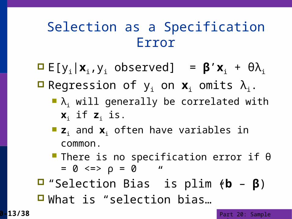
Selection as a Specification Error
E[yi|xi,yi observed] = β’xi + θλi
Regression of yi on xi omits λi. λi will generally be correlated with xi if zi is.
zi and xi often have variables in common. There is no specification error if θ = 0 <=> ρ = 0
“Selection Bias” is plim (b – β) What is “selection bias…”

Part 20: Sample Selection20-14/38
Control Function
Labor Force Participation
d* = + u
What is u? Unmeasured factors that motivate LFP, u = (m,a)
Desired Hours
H* = +
What is ? Unmeasured factors that motivate H*, = (m,c)
z
x
= u + w and u share factors, m.
H* = + u + w
Regression of H* on omits u. is the prediction of u.
Note, the problem goes away if = 0.
x
x
Part 20: Sample Selection20-15/38
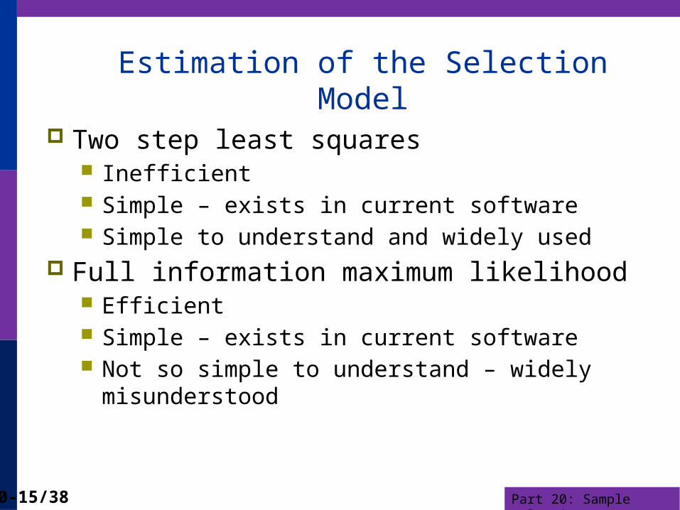
Estimation of the Selection Model Two step least squares
Inefficient Simple – exists in current software Simple to understand and widely used
Full information maximum likelihood Efficient Simple – exists in current software Not so simple to understand – widely misunderstood

Part 20: Sample Selection20-16/38
Estimation
Heckman’s two step procedure (1) Estimate the probit model and compute λi for
each observation using the estimated parameters. (2) a. Linearly regress yi on xi and λi using the
observed data
b. Correct the estimated asymptotic covariance
matrix for the use of the estimated λi. (An
application of Murphy and Topel (1984) – Heckman
was 1979) See text, pp. 876-877.

Part 20: Sample Selection20-17/38
Application – Labor SupplyMROZ labor supply data. Cross section, 753 observationsUse LFP for binary choice, KIDS for count models.LFP = labor force participation, 0 if no, 1 if yes.WHRS = wife's hours worked. 0 if LFP=0KL6 = number of kids less than 6K618 = kids 6 to 18WA = wife's ageWE = wife's educationWW = wife's wage, 0 if LFP=0.RPWG = Wife's reported wage at the time of the interviewHHRS = husband's hoursHA = husband's ageHE = husband's educationHW = husband's wageFAMINC = family incomeMTR = marginal tax rateWMED = wife's mother's educationWFED = wife's father's educationUN = unemployment rate in county of residenceCIT = dummy for urban residence AX = actual years of wife's previous labor market experienceAGE = AgeAGESQ = Age squaredEARNINGS= WW * WHRSLOGE = Log of EARNINGSKIDS = 1 if kids < 18 in the home.
Part 20: Sample Selection20-18/38
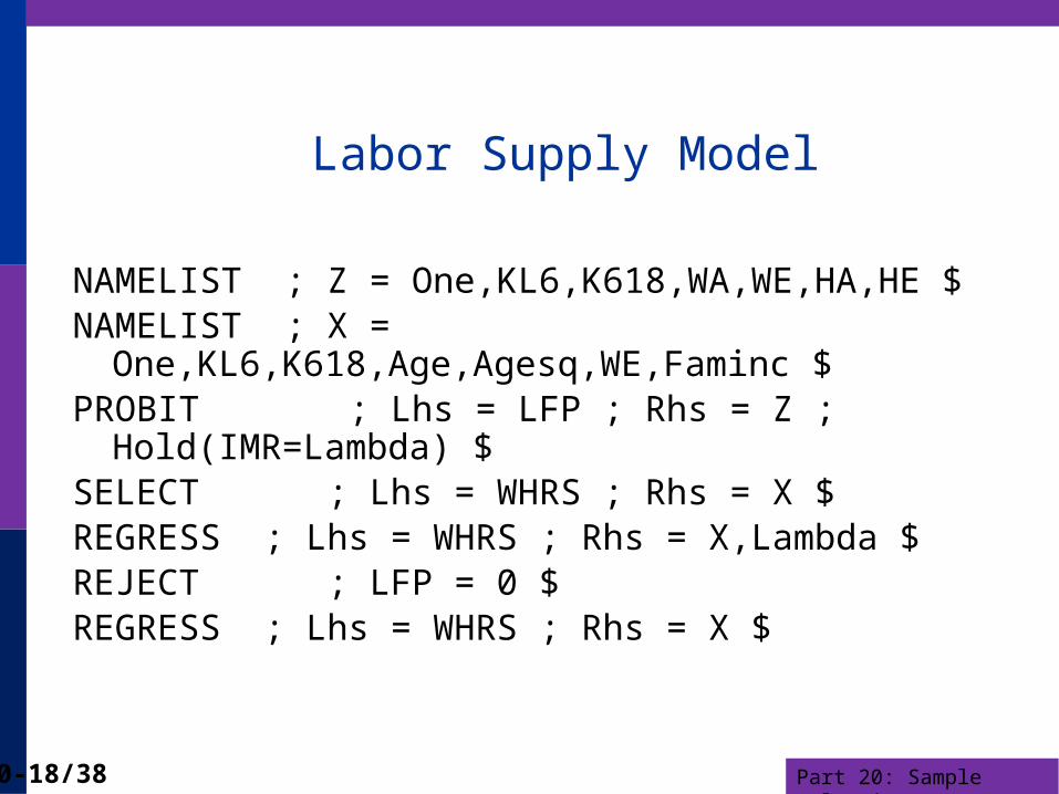
Labor Supply Model
NAMELIST ; Z = One,KL6,K618,WA,WE,HA,HE $NAMELIST ; X = One,KL6,K618,Age,Agesq,WE,Faminc $PROBIT ; Lhs = LFP ; Rhs = Z ; Hold(IMR=Lambda) $SELECT ; Lhs = WHRS ; Rhs = X $REGRESS ; Lhs = WHRS ; Rhs = X,Lambda $ REJECT ; LFP = 0 $REGRESS ; Lhs = WHRS ; Rhs = X $

Part 20: Sample Selection20-19/38
Participation Equation
+---------------------------------------------+| Binomial Probit Model || Dependent variable LFP || Weighting variable None || Number of observations 753 |+---------------------------------------------++---------+--------------+----------------+--------+---------+----------+|Variable | Coefficient | Standard Error |b/St.Er.|P[|Z|>z] | Mean of X|+---------+--------------+----------------+--------+---------+----------+ Index function for probability Constant 1.00264501 .49994379 2.006 .0449 KL6 -.90399802 .11434394 -7.906 .0000 .23771580 K618 -.05452607 .04021041 -1.356 .1751 1.35325365 WA -.02602427 .01332588 -1.953 .0508 42.5378486 WE .16038929 .02773622 5.783 .0000 12.2868526 HA -.01642514 .01329110 -1.236 .2165 45.1208499 HE -.05191039 .02040378 -2.544 .0110 12.4913679

Part 20: Sample Selection20-20/38
Hours Equation+----------------------------------------------------+| Sample Selection Model || Two stage least squares regression || LHS=WHRS Mean = 1302.930 || Standard deviation = 776.2744 || WTS=none Number of observs. = 428 || Model size Parameters = 8 || Degrees of freedom = 420 || Residuals Sum of squares = .2267214E+09 || Standard error of e = 734.7195 || Correlation of disturbance in regression || and Selection Criterion (Rho)........... -.84541 |+----------------------------------------------------++---------+--------------+----------------+--------+---------+----------+|Variable | Coefficient | Standard Error |b/St.Er.|P[|Z|>z] | Mean of X|+---------+--------------+----------------+--------+---------+----------+ Constant 2442.26665 1202.11143 2.032 .0422 KL6 115.109657 282.008565 .408 .6831 .14018692 K618 -101.720762 38.2833942 -2.657 .0079 1.35046729 AGE 14.6359451 53.1916591 .275 .7832 41.9719626 AGESQ -.10078602 .61856252 -.163 .8706 1821.12150 WE -102.203059 39.4096323 -2.593 .0095 12.6588785 FAMINC .01379467 .00345041 3.998 .0001 24130.4229 LAMBDA -793.857053 494.541008 -1.605 .1084 .61466207
Part 20: Sample Selection20-21/38
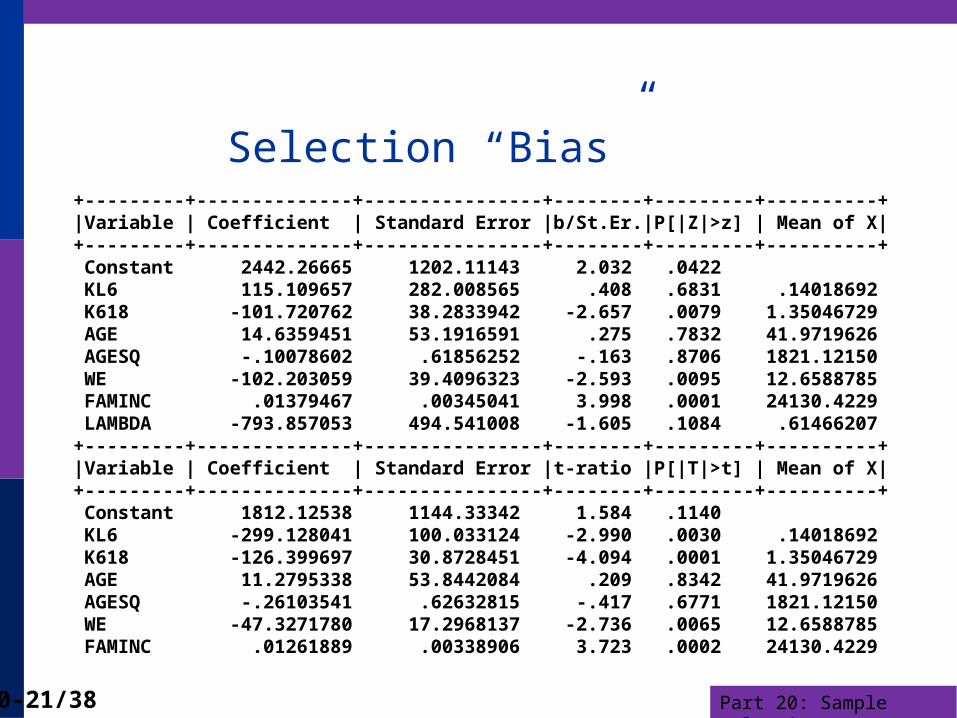
Selection “Bias”+---------+--------------+----------------+--------+---------+----------+|Variable | Coefficient | Standard Error |b/St.Er.|P[|Z|>z] | Mean of X|+---------+--------------+----------------+--------+---------+----------+ Constant 2442.26665 1202.11143 2.032 .0422 KL6 115.109657 282.008565 .408 .6831 .14018692 K618 -101.720762 38.2833942 -2.657 .0079 1.35046729 AGE 14.6359451 53.1916591 .275 .7832 41.9719626 AGESQ -.10078602 .61856252 -.163 .8706 1821.12150 WE -102.203059 39.4096323 -2.593 .0095 12.6588785 FAMINC .01379467 .00345041 3.998 .0001 24130.4229 LAMBDA -793.857053 494.541008 -1.605 .1084 .61466207+---------+--------------+----------------+--------+---------+----------+|Variable | Coefficient | Standard Error |t-ratio |P[|T|>t] | Mean of X|+---------+--------------+----------------+--------+---------+----------+ Constant 1812.12538 1144.33342 1.584 .1140 KL6 -299.128041 100.033124 -2.990 .0030 .14018692 K618 -126.399697 30.8728451 -4.094 .0001 1.35046729 AGE 11.2795338 53.8442084 .209 .8342 41.9719626 AGESQ -.26103541 .62632815 -.417 .6771 1821.12150 WE -47.3271780 17.2968137 -2.736 .0065 12.6588785 FAMINC .01261889 .00338906 3.723 .0002 24130.4229

Part 20: Sample Selection20-22/38
Maximum Likelihood Estimation
z
z
z
21i2 i i
d 1 2
id=0
i i
2
exp ( / ) ( / ) 'logL log
2 1
+ log 1 ( ' )
Reparameterize this: let q '
(1) = 1/
(2) = / (Olsen transformation)
(3) = / 1-
(4) Constrain
x
x
1 -112 1
21 1i i2 2
id 0 d 1 2i i
to be in (-1,1) by using
exp(2 ) 1 = ln atanh ,so =atanh ( )
exp(2 ) 1
log log2 ( y ' )logL log ( q)
log [ ( y ' ) q 1 ]
Part 20: Sample Selection20-23/38
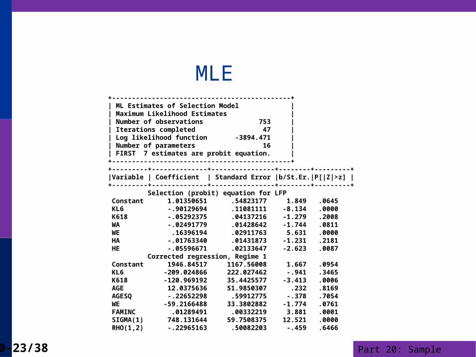
MLE+---------------------------------------------+| ML Estimates of Selection Model || Maximum Likelihood Estimates || Number of observations 753 || Iterations completed 47 || Log likelihood function -3894.471 || Number of parameters 16 || FIRST 7 estimates are probit equation. |+---------------------------------------------++---------+--------------+----------------+--------+---------+|Variable | Coefficient | Standard Error |b/St.Er.|P[|Z|>z] |+---------+--------------+----------------+--------+---------+ Selection (probit) equation for LFP Constant 1.01350651 .54823177 1.849 .0645 KL6 -.90129694 .11081111 -8.134 .0000 K618 -.05292375 .04137216 -1.279 .2008 WA -.02491779 .01428642 -1.744 .0811 WE .16396194 .02911763 5.631 .0000 HA -.01763340 .01431873 -1.231 .2181 HE -.05596671 .02133647 -2.623 .0087 Corrected regression, Regime 1 Constant 1946.84517 1167.56008 1.667 .0954 KL6 -209.024866 222.027462 -.941 .3465 K618 -120.969192 35.4425577 -3.413 .0006 AGE 12.0375636 51.9850307 .232 .8169 AGESQ -.22652298 .59912775 -.378 .7054 WE -59.2166488 33.3802882 -1.774 .0761 FAMINC .01289491 .00332219 3.881 .0001 SIGMA(1) 748.131644 59.7508375 12.521 .0000 RHO(1,2) -.22965163 .50082203 -.459 .6466

Part 20: Sample Selection20-24/38
MLE vs. Two StepTwo Step Constant 2442.26665 1202.11143 2.032 .0422 KL6 115.109657 282.008565 .408 .6831 .14018692 K618 -101.720762 38.2833942 -2.657 .0079 1.35046729 AGE 14.6359451 53.1916591 .275 .7832 41.9719626 AGESQ -.10078602 .61856252 -.163 .8706 1821.12150 WE -102.203059 39.4096323 -2.593 .0095 12.6588785 FAMINC .01379467 .00345041 3.998 .0001 24130.4229 LAMBDA -793.857053 494.541008 -1.605 .1084 .61466207| Standard error of e = 734.7195 || Correlation of disturbance in regression || and Selection Criterion (Rho)........... -.84541 |MLE Constant 1946.84517 1167.56008 1.667 .0954 KL6 -209.024866 222.027462 -.941 .3465 K618 -120.969192 35.4425577 -3.413 .0006 AGE 12.0375636 51.9850307 .232 .8169 AGESQ -.22652298 .59912775 -.378 .7054 WE -59.2166488 33.3802882 -1.774 .0761 FAMINC .01289491 .00332219 3.881 .0001 SIGMA(1) 748.131644 59.7508375 12.521 .0000 RHO(1,2) -.22965163 .50082203 -.459 .6466

Part 20: Sample Selection20-25/38
How to Handle Selectivity The ‘Mills Ratio’ approach – just add a ‘lambda’
to whatever model is being estimated? The Heckman model applies to a probit model with a
linear regression. The conditional mean in a nonlinear model is not
something “+lambda” The model can sometimes be built up from first
principles
Part 20: Sample Selection20-26/38
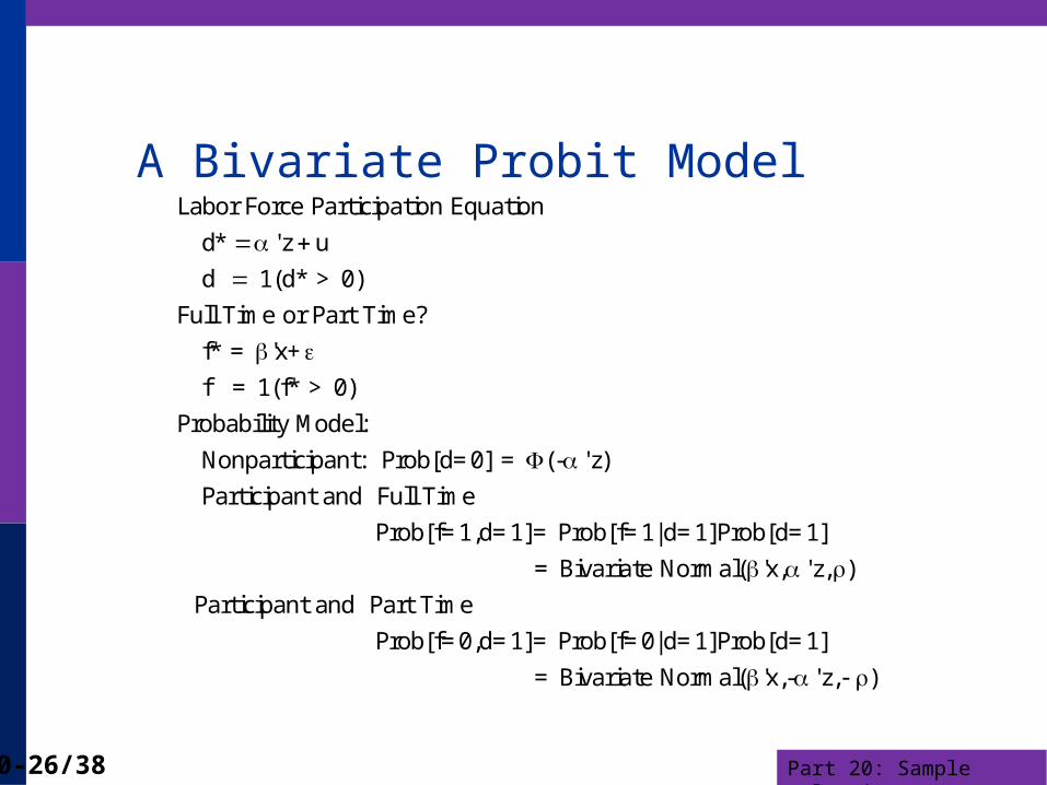
A Bivariate Probit ModelLabor Force Participation Equation
d* 'z u
d 1(d* > 0)
Full Time or Part Time?
f* = 'x+
f = 1(f* > 0)
Probability Model:
Nonparticipant: Prob[d=0] = (- 'z)
Participant and Full Ti
me
Prob[f=1,d=1]= Prob[f=1|d=1]Prob[d=1]
= Bivariate Normal( 'x, 'z, )
Participant and Part Time
Pro
b[f=0,d=1]= Prob[f=0|d=1]Prob[d=1]
= Bivariate Normal( 'x,- 'z, )

Part 20: Sample Selection20-27/38
FT/PT Selection Model+---------------------------------------------+| FIML Estimates of Bivariate Probit Model || Dependent variable FULLFP || Weighting variable None || Number of observations 753 || Log likelihood function -723.9798 || Number of parameters 16 || Selection model based on LFP |+---------------------------------------------++---------+--------------+----------------+--------+---------+----------+|Variable | Coefficient | Standard Error |b/St.Er.|P[|Z|>z] | Mean of X|+---------+--------------+----------------+--------+---------+----------+ Index equation for FULLTIME Constant .94532822 1.61674948 .585 .5587 WW -.02764944 .01941006 -1.424 .1543 4.17768154 KL6 .04098432 .26250878 .156 .8759 .14018692 K618 -.13640024 .05930081 -2.300 .0214 1.35046729 AGE .03543435 .07530788 .471 .6380 41.9719626 AGESQ -.00043848 .00088406 -.496 .6199 1821.12150 WE -.08622974 .02808185 -3.071 .0021 12.6588785 FAMINC .210971D-04 .503746D-05 4.188 .0000 24130.4229 Index equation for LFP Constant .98337341 .50679582 1.940 .0523 KL6 -.88485756 .11251971 -7.864 .0000 .23771580 K618 -.04101187 .04020437 -1.020 .3077 1.35325365 WA -.02462108 .01308154 -1.882 .0598 42.5378486 WE .16636047 .02738447 6.075 .0000 12.2868526 HA -.01652335 .01287662 -1.283 .1994 45.1208499 HE -.06276470 .01912877 -3.281 .0010 12.4913679 Disturbance correlation RHO(1,2) -.84102682 .25122229 -3.348 .0008
Full Time = Hours > 1000
Part 20: Sample Selection20-28/38
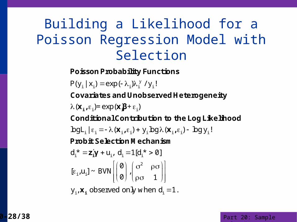
Building a Likelihood for a Poisson Regression Model with Selection
yi i i i i
i i
i i i i i i i i
P(y | x ) exp( ) / y !
( )=exp( + )
logL | ( ) y log ( ) logy !
i i
Poisson Probability Functions
Covariates and Unobserved Heterogeneity
x , xβ
Conditional Contribution to the Log Likelihood
x , x ,
Pr
i i i i
2
i i
i i
d* u , d 1[d* 0]
0[ ,u] ~BVN ,
0 1
y , observed only when d 1.
i
i
obit Selection Mechanism
z γ
x
Part 20: Sample Selection20-29/38
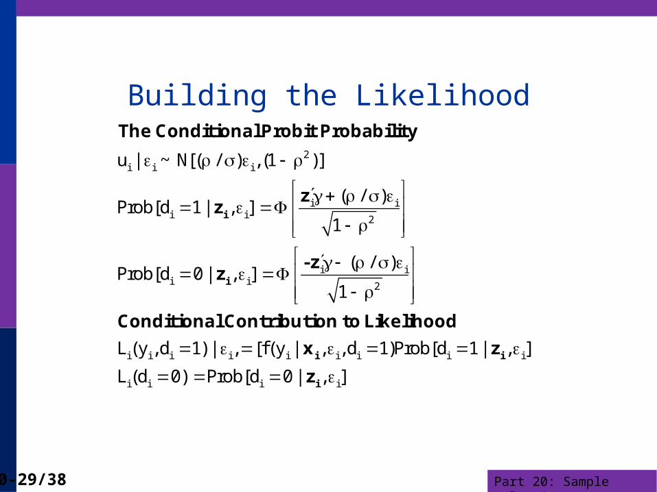
Building the Likelihood
2i i i
i ii i 2
i ii i 2
i i i i
u | ~N[( / ) ,(1 )]
( / )Prob[d 1| , ]
1
( / )Prob[d 0| , ]
1
L (y ,d 1) | , [f(y
i
i
The Conditional Probit Probability
zz
-zz
Conditional Contribution to Likelihood
i i i i i
i i i i
| , ,d 1)Prob[d 1| , ]
L (d 0) Prob[d 0| , ]
i i
i
x z
z

Part 20: Sample Selection20-30/38
Conditional Likelihood
i i i i i i i i
i i i i i
i i i i i i i
i i
f(y ,d 1| ) [f(y | ,d 1)]Prob[d 1| ]
f(y ,d 0| ) Prob[d 0| ]
1f(y ,d 1) [f(y | ,d 1)]Prob[d 1| ] d
f(y ,d 0) Prob
Conditional Density (not the log)
Unconditional Densities
i i
i i i
1[d 0| ] d
logL logf(y ,d)
Log Likelihoods
Part 20: Sample Selection20-31/38
Poisson Model with Selection Strategy:
Hermite quadrature or maximum simulated likelihood. Not by throwing a ‘lambda’ into the unconditional
likelihood Could this be done without joint normality?
How robust is the model? Is there any other approach available? Not easily. The subject of ongoing research

Part 20: Sample Selection20-32/38
Nonnormality Issue How robust is the Heckman model to
nonnormality of the unobserved effects? Are there other techniques
Parametric: Copula methods Semiparametric: Klein/Spady and Series methods
Other forms of the selection equation – e.g., multinomial logit
Other forms of the primary model: e.g., as above.

Part 20: Sample Selection20-33/38
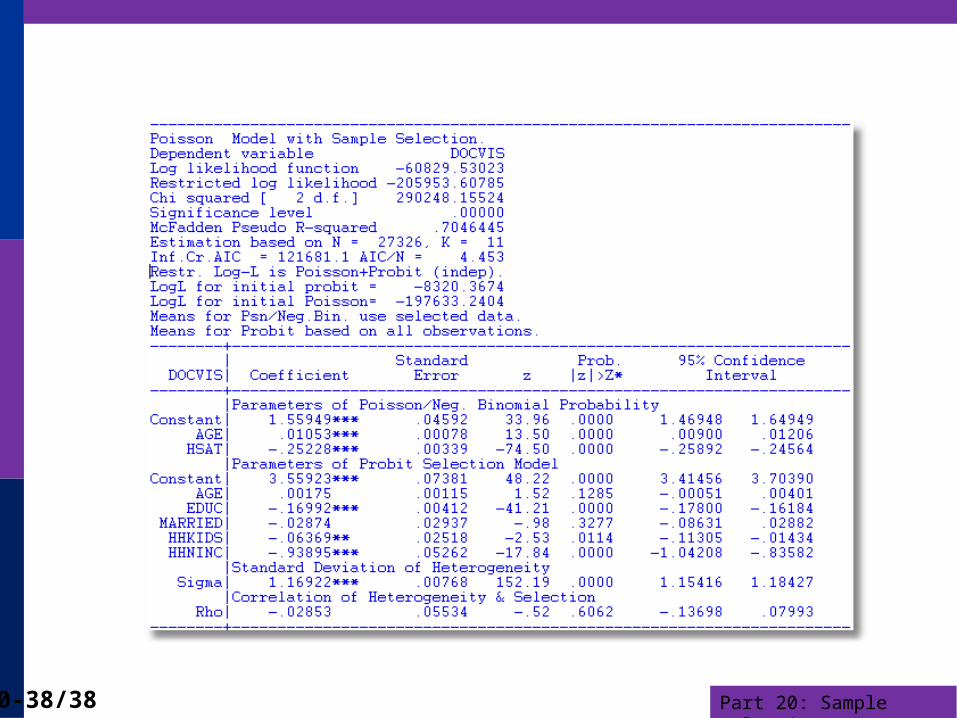
Application: Health Care UsageGerman Health Care Usage Data, 7,293 Individuals, Varying Numbers of PeriodsThis is an unbalanced panel with 7,293 individuals. There are altogether 27,326 observations. The number of observations ranges from 1 to 7. (Frequencies are: 1=1525, 2=2158, 3=825, 4=926, 5=1051, 6=1000, 7=987). (Downloaded from the JAE Archive)Variables in the file are DOCTOR = 1(Number of doctor visits > 0) HOSPITAL = 1(Number of hospital visits > 0) HSAT = health satisfaction, coded 0 (low) - 10 (high) DOCVIS = number of doctor visits in last three months HOSPVIS = number of hospital visits in last calendar year PUBLIC = insured in public health insurance = 1; otherwise = 0 ADDON = insured by add-on insurance = 1; otherswise = 0 HHNINC = household nominal monthly net income in German marks / 10000. (4 observations with income=0 were dropped) HHKIDS = children under age 16 in the household = 1; otherwise = 0 EDUC = years of schooling AGE = age in years MARRIED = marital status

Part 20: Sample Selection20-34/38

Part 20: Sample Selection20-35/38

Part 20: Sample Selection20-36/38

Part 20: Sample Selection20-37/38
Part 20: Sample Selection20-38/38

Part 20: Sample Selection20-39/38