Part A: Integration

Alison Etheridge

1 Introduction

In Mods you learned how to integrate step functions and continuous functions on closed boundedintervals. We begin by recalling some of that theory.

Definition 1.1 (Step functions and their integrals). A function φ defined on the interval I (withendpoints a, b) is a step function if there is a partition (ai)ki=0 of the interval (that is a = a0 < a1 <a2 < . . . < ak = b) so that φ is constant on each interval (aj−1, aj), j ≤ k.

If φ(x) = ci for x ∈ (ai−1, ai), then∫Iφ ≡

∫Iφ(x)dx =

k∑i=1

ci(ai − ai−1).

Write Lstep[a, b] for the space of step functions on [a, b].

Definition 1.2 (Lower and Upper Sums). For a real-valued function on [a, b] define∫ b

af = sup

∫ b

aφ : φ ∈ Lstep[a, b], φ ≤ f

,

∫ b

af = inf

∫ b

aφ : φ ∈ Lstep[a, b], φ ≥ f

The fundamental result that you proved was the following.

Theorem 1.3 (Integrating continuous functions over closed bounded intervals). For a continuousfunction f on the closed bounded interval [a, b]∫ b

af =

∫ b

af. (1)

The quantity in equation (1) is then defined to be the integral of f over [a, b]. We write C[a, b] forcontinuous functions on [a, b].

Later in the course you considered sequences of continuous functions:

Theorem 1.4 (Exchanging integrals and limits under uniform convergence). Let fnn≥1 be a sequenceof functions in C[a, b] for which fn → f uniformly (and so in particular f ∈ C[a, b]) then∫ b

afn →

∫ b

af as n→∞.

1

You then exploited this to interchange summation and integration for power series: Suppose that thepower series f(t) =

∑∞k=0 akt

k has radius of convergence R. Write fn(t) =∑n

k=0 aktk. Since for

|x| < R, fn(t)→ f(t) uniformly on [0, x] you deduced that∫ x

0f(t)dt = lim

n→∞

∫ x

0fn(t)dt

= limn→∞

n∑k=0

akxk+1

k + 1

=∞∑k=0

akxk+1

k + 1,

and this proved to be a powerful tool in establishing deep properties of exponential and trigonometricfunctions.

Originally integration was introduced as the inverse of differentiation. The goal of Newton (1642–1727) and Leibniz (1646 – 1716) was to solve the problem of primitives:

Find the functions F (x) which have derivative a given function f(x).

At that time the notion of function was not really well defined, but usually it meant associating aquantity y to a variable x through an equation involving arithmetic operations (addition, subtraction,multiplication, division, taking roots), trigonometric operations (sin, cos, tan and their inverses) andlogarithms and exponentials.

With the geometric understanding of integration as area under a curve came the generalisation ofthis idea of function, but still continuous functions were viewed as the ‘real’ functions and the notion ofintegration from Mods sufficed. The version of the Fundamental Theorem of Calculus that you provedin Mods showed that for continuous functions f on closed bounded intervals, the problem of primitiveswas solved by the indefinite integral of f . But then along came Fourier (1768–1830). He showed thattrigonometric series which can be used to represent continuous functions on bounded intervals can alsobe used to represent discontinuous ones. In particular, the function

f(x) =

0 0 ≤ x ≤ π,1 π < x ≤ 2π,

can be represented by a convergent trigonometric series. The notion of function had to be extendedand with it the notion of integral.

For a finite number of discontinuities, one can piece together the portions on which the functionis continuous and your methods easily extend - and in fact you can even go a bit further providedthe points of discontinuity are ‘exceptional’ in a sense that we’ll make precise later. But worse was tocome. Dirichlet (1805–1859) came across the following function which now takes his name:

Definition 1.5 (Dirichlet function). The function

χ(x) =

1 if x ∈ Q,0 if x /∈ Q, (2)

is known as the Dirichlet function.

In fact Dirichlet obtained χ as a limit:

χ(x) = limm→∞

limn→∞

(cos(m!πx))2n .

2

The Dirichlet function is nowhere continuous and yet Dirichlet constructed it as a double pointwiselimit of a sequence of continuous functions.

Evidently our theory of integration from Mods really cannot handle the Dirichlet function. Anystep function φ on [0, 1] satsifying φ ≤ χ also satisfies φ ≤ 0 on [0, 1] and the constant step function0 on [0, 1] satisfies 0 ≤ χ and so

∫ 10 χ(x)dx = 0. Likewise, the constant function step function 1 on

[0, 1] satisfies 1 ≥ χ and any step function φ on [0, 1] satisfying χ ≤ φ also satisfies φ ≥ 1 on [0, 1], so∫ 10 χ(x)dx = 1. Thus

0 =∫ 1

0χ(x)dx <

∫ 1

0χ(x)dx = 1.

Of course there are many other less perverse ways than Dirichlet’s to obtain the Dirichlet function asa pointwise limit of functions that are integrable in the sense of Mods.

Example 1.6. Let rnn≥1 be an enumeration of the rationals in [0, 1]. For each k ∈ N definefk : [0, 1]→ R by

fk(x) =

1 x = rn, 1 ≤ n ≤ k,0 otherwise.

Then∫fk(x)dx = 0 for each k, but

∫limk→∞ fk(x)dx is not (yet) defined.

The Lebesgue integral, introduced by Lebesgue in a very short paper of 1901 but fully explained ina beautiful set of lecture notes published in 1904 (from a course delivered in 1902-3) is an extension ofthe integral that you developed in Mods that behaves well under passage to the limit.

So when will it be the case that fn → f implies∫fn →

∫f in our new theory? The next example

shows that the answer should certainly be not always.

Example 1.7. Define fk : [0, 1]→ R by

fk(x) =k(1− kx) 0 ≤ x ≤ 1/k,

0 otherwise.

Each fk is continuous and fk(x)→ 0 as k →∞ for all x ∈ (0, 1]. So fk → f ≡ 0. But∫ 1

0 fk(x)dx = 1/2for all k. So

0 =∫ 1

0limk→∞

fk(x)dx < limk→∞

∫ 1

0fk(x)dx =

12.

The difficulty from the point of view of the integration theory of Mods is that the convergence isnot uniform. It will turn out that we’ll get convergence theorems for our new integral under otherconditions. For example, suppose that we restrict ourselves to functions with |fk(x)| ≤M for all k andall x ∈ [0, 1]. A theorem with this hypothesis is called a bounded convergence theorem. Or, becausewe don’t want to restrict ourselves to bounded functions on bounded intervals, we could try takinga monotone sequence fk ↑ f (by which we mean that fk ≤ fk+1 for all k and fk → f) or fk ↓ f .A theorem with this hypothesis is called a monotone convergence theorem. Example 1.6 shows thatneither of these conditions is enough to rescue the integral of Mods, but they will help us out here. Thefunctions of Example 1.7 don’t satisfy either of our hypotheses and we agreed that for them we wouldnot expect a convergence theorem. It was natural that the integral of the limit was strictly less thanthe limit of the integrals. We’ll see that for positive functions an inequality a bit like this always holds.The limit of the integrals might not exist and so we replace it with a new concept that we’ll definelater called the lim inf. When the limit does exist then it is equal to the lim inf. Probably the most

3

important result of our theory, Fatou’s Lemma, will tell us that for positive functions fk converging tof ∫

limk→∞

fk(x)dx ≤ lim infk→∞

∫fk(x)dx.

So what should the integral of the Dirichlet function of Definition 1.5 over [0, 1] be?The Dirichlet function is just the indicator function of the rationals. For an interval I we define

the integral of its indicator function over [0, 1] to be the length of I ∩ [0, 1]. Similarly for a set S whichis a finite union of disjoint intervals, the integral over [0, 1] of the indicator function of S is the totallength of the intervals making up S ∩ [0, 1]. For an interval [a, b] we’ll write m([a, b]) = b − a for itslength. It would make sense then for the integral of the Dirichlet function over [0, 1] to be the ‘length’of the set Q ∩ [0, 1], m(Q ∩ [0, 1]). So now we have to work out how to assign a length to this set.

For two sets A ⊆ B our intuition says that the length of A should be less than or equal to that ofB, that is m(A) ≤ m(B). Now, given ε > 0, let rnn≥1 be an enumeration of the rationals in [0, 1]and let

In = (rn −ε

2n+1, rn +

ε

2n+1),

then Q ∩ [0, 1] ⊆⋃∞n=1 In and (again using a bit of intuition) the total length of the right hand side is

less than or equal to∑∞

n=1ε

2n = ε. Since ε was arbitrary we conclude that in a reasonable world we’dbetter take the length of Q ∩ [0, 1] to be zero. We’ll make that more precise later, but then with thisnotion of length, ∫ 1

0χ(x)dx = 0

and our problem with the functions fkk≥1 of Example 1.6 goes away,

0 =∫ 1

0χ(x)dx =

∫ 1

0limk→∞

fk(x)dx = limk→∞

∫ 1

0fk(x)dx.

What we’ve done in this example, instead of trying to approximate χ by step functions based onintervals, is we’ve asked what is the ‘length’ or (as we’ll usually say) measure of the set where χ isequal to one. Lebesgue’s key idea was to extend this.

To approximate a function by stepfunctions as you did in Mods, you divide

the domain of the function.To approximate a function by simple

functions, as we’ll do here, we divide therange of the function.

The simple function in the right hand picture is defined to be

4∑k=1

yk−11Sk(x)

where Sk = x ∈ R : yk−1 ≤ f(x) < yk and 1S is the indicator function of the set S. Of course in thispicture the simple function is a step function. But in general it won’t be, as we saw in our Dirichletfunction example where it was the indicator function of Q∩ [0, 1]. (See problem sheet 1 for an exampleof a continuous function for which Lebesgue’s recipe does not always give a step function.)

Exercise 1.8. As another example try approximating sin 1x on (0, 1] by simple functions.

Here then is Lebesgue’s recipe for integrating a bounded function over an interval [a, b]:

4

1. Subdivide the y-axis by a series of points

minx∈[a,b]

f(x) ≥ y0 < y1 < · · · < yn > maxx∈[a,b]

f(x).

2. Form the sumn∑k=1

yk−1 ×measure (x ∈ [a,b] : yk−1 ≤ f(x) < yk) .

3. Let the number of points yn go to infinity in such a way that max(yk − yk−1)→ 0.

The limit of the sequence of sums in 2 is∫ ba f(x)dx.

In fact we’ll see that for bounded functions on [a, b]∫ b

af(x)dx = inf

∫ b

aψ(x)dx : ψ simple , ψ ≥ f = sup

∫ b

aφ(x)dx : φ simple , φ ≤ f,

so when a function is integrable in the sense of Mods we’ll get exactly the same answer as before. Butbecause

step functions ( simple functions

we can define the integral for a wider class of functions this way. Moreover, our recipe just needs us tobe able to assign a value to

measure (x : yk−1 ≤ f(x) < yk)

so now we’re not restricted to integrating functions f : R → R over intervals. We can integratefunctions f : Ω → R over any subset of Ω provided we have a suitable notion of size of sets where ftakes particular values. In particular, Ω could be a probability space or Z or N or a sphere or a torusor . . ..

To see the power (and limitations) of the theory though we need to know which sets we can measure.So our first task is going to be to develop a theory of measure.

BUT FIRST:Please remember that you can still integrate everything that you already know how to integrate.

Lebesgue integration extends the theory of Mods so that you can integrate more functions than before.In particular, you can still integrate continous functions over closed bounded intervals and techn-

niques that you justified in Mods like integration by parts and substitution can still be used for thosefunctions. Thus you may freely use the following results from your Analysis III notes:

Theorem 1.9 (Integration by parts). If u, v are differentiable on [a, b] and u′, v′ are in C[a, b] then∫ b

a(u′v) +

∫ b

a(uv′) = u(b)v(b)− u(a)v(a).

Theorem 1.10 (Substitution). Suppose that g ∈ C([c, d]) is strictly monotone increasing and con-tinuously differentiable (so g′ ∈ C[c, d] and g′ > 0) and suppose that g(c) = a, g(d) = b. Then forf ∈ C[a, b] ∫ d

cf (g(x)) g′(x)dx =

∫ b

af(x)dx.

5

2 Lebesgue measurable sets in R

In this section we concentrate on the problem that motivated Lebesgue. Here’s the problem that heproposes:

We wish to attach a non-negative real number which we shall call the measure m(E) toeach bounded subset of R in such a way that the following conditions are satisfied:

1. If E′ is a translation of E then m(E′) = m(E).

2. If Eii is a finite or countably infinite collection of sets with Ei ∩ Ej = ∅ wheneveri 6= j then

m

(⋃i

Ei

)=∑i

m(Ei).

3. m((0, 1)) = 1.

Let’s pause to think about 2. It seems reasonable that if I split a set into two disjoint pieces E = E1∪E2

with E1 ∩E2 = ∅ say, then m(E) = m(E1) +m(E2). But we’re asking for something a bit stronger. IfEi∞i=1 is a countably infinite family of sets with Ei ∩ Ej = ∅ for i 6= j, then writing

E =∞⋃i=1

Ei

and

Bn = E\n⋃i=1

Ei

then if we are going to have any hope of developing a theory that behaves well under passage tothe limit, it is reasonable to ask for a kind of ‘continuity’ property, namely that if m(E) < ∞ thenm(Bn)→ 0 as n→∞. If we assume that 2 holds for finite collections of sets then this becomes

m(Bn) = m(E)−m

(n⋃i=1

Ei

)= m(E)−

n∑i=1

m(Ei)→ 0 as n→∞.

That is

m(E) = limn→∞

m(n⋃i=1

Ei) = limn→∞

n∑i=1

m(Ei) =∞∑i=1

m(Ei),

which is what 2 says for countable disjoint unions.A consequence of Lebesgue’s three conditions is (see Problem Sheet 1) that for any interval I = [a, b]

(or (a, b], [a, b), (a, b)), the measure m(I) = b− a. So Lebesgue measure is required to be an extensionof our notion of length of an interval. It turns out (but it is beyond our scope in this course) that ifwe were to weaken 2 by only requiring this property for finite collections, then one can define a notionof length for all subsets of R. But we are interested in countable operations (it was interchange oflimits and integration that motivated us) so we need this stronger version and then one can constructsets to which it is not possible to assign a measure. This was first achieved by Vitali and we’ll see (avariant of) his famous set in Example 2.12. On the other hand it turns out that one has to work hardto construct a non-measurable set and so we shall not be greatly inconvenienced by their existence.

Lebesgue’s approach to constructing his measure owes a lot to the upper and lower sums of theintegration theory from Mods. The key idea is the one that we used to suggest that the ‘length’ ofQ ∩ [0, 1] (that arose in integrating the Dirichlet function over [0, 1]) should be zero.

6

Recall that Lebesgue’s conditions already tell us that the measure of an interval with endpoints aand b (with a < b say) is b − a. (We also allow intervals to be empty in which case they have lengthzero.)

Definition 2.1 (Outer measure). For a set E ⊆ R, the outer measure of E is

m∗(E) = inf

∞∑n=1

m(In) : E ⊆∞⋃n=1

In, In intervals

.

What we showed in §1 was that m∗ (Q ∩ [0, 1]) = 0.

Definition 2.2 (Null sets). A set E ⊆ R is null (with respect to Lebesgue measure) if m∗(E) = 0.

Lemma 2.3 (Some properties of null sets). 1. Any subset of a null set is null.

2. A countable union of null sets is null.

WARNING: NOT ALL NULL SETS ARE COUNTABLE.

The proof of Lemma 2.3 and an example of an uncountable null set are both on Problem Sheet 1.

Lemma 2.4 (Some properties of outer measure). 1. If E′ is a translation of E then m∗(E′) =m∗(E).

2. If Eii is a finite or countably infinite collection of sets then

m∗(⋃i

Ei) ≤∑i

m∗(Ei).

3. m∗([a, b]) = b− a.

The difficulty is 2. It tells us that m∗ is countably subadditive, but we cannot deduce that it is countablyadditive which was Lebesgue’s condition 2.

Exercise 2.5. Prove 2. If you get stuck look in, for example, Capinski & Kopp.

The outer measure is really playing the role of the upper sum in our old definition of the integral if wetry to define the integral of the indicator function of a set E. To define measurable sets we need ananalogue of the lower sum. Lebesgue provided this with the inner measure.

Definition 2.6 (Inner measure). For a subset E of the interval [a, b], the inner measure of E is givenby

m∗(E) = m∗ ([a, b])−m∗ ([a, b]\E)= b− a−m∗ ([a, b]\E) .

Definition 2.7 (Lebesgue measurable sets). A subset E of R is Lebesgue measurable if for each boundedinterval I

m∗(E ∩ I) +m∗(Ec ∩ I) = m∗(I).

Its Lebesgue measure is then equal to its outer measure. When a set E is Lebesgue measurable wedenote its Lebesgue measure by m(E).

7

Notice in particular that all bounded intervals are Lebesgue measurable. We can deduce from thisdefinition that a set E is Lebesgue measurable if and only if, for every finite interval I, the inner andouter measures of the set E ∩ I agree.

Theorem 2.8. The outer measure m∗ restricted to the Lebesgue measurable sets satisfies Lebesgue’sconditions 1, 2 and 3.

This Theorem tells us that by restricting to the Lebesgue measurable sets we have overcome thedifficulties of outer measure and recovered countable additivity. This is only going to be a good theoryif the class of Lebesgue measurable sets is sufficiently large. So which sets are Lebesgue measurable?

Theorem 2.9. The class of Lebesgue measurable sets, denoted MLeb, has the following properties:

1. R ∈MLeb.

2. If E ∈MLeb then Ec ∈MLeb.

3. If En ∈MLeb for all n ∈ N then⋃∞n=1En ∈MLeb.

This Theorem says thatMLeb forms what is called a σ-algebra. It is closed under finite or countable setoperations. In particular you can check, using de Morgan’s laws, that the intersection of a countablecollection of Lebesgue measurable sets is also Lebesgue measurable.

Proofs of Theorems 2.8 and 2.9 can be found, for example, in Temple (1971), Chapter 7. Thereis also a proof in Capinski & Kopp, but they take a different definition of Lebesgue measurable sets.They assume what is known as the Caratheodory condition, that

m∗(E ∩A) +m∗(Ec ∩A) = m∗(A)

for all A ⊆ R and not just for bounded intervals. Their definition is equivalent to ours, but that is nota very easy thing to show.

As we already remarked, all intervals are Lebesgue measurable and so any set obtained by takingfinite or countable unions or intersections of intervals is Lebesgue measurable. In particular,

Lemma 2.10. All open sets E ⊆ R are Lebesgue measurable.

The class of Lebesgue measurable sets is beginning to look rather big. It is actually slightly larger stillbecause all null sets are Lebesgue measurable (and have Lebesgue measure zero). In fact the Lebesguemeasurable sets are precisely those that can be obtained from intervals and null sets by a finite orcountable sequence of set operations. There are a lot of those sets.

Definition 2.11. The collection of sets that can be obtained by a finite or countable sequence of setoperations from the intervals of R is called the σ-algebra generated by the intervals, or the Borel σ-algebra on R. Supplementing these by taking set operations with sets E with m∗(E) = 0 is known astaking the completion with respect to the (Lebesgue) outer measure and yields the Lebesgue measurablesets.

The next (non-examinable) example illustrates how hard one has to work to construct a non-measurableset. It is a variant of an example due to Vitali. It is convenient to work with the unit circle S1. Thedefinition of measurable set translates in an obvious way since S1 can be thought of as [0, 2π).

Example 2.12 (A non-measurable set). Let

S1 = eiθ : θ ∈ R.

8

Define an equivalence relation on S1 by writing

z ∼ w if ∃α, β ∈ R s.t. z = eiα, w = eiβ, and α− β ∈ Q.

Let A be a set obtained by choosing exactly one representative from each equivalence class. Define

Aq = eiq ·A = eiqz : z ∈ A.

Then Aqq∈Q is a collection of pairwise disjoint sets, each obtained from A by rotation and S1 =⋃q∈QAq.

Suppose that A is measurable, then so is Aq and m(Aq) = m(A) for all q ∈ Q. Then by countableadditivity,

2π = m(S1) =∑q∈Q

m(Aq) =

0 if m(A) = 0∞ if m(A) > 0,

which yields a contradiction.Thus we cannot assign a measure to A.

It turns out that to construct a non-measurable set one has to invoke the ‘axiom of choice’ which iswhat allowed us to choose exactly one representative from each of the uncountably infinite number ofequivalence classes.

In higher dimensions things are even worse. In three dimensions one can cut a solid ball into afinite number of non-overlapping sets which can then be reasssembled to yield two identical copies ofthe original ball. Do a web search on Banach-Tarski paradox to find out more.

3 Other measure spaces

In §2 we saw that we could define a notion of ‘length’ or ‘measure’ for a wide class of subsets of Rcalled the Lebesgue measurable sets. A fancy way to say this is to say that (R,MLeb,m) is a measurespace.

Definition 3.1 (Measure space). We say that (Ω,F , µ) is a measure space if Ω is an abstractly givenset, F is a collection of subsets of Ω which includes ∅ and is closed under complements and finite orcountable unions (recall that this says that F is a σ-algebra) and µ : F → [0,∞] is a countably additiveset function; that is if Enn∈N is a countable collection of sets from F with Ei ∩ Ej = ∅ wheneveri 6= j then

µ

( ∞⋃n=1

En

)=∞∑n=1

µ(En).

There are lots of measure spaces out there, several of which you are already familiar with.

Example 3.2 (Discrete measure theory). Let Ω be a countable set and F the power set of Ω (that isthe collection of all subsets of Ω). A mass function is any function µ : Ω→ [0,∞]. We can then definea measure on Ω by µ(x) = µ(x) and extend to arbitrary subsets of Ω using Property 2.

Equally given a measure on Ω we can define a mass function.In particular,

1. If∑

x∈Ω µ(x) =∑

x∈Ω µ(x) = 1 then µ is a probability measure and µ is the correspondingprobability mass function. For A ⊆ Ω,

µ(A) =∑x∈A

µ(x).

9

The null sets correspond in the terminology of Mods probability to events that have probabilityzero.

2. If Ω = N and µ(k) = 1,∀k ∈ N then we get counting measure. For A ⊆ N,

µ(A) = ]n : n ∈ A.

In this case the only null set is the empty set.

These discrete measure spaces provide a ‘toy’ version of the general theory where each of the resultswe prove for general measure spaces reduces to some straightforward fact about convergence of series.This is all we need to do (for example) discrete probability and so that topic is generally introducedwithout discussing measure theory. But for more general probability and most of analysis (both pureand applied) this is not enough.

Example 3.3. Consider the problem from ‘continuous’ probability of picking a point uniformly from[0, 1]. We face making sense of the ‘probability’ that a given number is chosen or that the numberchosen falls within a particular set. Write U for the (random) point picked. Evidently P[U = x] = 0if all points are equally likely, for otherwise

∑x∈[0,1] P[U = x] =∞. This means that we won’t be able

to distinguish the probabilities of two sets that differ by just one point, or indeed that differ by a finitenumber of points. On the other hand we’d expect to be able to define for an interval I = [a, b] ⊆ [0, 1]

P[U ∈ I] = b− a.

The Lebesgue measurable subsets of [0, 1] are precisely those to which we can assign P[U ∈ A] in aconsistent way.

The measure that we defined on the Lebesgue measurable subsets of R was certainly not the onlymeasure on (R,MLeb). The form that it took was forced upon us by our insistence that m([a, b]) = b−a.

Example 3.4. 1. Define

µ([a, b]) =1√2π

∫ b

ae−x

2/2dx.

Then µ extends to a measure on all the Lebesgue measurable subsets of R. This measure is ofcentral importance in statistics.

2. For [a, b] ⊆ [0,∞) define

µt([a, b]) =∫ b

ae−txdx.

Then for each t > 0, µt extends to a measure on all the Lebesgue measurable subsets of [0,∞).This family of measures is very important in the study of differential equations.

These examples are all of either discrete measures or measures which are absolutely continuous withrespect to Lebesgue measure. We’ll see the origin of that term in §7. But of course one can havemixtures of the two (see Problem Sheet 2 for an example) and in fact in §7 we’ll see that there aremore exotic measures still.

Although mostly we’ll concentrate on Lebesgue measure, always keep in mind that our theory ismuch more general.

10

4 Measurable functions

We now turn our attention to the objects at the heart of integration theory: the measurable functions.Last term in the Analysis course you saw that a function f : X → Y (where X and Y are subsets

of Euclidean space) is continuous if and only if

A open in Y =⇒ f−1(A) open in X.

If you are studying topology then you’ll know that this definition applies more generally. For thedefinition of measurable functions we’ll replace ‘open’ by ‘measurable’. The advantage of measurablefunctions over continuous functions is that they are much more ‘stable’. In particular, they behavewell under limits: the pointwise limit of a sequence of measurable functions is measurable - and this‘closure’ of the space of measurable functions is at the heart of the convergence theorems.

Definition 4.1 (Measurable function). Let (Ω,F , µ) and (Λ,G, ν) be measure spaces. A functionf : Ω→ Λ is measurable (with respect to F , G) if and only if

G ∈ G =⇒ f−1(G) ∈ F .

For concreteness, mostly we’re going to work in the special setting of Lebesgue measurable functionson R. But the arguments that we use will be insensitive to replacing the Lebesgue measurable sets,MLeb, by F of Definition 4.1.

Definition 4.2 (Lebesgue measurable function). A function f : R→ R is Lebesgue measurable if andonly if for every interval I ⊆ R, f−1(I) = x ∈ R : f(x) ∈ I is a Lebesgue measurable set.

Similarly, if E is a measurable subset of R, then f : E → R is Lebesgue measurable if for eachinterval I, f−1(I) is Lebesgue measurable.

In what follows, if we say that f : R → R is measurable, without further qualification, then we meanLebesgue measurable.

The definition is equivalent to requiring that for all Borel sets A, f−1(A) is Lebesgue measurable.The point is that it is enough to check just for intervals and indeed we don’t need to check it for allintervals I. It is convenient to know the following result.

Theorem 4.3. Let E be a measurable subset of R and f : E → R be a function. The following areequivalent:

1. f is measurable.

2. For all a, f−1((a,∞)) is measurable.

3. For all a, f−1([a,∞)) is measurable.

4. For all a, f−1(−∞, a)) is measurable.

5. For all a, f−1(−∞, a]) is measurable.

Proof. Let’s just prove one of these. Obviously (1) implies all the others. We prove here that(2) =⇒ (1).

We must show that for any interval I, f−1(I) ∈MLeb. We already have that f−1((a,∞)) ∈MLeb.Now suppose that I = (−∞, a].

f−1((−∞, a]) = f−1(R\(a,∞)) = E\f−1((a,∞)) ∈MLeb

11

since measurable sets are closed under taking complements.Now note that

f−1((−∞, b)) = f−1

( ∞⋃n=1

(−∞, b− 1n

]

)

=∞⋃n=1

f−1((−∞, b− 1n

]) ∈MLeb

since countable unions of measurable sets are measurable. Taking complements we also have f−1(([b,∞)) ∈MLeb.

Now let I = (a, b).

f−1((a, b)) = f−1((−∞, b)) ∩ f−1((a,∞)) ∈MLeb.

Similarly,f−1([a, b]) = f−1((−∞, b]) ∩ f−1([a,∞)) ∈MLeb.

The same reasoning gives the half open intervals. 2

In practice, most functions are measurable.

Example 4.4. 1. Constant functions are measurable.

2. More generally, continuous functions are measurable.

3. The indicator function of the set A defined by

1A(x) =

1 if x ∈ A0 otherwise,

is measurable if and only if A is (Lebesgue) measurable.

Proof. We just prove the first two assertions (the third is on Problem Sheet 2).First suppose that f(x) ≡ c. Then

f−1((a,∞)) =

R if a < c∅ otherwise

and in both cases we have Lebesgue measurable sets.Now suppose that f is continuous. Note that (a,∞) is an open set and, recalling that for a

continuous function the inverse image of an open set is open, f−1((a,∞)) must be an open set. Allopen sets are measurable so f is measurable as required. 2

Theorem 4.5. If f and g are measurable functions then so are f + g and fg. In particular, takingg(x) ≡ c (a constant) cf is measurable.

This result tells us that the measurable functions form a vector space which is closed under multipli-cation.

An elegant proof of Theorem 4.5 uses the following useful Lemma.

Lemma 4.6. Suppose that F : R× R → R is a continuous function. If f and g are measurable, thenh(x) = F (f(x), g(x)) is also measurable.

12

Theorem 4.5 will follow upon setting F (u, v) = u+ v and F (u, v) = uv.Proof of Lemma 4.6. The proof uses the two-dimensional analogue of the fact that open sets in Rcan be expressed as finite or countable unions of open intervals. In two dimensions every open set is afinite or countable union of open rectangles.

So for any real a, put Ga = F−1(a,∞), that is x : h(x) > a = x : (f(x), g(x)) ∈ Ga. Then Gais open, since F is continuous, and so can be written as

Ga =n⋃n=1

Rn

where the Rn are open rectangles, Rn = (an, bn)× (cn, dn) say. So

h−1(a,∞) = x : h(x) > a =n⋃n=1

x : f(x) ∈ (an, bn) ∩ x : g(x) ∈ (cn, dn)

which is measurable by measurability of f and g and sinceMLeb is closed under finite or countable setoperations. 2

The following results are on Problem Sheet 2.

Proposition 4.7. Let E be a measurable subset of R and f : E → R a function. Let

f+(x) =f(x) if f(x) > 0

0 if f(x) ≤ 0,

and

f−(x) =

0 if f(x) > 0−f(x) if f(x) ≤ 0,

Then

1. f is measurable if and only if f+ and f− are measurable.

2. If f is measurable then so is |f |, but the converse is false.

3. If f is measurable then

fa(x) =

a if f(x) > af(x) if f(x) ≤ a,

is also measurable.

Before proving our key result about measurable functions - stability under limits - we need to introducea new concept which generalises the idea of limit.

Definition 4.8 (limsup and liminf). For a sequence of real numbers (xn)n∈N we define

lim supn→∞

xn = limn→∞

supm≥n

xm,

andlim infn→∞

xn = limn→∞

infm≥n

xm.

13

To understand this a little better, suppose first that the sequence xnn≥1 is bounded. Now noticethat Sn ≡ supm≥n xm decreases as n increases (since we are taking the supremum over a smaller set).Moreover, since the sequence xnn≥1 is bounded, Snn≥1 is also bounded and a monotone decreasingsequence of real numbers which is bounded below necessarily converges. The limit, limn→∞ Sn, isdenoted lim supn→∞ xn. Literally it is ‘the limit of the suprema’.

Similarly, In = infm≥n xm defines a monotone increasing sequence of real numbers which is boundedabove and hence convergent. Then limn→∞ In is denoted lim infn→∞ xn.

Since the infimum of a decreasing sequence is its limit, one sometimes writes

lim supn→∞

xn = infn≥1 supm≥n

xm.

Similarlylim infn→∞

xn = supn≥1 infm≥n

xm.

We will use this in the proof of Theorem 4.12 below.The lim sup and lim inf of a bounded sequence xnn≥1 are equal if and only if the sequence xnn≥1

converges, then lim infn→∞ xn = lim supn→∞ xn = limn→∞ xn. In general the lim inf and lim sup of asequence will be different.

Example 4.9. 1. Let xn = sin(nπ

2

). Then

lim infn→∞

xn = −1, lim supn→∞

xn = 1.

2. Let xn = esin(nπ/2). Then

lim infn→∞

xn = e−1, lim supn→∞

xn = e1.

We can use the same definition for unbounded sequences where we use the convention that the supremumof a set which is not bounded above is +∞ and the infimum of a set which is not bounded below is−∞. In general then lim inf and lim sup can take the values ±∞.

Example 4.10. 1. Let xn = (−1)nn. Then

lim infn→∞

xn = −∞, lim supn→∞

xn =∞.

2. Let xn = e(−1)nn2. Then

lim infn→∞

xn = 0, lim supn→∞

xn =∞.

For both bounded and unbounded sequences the idea is that

if z > lim supn→∞

xn then xn < z eventually,

that is for sufficiently large n. Moreover,

if z < lim supn→∞

xn then xn > z infinitely often,

that is given N there is n > N so that xn > z.

14

Similarlyif v < lim inf

n→∞xn then xn > v eventually,

andif v > lim inf

n→∞xn then xn < v infinitely often.

For any ε > 0 the sequence is eventually trapped between lim infn→∞ xn − ε and lim supn→∞ xn + ε.In the picture the sequence is not con-verging, but it is becoming trappedbetween LI and LS.

Example 4.11. 1. Let xn = (−1)n n2+2n+16n2+79

then lim infn→∞ xn = −1, lim supn→∞ xn = 1.

2. Let

xn = exp(

1 +n

n+ 2sin(nπ/2)

),

thenlim infn→∞

xn = 1, lim supn→∞

xn = e2.

Now here is the key result which makes working with measurable functions so flexible.

Theorem 4.12. Let fnn∈N be a sequence of measurable functions defined on the (measurable) setE ⊆ R. Then the following are also measurable:

maxn≤k

fn, minn≤k

fn, supn∈N

fn, infn∈N

fn, lim supn→∞

fn, lim infn→∞

fn.

Proof. First recall that if f is measurable then so is −f and so since

minn≤k

fn = −maxn≤k−fn, inf

n∈Nfn = − sup

n∈N−fn and lim inf

n→∞fn = − lim sup

n→∞−fn

we only have to consider three of the statements.Now note that

x : maxn≤k

fn(x) > a =k⋃

n=1

x : fn(x) > a

and each of the sets on the right hand side is measurable (since fn is). Since the union of a finite orcountable collection of measurable sets is measurable we have shown that maxn≤k fn is measurable.

x : supn≥k

fn(x) > a =∞⋃n=k

x : fn(x) > a

so in the same way we have that supn≥k fn is measurable. In particular the case k = 0 gives thatsupn∈N fn = 0.

Finally,lim supn→∞

fn = infn≥1 supm≥n

fm

and we have shown that hn = supm≥n fm is measurable and so infn≥1 hn is measurable and the resultis proved. 2

Corollary 4.13. If a sequence of measurable functions fnn≥1 converges pointwise to a limit f thenthe limit is a measurable function.

15

Proof. This is immediate since for a convergent sequence

limn→∞

fn = lim supn→∞

fn

(= lim inf

n→∞fn

)which Theorem 4.12 tells us is measurable. 2

The null sets play a very important role in Lebesgue integration.

Definition 4.14 (Almost everywhere). We say that a property holds almost everywhere, written a.e.,if it holds except on a set of measure zero.

In particular, for two functions f and g defined on a set E ⊆ R we say that f = g a.e. ifx ∈ E : f(x) 6= g(x) has measure zero.

Similarly, if fnn≥1 is a sequence of measurable functions and fn(x) → f(x) except on a set ofmeasure zero then we say that fn converges to f a.e. or for a.e. x.

Remark 4.15 (Null sets). Always remember that which sets are of measure zero is determined bywhich measure you are using. For example, the null sets for Lebesgue measure are not the same as forcounting measure. If it is not completely clear from the context then specify which measure you areusing.

Example 4.16. The Dirichlet function of Definition 1.5 is equal to 1 a.e. with respect to Lebesguemeasure (since the rationals are a Lebesgue null set).

Although measurable sets and measurable functions are new concepts, it is worth rememberingthree principles aptly summarised by Littlewood:

1. Every Lebesgue measurable set of R of finite measure is ‘nearly’ a finite union of intervals.

2. Every measurable function on a set of finite measure is ‘nearly’ continuous.

3. Every convergent sequence of measurable functions defined on a set of finite measure is ‘nearly’uniformly convergent.

The catch of course is the word ‘nearly’. An exact formulation of 3 is the following important result.

Theorem 4.17 (Egorov’s Theorem). Suppose that fk∞k=1 is a sequence of measurable functionsdefined on a measurable set E with m(E) <∞ and assume that fk → f a.e. on E.

Given ε > 0 we can find a closed set Aε ⊆ E such that m(E\Aε) < ε and fk → f uniformly on Aε.

Our proof requires a lemma.

Lemma 4.18. Let E be a measurable set with m(E) < ∞. Let Eii∈N be a sequence of measurablesets with Ei ⊆ Ei+1 and E =

⋃iEi. Then given ε > 0, ∃N such that n ≥ N implies m(E\En) < ε.

Proof. This is really a rehash of an argument at the beginning of §2 that we used to motivate Lebesgue’scondition of countable additivity except that now we are not taking the sets Ei to be pairwise disjointand so we define a new sequence of sets Fi by F1 = E1 and Fi+1 = Ei+1\Ei for i ≥ 1. The sets Fi arepairwise disjoint and E =

⋃i Fi so by countable additivity of Lebesgue measure

m(E) =∑i

m(Fi). (3)

16

Now m(E) < ∞ and so the sum on the right hand side of equation (3) converges which implies thatgiven ε > 0, ∃N so that n ≥ N implies

m(⋃

i≥n+1

Fi) =∞∑

i=n+1

m(Fi) < ε

which on rewriting in terms of our original sets Ei becomes m(E\En) < ε whenever n ≥ N as required.2

Note. The assumption that m(E) <∞ was essential to this proof.Proof of Egorov’s Theorem.

We don’t use the extra information that Aε is closed in the proofs that follow and so we restrictourselves to showing that there is a measurable set Aε with fk → f uniformly on Aε and m(E\Aε) < ε.(The fact that we can take Aε closed is then a consequence of the first of Littlewood’s three principles.)

Without loss of generality we can assume that fk(x)→ f(x) for every x ∈ E (otherwise remove theset of measure zero where it fails from E).

For every pair of non-negative integers n and k let

Enk = x ∈ E : |fj(x)− f(x)| < 1n

for all j > k.

Now fix n. Note that Enk ⊆ Enk+1 and E =⋃k E

nk , so by Lemma 4.18, ∃kn such that m(E\Enkn) < 1/2n.

Notice that by construction

|fj(x)− f(x)| < 1n

when j > kn and x ∈ Enkn .

Now choose N so that∑∞

n=N 2−n < ε and let

Aε =⋂n≥N

Enkn .

First note that

m(E\Aε) ≤∞∑n=N

m(E\Enkn) < ε.

Next, if δ > 0, choose n ≥ N such that 1/n < δ and note that x ∈ Aε implies x ∈ Enkn so that|fj(x)− f(x)| < δ whenever j > kn. Hence fk → f uniformly on Aε as required. 2

Note that just as for the proof of Lemma 4.18, it is crucial that m(E) <∞.

Example 4.19. Let E = R and let

fk(x) =

1 if x ∈ (−k, k)0 otherwise.

Then fk(x) → 1 as k → ∞ for all x, but the convergence is not uniform on sets whose complementshave finite measure.

5 Integration and the convergence theorems

Finally we are in a position to follow Lebesgue’s recipe and define the integral. We proceed in stagesby progressively integrating

17

1. ‘Simple’ functions,

2. Bounded functions supported on a set of finite measure,

3. Non-negative functions,

4. Integrable functions (the general case).

STEP 1. Simple functions.

Definition 5.1. A simple function is a finite sum

φ(x) =N∑k=1

ak1Ek(x) (4)

where each Ek is a measurable set of finite measure and the ak are constants.

Step functions are simple functions, but there are simple functions that are not step functions.

Example 5.2. The functionφ(x) = 1Q∩[0,1](x)

is a simple function, but it is not a step function.

A complication (that mirrors what you observed for step functions in Mods) is that any given simplefunction can be written in a multitude of different ways as a finite linear combination of indicatorfunctions. As a trivial example observe that 0 = 1A − 1A for any measurable set A. Fortunately thereis a natural representation which can be described unambiguously.

Definition 5.3. The canonical form of a simple function φ is the unique decomposition as in (4) wherethe numbers ak are distinct and the sets Ek are disjoint.

Finding the canonical form is easy. φ can take on only finitely many values c1, . . . , cM say. SetFk = x : φ(x) = ck. Evidently these are disjoint so set

φ(x) =M∑k=1

ck1Fk(x).

Definition 5.4. If φ is a simple function with canonical form

φ(x) =M∑k=1

ck1Fk(x)

then we define the Lebesgue integral of φ by∫Rφ(x)dx =

M∑k=1

ckm(Fk).

If E is a subset of R of finite measure then φ(x)1E(x) is also a simple function and we define∫Eφ(x)dx =

∫φ(x)1E(x)dx.

18

Remark 5.5. Notice that there is really nothing special about Lebesgue measure here. If EkMk=1 aremeasurable with respect to a measure µ then we can define∫

φ(x)µ(dx) =M∑k=1

ckµ(Ek).

Proposition 5.6. The integral of simple functions defined in this way has the following properties:

1. Independence of the representation. If φ(x) =∑N

k=1 ak1Ek(x) is any representation of φ then∫φ(x)dx =

N∑k=1

akm(Ek).

2. Linearity. If φ and ψ are simple functions and a, b ∈ R then∫(aφ+ bψ)(x)dx = a

∫φ(x)dx+ b

∫ψ(x)dx.

3. Additivity. If E and F are disjoint subsets of R with finite measure then∫E∪F

φ(x)dx =∫Eφ(x)dx+

∫Fφ(x)dx.

4. Monotonicity. If φ ≤ ψ are simple functions then∫φ(x)dx ≤

∫ψ(x)dx.

5. Triangle inequality. If φ is a simple function then so is |φ| and∣∣∣∣∫ φ(x)dx∣∣∣∣ ≤ ∫ |φ(x)|dx.

The only slightly tricky one of these assertions to check is the first. For that one, if the Ek are disjointthen for each distinct value taken by φ, take the union of the sets Ek on which φ takes that value toreduce to canonical form and then use that for Ej ∩ Ek = ∅, m(Ej ∪ Ek) = m(Ej) + m(Ek). If theEk’s are not disjoint, then first ‘refine’ the sets so that they are disjoint (in much the same way as thecorresponding proof for step functions in Mods refined the partition) and thus reduce to the previouscase. 2

Notice that if f and g are simple functions that agree almost everywhere then∫f(x)dx =

∫g(x)dx.

STEP 2. Bounded functions supported on a set of finite measure.

Definition 5.7. The support of a measurable function f is defined to be the set of points where f doesnot vanish

supp(f) = x : f(x) 6= 0.

We shall say that f is supported on the set E if f(x) = 0 whenever x /∈ E.

Since f is measurable, so is the set supp(f). The next goal is to integrate bounded functions for whichm(supp(f)) <∞. The key step is to approximate such f above and below by simple functions in muchthe same way as in Mods we approximated continuous functions above and below by step functions.

19

Proposition 5.8. Let f be a bounded function on a measurable set E with m(E) <∞. In order that

inf∫Eψ(x)dx : ψ simple , ψ ≥ f = sup

∫Eφ(x)dx : φ simple , φ ≤ f (5)

it is necessary and sufficient that f be measurable.

We mainly care about the sufficiency here because then we’ll define the integral to be the sup (orequivalently inf) in (5).Proof of sufficiency. Suppose that f is measurable and |f | < M say. We’ll follow Lebesgue’sprescription to construct two sequences of simple functions φn(x)n≥1 and ψn(x)n≥1 so that φn ↑ f ,ψn ↓ f and

∫E ψn −

∫E φn → 0 as n→∞. The ‘inf’ is clearly less than or equal to the ‘sup’ in (5) and

so this will prove the equality.Recall then Lebesgue’s recipe from §1 (where now [a, b] is replaced by the measurable set E):

1. Subdivide the y-axis by a series of points

minx∈E

f(x) ≥ y0 < y1 < · · · < yN > maxx∈E

f(x).

2. Let Fk = x ∈ E : yk−1 ≤ f(x) < yk and consider the simple function

N∑k=1

yk−11Fk(x) (6)

with integralN∑k=1

yk−1m(Fk).

3. Let the number of points yk go to infinity in such a way that max(yk − yk−1)→ 0.

The sum in (6) gives a candidate for the φn’s. Modifying it to

N∑k=1

yk1Fk

gives a candidate for the ψn’s.All we need is a concrete choice for the points yi ∈ R. Since −M < f(x) < M it is natural to

choose y0 = −M and yN = M . We take N = 2n and subdivide [−M,M ] equally to obtain the otherpoints. It is convenient to write

Ek =x :

(k − 1)Mn

≤ f(x) <kM

n

, −n+ 1 ≤ k ≤ n.

(This is just Fk+n in our previous notation.) Now the sets Eknk=−n+1 are disjoint and measurable(since f is) and

∑nk=−n+1m(Ek) = m(E).

Define

ψn(x) =n∑

k=−n+1

kM

n1Ek(x), φn(x) =

n∑k=−n+1

(k − 1)Mn

1Ek(x).

Thenφn(x) ≤ f(x) ≤ ψn(x).

20

Thus

inf∫

Eψ(x)dx : ψ simple , ψ ≥ f

≤∫Eψn(x)dx =

n∑k=−n+1

kM

nm(Ek)

and

sup∫

Eφ(x)dx : φ simple , φ ≤ f

≥∫φn(x)dx =

n∑k=−n+1

(k − 1)Mn

m(Ek),

from which

0 ≤ inf∫

Eψ(x)dx : ψ simple , ψ ≥ f

− sup

∫Eφ(x)dx : φ simple , φ ≤ f

≤

n∑k=−n+1

kM

n− (k − 1)M

n

m(Ek)

=M

n

n∑k=−n+1

m(Ek) =M

nm(E).

Since m(E) <∞, M <∞ and n is arbitrary we have that

inf∫

Eψ(x)dx : ψ simple , ψ ≥ f

= sup

∫Eφ(x)dx : φ simple , φ ≤ f

as required. 2

The proof of necessity can be found, for example, in Royden.

Definition 5.9. We define the quantity in (5) to be the Lebesgue integral of f over E and denote it by∫Ef(x)dx.

If E = [a, b] we’ll write this as∫ ba f(x)dx and for a > b define

∫ ba = −

∫ ab .

Notice that Proposition 5.8 means that we can integrate bounded measurable functions over sets offinite measure with no extra conditions. This is already a big step up from what we could do with thetechnology of Mods. But is this theory a genuine extension of that of Mods? That is, for functionsthat are integrable in the sense of Mods will we get the same answer from our modified recipe?

Recall the notation∫ b

af(x)dx = sup

∫ b

aφ : φ ∈ Lstep[a, b], φ ≤ f

,

∫ b

af(x)dx = inf

∫ b

aφ : φ ∈ Lstep[a, b], φ ≥ f

Proposition 5.10. Let f be a bounded measurable function on [a, b]. If it is integrable in the sense ofMods then it is also Lebesgue integrable and the value of the two integrals agree.

Proof. Since every step function is a simple function∫ b

af(x)dx ≤ sup

∫Eφ(x)dx : φ simple , φ ≤ f ≤ inf

∫Eψ(x)dx : ψ simple , ψ ≥ f ≤

∫ b

af(x)dx

and the result follows. 2

In fact Lebesgue was able to characterise exactly which functions are integrable in the sense ofMods.

21

Theorem 5.11 (Lebesgue). Let f : [a, b]→ R be bounded.∫ b

af(x)dx =

∫ b

af(x)dx

if and only if the set of points at which f is discontinuous has Lebesgue measure zero.

Example 5.12. 1. The Dirichlet function of Definition 1.5 is Lebesgue integrable over [0, 1], butnot integrable in the sense of Mods.

2. The popcorn function (also known as Thomae’s function or Riemann’s function or . . .) definedby

f(x) =

1/q x ∈ Q, x = p/q, (p, q) = 10 x /∈ Q,

is integrable over [0, 1] in the sense of Mods and hence also in the sense of Lebesgue.

Life is often made easier by the following (intuitively clear) result.

Lemma 5.13. Let f be a bounded measurable function supported on a measurable set E with m(E) <∞. If φnn≥1 is any sequence of simple functions, bounded by M , supported by E and such thatφn(x)→ f(x) a.e. x then limn→∞

∫E φn(x)dx exists and

limn→∞

∫Eφn(x)dx =

∫Ef(x)dx.

Proof. Let ψnn≥1 be as in the proof of Proposition 5.8. Note that φn − ψnn≥1 is a sequence ofbounded simple functions on E with φn−ψn → 0 a.e.. By linearity of the integral for simple functionsit is enough therefore to show that if φnn≥1 is a sequence of bounded simple functions with φn → 0a.e. then

∫E φn(x)dx→ 0.

Fix ε > 0, then Egorov’s Theorem guarantees the existence of a (closed) measurable set Aε withm(E\Aε) < ε and such that φn → 0 uniformly on Aε. Then∣∣∣∣∫

Eφn(x)dx

∣∣∣∣ ≤ ∫E|φn(x)|dx

=∫Aε

|φn(x)|dx+∫E\Aε

|φn(x)|dx.

Now φn → 0 uniformly on Aε so ∃N such that |φn(x)| < ε for all x ∈ Aε whenever n ≥ N . Then forn ≥ N we have ∣∣∣∣∫

Eφn(x)dx

∣∣∣∣ ≤ εm(Aε) +Mm(E\Aε)

≤ εm(E) + εM.

Since ε was arbitrary and M , m(E) are finite the result follows. 2

Lemma 5.13 is often combined with the following result.

Lemma 5.14 (Approximation by Step Functions). Suppose that f is a measurable function supportedon a set E ⊂ R of bounded Lebesgue measure with |f(x)| ≤ M for all x ∈ E. Then there exists asequence of step functions φnn≥1, supported on E with |φn(x)| ≤M for all n ≥ 1 and all x ∈ E andsuch that φn(x)→ f(x) as n→∞ for a.e. x ∈ E.

22

The proof, which combines Lebesgue’s prescription for a sequence of simple functions approximatingf with approximation of measurable sets by unions of disjoint intervals (Littlewood’s first principle)can be found, for example, in Kurtz & Swartz. Of course in general measure spaces we don’t have anatural analogue of step functions and so this result does not generalise.

The following proposition is straightforward.

Proposition 5.15. Suppose that f and g are bounded measurable functions supported on a set of finitemeasure. Then the following properties hold:

1. Linearity. If a, b ∈ R then∫(af + bg)(x)dx = a

∫f(x)dx+ b

∫g(x)dx.

2. Additivity. If E and F are disjoint subsets of R with finite measure then∫E∪F

f(x)dx =∫Ef(x)dx+

∫Ff(x)dx.

3. Monotonicity. If f ≤ g then ∫f(x)dx ≤

∫g(x)dx.

4. Triangle inequality. ∣∣∣∣∫ f(x)dx∣∣∣∣ ≤ ∫ |f(x)|dx.

Now we have our integral for bounded measurable functions supported on sets of bounded measure.Before moving on to Step 3, integration of non-negative measurable functions, we prove our firstconvergence theorem.

Theorem 5.16 (The Bounded Convergence Theorem). Let fnn≥1 be a sequence of measurablefunctions defined on a set E of finite measure and suppose that there is a real number M such that|fn(x)| ≤M for all n and all x ∈ E. If f(x) = limn→∞ fn(x) for each x ∈ E then∫

Ef(x)dx = lim

n→∞

∫Efn(x)dx.

Proof. Note that f is measurable (why?) and so the statement of the result makes sense. Theconclusion of the Theorem would be trivial if fn were to converge uniformly to f , but we don’t havethat. On the other hand, Egorov’s Theorem says that it ‘nearly does’. So given ε > 0, ∃Aε withm(E\Aε) < ε and such that fn → f uniformly on Aε.

Now choose N large enough that for all x ∈ Aε and n ≥ N , |fn(x)− f(x)| < ε. Then for n ≥ N∣∣∣∣∫Efn(x)dx−

∫Ef(x)dx

∣∣∣∣ =∣∣∣∣∫E

(fn(x)− f(x))dx∣∣∣∣

≤∫E|fn(x)− f(x)|dx

=∫Aε

|fn(x)− f(x)|dx+∫E\Aε

|fn(x)− f(x)|dx

< εm(Aε) + 2Mm(E\Aε)≤ ε (m(E) + 2M) .

23

Since ε was arbitrary we see that∣∣∣∣∫Efn(x)dx−

∫Ef(x)dx

∣∣∣∣→ 0 as n→∞

as required. 2

Exercise 5.17. Show that we could relax the condition f(x) = limn→∞ fn(x) in Theorem 5.16 tof(x) = limn→∞ f(x) for a.e. x ∈ E.

WARNING: Crucial to our proof was that fn were bounded. The function in Example 1.7 showsthat the result can fail without this condition.

We can already make a fair amount of progress with the Bounded Convergence Theorem.

Example 5.18. Find∞∑k=1

1k(k + 2)

.

Solution. This is an illustration of the technique, it is far from the easiest way to calculate the sum.We’re going to proceed formally and then go back to justify each step.

∞∑k=1

1k(k + 2)

=12

∞∑k=1

(1k− 1k + 2

)

=12

∞∑k=1

∫ 1

0

(xk−1 − xk+1

)dx

=12

∞∑k=1

∫ 1

0xk−1

(1− x2

)dx

=12

∫ 1

0

∞∑k=1

xk−1(1− x2

)dx

=12

∫ 1

0

(1− x2)(1− x)

dx

=12

∫ 1

0(1 + x)dx =

34.

To do this properly we hvae to justify the interchange of integration and summation in passing fromthe third to the fourth line. So set

fn(x) =n∑k=1

xk−1(1− x2).

This defines a sequence of bounded measurable functions converging to (1 + x) on [0, 1] as n → ∞ sothe Bounded Convergence Theorem gives the required justification. 2

Example 5.19 (Euler’s constant). Let

un(x) =x

n(x+ n), x ∈ [0, 1].

24

By considering∫ ∑N

n=1 un(x)dx deduce the existence of

limN→∞

(N∑n=1

1n− log(N + 1)

).

The limit is called Euler’s constant.

Solution. First note that

N∑n=1

x

n(x+ n)≤

N∑n=1

1n2≤∞∑n=1

1n2, for all x ∈ [0, 1]

and sinceN∑n=1

x

n(x+ n)is monotone increasing as N increases (it is a sum of positive terms) and

bounded above it must converge as N →∞ to a limit. Now the Bounded Convergence Theorem tellsus that ∫ 1

0limN→∞

N∑n=1

un(x)dx = limN→∞

N∑n=1

∫ 1

0un(x)dx.

The left hand side is finite. We manipulate the right hand side:

un(x) =x

n(x+ n)=

1n− 1x+ n

and so ∫ 1

0un(x)dx =

1n− [log(x+ n)]10 =

1n− log

(n+ 1n

)and

N∑n=1

∫ 1

0un(x)dx =

N∑n=1

(1n− log

(n+ 1n

))=

N∑n=1

1n− log

(N∏n=1

n+ 1n

)=

N∑n=1

1n− log(N + 1).

Now apply the Bounded Convergence Theorem to recover the result. 2

Our Example 1.7 with an unbounded, albeit convergent, sequence of measurable functions on [0, 1]tells us that we mustn’t cheat - we crucially used boundedness of both the function and the measureof its support in our proof. Now we’d like to go beyond this to integrate functions where one or bothof these assumptions is relaxed.

STEP 3. Integration of non-negative measurable functions.We’re going to consider non-negative functions, but we allow them to be ‘extended-real-valued’,

that is we allow the value +∞, provided that the set where they are infinite is measurable. Recall theconvention that the supremum of an unbounded set is +∞.

Definition 5.20 (Extended Lebesgue integral). For a non-negative measurable function f on a mea-surable subset E ⊆ R we define its extended Lebesgue integral by∫

Ef(x)dx = sup

∫Eg(x)dx : g bounded, measurable, m(supp(g)) <∞, 0 ≤ g ≤ f

.

If the supremum is finite then we say that f is Lebesgue integrable over E and we write f ∈ L1(E) orf ∈ L1(E,m).

25

Remark 5.21 (Advanced Warning). We’ll talk about L1(E) in a bit more detail in §8. Because twointegrable functions which differ only on a set of measure zero are indistinguishable from the point ofview of integration - no matter which subset of E we integrate them over, the integrals will be equal -when we talk about points in L1(E) we don’t really mean a function, but rather an equivalence class offunctions which differ from one another only on a set of measure zero. However, we shall loosely usethe notation f ∈ L1(E) to mean that the function f is Lebesgue integrable over E.

Example 5.22. Let

Fa(x) =1

1 + |x|a, x ∈ R.

Then Fa ∈ L1(R) if and only if a > 1.

Proof. Considergn(x) =

11 + |x|a

1[−n,n](x).

gn is bounded, measurable and its support has bounded measure. Moreover, 0 ≤ gn(x) ≤ Fa(x) for allx, so ∫

Fa(x)dx ≥ supn∈N

∫gn(x)dx.

In particular, if the right hand side is infinite then so is the left. On the other hand, for any g withg bounded and measurable with support of bounded measure and g ≤ Fa, then given ε > 0, sinceFa(x) → 0 as |x| → ∞, there exists n so that

∫[−n,n]c g(x) < ε and then, for this n,

∫g(x)dx ≤∫

gn(x)dx+ ε. Thus rather than considering all such g we find that∫Fa(x)dx = sup

n∈N

∫gn(x)dx.

Suppose then that a 6= 1. For a > 1 note that∫ n

−n

11 + |x|a

dx = 2∫ n

0

11 + xa

dx

≤ 2∫ 1

01dx+ 2

∫ n

1

1xadx

= 2 + 2[− 1a− 1

1xa−1

]n1

= 2 +2

a− 1− 2a− 1

1na−1

.

Taking the supremum over the right hand side we obtain 2a/(a− 1) <∞ so Fa is integrable if a > 1.Now suppose that a < 1.∫ n

−n

11 + |x|a

dx = 2∫ n

0

11 + xa

dx

≥ 2∫ 1

0

12dx+ 2

∫ n

1

12xa

dx

= 1 +[− 1a− 1

1xa−1

]n1

= 1 +1

a− 1− 1a− 1

1na−1

.

26

This time, since a < 1, the right hand side diverges to infinity as n → ∞ so Fa is not integrable overR for a < 1.

For a = 1, ∫ n

−n

11 + |x|

dx = 2∫ n

0

11 + x

dx

= 2 [log(1 + x)]n0 = 2 log(n+ 1)→∞ as n→∞.

So F1 is also not integrable over R. 2

Proposition 5.23. Suppose that f and g are non-negative measurable functions. Then the integralhas the following properties:

1. Linearity. If a, b ∈ R then∫(af + bg)(x)dx = a

∫f(x)dx+ b

∫g(x)dx.

2. Additivity. If E and F are disjoint subsets of R with finite measure then∫E∪F

f(x)dx =∫Ef(x)dx+

∫Ff(x)dx.

3. Monotonicity. If f ≤ g then ∫f(x)dx ≤

∫g(x)dx.

4. Comparison. If g is integrable and f is measurable with 0 ≤ f ≤ g then f is integrable.

5. If f is integrable then f(x) <∞ for a.e. x.

6. If f is non-negative, measurable and∫f(x)dx = 0 then f(x) = 0 for a.e. x.

Of these 4 is the one you end up using all the time. To decide whether or not a function is integrablewe often try to dominate by something that is integrable or use it to dominate something that is not.

Example 5.24. Is the functionx− sinxx(1 + x2)

integrable over [0,∞)?

Solution. Yes, since

0 ≤ x− sinxx(1 + x2)

≤ 21 + x2

and the function on the right is integrable. 2

Remark 5.25. As always, there was nothing special about Lebesgue measure in Proposition 5.23. Ifinstead we integrated against the counting measure, we’d recover familiar results from Mods analysisabout series of non-negative terms.

27

Another approach to determining whether or not a function is integrable is to apply one of thecelebrated convergence theorems and we now turn to versions of those that apply to non-negativemeasurable functions.

Recall that in Example 1.7 we had a sequence of positive measurable functions fn on [0, 1] converginga.e. to zero, but for which limn→∞

∫fn(x)dx = 1/2 so that

∫limn→∞ fn(x)dx < limn→∞

∫fn(x)dx.

This is a special case of the cornerstone of the convergence theorems, the result rather modestly knownas Fatou’s Lemma. Everything will follow easily from this.

Recall from Definition 4.8 that for a sequence of real numbers xnn∈N,

lim supn→∞

xn = limn→∞

supm≥n

xm, lim infn→∞

xn = limn→∞

infm≥n

xm

and that the idea is that if z < lim infn→∞ xn then ‘eventually’ xn > z and lim infn→∞ xn is the largestpossible value consistent with this so that if z > lim infn→∞ xn, then for any N there is an n > N suchthat xn > z.

Theorem 5.26 (Fatou’s Lemma). Suppose that fnn≥1 is a sequence of measurable functions withfn ≥ 0. If limn→∞ fn(x) = f(x) for a.e. x then∫

f(x)dx ≤ lim infn→∞

∫fn(x)dx.

Proof. Suppose that 0 ≤ g ≤ f where g is bounded and supported on a set E of finite measure. Set

gn(x) = min (g(x), fn(x)) ,

then gn is measurable, supported on E and gn(x)→ g(x) a.e., so by the Bounded Convergence Theorem∫gn(x)dx→

∫g(x)dx.

By construction we also have that gn ≤ fn so that∫gn(x)dx ≤

∫fn(x)dx. (7)

Now for a convergent sequence the limit and the liminf are the same, so∫g(x)dx = lim

n→∞

∫gn(x)dx = lim inf

n→∞

∫gn(x)dx

and so using equation (7) we obtain∫g(x)dx ≤ lim inf

n→∞

∫fn(x)dx.

Now by Definition 5.20∫f(x)dx is the supremum over g of the left hand side and the result follows. 2

We can immediately deduce some important corollaries.

NOTE. In Corollary 5.27 we allow∫f(x)dx =∞.

Corollary 5.27. Suppose that f is a non-negative measurable function and fnn≥1 is a sequence ofnon-negative measurable functions with fn(x) ≤ f(x) and fn(x)→ f(x) for a.e. x. Then

limn→∞

∫fn(x)dx =

∫f(x)dx.

28

Proof. Since fn(x) ≤ f(x) a.e. x we have that∫fn(x)dx ≤

∫f(x)dx for all n and hence

lim supn→∞

∫fn(x)dx ≤

∫f(x)dx.

But by Fatou’s Lemma, ∫f(x)dx ≤ lim inf

n→∞

∫fn(x)dx.

So combining the two

lim infn→∞

fn(x)dx ≥∫f(x)dx ≥ lim sup

n→∞

∫fn(x)dx ≥ lim inf

n→∞fn(x)dx

so that in fact limn→∞∫fn(x)dx exists and equals

∫f(x)dx as required. 2

Corollary 5.28 (Monotone Convergence Theorem). Suppose that fnn≥1 is a non-decreasing sequenceof non-negative measurable functions and M a constant independent of n for which∫

fn(x)dx < M <∞ ∀n.

Then fnn≥1 converges a.e. to an integrable function f and∫f(x)dx = lim

n→∞

∫fn(x)dx.

Proof.We define f(x) = limn→∞ fn(x). This function takes its values in the extended reals, but is well

defined since fn(x)n≥1 is monotone increasing and f is measurable by Theorem 4.12.By Corollary 5.27, ∫

fn(x)dx→∫f(x)dx,

and since∫fn(x)dx < M for all n we conclude that

∫f(x)dx ≤ M . Thus by Proposition 5.23 (4),

f(x) < ∞ for a.e. x. Changing f on a null set doesn’t change the integral so define f(x) = 0 onx : limn→∞ fn(x) =∞ to complete the proof. 2

From now on MCT=Monotone Convergence Theorem.

There are lots of useful consequences of the MCT. First it allows us to (rigorously and painlessly)extend our armoury of integrable and non-integrable functions with which to make comparisons.

Example 5.29. For which values of a is f(x) = 1/xa integrable over [0, 1]?

Solution. Let

fn(x) =

1/xa x ∈ [1/n, 1]0 otherwise.

Evidently fn ↑ f as n→∞.For a < 1, ∫ 1

0fn(x)dx =

[− 1a− 1

1xa−1

]1

1/n

=1

a− 1(na−1 − 1

)→ 1

1− aas n→∞.

29

So by the MCT, f(x) ∈ L1([0, 1]) for a < 1.For a = 1, ∫ 1

0fn(x)dx = log n→∞ as n→∞.

Since∫f(x)dx ≥

∫fn(x)dx for all n we see that f /∈ L1([0, 1]).

Similarly, for a > 1,∫f(x)dx ≥

∫fn(x)dx→∞ as n→∞ and so f /∈ L1([0, 1]). 2

Corollary 5.30. Consider the series∑∞

k=1 ak(x) where ak(x) ≥ 0 is measurable for every k ≥ 1. Then∫ ∞∑k=1

ak(x)dx =∞∑k=1

∫ak(x)dx.

Moreover, if∞∑k=1

∫ak(x)dx

is finite, then∑∞

k=1 ak(x) converges for a.e. x.

Proof.Let fn(x) =

∑nk=1 ak(x) and f(x) =

∑∞k=1 ak(x). The functions fn are measurable (since the

ak’s are), fn(x) ≤ fn+1(x) (since the ak’s are non-negative) and fn(x) → f(x) as n → ∞. Since∫fn(x)dx =

∑nk=1

∫ak(x)dx Corollary 5.27 gives

∞∑k=1

∫ak(x)dx =

∫ ∞∑k=1

ak(x)dx

and so if∑∞

k=1

∫ak(x)dx <∞ then

∑∞k=1 ak(x) is integrable and thus finite a.e. (c.f the proof of the

MCT). 2

Example 5.31. Evaluate ∫ 1

0

(log x1− x

)2

dx

using the technology of Corollary 5.30.

Solution. First note that1

(1− x)2=

d

dx

(1

1− x

)and so writing 1/(1 − x) =

∑∞k=0 x

k for 0 < x < 1 and using Mods Analysis to justify differentiatingthis power series term by term (for 0 < x < 1) we obtain

1(1− x)2

=∞∑k=1

kxk−1.

Setak(x) = kxk−1(log x)2,

30

then ak(x) is nonnegative and measurable and∫ 1

0ak(x)dx =

[xk(log x)2

]1

0−∫ 1

02xk

log xx

dx

= −∫ 1

02xk−1 log xdx

=[−2kxk log x

]1

0

+∫ 1

0

2kxk−1dx

=2k2.

So∞∑k=1

∫ 1

0ak(x)dx =

∞∑k=1

2k2

=π2

3

and by Corollary 5.30 ∫ 1

0

(log x1− x

)2

dx =π2

3.

2

Remark 5.32. Actually we cheated a bit. To calculate∫ 1

0 ak(x)dx we integrated by parts with u(x) =(log x)2 and v(x) = xk. The difficulty is that Theorem 1.9 requires u amd v to be continuously differ-entiable on the whole interval [0, 1], but our u(x) is badly behaved at x = 0 so we don’t have that here.It is an easy application of the MCT to justify our calculation (exercise).

Example 5.33. Evaluate ∫ 1

0log(

11− x

)dx.

Solution.

log(

11− x

)= − log(1− x) =

∞∑k=1

xk

k,

so set ak(x) = xk/k. ∫ 1

0ak(x)dx =

1k(k + 1)

,

so∞∑k=1

∫ 1

0ak(x)dx =

∞∑k=1

1k(k + 1)

.

To evaluate the right hand side, notice that

1k(k + 1)

=1k− 1k + 1

and soN∑k=1

1k(k + 1)

=N∑k=1

(1k− 1k + 1

)= 1− 1

N + 1→ 1 as N →∞.

Thus Corollary 5.30 gives ∫ 1

0log(

11− x

)dx = 1.

31

2

We are still restricted to integrating non-negative functions, so now we rectify that.

STEP 4. The general case.

Definition 5.34 (Lebesgue integrable function). If f is any measurable real-valued function on R, wesay that f is Lebesgue integrable if the (measurable) non-negative function |f | is Lebesgue integrable.Writing

f+(x) = max(f(x), 0), f−(x) = max(−f(x), 0)

we see that 0 ≤ f+, f− ≤ |f | and so when f is integrable these functions too are integrable and wedefine ∫

f(x)dx =∫f+(x)dx−

∫f−(x)dx.

The following result is readily deduced from the corresponding result for non-negative functions.

Proposition 5.35. For Lebesgue integrable functions, the integral is linear, additive, monotonic andsatisfies the triangle inequality.

Notation. In keeping with what we did for non-negative functions, write f ∈ L1(R) if f is Lebesgueintegrable over R. Note that f ∈ L1(R) if and only if |f | ∈ L1(R). Similarly for a function defined ona measurable set E ⊆ R write f ∈ L1(E) if and only if

∫E |f(x)|dx <∞.

Example 5.36. 1. Is

f(x) =sinx

x(log x)2

in L1([2,∞))?

2. Isg(x) =

sinxx

in L1([1,∞))?

Solution. Since f ∈ L1([2,∞)) if and only if |f | ∈ L1([2,∞)), we consider |f |. Now | sinx| ≤ 1 and∫ N

2

1x(log x)2

dx =[− 1

log x

]N2

=1

log 2− 1

logN≤ 1

log 2.

So the MCT gives 1/(x(log x)2) ∈ L1([2,∞)). Since |f | ≤ 1/(x(log x)2) we have (by comparison) thatf ∈ L1([2,∞)).

Now consider g. Again g ∈ L1([1,∞)) if and only if |g| is and |g| = | sinx|/x. Now

| sinx| > 12

for x ∈(π

3,2π3

), . . .

(nπ +

π

3, nπ +

2π3

), ∀n ∈ N

so

|g(x)| ≥ 12

∞∑n=1

1nπ + 2π/3

1(nπ+π/3,nπ+2π/3)(x).

This function in turn dominates

12

N∑n=1

1nπ + 2π/3

1(nπ+π/3,nπ+2π/3)(x)

32

for all N which is integrable (as a simple function) with integral

N∑n=1

1π(n+ 2/3)

π

3→∞ as N →∞

(by comparison with∑

1/n).Thus g /∈ L1([1,∞)). 2

Now for the most important convergence theorem of them all.

Theorem 5.37 (The Dominated Convergence Theorem). Let g be integrable and let fnn≥1 be asequence of measurable functions such that |fn| ≤ g. If f(x) = limn→∞ fn(x) for a.e. x then f isintegrable with ∫

f(x)dx = limn→∞

∫fn(x)dx.

Proof. We have that g − fn ≥ 0 and so by Fatou’s Lemma∫(g − f)(x) ≤ lim inf

n→∞

∫(g − fn)(x)dx.

Since |f | ≤ g, f is integrable and so we may use linearity of the integral (and the fact that for asequence of points xn, lim infn→∞(−xn) = − lim supn→∞ xn) to rewrite this as∫

g(x)dx−∫f(x)dx ≤

∫g(x)dx− lim sup

n→∞

∫fn(x)dx.

In other words ∫f(x)dx ≥ lim sup

n→∞

∫fn(x)dx. (8)

Similarly, g + fn ≥ 0 and so again Fatou’s Lemma gives∫(g + f)(x)dx ≤ lim inf

n→∞

∫(g + fn)(x)dx

which upon rearrangement gives ∫f(x)dx ≤ lim inf

n→∞

∫fn(x)dx. (9)

Combining (8) and (9) we obtain

lim supn→∞

∫fn(x)dx ≤

∫f(x)dx ≤ lim inf

n→∞

∫fn(x)dx.

But lim inf ≤ lim sup and so in fact limn→∞∫fn(x)dx exists and equals

∫f(x)dx as required. 2

From now on DCT= Dominated Convergence Theorem.

We have now established very general conditions under which we can exchange the limit and theintegral, but beware, we can’t cheat, it is essential to check the conditions of one of the convergencetheorems.

33

Example 5.38. Let ak(x) = xk−1 − 2x2k−1 and fn(x) =∑n

k=1 ak(x). Then∫ 1

0ak(x)dx =

∫ 1

0(xk−1 − 2x2k−1)dx =

1k− 2

2k= 0.

But

f(x) =∞∑k=1

(xk−1 − 2x2k−1) =1

1− x− 2x

1− x2=

11 + x

.

So∫ 1

0 fn(x)dx = 0 for all n, but∫ 1

0 f(x)dx = log 2.

What went wrong? We didn’t find a dominating function.

fn(x) =n∑k=1

(xk−1 − 2x2k−1) =1− xn

1− x− 2x

1− x2n

1− x2

and to apply the DCT we need to dominate |fn(x)| by an integrable function. Here fn changes sign on[0, 1] and it is not hard to show (exercise) that

∫|fn(x)|dx→∞ as n→∞. The DCT does not apply.

On the other hand, we have the following corollary to the DCT.

Corollary 5.39 (Beppo Levi). Suppose that

∞∑k=1

∫|ak(x)|dx <∞.

Then∑∞

k=1 ak(x) converges for a.e. x, its sum is integrable and∫ ∞∑k=1

ak(x)dx =∞∑k=1

∫ak(x)dx.

Proof. First apply Corollary 5.30 to the MCT to the positive functions |ak(x)| to see that∑∞

k=1 |ak(x)|is integrable and now apply the DCT with dominating function g(x) =

∑∞k=1 |ak(x)|. 2

Example 5.40. For which values of a ∈ R does the power series∑∞

k=1 kaxk define an integrable

function on [−1, 1]?

Solution. ∫ 1

−1|kaxk|dx = ka

∫ 1

−1|x|kdx = 2ka

∫ 1

0xkdx =

2ka

k + 1.

If a < 0 the series∑

2ka/(k+1) converges by comparison with∑ka−1 so, by Corollary 5.39,

∑∞k=0 k

axk

is integrable.If a = 0, the series sums to x/(1 − x) which is not integrable over [−1, 1], since if it were then

|x/(1− x)| would be integrable over [−1, 1], but then for each N ≥ 1∫ 1

−1

∣∣∣∣ x

1− x

∣∣∣∣ dx ≥ ∫ 1−1/N

1/2

x

1− xdx ≥ 1

2

∫ 1−1/N

1/2

11− x

dx =12

[− log(1− x)]1−1/N1/2

=12

log(N

2)→∞ as N →∞.

Finally, for a > 0, for x ∈ [0, 1],∑∞

k=1 kaxk >

∑∞k=1 x

k and so by comparison with the case a = 0the series is not integrable. 2

34

Example 5.41. Show that ∫ ∞0

x

ex − 1dx =

π2

6.

Solution. Writex

ex − 1=

xe−x

1− e−x= x

∞∑k=1

e−kx.

Set ak(x) = xe−kx in Corollary 5.30 to the MCT.∫ ∞0

ak(x)dx =∫ ∞

0xe−kxdx =

[−xke−kx

]∞0

+∫ ∞

0

1ke−kxdx =

1k2.

And since∑∞

k=1 1/k2 <∞ the Corollary gives∫ ∞0

x

ex − 1dx =

∞∑k=1

1k2

=π2

6

as required. 2

Of course if I were really pedantic I’d have checked that ak ∈ L1([0,∞)) for each k. To do this notethat xe−x is integrable over [0, N ] for all N and apply the MCT.

Example 5.42. Show that if p > 0 then∫ ∞1

log xxp(x− 1)

dx =∞∑k=0

1(k + p)2

.

Solution. For x > 1 we may write

log xxp(x− 1)

=log x

xp+1(1− 1/x)=

log xxp+1

∞∑k=0

1xk.

We’d like to setak(x) =

log xxp+k+1

1[1,∞)(x)

in Corollary 5.30 to the MCT. Evidently these functions are positive, but we must check that they areintegrable. For each N ≥ 1 and p, k ≥ 0 we have∫ N

1

log xxp+k+1

dx =[− 1p+ k

log xxp+k

]N1

+∫ N

1

1p+ k

1xp+k+1

dx

= − 1p+ k

logNNp+k

+1

(p+ k)2

(1− 1

Np+k

)→ 1

(p+ k)2as N →∞.

So using that ak(x) is non-negative on [1,∞) the MCT tells us that it is ∈ L1([1,∞)) and thenCorollary 5.30 gives us that ∫ ∞

1

log xxp(x− 1)

dx =∞∑k=0

1(p+ k)2

as required. 2

35

Aside: Complex-valued functions.If f is a complex-valued funtion on Rd we may write it as

f(x) = u(x) + iv(x)

where u and v are real-valued functions. We say that f is Lebesgue integrable if the real-valued function|f(x)| =

(u(x)2 + v(x)2

)1/2 is Lebesgue integrable.Since (a + b)1/2 ≤ a1/2 + b1/2 for a, b ≥ 0 we have |f(x)| ≤ |u(x)| + |v(x)| so to check that f is

Lebesgue integrable it is enough to check that each of u and v is Lebesgue integrable and then∫f(x)dx =

∫u(x)dx+ i

∫v(x)dx.

This can be useful in calculations involving trigonometric functions.

Example 5.43. Show that for each a ∈ R, e−x sin(ax) ∈ L1([0,∞)) and establish the value of∫∞0 e−x sin(ax)dx.

Solution. Since |e−x sin(ax)| ≤ e−x comparison immediately gives that e−x sin(ax) is in L1([0,∞)).Now write sin(ax) = Im eiax. Then∫ ∞0

e−x sin(ax)dx = Im∫ ∞

0e−x+iaxdx = Im

∫ ∞0

e−x(1−ia)dx = Im1

1− ia= Im

1 + ia1 + a2

=a

1 + a2.

Similarly, ∫ ∞0

e−x cos(ax)dx =1

1 + a2.

2

TAKING STOCKWe’ve covered a lot of ground so let’s take stock of what we have learned so far.We have extended our notion of integral from Mods so that for a measurable function we can now

decide whether or not it is integrable. Key tools are:

1. Everything you learned in Mods (and school) about integrating bounded continuous functionsover bounded intervals and manipulation of these for example through substitution or integrationby parts.

2. Comparison.

3. The Monotone Convergence Theorem.

4. The Dominated Convergence Theorem.

Note that the bounded convergence theorem is a special case of the DCT where the dominating functionis a constant multiple of the indicator function of a set of finite measure.In the exams:

You may assume that you can integrate a bounded continuous function over a bounded intervalwithout comment.

You may assume the results of Mods that allow you to make substitutions and integrate by partsfor continuous functions over bounded intervals.

If you use the MCT/DCT state them clearly and make it clear that you have checked that theconditions of the Theorem are satisfied.

36

Be sure that you have at your disposal a good stock of functions whose integrability/non-integrabilityyou know about for use in comparisons. For example e−x, xa, 1/(1 + |x|a) over various intervals.

It is also useful to have a couple of sequences of functions to try as ‘counterexamples’. Standardones are the functions from Example 1.7 and the sequence

gn(x) =

0 x ≤ n,

2(x− n) n < x ≤ n+ 1/2,2(1− (x− n)) n+ 1/2 < x ≤ n+ 1

0 x > n = 1.

NOTE. Very little of what we have done is specific to the Lebesgue integral on R. Any othermeasure space would have done equally well, but of course the null sets will depend crucially on themeasure. For example, sets consisting of single points are not null for the counting measure.

Improper integrals.It is important to remember that f ∈ L1 if and only if |f | ∈ L1. (This definition ensures that

L1 functions form what is called a lattice - an important concept in more advanced analysis courses.)It is analogous to asking that a series be absolutely convergent. As you saw in Mods there are manyadvantages to restricting our attention to absolutely convergent series, but there were other series forwhich we had a notion of convergence too. For example

∑∞n=1(−1)n/n is convergent, but not absolutely

convergent.It is natural to ask if one can define a theory of integration that drops the ‘absolute’. The answer

is yes. Improper Riemann integrals have this property. Two types of improper integral arise. The firstis relevant when a function has asymptotes on a bounded interval. For example if the function f hasa singularity at a but is well-defined on (a, b] one defines

R∫ b

af(x)dx = lim

ε↓0

∫ b

a+εf(x)dx

(with a similar definition if the singularity is at the other limit of integration). The second is to dealwith integration over unbounded regions. We define

R∫ ∞−∞

f(x)dx = lima→−∞,b→∞

∫ b

af(x)dx (10)

if the limit exists.You have probably been implicitly using this kind of integral since school. But some words of

warning are in order.

Example 5.44. Let

f(x) =

(−1)n

n+1 x ∈ [n, n+ 1), n ∈ N0 x < 0.

Then

R∫ ∞

0f(x)dx =

∞∑n=0

(−1)n

n+ 1

clearly exists, but ∫ ∞0|f(x)|dx

does not exist.

37

IfR∫ ∞−∞|f(x)|dx

does exist, then in fact f ∈ L1(R) and

R∫ ∞−∞

f(x)dx =∫ ∞−∞

f(x)dx.

There’s a weaker form still of the integral, called the Principal Value of the integral and defined by

PV

∫ ∞−∞

f(x)dx = lima→∞

∫ a

−af(x)dx.

This integral can exist even when the improper Riemann integral does not.

Example 5.45. Let f(x) = x. Then

PV

∫ ∞−∞

f(x)dx = 0

but ∫ b

af(x)dx = b2 − a2

which can take any value and so in particular the limit in (10) does not exist.

When you calculate integrals using the famil-iar semicircular contours of complex analysis,it is the principal value that you are calculat-ing. However, provided you can check thatthe function really is in L1 then the PrincipalValue and the Lebesgue integral will agree.Complex Analysis remains a powerful tool forcalculating integrals, but you must check thatthe function you are integrating really is in L1

or you may just be calculating PV∫

or R∫

.Of course alternating series are ‘improper’ integrals when we take the counting measure instead of

Lebesgue measure. This suggests that we must be very careful in manipulating improper integrals - ifwe ‘shuffle’ an alternating series which is convergent but not absolutely convergent then we can makeit sum to any given value. Our next example (which introduces our next topic) illustrates this in arather different context.

6 The Theorems of Fubini and Tonelli

Our next topic is multiple integrals. In elementary calculus, integrals of continuous functions of severablevariables are often calculated by iterating one-dimensional integrals. But one has to be careful

Example 6.1. Consider∫ 1

0

(∫ 1

0

x− y(x+ y)3

dy

)dx =

∫ 1

0

(∫ 1

0

y − x(y + x)3

dx

)dy = −

∫ 1

0

(∫ 1

0

x− y(x+ y)3

dx

)dy

38

and so if the value of the double integral is to be independent of the order of integration, it must bezero. But ∫ 1

0

(∫ 1

0

x− y(x+ y)3

dx

)dy =

∫ 1

0

(∫ 1

0

1(x+ y)2

− 2y(x+ y)3

dx

)dy

=∫ 1

0

[− 1x+ y

+y

(x+ y)2

]x=1

x=0

dy

=∫ 1

0

(− 1

1 + y+

y

(1 + y)2

)dy

=∫ 1

0− 1

(1 + y)2dy =

[1

1 + y

]1

0

= −12.

So in this example, we get different answers depending upon the order in which we perform the integrals.

What has gone wrong? Notice that the integrand f(x, y) = (x − y)/(x + y)3 is unbounded near theorigin and moreover it changes sign. In fact (exercise) if we try to integrate |f | then we get infinity.The function is not Lebesgue integrable and although the change in signs results in a finite value whenwe perform the double integrals, much like an alternating series it is very sensitive to manipulation.

Of course to define the Lebesgue integral for real-valued functions on R2 (or indeed Rd for anyd ≥ 2) all we need is a definition for the Lebesgue measure on Rd. (Our definition of the integraldepended only on having a definition of the measure against which we were integrating.) To definesuch a measure we simply mimic what we did for R except that now our outer measure will be basednot on covers of sets with intervals but rather with products of intervals (in other words rectangles).

The Lebesgue measurable sets will be those obtained from products of intervals by countable num-bers of set operations (complements, unions, intersections) plus their unions with null sets. And, asyou’d expect, the Lebesgue measure of the box [a, b]× [c, d] will be (b− a) · (d− c). Integrals of non-negative functions can be found by iterated integration. This can be checked by a passage to the limit.The most practical way to check for integrability (or otherwise) of functions on R2 is provided by thetheorems of Fubini and Tonelli. We write R∗ for the extended reals.

Theorem 6.2 (Fubini). Let f : R× R→ R∗ be Lebesgue integrable. Then

1. The ‘x-slice’ function fx : R→ R defined by fx(y) = f(x, y) is Lebesgue integrable for a.e. x ∈ R.Similarly, the y-slice function defined by fy(x) = f(x, y) ∈ L1(R) for a.e. y.

2. The functions x 7→∫

R fx(y)dy =∫

R f(x, y)dy and y 7→∫

R fy(x)dx =∫

R f(x, y)dx are Lebesgueintegrable over R.

3. ∫R×R

f(x, y)dxdy =∫

R

(∫Rfx(y)dy

)dx =

∫R

(∫Rf(x, y)dy

)dx =

∫R

(∫Rf(x, y)dx

)dy.

Fubini’s Theorem can be used to show that a function is not integrable. On the other hand Tonelli’sTheorem goes the other way.

Theorem 6.3 (Tonelli). Let f(x, y) be measurable on R2. Then if one of∫R

(∫R|f(x, y)|dy

)dx,

∫R

(∫R|f(x, y)|dx

)dy

exists, then so does the other, f ∈ L1(R2) and Fubini’s Theorem applies.

39

So now we can check that a function is integrable.Both Fubini’s Theorem and Tonelli’s Theorem are much more general. They not only extend to Rd

(in the obvious way) but also to integration over products of other measure spaces. We don’t pursuethis here.

We are not going to prove either of these theorems. The basic approach is to approximate viasimple functions based on ‘rectangles’. Instead we’ll see that reversing the order of integration canhave some useful implications.

Example 6.4. Consider

f(x, y) =xe−x

2(1+y2) x, y ≥ 0,0 otherwise.

This function is positive, so to decide whether or not it is integrable I can just evaluate one of therepeated integrals

∫∞0

(∫∞0 f(x, y)dx

)dy,

∫∞0

(∫∞0 f(x, y)dy

)dx. Notice that∫ ∞

0f(x, y)dx =

∫ ∞0

xe−x2(1+y2)dx

=[− 1

2(1 + y2)e−x

2(1+y2)

]∞x=0

=1

2(1 + y2).

Thus ∫ ∞0

(∫ ∞0|f(x, y)|dx

)dy =

∫ ∞0

12(1 + y2)

dy =π

4.

So certainly f ∈ L1(R2) by Tonelli’s Theorem and by Fubini we must get the same answer if weintegrate in the other order. Now∫ ∞

0xe−x

2(1+y2)dy = xe−x2

∫ ∞0

e−x2y2dy

= xe−x2

∫ ∞0

e−u2 du

x

= e−x2

∫ ∞0

e−u2du.

Thusπ

4=

∫ ∞0

∫ ∞0

f(x, y)dydx

=∫ ∞

0

(∫ ∞0

xe−x2(1+y2)dy

)dx

=∫ ∞

0

(e−x

2

∫ ∞0

e−u2du

)dx

=∫ ∞

0e−u

2du

∫ ∞0

e−x2dx =

(∫ ∞0

e−x2dx

)2

.

Thus ∫ ∞0

e−x2dx =

√π

2.

2

Sometimes we can spot clever ways to turn a single integral into a double integral and reverse theorder of integration to obtain useful information.

40

Example 6.5. Suppose that b > a > 0. Evaluate∫ ∞0

e−ax − e−bx

xdx.

Solution. First let’s check that the integral exists. Since b > a, f(x) > 0 on x > 0. Now on [1,∞),0 ≤ f(x) ≤ e−ax, so f ∈ L1([1,∞)) by comparison. On the other hand on [0, 1], f(x) is bounded andcontinuous (notice that (e−ax− e−bx)/x ≈ (b− a) as x→ 0) and so f ∈ L1([0, 1]). Combining these wehave that f ∈ L1([0,∞)).

Now we rewrite the single integral as a double integral. Observe that∫ b

ae−xydy =

[−1xe−xy

]ba

=e−ax − e−bx

x.

Thus ∫ ∞0

e−ax − e−bx

xdx =

∫ ∞0

(∫ b

ae−xydy

)dx.

We have checked that the double integral is finite and since e−xy ≥ 0 Tonelli’s Theorem tells us thate−xy is in L1([0,∞)× [a, b]) and so we may apply Fubini’s Theorem to reverse the order of integrationto obtain ∫ ∞

0

e−ax − e−bx

xdx =

∫ b

a

(∫ ∞0

e−xydx

)dy

=∫ b

a

1ydy = log(b/a).

2

Example 6.6. Some of the most important so-called special functions are the Bessel functions (intro-duced by Daniel Bernoulli). They arise as solutions to Bessel’s differential equation

x2 d2y

dx2+ x

dy

dx+ (x2 − α2)y = 0

where the parameter α can be real or complex. The most common case is when α is an integer, inwhich case it is refered to as the order of the Bessel function. Bessel functions of the first kind behavewell at the origin, those of the second don’t.

The Bessel function of the first kind of order zero can be written in many different ways, but Besselwrote it as

J0(x) =2π

∫ π/2

0cos(x cos θ)dθ.

Notice that this defines a bounded continuous function, but of course the equation is not very explicit.Often we recognise it through its Laplace transform defined to be

J0(a) =∫ ∞

0J0(x)e−axdx a > 0.

Calculate this.

41

Solution. Since |J0(x)| ≤ 1 (and J0 is continuous, so measurable) the Laplace transform obviouslyexists for a > 0 by comparison with e−ax, that is∫ ∞

0

(∫ π/2

0

2π| cos(x cos θ)e−ax|dθ

)dx <∞

and so we can apply Tonelli and consequently Fubini’s Theorem to obtain:∫ ∞0

J0(x)e−axdx =∫ ∞

0

(∫ π/2

0

2π

cos(x cos θ)e−axdθ

)dx

=∫ π/2

0

(∫ ∞0

2π

cos(x cos θ)e−axdx)dθ

=∫ π/2

0

(Re∫ ∞

0

2πe−ax+ix cos θdx

)dθ

=∫ π/2

0

(2π

Re1

a− i cos θ

)dθ

=∫ π/2

0

2π

a

a2 + cos2 θdθ.

Now let t = tan θ so that dt = (1 + t2)dθ and cos2 θ = 1/(1 + t2). Then the integral becomes∫ ∞0

2π

a

a2 + 1/(1 + t2)1

1 + t2dt =

2aπ

∫ ∞0

1a2 + 1 + a2t2

dt

=2aπ

1a2 + 1

∫ ∞0

11 + (a2/(a2 + 1)t2

dt.

Finally set u =√a2/(a2 + 1)t to obtain

J0(a) =2π

∫ ∞0

11 + u2

dua

a2 + 1

√a2 + 1a2

=1√

a2 + 1.

2

Fubini’s Theorem also provides an alternative approach to integration by parts.

Example 6.7 (Integration by parts revisited). Suppose that f, g ∈ L1([a, b]) and for an arbitrary fixedvalue of c ∈ [a, b] define

F (x) =∫ x

cf(t)dt, G(x) =

∫ x

cg(t)dt.

By integrating f(s)g(t) over the region a ≤ s ≤ t ≤ b recover the integration by parts formula.

Solution.We are asked to integrate f(s)g(t) over a ≤s ≤ t ≤ b (the shaded region in the pic-ture). So write k(s, t) = 1a≤s≤t≤b and con-sider f(s)g(t)k(s, t) on [a, b]× [a, b].

First notice that ∫ b

a

(∫ b

a|f(s)g(t)k(s, t)|ds

)dt ≤

∫ b

a

(∫ b

a|f(s)| · |g(t)|ds

)dt

=∫ b

a|f(s)|ds

∫ b

a|g(t)|dt

42

which is finite since f, g ∈ L1([a, b]) and so by Tonelli’s Theorem f(s)g(t)k(s, t) ∈ L1([a, b]× [a, b]) andby Fubini’s Theorem∫ b

a

(∫ b

af(s)g(t)k(s, t)ds

)dt =

∫ b

a

(∫ b

af(s)g(t)k(s, t)dt

)ds.

Writing this in more familiar form by taking k into the limits we obtain∫ b

a

(∫ t

af(s)g(t)ds

)dt =

∫ b

a

(∫ b

sf(s)g(t)dt

)ds

=∫ b

a

(∫ b

af(s)g(t)dt

)ds−

∫ b

a

(∫ s

af(s)g(t)dt

)ds

=∫ b

af(s)ds

∫ b

ag(t)dt−

∫ b

af(s)

(∫ s

ag(t)dt

)ds.

Substituting for F and G gives∫ b

a(F (t)− F (a)) g(t)dt = (F (b)− F (a)) (G(b)−G(a))−

∫ b

af(s) (G(s)−G(a)) ds. (11)

The left hand side of this equation is∫ b

aF (t)g(t)dt− F (a) (G(b)−G(a))

and ∫ b

af(s) (G(s)−G(a)) ds =

∫ b

af(s)G(s)ds− (F (b)− F (a))G(a),

so substituting in equation (11) we obtain∫ b

aF (t)g(t)dt = F (b)G(b)− F (a)G(a)−

∫ b

af(s)G(s)ds

which is the usual integration by parts formula. 2

As a last example, here is a useful observation for performing calculations in probability theory.

Example 6.8. Recall that for a continuous real-valued random variable X, the density function g isdefined by

P[X ∈ A] =∫Ag(x)dx

for all measurable sets A. The density function is necessarily a non-negative function whose integralover R is one. The expected value of X is

E[X] =∫

Rxg(x)dx

(if it exists). Often, the quantity that we actually model is P[X > x] for real values of x. (This is oneminus the cumulative distribution function.) Let us write

G(x) = P[X > x] =∫ ∞x

g(y)dy.

43

Now suppose that X is non-negative. Then we have∫ ∞0

xg(x)dx =∫ ∞

0

(∫ ∞0

1y≤xg(x)dy)dx

=∫ ∞

0

(∫ ∞0

1y≤xg(x)dx)dy

=∫ ∞

0

(∫ ∞y

g(x)dx)dy =

∫ ∞0

G(y)dy.

Exercise 6.9. Why did we take X non-negative?

Remark 6.10. Because Fubini works equally well for other measure spaces we can perform similarcalculations for random variables that are not necessarily continuous. For example, for a discreterandom variable again taking only non-negative values, this time non-negative integers,

E[X] =∞∑k=1

kP[X = k]

=∞∑k=1

k∑j=1

1

P[X = k]

=∞∑k=1

∞∑j=1

1j≤kP[X = k]

=

∞∑j=1

( ∞∑k=1

1j≤kP[X = k]

)

=∞∑j=1

P[X ≥ j] =∞∑k=0

P[X > k].

Before turning back to some more abstract mathematics, let’s record and illustrate a couple morecorollaries of the DCT which can be useful in performing calculations.

Integrals that depend on a parameter.Often one is interested in integrals that depend on a parameter and sometimes examination of the

dependence on that parameter can be the key to evaluating the integral. We need two results.

Theorem 6.11 (Continuity Lemma). Let E ⊆ R be measurable and let (a, b) ⊆ R be a non-emptyopen interval and u : (a, b)× E → R be a function satisfying

1. x 7→ u(t, x) ∈ L1(E) for every fixed t ∈ (a, b).

2. t 7→ u(t, x) is continuous for each fixed x ∈ E.

3. |u(t, x)| ≤ w(x) for all (t, x) ∈ (a, b)× E where w ∈ L1(E).

Then the function v : (a, b)→ R given by

t 7→ v(t) =∫Eu(t, x)dx

is continuous.

44

Proof. First notice that v(t) is well-defined by the first assumption. We are going to show that forany t ∈ (a, b) and every sequence tjj∈N of points in (a, b) with limj→∞ tj = t we have

limj→∞

v(tj) = v(t).

This is equivalent to continuity of v at the point t.Because of the second assumption of the Theorem, u(·, x) is continuous and so

uj(x) ≡ u(tj , x)→ u(t, x) as j →∞

and |uj(x)| ≤ w(x) for all x ∈ E. So by the DCT

limj→∞

v(tj) = limj→∞

∫Eu(tj , x)dx

=∫E

limj→∞

u(tj , x)dx

=∫u(t, x)dx = v(t)

as required. 2

A very similar argument will yield the following.

Theorem 6.12 (Differentiability Lemma). Let (a, b) ⊆ R be a non-empty open interval and E ⊆ R bea measurable set. Let u : (a, b)× E → R be a function satisfying

1. x 7→ u(t, x) is in L1(E) for every fixed t ∈ (a, b).

2. t 7→ u(t, x) is differentiable for every fixed x ∈ E.

3. ∣∣∣∣ ∂∂tu(t, x)∣∣∣∣ ≤ w(x) for all (t, x) ∈ (a, b)× E

for some w ∈ L1(E).

Then the function v : (a, b)→ R given by

t 7→ v(t) =∫Eu(t, x)dx

is differentiable and its derivative is

dv

dt(t) =

∫E

∂u

∂t(t, x)dx.

Proof. Let t ∈ (a, b) and fix some sequence tjj∈N in (a, b) be such that tj 6= t for all j andlimj→∞ tj = t. Set

uj(x) =u(tj , x)− u(t, x)

tj − t→ ∂u

∂t(t, x) as j →∞.

(Notice in particular that this shows that ∂u/∂t is measurable.)By the Mean Value Theorem of Mods differential calculus and assumption 3 we have that for some

θj(x) ∈ (a, b)

|uj(x)| =∣∣∣∣∂u∂t (t, x)

∣∣t=θj

∣∣∣∣ ≤ w(x) for all j ∈ N.

45

Thus uj ∈ L1(E) and the sequence ujj∈N satisfies the conditions of the DCT and so

limj→∞

v(tj)− v(t)tj − t

= limj→∞

∫u(tj , x)− u(t, x)

tj − tdx

= limj→∞

∫uj(x)dx

=∫

limj→∞

uj(x)dx

=∫∂u

∂t(t, x)dx.

The limit is independent of the choice of the sequence tjj∈N and so v(t) is differentiable with derivative∫∂u

∂t(t, x)dx

as required. 2

Example 6.13. Let a be a positive real number and f be defined by

f(x, y) = e−xysinxx

, x > 0, y > a.

Show that for each y > a the function x 7→ f(x, y) is Lebesgue integrable over (0,∞).Define the function F on (a,∞) by

F (y) =∫ ∞

0e−xy

sinxx

dx.

Stating clearly any Theorem that is used, show that F is differentiable on (a,∞) and that

F ′(y) = −∫ ∞

0e−xy sinxdx.

Hence or otherwise, show that for y > 0∫ ∞0

e−xysinxx

dx =π

2− tan−1 y.

Solution. Since | sinx| ≤ |x|, for y > a we have |f(x, y)| ≤ e−ax for x > 0 and so f ∈ L1((0,∞)) bycomparison with e−ax.

Now you’d need to state our differentiability lemma.Now check that the conditions of the lemma are satisfied. We already did the first one. Evidently

f(x, y) is differentiable and∂f

∂y(x, y) = −e−xy sinx.

Finally, since | sinx| ≤ 1, ∣∣∣∣∂f∂y (x, y)∣∣∣∣ ≤ e−ax for x > 0, y > a

and so setting w(x) = e−ax1x≥0 gives the final condition.

46

Applying the differentiability lemma then gives

dF

dy=

∫ ∞0−e−xy sinxdx

= −Im∫ ∞

0e−xy+ixdx

= −Im1

y − i= − 1

y2 + 1.

Solving the differential equation,F (y) = − tan−1(y) + C

where C is a constant. All that remains is to find C, but notice that (by the DCT) F (y)→ 0 as y →∞and so −π/2 + C = 0 which gives

F (y) =π

2− tan−1 y

as required. 2

Example 6.14 (The Gamma Function). The Gamma Function is defined by

Γ(α) =∫ ∞

0xα−1e−xdx.

Use the differentiation lemma to find a quick proof that Γ(n+ 1) = n!.

Solution. LetF (t) =

∫ ∞0

e−txdx =1t

for t > α > 0.

Differentiating the integrand n times gives (−1)nxne−tx. Now |(−1)nxne−tx| ≤ xne−αx which is inL1([0,∞)) so

F (n)(t) =∫ ∞

0(−1)nxne−txdx.

But using that F (t) = 1/t, this must also equal (−1)nn!/tn+1. Setting t = 1 and equating the twoexpressions for F (n)(t) we obtain ∫ ∞

0xne−xdx = n!

as required. 2

7 Differentiation and integration

As we said right at the beginning of the course, originally integration was introduced as the inverse ofdifferentiation. The goal was to find the functions F (x) which have derivative f(x) for a given functionf(x). So with our more general theory of integration, two questions naturally arise.

1. Suppose f ∈ L1([a, b]) and F is its indefinite integral, that is F (x) =∫ xa f(y)dy. Does this imply

that F is differentiable (at least for a.e. x) and that F ′ = f?

2. What conditions on a function F on [a, b] guarantee that F ′(x) exists for a.e. x, that F ′ isintegrable and that moreover F (b)− F (a) =

∫ ba F′(x)dx?

47

In Mods you showed that if f is continuous on [a, b] then F ′ = f (Fundamental Theorem of Calculus).If x is a point of continuity of f then the same result will hold true. In fact it is not too hard to showthat F ′ = f for a.e. x.

Theorem 7.1. Let f ∈ L1([a, b]) and suppose that

F (x) = F (a) +∫ x

af(t)dt, for x ∈ [a, b].

Then F ′(x) = f(x) for almost all x ∈ [a, b] (that is everywhere except on a set of measure zero).

So the original problem that motivated Newton and Leibnitz is solved for all Lebesgue integrablefunctions (at least with our ‘a.e.’ caveat). But the second problem is more subtle.

First some obvious conditions.

Example 7.2. Consider the following function on [0, 1].

F (x) =

0 x ∈ [0, 1/2),1 x ∈ [1/2, 1].

Then F ′(x) = 0 except at x = 1/2 where it is not defined and evidently

F (x) 6=∫ x

0F ′(x)dx for x > 1/2.

So points of discontinuity are problematic. Somehow the ‘∞×0’ corresponding to integrating F ′ acrossx = 1/2 cannot be neglected.

But is continuity enough?

Example 7.3 (The Cantor-Lebesgue function or Devil’s Staircase). Recall the construction of theCantor set from the problem sheet:

1. Start with the interval [0, 1] and remove the ‘middle third’ to obtain

C1 = [0,13

] ∪ [23, 1].

2. Remove the middle third of each of the two intervals making up C1 to give C2 consisting of fourintervals each of length 1/9 and so on.

3. At the nth stage we have a set Cn consisting of 2n disjoint closed intervals, each of length 1/3n.

C =∞⋂n=1

Cn

is the Cantor Set.Now we build a continuous function on [0, 1]based on this construction. First define

F (x) =12

for x ∈ (13,23

).

Now set

For x ∈ (19,29

), F (x) =14,

For x ∈ (79,89

), F (x) =34,

and so on.

48

If x ∈ [0, 1] has ternary expansion x = 0.a1a2 . . . with an = 0, 1, 2 define N = minn : an = 1 andN =∞ if none of the an are one (i.e. when x ∈ C). Now set bn = an/2 for n < N and bN = 1 and set

F (x) =N∑n=1

bn2n, for x ∈ [0, 1].

Clearly F (x) is a monotone non-decreasing function with F (0) = 0, F (1) = 1 and F ′(x) = 0 for a.e.x.

Lemma 7.4. The Cantor-Lebesgue function is continuous on [0, 1].

Proof.Fix x ∈ (0, 1) (and then F (x) ∈ (0, 1)) and ε > 0. We want to find δ > 0 so that x− δ < y < x+ δ

implies F (x)− ε < F (y) < F (x) + ε.First choose a = k/2n, b = m/2n so that

F (x)− ε < a < F (x) < b < F (x) + ε

(we can always do this for sufficiently large n). Now by construction a is the value taken by F on aninterval with ternary endpoints which we denote by (a1, a2) say. Similarly, b is the value taken by Fon an interval (b1, b2), again with ternary endpoints. Finally choose δ so that

a1 < x− δ < x+ δ < b2

and by monotonicity of F we have F (y) ∈ (F (x)− ε, F (x) + ε) whenever y ∈ (x− δ, x+ δ) as required.Similar arguments give continuity at 0 and at 1. 2

Now for the point of Example 7.3. F ′(x) = 0 except for x ∈ C, the Cantor set, which is null. SoF ′(x) exists a.e. but

0 =∫ 1

0F ′(x)dx 6= F (1)− F (0) = 1.

The Fundamental Theorem of Calculus fails!In fact there is a more general result which tells us that if F is a monotone non-decreasing continuous

function then F ′ exists a.e. and ∫ b

aF ′(x)dx ≤ F (b)− F (a).

But when do we get equality?First let’s think about why we don’t get equality for the Cantor-Lebesgue function. The function

increases by one as we pass through C, a null set. From the point of view of the Fundamental Theoremof Calculus, this is as bad as a jump.

So when do we have the Fundamental Theorem of Calculus?

Definition 7.5 (Absolutely continuous function). A function F defined on [a, b] is absolutely contin-uous if for any ε > 0 there exists δ > 0 so that

N∑k=1

|F (bk)− F (ak)| < ε

wheneverN∑k=1

(bk − ak) < δ

and the intervals (ak, bk) are disjoint.

49

(In this definition we are implicitly assuming that ak < bk.) Note that absolutely continuous functionsare uniformly continuous. If

F (x) =∫ x

af(y)dy

where f is integrable, then F is absolutely continuous (see Problem Sheet 4) so this looks like a goodcondition to impose on a function to ensure that it can be expressed as an integral and indeed we havethe following result.

Theorem 7.6. Suppose that F is absolutely continuous on [a, b]. Then F ′ exists a.e. and is integrable.Moreover,

F (x)− F (a) =∫ x

aF ′(y)dy, for all a ≤ x ≤ b.

Conversely, if f is integrable, then there exists an absolutely continuous function F such that F ′ = fa.e. and in fact we may take

F (x) =∫ x

af(y)dy.

But these results are solely for integrals against Lebesgue measure. They can be easily modified tocover integrals against measures that can be written as

µ(A) =∫Af(y)dy

for some (necessarily non-negative) integrable function f . (Such measures are called absolutely contin-uous with respect to Lebesgue measure and f is called the density of the measure.)

Suppose that instead I take a discrete measure. For example if I set

µ(A) =

1 if 1/2 ∈ A,0 if 1/2 /∈ A

then the function F of Example 7.2 can be written as

F (x) =∫ x

01µ(dy), x ∈ [0, 1].

From a probability mass function such as we meet in discrete probability we can obtain an F with acountable number of jumps. Or we can take a mixture. By considering a broader class of measures,the class of functions obtained by integration becomes very rich indeed.

*Lebesgue-Stieltjes measures.Suppose that F is a non-decreasing function on [a, b]. Then we can define a measure by

mF ([c, d]) = F (d+)− F (c−) ≡ limx↓d

F (x)− limx↑c

F (x)

and follow our procedure for the Lebesgue integral to define the Lebesgue-Stieltjes integral∫f(x)mF (dx) =

∫f(x)dF (x).

If F is absolutely continuous then we can write this as∫f(x)F ′(x)dx.

50

For a general non-decreasing function F we can decompose F as F = G+H where G is non-decreasingand absolutely continuous and H is non-decreasing with H ′ = 0 a.e.. Then F ′ = G′ a.e. and so

G(x) = G(a) +∫ x

aF ′(y)dy.

This gives a decomposition of the measure, mF = mG + mH . The part mG is said to be absolutelycontinuous with respect to Lebesgue measure and mH is said to be singular with respect to Lebesguemeasure. A measure mG is absolutely continuous with respect to Lebesgue measure if and only ifmG(E) = 0 whenever the Lebesgue measure m(E) = 0.

8 The Lp spaces

Addition of two measurable functions and multiplication of a measurable function by a scalar bothresult in a measurable function. So the space of measurable functions is a vector space. But armedwith our integral we can impose more structure because we also have a notion of ‘size’.

Definition 8.1 (Normed space). Let V be a vector space over R. A function ‖ · ‖ : V → (0,∞) is anorm if

1. ‖v‖ = 0 if and only if v = 0.

2. ‖αv‖ = |α|‖v‖ whenever α ∈ R.

3. ‖u+ v‖ ≤ ‖u‖+ ‖v‖ whenever u, v ∈ V .

We then call (V, ‖ · ‖) a normed vector space.

In Euclidean space, our usual notion of size defines a norm.Once you have a norm, you automatically have a notion of distance,

d(u, v) = ‖u− v‖.

There are lots of ways to define norms on the spaces of measurable functions (with respect to any givenmeasure). For concreteness we’ll stick with Lebesgue measure. Then the most important norms arethe so-called Lp norms.

Definition 8.2. For 1 ≤ p <∞ and E a measurable subset of Rn, Lp(E) denotes the set of equivalenceclasses of measurable functions f on E such that∫

E|f(x)|pdx <∞

where f ∼ g if and only if f = g a.e.. We write

‖f‖p =(∫

E|f(x)|pdx

)1/p

for the Lp-norm.

51

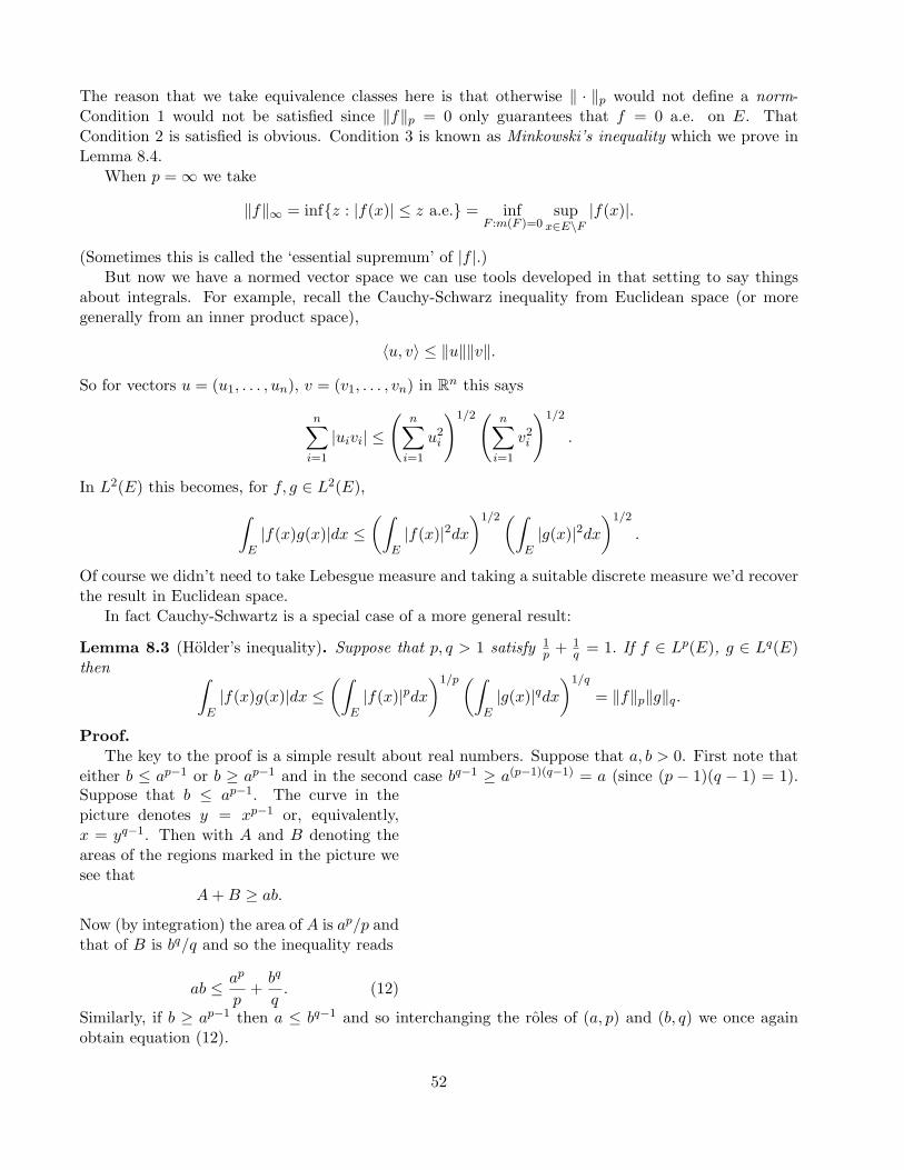
The reason that we take equivalence classes here is that otherwise ‖ · ‖p would not define a norm-Condition 1 would not be satisfied since ‖f‖p = 0 only guarantees that f = 0 a.e. on E. ThatCondition 2 is satisfied is obvious. Condition 3 is known as Minkowski’s inequality which we prove inLemma 8.4.

When p =∞ we take

‖f‖∞ = infz : |f(x)| ≤ z a.e. = infF :m(F )=0

supx∈E\F

|f(x)|.

(Sometimes this is called the ‘essential supremum’ of |f |.)But now we have a normed vector space we can use tools developed in that setting to say things

about integrals. For example, recall the Cauchy-Schwarz inequality from Euclidean space (or moregenerally from an inner product space),

〈u, v〉 ≤ ‖u‖‖v‖.

So for vectors u = (u1, . . . , un), v = (v1, . . . , vn) in Rn this says

n∑i=1

|uivi| ≤

(n∑i=1

u2i

)1/2( n∑i=1

v2i

)1/2

.

In L2(E) this becomes, for f, g ∈ L2(E),∫E|f(x)g(x)|dx ≤

(∫E|f(x)|2dx

)1/2(∫E|g(x)|2dx

)1/2

.

Of course we didn’t need to take Lebesgue measure and taking a suitable discrete measure we’d recoverthe result in Euclidean space.

In fact Cauchy-Schwartz is a special case of a more general result:

Lemma 8.3 (Holder’s inequality). Suppose that p, q > 1 satisfy 1p + 1

q = 1. If f ∈ Lp(E), g ∈ Lq(E)then ∫

E|f(x)g(x)|dx ≤

(∫E|f(x)|pdx

)1/p(∫E|g(x)|qdx

)1/q

= ‖f‖p‖g‖q.

Proof.The key to the proof is a simple result about real numbers. Suppose that a, b > 0. First note that

either b ≤ ap−1 or b ≥ ap−1 and in the second case bq−1 ≥ a(p−1)(q−1) = a (since (p − 1)(q − 1) = 1).Suppose that b ≤ ap−1. The curve in thepicture denotes y = xp−1 or, equivalently,x = yq−1. Then with A and B denoting theareas of the regions marked in the picture wesee that

A+B ≥ ab.

Now (by integration) the area of A is ap/p andthat of B is bq/q and so the inequality reads

ab ≤ ap

p+bq

q. (12)

Similarly, if b ≥ ap−1 then a ≤ bq−1 and so interchanging the roles of (a, p) and (b, q) we once againobtain equation (12).

52

Now for p > 1 take

a =|f(x)|‖f‖p

, b =|g(x)|‖g‖q

.

Then using equation (12) and integrating over E we find∫E

|f(x)g(x)|‖f‖p‖g‖q

dx ≤ 1p‖f‖pp

∫E|f(x)|pdx+

1q‖g‖qq

∫E|g(x)|qdx =

1p

+1q

= 1.

Rearranging gives the result. 2

Now let’s check the triangle inequality for Lp spaces.

Lemma 8.4 (Minkowski’s inequality). For p ≥ 1,

‖f + g‖p ≤ ‖f‖p + ‖g‖p.

Proof. The result is clear for p = 1, so suppose that p > 1. Then

‖f + g‖pp =∫E|f(x) + g(x)|pdx

≤∫|f(x)| · |f(x) + g(x)|p−1dx+

∫|g(x)| · |f(x) + g(x)|p−1dx

≤(∫|f(x)|pdx

)1/p

·(∫|f(x) + g(x)|(p−1)qdx

)1/q

+(∫|g(x)|pdx

)1/p

·(∫|f(x) + g(x)|(p−1)qdx

)1/q

where 1p + 1

q = 1 and we have used Holder’s inequality to obtain the last line. Now q(p − 1) = p andso this becomes

‖f + g‖pp ≤ ‖f‖p · ‖f + g‖p/qp + ‖g‖p · ‖f + g‖p/qp .

Finally, since p(1− 1/q) = 1, dividing both sides by ‖f + g‖p/qp we obtain

‖f + g‖p ≤ ‖f‖p + ‖g‖p

as required. 2

Much of the motivation for introducing the Lebesgue integral was its stability under limits and thatis inherited by the Lp spaces. From the point of view of an analyst a key property of Lp spaces is thatthey are complete. What this means is that every Cauchy sequence of functions in Lp converges to alimit in Lp - just as every Cauchy sequence in R converges to a limit in R. Often in analysis one definesa function through a limiting procedure and it cannot be written down explicitly. This result gives usthe power to control the behaviour of the limit.

Proposition 8.5. For 1 < p <∞, Lp is complete.

The result is still true for p =∞ but we omit the proof here.Proof of Proposition 8.5.

Let fnn≥1 be a Cauchy sequence in Lp. That is, given ε > 0 there exists N so that n,m > Nimplies ‖fn − fm‖p < ε. By passing to a subsequence if necessary we can assume that

‖fn − fn+1‖ <12n.

53

Let

gk =k∑j=1

|fj+1 − fj |, g =∞∑j=1

|fj+1 − fj |.

By the iterated Minkowski inequality ‖gk‖p < 1. By Fatou’s Lemma,

‖g‖pp =∫

limk→∞

gpk(x)dx ≤ lim infk→∞

∫gpk(x)dx ≤ 1.

So g is finite a.e. and

f = f1 +∞∑n=1

(fn+1 − fn) = limk→∞

fk

is absolutely convergent a.e. (c.f Corollary 5.30). Define f arbitrarily where the series does not converge(recall that a function in Lp is only defined up to a null set).

If ε > 0 there exists N so that ‖fn − fm‖p < ε for n,m ≥ N so for each m > N∫|f(x)− fm(x)|pdx =

∫limk→∞

|fk(x)− fm(x)|pdx

(Fatou) ≤ lim infk→∞

∫|fk(x)− fm(x)|pdx ≤ εp.

So f − fm ∈ Lp with ‖f − fm‖p ≤ ε and hence f = (f − fm) + fm ∈ Lp as required. 2

Example 8.6. Show that(m+ n)! ≤

√(2m)!(2n)!.

Solution. ∫ ∞0

xm+ne−xdx =∫ ∞

0xme−x/2xne−x/2dx

≤(∫ ∞

0x2me−xdx

)1/2(∫ ∞0

x2ne−xdx

)1/2

=√

(2m)!√

(2n)!.

2

Useful Reading

[1] H. Lebesgue Lecons sur l’integration et la recherche des fonctions primitives. Gauthier-Villars,Paris 1904.

[2] M. Capinski & P.E. Kopp Measure, Integral and Probability. Springer 2004.

[3] E.M. Stein & R. Shakarchi Real Analysis: Measure Theory, Integration and Hilbert Spaces.Princeton Lectures in Analysis III. Princeton University Press 2005.

[4] H.L. Royden Real Analysis. 3rd Edition. Macmillan 1988.

[5] R.G. Bartle The Elements of Integration. Wiley 1966.

[6] D.S. Kurtz & C.W.Swartz Theories of Integration. Series in Real Analysis Vol.9. World Scien-tific 2004.

[7] G. Temple The structure of Lebesgue integration theory. Oxford Clarendon Press 1971.

54