part i: fem –the basic idea€¦ · part i: fem –the basic idea. mae 323: lecture 2...
TRANSCRIPT
Fundamentals and ProceduresMAE 323: Lecture 2
2011 Alex Grishin 1MAE 323 Lecture 2 Fundamentals and Procedures
Part I: FEM – The Basic Idea

Fundamentals and ProceduresMAE 323: Lecture 2
2011 Alex Grishin 2MAE 323 Lecture 2 Fundamentals and Procedures
Matrix Structural Analysis (MSA):
•Legacy Structural Methods : The immediate advantage of the MSA
developed by Duncan and Collar was that one could now estimate structural
behavior for much more complex systems than was possible before. The key
to making this work lay in the assumption(s) used to connect the structural
primitives together. Historically, there were two options:
1. The Flexibility or Force Method (FM), in which forces (fe) and
moments are the primary variables of interest. In this method, you
assemble structural members, or “elements” according to:
2. The Direct Stiffness Method (DSM), in which displacements (de) are
the primary variable of interest. In this method, you assemble
structural members according to:
e e e eE= +d Q f d
e e e eE= +f K d f
e e e
e e
= +∑ ∑Q f d d where
e e e
e e
= +∑ ∑K d f f where

Fundamentals and ProceduresMAE 323: Lecture 2
2011 Alex Grishin 3MAE 323 Lecture 2 Fundamentals and Procedures
•Legacy Structural Methods (Cont.) :
Symbol Meaning
ed
eK
ef
eQ
eEd
eEf Element external force while de=0
Element external displacement while fe=0
Element internal forces
Element internal displacements
Element flexibility matrix
Element Stiffness matrix
The Stiffness Method (DSM) eventually “won”*, and still provides the
rationale for the algebraic matrix assembly today. The major advance
in today’s structural FE codes lies in how Ke is calculated (in fact, this
may be thought of as a major distinguishing feature of FEM)
*For a fascinating account of this history, see http://www.colorado.edu/engineering/CAS/Felippa.d/FelippaHome.d/Publications.d/Report.CU-CAS-00-13.pdf

Fundamentals and ProceduresMAE 323: Lecture 2
2011 Alex Grishin 4MAE 323 Lecture 2 Fundamentals and Procedures
Example 1 – Linear Springs (Pre-FEM):
•Let’s look at a simple example of Matrix Structural Analysis (MSA – here used
generically to refer to numerical structural analysis before FEM) to develop
some of the key themes which we will revisit later in the course
u1,F1
u2,F2
1
2
kx
yWe’ll start by considering a one-
dimensional spring which can
elongate in only one direction (it’s
length, which is parallel to the x-
axis).
Apply force in positive X-
direction at location 2
Fix deflection
u=u1 at location 1
Hooke’s Law states that the
springs extension, ∆u =(u2-u1)
should be equal to the spring
constant k, times force F

Fundamentals and ProceduresMAE 323: Lecture 2
2011 Alex Grishin 5MAE 323 Lecture 2 Fundamentals and Procedures
Example 1 (Cont.):
•Now let’s calculate the reaction force, F1 at location 1
•By Newton’s Third Law, we should have:
x
y
OR:
F1+F2=0 or F1=-F2
F1=-∆u x k
F1=k (u1-u2)
•A note on the color coding: Green
refers to fixed (known) displacements
while red refers to fixed (known)
forces
(1)
u1,F1
u2,F2
1
2
•Note in particular the relation of the
sign of F1 to sign of the extension, ∆u.
This is a convention we will use to add
springs to this system and not get lost
in bookkeeping (keeping track of signs)

Fundamentals and ProceduresMAE 323: Lecture 2
2011 Alex Grishin 6MAE 323 Lecture 2 Fundamentals and Procedures
Example 1 (Cont.):
•Let ‘s use what we’ve learned and apply it to a series of three springs
x
y•The fixed end implies that we have set u0=0.
Since this displacement is zero, we just
eliminate it from subsequent calculations
•Start by calculating the sum of forces
at location 1:u1
u2
u3,F3
k2
k1
k3
1
2
3u1
k1
k2
u2
1f
e
2f
e x∑F @ 11 2 1 1 2 1 2
: f f ( ) 0e e
k u k u u+ = + − =
•It will be the sum of forces associated
with extension u1 (represented by )
and u2-u1 (represented by )

Fundamentals and ProceduresMAE 323: Lecture 2
2011 Alex Grishin 7MAE 323 Lecture 2 Fundamentals and Procedures
Example 1 (Cont.):
•Proceed in the same way to calculate forces at locations 2 and 3:
x
y
k2
k3
u2
2 3 2 2 1 3 2 3: f f ( ) ( ) 0
e ek u u k u u+ = − + − =
3 3 3 23: f ( )
ek uF u= = −
x∑F @ 2
x∑F @ 3
u3,F3

Fundamentals and ProceduresMAE 323: Lecture 2
2011 Alex Grishin 8MAE 323 Lecture 2 Fundamentals and Procedures
Example 1 (Cont.):
•We now have three equations and three unknowns:
2 2 1 3 2 3( ) ( ) 0k u u k u u− + − =
3 3 2( )k u u− =F3
1 1 2 1 2( ) 0k u k u u+ − =
•This can be written in matrix form:
1 2 2 1
2 2 3 3 2
33 3 3
0 0
0
0
k k k u
k k k k u
k k u
+ −
− + − =
− F
(2)
Fundamentals and ProceduresMAE 323: Lecture 2
2011 Alex Grishin 9MAE 323 Lecture 2 Fundamentals and Procedures
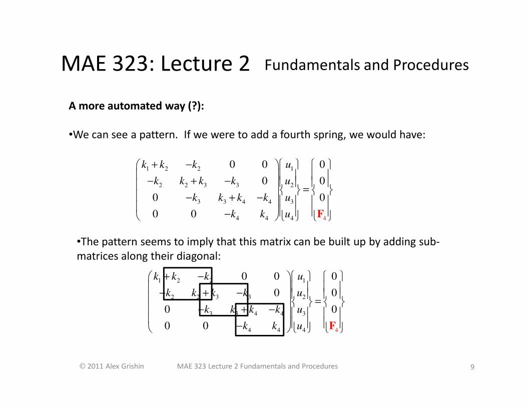
A more automated way (?):
•We can see a pattern. If we were to add a fourth spring, we would have:
4
1 2 2 1
2 2 3 3 2
3 3 4 4 3
4 4 4
0 0 0
0 0
0 0
0 0
k k k u
k k k k u
k k k k u
k k u
+ −
− + − = − + − − F
•The pattern seems to imply that this matrix can be built up by adding sub-
matrices along their diagonal:
4
1 2 2 1
2 2 3 3 2
3 3 4 4 3
4 4 4
0 0 0
0 0
0 0
0 0
k k k u
k k k k u
k k k k u
k k u
+ −
− + − = − + − − F

Fundamentals and ProceduresMAE 323: Lecture 2
2011 Alex Grishin 10MAE 323 Lecture 2 Fundamentals and Procedures
A more automated way(Cont.):
•And let’s look at one of the sub-matrices:
•This represents the spring k2 detached from the system
2 2 1
2 2 2
0
0
k k u
k k u
− =
−
u1
u2
1
2
k2
•This is equivalent to a linear longitudinal spring element
(though we didn’t use FEM to derive it)!* It has no
boundary conditions (that’s why the matrix is singular)
and no external loads, but it is ready to receive both
•For example, if we want to fix u1=0, we would strike out
(eliminate) the first row and column. If we want to add a
force at location 2, we simply place the force value in the
bottom entry of the column vector on the RHS
*In fact, let the student beware! We haven’t DERIVED anything. We’ve only made a very
clever observation (the kind engineers make) to help understand a very useful concept

Fundamentals and ProceduresMAE 323: Lecture 2
2011 Alex Grishin 11MAE 323 Lecture 2 Fundamentals and Procedures
A more automated way (Cont.):
•Let’s re-construct the matrix equation (2) knowing what we’ve learned
•We’ve got three element equations, one for each spring:
•We’ll deal with the boundary condition in the next step…
u0
u1
0
1
k1
01 1
1 1 1
0
0
k k
k k u
u− =
−
u1
u2
1
2
k2
u2
u3,F3
2
3
k3
2 2 1
2 2 2
0
0
k k u
k k u
− =
−
3
3 3
3 2
3 3
0k k u
k k u
− =
− F

Fundamentals and ProceduresMAE 323: Lecture 2
2011 Alex Grishin 12MAE 323 Lecture 2 Fundamentals and Procedures
A more automated way (Cont.):
•Now, add the matrices according to the following formula:
1. Initialize an n x n matrix with zeroes (where n is the number of locations in the series.
Also initialize an n x 1 displacement and force vector
2. Place all displacement variables into their associated location in the initialized
displacement vector (the mapping of indices is arbitrary but you must be consistent)
3. Add the element matrices to the initialized matrix such that each component
corresponds to it’s proper location w/r to the displacement vector (for example, if u2
corresponds to the third row of the displacement vector, then all entries associated with
u2 go in the third row and third column)
4. Add all the force vectors (if any) to the initialized force vector according to the same
principle
5. Eliminate all rows and columns associated with zero fixed displacements
3
0
1
2
u
u
u
u 3
0
0
0
F
1 1
1 1
k k
k k
−
− 2 2
2 2
k k
k k
−
− 3 3
3 3
k k
k k
−
−
=+
+0
00
0
0 0
Fundamentals and ProceduresMAE 323: Lecture 2
2011 Alex Grishin 13MAE 323 Lecture 2 Fundamentals and Procedures
x
y u1,F1
1
2u2,F2
X X
( ) bu x ax= +
du Fa
dx EAε = = =
Linear deflection
Linear elasticity
Ax-x=A Constant Area
(3a)
(4a)
(5)L
FE c
Aσ ε= = =
Constant strain(6a)
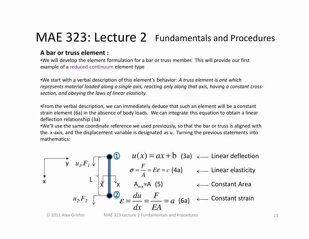
A bar or truss element :•We will develop the element formulation for a bar or truss member. This will provide our first
example of a reduced-continuum element type
•We start with a verbal description of this element’s behavior: A truss element is one which
represents material loaded along a single axis, reacting only along that axis, having a constant cross-
section, and obeying the laws of linear elasticity.
•From the verbal description, we can immediately deduce that such an element will be a constant
strain element (6a) in the absence of body loads. We can integrate this equation to obtain a linear
deflection relationship (3a)
•We’ll use the same coordinate reference we used previously, so that the bar or truss is aligned with
the x-axis, and the displacement variable is designated as u. Turning the previous statements into
mathematics:

Fundamentals and ProceduresMAE 323: Lecture 2
2011 Alex Grishin 14MAE 323 Lecture 2 Fundamentals and Procedures
2 1
1
( )( )
u uu x x u
L
−= +
2 1( )
=u udu F
dx EA Lε
−= =
Linear deflection
Linear elasticity
Constant strain
(3b)
(4b)
(6b)
•We can solve for the coefficients a and b in equation
(3) because we know that u(x)=u1 at node 1 (x=0) and
u(x)=u2 at node 2 (x=L)
•Thus, a=(u2-u1)/L and b=u1
•So, substituting these into equations (3a) , (4a), and
(6a):
2 1( )
F Eu u
A Lσ = = −Note:
We have also assumed that
no body loads exist for this
element
u1,F1
1
2
u2,F2
y
x
A bar or truss element :
•Like the spring element, the truss element has only two nodes and two DoF’s. We
know that it has a linear displacement field (equation (3a)), but we need a local
coordinate reference for this equation. The coordinate system we have been using was
a global reference. For the local reference, we’ll just translate the global reference and
set x=0 to coincide with node 1. We will call this the element coordinate system.

Fundamentals and ProceduresMAE 323: Lecture 2
2011 Alex Grishin 15MAE 323 Lecture 2 Fundamentals and Procedures
A bar or truss element :
•Now, multiplying equation (4b) by A, yields:
2 1( )
EAF u u
L= −
•And , equation (6b) tells us that (u2-u1)/L (the strain) is constant.
So, over a truss element of length L , we can recover Hooke’s
Law:EA
F u k uL
= ∆ = ∆
•So, the truss element has constant stiffness:
EAk
L=
•From our work with springs, this implies the
element equilibrium equation must be:
1 1
2 2
1 1
1 1
u FEA
u FL
− =
−
(7)
(8)

Fundamentals and ProceduresMAE 323: Lecture 2
2011 Alex Grishin 16MAE 323 Lecture 2 Fundamentals and Procedures
•This produces an equation of the form:
1 2( ) 1
x xu x u u
L L
= − +
1
( ) ( )n
e
i i
i
u x N x u=
=∑Where n is the order of the polynomial used to
approximate the solution and are the nodal
solution values for element e
e
iu
(8)
•Equation (8) is defined only over the element support (in this case, x1≤x≤x2)
defined by nodes 1 and 2 (it is zero elsewhere). This makes it a piecewise
polynomial. The functions, Ni are called shape functions. They are very useful in
determining the solution anywhere in an assembled structure (not just nodes).
Because of displacement compatibility at nodes (referred to in the literature as C0
continuity), we can use (9) to construct an interpolating displacement field over the
entire structure as:
(9)
1
( ) ( )nx
i i
i
u x N x u=
=∑ (10)
A bar or truss element :
•Finally, if we collect terms involving u1 and u2 in equation (3b):

Fundamentals and ProceduresMAE 323: Lecture 2
2011 Alex Grishin 17MAE 323 Lecture 2 Fundamentals and Procedures
1 2 3
•Here’s a curve generated by equation (10) with c={1,2,5} and the shape
functions, N above:
L
L
A bar or truss element (Cont.) :
•Shown below are the shape functions of two truss elements which share a node
(node 2):
1
2N
1
1N
2
2N
2
1N

Fundamentals and ProceduresMAE 323: Lecture 2
2011 Alex Grishin 18MAE 323 Lecture 2 Fundamentals and Procedures
A bar or truss element (Cont.) :
•But this truss element is confined to coordinate directions parallel to it’s length
•In order to account for more arbitrary orientations, we need to perform a coordinate
transformation
x
y
x
y
θ •The element coordinate system (x’-y’) makes a an
angle, θ with the global (x-y) . Let u be the deflection
in the x-direction and v be the deflection in the y-
direction.
•The element deflections and node 1 and 2 in the
primed coordinate system are:
u1
v1
u2
v2
'
1 1 1cos sinu u vθ θ= +
'
2 2 2cos sinu u vθ θ= +
•Now, to simplify notation, we make
the substitution:
cos
sin
c
s
θ
θ
=
=
(11)
1
2

Fundamentals and ProceduresMAE 323: Lecture 2
2011 Alex Grishin 19MAE 323 Lecture 2 Fundamentals and Procedures
A bar or truss element (Cont.) :
•Now, re-write (11) in vector-matrix notation as:
' =u Rd
Where d is the displacement vector in global coordinates and R is the
“global-to-local” rotation matrix. Expanding this yields:
1
'
11
'
22
2
0 0
0 0
u
vc su
uc su
v
=
•This transformation can be used to represent the element equilibrium
in any arbitrarily orientated global coordinate system as:*
( ' )
e e eor
=
=
TR k R d f
k d f
*This represents a tensor rotation, which can be derived by at least two methods. For
details, see:
T. Yang, Finite Element Structural Analysis. Prentice-Hall, Inc., 1986.
(12a)

Fundamentals and ProceduresMAE 323: Lecture 2
2011 Alex Grishin 20MAE 323 Lecture 2 Fundamentals and Procedures
A bar or truss element :
•Expanding (12a) results in the full matrix equation for an arbitrarily oriented truss
element :
2 211
2 211
2 222
2 222
x
y
x
y
Fuc cs c cs
Fvcs s cs sEA
FuL c cs c cs
Fvcs s cs s
− −
− − = − − − −
•Note that we have gone from an element with 2 DoF’s to 4 (even
though the element doesn’t behave any differently)
•The same transformation works for spring elements (simply replace
EA/L by k. A similar process may be used to transform spring and truss
elements into a 3D space
•These element equations are now in a form ready to be assembled into
a global system via the technique (DSM) we have already seen
(12b)

Fundamentals and ProceduresMAE 323: Lecture 2
2011 Alex Grishin 21MAE 323 Lecture 2 Fundamentals and Procedures
What else is there? :
•Actually, there’s a lot more. For now, the student should be aware that any numerical
procedure in mechanics involves “discretizing” an equation in order to approximate
solutions to it at discrete points. This means the domain must be split into finite pieces,
or elements. This is called meshing in the literature. Methods of doing this in an
automated way are not trivial and will be discussed in future lectures
•Equation (8) and (12) were derived according to the “Direct Method”*. In other words,
the element matrices were derived based on our pre-existing knowledge of the solution
to the associated differential equations. Many element types encountered in structural
analysis may be obtained this way. For example, an Euler-Bernoulli beam element may
be derived this way (for details see the reference below):
•Without actually giving the derivation, we will present the element stiffness matrix for
the Euler-Bernoulli beam element with DoF’s shown below
* R. Cook, D. Malkus, and M. Plesha, Concepts and Applications of Finite Element Analysis,
3rd ed. New York, NY, USA: John Wiley & Sons, 1989.
1 2
v1,y
x
v2
θ2θ1

Fundamentals and ProceduresMAE 323: Lecture 2
2011 Alex Grishin 22MAE 323 Lecture 2 Fundamentals and Procedures
The Euler-Bernoulli Beam Element :
•The equilibrium equation for the Euler-Bernoulli beam element:
1 1
2 2
1 1
3
2 2
2 2
2 2
12 6 12 6
6 4 6 2
12 6 12 6
6 2 6 4
e e e
v FL L
ML L L LEI
v FL LL
ML L L L
θ
θ
−
− = = = − − − −
k d f
•We can further augment this beam element to include extensions (truss
behavior) by adding the two DoF’s from the truss element as follows:
1
1
2 2
1
3
2
2
2 2
2
1 0 0 1 0 0 0 0 0 0 0 0
0 0 0 0 0 0 0 12 6 0 12 6
0 0 0 0 0 0 0 6 4 0 6 2( )
1 0 0 1 0 0 0 0 0 0 0 0
0 0 0 0 0 0 0 12 6 0 12 6
0 0 0 0 0 0 0 6 2 0 6 4
e e e e
T B
u
vL L
L L L LAE EI
uL L
vL L
L L L L
θ
θ
−
− −
+ = = + −
− − − −
k k d f
1
1
1
2
2
2
x
y
x
y
F
F
M
F
F
M
=
(13)

Fundamentals and ProceduresMAE 323: Lecture 2
2011 Alex Grishin 23MAE 323 Lecture 2 Fundamentals and Procedures
Part II: The Procedure

Fundamentals and ProceduresMAE 323: Lecture 2
2011 Alex Grishin 24MAE 323 Lecture 2 Fundamentals and Procedures
•Every finite element analysis consists of the following steps
1. Formulation of Physical Problem
2. Analysis Type Selection
3. Physical Reduction (Idealization)
4. Element Type Selection
5. Model Creation
a) Loads and Boundary Conditions
b) Material Properties
c) Mesh
6. Solution
7. Post-processing
8. Validation

Fundamentals and ProceduresMAE 323: Lecture 2
2011 Alex Grishin 25MAE 323 Lecture 2 Fundamentals and Procedures
1. Formulation of the Physical Problem
•In the case of MAE 323, this is a slam-dunk, because we will always be
performing a linear static thermal, structural, or thermal/structural
problem
•However, the student should note that in general, this isn’t always as
obvious as it seems. The questions that must answered here include:
•What forces are involved?
•By what mechanism is energy dissipated? Remember, in our case
it’s always some variant of Hooke’s Law. This will always reveal
the constitutive law(s)
•Is the problem linear or nonlinear?
•Is the problem time-dependant?

Fundamentals and ProceduresMAE 323: Lecture 2
2011 Alex Grishin 26MAE 323 Lecture 2 Fundamentals and Procedures
1. Formulation of the Physical Problem
•As an example, suppose your boss (or customer) asks you to perform
a vehicle crash study. At first, you may be (rightly) bewildered. Start
by answering the questions on the previous slide:
•What forces are involved? Mostly momentum-driven impacts of
the form F=-m∆V/∆t
•By what mechanism is energy dissipated? Mostly mechanical
deformation and damping
•Is the problem linear or nonlinear? Highly nonlinear
•Is the problem time-dependent? Yes

Fundamentals and ProceduresMAE 323: Lecture 2
2011 Alex Grishin 27MAE 323 Lecture 2 Fundamentals and Procedures
2. Analysis Type Selection
•In the case of the vehicle crash study, answering the
questions in the last step reveals that we have to do a
nonlinear-transient time-history study
•Once we have determined the physical formulation (which should
emerge naturally from answering the previous questions), we
determine what analysis type is to be performed. This is like making a
selection from a menu. The analyst has to be aware which finite
element solver/element-type combinations exist in order to match
the physical formulation with a finite element procedure capable of
approximating it . This may not be easy, and in many cases may
amount to asking “Does our commercial software product have this
capability?”

Fundamentals and ProceduresMAE 323: Lecture 2
2011 Alex Grishin 28MAE 323 Lecture 2 Fundamentals and Procedures
•Even in the case of problems in MAE 323 (all physics may be characterized as
thermal/mechanical elastostatics), questions will arise as to whether the
problem may be best characterized as a full continuum, reduced continuum
(dominated by bending or membrane behavior), spring connections, or a
combination of all three
•This problem is multiplied when we consider the analysis of assemblies (as
you often will in your professional careers). In many cases, you often analyze
for predefined performance points. For example, a pressure regulator will be
analyzed for predefined (design) pressure conditions which represent either
typical or extreme performance conditions (more about that in later
lectures). The analyst has to make assumptions about the load paths in each
of these conditions, and these will determine how the model is built (and
how many models must be built!)
3. Physical Reduction (idealization)

Fundamentals and ProceduresMAE 323: Lecture 2
2011 Alex Grishin 29MAE 323 Lecture 2 Fundamentals and Procedures
4. Element Type Selection
•Element types may be categorized in terms of:
•The physical field they approximate (in our case, it will always be
material displacement or temperature)
•The type of field behavior: continuum, multiple-continuum
(coupled field), mixed-variable(for example, in hyper-elastic
applications), reduced continuum, or special connection (such as
contact elements, but more on these in later lectures)
•So back to the vehicle-crash example: the engine-block and other internal
heavy components may be modeled as full-continuum or mass-elements,
depending on whether we care about stresses and strains in those
components. If we don’t, then we just need to model the mass and possibly
use special elements to connect the mass to the components we DO care
about. What we care about mostly is the chassis and body. The mechanical
behavior of these components will most certainly be dominated by bending
(and eventually buckling and crumpling), and thus we should use shell
elements for the body and possibly beams for the chassis

Fundamentals and ProceduresMAE 323: Lecture 2
2011 Alex Grishin 30MAE 323 Lecture 2 Fundamentals and Procedures
•Finally, the vehicle will impact another object – maybe another vehicle or
something stationary – so contact must be defined between the vehicle surfaces
and what the vehicle will impact. At the basic mathematical level, contact is
treated as an additional (nonlinear) constitutive law which connects element
surfaces with either a penetrability condition, or some other law relating how the
surfaces move relative to one another. We refer here to contact between
impacting surfaces, but that is just one type of contact or special connection we
might define. For example, we might use rotational springs, or DoF couples to
attach the doors, hood, and trunk to the chassis. Numerically, there are several
ways to impose such a condition. Some commercial software does so with special
elements (and others simply add the appropriate matrix terms to the assembled
system matrices internally). This (contact) is a very large topic and the details are
handled many different ways by different commercial software

Fundamentals and ProceduresMAE 323: Lecture 2
2011 Alex Grishin 31MAE 323 Lecture 2 Fundamentals and Procedures
5. Model Creation
•With all the previous selections out of the way, we can begin building the
model…a) Loads and Boundary Conditions: The choices made in steps 2 and 3 dictate
where and how the loads and boundary conditions will be distributed. In
the case of our example, one vehicle/object might be fixed (stationary) or
free-free but motionless (In some types of solvers, you would need to attach
light springs to such an object to prevent matrices from becoming singular.
Other types don’t require this). The other vehicle would have an initial
velocity imposed upon it
b) In MAE 323, the materials will usually be well-defined. However, in highly
nonlinear applications, the choices get more difficult. For example, in the
vehicle crash study, we will probably need not only the full stress/strain
curves (obtained from tensile tests), but also strain-rate behavior (hard to
come by)
c) We can now mesh the model. We need to know what type and size mesh we
need (more on this topic in the next lecture). In our case, let’s say we’ve
settled on a quadrilateral mesh for the shells (body), and tetrahedra for solid
internals. Most commercial software can automatically mesh these bodies,
but some of our connections may require manual construction

Fundamentals and ProceduresMAE 323: Lecture 2
2011 Alex Grishin 32MAE 323 Lecture 2 Fundamentals and Procedures
5. Solution
•Solvers are generally categorized by exactly how the system
equations are solved. In the vehicle crash example, options include
implicit vs. explicit time-integration, sparse vs. iterative, etc. Vehicle
crash studies usually involve very short timeframes (relative to the
period of the system natural frequencies), and thus explicit solvers
are usually used (these have other enormous advantages, but the
discussion takes us too far from the class goals)
6. Post-processing
•In this step, the user has to extract the metrics of the material
response. These are usually in the form of displacement, stress, and
strain contour plots at a given time in the solution (or temperature in
the case of thermal analyses). But in our example, we might also want
accelerations and velocities at specific points (nodes). These would be
in the form of tables (vs. time)

Fundamentals and ProceduresMAE 323: Lecture 2
2011 Alex Grishin 33MAE 323 Lecture 2 Fundamentals and Procedures
7. Validation
•Much can go wrong in an analysis. Not only can we impose incorrect
boundary conditions and loads, but we might have constructed the
mesh so poorly that it yields incorrect results (especially for derived
quantities such as stress and strain). In the case of the vehicle crash
study, we might have also chosen a numerical integration time-step
that is too large (in the case of implicit solvers), which would also yield
incorrect results, or perhaps used the wrong material properties
(maybe the density we used for the heavy internal components was
way off)
•This is why we always have to validate our models. In MAE 323, this is
much easier than the vehicle crash study offered here as an example.
We can use the techniques we learned in Lecture 1. But we can also
consult standard tables (for things like stress concentration factors) for
more complicated problems

Fundamentals and ProceduresMAE 323: Lecture 2
2011 Alex Grishin 34MAE 323 Lecture 2 Fundamentals and Procedures
A Simple Example: The Bolted Flange
•Suppose you have a pressure vessel and you want to know the
maximum (von Mises) stress at a bolted flange. To keep things simple,
we’ll already start with a simplifying assumption: Namely that the
flange around each bolt may be represented as below (pressure vessels
have many bolts):
Two mating plates
(0.5” thick) Mating
surfaces see 2000
psi pressure
Bolt
Washer 1
Washer 2Nut
Thru-
hole

Fundamentals and ProceduresMAE 323: Lecture 2
2011 Alex Grishin 35MAE 323 Lecture 2 Fundamentals and Procedures
A Simple Example: The Bolted Flange
•Let’s go through the check-list to see if we know how to model this
1. Formulation of physical problem: This is a linear static
structural problem
2. Analysis type: Linear static problems only have one analysis
type (linear static)
3. Physical Reduction: This will be a full continuum problem
because we are looking for full 3D stress fields produced by
surface interactions. There may be some geometric
simplification. For example, we don’t even have to model the
bolt if all we care about is flange stresses (more on this later)
4. Element type selection. Since this is a 3D structural continuum
problem, we can accept the workbench default element types
for this type of problem (tetrahedral solid elements with mid-
side nodes)

Fundamentals and ProceduresMAE 323: Lecture 2
2011 Alex Grishin 36MAE 323 Lecture 2 Fundamentals and Procedures
A Simple Example: The Bolted Flange
5. Model Creation
a) Loads and Boundary Conditions. The loads are simply
pressure loads on the flange surfaces. The boundary
conditions are a little more involved (we’ll discuss that
next)
b) Material Properties. In this problem, structural steel is
used for all parts
c) Mesh. The mesh will need to have enough resolution to
adequately capture the peak stresses. One way to do this
is to require a certain maximum percentage change in the
results of two successive mesh densities (eg: max. stress
must not change by more than 4 percent when reducing
element size by 50 percent)
6. Solution
We will accept default settings for now (later lectures will
address solution settings)

Fundamentals and ProceduresMAE 323: Lecture 2
2011 Alex Grishin 37MAE 323 Lecture 2 Fundamentals and Procedures
A Simple Example: The Bolted Flange
7. Post-Processing
Since this is a pressure vessel, we will want to look at both
deflections and stress (with pressure vessels, flange
separation is often of interest)
8. Validation
Since there are equal and opposite pressures on each flange
surface, we will want to ensure that the total reaction force in
the pressure direction is zero (this should be determined at
the region that is fixed in that direction). We might also want
to ensure that the reaction at each flange is P*A where P is
the pressure on that flange and A is the surface area over
which it is applied

Fundamentals and ProceduresMAE 323: Lecture 2
2011 Alex Grishin 38MAE 323 Lecture 2 Fundamentals and Procedures
A Simple Example: The Bolted Flange
Loads and Boundary Conditions
•The only thing we have not yet determined is what kind of
boundary condition this model should receive. That will require
some discussion
•First, it helps to understand something about bolted flanges.
Many books on Mechanical Engineering Design offer a
simplification* involving an estimate of how the load is transmitted
through the flanges. The simplification assumes the load is entirely
concentrated within the frustum produced by the plane of the
flange interface intersecting a hypothetical cone of a prescribed
angle, also intersected by the plane of the underside of the bolt
head
*see, for example: J. Shigley and C. Mischke, Mechanical
Engineering Design, 5th ed. McGraw-Hill, 1989.

Fundamentals and ProceduresMAE 323: Lecture 2
2011 Alex Grishin 39MAE 323 Lecture 2 Fundamentals and Procedures
A Simple Example: The Bolted Flange
Loads and Boundary Conditions
•The simplification is depicted graphically below
θ
Values of
∼30° are
typically used
for bolt load
frusta
t
db
dp
2 tanp bd d t θ= +
The flanges are
bonded only within
the frustum
diameter dp
No load is
transmitted across
these surfaces and
so no contact is
assumed

Fundamentals and ProceduresMAE 323: Lecture 2
2011 Alex Grishin 40MAE 323 Lecture 2 Fundamentals and Procedures
A Simple Example: The Bolted Flange
Loads and Boundary Conditions
•We expect the following type of material response due to the
pressure on each flange surface:

Fundamentals and ProceduresMAE 323: Lecture 2
2011 Alex Grishin 41MAE 323 Lecture 2 Fundamentals and Procedures
A Simple Example: The Bolted Flange
Loads and Boundary Conditions
•Suppose we are interested only in the stress at the bolt flange
interface (the diameter of the frustrum dp). If this is the case, we
can remove the bolt (we don’t have to model it)
•The annular region whose outer diameter is represented by dp
must still be modeled (we need a circular “patch” on the interface
with which we can define the bonded region)
dp
What kind of
boundary condition
should go on these
surfaces?

Fundamentals and ProceduresMAE 323: Lecture 2
2011 Alex Grishin 42MAE 323 Lecture 2 Fundamentals and Procedures
A Simple Example: The Bolted Flange
Loads and Boundary Conditions
•Remember, this bolted flange model already has an assumption
built into it: Namely that it is a repeated feature which reacts in the
same way (and to the same extent) as all the others
•The bolted flange model is effectively “cut” out of a larger model
(along the dotted green line above). The cut boundaries behave as
Cartesian symmetry planes
Symmetry PlaneSymmetry Plane

Fundamentals and ProceduresMAE 323: Lecture 2
2011 Alex Grishin 43MAE 323 Lecture 2 Fundamentals and Procedures
A Simple Example: The Bolted Flange
Loads and Boundary Conditions
•So, what’s a symmetry plane?
•A symmetry boundary condition is a surface on which primary solution variables
(displacement in structural models) are set to zero normal to the surface. Such a
boundary condition usually reflects a theoretical dividing line through a domain – both
sides of which behave identically. The figure below shows a planar model (one type of
symmetry), which is identically loaded at opposite ends. The geometry and loading admit
a plane of symmetry which can be used to “cut” the model in half
x
y
ux=0
Fundamentals and ProceduresMAE 323: Lecture 2
2011 Alex Grishin 44MAE 323 Lecture 2 Fundamentals and Procedures
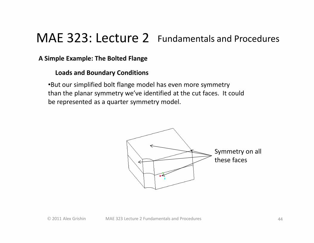
A Simple Example: The Bolted Flange
Loads and Boundary Conditions
•But our simplified bolt flange model has even more symmetry
than the planar symmetry we’ve identified at the cut faces. It could
be represented as a quarter symmetry model.
Symmetry on all
these faces