part i: observations
TRANSCRIPT

Part I: Observations
IFS DOCUMENTATION – Cy47r3
Operational implementation 12 Oct 2021
PART I: OBSERVATIONS
© Copyright 2020-
European Centre for Medium-Range Weather ForecastsShinfield Park, Reading, RG2 9AX, UK
The content of this document is available for use under a Creative Commons Attribution 4.0 InternationalPublic License. See the terms at https://creativecommons.org/licenses/by/4.0.
IFS Documentation – Cy47r3 1

REVISION HISTORY
Changes since CY43R1
• Minor change to text in subsection ’Conventional observations’.• New subsection on ’Additional error inflation for dropsondes’.
Changes since CY41R2
• Major rewrite and restructure of the observation documentation reflecting OOPS developments forCY43R1, removal of outdated material and identification of deprecated areas of code.
2 IFS Documentation – Cy47r3
Part I: Observations
Chapter 1
Overview: the observation world
Table of contents1.1 Introduction
1.2 Concepts
1.2.1 Observation groupings, reports and datums
1.2.2 Observation sets
1.2.3 Timeslots
1.2.4 Events and status
1.2.5 The screening trajectory
1.2.6 Observation Database usage in IFS
1.2.7 Parallel aspects (scalability)
1.3 Dataflow through processing and screening
1.4 Observation groupings in the IFS
1.4.1 Obstype and codetype
1.4.2 SQNO - [DEPRECATED]
1.4.3 Physical variable: varno
1.4.4 Observation operator codes: NVAR - [DEPRECATED]
1.4.5 Satgrp table and friends
1.4.6 ‘Area’ type - [DEPRECATED]
1.4.7 VarBC bias groups
1.1 INTRODUCTION
The handling of observations is one of the most complex parts of the IFS data assimilation system. Observationscome in diverse forms and, depending on their type, they are treated in very different ways. The observationsthemselves (y) and the observation operator H(), which converts from the model state x to an observationequivalent H(x), are just part of a wider infrastructure of processing, quality control, thinning, and assigningobservation errors. The metadata associated with each observation can run into hundreds of variables, allneeding to be stored in an observation database (ODB). Thus the observation world encompasses:
• Observation operators as described in Chapter 3. The input to the observation operator is the ODB,plus the the model state at observation locations. Observation operators, as well as generating H(x),may put additional information into the ODB in some cases including observation error and qualitycontrol decisions.
• Model state interpolated to observation location or GOM PLUS is described in Part 2(Data Assimilation). This contains vertical profiles of atmospheric variables (temperature, humidityetc.), surface variables and any other information required from the model. Using the ‘2D GOM’ facility,instead of a single vertical profile, the GOM PLUS can contain a slant-path, a set of profiles along alimb path (e.g. for GPSRO) or just all the nearby model columns (which is used in the Bayesian radarretrieval at Meteo-France).
• ODB is a collection of data formats and metadata describing the observations.
– In the core of the IFS, processing is based on ODB-1, a hierarchical table format capable of runningin a parallel environment, manipulated and accessed using Structured Query Language (SQL).Documentation on ODB-1 can be found at https://software.ecmwf.int/wiki/display/ODB/ODB+User+Guide.
IFS Documentation – Cy47r3 3

Chapter 1: Overview: the observation world
– However, most interactions with ODB in the IFS use an additional layer of code known as ODB-IFSwhich is in the process of being completely rewritten. See Sec. 1.2.6.
– For some pre-processing, and for archiving to MARS, the ODB-2 format is used: https:
//software.ecmwf.int/wiki/display/ODB/ODB+API.– The variables and codes used in the ODB are governed by a committee, and can be browsed at
http://apps.ecmwf.int/odbgov.– At a more detailed level, some parts of the ODB contents are described in the current
documentation, mainly in Chapter 6.
• Observation processing is a chain that leads from the ingestion of raw data (as BUFR files andother data formats) to the archiving of ODBs in MARS containing diagnostics from the assimilationrun (traditionally known as feedback files). Apart from running the observation operators in the dataassimilation, observation processing has two main components that can be described as ‘preparation’and ‘screening’, described next.
• Preparation generates all the parameters needed to run the observation operator in the assimilationsystem. This is everything from format conversions (e.g. BUFR to ODB-1) to the retrieval of surfaceemissivities or cloud top pressure from satellite radiances. It is also necessary to apply coordinatetransforms (for example from windspeed and direction to horizontal wind components) or to runa retrieval prior to assimilation (for example from backscatter to ocean surface wind). This stagemay include simple thinning (such as discarding some satellite observations) This stage also sets upobservation errors and other parameters such as the settings for quality control. All this is described inChapter 2.
• Screening includes all the decisions whether or not to use a certain data. Screening decisions aremade throughout the processing chain. They includes blacklisting and other quality control decisionsthat can only be made when a first guess is available, or in the presence of all observations (‘dependent’screening). See Chapter 4.
• Observation errors: the diagonal part of the observation error matrix R is created during observationprocessing. For conventional observations, it is done in COPE; for other observations it may be createdin DEFRUN or the first time the observation operator is called, particularly if the observation error issituation-dependent. This observation error is eventually stored in the ODB for later use by the dataassimilation system. Correlated parts of the observation error model are described in Part 2 (Dataassimilation).
• Bias correction Some bias correction is performed as part of pre-processing (such as for radiosondes,done in COPE) but most is now handled inside the 4D-Var minimisation using variational bias correction(VarBC). This is more properly part of the data assimilation, so it is also left to Part 2.
• Other auxiliary control variables Similar to VarBC, other auxiliary control variables are used forsatellite radiance assimilation. These include a skin temperature sink variable and a cloud top heightvariable, and are partly described in Part 2, but their main documentation is here, in Chapter 3.
• Variational quality control This is part of the data assimilation algorithm, so again it is found inPart 2. However, it is the responsibility of the observation processing to provide the parameters thatcontrol these tests, such as for example the Huber norm parameters; these are stored in the ODB foruse during the assimilation.
• Diagnostic Jo table Although this is another Part 2 concept, the diagnostic Jo table has a detailedstructure that breaks down observations into smaller groups, such as observation type and variable for theconventional observations (e.g. radiosonde wind) and satellite instrument for radiances (e.g. AMSU-A).This fine structuring of observations is known only by the observation world, and is described here.
As with the rest of the IFS, the observation world has built up over more than 20 years and is still in constantdevelopment. Processing takes place in different layers of code, from ancient parts of the original IFS, throughto more OOPS encapsulations. We are constantly working to remove and refactor the older layers of code,but this is an ongoing task. Many areas and concepts are now ‘deprecated’, in other words they still provideimportant functions but they are expected to disappear in future cycles and they should not be involved in newdevelopments. Where possible, this is clearly stated in the current documentation, and their descriptions havebeen moved to a special section: Chapter 5. More broadly, the exercise of documenting code is a good way tounderstanding its inadequacies and indicating ways its design could be improved; thus it also tries to identifyareas that could be rationalised in future cycles. To understand the code as it stands, it is worth knowing the
4 IFS Documentation – Cy47r3

Part I: Observations
history of such developments. For example, before the ODB was introduced, observations were stored in a datastructure called CMA, and concepts from the CMA live on in many places, some good, others outdated andin the process of being refactored. Parts of the processing for conventional observations have been exportedinto the COPE project, and the ability to call observation operators has now been encapsulated for OOPS,but areas such as setup and screening have not seen so much development.
1.2 CONCEPTS
1.2.1 Observation groupings, reports and datums
Observations are organised into a heirarchical structure which is reflected in ODB-1. At the broadest level,observations can be organised into meaningful groupings, such as the data from a sensor on one satellite,or all drifting buoys. There are a number of schemes for grouping used in the IFS, and many of thesegroupings overlap, since they make sense in some areas but not others. Lower down is the concept of a ‘report’,encompassing for example a single radiosonde ascent or a satellite observation that spans multiple frequencies.Each report thus contains multiple observations, often referred to as datums. Strictly, the plural of datumis data, but ‘datum’ or ‘datums’ emphasises that this is the lowest quantum of observational information.In the ODB each datum is associated with a vertical position (vertco reference 1@body, given in terms ofpressure, height or channel number) and a variable number (varno@body). Datums are grouped into reportsto take advantage of their common characteristics: for satellite observations, we often loosely think of thereport level as the ‘observation’; the datums in the report (measurements at different frequencies) relate toa single location and were made using the same observational parameters, such as scan angle or instrumenttemperature. Hence it is more precise to talk about datums and reports than ‘observations’.
1.2.2 Observation sets
To allow efficient parallel computation in the IFS, reports are usually processed together in a small groupsknown as sets. The maximum number of reports in a set is given by NMXLEN (yomdimo; default 511 butcurrently set to 64 by namelist). To balance the parallel processing, sets are handled in order from the mostcomputationally expensive to the least. The observation sets may span several 4D-Var timeslots, though inthe current operational context this is not the case. Sets are generated by the class OBSOP SETS withtheir detailed organisation being handled by ECSET. Satellite observation sets (e.g. radiances, AMVs, limbradiances, scatterometer) must not contain data from more than one instrument. This is controlled by themisnamed ‘area’ parameter, which for radiance data is an indicator of satellite ID and instrument, determinedin SUOBAREA.
1.2.3 Timeslots
Timeslots are sub-divisions of the 4D-Var window into which observations are grouped for processing, typicallyof length 30 minutes. For interpolation from model to observation space, one timestep of the model is chosen torepresent the model state in that timeslot. Timeslots are useful because they isolate the observation groupingfrom the model time resolution, which varies within 4D-Var. However, timesteps may be eliminated in futureto simplify the code and to use the most appropriate model timestep for the observation.
1.2.4 Events and status
The results of observational processing are stored in the ODB, at the report and datum level, in columnscalled REPORT STATUS, DATUM STATUS, REPORT EVENT1 and DATUM EVENT1 (Secs. 6.8 and 6.9).The status summarises whether (and how) the observations should be used in the assimilation system; theevent columns are bitfields that record the causes of data rejection, plus some other processing events. Manyprocessing decisions are unique to a particular observation type. For this reason, the REPORT EVENT2 andDATUM EVENT2 columns can be customised according to the observation type, although in practice thisfacility is rarely used. All-sky radiance observations use their own event bitfield called DATUM TBFLAG(Sec. 3.3.3).
IFS Documentation – Cy47r3 5
Chapter 1: Overview: the observation world
1.2.5 The screening trajectory
Most observations rely on the ‘screening trajectory’ to perform one-off initialisations that may require themodel’s first guess. Hence a large part of the observation processing runs only once, in the pre-processingchain, or in the first trajectory under the screening flag LSCREEN = .TRUE. This leads to some confusionover what ‘screening’ means. This documentation makes the distinction between ‘preparation’ (some of whichtakes place when the screening is being done, but is not screening) and true screening, which selects data togo into the assimilation algorithm, and is applied at or after the stage the observation operator is run.
1.2.6 Observation Database usage in IFS
ODB-1 is an MPI-parallel distributed in-memory, hierarchical database developed at ECMWF. The IFS usesODB-1 to access observational data and store feedback data (for example, to store first guess departures andinformation on whether a particular observation was rejected by screening).
Typically, when IFS needs to access observational data, an SQL query is run to retrieve a subset of the data.The queries themselves can be found in the odb/ddl directory. The results from the query are returned in 2Darrays. The IFS then uses and manipulates these data arrays, before the modified data is put back into theODB again. Often, separate queries are run for the report-level data (stored in ROBHDR) and the datum-leveldata (stored in ROBODY). In a typical screening trajectory, each MPI tasks performs O(10,000) separate SQLqueries on the database.
Although IFS uses ODB-1, there are no direct calls to the ODB library from the IFS source code. Instead, IFSaccesses ODB through an interface layer. The original IFS-ODB interface is contained in the odb/cma2odbdirectory. Subroutines such as GETDB() and PUTDB() wrap up the lower level ODB get() and ODB put()library calls, and perform other tasks such as setting up column index variables.
An improved, IFS-ODB interface layer (named ifsobs) is being developed. While the old interface relied heavilyon global variables and C pre-processor macros, the new interface is more modern and flexible, taking advantageof the object-oriented features of Fortran 2003. The new interface provides more transparency on what SQLsare being run, and which columns are being accessed (aspects which were previously obscured). It also hasthe advantage that it allows for other database backends to be plugged in seamlessly. The new ifsobs-basedinterface is in the process of being rolled out in IFS, and in CY43R1 is confined to the observation operatorcode.
1.2.7 Parallel aspects (scalability)
The IFS is multi-process multi-threaded parallel. For running the forecast model, each process holds thestate variables for a small part of the globe. In contrast observations are (roughly randomly) distributedacross all processors with the aim of avoiding any geographical link. Each processor works with a selection ofobservations from across the globe. This is why the interpolation from model space to observation space (theGOMs) is one of the more demanding parallel-processing tasks in the IFS. An alternative strategy of keepingthe relevant observations on the processor that owns the model data would fall down in two ways: First, ahorizontal interpolation, and even more so a limb or slant path interpolation, will often need access to modeldata located on multiple processors, so multi-process communication would be needed anyway. Second, thecomputational burden would be unequally distributed, concentrated in whichever processors have satellitesoverhead on that particular timestep: maybe a dozen out of hundreds.
The top level for running the observation operator is TASKOB (or its tangent-linear and adjoint equivalents)which loops over the available observation sets on that processor. This loop is multi-threaded, which meansthat many sets will be processed in parallel. Moreover, given that the IFS is also multi-process parallel, eachprocessor will be handling different sets of observations. Running the observation operator is thus almostperfectly scalable, as long as the workload is evenly distributed across all processors and threads.
The next level down is TASKOB THREAD which handles the parallel parts of the observation loop. For eachobservation set, it calls YDGOM5%MODEL AT OBS to get the GOM PLUS (the model state at observationlocations) and then calls the per-set observation operator HOP, which is where Chapter 3 (Observationoperators) takes over. The screening uses a similar framework of a parallel loop over observation sets.
6 IFS Documentation – Cy47r3

Part I: Observations
STATE INDEPENDENT PREPARATIONS
ODB-1
SUPPORT DATA
PREPARATIONS (INCLUDING STATE DEPENDENT)
FORECAST SUPPORT DATA
ODB-1
SCREENING OF OBSERVATIONSFORECAST SUPPORT DATA
FORECAST SUPPORT DATA
ODB-1ANALYSIS
4DVAR ANALYSIS
LEGEND
OBSERVATIONS
DEPARTURES/FLAGS (FG)
MODEL FIELDS
SUPPORT DATA
ESTIMATED PARAMETERS
HIGH LEVEL TASK
LOW LEVEL TASK
DEPARTURES/FLAGS (AN)
ODB-1
SAT BUFR CONV BUFR CONV TAC
Figure 1.1 Simplified IFS observation processing flow diagram, with the disc icons representing datastores and the rectangles representing processing stages. Further details can be found in Fig. 2.1 for thestate-independent preparations, Fig. 2.2 for the main preparations, Fig. 4.1 for the screening and Fig. 3.1for 4D-Var.
1.3 DATAFLOW THROUGH PROCESSING AND SCREENING
Observation processing happens at many different stages during the journey through the IFS. For computationalreasons it can be helpful to reduce observation numbers early on, when the data is stored compactly, andbefore too much computational time has been expended on unwanted data. However, the cost of observationprocessing in the current operational system is small, and these computational limitations are not as importantas they have been (Lean et al., 2016). Also, much of the screening needs to be left until later stages becauseit cannot be done in isolation. It is often necessary to have access to:
• The first guess (FG) model state• The first guess departure, i.e. y −H(x)• The results of screening decisions from other observations
The last of these points leads to an important distinction in the IFS: between ‘independent’ and ‘dependent’screening decisions. The dependent decisions are things like checking for redundant observations and thinning,where a selection is made among all the observations that passed earlier quality checks. For example, clear-skysatellite radiance thinning takes as input all observations that passed quality control and blacklisting, and itselects observations with the warmest brightness temperature, as a way of filtering otherwise undetected cloud.
There is thus an opposition between wanting to discard data early for performance reasons, and keeping it untilenough supporting information is available, such as the FG model state, or the FG departure. For this reason,and also to perform actions in the easiest place, as well as just for historical reasons, there is a complex andmulti-stranded flow of data through the IFS. Figure 1.1 illustrates how some of the data formats are used, andhow the ODB-1 data is progressively augmented with additional information as the observations flow throughthe system. It also acts as a key to more detailed figures, found throughout this document, that summarisethese steps in more detail (see figure caption).
However, the complexity of dataflow in the IFS makes it hard to summarise in a compact, well-structured way.Table 1.1 uncovers a little more of this complexity, and also summarises the structure used in this document.Chapter 2 covers observation preparations (defined in Sec. 1.1) which may take place before the main IFS,
IFS Documentation – Cy47r3 7

Chapter 1: Overview: the observation world
when it has historically been called preprocessing, or inside the main IFS code. The only place that has accessto the atmospheric state is the main IFS, so we can identify the pre-processing stages as ‘state-independent’,as in Fig. 1.1. Note that the observation operators themselves are often responsible for processing and dataselection decisions, so some preparations are described under Chapter 3, on the observation operators. Chapter4 then covers the generic screening, i.e. the decisions on observation usage made inside the IFS (bearing inmind that some decisions have already been made during ‘preparation’ and are described in chapter 2 or 3).The generic screening is split into independent screening and dependent screening, such as redundancy checksand combined thinning. Finally, 4D-Var itself can update the status of observations, such as by downweightingoutlying observations using VarQC.
1.4 OBSERVATION GROUPINGS IN THE IFS
Observations are associated with various different identifiers and grouping structures. Some illustrative thoughout-of-date tables are provided in Chapter 6; more current information is found in the ODB governancedatabase at http://apps.ecmwf.int/odbgov. Of the groupings described there, the reportype defines thestructure of the ODB data archived in MARS, but is not used anywhere inside the IFS. Externally-definedidentifiers, such as WMO codes for satellite and instruments, and the BUFR type and subtype, are used in onlya few parts of the IFS. Instead a set of internally-defined codes are used most widely. Of these the obstype,codetype and varno are documented by ODB governance. There are further, less well-known IFS groupingsincluding the ‘SQNO’, the group tables and VarBC bias groups. Those groupings most relevant to the IFSwill be discussed in the following sections. A long-term design goal must be to rationalise or eliminate someof these groupings. Each grouping is associated with a considerable code and maintenance overhead, andmoreover, badly-structured or overlapping groupings can be confusing.
1.4.1 Obstype and codetype
There are currently 16 obstypes used in the IFS, and as such this is one of the coarsest possible groupings forthe data. For example, obstype 7, ‘SATEM’ covers clear-sky radiances as well as satellite retrievals includingsome atmospheric composition observations. Although confusing, obstype is widely used to route observationsthrough the more established parts of the IFS, in areas such as thinning, and to identify observations forspecial treatment. For example, in the horizontal interpolation from model to observation space (the GOMs)the choice of variable to interpolate, and how that interpolation is done, is dependent on the obstype. Thediagnostic costfunction (the Jo table) is structured by obstype at its broadest level.
Codetype is sometimes used to provide a finer level of structure in areas that use obstypes. However, itsmeaning is not well defined. Codetypes are often used for conventional observations: they appear to be usefulin distinguishing instrument types, for example radiosondes launched from land or ship (‘Land TEMP’ vs’TEMP SHIP’), as well as coding practices (’Land TEMP’ vs. ’BUFR Land TEMP’). For satellite data, theyhelp distinguish radiances from retrievals, but this distinction would be better made at obstype level, or byusing the varno (see later). Satellite codetypes are largely superfluous and could be deprecated in in the future.
See http://apps.ecmwf.int/odbgov and Sec. 6.3 for more information.
1.4.2 SQNO - [DEPRECATED]
Not to be confused with the sequence number assigned to datums in the ODB, the ‘SQNO’ is a pair of indicesthat maps onto the obstype and codetype, used in a limited number of contexts in the IFS:
• Huber norm error definitions• REPORT EVENT2 and DATUM EVENT2 categories• Internal structure of the diagnostic Jo table
There is a one-to-one mapping between obstype and codetype and their SQNO equivalent, provided by thehardcoded routines and definitions in CMOCTMAP, CMOCTMAP INV and SUCOCTP. The historical benefitof the SQNO is to provide a compressed index over the small set of codetypes being used for any obstype.Given the limited use cases, the annoyance of having to hardcode this information, and how easy it would be
8 IFS Documentation – Cy47r3

Part I: Observations
Table 1.1 Observation processing stages in the IFS.
Name Format Requirements
State-independent preparations (pre-processing) - Chapter 2
Ingestion: in SAPP, before the IFS BUFR, HDF None
prepare obs: e.g. simple thinning, reject obviouslybad data, superobbing
BUFR None
cope conv: pre-processing and observation errorassignment for conventional data
ODB-2 None
BUFR to ODB: not just conversion, but someprocessing too
BUFR,ODB-1
None
Preparations (including state dependent) - Chapter 2; Chapter 3
setup: Many things including defining observationgroupings like the satgrp table
ODB-1 None
defrun: Define some observation errors, QCparamers including VarQC and (for conventionaldata) Huber norm
ODB-1 None
Make CMA replacement [DEPRECATED]: Nolonger used for conventional data, but importantfor satellite data, especially scatterometers, whichretrieve wind from backscatter
ODB-1 FG
hretr: Mainly for satellite radiance data, includingcloud and surface emissivity retrievals.
ODB-1 FG H(x)
observation operator: Many screening decisionsand observation error assignments are handledwhen the observation operator is called, whenLSCREEN=.TRUE.
ODB-1 FG H(x)
Independent screening - Chapter 4
blacklist: utilisation decisions, e.g. excluding aparticular sensor over sea-ice
ODB-1 FG H(x)
BgQC: background quality control, based on thefirst-guess departure and the observation errors
ODB-1 FG H(x)
Dependent screening - Chapter 4
redundancy checks: (conventional observations) ODB-1 FG H(x) other obs
thinning: the ‘best’ remaining observation can beselected from among multiple candidates within acertain thinning box area
ODB-1 FG H(x) other obs
4D-Var: observations may be removed by VarQC;analysis departures and other assimilation diagnos-tics are recorded
ODB-1 FG H(x) other obs
Archiving
Convert and archive: move to the ODB-2 formatand archive to MARS
ODB-2 None
IFS Documentation – Cy47r3 9

Chapter 1: Overview: the observation world
to eliminate it using modern code, this is deprecated and should be replaced in a future cycle. An opportunityto do this is when the diagnostic Jo table is refactored for OOPS.
1.4.3 Physical variable: varno
The varno, or variable number, describes the type of variable being assimilated. This is the fundamentalphysical description, for example: ‘2m temperature in Kelvin’. As such the varno is well-defined and veryuseful. It is used throughout the screening and for selecting the appropriate observation operator. Seehttp://apps.ecmwf.int/odbgov and Sec. 6.4 for more information.
1.4.4 Observation operator codes: NVAR - [DEPRECATED]
As further detailed in Sec. 6.5, conventional observation operators, and some other operators, have beengiven a number (NVAR) that maps directly onto a varno through MAP VARNO TO NVAR. These codes areused to select conventional observations, to structure the observation error and QC settings for conventionalobservations in DEFRUN and as the third and lowest level of structure in the diagnostic Jo-table. Given thatNVARs form an alternative indexing scheme for an incomplete subset of the varnos, they will be eliminatedin future, with the intention that the varno be used directly, and that where compact indexing schemes areneeded, they are generated automatically.
1.4.5 Satgrp table and friends
For most satellite data, including limb radiances, ordinary radiances, AMVs, radio-occultation andscatterometers, the most useful groupings are by satellite ID and instrument. For example the instrumentAMSU-A on satellite Metop-A forms one group. For satellite radiances, this structure is encoded in thesatgrp table by YOMSATS and SURAD. Similar tables are maintained for other satellite obstypes in SUREO3,SULIMB, etc. One very visible function in the IFS is to provide the relevant satellite groupings for the diagnosticJo-table, and the descriptive names to go with that. A lot of other observation settings are encoded in the table,including those that help access the correct radiative transfer coefficient files for RTTOV. An important aspectof these tables is that they are dynamically created and only contain those satellite/instrument combinationsavailable from the current observational data. Given the great similarities between the satgrp table and thosetables used by other satellite types, a design goal should be to provide a unified framework for creating thesegroups.
1.4.6 ‘Area’ type - [DEPRECATED]
An overlapping concept to the satgrp table is the misnamed ‘area’ type, maintained by SUOBAREA. It is onlyused for grouping satellite data when creating observation sets. Its original role related to the geographicalarea of conventional observations, long since superseded. Given its limited use, it should be eliminated in afuture cycle.
1.4.7 VarBC bias groups
It’s worth noting that VarBC maintains its own ‘bias groups’ distinct from any of the above grouping systems.
10 IFS Documentation – Cy47r3
Part I: Observations
Chapter 2
Preparation of observations
Table of contents2.1 Introduction
2.2 Non-COPE state-independent preparations (preprocessing)
2.2.1 Clear-sky satellite radiances
2.2.2 All-sky microwave radiances
2.2.3 Ground-based radar precipitation composites
2.3 Continuous Observation Processing Environment (COPE)
2.4 Variable conversions including retrievals
2.4.1 Conventional observations:
2.4.2 Scatterometer winds
2.4.3 Adjusted variables
2.4.4 Other conversions
2.5 Observation errors
2.5.1 Conventional observations
2.5.2 Satellite observations
2.5.3 Ground-based radar precipitation composites
2.6 Background error estimates for screening
2.7 Other preparations
2.7.1 Surface emissivity for microwave radiances
2.7.2 Cloud affected infrared radiances
2.7.3 AMV height reassignment
2.1 INTRODUCTION
This chapter describes the processing required before a normalised first guess departure can be computed.This is best referred to as ‘observation preparation’ as it combines the ‘pre-processing’ tasks upstream of themain IFS code and the preparations that takes place within the IFS during the initial ‘screening’ run (i.e.when LSCREEN=.TRUE.). Although the observation operator is part of this process, it is used more widelyso it is left for the next chapter. Figure 1.1 and Table 1.1 show how this fits into the processing chain as awhole. Many of these preparations have historically been thought of as ‘screening’ simply because they havebeen performed during the screening run. This new documentation tries to make a clear distinction between‘preparations’, which are described in this chapter, and ‘screening’, described in Chapter 4. Screening properlyrefers to what happens once the normalised first guess departures are available, as decisions on what goes intothe assimilation are made at almost every stage of processing.
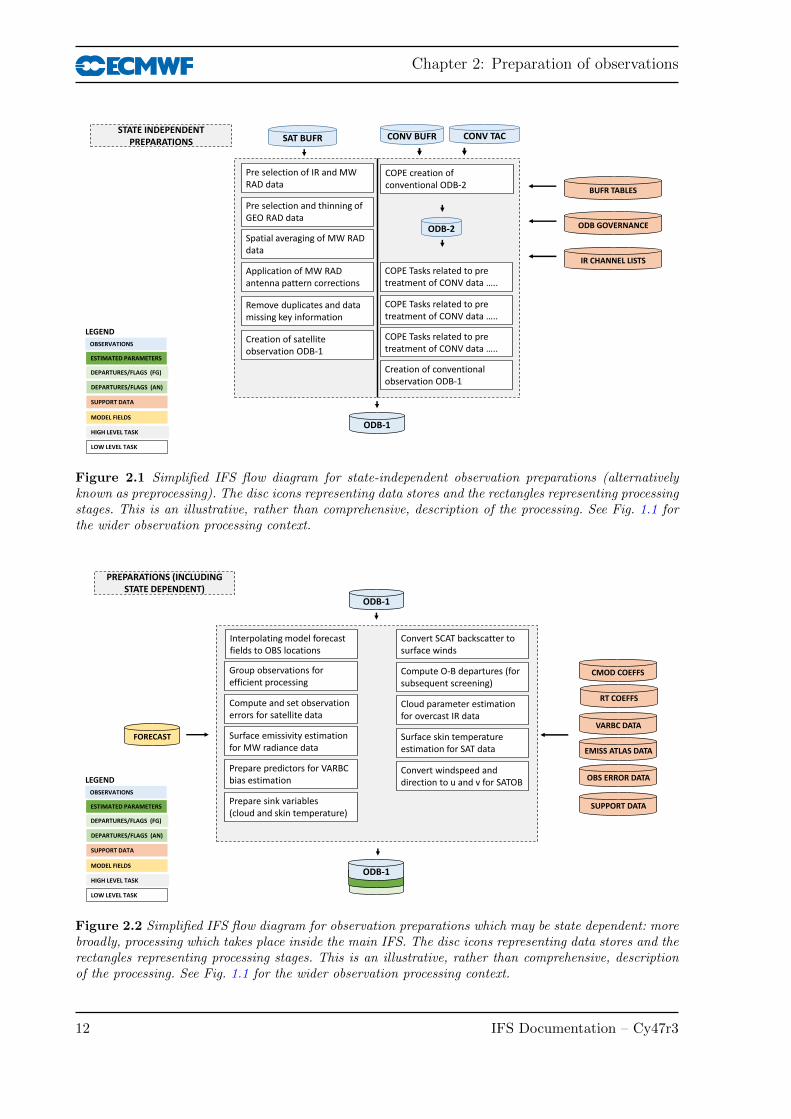
Historically, the upstream observation pre-processing (described here as ‘state-independent preparations’) havenot been part of the IFS documentation. The aim is to bring this more fully into the documentation, but becausethese tasks are in the process of re-factoring under COPE, they will not be covered in great detail. Fig. 2.1illustrates these tasks but is far from comprehensive.
Figure 2.2 summarises broadly the preparations that take place inside the IFS and are mostly ‘state-dependent’.However, viewing the processing in this way is not always helpful. For example, variable conversions, such asfrom wind-speed and direction to horizontal wind components, take place in COPE (in prescreening) forconventional data but in the IFS for satellite-derived AMVs. This chapter is hence mostly structured by thescientific procedure (e.g. parameter conversions, prior retrievals, observation error) rather than the technicallocation in which the science is achieved.
IFS Documentation – Cy47r3 11
Chapter 2: Preparation of observations
SAT BUFR
ODB-1
CONV BUFR CONV TAC
ODB GOVERNANCE
LEGEND
OBSERVATIONS
DEPARTURES/FLAGS (FG)
MODEL FIELDS
SUPPORT DATA
ESTIMATED PARAMETERS
HIGH LEVEL TASK
LOW LEVEL TASK
DEPARTURES/FLAGS (AN)
STATE INDEPENDENT PREPARATIONS
ODB-2
Pre selection of IR and MW RAD data
Pre selection and thinning of GEO RAD data
Spatial averaging of MW RAD data
Application of MW RAD antenna pattern corrections
Remove duplicates and data missing key information
Creation of satellite observation ODB-1
Creation of conventional observation ODB-1
COPE Tasks related to pre treatment of CONV data …..
COPE Tasks related to pre treatment of CONV data …..
COPE Tasks related to pre treatment of CONV data …..
COPE creation of conventional ODB-2
IR CHANNEL LISTS
BUFR TABLES
Figure 2.1 Simplified IFS flow diagram for state-independent observation preparations (alternativelyknown as preprocessing). The disc icons representing data stores and the rectangles representing processingstages. This is an illustrative, rather than comprehensive, description of the processing. See Fig. 1.1 forthe wider observation processing context.
LEGEND
OBSERVATIONS
DEPARTURES/FLAGS (FG)
MODEL FIELDS
SUPPORT DATA
ESTIMATED PARAMETERS
HIGH LEVEL TASK
LOW LEVEL TASK
DEPARTURES/FLAGS (AN)
ODB-1
PREPARATIONS (INCLUDING STATE DEPENDENT)
EMISS ATLAS DATA
Interpolating model forecast fields to OBS locations
Compute and set observation errors for satellite data
Convert SCAT backscatter to surface winds
Compute O-B departures (for subsequent screening)
OBS ERROR DATA
SUPPORT DATA
VARBC DATA
RT COEFFS
Surface emissivity estimation for MW radiance data
Prepare predictors for VARBC bias estimation
Cloud parameter estimation for overcast IR data
Surface skin temperature estimation for SAT data
CMOD COEFFS
ODB-1
FORECAST
Prepare sink variables(cloud and skin temperature)
Group observations for efficient processing
Convert windspeed and direction to u and v for SATOB
Figure 2.2 Simplified IFS flow diagram for observation preparations which may be state dependent: morebroadly, processing which takes place inside the main IFS. The disc icons representing data stores and therectangles representing processing stages. This is an illustrative, rather than comprehensive, descriptionof the processing. See Fig. 1.1 for the wider observation processing context.
12 IFS Documentation – Cy47r3
Part I: Observations
2.2 NON-COPE STATE-INDEPENDENT PREPARATIONS(PREPROCESSING)
Processing external to COPE still accounts for the majority of data going into the IFS. All satellite data goesthrough the long-established path of BUFR preprocessing (the PREPARE OBS tasks) and BUFR to ODB-2conversion (the BUFR2ODB tasks). In this area, data undergo some rudimentary quality controls, e.g. a checkfor the observation format and position, and for the climatological limits. These jobs are multi-tasked runningin parallel on multiple nodes. Several or all observation types can run synchronously.
2.2.1 Clear-sky satellite radiances
Radiance observations undergo a pre-screening process before being loaded into the ODB for input to the mainIFS screening. Firstly, this is used to reduce the data volume and thus the computational burden of the mainscreening. Secondly, this rejects observations that fail to contain crucial header information and/or the correctnumber of channels that could potentially cause a computational run-time failure in the main screening.Observations in BUFR are decoded and checked inside SCREEN 1C where, additionally, data measured atparticular scan lines and or scan positions may be removed to reduce the data volume (by setting LINE THIN,FOV THIN in the calling script PRE 1CRAD). Observations which survive the checking and thinning processare then re-encoded in BUFR and supplied to the ODB loader. A key consideration for rejecting data in thepre-screening is that removed observations will NOT be passed through the IFS screening and thus will NOTaccrue feedback quality information. Currently all pre-screening tasks are scalar (i.e. not parallel). However,for IASI (by far the largest data volume) the process is effectively parallelized by splitting the input BUFR fileand launching multiple scalar tasks simultaneously.
2.2.2 All-sky microwave radiances
Observations are received in BUFR format and are pre-processed by SCRIPTS/GEN/premwimg for conical-scanning imagers and SCRIPTS/GEN/pre1crad* for sounders. Observations part of the all-sky path are givencodetype 215 (see ODB/CMA2ODB/buf2cmat new).
For imagers, SATRAD/PROGRAMS/bufr grid screen is called to do superobbing. Observations are put onto aGaussian grid corresponding to T255 resolution, but with every second point removed to reduce data volumes.Observations within 60 k of the grid point centres are averaged together to form a superob. This brings therelatively high observation resolution of microwave imagers (up to 10 km) down to roughly the scale of cloudsin the IFS model. The superobbing is done by computing the numerical mean of all BUFR fields, exceptlongitude and latitude, which are taken to be those of the grid-point, and the observation time, which comesfrom the last observation meaned. This program also allows a further thinning of the data by keeping onlyobservations associated with grid points at every nth longitude and mth latitude.
For sounders, there is data thinning but no superobbing. Thinning is done after any antenna pattern correctionsare applied, performed in one hour time slots. AMSU-A is a special case, with thinning performed at T159resolution and in 30 minute time slots considering all AMSU-A sensors together. For humidity sounders thinningis done on a T255 resolution grid, retaining every other point.
2.2.3 Ground-based radar precipitation composites
Prior to their assimilation, the original hourly 4-km NCEP Stage IV surface precipitation composites (basedon NEXRAD ground-based radars and (some) rain gauges over the United States; Lopez, 2011) are averagedover the model grid at trajectory resolution to reduce possible representativeness issues. In addition, onlyobservations that are located east of 105W are selected. This is to avoid the likely degradation of ground-radar-based measurements over the Rocky Mountains due to beam blocking, precipitation enhancement orthe need for a proper correction of vertical profiles of reflectivity at higher radar beam angles. For similarreasons, observations located over high (zorog > 1500 m) or rugged terrain (σorog > 100 m) are rejected. Theobservations are then accumulated over the period NPRACCL, currently set to 21600 seconds in namelistNAEPHY. All this pre-screening is performed by routine BUFR SCREEN NEXRAD. Pre-processed observationsare then converted to log(RR[mm/h]+1) space in routine B2O CONVERT RAIN RATES.
IFS Documentation – Cy47r3 13

Chapter 2: Preparation of observations
2.3 CONTINUOUS OBSERVATION PROCESSING ENVIRONMENT(COPE)
Preparation of conventional in-situ observations is now handled in the COPE environment, prior to the IFS.
The main objective of COPE project has been to consolidate various observation processing tasks that are eithercarried out in IFS screening, BUFR2ODB conversion or in preobs tasks, into a unified modular framework.The first phase of the project was focused on tasks that do not require model information and thus canbe externalized from IFS. Decoupling observation pre-processing from the actual assimilation run has manybenefits. Perhaps the most important being to free computational resources in time critical path and to increaseresilience against anomalies in observing systems.
So far, only conventional in-situ observation pre-processing has been been fully externalized from IFS, replacingthe functionality of MKCMARPL. To activate COPE framework, one needs to set LCOPE option to truein PrepIFS (this is default since 40r3). Activating COPE will automatically disable MKCMARPL workersubroutines for all conventional observations (e.g. AIREPIN, METARIN, etc.). This is done in ifstraj scriptusing LMKCMARPL logical array in NAMOBS namelist to deactivate processing for selected observation types.
More information on the transition from MKCMARPL to COPE can be found in Chapter 5. COPE now handlesconventional, in-situ data in configuration files and new COPE routines, e.g:
• airep.json• dribu.json• temp.json• pilot.json• pgps.json• synop.json• ship.json• awp.json• ewp.json• DateTimeValidator, LocationValidator• error statistics.csv• PrescribedErrorAssigner• FinalErrorAssigner• SpecificHumidityAssigner• InstrumentTypeAssigner• HeightToPressureConverter• RadiosondeBiasCorrector
The JSON configuration files describe processing pipeline for the given observation type in declarative way.This allows to modify or even construct new pipelines at runtime, reusing existing filters, without having torecompile the source. Conceptually, every pipeline is composed of a chain of filters that are sequentially appliedon each observation report. All JSON configuration files can be found in the standard IFS scripts directory.
Since COPE is a collaborative project involving several external partners, its source code is managed undercommon Git repository: https://software.ecmwf.int/stash/projects/COPE/repos/cope.
For SYNOP, SHIP and BUOY reports the usual humidity variable reported is dewpoint temperature and formany years this was the only one extracted. However some (particularly in cold regions) report relative humidityand from 47R1 there is an option (B2O EXTRACT RH2M, default false) to extract this and another option(COPE OVERRIDE RH2M) which determines which is used if both are reported.
2.4 VARIABLE CONVERSIONS INCLUDING RETRIEVALS
Most observations are used in their original form as this is usually the most optimal use of the data. However,some are transformed, either with a change of variable, but also there may be a retrieval from satellite data ifthey are independent from the background model fields. The original variables may be kept with the derivedones so that first guess departures can be assigned for both.
14 IFS Documentation – Cy47r3

Part I: Observations
2.4.1 Conventional observations:
Variables which are transformed for further use by the analysis are as follows.
(i) Wind direction (DDD) and force (FFF) are transformed into wind components (u and v) for SYNOP,AIREP, SATOB, DRIBU, TEMP and PILOT observations.
(ii) Temperature (T) and dew point (Td) are transformed into relative humidity (RH) for SYNOP andTEMP observations, with a further transformation of the RH into specific humidity (Q) for TEMPobservations.
The wind components are worked out as
u=−FFF sin
(DDD
π
180
)v =−FFF cos
(DDD
π
180
)
The RH is derived using
RH =F (Td)
F (T )
where function F of either T or Td is expressed as
F (T ) = aRdry
Rvapeb
T−T0T−c
where T0 = 273.16 K, a= 611.21, b= 17.502, c= 32.19, Rdry = 287.0597 and Rvap = 461.5250 are constants.
The specific humidity Q is worked out by using
Q= RHA
1− RH(
Rvap
Rdry− 1
)A
with function A is expressed as
A=min
[0.5,
F (T )
P
]where P is pressure. Q is assigned in the RH2Q subroutine.
These transformations are (probably) now done in COPE (see Sec. 2.3) except for the SATOB/AMVtransformations, which are still performed underneath the deprecated MKCMARPL (Sec. 5.3)
2.4.2 Scatterometer winds
For ASCAT and possibly some other scatterometers, the retrieval from backscatter to wind is performedinternally to the IFS. This is one of the remaining tasks carried out by the deprecated ‘Make CMA replacement’process (Sec. 5.3).
Dedicated observation operators exist for scatterometer ambiguous surface winds (Stoffelen and Anderson,1997; Isaksen and Janssen, 2004). Backscatters (σ0’s) are transformed into several pairs of ambiguouswind components (u and v); this actually involves a retrieval according to some model function describingthe relationship between winds and σ0’s and requires a fair bit of computational work. The screening ofscatterometer data involves the conversion of the backscatter measurements acquired by the instrument(triplets for ERS and ASCAT and quadruplets for NSCAT and QuikSCAT) into ambiguous u and v windcomponents that will actually be assimilated into the IFS (see Section 3.2.9). The (empirical) relation betweenwind and backscatter is described by a geophysical model function (GMF). Although in principle inverted windcomponents are provided as a level 2 product, at ECMWF the wind inversion is performed in house. In thisway any drifts in backscatter levels can be corrected in a direct manner.
IFS Documentation – Cy47r3 15

Chapter 2: Preparation of observations
Data from the AMI instrument on ERS-2 have been used from June 1996 (with an interruption from January2001 till March 2004), data from the SeaWinds instrument on-board QuikSCAT was used from January 2002until November 2009 (when QuikSCAT failed), and data from ASCAT on MetOp have been assimilatedfrom June 2007 onwards. Data from NSCAT have never been used in an operational setup, although offlineassimilation experiments have been performed. From November 2010 onwards scatterometer data is assimilatedas equivalent-neutral 10-metre wind, rather than (real) 10-metre wind, since the former model winds are closerrelated to scatterometer observations.
(a) Wind retrieval
Since geometry and measurement principle of ERS and ASCAT are alike, data from these instruments isprocessed in a similar way. The procedure for wind inversion closely follows the wind retrieval and ambiguityremoval scheme originally developed for the ERS-1 scatterometer (Stoffelen and Anderson, 1997), thoughthe original geophysical model function CMOD4 has been replaced by CMOD5 (Hersbach et al., 2007) inMarch 2004, by CMOD5.4 in June 2007, and by CMOD5.n (Hersbach, 2010b) in November 2010, after whichscatterometer winds are assimilated as equivalent-neutral wind(Hersbach, 2010a).
For QuikSCAT the task of wind inversion is performed in the pre-screening (PRESCAT). Data are like ERS andASCAT, provided at a resolution of 25 km. Rather than data thinning (see Subsection 4.5.6), for QuikSCAT a50 km product is created which contains information about backscatter from the four underlying original sub-cells. The weight of the scatterometer cost function (defined in routine HJO) of each 50 km wind vector cellis reduced by a factor four, which effectively mimics the assimilation of a 100 km product. It is the re-sampled50 km product that is stored in ODB. Original backscatter observations at 25 km are not available within theassimilation.
In general, the wind retrieval is performed by minimizing the distance between observed backscatter valuesσ0oi and modelled backscatter values σ0
mi given by
D(u) =
n∑i
[(σ0oi)
p − σ0mi(u)
p]2
kp
[∑nj σ0
mj(u)p]2 (2.1)
For ERS and ASCAT data, the sum is over triplets, while for QuikSCAT the sum may extend to 16 values (four25 km sub-cells with each four observations). The quantity p is equal to unity for NSCAT and QuikSCAT.For ERS and ASCAT data, a value of p= 0.625 was introduced because it makes the underlying GMF moreharmonic, which helps to avoid direction-trapping effects (Stoffelen and Anderson, 1997). The noise to signalratio kp provides an estimate for the relative accuracy of the observations.
The simulation of σ0m is for ERS and ASCAT data based on the CMOD5.4 model function. For NSCAT data
the NSCAT-2 GMF has been utilized. For QuikSCAT data, the choice of GMF is handled by a logical switchLQTABLE. By default LQTABLE = .TRUE. and the QSCAT-1 model function is used, otherwise, modelledbackscatter values are based on the NSCAT-2 GMF. The minimization is achieved using a tabular form of theGMF, giving the value of the backscatter coefficient for wind speeds, direction and incidence angles discretizedwith, for ERS and ASCAT data, steps of 0.5 ms−1, 50 and 10, respectively. For NSCAT and QuikSCAT datathe corresponding values are 0.2 ms−1, 2.5 and 1. ERS and ASCAT use the same table, which is read in theinitialisation subroutine INIERSCA. For QuikSCAT, inversion takes place in the QSCAT25TO50KM programin the PRESCAT task.
(b) Quality control
The wind inversion involves some quality control. For ERS (ERS1IF), kp must for each antenna be below 10%,and a missing packet number must be less than 10 to ensure that enough individual backscatter measurementshave been averaged for estimating the value.
For ASCAT (ASCATIF) a in the product provided land fraction must be zero for each backscatter measurement.No restriction on kp is imposed, other than that values should be non missing. It is checked whether two otherprovided quality flags (‘sigma0 usability‘ and ‘kp quality‘) have acceptable values. However, no quality controldecisions are made on these two indicators for the moment, since sofar, they have not been fully calibratedand validated by EUMETSAT.
16 IFS Documentation – Cy47r3

Part I: Observations
For QuikSCAT, from 38 across-track 50 km cells, the outer 4 at either side of the swath are, due to their knownreduced quality rejected. In addition, for QuikSCAT, it is verified whether inverted winds are well-defined, i.e.whether minima D(u) are sufficiently sharp. In practise this is mainly an issue for cells in the central part ofthe swath. Data is rejected when the angle between the most likely solution and its most anti-parallel one isless than 135 (routine SCAQC).
After wind inversion, a further check is done on the backscatter residual associated to the rank-1 solution(also called ‘distance to the cone’). This misfit contains both the effects of instrumental noise and of GMFerrors. Locally, these errors can become large when the measurements are affected by geophysical parametersnot taken into account by the GMF, such as sea-state or intense rainfall. For ERS, a triplet is rejected whenthe cone distance exceeds a threshold of three times its expected value. For QuikSCAT and ASCAT data sucha test is not performed.
In addition to a distance-to-cone test on single observations, a similar test is performed for averages fordata within certain time slots. If these averages exceed certain values, all data within the considered timeslot is suspected to be affected by an instrument anomaly, since geophysical fluctuations are expected to beaveraged out when grouping together large numbers of data points. For ERS and ASCAT, cell-wise averagesare calculated for the default 4D-Var observation time slot (30 minutes) in the IFS routine SCAQC, andits rejection threshold (1.5 times average values) are defined in the IFS routine SUFGLIM. For QuikSCATaverages are considered over six-hourly data files and are evaluated in the pre-screening (DCONE OC), usinga threshold of 1.45 for any of cells between 5 and 34.
(c) Rain contamination
Thanks to the usage of C-band frequency, rain contamination is mild for ERS and ASCAT. For QuikSCATand NSCAT, which operate in Ku band, rain contamination is a serious issue.
For QuikSCAT the check on rain contamination occurs in the pre-screening and is imposed on the original25 km observations. Any 25 km rejected cell is not used in the determination of the 50 km wind product. Whenmore than one 25 km sub-cell is rejected, the entire 50 km product is rejected (decision made in SCAQC).
Since February 2000, the BUFR product provides a rain flag. This flag, which was developed by NASA/JPL,is based on a multidimensional histogram (MUDH) incorporating various quantities that may be used for thedetection of rain (Huddleston and Stiles, 2000). Examples of such parameters are mp rain probability (anempirically determined estimate for the probability of a columnar rain rate larger than 2 m2 hr−1; typicallyvalues larger than 0.1 indicate rain contamination) and nof rain index (a rescaled normalized objective function– values larger than 20 give a proxy for rain). Since at the time of implementation, the quality of the JPL rainflag had not been fully confirmed, an alternative (more aggressive) flag was established in house. Based on astudy in which QuikSCAT winds were compared to collocated ECMWF first guess winds, a quality flag wasintroduced. It is given by
Lrain = nof rain index+ 200 mp rain probability> 30.
Both mp rain probability and nof rain index are provided in the original 25 km BUFR product (for detailssee Leidner et al., 2000). When one of these quantities is missing, the above mentioned condition for theremaining quantity is used.
(d) Bias corrections
For ASCAT and ERS, bias corrections are applied, both in terms of backscatter (before wind inversion) andwind speed (after inversion), particularly to compensate for any change in the instrumental calibration and toensure consistency between the retrieved and model winds. The backscatter and wind-speed bias correctionsare defined by dedicated files read in the initialization subroutine INIERSCA. Files are in principle model-cycle and date dependent. Currently for ERS-2, the appropriate files have no effect (i.e. containing only unitycorrection factors and zeros), since the CMOD5.4 GMF was tuned on ERS-2. For ASCAT, though, the usageof bias corrections is essential, since the backscatter product for this instrument has been calibrated differentlyfrom ERS. The bias correction file for backscatter has been updated every time a change in the calibration ofASCAT was imposed by EUMETSAT.
IFS Documentation – Cy47r3 17

Chapter 2: Preparation of observations
For QuikSCAT data no bias corrections in σ0 space is applied, though, wind-bias corrections are made. Thisalso takes place in the pre-screening. Corrections are performed in three steps. First of all, wind speeds areslightly reduced according to:
v′ = 0.2 + 0.96 v.
Where v is the wind speed as obtained from inversion (2.1) The addition of 0.2 ms−1 is used in theoperational configuration, where scatterometer data is assimilated as equivalent neutral wind. In case thisis not desired (expressed by LSCATT NEUTRAL=false) only the rescaling factor of 0.96 is used. It wasobserved that the residual bias between QuikSCAT winds and ECMWF first guess winds depends on the valueof mp rain probability. The motivation is that, for higher amounts of precipitation, a larger part of the totalbackscatter is induced by rain, leaving a smaller part for the wind signal. The correction applied is
v′′ = v′ − 20⟨ mp rain probability⟩,
where ⟨ ⟩ denotes the average value over the 25 km sub-cells that were taken into account in the inversion(i.e. over rain-free sub-cells). The maximum allowed correction is 2.5 ms−1, which is seldom reached. Finally,for strong winds, QuikSCAT winds were found to be quite higher than their ECMWF first guess counterparts.In order to accommodate this, for winds stronger than 19 ms−1 the following correction is applied:
v′′′ = v′′ − 0.2(v′′ − 19.0).
2.4.3 Adjusted variables
The only observed quantity which is adjusted is the SYNOP’s surface pressure (Ps). This is done by usingpressure tendency (Pt) information, which in turn may be first adjusted. Pt is adjusted only in the case ofSYNOP SHIP data for the ship movement.
The ship movement information is available from input data in terms of ship speed and direction, which arefirst converted into ship movement components Us and Vs. The next step is to find pressure gradient (∂p/∂xand ∂p/∂y) given by
∂p
∂x= C(A1u−A2v)
1
2∂p
∂y=−C(A1u+A2v)
where u and v are observed wind components, and A1 = 0.94 and A2 = 0.34 are the sine and cosine of theangle between the actual and geostrophic winds. C is the Coriolis term multiplied by a drag coefficient (D)so that
C = 2ΩD sin θ
where, θ is the latitude and Ω= 0.7292× 10⁻⁴s−1 is the angular velocity of the earth and D is expressed as
D =GZ
G= 1.25 is an assumed ratio between geostrophic and surface wind over sea and Z = 0.11 kgm−3 is anassumed air density. Now the adjusted pressure tendency (P a
t ) is found as
P at = Pt −
(Us
∂p
∂x+ Vs
∂p
∂y
)Finally, the adjusted surface pressure (P a
s ) is found as
P as = Ps − P a
t ∆t
where, ∆t is a time difference between analysis and observation time. Of course in the case of non-SHIP dataP at ≡ Pt.
These transformations are (probably) now done in COPE (see Sec. 2.3)
18 IFS Documentation – Cy47r3

Part I: Observations
2.4.4 Other conversions
It is worth mentioning the superobbing of all-sky microwave radiances from their raw resolution into a superobmore representative of the cloud and precipitation scales in the forecast model. Currently, all raw observationswithin a 60 km radius of a chosen central point are averaged together. This is done in the BUFR stages ofpre-processing.
2.5 OBSERVATION ERRORS
The diagonal part of the observation errors are written, at some point during the observation processing, intothe ODB column MDBFOE for use by the data assimilation algorithm. However, the source of these errorestimates is varied.
2.5.1 Conventional observations
Three types of observation errors are dealt with at the observation pre-processing level. These steps are nowdone under COPE, external to the IFS. The errors assigned at this stage are persistence observation error,prescribed observation error, and the combination of the two above called the final observation error. Theseare described in the following sections, as well as the additional error inflation for dropsondes, which is donewithin the data assimilation system, as a function of the FG departure.
(a) Persistence observation error
The persistence error is formulated in such a way to reflect its dependence on the following.
(i) Season.(ii) Actual geographical position of an observation.
Seasonal dependency is introduced by identifying three regimes.
(i) Winter hemisphere.(ii) Summer hemisphere.(iii) Tropics.
The positional dependency is then introduced to reflect the dependence on the precise latitude within thesethree regimes.
The persistence error calculation is split into two parts. In the first part the above dependencies are expressedin terms of factors a and b which are defined as
a= sin
(2π
d
365.25+
π
2
)and
b= 1.5 + a
0.5 min
[max(θ, 20)
20
]where d is a day of year and θ is latitude.
The persistence error for time difference between analysis and observation ∆t is then expressed as a functionof b with a further dependence on latitude and a maximum persistence error Emaxpers for 24 hour given by
Epers =Emaxpers
6[1 + 2 sin(|2θ|b∆t)]
where ∆t is expressed as a fraction of a day. The Emaxpers have the values shown in Table 2.1.
Subroutine SUPERERR is used to define all relevant points in order to carry out this calculation, and is calledonly once during the general system initialization. The calculation of the actual persistence error is dealt withby OBSPERR.
IFS Documentation – Cy47r3 19

Chapter 2: Preparation of observations
Table 2.1 Observation persistence errors of maximum 24-hour wind (u, v), height (Z) andtemperature (T ).
Variable (unit) 1000–700 hPa 699–250 hPa 249–0 hPa
u, v (ms−1) 6.4 12.7 19.1Z (m) 48 60 72T (K) 6 7 8
(b) Prescribed observation errors
Prescribed observational errors have been derived by statistical evaluation of the performance of the observingsystems, as components of the assimilation system, over a long period of operational use. Currently,observational errors are defined for each observation type that carries the following quantities.
(i) Wind components.(ii) Height.(iii) Temperature.(iv) Humidity.
As can be seen from the tables of prescribed observation errors, they are defined at standard pressure levelsbut the ones used are interpolated to the observed pressures. The interpolation is such that the observationerror is kept constant below the lowest and above the highest levels, whereas in between it is interpolatedlinearly in ln p. Several subroutines are used for working out the prescribed observation error: SUOBSERR,OBSERR, FIXERR, THIOERR and PWCOERR.
• SUOBSERR defines observation errors for standard pressure levels.• OBSERR and FIXERR calculate the actual values.• THIOERR and PWCOERR are two specialised subroutines to deal with thickness and PWC errors.
Relative humidity observation error RH err is either prescribed or modelled. More will be said about the modelledRH err in Subsection (c). RH err is prescribed only for TEMP and SYNOP data. RH err is preset to 0.17 forTEMP and 0.13 for SYNOP. However, if RH < 0.2 it is increased to 0.23 and to 0.28 if T < 233 K for bothTEMP and SYNOP.
(c) Derived observation errors
Relative humidity observation error, RH err, can also be expressed as function of temperature T so that
RH err =min[0.18,min(0.06,−0.0015T + 0.54)]
This option is currently used for assigning RH err.
Specific humidity observation error, Qerr, is a function of RH , RH err, P, Perr, T and Terr, and formally canbe expressed as
Qerr =Qerr(RH , RH err, P, Perr, T, Terr)
orQerr = RH errF1(RH , P, T )
where function F1 is given by
F1(RH , T, P ) =A[
1− RH(
Rvap
Rdry− 1
)A]2
Subroutine RH2Q is used to evaluate Qerr.
20 IFS Documentation – Cy47r3

Part I: Observations
Surface pressure observation error Pserr is derived by multiplying the height observation error Zerr by aconstant:
Pserr = 1.225 Zerr
However, the Pserr may be reduced if the pressure tendency correction is applied. For non-SHIP data thereduction factor is 4, whereas for SHIP data the reduction factor is either 2 or 4, depending on if the Pt isadjusted for SHIP movement or not.
The thickness observation error (DZ err) is derived from Zerr.
(d) Final (combined) observation error
In addition to the prescribed observation and persistence errors, the so called final observation error is assignedat the COPE stage too. This is simply a combination of observation and persistence errors given by
FOE =√O2
E + P 2E
where FOE, OE and PE are final, prescribed and persistence observation errors, respectively. The subroutineused for this purpose is FINOERR.
(e) Additional error inflation for dropsondes
Dropsonde errors can be inflated further as a function of the first guess departure d, in order to preventproblems in tropical cyclones, where the representation error can be large. This is done in FGWND. A briefsummary is given here; more details can be found in Bonavita et al. (2017). If the ‘final’ observation error isFOE then a new and more final observation error FOE2 is computed by adding a component for representationerror RO:
F 2OE2 = F 2
OE +R2O
where for d2 ≤ F 2OE +B2
O
R2O = 0
and for d2 > F 2OE +B2
O
R2O = d2 − F 2
OE −B2O
Here, BO represents an estimate of background error in observation space.
2.5.2 Satellite observations
(a) Clear-sky radiances
The setup routine DEFRUN sets up initial defaults for clear-sky radiance observation errors, set by sensor andchannel in the variable ROERR RAD1C. Observation errors for 1C radiances are then written to the ODB in acall to RAD1COBE (from HRETR RAD, which runs under the observation operator). However, these valuesare sometimes superseded by situation-dependent error schemes, such as those for the microwave sounders inMW CLEARSKY OBERROR MOD. This is also done within the observation operator code.
For hyperspectral infrared sounder data, DEFRUN first specifies the default observation errors, and thenoverrides these by reading in ASCII files rmtberr airs, rmtberr iasi and rmtberr cris. These files specifyobservation error separately for each channel. For IASI and CrIS, these files also specify the matrices ofobservation error correlations. The observation error specifications for IASI and CrIS are based on backgroundand analysis departure diagnostics as explained in Bormann et al. (2016). Those for AIRS are more conservativeand only loosely based on observation minus background departure data.
(b) All-sky microwave radiances
The observation error is determined using a ‘symmetric’ observation error model which is driven by theobserved and first guess equivalent brightness temperatures. This can only be computed once the observationoperator has been run, so it is computed within the observation operator code under the screening flagLSCREEN=.TRUE. As this is done within the observation operator code, more details are given in Chapter 3.
IFS Documentation – Cy47r3 21

Chapter 2: Preparation of observations
(c) AMVs
Situation-dependent observation errors are computed in AMV OBERR. These are generated within the AMVobservation operator when LSCREEN=.TRUE.
(d) GPSRO
Observation errors are computed in GPSRO OBERROR. These are generated within the observation operatorwhen LSCREEN=.TRUE.
2.5.3 Ground-based radar precipitation composites
In the direct assimilation of NCEP Stage IV surface precipitation composites (using NEXRAD ground-basedradars over the United States), observation error is expressed in log(RR[mm/h]+1) space and is assumed tohave a constant value of 0.2 (resp. 0.1) for rainfall (resp. snowfall). This roughly corresponds to errors of 20%(resp. 10%) in terms of actual precipitation amounts. Practically, these errors are set in routines GBRAD PUTand GBRAD PUT TL.
2.6 BACKGROUND ERROR ESTIMATES FOR SCREENING
All observations are assigned an estimate of the background error in observation space for later use in thebackground quality control (see 4.4.3), and this estimate is stored in the ODB under fg error. This estimateis only used to determine the expected variance of the background departures in the quality control againstthe background, and it is technically separate from the background error used during the assimilation for thecontrol variables to determine the weighting of observations.
The assignment of the fg error is performed in the routine GEFGER, and the method applied depends onthe variable number varno. For the majority of geophysical variables the estimate is based on fields ofsituation-dependent estimates of the background error, calculated from the spread of the EDA. The fieldsare hence consistent with the derivation of the situation-dependent estimate of the background error usedin the assimilation. The fields are available in MARS (scaled ensemble spread, SES), and they are read intovariable RZEGRID in the routine INIFGER. In GEFGER, these fields are horizontally and - if required - verticallyinterpolated to observation locations. This method is applied for all standard geophysical variables (ie, T, q,TCWV, etc), and hence applies, for instance, to conventional observations and AMVs. Scaling of the errorfields by REDNMC used in the assimilation is included. Note, however, that the SES fields are strictly onlyapplicable for the initial time of the assimilation window, and no attempt is made to account for the temporalevolution of the background error pattern.
For observations with more complex observation operators, modifications of the above approach are used,dependent on whether estimates of the EDA spread have previously been calculated for the observed quantity.These result in estimates that may or may not be closely related to values of the actual statistical backgrounderror. This is, for instance, the case for:
Clear-sky radiances: For some clear-sky radiances, background error estimates based on the EDA spread(for a given zenith angle) are available as SES fields, and these are treated similar to the values forstandard geophysical variables. SES fields are available for clear-sky simulations of HIRS, MSU, SSU,AMSU-A, AMSU-B/MHS and SSMI (Bormann and Bonavita, 2013). Where needed, these values areinterpolated to the observation locations. For some other sensors (e.g., geostationary imagers, ATMS,MWTS-2), background error estimates from equivalent channels of the previously named sensors areassigned. While these estimates are not the same as a mapping of the actually used control vectorbackground error into observation space they will capture similar spatial structures.
For hyperspectral infrared instruments (IASI, AIRS, CrIS), the background error estimate is set to 3 K.For most spectral regions this is a severe over-estimation of the uncertainty in the background, and theimplication is that the background error quality control for these instruments is very loose.
All-sky radiances: All-sky radiances do not use situation-dependent estimates from the EDA spread, butrather employ a parametric model, as defined in MWAVE ERROR MODEL.
Bending angles: The background error is set to the same value as the observation error.
22 IFS Documentation – Cy47r3
Part I: Observations
2.7 OTHER PREPARATIONS
2.7.1 Surface emissivity for microwave radiances
(a) Clear-sky microwave
Microwave (EMIS MW N) and infrared (EMIS IR) surface emissivities are set during the screening phase inRAD1CEMIS (called from HRETR RAD) and stored in the ODB for later use by RTTOV. Setting the emissivityto values outside the range of 0 and 1 prompts the calculation of surface emissivity within RTTOV, usingFASTEM (Deblonde and English, 2001) for the microwave and ISEM-6 (Sherlock, 1999) for the infrared. Thisis done for all microwave and infrared radiances over sea.
For microwave radiances over land, several options exist to specify the surface emission, following the methodsdescribed in Karbou et al. (2006). The surface emissivity can be specified through an atlas, or it can bedynamically retrieved from window channel observations and FG estimates of skin temperature and atmosphericprofiles, or the skin temperature can be retrieved given an emissivity atlas value and FG estimates of atmosphericprofiles. Default choices are made by sensor in SUEMIS CONF (including which channel is used for the last twooptions) and can be overwritten through the namelist NAMEMIS CONF or controlled through the PrepIFSswitch AMSU LAND in the Satellites window in the case of AMSU-A/B/MHS. For the two options withdynamic retrieval of emissivity or skin temperature, the required radiative transfer calculations are performedin the routine satrat/rttov/ifs/rttov ec when called from HRETR RAD via RADTR or RADTR ML (see alsonext section). The atlas values and the retrieved emissivities or skin temperatures are written to the ODB, andused as fixed input in subsequent calls to RTTOV. If atlas values are required, these are read in the routineDEFRUN. The default for AMSU-A/B/MHS over land is to use the dynamic retrieval of surface emissivity,using an evolving emissivity atlas to quality-control the retrieved emissivities.
For some microwave sounders such as AMSU-A, a Kalman Filter is used to produce an evolving emissivity atlasfrom past dynamically retrieved emissivity values, as summarised in Krzeminski et al. (2009a) and Bormann(2014). The atlas is updated using the programs EMISKF UPDATE in the satrad project (together with emiskf*and kfgrid* routines that can be found in the emiss directory of the satrad project). The program accesses theODB and reads the required retrieved emissivity values. Only emissivity values that have the datum status flag“use emiskf only” set during the blacklisting are considered. Routine EMISKF INIT specifies the resolutionof the atlas and other configuration settings. Routine EMISKF INIT ATLAS is used to read the atlas values,EMISKF TRAJ to evaluate the new emissivity values against the atlas values, EMISKF PREDICT to predictforward in time the evolution of the errors in the atlas emissivity, and EMISKF UPDATE ATLAS to performthe update of the emissivity parametrization using the Kalman Filter equations, and EMISKF WRITE ATLASto output the updated atlas. To use the atlas with a new sensor/channel, include the new sensor/channelin in the look-up table of known emissivity channels in EMISKF INIT, and provide a new ODBsql view inEMISKF UPDATE. The cycling of the atlas information is done through the files emiskf.cycle* which arestored as tar-ball in ECFS. The routine EMISKF INIT ATLAS is also used to read the atlas under DEFRUNduring the application stage in the screening run. If no atlas is available a “coldstart” is performed, settingthe atlas values and their errors to pre-specified values.
(b) All-sky microwave
A similar framework exists for all-sky microwave radiances, but with the use of a fixed emissivity atlas(TELSEM) instead of an evolving Kalman Filter atlas. A dynamic emissivity retrieval is performed, takinginto account the presence of light cloud and precipitation (Baordo and Geer, 2016). If the retrieval fails, whichgenerally happens if the surface is not fully visible due to heavy cloud or precipitation, then a value is takenfrom the emissivity atlas. This process happens in the observation operator code under MWAVE EMIS, whenLSCREEN=.TRUE.
2.7.2 Cloud affected infrared radiances
For infrared data from HIRS, AIRS and IASI simplified cloud parameters (cloud top pressure and effectivecloud fraction) are estimated for each field of view. Background values are computed during the screening inroutine CLOUD ESTIMATE using a method described in McNally (2009).
IFS Documentation – Cy47r3 23
Chapter 2: Preparation of observations
2.7.3 AMV height reassignment
(a) Legacy height reassignment scheme for diagnostics
A framework exists to perform height reassignment for AMVs when LSCREEN=.TRUE.. This is not usedoperationally. The reassignment is done using the routine AMV REASSIGN, called from HRETR CONV.
(b) Operational reassignment of low-level AMVs
In order to mitigate height assignment problems of AMVs in cases of high wind shear, some AMVs have theirheights reassigned to the model cloud layer average. The scientific motivation for the height reassignmentscheme, and evidence of its beneficial impact on forecast skill, are explained in Lean and Bormann (2021).The height reassignment scheme is used via the LAMV HEIGHT ADJUST=.TRUE. switch.
Model cloud tops and cloud bases are provided by the routine AMV GET MODCLOUD, called fromHRETR CONV. A model level is considered cloudy if its model cloud fraction is above 1%, and the sumof its cloud liquid and ice water content is greater than 10−6 kg/kg. Three consecutive levels must meetthe cloudy criteria for the the routine to record a cloud top and cloud base and therefore for the heightreassignment to be applied to a given AMV.
The reassignment of AMV heights is performed in the routine HRETR CONV. Within this routine furtherconditions are checked beffore the reassignment scheme is applied: the AMV must be between 700 and 900hPa, and must be above the model cloud top. Finally, the scheme is only applied for dates later than 31December 2009, this date cut-off ensures that the height reassignment scheme is only operating when lowlevel clouds are sufficiently represented in the model.
The pre-reassignment AMV height is copied to the variable VERTCO REFERENCE 2 while the height storedin VERTCO REFERENCE 1 is modified. The model u and v wind values at the pre-reassignment height arestored in ODB columns UMOD OLD and VMOD OLD; this is so that O-B statistics can be derived at eitherheight. Optionally, the model cloud-top and cloud-base pressure can be written to the ODB in the CT P andCB P columns.
24 IFS Documentation – Cy47r3

Part I: Observations
Chapter 3
Observation operators
Table of contents3.1 Introduction
3.1.1 Top-level observation operator: HOP
3.1.2 Tangent-linear and adjoint code
3.1.3 Data selection controls: NOTVAR
3.1.4 Test harness
3.1.5 Other tests of the observation operator
3.2 Conventional observation operators
3.2.1 General aspects
3.2.2 Geopotential height
3.2.3 Wind
3.2.4 Humidity
3.2.5 Temperature
3.2.6 Surface observation operators
3.2.7 Atmospheric Motion Vectors
3.2.8 Gas retrievals
3.2.9 Scatterometer winds
3.3 Satellite radiance operators
3.3.1 Common aspects for the setup of nadir radiance assimilation
3.3.2 Clear-sky nadir radiances and overcast infrared nadir radiances
3.3.3 All-sky nadir radiances
3.3.4 Clear-sky limb radiances
3.4 GPS Radio Occultation bending angles
3.5 Ground-based radar precipitation composites
3.6 Atmospheric composition
3.1 INTRODUCTION
The observation operators provide the link between the analysis variables and the observations (Lorenc, 1986;Pailleux, 1990). The observation operator is applied to components of the model state to obtain the modelequivalent of the observation, so that the model and observation can be compared. The operator H signifiesthe ensemble of operators transforming the control variable x into the equivalent of each observed quantity,yo, at observation locations.
From a data assimilation perspective, the job of the observation operator is to interpolate the model state tothe observation location, and then to convert from state variables to observed variables. In the IFS, this job isdivided into two or three parts. The horizontal interpolation to observation locations is handled by the GOMs;this is a complex task requiring multi-process communication to interpolate and to get the model data fromwhichever processors it is located onto the processors where the observation data resides (see part 2). From adataflow point of view, the observation operator is needed in the context of observation preparation, screeningand 4D-Var. Figure 3.1 summarises the operations relevant to observations in 4D-Var. In this observationoperator documentation, we consider a more limited part of the observation operator: the vertical part of theinterpolation (where relevant) and the transformation into observed variables.
IFS Documentation – Cy47r3 25
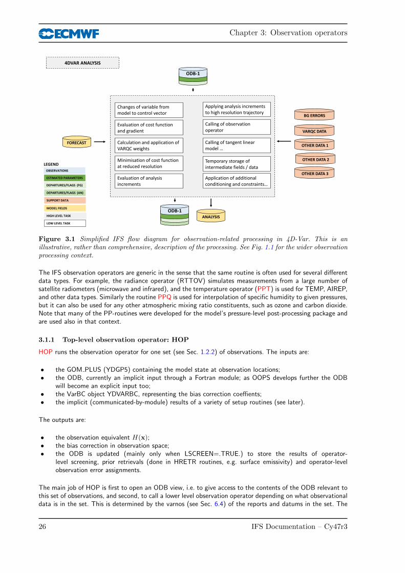
Chapter 3: Observation operators
ODB-1
ODB-1ANALYSIS
4DVAR ANALYSIS
LEGEND
OBSERVATIONS
DEPARTURES/FLAGS (FG)
MODEL FIELDS
SUPPORT DATA
ESTIMATED PARAMETERS
HIGH LEVEL TASK
LOW LEVEL TASK
DEPARTURES/FLAGS (AN)
FORECAST
Changes of variable from model to control vector
Evaluation of cost function and gradient
Calculation and application of VARQC weights
Applying analysis increments to high resolution trajectory
Calling of observation operator
Calling of tangent linear model …
OTHER DATA 1
VARQC DATA
BG ERRORS
Minimisation of cost function at reduced resolution
Evaluation of analysis increments
Temporary storage of intermediate fields / data
Application of additional conditioning and constraints…
OTHER DATA 2
OTHER DATA 3
Figure 3.1 Simplified IFS flow diagram for observation-related processing in 4D-Var. This is anillustrative, rather than comprehensive, description of the processing. See Fig. 1.1 for the wider observationprocessing context.
The IFS observation operators are generic in the sense that the same routine is often used for several differentdata types. For example, the radiance operator (RTTOV) simulates measurements from a large number ofsatellite radiometers (microwave and infrared), and the temperature operator (PPT) is used for TEMP, AIREP,and other data types. Similarly the routine PPQ is used for interpolation of specific humidity to given pressures,but it can also be used for any other atmospheric mixing ratio constituents, such as ozone and carbon dioxide.Note that many of the PP-routines were developed for the model’s pressure-level post-processing package andare used also in that context.
3.1.1 Top-level observation operator: HOP
HOP runs the observation operator for one set (see Sec. 1.2.2) of observations. The inputs are:
• the GOM PLUS (YDGP5) containing the model state at observation locations;• the ODB, currently an implicit input through a Fortran module; as OOPS develops further the ODB
will become an explicit input too;• the VarBC object YDVARBC, representing the bias correction coeffients;• the implicit (communicated-by-module) results of a variety of setup routines (see later).
The outputs are:
• the observation equivalent H(x);• the bias correction in observation space;• the ODB is updated (mainly only when LSCREEN=.TRUE.) to store the results of operator-
level screening, prior retrievals (done in HRETR routines, e.g. surface emissivity) and operator-levelobservation error assignments.
The main job of HOP is first to open an ODB view, i.e. to give access to the contents of the ODB relevant tothis set of observations, and second, to call a lower level observation operator depending on what observationaldata is in the set. This is determined by the varnos (see Sec. 6.4) of the reports and datums in the set. The
26 IFS Documentation – Cy47r3

Part I: Observations
varno determines what physical observation operator is required, for example radiance simulation using RTTOVor a vertical interpolation of humidity. Because observation sets often contain multiple variables, it is possiblefor more than one physical observation operator to be called for the same set. The main physical operatorsare:
• Conventional observations (OBSOP CONV): this covers surface and upper-air observations, aswell as in-situ data and satellite retrievals that include AMVs and scatterometer winds. What links theseobservations is the observed variables are closely related to the model state, so that the main part ofthe observation operator is usually only a vertical interpolation or integration (for example interpolatingto the vertical level of an aircraft observation, or integrating over many model levels for total or partialcolumn ozone observations). All the necessary conventional operators are handled by ‘PP’ or post-processing routines, and are accessed through the top-level PP interface to the observation operator,PPNEW. Section 3.2 covers these observation operators.
• Nadir radiances (OBSOP RAD): this covers both clear-sky and all-sky radiance observations. At alower level, these use either RTTOV or (for all-sky microwave) RTTOV SCATT. See section 3.3
• Limb radiances (OBSOP LIMB): the 2-dimensional model state and 2-dimensional observationoperator for limb radiances is not handled by RTTOV, so limb radiances need their own operator.This code is dormant and not used operationally. See section 3.3
• GPS bending angles (OBSOP GPSRO): this covers satellite radio-occulation, and it usually requires2-D slice through the model to compute the tangent path through the earth’s atmosphere, including thecomputation of the bending angles. See section 3.4
• GPS path delays (ground-based GPS; OBSOP APDSS): Currently only active at Meteo-France,so not discussed further.
• Ground-based radar observations (OBSOP RADAR): This implements the 1D-Bayesian retrievalof Wattrelot et al. (2014) used at Meteo-France, and not discussed further here.
• Precipitation accumulations, (OBSOP PRECIP ACCUM): This enables the assimilation ofNEXRAD rain radar and rain gauges. The model-equivalent precipitation accumulations are computedinside the model physics and then stored directly to ODB, circumventing the normal process of theobservation operator. The main job of the observation operator under HOP is to extract the pre-computed observation equivalent from the ODB. This approach is DEPRECATED and will becomeimpossible in OOPS.
• Atmospheric composition (OBSOP COMPOSITION): This handles observations mainly used inthe Copernicus atmospheric monitoring service, and it covers retrieved constituent variables as well asaerosol optical depth and some other advanced experimental operators. Composition variables wouldnormally be expected to go through the conventional observation route (OBSOP CONV). However, thecomposition route allows proper treatment of the averaging kernels. A more technical link among thecomposition operators is their use of the ‘GEMS’ input model variables, split into greenhouse gases(GHG), reactive gases (CHEM) and aerosols (AERO). Nevertheless, there is much overlap at a scientificand technical level between the conventional and composition parts of the observation operator, so along-term design goal should be to unify them.
3.1.2 Tangent-linear and adjoint code
In the upper levels of the observation operator, tangent-linear (TL) and adjoint (AD) routines are often mergedwith the direct (i.e. nonlinear) version. The top-level observation operator routine, HOP is one example.Within each of these routines the mutually exclusive logicals LLDIRECT, LLTL and LLAD indicate the modeof operation. TL or adjoint mode is activated by the presence of optional arguments containing the additionaldata structures needed in a TL or adjoint context. Whether present or not, these optional arguments cancascade down the calling tree. For example, the GOM PLUS TL structure (model increment at observationlocations) is an optional argument to HOP, which is then optionally passed down to the lower level operators.
In the lower levels of the code, and particularly those that do extensive numerical computation, the direct, TLand adjoint will usually be three separate routines. Merging the three options together into one routine makessense in areas where little numerical computation is done: in many of the routines that have been merged,90% of code was common across the direct, TL and adjoint. Merging the routines reduces the maintenanceoverhead (preventing changes having to be implemented three times over) and makes it easier to keep the
IFS Documentation – Cy47r3 27

Chapter 3: Observation operators
direct, TL and adjoint routines consistent. For example, if a new feature is added in the direct version, it ismore obvious that the TL and adjoint should be updated to reflect this.
Where direct and TL or adjoint variables are present in the same routine, the usual IFS naming conventionapplies:
• VARIABLE5 is the nonlinear (direct) variable;• VARIABLE is the TL or adjoint variable, with its meaning depending on the context (e.g. LLTL or
LLAD);
3.1.3 Data selection controls: NOTVAR
Most data selection criteria are kept in the blacklist or are performed in observation operator code underthe LSCREEN=.TRUE. switch. (see later). However, classes of data can also be switched on and off inthe observation operator using the NOTVAR array in NAMJO. The second dimension in this array is theobservation type. The first dimension is the variable number (varno, see later). The elements of the NOTVARarray can take either of two values: 0, means that the data will be used; −1, means that it won’t. NOTVARis only intended for operational emergencies or debugging, as uniquely it can stop some observations goingthrough the observation operators. The blacklist only stops observations going into the 4D-Var minimisation.If an observation is crashing the observation operator in the screening trajectory, NOTVAR is a temporarysolution; later the code should be re-written to prevent the crash, or the data should be blacklisted in theusual way.
3.1.4 Test harness
The test harness for HOP, HOP DRIVER, is a program that can be run independently of the IFS with suitableinput files:
• GOM PLUS DUMP files containing the model state at observation locations;• ODB-1 files (ECMA and CCMA) containing the ODB;• VARBC.cycle file containing the VarBC coefficients;• HOP RESULTS files containing reference HOP output, for comparison;• All the data files required to run the observation operator, such as RTTOV coefficient files, channel
mappings etc.
To produce these files it is necessary to run the IFS with LHOP RESULTS=true andLGOM PLUS DUMP=true in the TESTVAR namelist. Also it is necessary to restrict the amount ofobservational data to make it feasible to run the test harness interactively on a single node. Further detailscan be found in the test harness README.run file.
In direct mode the test harness runs the observation operator and computes the VarBC bias correction; theseare compared to the reference output and should be bit-identical between offline and online runs of the samecode. In TL and adjoint mode the TL-adjoint consistency test is run, along with a comparison of the TL resultswith reference results from a run of the IFS. There is not yet the facility to test VarBC TL or adjoint or theauxiliary control variables like the skin-temperature sink variable.
3.1.5 Other tests of the observation operator
The adjoint test of the whole 4D-Var operator chain (change of variable, forecast model, interpolation,observation operator) can be activated with NTESTVAR = 1 and LADTEST = .TRUE. There are actuallytwo tests of adjoint triggered here; the relevant one for observations is coded under ADJOTEST. The resultsof this test are printed to the logfiles after ‘Adjoint test obs. operator 1.234567890123456789’.
An adjoint test of the RTTOV clear-sky observation operator, on a per-set basis, can be activated withNTESTVAR = 1 and LRTTOV ADTEST = .TRUE.
28 IFS Documentation – Cy47r3

Part I: Observations
3.2 CONVENTIONAL OBSERVATION OPERATORS
3.2.1 General aspects
This section describes the great variety of observation operators handled by OBSOP CONV and underneath,PPNEW, which is a wrapper for all the PP routines.
The vertical operations depend on the variable. The vertical interpolation is linear in pressure for temperature(PPT) and specific humidity (PPQ), and it is linear in the logarithm of pressure for wind (PPUV). Thevertical interpolation of geopotential (PPGEOP) is similar to wind (in order to preserve geostrophy) andis performed in terms of departures from the ICAO standard atmosphere for increased accuracy (Simmonsand Chen, 1991. The current geopotential vertical interpolation together with the temperature verticalinterpolation are not exactly consistent with hydrostatism. A new consistent and accurate vertical interpolationhas been devised by Meteo-France, which may be important for intensive use of temperature information.The new routines have been tested by ECMWF and as the results were not unambiguously positive thenew routines have not yet been adopted – and they are not described in this documentation. In themeantime, the old routines are still used (switch LOLDPP = .TRUE. in namct0), under the names PPT OLD,PPGEOP OLD and PPUV OLD, with tangent linear PPTTL OLD, PPGEOPTL OLD and PPUVTL OLD andadjoint PPTAD OLD, PPGEOPAD OLD and PPUVAD OLD.
The vertical interpolation operators for SYNOP 10-metre wind (PPUV10M) and 2-metre temperature(PPT2M) match an earlier version of the model’s surface layer parametrization. The vertical gradients ofthe model variables vary strongly in the lowest part of the boundary layer, where flow changes are inducedon very short time and space scales, due to physical factors such as turbulence and terrain characteristics.The vertical interpolation operator for those data takes this into account following Monin–Obukhov similaritytheory. Results using such operators, which follow Geleyn (1988) have been presented by Cardinali et al.(1994). It was found that 2-metre temperature data could not be satisfactorily used in the absence of surfaceskin temperature as part of the control variable, as unrealistic analysis increments appeared in the near-surfacetemperature gradients. The Monin–Obukhov based observation operator for 10-metre wind, on the other hand,is used for all surface winds (SYNOP, DRIBU, TEMP, PILOT and SCAT), where interpolation is not confinedto only 10 m, but is performed to the actual observation height (in practice ranging from 4 to 10 m).
Relative humidity is assumed constant in the lowest model layer to evaluate its 2-metre value (PPRH2M),see Subsection (e). Model equivalents of total column water vapour data are obtained by vertical integrationof q (in GPPWC and PPPWC). The routine PPPWC is also used for vertical integration of GEMS/MACCtrace gasses. Observation operators exist for precipitable water content (also using PPPWC) and thicknesses(PPGEOP).
The details regarding observation operators for conventional data can be found in Vasiljevic et al.(1992), Courtier et al. (1998), and in the following sections.
3.2.2 Geopotential height
The geopotential at a given pressure p is computed by integrating the hydrostatic equation analytically using theICAO temperature profile and vertically interpolating ∆ϕ, the difference between the model level geopotentialand the ICAO geopotential (Simmons and Chen, 1991). The ICAO temperature profile is defined as
TICAO = T0 −Λ
gϕICAO (3.1)
where T0 is 288 K, ϕICAO is the geopotential above 1013.25 hPa and Λ is 0.0065 K m−1 in the ICAOtroposphere and 0 in the ICAO stratosphere (the routine PPSTA). The ICAO tropopause is defined by thelevel where the ICAO temperature has reached 216.5 K (SUSTA). Using this temperature profile and integratingthe hydrostatic equation provides TICAO and the geopotential ϕICAO as a function of pressure (PPSTA). Wemay then evaluate the geopotential ϕ(p) at any pressure p following
ϕ(p)− ϕsurf = ϕICAO(p)− ϕICAO(psurf) + ∆ϕ (3.2)
where psurf is the model surface pressure and ϕsurf , the model orography. ∆ϕ is obtained by verticalinterpolation from the full model level values ∆ϕk. The interpolation is linear in ln(p) up to the second
IFS Documentation – Cy47r3 29

Chapter 3: Observation operators
model level (PPINTP) and quadratic in ln(p) for levels above it (PPITPQ, see below). Following Simmonsand Burridge (1981) the full model level values are obtained by integrating the discretized hydrostatic equationusing the routine GPGEO of the forecast model to give
∆ϕk =
k+1∑j=L
Rdry(Tvj− TICAOj
) ln
(pj+1/2
pj−1/2
)+ αkRdry(Tvk
− TICAOk) (3.3)
with
αk = 1−pk−1/2
pk+1/2 − pk−1/2ln
(pk+1/2
pk−1/2
)for k > 1 and α1 = ln(2).
(a) Quadratic vertical interpolation near the top of the model
Above the second full level of the model, the linear interpolation (PPINTP) is replaced by a quadraticinterpolation in ln p, performed in the routine PPITPQ using
z(ln p) = a+ b(ln p) + c(ln p)2 (3.4)
where a, b and c are constants determined so that the above equation fits the heights at the top levels (k = 1, 2and 3). The interpolation formula is
ϕ(ln p) = z2 +(z2 − z1)(ln p− ln p2)(ln p− ln p3)
(ln p2 − ln p1)(ln p1 − ln p3)− (z2 − z3)(ln p− ln p1)(ln p− ln p2)
(ln p2 − ln p3)(ln p1 − ln p3)(3.5)
where 1,2 and 3 refer to levels k = 1, 2 and 3, respectively.
(b) Below the model’s orography
The extrapolation of the geopotential below the model’s orography is carried out as follows: Find T ∗ (surfacetemperature) by assuming a constant lapse rate Λ, from the model level above the lowest model level (subscriptl − 1), see the routine CTSTAR, using
T ∗ = Tl−1 + ΛRdry
gTl−1 ln
psurfpl−1
(3.6)
T ∗ =T ∗ +max[Ty,min(Tx, T
∗)]2
(3.7)
Find the temperature at mean sea level, T0 (also in CTSTAR) from
T0 = T ∗ + Λϕsurf
g(3.8)
T0 =min[T0,max(Tx, T∗)] (3.9)
where Tx is 290.5 K and Ty is 255 K. The geopotential under the model’s orography is (in PPGEOP) calculatedas
ϕ= ϕsurf −RdryT
∗
γ
[(p
psurf
)γ− 1
](3.10)
where γ =Rdry
ϕsurf(T0 − Tsurf).
3.2.3 Wind
In PPUV a linear interpolation in ln p (PPINTP) is used to interpolate u and v to the observed pressure levelsup to the second full model level, above which a quadratic interpolation is used (PPITPQ. Below the lowestmodel level wind components are assumed to be constant and equal to the values of the lowest model level.
30 IFS Documentation – Cy47r3

Part I: Observations
3.2.4 Humidity
Specific humidity q, relative humidity U and precipitable water content PWC are linearly interpolated in p,in PPQ, PPRH and PPPWC, respectively. Upper air relative humidity data are normally not used, but couldbe used, if required. The use of surface relative humidity data is described in Subsection (e).
(a) Saturation vapour pressure
The saturation vapour pressure esat(T ) is calculated using Tetens’s formula given by
esat(T ) = a1 expa3
(T−T3T−a4
)(3.11)
using FOEEWM (mixed phases, water and ice) in the model and FOEEWMO (water only) for observations. Theuse of water-phase only is in accordance with the WMO rules for radiosonde and SYNOP reporting practices.Note that these statement functions compute (Rdry/Rvap)esat(T ), with the parameters set according to Buck(1981) and the AERKi formula of Alduchov and Eskridge (1996), i.e. a1 = 611.21 hPa, a3 = 17.502 anda4 = 32.19 K over water, and for FOEEWM a3 = 22.587 and a4 =−0.7 K over ice, with T3 = 273.16 K.Furthermore in FOEEWM the saturation value over water is taken for temperatures above 0C and the valueover ice is taken for temperatures below −23C. For intermediate temperatures the saturation vapour pressureis computed as a combination of the values over water esat(water) and esat(ice) according to the formula
esat(T ) = esat(ice)(T ) + [esat(water)(T )− esat(ice)(T )]
(T − Ti
T3 − Ti
)2(3.12)
with T3 − Ti = 23 K.
(b) Relative humidity
In GPRH relative humidity U is computed from
U =pq
Rvap
Rdry[1 +
(Rvap
Rdry− 1
)q]esat(T )
(3.13)
and then in PPRH interpolated to the required observed pressure levels (using PPINTP). Below the lowestmodel level and above the top of the model is U assumed to be constant. Saturation vapour pressure iscalculated using FOEEWMO if GPRH has been called form the observation operator routines, and usingFOEEWM if called from the model post processing.
(c) Precipitable water
In GPPWC precipitable water is calculated as a vertical summation from the top of the model by
PWC k =1
g
k∑i=1
qi(pi − pi−1) (3.14)
and then in PPPWC interpolated to the required observed pressure levels (using PPINTP). PWC is assumedto be zero above the top of the model. Below the model’s orography PWC is extrapolated assuming a constantq = ql.
(d) Specific humidity
Specific humidity q is in PPQ interpolated to the required observed pressure levels (using PPINTP). Belowthe lowest model level and above the top of the model is q assumed to be constant and equal to ql and q1,respectively.
3.2.5 Temperature
Temperature is interpolated linearly in pressure (PPINTP), in the routine PPT. Above the highest model levelthe temperature is kept constant and equal to the value of the highest model level. Between the lowest model
IFS Documentation – Cy47r3 31

Chapter 3: Observation operators
level and the model’s surface the temperature is interpolated linearly, using
T =(psurf − p)Tl + (p− pl)T
∗
psurf − pl(3.15)
Below the lowest model level the temperature is extrapolated by
T = T ∗[1 + α ln
p
psurf+
1
2
(α ln
p
psurf
)2+
1
6
(α ln
p
psurf
)3](3.16)
with α= ΛRdry/g, for ϕsat/g < 2000 m, but α is modified for high orography to α=Rdry(T′0 − T ∗)/ϕsurf ,
whereT ′0 =min(T0, 298) (3.17)
for ϕsurf/g > 2500 m, and
T ′0 = 0.002[(2500− ϕsurf/g)T0 + (ϕsurf/g − 2000) min(T0, 298)] (3.18)
for 2000< ϕsurf/g < 2500m. If T ′0 < T ∗ then α is reset to zero. The two temperatures T ∗ and T0 are computed
using (3.6) to (3.9).
3.2.6 Surface observation operators
Preparations for the vertical interpolation of surface data are done in during the creation of the GOM PLUS.Here dry static energy (SURBOUND), Richardson number, drag coefficients and stability functions (EXCHCO)are computed. For scatterometer data, information on equivalent neutral 10-metre wind is directly fetchedfrom the physics package (via the GOM arrays) which is preprocessed in routine EXCHCO VDF. The actualvertical interpolation is performed in PPOBSAS, which embraces routines for 10-metre vector-wind components(PPUV10M), 2-metre temperature (PPT2M) and 2-metre relative humidity (PPRH2M).
The routines mentioned above for 2-metre temperature and humidity and 10-m wind were superceded someyears ago by SPPCFL, documented in Chapter 3.10 of Part 4 of the IFS documentation. At CY47R1 an optionto use the newer routines in the surface observation operators was added (this is L SCREEN LEVEL OBSOPdefault false). The 2-metre temperature (or humidity) is interpolated between the value at the lowestmodel level and the surface value (and the fact that the 4D-Var control variable does not contain surfacetemperature may cause a problem). Note that this alternative does not use PPNEW but that values are setin OBSOP CONV. Also note that 2-metre relative humidity (which still uses the old observation operator)is replaced by 2-metre specific humidity as the assimilated variable. There is a technical issue in that modelequivalents for the first time step (15 minutes) are not available so for now these values are blacklisted if thenew option is used - the number of stations affected is quite small since most report ”on the hour”. There isanother new namelist variable (4DLAPSET2, default 0.0065 K/m) which is the lapse rate used in 4D-Var forT2m to adjust for the difference between station height and model orography (if L SCREEN LEVEL OBSOPis true). Similar or identical adjustments are used in other NWP systems (eg Ingleby (2015)) and also in theverification against SYNOPs at ECMWF.
(a) Vertical interpolation
For wind and temperature an analytical technique (Geleyn, 1988) is used to interpolate values between thelowest model level and the surface. It is based on Monin–Obukhov theory in which simplified versions ofstability functions ϕM and ϕH are used. The following equations are to be integrated:
∂u
∂z=
u∗
κ(z + z0)ϕM
(z + z0L
), (3.19)
∂s
∂z=
s∗κ(z + z0)
ϕH
(z + z0L
), (3.20)
L=cpg
T
κ
u2∗
s∗, (3.21)
32 IFS Documentation – Cy47r3
Part I: Observations
were u, s are wind and energy variables, u∗, s∗ are friction values, u∗ = |u∗|, and κ= 0.4 is von Karman’sconstant. Note that u denotes the vector wind relative to a surface current u0,
u= ua − u0, (3.22)
with ua the wind in the absolute (model) frame. In default configuration (global variable LECURR is false)surface current is zero, in which case the distinction between absolute and relative wind is irrelevant.
The temperature is linked to the dry static energy s by
s= cpT + ϕ (3.23)
cp = cpdry
[1 +
(cpvap
cpdry
− 1
)q
]. (3.24)
The neutral surface exchange coefficient at the height z is defined as
CN =
[κ
ln(
z+z0z0
)]2, (3.25)
where z0 is the surface roughness length. Drag and heat coefficients are defined as
CM =u2∗
[u(z)]2, (3.26)
CH =u∗s∗
u(z)[s(z)− s], (3.27)
where u(z) = |u(z)| and s is the dry static energy at the surface. Details on the estimation of the roughnesslength and transfer coefficients can be found in Subsection (c).
For convenience the following quantities are introduced:
BN =κ√CN
, BM =κ√CM
, BH =κ√CM
CH. (3.28)
For stable conditions the (simplified) stability function is assumed
ϕM/H = 1 + βM/Hz
L, (3.29)
and integration of (3.19) and (3.20) from 0 to z1 (the lowest model level) leads to values for relative windu(z) and static energy s(z) at observation height z:
u(z) =u(z1)
BM
[ln
(1 +
z
z1(eBN − 1)
)− z
z1(BN −BM)
], (3.30)
s(z) = s+s(z1)− s
BH
[ln
(1 +
z
z1(eBN − 1)
)− z
z1(BN −BH)
]. (3.31)
In unstable conditions the stability function is chosen as
ϕM/H =
(1− βM/H
z
L
)−1
(3.32)
and the vertical profiles for relative wind and dry static energy are then given by
u(z) =u(z1)
BM
[ln
(1 +
z
z1(eBN − 1)
)− ln
(1 +
z
z1(eBN−BM − 1)
)], (3.33)
s(z) = s+s(z1)− s
BH
[ln
(1 +
z
z1(eBN − 1)
)− ln
(1 +
z
z1(eBN−BH − 1)
)]. (3.34)
IFS Documentation – Cy47r3 33

Chapter 3: Observation operators
In case the influence of stability is neglected, the following equivalent-neutral wind profile un(z) is obtained:
un(z) =u(z1)
BMln
(1 +
z
z1(eBN − 1)
). (3.35)
For wind, the relevant routine PPUV10M embodies this method of Geleyn (1988) to estimate vectorwind components at observation height z from provided lowest model level wind u(z1) = ua(z1)− u0. Forscatterometer data, by default, relative wind (3.30), (3.33) is returned, while for all other data the wind in theabsolute frame is evaluated:
ua = u+ u0. (3.36)
For scatterometer data, by default equivalent-neutral wind (3.35) is returned. In case non-neutral wind is tobe assimilated (operational before November 2010), a variable LSCATT NEUTRAL is to be set to false.
The temperature at observation height z = 2 m is evaluated in PPT2M. It is obtained from s as
T (z) = s(z)− zg
cp, (3.37)
where s is interpolated according to (3.31) and (3.34).
The vertical interpolation relies on estimates for coefficients BM, BN for wind, and on coefficients BH, BN
and dry static energy at the surface s= s (Tsurf , q = 0). These are provided in the routines EXCHCO,EXCHCO VDF and SURBOUND, and are described in the following two subsections.
(b) Surface values of dry static energy
To determine the dry static energy at the surface we use (3.23) and (3.24) where the humidity at the surfaceis defined by
q = q(z = 0) = h(Csnow, Cliq, Cveg)qsat(Tsurf , psurf) (3.38)
where, according to Blondin (1991), h is given by
h= Csnow + (1− Csnow)[Cliq + (1− Cliq)h] (3.39)
with
h=max
0.5
(1− cos
πϑsoil
ϑcap
),min
(1,
q
qsat(Tsurf , psurf)
)(3.40)
where ϑsoil is the soil moisture content and ϑcap is the soil moisture at field capacity (2/7 in volumetric units).Equation (3.39) assigns a value of 1 to the surface relative humidity over the snow covered and wet fractionof the grid box. The snow-cover fraction Csnow depends on the snow amount Wsnow so that
Csnow =min
(1,
Wsnow
Wsnowcr
)where Wsnowcr = 0.015 m is a critical value. The wet skin fraction Cliq is derived from the skin-reservoir watercontent Wliq by
Cliq =min
(1,
Wliq
Wliqmax
),
whereWliqmax
=Wlayermax(1− Cveg) + CvegAleaf
with Wlayermax= 2× 10⁻⁴ m being the maximum amount of water that can be held on one layer of leaves,
or as a film on bare soil, Aleaf = 4 is the leaf-area index, and Cveg is the vegetation fraction.
34 IFS Documentation – Cy47r3
Part I: Observations
(c) Transfer coefficients
Comparing the (3.19) and (3.20) integrated from zo to z + z0 with (3.25) to (3.27) , CM and CH can beanalytically defined:
1
CM=
1
κ2
[∫∫∫ (z+z0)
z0
ϕM(z′/L)
z′dz′
]2(3.41)
1
CH=
1
κ2
[∫∫∫ (z+z0)
z0
ϕM(z′/L)
z′dz′
∫∫∫ (z+z0)
z0
ϕH(z′/L)
z′dz′
](3.42)
Because of the complicated form of the stability functions, the former integrals have been approximated byanalytical expressions, formally given by (coded in EXCHCO)
CM = CNfM
(Ri ,
z
z0
)CH = CNfH
(Ri ,
z
z0
) (3.43)
where CN is given by (3.25). The bulk Richardson number Ri is defined as
Ri =g∆z∆Tv
cpTv|∆u|2(3.44)
where Tv is the virtual potential temperature. The functions fM and fH correspond to the model instabilityfunctions and have the correct behaviour near neutrality and in the cases of high stability (Louis, 1979; Louiset al., 1982).
(i) Unstable case Ri < 0
fM = 1− 2bRi
1 + 3bcCN
√(1 + z
z0
)(−Ri)
, (3.45)
fH = 1− 3bRi
1 + 3bcCN
√(1 + z
z0
)(−Ri)
, (3.46)
with b= c= 5.(ii) Stable case Ri > 0
fM =1
1 + 2bRi/√(1 + dRi)
, (3.47)
fM =1
1 + 3bRi/√(1 + dRi)
, (3.48)
with d= 5.
(d) Extraction of stability information from the ECMWF surface-layer physics
The estimation of transfer coefficients as described above (Louis, 1979; Louis et al., 1982) does not overlapwell with the stability as evaluated in the full nonlinear surface layer physics parametrization, for two reasons.First, the method of Louis (1979); Louis et al. (1982) does not correspond anymore with the presently usedparametrization. And second, the estimation of the neutral exchange coefficient (3.25) uses (for technicalreasons) a roughness length z0 that is based on climatology, rather than on the actual roughness. Over oceansthis embraces a value of z0 = 1mm , which is typically one order of magnitude too high. The effect on theestimation on 10-metre wind appears to be negligible, however, for 10-metre equivalent neutral wind (used forscatterometer data) and wind at 4 or 5 metre height (typical buoy observation height) a systematic effect canbe observed (Hersbach, 2010a).
IFS Documentation – Cy47r3 35
Chapter 3: Observation operators
As an alternative, the information on stability can be extracted from the 10-metre equivalent neutral windun as evaluated in SPPCFL MOD in the ECMWF surface-layer physics, which is activated by a switchLVDFTRAJ=true. In that case, over the ocean roughness length z0 is estimated from un and the ocean-wave Charnock parameter α, by an approximate solution (Hersbach, 2011) of the following set of implicitequations (coded in Z0SEA):
z0 = αMν
u∗+ α
u2∗g, (3.49)
un =u∗
κlog(1 + z10/z0). (3.50)
Here z10 = 10 m, αM = 0.11, κ= 0.4 is the Von Karman constant, g = 9.80665 ms−2 is the gravitationalacceleration, and ν = 1.5x10⁻⁵m2s−1 the kinematic viscosity.
The coefficient CN is, again evaluated by (3.25), but now using the improved estimate of zo, while coefficientCM for momentum is given by (EXCHCO VDF):
CM =B2M/κ, BM = log(1 + z10/z0)||u(z1)||/un. (3.51)
In the operational configuration this method is only used for the assimilation of scatterometer wind. Forother observables, the method of Louis (1979); Louis et al. (1982) (LVDFTRAJ=false) is used. RoutineEXCHCO VDF does not provide an estimate for the coefficient CH for heat.
(e) Two-metre relative humidity
In GPRH relative humidity is computed according to (3.13). The relative humidity depends on specific humidity,temperature and pressure (q, T and p, respectively) at the lowest model level. It is constant in the surfacemodel layer, see PPRH2M.
3.2.7 Atmospheric Motion Vectors
Groups of AMVs (aka SATOBs) are set up in the routine SUAMV, one group per satellite, computationalmethod, and codetype. The information is stored in the satob group table, residing in the module YOMSATS.
The group table also specifies what type of observation operator is to be used for the particular group (entryobs oper). The default used in operations is to assimilate all AMVs as single-level wind observations (Tomassiniet al., 1998; Bormann et al., 2003), in the same way as conventional data, using the same interpolation routine.Other options are treating AMVs as layer averages, with weights defined, for instance, by a boxcar weightingfunction.
3.2.8 Gas retrievals
Retrievals of atmospheric species such as ozone or water vapour are used in the form of integrated layersbounded by a top and bottom pressure which are given as a part of the observation. The same observationoperator is used as for precipitable water (PPPWC). The same concept is applied to all data, whether it istotal column data (like TOMS and GOME ozone data or MERIS total column water vapour) or data withhigher vertical resolution (like SBUV). For ozone, variational bias correction is implemented (see Part II, classname “to3”, module VARBC TO3). SBUV data is currently used as anchor for the variational bias correctionof ozone and therefore assimilated without bias correction.
3.2.9 Scatterometer winds
For ERS-2 and ASCAT normally two ambiguous pairs of u-component and v-component observations arefound at each SCAT location – with directions approximately 180 degrees apart. QuikSCAT can have 2, 3 or 4ambiguous winds. Up to the first NSCAWSOLMAX (4 by default, adaptable through the namelist NAMSCC)wind solutions are accepted. In case only one ambiguity is found, the report is rejected. If LQSCATT= .TRUE.(the default, modifiable through the namelist NAMJO), the normal quadratic Jo will be used. In this caseonly the SCAT wind nearest to the high resolution background will be used (which is determined in a sectionof HOP). For winds that are not closest to the first guess or analysis, global datum event flag 9, respectively
36 IFS Documentation – Cy47r3

Part I: Observations
10 is set (see Table 6.25). For the latter case datum status is set to rejected as well (Table 6.24). WhenLQSCATT= .FALSE, the two first winds are used and the ambiguity removal takes place implicitly througha special SCAT cost-function (see part II), in HJO (Stoffelen and Anderson, 1997). In that case for QuikSCATthe most likely wind (highest a priori probability) and its most opposing ambiguity are selected.
Routine PPUV10M is like SYNOP, SHIP and DRIBU wind, also used also for SCAT data. Difference is that(in case account is taken for ocean current) the relative wind rather than the absolute wind is returned (notactive in the operational suite, though), and the evaluation of equivalent-neutral wind rather than the real wind(which latter includes for scatterometer data undesired stability effects; operational since November 2011).
3.3 SATELLITE RADIANCE OPERATORS
The majority of satellite data assimilated currently is radiances, all of it going through the top-level observationoperator OBSOP RAD. Radiances, rather than retrieved products, are assimilated directly (Andersson et al.,1994), wherever possible. The current operational configuration uses clear level-1C radiances from a numberof sensors, including ATOVS (McNally et al., 1999), AIRS, IASI, ATMS, as well as geostationary water vapourclear-sky radiances (Munro et al., 2004).
Clear, cloudy and precipitation-affected radiances from microwave imagers, humidity sounders, and temperaturesounders (AMSU-A) are assimilated using an all-sky approach. Hence there are currently two observationoperators active in the IFS to assimilate satellite radiances, one for clear-sky radiances and totally overcastinfrared radiances, and one for all-sky microwave radiances. The observation operators for both routes aredifferent flavours of the RTTOV radiative transfer model (Saunders and Matricardi, 1998; Matricardi et al.,2001), currently using RTTOV version 12.1.
This section also covers the (non-operational) satellite limb radiances that are handled under OBSOP LIMBas they have many commonalities.
3.3.1 Common aspects for the setup of nadir radiance assimilation
The operational radiance assimilation shares the following setup aspects for both radiance assimilation routes.The datasets are distinguished by a satellite ID, a sensor ID, and a codetype. The latter is used to distinguishclear-sky (codetype=210=NGTHRB) or all-sky radiances (codetype=215=NSSMI).
The main set-up routine for radiances is SURAD. It recognises BUFR satellite IDs (call to GETSATID), readsRTTOV coefficient files (call to RTSETUP), and builds a “satellite group table” containing information onwhich satellite groups are present.
(a) Satellite identifiers and sensors
Satellite identifiers are dealt with in the routine GETSATID, called from SURAD. The ODB contains theidentifiers as given in the original BUFR messages. Lists of identifiers for which data exist in any given ODBare prepared in the routine SURAD. The routine GETSATID matches those BUFR satellite identifiers with theplatform and satellite numbers used by the RT-code (e.g. platform 1, satellite 10 for NOAA-10). New satelliteIDs need to be defined in GETSATID, but the id-conversion tables can also be modified through the namelistNAMSATS.
The various types of radiance data in the IFS are also classified by sensor. Each satellite sensor is assigned anumber, defined in the module YOMSATS. The sensor number is used as index to various tables containingobservation errors, BgQC thresholds, VarQC parameters, the Jo-table JOT, etc. See the routine DEFRUN.
(b) Satellite group table
Various satellite-related indices are gathered in the routine SURAD in the FORTRAN90 data structure calledthe ‘satellite group table’, satgrp t (defined in YOMSATS). The table contains elements such as the satellite ID,the sensor ID, the codetype, a sequence number for addressing the transmittance coefficients (rtcoef pos), thenumber of channels, a channel number list, etc. The various satellite-related indices are universally determinedacross all processors. There is one entry in the satellite group table per satellite, sensor, and codetype. A list
IFS Documentation – Cy47r3 37
Chapter 3: Observation operators
of all the satellite groups that were found in the ODBs can be found in the ifstraj output by searching forSATGRP.
(c) Radiative transfer coefficients, pressure levels and validation bounds
Various preparations for RTTOV calculations are set-up in the call to RTSETUP from SURAD. Thisincludes reading of the various coefficient files required by RTTOV. The files can be found under/home/rd/rdx/data/ < cycle > /sat/rttov. There is one file with the prefix rtcoef containing coefficientsfor the general clear-sky radiative transfer for each instrument and satellite, and files with prefix sccldcoefused for a parametrization of cloud scattering effects for some infrared sensors. Both types of files are read viaa call to RTTVI (in the satrad library) which also communicates other settings from the RTTOV code in thesatrad library to the IFS side. Only the files that are required are read, i.e. only the files for which observationsare present (for the clear-sky coefficients) or for which data is present and the calculation of cloudy radiances isrequested through switching the flags LCLD RTCALC SCREEN or LCLD RTCALC ASSIM on in the moduleSATS MIX for the respective sensor. A third type of RTTOV coefficient files (prefix mietable ) is requiredfor RTTOV SCATT computations in the all-sky system (see 3.3.3), read via a call to MWAVE SETUP underRTSETUP.
The transmittance coefficient file for different sensors can use any number of fixed pressure levels, and thenumber can be different for different sensors. However, interpolation to RTTOV pressure levels is performedinside RTTOV - see 3.3.2 - so the IFS does not need to know about that.
3.3.2 Clear-sky nadir radiances and overcast infrared nadir radiances
(a) Bias correction
The bias correction is performed through variational bias correction, see part II. The VarBC class is called“rad”, and the class-specific routines for the generic VarBC code are in the module VARBC RAD. For mostsounding radiances, the predictors used consist of four layer-thicknesses derived from the First Guess (asdefined in VARBC PRED), but some window channels do not include such airmass predictors to avoid aliasingof cloud information into the bias correction. AMSU-A channel 14 and the equivalent ATMS channel 15 areassimilated with a constrained bias correction, in order to better anchor the stratospheric temperature analysis(Han and Bormann, 2016). Without such an anchor, the variational bias corrections tend to drift to unrealisticvalues as a result of model biases. This is done at script level, through the namelist NAMVARBC RAD.
(b) Calling the radiative transfer model
The radiative transfer model RTTOV is called from the general observation operator routine HOP viaOBSOP RAD, RADTR ML and RTTOV EC. More details on RTTOV can be found in Eyre (1991), updatedby Saunders and Matricardi (1998).
RTTOV performs optical depth calculations on a number of fixed pressure levels, as specified in the rtcoefcoefficient file mentioned earlier. RTTOV includes the option to provide the atmospheric profile input either onthis set of fixed pressure levels or on a set of different and variable pressure levels. In the latter case, RTTOVwill perform the required interpolation internally, using an interpolation that provides smoother gradients thana simple linear interpolation. If this option is used, the radiative transfer computations are also performed onthe input user levels, rather than the fixed RTTOV pressure levels.
The vertical interpolation to the RTTOV pressure levels is now performed by the RTTOV internal interpolation(Hocking, 2014). This was previously done using the same PP routines involved in conventional observationprocessing, but this caused a problem of ‘missing levels’ in the TL and adjoint. Because of the limited numberof RTTOV coefficient levels compared to IFS model levels, some IFS model levels were not used in thevertical interpolation and for these, the gradient of the model values with respect to the observations waszero, leading sometimes to vertical oscillations in the temperature increments. RTTOV internal interpolationis more sophisticated and ensures that all model levels are used in the vertical interpolation, preserving adjointsensitivity at every level.
Profile information is input to RTTOV on NFLEVG+1 levels. These correspond to the NFLEVGmodel levels with an additional level set at the model’s surface pressure, for which the temperature,
38 IFS Documentation – Cy47r3

Part I: Observations
humidity, and other gas concentration values are taken from the lowest model level. A check against thevalidity bounds of the RTTOV transmittance parametrization is in this case done within RTTOV (routineSATRAD/RTTOV/MAIN/RTTOV CHECKINPUT.F90), for the optical depth calculations only (switchAPPLY REGRESSION LIMITS in SATRAD/MODULE/RTTOV CONST.F90). Various radiance preparationsare again performed in HRADP ML.
In either case, the routine OBSOP RAD constructs a list of requested channel numbers for each report fromthe observation array, and only model radiances for exactly those channels are then requested from the RT-code. The routine RADTR ML packets the profiles into chunks of work of an appropriate maximum size forthe RT-code (currently set to 8 in SATRAD/MODULE/mod cparam.F90). The RT packet size has beencommunicated to IFS in the call to RTSETUP. The output is radiances for the channels requested.
The TL and the adjoint are done in the common routines HOP and OBSOP RAD, with separate lower-levelroutines. The T and q have to be recomputed before the actual tangent linear and adjoint computations canstart. The pointers to the radiance data in the observation array are obtained just as done in the direct code.Consistency of the TL and adjoint operator can be tested by turning on the switch LRTTOV ADTEST inprepIFS.
(c) Skin-temperature ‘sink-variable’ at satellite FOVs
In the case of 1C, or ‘raw’ radiance data, as used since May 1999 (McNally et al., 1999) surface skin temperatureis retrieved by 3D/4D-Var at each field of view, if the switch LTOVSCV is on (default is on), in namelistNAMVAR. This is done for all infrared and microwave satellite sensors and instruments. The handling of theskin temperature retrieval at the radiance FOVs is performed in the routine HRADP/HRADPTL/HRADPAD,called from OBSOP RAD. The background skin temperature is provided by the model trajectory integration,and a background error of 1 K/5 K/7.5 K is assigned over sea/land/sea-ice, respectively (set in SURAD). Thegradient with respect to the skin temperature obtained from RTTOV is temporarily stored in the TOVSCVXarray and later transferred to its location in the distributed control vector. The next iteration of the minimisationprovides updated skin temperature increments (also stored in TOVSCVX) that are used by RTTOVTL insubsequent iterations. The outer-loop iterations result in a new linearisation state, stored in TOVSCVX5. Allthe skin-temperature-related information at FOV locations that needs to be passed between job-steps, residein the ODB, in the skintemp array. Here, skintemp 1 is the background skin temperature, and subsequentvalues are the values at the end of each following minimisation. The approach has been adopted for CO2
retrieval at AIRS FOVs (Engelen et al., 2004).
(d) Cloud affected infrared radiances
For infrared data from HIRS, AIRS and IASI simplified cloud parameters (cloud top pressure and effectivecloud fraction) are estimated for each field of view. Background values are computed during the screeningin routine CLOUD ESTIMATE using a method described in McNally (2009). If the scene is diagnosed asovercast (i.e. cloud fraction equal to 1) then all channels are used (that would be used in a completely clearscene) and the cloud parameters become additional elements of the local control vector (as skin temperature).This is done by default, but can be disabled by setting the switch LCLDSINK to false in namelist NAMVAR.The cloud top pressure is assigned an error (CTOPBGE in YOMVAR currently equal to 5 hPa) but the cloudfraction is effectively fixed. The handling of the estimated cloud parameters is then performed in the routineHRADP/HRADPTL/HRADPAD, called from OBSOP RAD. The gradient with respect to the cloud parametersis obtained from RTTOV (TOVSCVX array) and it is later transferred to its location in the distributed controlvector. The next iteration of the minimisation provides updated cloud parameter increments (also stored inTOVSCVX) that are used by RTTOVTL in subsequent iterations. The outer-loop iterations result in a newlinearisation state, stored in TOVSCVX5. All the cloud parameter information at FOV locations that needs tobe passed between job-steps, resides in the ODB, in the satellite predictors table.
If the scene is not diagnosed as overcast, only channels flagged as clear are assimilated and the cloud parametersare essentially inactive.
The approach is also applied to SEVIRI all sky geostationary radiances to allows the additional assimilation ofSEVIRI water-vapour overcast radiance observations in parallel with water-vapour clear sky radiances (Lupuand McNally, 2012).
IFS Documentation – Cy47r3 39

Chapter 3: Observation operators
3.3.3 All-sky nadir radiances
Observations from microwave imagers and sounders can be assimilated using an all-sky approach which unifiesclear-sky, cloudy, and precipitation-affected radiances in one observation operator, using RTTOV-SCATTfor the radiative transfer. RTTOV-SCATT is capable of modelling the effects of multiple scattering fromhydrometeors. Three classes of microwave data are addressed by the all-sky route, with sometimes more thanone class of data in the same instrument:
(i) Microwave imagers—AMSR2, GMI, MWRI, and some channels of SSMIS are actively assimilated;WINDSAT and SSM/I are passively monitored, though only over oceans and only for latitudesequatorward of 60
(ii) Microwave humidity sounders—MHS, MWHS-2 channels 11-15, and some channels of SSMIS are activelyassimilated over land, ocean and sea-ice
(iii) Microwave temperature sounders—AMSU-A channels 5-14 and MWHS-2 channels 2-7 are assimilatedover land, ocean and sea-ice with few exceptions
All-sky observations follow a path through the IFS code that is slightly different from that for clear-skyradiance observations, though the observation operator runs under HOP and OBSOP RAD rather than underthe model physics, as previously. However, the observation operator requires a number of diagnostic variables(e.g. precipitation flux and fraction) that come from the moist physics parametrizations and require a modeltimestep to have been run before they can be made available in observation space. These fields are generatedin CALLPAR, stored in the GFL arrays and interpolated to observation space like any other model field requiredby an observation operator, using the GOM arrays. The main difference is that there is no interpolation: theobservation operator gets the model profile at the grid point closest to the observation. An exception to thisis temperature sounders such as AMSU-A, which use slant-path radiative transfer (Bormann, 2017) via 2DGOM arrays.
All-sky assimilation can be switched on in PrepIFS by means of switches for individual sensors, e.g. LAMSR2,LGMI, LSSMIS etc. For all-sky AMSU-A and MHS, which can run in parallel to clear-sky assimilation, thereis a separate switch LAMSUA ALLSKY or LMHS ALLSKY. Comprehensive scientific documentation of theall-sky approach can be found in Bauer et al. (2010), Geer et al. (2010), Geer and Bauer (2011), Geer andBauer (2012) and Geer et al. (2014).
(a) Observation operator
Code for the all-sky observation operator is prefixed by ‘mwave’ and located either in IFS/MWAVEor SATRAD/MWAVE. The observation operator wrapper IFS/MWAVE/mwave wrapper is called fromIFS/OP OBS/OBSOP RAD. The same wrapper function is called whether in direct, TL or AD mode, and therequired TL or AD functionality is driven by optional arguments. Lower down, there are separate observationoperator routines for each mode: (IFS/MWAVE/mwave obsop, mwave obsop tl or mwave obsop ad). In thescreening trajectory, IFS/MWAVE/mwave screen is called instead. Inputs to the observation operator arethe profiles of model variables (passed in via a structure of mwave phys type) and any observation-relatedinformation (passed via a structure of mwave rad type). The observation-related information has been readfrom the ODB by IFS/MWAVE/mwave get, mwave get tl or mwave get ad. Outputs from the observationoperator (such as the simulated brightness temperatures, and the observation error) are returned in a similarway and are written to the ODB by IFS/MWAVE/mwave put or mwave put tl. This approach is slightlydifferent to that of other observation operators and is a result of the code’s former location in the modelphysics.
The main function of the observation operator code in IFS/MWAVE and SATRAD/MWAVE is simply toprovide the correct inputs and initialisations to run RTTOV SCATT. However, there is code for qualitycontrol, to produce diagnostic output, and to determine the observation error, which is not constant, buta function of hydrometeor amount, as described in Geer and Bauer (2011). VarQC (see part II), VarBC (seepart II), blacklisting and background quality control (all in Chapter 4) are done largely as for other radianceobservations. The internal IFS thinning routines are completely bypassed, however, because a suitable thinninghas already been achieved during the superobbing.
40 IFS Documentation – Cy47r3

Part I: Observations
A number of initialisation tasks are performed in IFS/MWAVE/mwave setup, including reading the namelistNAMMWAVE for configuration flags. An array of mwave ids structures is created, one for each satellite andsensor combination that will pass through the all-sky operators. In this private table are stored things like theinstrument zenith angle, observation error specifications, and the ID numbers used in the rest of the IFS (e.g.sensor, satellite and bufr IDs).
(b) External files
Observation error definitions for completely clear and completely cloudy skies are stored in files with nameslike mwave error < satellite > < instrument > .dat. These are read by IFS/MWAVE/mwave setup.
Some configuration options are specified in the NAMMWAVE namelist in SCRIPTS/GEN/ifsmin and ifstraj.
(c) Diagnostics
The consistency of the TL and adjoint operators can be tested by setting ldmwave test = .true. in theNAMMWAVE namelist in the SCRIPTS/GEN/ifsmin script. This causes IFS/MWAVE/mwave obsop test tobe called during the minimisation with the real TL input values for each observation. The results of the testare written to the IFS logfiles, prefixed by ‘MWAVE OBSOP TEST AD:’. The first number gives the TL / ADinaccuracy in multiples of machine precision. Typically this should be substantially less than 100 but it will goover 1000 for a few observations.
A number of diagnostics are stored in the ODB in the allsky or allsky body table:
DATUM TBFLAG - This is a bitfield which records quality control decisions for the all-sky observations. It is anadditional diagnostic on top of the usual status and event flags, and it only records decisions made internally inthe all-sky observation operator. A value of 1 indicates an OK observation; all other values indicate rejection.However, even if the observation is considered OK by the all-sky observation operator, it may subsequently berejected by the other IFS screening processes (e.g. blacklisting, thinning, VarQC, background QC), so alwayscheck the ‘status@hdr’ and ‘status@body’ too. Binary arithmetic can be used to decipher the tbflag bitfield.For example, if DATUM TBFLAG = 33 = 25 + 20, that means bits 5 and 0 have been set. Bit 5 indicatescontamination by sea-ice. 20 is equal to 1; this would have indicated ”OK” if no other bit had been set. Thefull structure of the DATUM TBFLAG bitfield is described in IFS/MODULE/yommwave.
DATUM TBCLOUD - this is a bitfield recording the status of diagnostic cloud and rain identificationtests performed on observed and simulated brightness temperatures by IFS/OP OBS/mwimager cloud andfurther documented in the code and in Geer et al. (2008). The bitfield structure is documented inIFS/MODULE/yommwave. The lowest 2 bits give the results of the FG cloud test. With AND representingthe bitwise boolean operator, (DATUM TBCLOUD AND 2) / 2 will give the result of the test for cloud in theFG, with 1 indicating a cloudy scene. (DATUM TBCLOUD AND 1) / 1 will give the result for the observation.
There are also a number of diagnostics relating to FG and analysis model state. These are valid at the timeand location of the observation, giving information that is not otherwise archived. These values include thesurface rain and snow rate, in kg m−2 s−1, and the total columns of water vapour, cloud water, cloud ice,rain and snow, in kg m−2.
3.3.4 Clear-sky limb radiances
Assimilation of clear-sky limb radiances has been implemented in the IFS for experimental purposes. Theradiances are assimilated using the RTLIMB radiative transfer model which is an extention of RTTOV to thelimb geometry. Details of the radiative transfer model and the assimilation of limb radiances can be found inBormann et al. (2005); Bormann and Healy (2006); Bormann and Thepaut (2007); Bormann et al. (2007).Many aspects have been primarily developed for the assimilation of MIPAS limb radiances; the assimilation ofradiances from other sensors is likely to require additional coding.
Limb radiances fall under obstype 10 “Limb observations”, codetype 251. The general approach mirrors thatused for clear-sky nadir radiances, i.e., the assimilation uses spatially interpolated vertical profile(s) of modelvariables. However, setup routines, the radiative transfer code, and the interface routines are different fromthe clear-sky nadir radiance assimilation.
IFS Documentation – Cy47r3 41

Chapter 3: Observation operators
The routine SULIMB sets up a limb group table (defined and stored in module YOMLIMB), for each satellite,sensor, and codetype, along the lines of the satellite group table set up in SURAD. Limb radiances are treatedtogether with GPS radio occultation observations here. SULIMB calls the routine RTL SETUP which includesthe interface routine to the satrad library to read the RTLIMB coefficient files. Note that in contrast to thesetup for nadir radiances, the code is set up to use fixed pressure levels, reference and limit profiles that arespecific to the RT-coefficient files. This information is stored in the limb group table. RTL SETUP also readsa channel selection file into the channel selection structure Y LIMB CHAN SEL in the module YOMLIMB.Observation errors and constant, channel-specific biases are also read here from auxiliary files and stored indedicated variables YOMLIMB.
Setting of observation errors and biases and screening of clear-sky limb radiances is performed fromOBSOP LIMB RAD in the routines RTL OBERROR and RTL SCREEN. The latter applies the channelselection previously stored in Y LIMB CHAN SEL in module YOMLIMB, and it performs cloud screening.
The actual assimilation happens under the routine HOP via OBSOP LIMB RAD. OBSOP LIMB RAD callsthe routine RTL HOP 1D which performs the following tasks: it interpolates the model profiles in the verticalto the fixed pressure levels (using the standard interpolation routines), does a simple extrapolation above themodel top if required (based on a fixed mesospheric lapse rate for temperature, and holding humidity or ozoneconstant), and it checks the model profiles against the validity limits provided with the RTLIMB coefficient file.Finally, RTL HOP 1D calls RTLIMB HAT to enter the satrad library and perform the radiance computations.
The routine RTL HOP 1D is used when local horizontal homogeneity is to be assumed for the radiativetransfer computations. Alternatively, the radiative transfer computations can take the horizontal structure inthe limb-viewing plane into account by providing a series of profiles covering the limb-viewing plane. In thiscase, profiles provided by 2D GOMs are used, and the routine RTL HOP 2D is called from HOP instead ofRTL HOP 1D. The two-dimensional facility is switched on by specifying NOBSPROFS(10) > 1 for obstype10 in the namelist NAMNPROF. Note that this means GPS radio occulation bending angles present in theassimilation will also take horizontal structure into account.
3.4 GPS RADIO OCCULTATION BENDING ANGLES
The subroutine GPSRO OP is called from OBSOP GPSRO and it simulates GPS radio occulation bendingangles using the one-dimensional model outlined in Healy and Thepaut (2006). The subroutine evaluates aprofile of bending angles, α as function of impact parameter, a, at each observation location by evaluatingthe integral
α(a) =−2a
∫ ∞
a
d lnndx
(x2− a2)1/2dx (3.52)
where n is the refractive index and x= nr, the product of the refractive index and r, a radial coordinatevalue. The pressure, temperature, specific humidity and geopotential on the model levels (ZPRESF5, ZTF5,ZQF5 and ZGEOPF5, respectively) are the inputs to GPSRO OP. The observation operator calculates therefractivity (defined as N = 10−6(n− 1)) on the full model levels using the pressure, temperature and specifichumidity profiles. It then converts the geopotential heights to geometric heights and then radius values. Thebending angle integral is evaluated assuming that the refractivity, N , varies exponentially between the modellevels.
The bending angle observation errors are set in GPSRO OBERROR. Entries in the JO tables are set in SULIMB.
The routine GPSRO OP is used when local horizontal homogeneity is to be assumed for the bending anglecomputations. Alternatively, the ray-tracing can take the horizontal structure in the limb-viewing plane intoaccount by providing a series of profiles covering the limb-viewing plane. In this case, profiles provided by2D-GOMs are used, and the routine GPSRO 2DOP is called from instead of GPSRO OP. The 2d facility isswitched on by specifying NOBSPROFS(10) > 1 for obstype 10 in the namelist NAMNPROF. Note that thismeans any limb radiances present in the assimilation will also take horizontal structure into account.
3.5 GROUND-BASED RADAR PRECIPITATION COMPOSITES
This enables the assimilation of NEXRAD rain radar and rain gauges. The model-equivalent precipitationaccumulations are computed inside the model physics and then stored directly to ODB. Here, the observation
42 IFS Documentation – Cy47r3

Part I: Observations
operator first accumulates the model surface precipitation fields at each time step over the same period(NPRACCL) as the observed precipitation composites. This accumulation is currently performed inside themodel physics (EC PHYS). Model precipitation amounts are then converted to log(RR[mm/h]+1) space, tobe consistent with observations (in GBRAD OBSOP). Scientific details can be found in Lopez (2011).
3.6 ATMOSPHERIC COMPOSITION
No documentation currently available.
IFS Documentation – Cy47r3 43


Part I: Observations
Chapter 4
Screening
Table of contents4.1 Introduction
4.2 The structure of the observation screening
4.2.1 The incoming observations
4.2.2 The screening run
4.2.3 General rationale of the observation screening
4.2.4 3D-Var versus 4D-Var screening
4.3 Screening decisions made in observation operators
4.3.1 Satellite radiances
4.3.2 Ground-based radar precipitation composites
4.4 Generic independent observation screening decisions
4.4.1 Preliminary check of observations
4.4.2 Blacklisting
4.4.3 Background quality control
4.5 The dependent observation screening decisions
4.5.1 Update of the observations
4.5.2 Global time–location arrays
4.5.3 Vertical consistency of multilevel reports
4.5.4 Removal of duplicated reports
4.5.5 Redundancy check
4.5.6 Thinning
4.5.7 Compression of the ODB
4.6 Parallel aspects
Appendix A
A.1 Bad reporting practice of SYNOP and TEMP reports
A.2 Revised background quality control for selected observations
4.1 INTRODUCTION
This chapter describes the observation screening in the ECMWF 3D/4D-Var data assimilation. A more generaldescription can be found in Jarvinen and Unden (1997). The purpose of the observation screening is to select aclean array of observations to be used in the data assimilation. This selection involves quality checks, removal ofduplicated observations, thinning of their resolution etc.. The current selection algorithm has been operationalsince September 1996 and was to a large extent designed to reproduce the functionalities of the correspondingcodes in the ECMWF OI analysis (Lonnberg and Shaw, 1985, 1987; Lonnberg, 1989). Figure 4.1 illustratesthe dataflow during the screening.
4.2 THE STRUCTURE OF THE OBSERVATION SCREENING
4.2.1 The incoming observations
The ‘extended’ ODB data base (the ECMA) contains all the observational information for the data windowas required for 3D/4D-Var as well as all data that are going to be monitored. The next step is that the
IFS Documentation – Cy47r3 45
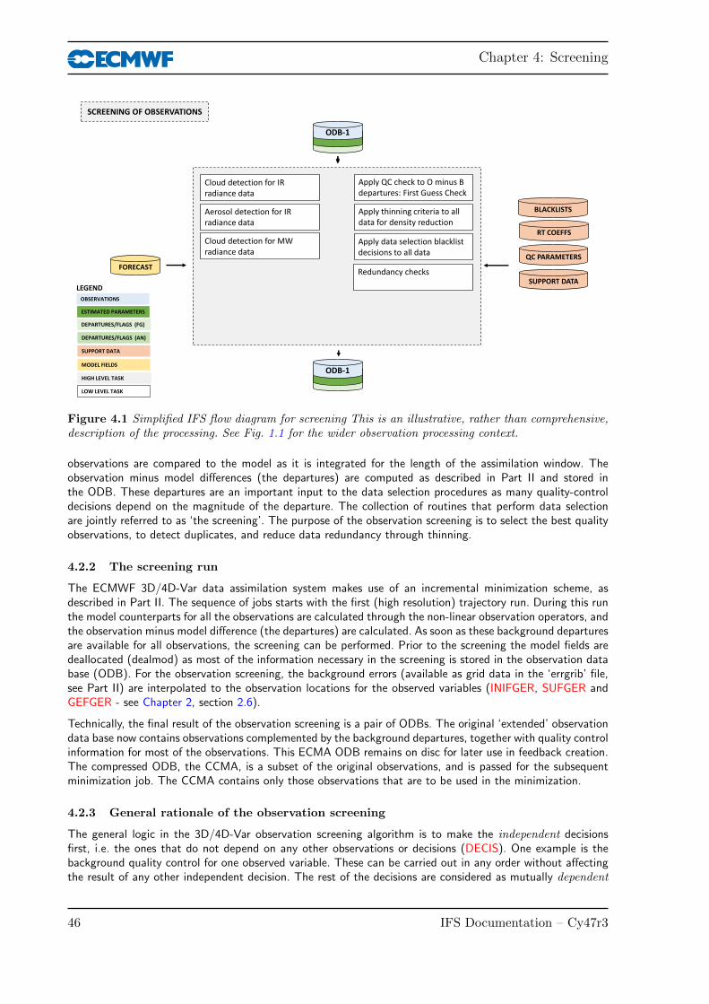
Chapter 4: Screening
ODB-1
SCREENING OF OBSERVATIONS
LEGEND
OBSERVATIONS
DEPARTURES/FLAGS (FG)
MODEL FIELDS
SUPPORT DATA
ESTIMATED PARAMETERS
HIGH LEVEL TASK
LOW LEVEL TASK
DEPARTURES/FLAGS (AN)
ODB-1
Cloud detection for IR radiance data
Aerosol detection for IR radiance data
Apply QC check to O minus B departures: First Guess Check
Apply thinning criteria to all data for density reduction
SUPPORT DATA
QC PARAMETERS
RT COEFFSCloud detection for MW radiance data
Apply data selection blacklist decisions to all data
BLACKLISTS
FORECASTRedundancy checks
Figure 4.1 Simplified IFS flow diagram for screening This is an illustrative, rather than comprehensive,description of the processing. See Fig. 1.1 for the wider observation processing context.
observations are compared to the model as it is integrated for the length of the assimilation window. Theobservation minus model differences (the departures) are computed as described in Part II and stored inthe ODB. These departures are an important input to the data selection procedures as many quality-controldecisions depend on the magnitude of the departure. The collection of routines that perform data selectionare jointly referred to as ‘the screening’. The purpose of the observation screening is to select the best qualityobservations, to detect duplicates, and reduce data redundancy through thinning.
4.2.2 The screening run
The ECMWF 3D/4D-Var data assimilation system makes use of an incremental minimization scheme, asdescribed in Part II. The sequence of jobs starts with the first (high resolution) trajectory run. During this runthe model counterparts for all the observations are calculated through the non-linear observation operators, andthe observation minus model difference (the departures) are calculated. As soon as these background departuresare available for all observations, the screening can be performed. Prior to the screening the model fields aredeallocated (dealmod) as most of the information necessary in the screening is stored in the observation database (ODB). For the observation screening, the background errors (available as grid data in the ‘errgrib’ file,see Part II) are interpolated to the observation locations for the observed variables (INIFGER, SUFGER andGEFGER - see Chapter 2, section 2.6).
Technically, the final result of the observation screening is a pair of ODBs. The original ‘extended’ observationdata base now contains observations complemented by the background departures, together with quality controlinformation for most of the observations. This ECMA ODB remains on disc for later use in feedback creation.The compressed ODB, the CCMA, is a subset of the original observations, and is passed for the subsequentminimization job. The CCMA contains only those observations that are to be used in the minimization.
4.2.3 General rationale of the observation screening
The general logic in the 3D/4D-Var observation screening algorithm is to make the independent decisionsfirst, i.e. the ones that do not depend on any other observations or decisions (DECIS). One example is thebackground quality control for one observed variable. These can be carried out in any order without affectingthe result of any other independent decision. The rest of the decisions are considered as mutually dependent
46 IFS Documentation – Cy47r3

Part I: Observations
on other observations or decisions, and they are taken next, following a certain logical order. For instance, thehorizontal thinning of radiance reports is only performed for the subset of reports that passed the backgroundquality control. Finally, the CCMA database is created for the minimization in such a way that it only containsthe data that will be used.
4.2.4 3D-Var versus 4D-Var screening
In the original 3D-Var assimilation system the screening rules were applied once, for the complete set ofobservations spanning a six-hour period. In the early implementation of the 4D-Var assimilation system, thesame data selection approach called ‘3D-screening’ was applied over the 6-hour long 4D-Var time window,which resulted in essentially the same screening decisions as in 3D-Var.
In summer 1997, a new screening procedure called 4D-screening was implemented that took into account thetemporal distribution of the observations. The time window is divided into time-slots of typically half-hourlength (15 minutes for the first and the last time slots). The 3D-screening algorithm was then applied separatelyto observations within each time-slot. This allowed more data to be used by 4D-Var, for instance, all messagesfrom an hourly reporting station can now be used, whereas only one (closest to central time) would havebeen allowed by the redundancy check in the 3D-screening. The 4D-screening behaviour is activated by switchLSCRE4D; it is meant to be used in conjunction with time correlation of observation errors where appropriate,as explained in Jarvinen et al. (1999) and in Part II.
4.3 SCREENING DECISIONS MADE IN OBSERVATION OPERATORS
Many screening decisions are easiest to make in the observation operator itself, and are performed under thecondition LSCREEN=.TRUE.
4.3.1 Satellite radiances
(a) Cloud and rain rejection for clear-sky observations
For data assimilated through the clear-sky route in the IFS, observations contaminated by significant cloud orrain signals must be removed before being supplied to the 4D-Var minimization in the clear-sky assimilationscheme. Microwave radiances that are assimilated in all-sky conditions are not subject to cloud or rain rejection.
For clear-sky microwave radiances (e.g. ATMS) cloud/rain screening is performed in the routineMW CLEARSKY SCREEN. This requires observation departures and is presently called from DEPAR-TURE JO. In addition to departures in window channels, it also uses retrievals of liquid water path or scatterindices derived from the observations.
For infrared radiances the test for clouds is done in routine CLOUD DETECT for AIRS/IASI and routineHIRS CLD for HIRS. The former is based on the algorithm described in McNally and Watts (2003). The latteris described in Krzeminski et al. (2009b). In both cases the aim is to identify which infrared channels can beused in a particular scene and which must be rejected.
For both the microwave and infrared data, if an observation is rejected due to cloud contamination, thecontam cld flag is set in the datum event1 field in the ODB. These observations will not influence any aspectsof the analysis including bias parameter evolution in the VARBC.
There is a special case of infrared cloud contamination that does not lead to channels being rejected. Inparallel to the setting of clear and cloudy flags, simplified cloud parameters (cloud top pressure and effectivecloud fraction are estimated from the infrared data (HIRS, AIRS and IASI) in routine CLOUD ESTIMATE.In the case that a pixel is diagnosed as completely overcast and subject to some additional restrictions placedupon the altitude of the diagnosed cloud (e.g. that it is not within 100hPa of the surface), the rejection flagsare NOT set. All channels in that pixel are then assimilated with the estimated cloud parameters passed tothe forward operator and further evolved as local extensions to the control vector in the minimization. Theadditional use of overcast infrared radiances can be disabled by setting the logical variable LCLDSINK to false.
IFS Documentation – Cy47r3 47
Chapter 4: Screening
(b) All-sky radiances
Most data selection decisions for all-sky radiances are made within the observation operator code underMWAVE SCREEN and recorded in the ODB column DATUM TBFLAG (see Chapter 3).
4.3.2 Ground-based radar precipitation composites
Some additional screening is performed inside the observation operator for the NCEP Stage IV surfaceprecipitation observations (routine GBRAD SCREEN). Both sea points and points likely to be affected by theoccurrence of atmospheric ducting are flagged as rejected. Ducting which leads to the undesirable deflection ofradar beams towards the ground is diagnosed from vertical gradients of atmospheric refractivity, as computedfrom model temperature and moisture fields in routine GBRAD REFRAC (Lopez, 2011). In addition, pointswith background departures exceeding 1.5 in log(RR[mm/h]+1) space are also discarded from the assimilation.
4.4 GENERIC INDEPENDENT OBSERVATION SCREENINGDECISIONS
4.4.1 Preliminary check of observations
The observation screening begins with a preliminary check of the completeness of the reports (PRECH). Noneof the following values should be missing from a report: observed value, background departure, observationerror and vertical coordinate of observation. Also a check for a missing station altitude is performed for SYNOP,TEMP and PILOT reports. The reporting practice for SYNOP and TEMP mass observations (surface pressureand geopotential height) is checked (REPRA), as explained in Appendix A. At this stage also, the observationerror for SYNOP geopotential observations is inflated if the reported level is far from the true station level(ADDOER). The inflation is defined as a proportion of the difference between the reported level and the truestation altitude by adding 2% of the height difference to the observation error.
4.4.2 Blacklisting
Next, the observations are scanned through for blacklisting (subroutine BLACK). At the set-up stage theblacklist interface is initialized (BLINIT) to the external blacklist library. The blacklist files consist formallyof two parts. Firstly, the selection of variables for assimilation is specified in the ‘data selection’ part of theblacklist file. This controls which observation types, variables, vertical ranges etc. will be selected for theassimilation. Some more complicated decisions are also performed through the data selection file; for instance,an orographic rejection limit is applied in the case of the observation being too deep inside the model orography.This part of the blacklist also provides a handy tool for experimentation with the observing system, as wellas with the assimilation system itself. Secondly, a ‘monthly monitoring’ blacklist file is provided for discardingthe stations that have recently been reporting in an excessively noisy or biased manner compared with theECMWF background field.
Most data selection criteria are coded in so called blacklist files, written in a convenient, readable blacklistlanguage (see the Blacklist Documentation, Jarvinen et al., 1996). The blacklist mechanism is very flexibleand allows nearly complete control of which data to use/not use in the assimilation. The ‘monthly blacklist’is the part of the blacklist that is based on operational data monitoring results, and it is maintained by theMeteorological Operations Section. The blacklist is consulted in the screening job. The interface is set up inBLINIT, in such a way that a number of named items from the header (Table 4.1) and body (Table 4.2) partsof the observation report can be passed to the blacklist software. Depending on the blacklisting criteria flags arecommunicated to the routine BLACK, and those are written to the ECMA ODB data base. Blacklist-rejecteddata are subsequently excluded from the CCMA ODB and will not be present in the minimisation job steps.Data selection rules should be coded in the blacklist files whenever possible rather than in the IFS code itself.The operational blacklist history is kept in an archive.
(a) Scatterometer blacklisting decisions
In order to screen on sea-ice contamination, scatterometer data are removed (within the blacklist mechanism)whenever the model sea-ice fraction exceeds 1% or the model sea-surface-temperature analysis is below273.15 K. Land is removed by imposing that the model land-sea mask should not exceed 10%.
48 IFS Documentation – Cy47r3
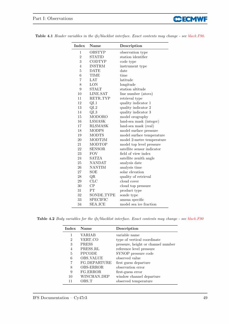
Part I: Observations
Table 4.1 Header variables in the ifs/blacklist interface. Exact contents may change - see black.F90.
Index Name Description
1 OBSTYP observation type2 STATID station identifier3 CODTYP code type4 INSTRM instrument type5 DATE date6 TIME time7 LAT latitude8 LON longitude9 STALT station altitude10 LINE SAT line number (atovs)11 RETR TYP retrieval type12 QI 1 quality indicator 113 QI 2 quality indicator 214 QI 3 quality indicator 315 MODORO model orography16 LSMASK land-sea mask (integer)17 RLSMASK land-sea mask (real)18 MODPS model surface pressure19 MODTS model surface temperature20 MODT2M model 2-metre temperature21 MODTOP model top level pressure22 SENSOR satellite sensor indicator23 FOV field of view index24 SATZA satellite zenith angle25 NANDAT analysis date26 NANTIM analysis time27 SOE solar elevation28 QR quality of retrieval29 CLC cloud cover30 CP cloud top pressure31 PT product type32 SONDE TYPE sonde type33 SPECIFIC amsua specific34 SEA ICE model sea ice fraction
Table 4.2 Body variables for the ifs/blacklist interface. Exact contents may change - see black.F90
Index Name Description
1 VARIAB variable name2 VERT CO type of vertical coordinate3 PRESS pressure, height or channel number4 PRESS RL reference level pressure5 PPCODE SYNOP pressure code6 OBS VALUE observed value7 FG DEPARTURE first guess departure8 OBS-ERROR observation error9 FG ERROR first-guess error10 WINCHAN DEP window channel departure11 OBS T observed temperature
IFS Documentation – Cy47r3 49
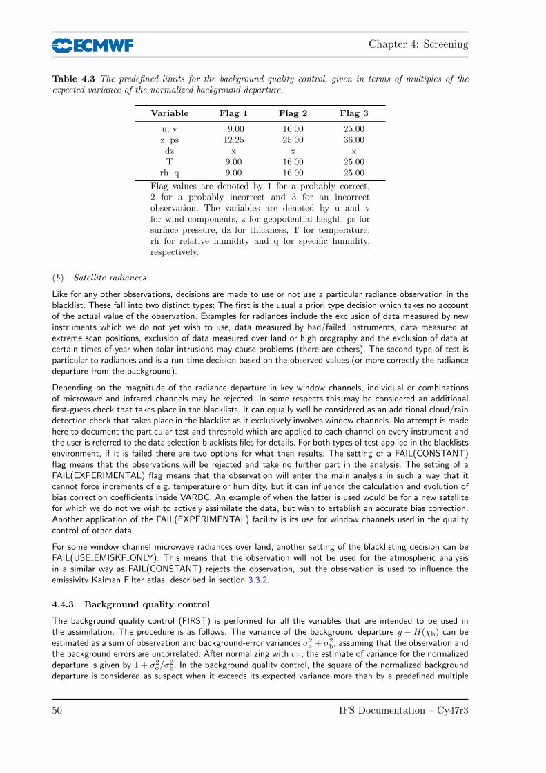
Chapter 4: Screening
Table 4.3 The predefined limits for the background quality control, given in terms of multiples of theexpected variance of the normalized background departure.
Variable Flag 1 Flag 2 Flag 3
u, v 9.00 16.00 25.00z, ps 12.25 25.00 36.00dz x x xT 9.00 16.00 25.00
rh, q 9.00 16.00 25.00
Flag values are denoted by 1 for a probably correct,2 for a probably incorrect and 3 for an incorrectobservation. The variables are denoted by u and vfor wind components, z for geopotential height, ps forsurface pressure, dz for thickness, T for temperature,rh for relative humidity and q for specific humidity,respectively.
(b) Satellite radiances
Like for any other observations, decisions are made to use or not use a particular radiance observation in theblacklist. These fall into two distinct types: The first is the usual a priori type decision which takes no accountof the actual value of the observation. Examples for radiances include the exclusion of data measured by newinstruments which we do not yet wish to use, data measured by bad/failed instruments, data measured atextreme scan positions, exclusion of data measured over land or high orography and the exclusion of data atcertain times of year when solar intrusions may cause problems (there are others). The second type of test isparticular to radiances and is a run-time decision based on the observed values (or more correctly the radiancedeparture from the background).
Depending on the magnitude of the radiance departure in key window channels, individual or combinationsof microwave and infrared channels may be rejected. In some respects this may be considered an additionalfirst-guess check that takes place in the blacklists. It can equally well be considered as an additional cloud/raindetection check that takes place in the blacklist as it exclusively involves window channels. No attempt is madehere to document the particular test and threshold which are applied to each channel on every instrument andthe user is referred to the data selection blacklists files for details. For both types of test applied in the blacklistsenvironment, if it is failed there are two options for what then results. The setting of a FAIL(CONSTANT)flag means that the observations will be rejected and take no further part in the analysis. The setting of aFAIL(EXPERIMENTAL) flag means that the observation will enter the main analysis in such a way that itcannot force increments of e.g. temperature or humidity, but it can influence the calculation and evolution ofbias correction coefficients inside VARBC. An example of when the latter is used would be for a new satellitefor which we do not we wish to actively assimilate the data, but wish to establish an accurate bias correction.Another application of the FAIL(EXPERIMENTAL) facility is its use for window channels used in the qualitycontrol of other data.
For some window channel microwave radiances over land, another setting of the blacklisting decision can beFAIL(USE EMISKF ONLY). This means that the observation will not be used for the atmospheric analysisin a similar way as FAIL(CONSTANT) rejects the observation, but the observation is used to influence theemissivity Kalman Filter atlas, described in section 3.3.2.
4.4.3 Background quality control
The background quality control (FIRST) is performed for all the variables that are intended to be used inthe assimilation. The procedure is as follows. The variance of the background departure y −H(χb) can beestimated as a sum of observation and background-error variances σ2
o + σ2b, assuming that the observation and
the background errors are uncorrelated. After normalizing with σb, the estimate of variance for the normalizeddeparture is given by 1 + σ2
o/σ2b. In the background quality control, the square of the normalized background
departure is considered as suspect when it exceeds its expected variance more than by a predefined multiple
50 IFS Documentation – Cy47r3

Part I: Observations
(FGCHK, SUFGLIM). For the wind observations, the background quality control is performed simultaneouslyfor both wind components (FGWND). In practice, there is an associated background quality-control flag withfour possible values, namely 0 for a correct, 1 for a probably correct, 2 for a probably incorrect and 3 foran incorrect observation, respectively (SUSCRE0). Table 4.3 gives the predefined limits for the backgroundquality control in terms of multiples of the expected variance of the normalized background departure. Thesevalues are set in DEFRUN and can be changed in namelist NAMJO. For SATOB winds the background errorlimits are modified as explained in Appendix A.
There is also a background quality control for the observed wind direction (FGWND). The predefined errorlimits of 60, 90 and 120 apply for flag values 1, 2 and 3, respectively. The background quality controlfor the wind direction is applied only above 700 hPa for upper-air observations for wind speeds larger than15 ms−1. If the wind-direction background quality-control flag has been set to a value that is greater than orequal to 2, the background quality-control flag for the wind observations is increased by 1.
There is no first-guess check for scatterometer data. It is demanded, though, that neither scatterometer normodel wind speed should exceed 35 ms−1, since that marks the range of validity for scatterometer windinversion.
4.5 THE DEPENDENT OBSERVATION SCREENING DECISIONS
4.5.1 Update of the observations
Just before performing the dependent screening decisions, the flag information gathered so far is convertedinto a status of the reports, namely: active, passive, rejected or blacklisted, and also into a status ofthe data in the reports (FLGTST). The reports with a RDB report flag value 2 (probably incorrect) or higherfor latitude, longitude, date and time are rejected. For the observed data there are RDB datum flags for thevariable and for the pressure, i.e. the pressure level of the observation. The rejection limits for these are asfollows: all data are rejected for the maximum RDB datum flag value 3 (incorrect), non-standard-level dataare rejected for the maximum RDB datum flag value 2, and for the pressure RDB datum flag the rejectionlimit is 1 (probably correct). The background quality control rejection limits are flag value 3 for all the data,and flag value 2 for the non-standard-level data.
4.5.2 Global time–location arrays
Some of the dependent decisions require a global view to the data which is not available as the memory isdistributed. Therefore ad hoc global time–location arrays are formed and broadcast in order to provide thisview (GLOBA, DISTR).
4.5.3 Vertical consistency of multilevel reports
The first dependent decisions are the vertical-consistency check of multilevel reports (VERCO), and the removalof duplicated levels from the reports. The vertical-consistency check of multilevel reports is applied in sucha way that if four consecutive layers are found to be of suspicious quality, even having a flag value one,then these layers are rejected, and also all the layers above these four are rejected in the case of geopotentialobservations. These decisions clearly require the quality-control information, and they are therefore ‘dependent’on the preceding decisions.
4.5.4 Removal of duplicated reports
The duplicated reports will be removed next. That is performed (MISCE, DUPLI, REDSL) by searching pairsof collocated reports of the same observation types, and then checking the content of these reports. It may, forinstance, happen that an airep report is formally duplicated by having a slightly different station identifier butwith the observed variables inside these reports being exactly the same, or partially duplicated. The pair-wisechecking of duplicates results in a rejection of some or all of the content of one of the reports.
IFS Documentation – Cy47r3 51
Chapter 4: Screening
4.5.5 Redundancy check
The redundancy check of the reports, together with the level selection of multi-level reports, is performed nextfor the active reports that are collocated and that originate from the same station (REDUN). In 3D-screening,this check applies to the whole observation time window. In 4D-screening (LSCRE4D = .TRUE.), this checkapplies separately in each timeslot.
For LAND SYNOP and PAOB reports, the report closest to the analysis time with most active data isretained, whereas the other reports from that station are considered as redundant and are therefore rejectedfrom the assimilation (REDRP, REDMO). For SHIP SYNOP and DRIBU observations the redundancycheck is done in a slightly modified fashion (REDGL). These observations are considered as potentiallyredundant if the moving platforms are within a circle with a radius of 1 latitude. Also in this case onlythe report closest to the analysis time with most active data is retained. All the data from the multilevelTEMP and PILOT reports from same station are considered at the same time in the redundancy check(REDOR, SELEC). The principle is to retain the best quality data in the vicinity of standard levels and closestto the analysis time. One such datum will, however, only be retained in one of the reports. A wind observation,for instance, from a sounding station may therefore be retained either in a TEMP or in a PILOT report,depending on which one happens to be of a better quality. A SYNOP mass observation, if made at thesame time and at the same station as the TEMP report, is redundant if there are any TEMP geopotentialheight observations that are no more than 50 hPa above the SYNOP mass observation (REDSM).
4.5.6 Thinning
Finally, a horizontal thinning is performed for the AIREP, radiances (ATOVS,AIRS,IASI), GEOS, SATOB,ERS and SCAT SCAT reports. The horizontal thinning of reports means that a predefined minimum horizontaldistance between the nearby reports from the same platform is enforced. For AIREP reports the free distancebetween reports is currently enforced to about 60 km (Cardinali et al., 2003). The thinning of the AIREP datais performed with respect to one aircraft at a time (MOVPL, THIAIR). Reports from different aircraft mayhowever be very close to each other. In this removal of redundant reports the best quality data is retained asthe preceding quality controls are taken into account. In vertical, the thinning is performed for layers aroundmodel levels, thus allowing more reports for ascending and descending flight paths.
Thinning of radiances, GRAD, SATOB, ERS and ASCAT SCAT reports are each done in two stages controlledby THINN. For radiances (THINNER), a minimum distance of about 70 km is enforced and, thereafter, arepeat scan is performed to achieve the final separation of roughly 250 km or 120 km between reports fromone platform. This is controlled through settings in DEFRUN, that can also be modified through namelist(NAMSCC). The thinning algorithm is the same as used for AIREPs except that for radiances a differentpreference order is applied: a sea sounding is preferred over a land one, a clear sounding is preferred over acloudy one and, finally, the closest observation time to the analysis time is preferred. For geostationary watervapour radiances, a similar thinning in two stages is applied with currently about 70 km minimum distance andabout 125 km final separation (THINNER). During the thinning, preference is given to data having the largestfraction of clear sky in the clear-sky radiance average, high infrared brightness temperature (for GOES data)and, finally, a small standard deviation of brightness temperatures within the CSR mean. A similar thinningtechnique is applied to SATOB high-density data (THINNER). Note that prior to assimilation a coarser pre-thinning may take place already during observation pre-processing in order to reduce otherwise excessive datavolumes.
The screening of SATOB data has been extended for atmospheric motion wind observations, includingindividual quality estimate. The quality information from the quality control performed by the producer atextraction time is appended to each wind observation. This Quality Indicator (QI) is introduced as an additionalcriterion in the thinning step; priority is given to the observation with the highest QI value.
For ERS and ASCAT scatterometer data, the above described thinning algorithm is only applied along track.In across-track direction, backscatter data from these platforms are provided into wind-vector cells (WVC)with a spatial resolution of 25 km. In this direction, data is thinned by selecting predefined wind-vector cells(subroutine SCAQC). For ERS, from 19 cells, only 3, 7, 11, 15 and 19 are regarded (cells 1 and 2 are of knownlower quality). For ASCAT, from 42 cells (two swaths of 21 cells each) only cells 1, 5, 9, 13, 17, 21, 22, 26,30, 34, 38 and 42 are used. After this across-track thinning, the generic thinning algorithm is applied to the
52 IFS Documentation – Cy47r3

Part I: Observations
remaining cells in along-track direction. QuikSCAT data (also provided on a 25 km grid) are not thinned.Instead, a 50 km wind product is determined from backscatter data from four underlying 25 km cells, eachgiven a reduced weight of one fourth.
Scatterometer winds are besides thinning subject to a high-wind rejection test with an upper-wind speed limitset to 35 ms−1 to both the scatterometer and background winds (FGWND).
4.5.7 Compression of the ODB
After the observation screening roughly a fraction of 1/10 of all the observed data are active and so thecompressed observation ODB (the CCMA) for the minimization run only contains those data. The largecompression rate is mainly driven by the number of radiance data, since after the screening there are only10–20% of the radiance reports left, whereas for the conventional observations the figure is around 40%. Asa part of the compression, the observations are re-sorted amongst the processors for the minimization job inorder to achieve a more optimal load balancing of the parallel computer.
4.6 PARALLEL ASPECTS
As mentioned earlier, in the observation screening there are the two basic types of decision to be made.Independent decisions, on one hand, are those where no information concerning any other observation ordecision is needed. In a parallel-computing environment these decisions can be happily made by differentprocessors fully in parallel. For dependent decisions, on the other hand, a global view of the observations isneeded which implies that some communication between the processors is required. The observation array is,however, far too large to be copied for each individual processor. Therefore, the implementation of observationscreening at the ECMWF is such that only the minimum necessary information concerning the reports iscommunicated globally.
The global view of the observations is provided in the form of a global ‘time–location’ array for selectedobservation types. That array contains compact information concerning the reports that are still active at thisstage. For instance, the observation time, location and station identifier as well as the owner processor ofthat report are included. The time–location array is composed at each processor locally and then collected formerging and redistribution to each processor. After the redistribution, the array is sorted locally within theprocessors according to the unique sequence number. Thus, every processor has exactly the same informationto start with, and the dependent decisions can be performed in a reproducible manner independently of thecomputer configuration.
The time–location array is just large enough for all the dependent decisions, except for the redundancy checkingof the multilevel TEMP and PILOT reports. This is a special case, in the sense that the information concerningeach and every observed variable from each level is needed. Hence, the whole multilevel report has to becommunicated. The alternative to this would be to force the observation clusters of the multilevel reportsalways into one processor without splitting them. In that case the codes responsible for the creation of theobservation arrays for assimilation would need to ensure the geographical integrity of the observation arraysdistributed amongst the processors. This is, however, not possible in all the cases, and the observation screeninghas to be able to cope with this. Currently, it is coded in such a way that only a limited number of multilevelTEMP and PILOT reports, based on the time–location array, are communicated between the appropriateprocessors as copies of these common stations.
APPENDIX A
A.1 Bad reporting practice of SYNOP and TEMP reports
The way the synoptic surface stations report mass observations (pressure or geopotential height) is consideredas bad if:
• station altitude is above 800 m and station reports mean sea level pressure• station altitude is above 800 m and station reports 1000 hPa level• station altitude is above 1700 m and station reports 900 hPa level• station altitude is below 300 m and station reports 900 hPa level
IFS Documentation – Cy47r3 53
Chapter 4: Screening
• station altitude is above 2300 m and station reports 850 hPa level• station altitude is below 800 m and station reports 850 hPa level• station altitude is above 3700 m and station reports 700 hPa level• station altitude is below 2300 m and station reports 700 hPa level• station altitude is below 3700 m and station reports 500 hpa level
The reporting practice is also considered as bad if the station reports 500 gpm, 1000 gpm, 2000 gpm, 3000 gpmor 4000 gpm level pressure, respectively, and station altitude is more than 800 m different from the reportedlevel.
For TEMP geopotentials the reporting practice is considered as bad if:
• station altitude is above 800 m and station reports 1000 hPa level• station altitude is above 2300 m and station reports 850 hPa level• station altitude is above 3700 m and station reports 700 hPa level
A.2 Revised background quality control for selected observations
The background quality-control rejection limits are applied more strictly for some observation types than statedin Table 4.3. The special cases are the following ones.
• AIREP wind observations with zero wind speed are rejected if the background wind exceeds 5 m s−1.• For AIREP and DRIBU wind observations the rejection limit is multiplied by 0.5, and for PILOT wind
by 0.8.• For SATOB wind observations the rejection limit is multiplied by 0.1, except below 700 hPa level where
it is multiplied by 0.2.• No background quality control is applied for SCAT winds.• For DRIBU surface pressure observations the rejection limit is multiplied by 0.9, and for PAOB surface
pressure by 0.7.• For AIREP temperature observations the rejection limit is multiplied by 1.6.
54 IFS Documentation – Cy47r3
Part I: Observations
Chapter 5
Deprecated areas
Table of contents5.1 Introduction
5.2 Continuous Observation Processing Environment (COPE) transition
5.3 MKCMARPL tasks and functions [DEPRECATED]
5.3.1 Basic observation processing setup [DEPRECATED]
5.3.2 Invoking, initializing and controlling the MKCMARPL [DEPRECATED]
5.3.3 MKCMARPL [DEPRECATED]
5.3.4 Basic observation handling routines [DEPRECATED]
5.1 INTRODUCTION
This section is for deprecated parts of the observation code, things which have increasingly little relevance tounderstanding the modern system. Unfortunately, the deprecated code still performs a few important tasks,otherwise it would have already been removed. This documentation is not kept up to date but it is still usefulfor understanding those few remaining tasks, especially for those people whose job it will be to replace themcompletely.
The main deprecated area is ‘Make CMA replacement’ or MKCMARPL which once performed most of thepre-processing tasks in the IFS. Nowadays, pre-processing for conventional in-situ observations has largely beensuperseded by COPE (what remains is Meteo-France specific). However, a number of other observation typesstill rely on MKCMARPL in important ways, or just in annoying ways that make it hard to simply delete whatis apparently useless code. For example:
• AMVs require variable conversion from windspeed and direction to horizontal wind components u andv. More pointlessly, they also need to set up an (unused) initial observation error using the deprecatedOBSERR routines. This error needs to be present in the ODB to prevent rejection during screening,even though it is not used.
• For some satellite radiances, channel numbering is reassigned. There may or may not be anything elseuseful going on under LEVEL1CGEOS OB. for example, there are checks on longitudes, latitudes andtimes, but these are likely duplicates of checks elsewhere in the pre-processing.
• Scatterometer processing still relies on the MKCMARPL. The retrieval from backscatter to winds, andre-ordering of the observation body elements.
• Ozone observations still rely on MKCMARPL. Among other things they set up observation errors here.
5.2 CONTINUOUS OBSERVATION PROCESSING ENVIRONMENT(COPE) TRANSITION
The following is an alphabetical list of all subroutines, modules and module variables that have been deprecatedand that are planned to be removed from IFS in one of the future cycles, or have already been removed:
AIREPBE, AIREPIN, AWPRFIN, BIASCOR ODB, CONVENTIONAL OB, DRIBUBE, DRIBUIN, ERR-STAT, EWPRFIN, FINOEREV, FIXERR, GET NEW RS TRH BIAS, GET RS T BIAS, HATBIASC,LNDSYIN, METARIN, NEW RS TRH BIAS, OBINSTP, OBSERR, PGPSIN, PILOTBE, PILOTIN, PRLM-CHK, PTENDCOR, REPSEL, RH2Q, RS BIAS VALIDITY, SHIPIN, SONDE COUNTRY DB MATCH,
IFS Documentation – Cy47r3 55

Chapter 5: Deprecated areas
SULEVLAY, SUOBSERR, SYNOPBE, SYNOPIN, TEMPBE, TEMPIN, YOMLVLY, YOMMKODB:LCD[0-9]*, YOMMKODB:NMKCMVSE, YOMOERR, YOMOBS:LMKCMARPL, YOMRSTRHBIAS, Z2PICAO.
Note that some of these (for example OBSERR and ERRSTAT) are still used by, for example, the AMVs.
Additionally, some of the subroutines considered to be completely obsolete were not reimplemented in COPEframework. These include PTENDCOR formerly used for ship surface pressure adjustment (Subsection 2.4.3)and subroutines GET RS T BIAS, HATBIASC, BIASCOR ODB, RS BIAS VALIDITY and BIASCOR usedfor old style radiosonde temperature and humidity bias correction. These subroutines are not likely to bereimplemented in COPE unless there is a specific need to do so.
The following listing should give some pointers as to where to find particular MKCMARPL functionalitieswithin the COPE framework. On the left side (red font) are former IFS Fortran subroutines and, on the right(bold font), their corresponding counterparts in COPE framework. Note that this is only represents a loosemapping where applicable:
• AIREPIN — airep.json• DRIBUIN — dribu.json• TEMPIN — temp.json• PILOTIN — pilot.json• PGPSIN — pgps.json• LNDSYIN — synop.json• SHIPIN — ship.json• AWPRFIN — awp.json• EWPRFIN — ewp.json• PRLMCHK — DateTimeValidator, LocationValidator• YOMOERR, SUOBSERR — error statistics.csv• YOMLVLY, SULEVLAY, ERRSTAT, OBSERR, FIXERR — PrescribedErrorAssigner• FINOEREV — FinalErrorAssigner• RH2Q — SpecificHumidityAssigner• OBINSTP — InstrumentTypeAssigner• Z2PICAO — HeightToPressureConverter• YOMRSTRHBIAS, GET NEW RS TRH BIAS, SONDE COUNTRY DB MATCH, NEW RS TRH BIAS
— RadiosondeBiasCorrector
As can be seen in the listing above, there is nearly one to one correspondence between the former MKCMARPLworker Fortran subroutines [A-Z]*IN and [a-z]*.json configuration files. This is not by coincidence sincepreserving the former logical structure makes the transition to new framework more transparent. The JSONconfiguration files describe processing pipeline for the given observation type in declarative way. This allowsto modify or even construct new pipelines at runtime, reusing existing filters, without having to recompile thesource. Conceptually, every pipeline is composed of a chain of filters that are sequentially applied on eachobservation report. All JSON configuration files can be found in the standard IFS scripts directory.
5.3 MKCMARPL TASKS AND FUNCTIONS [DEPRECATED]
5.3.1 Basic observation processing setup [DEPRECATED]
In order to perform the observation processing functions, a number of basic observation processing setups arecarried out at the very beginning of initialising the IFS. This is done by calling several routines in addition toall other routines needed to setup the IFS.
• Program MASTER calls CNT0 which in turn calls SU0YOMA.• SU0YOMA calls (among other routines) SUOAF from which SUCMOCTP, SUEVENTS, SUCODES,
SUFLTXT and SUCMA are called. SUCMOCTP defines the ODB observation types and code types,and SUEVENTS, SUCODES and SUFLTXT define analysis events, various codes used and flags namingconventions.
• SUCMA calls SUCMAF which then calls several subroutines: SUCMAD1, SUCMAD2, SUCMAHFP,SUCMAHOP, SUCMBDFP and SUCMBDTP. These routines define the structure of ODB Data
56 IFS Documentation – Cy47r3

Part I: Observations
Descriptor Records (DDRs) as well as the ODB packing patterns (bit structure) employed for headerand body respectively.
5.3.2 Invoking, initializing and controlling the MKCMARPL [DEPRECATED]
The MKCMARPL run is initiated by the MKCMARPL subroutine. This routine is only invoked in theSCREENING run of the IFS. It is called, together with some of its additional setup routines via subroutineSUOBS. The additional setup routines called at this level are: SUANCT, DEFRUN, SULIM, SULEVLAY,SUSATRET, SUVNMB, SUSCRE0, SUOBSORT, SETCOM, DEPERERR, SUERRORS, INIERSCA.
• MKCMARPL is namelist driven and in DEFRUN a logical variable LMKCMARPL is defined. By defaultLMKCMARPL = .TRUE. but it can be overwritten via namelist NAMOBS. Furthermore, many otherparameters and switches are defined in DEFRUN and some of them can also be overwritten via namelists.
• SUANCT and SULIM define some additional analysis constants and limits.• SULEVLAY and SUSATRET define analysis related level/layer and satellite retrieval parameters,
respectively.• SUVNMB declares variable numbers.• SUSCRE0, SUOBSORT and SETCOM define flag limits, identify ambiguous moving platforms, initialise
observation sorting, and provide some general observation common variables.• DEPERERR and SUERRORS deal with observation error statistics definitions. SUERRORS calls
SUPERERR to define observation persistence errors and SUOBSERR to define prescribed observationerrors.
• INIERSCA deals with initialising SCATT processing.
The next step is to find out if it is a SCREENING run and if so to check if it is a MKCMARPL run as well. Inthe case of a MKCMARPL run all aspects of the observation processing before the screening are dealt with bycalling MKCMARPL (more about it in Subsection 5.3.3). After MKCMARPL has finished there are several waysto proceed. These depend on the status of LMKCMARPLO and LRPLSWAPOUT logical switches (NAMOBSnamelist). If LRPLSWAPOUT= .TRUE. the ODB is swapped out and if LMKCMARPLO= .TRUE. theODB is written out and the run terminated. Both of these options are not normally used and their use is fordiagnostics/debugging purposes. Once the MKCMARPL work has been completed the remainder of SUOBSwill execute as before. Thus, calls to WRITEOBA, WINDAUX, OBATABS, SUAMV, SURAD, SULIMB,SUOBAREA, MKGLOBSTAB and SUREO3 are issued.
In the context of operational running, the MKCMARPL related switches are set:
LMKCMARPL = .TRUE. LRPLSWAPOUT= .FALSE. LMKCAMRPLO= .FALSE.
5.3.3 MKCMARPL [DEPRECATED]
WARNING: As of IFS cycle 41r1, majority of MKCMARPL tasks dealing with conventional observation pre-processing have been deprecated and their functionality has been migrated to COPE framework. Although theMKCMARPL has not been fully replaced yet, and can still be used, it is strongly recommended to do newdevelopments in the area of conventional observations within the COPE framework. For more details, includinga full list of deprecated subroutines, see Section 5.2.
The main purpose of MKCMARPL is to control the IFS observation pre-processing. Observation pre-processingat this stage is done in groups of observations. At the moment there are six groups: CONVENTIONAL,SATOB, TOVS/RTOVS, SCATT, LEVEL1C/GEOSS and OZONE observations. For each group a separatesubroutine is called: CONVENTIONAL OB, SATOB OB, TOVSRTOVS OB, SCAT OB, LEVEL1CGOES OBand OZONE OB. These routines are just cover or hat routines for the actual work to be carried out underneath.However, TOVSRTOVS OB is currently not called because it is obsolete.
Each cover routine would call the ODB to get the observations it wants to process. This is done by callingthe ODB GETDB subroutine. As the observations are brought, in one or more worker routines would be calledto perform the observation processing functions. Once the worker routines have finished the control is handedback to the cover routine. The next step in the cover routine is to return observations back to the ODBdatabase. This is done by calling the ODB PUTDB routine. In some of these cover routines several calls to
IFS Documentation – Cy47r3 57

Chapter 5: Deprecated areas
GETDB/PUTDB might be issued. This is because there may be sufficient differences between similar datato justify a slightly different approach in their pre-processing. For example under the CONVENTIONAL OBroutine there are two calls to a GETDB and PUTDB pair. The first call deals with all conventional observationsexcept SATEMs; the second call deals with the SATEMs. As indicated earlier, between each GETDB andPUTDB a number of observations type or code type designed worker routines are called.
• CONVENTIONAL OB calls the following worker routines: SYNOPIN, AIREPIN, DRIBUIN, TEMPIN,PILOTIN, EWPRFIN, AWPRFIN, PAOBIN and METARSIN. A worker routine name indicates whichobservations it is dealing with.
• SATOB OB calls SATOBIN and SATAMIN.• SCAT OB calls ERS1IN, NSCATIN, ASCATIN and QSCATIN.• LEVEL1CGEOS OB calls RAD1CIN and GOESRIN.• OZONE OB calls only REO3SIN.
5.3.4 Basic observation handling routines [DEPRECATED]
The observation pre-processing worker routines referred to in Subsection 5.3.3, names of which always endwith “IN”, are the basic observation handling routines. They all follow more or less the same logic. As anexample consider AIREPIN which deals with AIREP observations.
The first thing which is done is to define the instrument specification (OBINSTP) followed by preliminaryquality control check both at the report level (PRLMCHK) as well as at the data level (GETSETE andAIREPBE).
• PRLMCHK calls REPSEL and TIMDIF to do report selection according to preset criteria and to findout time difference between analysis time and the actual observation time, respectively.
• GETSETE makes a local copy of a given observation variable and its related parameters from an ODBsupplied array.
• After updating the local copy, AIREPBE is called to return the updated local copy back to the ODBsupplied array.
The preliminary quality control at the report level consists of making sure that observation position, date andtime are reasonable. Furthermore, as there is a possibility of excluding certain observations via the NAMOBSnamelist, a check is made of whether the observation is actually wanted at this stage. Once the report levelcheck is passed attention is turned to the data itself. Each datum is checked against predefined list of expecteddata. If not in the list, datum is rejected and a warning message issued. At this stage it is also ensured thatmissing indicators used are unique.
After the preliminary phase attention is turned to getting data in the right form and shape for further usage.Thus, in the case of an AIREP observation, this is done in sections of available variables: wind and temperature.
(i) Wind. There are four wind variables: wind direction (DDD), wind force (FFF), u and v components.For each of these variables the first thing which is done is to get a local copy of it together with its relatedparameters from an ODB supplied array (GETSETE). Once a variable is made available locally a check ismade to ensure that the vertical coordinate is pressure; if instead of pressure a flight level is supplied it isconverted into pressure by assuming a standard ICAO atmosphere (Z2PICAO). If the variable in questionis either u or v, then DDD and FFF are converted into u and v wind components. Furthermore, for eachof the four variables appropriate observation error statistics are assigned (ERRSTAT, FINOERR). Also,if any flags are set at this stage an appropriate word in the local copy is updated (PPVAFL). Finally, anupdated local copy of an observed quantity and its related parameters are returned back into the ODB(AIREPBE).
(ii) Temperature. In the case of temperature only one observed variable is dealt with. The pattern ofmaking a local copy (GETSETE), ensuring that pressure is the vertical coordinate (Z2PICAO), assigningthe observation error statistics (ERRSTAT), updating flags (PPVAFL) and returning an updated localcopy back to the ODB (AIREPBE) is repeated.
As just mentioned ERRSTAT deals with assigning observation errors for a given observation variable. ERRSTATfirst calls OBSPERR to assign observation persistence error; then it calls OBSERR which in turn calls FIXERR
58 IFS Documentation – Cy47r3

Part I: Observations
AIREPIN
OBINSTP
PRLMCHK
GETSETE
AIREPBE
GETSETE
Z2PICAO
FINOERR
ERRSTAT
PPVAFL
AIREPBE
GETSETE
Z2PICAO
ERRSTAT
AIREPBE
! Report (Header) Definition ! Report (Header) Check
! Data(Body) Check
! Wind Processing Section
! Temperature Processing Section
REPSEL
TIMDIF
FILFBDE
OBSPERR
OBSERR
FINOERR
FILFBDE
FIXERR
FILFBDE
OBSPERR
OBSERR
FINOERR
FIXERR
NGEDEVE
NGEDEVE
NGEDEVE
PPVAFL
Figure 5.1 Simplified IFS observation pre-processing flow diagram, with AIREPIN as an example. Colourcoding scheme: routines in red boxes perform observation pre-processing.
to assign prescribed observation error. It is worth mentioning that observation errors themselves are alreadypredefined at an earlier stage (SU ERRORS).
The pattern of activities outlined for AIREPIN is repeated more or less in the other worker routines. However,the SYNOPIN routine is first split further into SHIPIN, METARIN, PGPSIN and LANSYIN. This is becauseSHIP, METAR, GPS and SYNOP LAND observations are sufficiently different to justify a separate workerroutine. Furthermore, LANSYIN is somewhat more complicated than AIREPIN. One of the reasons for this isthat we have to distinguish between low and high level stations.
IFS Documentation – Cy47r3 59


Part I: Observations
Chapter 6
Tables, codes and flags
Table of contents6.1 Introduction
6.2 BUFR observation types and subtypes
6.3 Obstype and codetype
6.4 Variable codes (varno)
6.5 Conventional observation operator codes: NVAR and CVAR NAME - [DEPRECATED]
6.6 Observation characteristics: instrument specification and retrieval type
6.7 Vertical coordinate: pressure, satellite ID and level ID codes
6.8 ODB report status: events, flags and codes
6.9 Datum status: events, RDB and analysis flags
6.1 INTRODUCTION
Older versions of the IFS documentation have contained copious tables attempting to document all thecodes, flags and groupings for observations in the IFS. If this was ever possible, in recent years the variety ofobservational data processing has mushroomed, these tables have in some places became hopelessly out ofdate and their true counterparts are too large to comfortably fit in such documentation. The truest recordis the IFS source code, the ODB data archived to MARS, and the logfiles of the IFS. The ODB governancedatabase at http://apps.ecmwf.int/odbgov is reasonably up-to-date but does not cover everything. Someof the old tables from the IFS documentation are provided here, although no longer kept up-to-date, as theyare useful for illustration purposes, and as a guide to what these codes are for. See also Sec. 1.4.
6.2 BUFR OBSERVATION TYPES AND SUBTYPES
Although BUFR observation types and subtypes are not directly used in the IFS they are defined here. BUFRobservation types and subtypes are mapped into ODB observation types and code types before the IFS (i.e. theMERGEODB step). Some example BUFR observation types and subtypes are listed in Table 6.1. See WMOdocumentation for more, or the ODB governance tables http://data-portal.ecmwf.int/odbgov/
IFS Documentation – Cy47r3 61

Chapter 6: Tables, codes and flags
Table 6.1 Some BUFR observation types and subtypes. See WMO documentation for the full set, or theODB governance tables http://data-portal.ecmwf.int/odbgov/.
Observation Type Subtype
Code Name Code Name
0 Land Surface 1 Land SYNOP3 Automatic Land SYNOP9 Abbreviated Land SYNOP
110 GPS140 METAR
1 Sea Surface 9 SHIP11 SHIP13 Automatic SHIP19 Reduced SHIP21 DRIBU22 BATHY
2 Upper Air Sounding 91 Land PILOT92 SHIP PILOT95 Wind Profiler (American)96 Wind Profiler (European/Japanese)101 Land TEMP102 SHIP TEMPS103 DROP TEMP104 ROCOB105 SHIP ROCOB106 Mobile TEMP
3 Satellite Sounding 0 High Resolution TOVS51 High Resolution TOVS53 RTOVS54 ATOVS55 ATOVS57 ATOVS61 Low Level Temperature SATEM62 High Level SATEM63 PWC SATEM65 Merged SATEM71 Low Level TOVS72 High Level TOVS73 PWC TOVS75 Merged TOVS129 TRMM130 TMI161 PAOB206 OZONE Retrieved Layers
62 IFS Documentation – Cy47r3

Part I: Observations
Table 6.1 Continued.
Observation Type Subtype
Code Name Code Name
4 AIREP 142 AIREP143 COLBA144 AMDAR145 ACARS
5 SATOB 82 Temperature and Wind83 Wind Only84 Temperature only85 Temperature only86 High Resolution VIS Wind87 AMV89 Geostationary Clear Sky Radiances (GRAD)
189 Geostationary Clear Sky Radiances (GRAD)190 Geostationary All Sky Radiances (GRAD)
12 SCATT/SSMI 122 ERS-1, ERS-2127 SSMI136 NSCAT137 QSCAT139 ASCAT
253 PAOB 161 PAOB
IFS Documentation – Cy47r3 63

Chapter 6: Tables, codes and flags
Table 6.2 Some ODB observation types and code types. See the ODB governance tables http://data-portal.ecmwf.int/odbgov/ for a fuller and more up-to-date list
Observation Type Code Type
Code Name Code Name
1 SYNOP 11 Land SYNOP14 Automatic Land SYNOP16 French RADOME21 SHIP22 Abbreviated SHIP23 SHRED24 Automatic SHIP
140 METAR110 GPS
2 AIREP 41 CODAR141 AIREP142 Simulated AIREP144 AMDAR145 ACARS241 COLBA
3 SATOB 88 SATOB89 High Resolution VIS wind90 AMV
188 SST
4 DRIBU 63 BATHY64 TESAC
160 ERS as DRIBU165 DRIBU
5 TEMP 35 Land TEMP36 SHIP TEMP37 Mobile TEMP39 ROCOB40 SHIP ROCOB
135 DROP TEMP137 Simulated TEMP
6.3 OBSTYPE AND CODETYPE
There are also ODB ‘observation types’ and, as with BUFR, there are different number of code types for eachof them. It is reasonable to question why the BUFR and ODB observation types and sub or code types aredifferent. The answer is a historic one. The ODB observation types and code types have been used beforeBUFR came in to existence and as an international code it was difficult to impose our practice on the others.Also, there was not enough enthusiasm on our side to switch to the BUFR ones. Some ODB observation typesand code types are listed in Table 6.2. See the ODB governance tables http://data-portal.ecmwf.int/odbgov/for a fuller and more up-to-date list. The coexistence of different codes used for BUFR and ODB observationtypes and the subtype and code type requires a mapping from one to another. The ODB governance tablesalso describe that mapping.
64 IFS Documentation – Cy47r3

Part I: Observations
Table 6.2 Continued.
Observation Type Code Type
Code Name Code Name
6 PILOT 32 Land PILOT33 SHIP PILOT34 American Wind Profiler
131 Japanese Wind Profiler132 Mobile Wind Profiler134 European Wind Profiler
7 SATEM 86 GTS SATEM184 High Resolution Simulated TOVS185 High Resolution Simulated DWL SATEM186 High Resolution SATEM200 GTS BUFR SATEM 250km201 GTS BUFR Clear Radiances202 GTS BUFR Retrieved Profiles/Clear Radiances210 ATOVS/GRAD211 RTOVS212 TOVS215 SSMI
8 PAOB 164 PAOB
9 SCATTEROMETER 122 ERS-1, ERS-2210 NSCAT301 QuikSCAT139 ASCAT
10 RAW RADIANCE
IFS Documentation – Cy47r3 65

Chapter 6: Tables, codes and flags
Table 6.3 Some variables (VARNO) in the ODB. Check the ODB governance database http://data-portal.ecmwf.int/odbgov/ for the latest information.
No. Code Name Unit
1 3 Wind Component (u) ms−1
2 4 Wind Component (v) ms−1
3 1 Geopotential (Z) m2s−2
4 57 Thickness (DZ) m2s−2
5 29 Relative Humidity (RH) numeric
6 9 Precipitable Water Content (PWC) kgm−2
7 58 2 m Relative Humidity (RH 2m) numeric8 2 Temperature K9 59 Dew Point K10 39 2 m Temperature (T2m) K11 40 2 m Dew Point (Td2m) K12 11 Surface Temperature (Ts) K13 30 Pressure Tendency (Pt) Pa/3h14 60 Past Weather (W ) WMO Code 456115 61 Present Weather (WW) WMO Code 467716 62 Visibility (V ) WMO Code 430017 63 Type of High Clouds (CH) WMO Code 050918 64 Type of Middle Clouds (CM) WMO Code 051519 65 Type of Low Clouds (CL) WMO Code 051320 66 Cloud Base Height (Nh) m21 67 Low Cloud Amount (N) WMO Code 270022 68 Additional Cloud Group Height (hshs) m23 69 Additional Cloud Group Type (C) WMO Code 050024 70 Additional Cloud Group Amount (Ns) WMO Code 270025 71 Snow Depth (Sd) m26 72 State of Ground (E) WMO Code 090127 73 Ground Temperature (TgTg) K28 74 Special Phenomena (SpSp) WMO Code 377829 75 Special Phenomena (spsp) WMO Code 377830 76 Ice Code Type (Rs) WMO Code 355131 77 Ice Thickness (EsEs) WMO Code 175132 78 Ice (Is) WMO Code 175133 79 Time Period of Rain Information (trtr) hour
34 80 6 Hour Rain Amount kgm−2
35 81 Maximum Temperature (JJ) K36 82 Ship Speed (Vs) ms−1
37 83 Ship Direction (Ds) degree38 84 Wave Height (HwHw) m39 85 Wave Period (PwPw) s40 86 Wave Direction (DwDw) degree41 87 General Cloud Group WMO Code
6.4 VARIABLE CODES (VARNO)
To provide easy recognition of ‘observed’ variables each of them is assigned a numerical code. These codesare then embedded in ODB reports. For illustrative purposes some historical codes are listed in Table 6.3 butfor the latest information please check the subroutine or ideally the ODB governance database http://data-portal.ecmwf.int/odbgov/. The VARNO MODULE encodes these varnos in the IFS and is auto-generated fromthe ODB database. Note there is an additional indexing of varnos, given in the first column of Table 6.3, whichis encoded in the routine SUVNMB. This additional ‘implied’ varno is DEPRECATED and will be eliminatedin the next cycle.
66 IFS Documentation – Cy47r3

Part I: Observations
Table 6.3 Continued.
No. Code Name Unit
42 88 Relative Humidity from Low Clouds numeric43 89 Relative Humidity from Middle Clouds numeric44 90 Relative Humidity from High Clouds numeric45 91 Total Amount of Clouds WMO Code 2001146 92 6 Hour Snowfall m47 110 Surface Pressure (Ps) Pa48 111 Wind Direction degree49 112 Wind Force ms−1
50 119 Brightness Temperature (Tb) K51 120 Raw Radiance K52 121 Cloud Amount from Satellite %53 122 Backscatter (σ0) dB54 5 Wind Shear (∂u/∂z) s−1
55 6 Wind Shear (∂v/∂z) s−1
56 41 u10m ms−1
57 42 v10m ms−1
58 19 Layer Relative Humidity numeric59 200 Auxiliary Variable numeric
60 123 Cloud Liquid Water (Ql) kgkg−1
61 124 Ambiguous v ms−1
62 125 Ambiguous u ms−1
63 7 Specific Humidity (Q) kgkg−1
64 126 Ambiguous Wind Direction degree65 127 Ambiguous Wind Speed ms−1
66 8 Vertical Speed ms−1
67 56 Virtual Temperature (Tv) K
68 206 Ozone kgm−2
69 156 Height m
70 215 SSM/I Pseudo Variable kgm−2
71 160 Past Weather numeric72 130 Pressure Tendency Characteristics numeric73 12 Sea Water Temperature K74 192 Radar Reflectivity Db75 128 Atmospheric Path Delay in Satellite Signal m76 162 Radio Occultation Bending Angle Rad77 187 Horizontal line-of-sight wind component ms−1
78 174 Aerosol optical depth at 0.55µm (AOD)79 163 Limb Radiances80 181 GEMS reactive gases, N0281 182 GEMS reactive gases, S0282 183 GEMS reactive gases, CO83 184 GEMS reactive gases84 185 GEMS reactive gases, G0385 175 Cloud optical depth (COD)86 176 Ratio of fine mode to total aerosol optical depth at 0.55µm (RAO)87 177 Aerosol reflectance multi-channel (RFA)88 178 Aerosol optical depth multi-channel (ODA)89 179 Normalized Soil Moisture 0-100%
90 180 Soil Moisture kg3kg−3
91 186 GHG92 187 GHG93 195 Radar doppler wind
IFS Documentation – Cy47r3 67

Chapter 6: Tables, codes and flags
Table 6.4 Association between variable numbering and observation operator routines for some of thelongstanding observation types. The CVAR-NAMEs also appear in the printed Jo-table in the log-file. Forthe full and up-to-date set of variable numbers see yomcosjo.F90.
NVAR CVAR NAME Observation operator routine Description
1 U PPUV Upper air wind components2 U10 PPUV10M 10-metre wind components3 DD Wind direction4 FF PPUV Wind speed5 H PPRH Relative humidity6 H2 PPRH2M 2-metre relative humidity7 T PPT Temperature8 Z PPGEOP Geopotential9 DZ PPGEOP Thickness10 LH PPRH Layer mean RH (M-France)11 T2 PPT2M 2-metre temperature12 TS Surface temperature (M-France)13 RAD RADTR/RADTR ML Radiance data14 SN Snow (M-France)15 RR Rain rate (M-France)16 PS PPPS Surface pressure17 CC PPTCC Cloud cover18 CLW PPCLW Cloud liquid water19 Q PPQ Specific humidity20 FFF PPUV10M 10-metre wind speed21 S0 Sigma 022 X Reserved23 PWC PPPWC Layer water content or TCWV24 TO3 PPPWC Layer ozone content25 TCW Layer cloud water content26 RFL REFLSIM Radar reflectivity27 APD GPSZEN DELAY GPS total zenith delay28 RO GPSRO OP GPS radio occultation29 HLS PP UV(+conversion to HLOS in HOP) Horizontal line-of-sight winds30 AOD AOD OP Aerosol optical depth31 LRA RTL HOP 1D Limb sound radiance
6.5 CONVENTIONAL OBSERVATION OPERATOR CODES: NVARAND CVAR NAME - [DEPRECATED]
Each available conventional observation operator has been given a number (NVAR) and a shortname (CVAR NAME, three characters), set in YOMCOSJO and linked to the varno throughMAP VARNO TO NVAR. These codes are also used to structure the diagnostic Jo-table. Some of thetraditional operator names are: U, U10, DD, FF, H, H2, T, Z, DZ, LH, T2, TS, RAD, SN, RR, PS, CC,CLW, Q, FFF, S0, X, PWC, TO3 and TCW, numbered sequentially in NVAR. Each number can be referencedby variables such as NVAR U(= 1), NVAR U10(= 2) and so on. See table 6.4.
68 IFS Documentation – Cy47r3
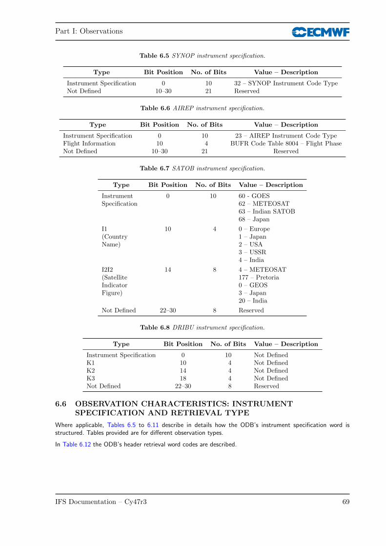
Part I: Observations
Table 6.5 SYNOP instrument specification.
Type Bit Position No. of Bits Value – Description
Instrument Specification 0 10 32 – SYNOP Instrument Code TypeNot Defined 10–30 21 Reserved
Table 6.6 AIREP instrument specification.
Type Bit Position No. of Bits Value – Description
Instrument Specification 0 10 23 – AIREP Instrument Code TypeFlight Information 10 4 BUFR Code Table 8004 – Flight PhaseNot Defined 10–30 21 Reserved
Table 6.7 SATOB instrument specification.
Type Bit Position No. of Bits Value – Description
InstrumentSpecification
0 10 60 - GOES62 – METEOSAT63 – Indian SATOB68 – Japan
I1(CountryName)
10 4 0 – Europe1 – Japan2 – USA3 – USSR4 – India
I2I2(SatelliteIndicatorFigure)
14 8 4 – METEOSAT177 – Pretoria0 – GEOS3 – Japan20 – India
Not Defined 22–30 8 Reserved
Table 6.8 DRIBU instrument specification.
Type Bit Position No. of Bits Value – Description
Instrument Specification 0 10 Not DefinedK1 10 4 Not DefinedK2 14 4 Not DefinedK3 18 4 Not DefinedNot Defined 22–30 8 Reserved
6.6 OBSERVATION CHARACTERISTICS: INSTRUMENTSPECIFICATION AND RETRIEVAL TYPE
Where applicable, Tables 6.5 to 6.11 describe in details how the ODB’s instrument specification word isstructured. Tables provided are for different observation types.
In Table 6.12 the ODB’s header retrieval word codes are described.
IFS Documentation – Cy47r3 69
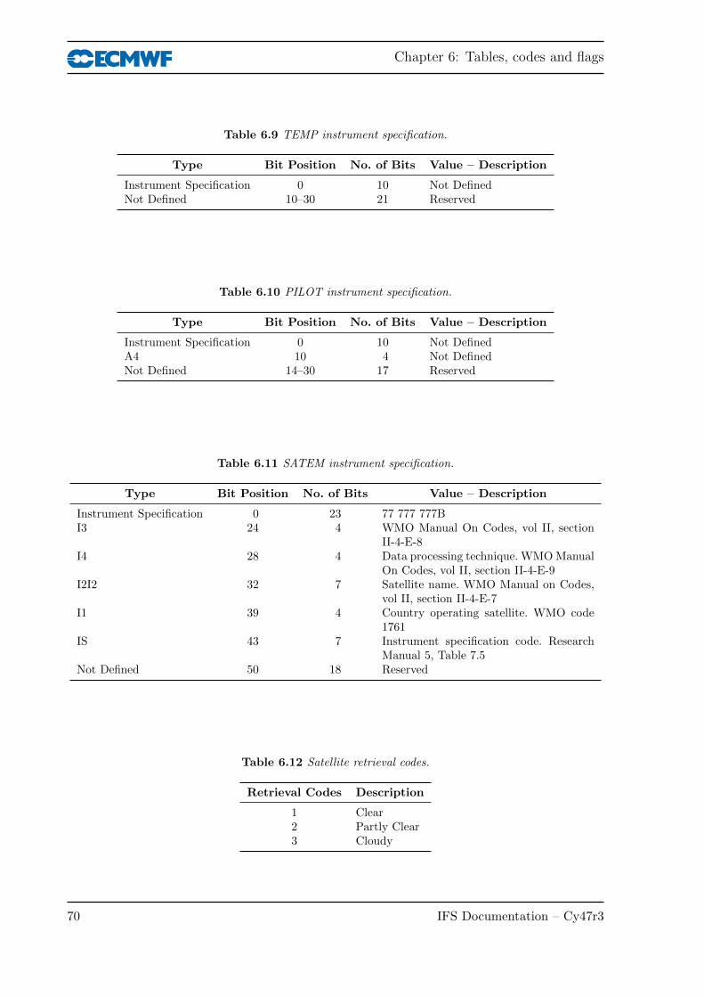
Chapter 6: Tables, codes and flags
Table 6.9 TEMP instrument specification.
Type Bit Position No. of Bits Value – Description
Instrument Specification 0 10 Not DefinedNot Defined 10–30 21 Reserved
Table 6.10 PILOT instrument specification.
Type Bit Position No. of Bits Value – Description
Instrument Specification 0 10 Not DefinedA4 10 4 Not DefinedNot Defined 14–30 17 Reserved
Table 6.11 SATEM instrument specification.
Type Bit Position No. of Bits Value – Description
Instrument Specification 0 23 77 777 777BI3 24 4 WMO Manual On Codes, vol II, section
II-4-E-8I4 28 4 Data processing technique. WMOManual
On Codes, vol II, section II-4-E-9I2I2 32 7 Satellite name. WMO Manual on Codes,
vol II, section II-4-E-7I1 39 4 Country operating satellite. WMO code
1761IS 43 7 Instrument specification code. Research
Manual 5, Table 7.5Not Defined 50 18 Reserved
Table 6.12 Satellite retrieval codes.
Retrieval Codes Description
1 Clear2 Partly Clear3 Cloudy
70 IFS Documentation – Cy47r3

Part I: Observations
Table 6.13 Vertical coordinate.
Vertical Coordinate Codes Description
1 Pressure (Pa)2 Height (GPM)3 Satellite Channel (numeric)4 Scatterometer Channel (numeric)
Table 6.14 Pressure codes.
Pressure Codes Description
0 Sea Level1 Station Level2 850 hPa Geopotential3 700 hPa Geopotential4 500 hPa Geopotential5 1000 GPM Pressure6 2000 GPM Pressure7 3000 GPM Pressure8 4000 GPM Pressure9 900 hPa Geopotential
10 1000 hPa Geopotential11 500 hPa Geopotential12 925 hPa Geopotential
Table 6.15 Level ID.
Bit Position No. of Bits Value – Description
0 1 1 – Max Wind Level1 1 1 – Tropopause2 1 1 – D Part3 1 1 – C Part4 1 1 – B Part5 1 1 – A Part6 1 1 – Surface Level7 1 1 – Significant Wind Level8 1 1 – Significant Temperature Level
9–31 24 Not Defined
6.7 VERTICAL COORDINATE: PRESSURE, SATELLITE ID ANDLEVEL ID CODES
In the ODB the vertical coordinate is expressed by various codes, and Table 6.13 describes those codes.
Also, the ODB pressure code word is expressed in terms of codes which are defined in Table 6.14.
Upper air observations (TEMP and PILOT) have the level at which the observation was taken defined in termswhat it is and that information is stored in the ODB. Details are given in Table 6.15.
IFS Documentation – Cy47r3 71
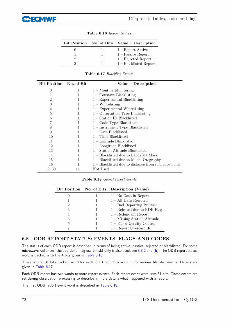
Chapter 6: Tables, codes and flags
Table 6.16 Report Status.
Bit Position No. of Bits Value – Description
0 1 1 – Report Active1 1 1 – Passive Report2 1 1 – Rejected Report3 1 1 – Blacklisted Report
Table 6.17 Blacklist Events.
Bit Position No. of Bits Value – Description
0 1 1 – Monthly Monitoring1 1 1 – Constant Blacklisting2 1 1 – Experimental Blacklisting3 1 1 – Whitelisting4 1 1 – Experimental Whitelisting5 1 1 – Observation Type Blacklisting6 1 1 – Station ID Blacklisted7 1 1 – Code Type Blacklisted8 1 1 – Instrument Type Blacklisted9 1 1 – Date Blacklisted10 1 1 – Time Blacklisted11 1 1 – Latitude Blacklisted12 1 1 – Longitude Blacklisted13 1 1 – Station Altitude Blacklisted14 1 1 – Blacklisted due to Land/Sea Mask15 1 1 – Blacklisted due to Model Orography16 1 1 – Blacklisted due to distance from reference point
17–30 14 Not Used
Table 6.18 Global report events.
Bit Position No. of Bits Description (Value)
0 1 1 – No Data in Report1 1 1 – All Data Rejected2 1 1 – Bad Reporting Practice3 1 1 – Rejected due to RDB Flag4 1 1 – Redundant Report5 1 1 – Missing Station Altitude6 1 1 – Failed Quality Control7 1 1 – Report Overcast IR
6.8 ODB REPORT STATUS: EVENTS, FLAGS AND CODES
The status of each ODB report is described in terms of being active, passive, rejected or blacklisted. For somemicrowave radiances, the additional flag use emiskf only is also used, see 3.3.2 and (b). The ODB report statusword is packed with the 4 bits given in Table 6.16.
There is one, 31 bits packed, word for each ODB report to account for various blacklist events. Details aregiven in Table 6.17.
Each ODB report has two words to store report events. Each report event word uses 31 bits. These events areset during observation processing to describe in more details what happened with a report.
The first ODB report event word is described in Table 6.18.
72 IFS Documentation – Cy47r3

Part I: Observations
Table 6.19 TEMP report events.
Bit Position No. of Bits Value – Description
0 1 1 - Old Style Z Bias Correction Applied1 1 1 - New Style T Bias Correction Applied2 1 1 - RH Bias Correction Applied
3–30 28 Not Used
Table 6.20 PILOT report events.
Bit Position No. of Bits Value – Description
0 1 1 - American Wind Profiler1 1 1 - European Wind Profiler
2–30 29 Not Used
Table 6.21 SATEM report events.
Bit Position No. of Bits Value – Description
0 1 1 - Thinned Report1–30 30 Not Used
Table 6.22 SCAT report events.
Bit Position No. of Bits Value – Description
0 1 1 - Report thinned in across-node direction1 1 1 - Reported Wind Directions too Close2 1 1 - Report in QuikScat outer swath3 1 1 - Report Contaminated by Rain
4–30 29 Not Used
The second ODB report event word holds an additional set of events which are now dependent on observationtype. Details are given in Tables 6.19 to 6.22.
The ODB report RDB flag word ([DEPRECATED], probably unused) is 30 bits packed which contains flagsfor five report parameters: latitude, longitude, date, time and altitude. Each parameter occupies 6 bits withfurther stratification which is identical for every parameter as indicated in Table 6.23.
IFS Documentation – Cy47r3 73

Chapter 6: Tables, codes and flags
Table 6.23 RDB report (latitude, longitude, date, time and altitude) flags. [DEPRECATED], probablyunused.
No. of BitParameter Bits Position
Bit No. ofPosition Bits Value – Description
0 1 0 – No Human Monitoring Substitution1 – Human Monitoring Substitution
Latitude 6 0+ +1 1 0 – No Q/C SubstitutionLongitude 6 6+ 1 – Q/C SubstitutionDate 6 12+ +2 1 0 – Override Flag not SetTime 6 18+ 1 – Override Flag SetAltitude 6 24+ +3 2 0 – Parameter Correct
1 – Parameter Probably Correct2 – Parameter Probably Incorrect3 – Parameter Incorrect
+5 1 0 – Parameter Flag Set by Q/C or not Checked1 – Parameter Flag Set by Human Monitoring
74 IFS Documentation – Cy47r3

Part I: Observations
Table 6.24 Datum status.
Bit Position No. of Bits Value – Description
0 1 1 – Report Active1 1 1 – Passive Report2 1 1 – Rejected Report3 1 1 – Blacklisted Report
Table 6.25 Global datum events.
Bit Position No. of Bits Value – Description
0 1 1 – Missing Vertical Coordinate1 1 1 – Missing Observed Value2 1 1 – Missing Background (First Guess) Value3 1 1 – Rejected due to RDB Flag4 1 1 – Activated due to RDB Flag5 1 1 – Activated by Whitelist6 1 1 – Bad Reporting Practice7 1 1 – Vertical Position out of Range8 1 1 – Reference Level Position out of Range9 1 1 – Too Big First Guess Departure10 1 1 – Too Big Departure in Assimilation11 1 1 – Too Big Observation Error12 1 1 – Redundant Datum13 1 1 – Redundant Level14 1 1 – Report Over Land15 1 1 – Report Over Sea16 1 1 – Not Analysis Variable17 1 1 – Duplicate Datum/Level18 1 1 – Too Many Surface Data19 1 1 – Multi Level Check20 1 1 – Level Selection21 1 1 – Vertical Consistency Check22 1 1 – Vertical Coordinate Changed from Z to P23 1 1 – Datum Rejected via Namelist24 1 1 – Combined Flagging25 1 1 – Datum Rejected due to Rejected Report26 1 1 – Variational QC Performed27 1 1 – Observation Error Increased28 1 1 – Cloud Contamination29 1 1 – Rain Contamination30 1 1 – Aerosol Contamination31 1 1 – Missing or Not Sensible Emissivity Values
6.9 DATUM STATUS: EVENTS, RDB AND ANALYSIS FLAGS
The status of each datum, like report status, is described in terms of being: active, passive, rejected orblacklisted. Table 6.24 shows that the ODB datum status is a packed word with 4 bits used to describe itsstatus.
There are two ODB words reserved for datum events. They both use 31 bits each to store relevant information.The first event word has the same structure for all observation types, whereas the second event word isobservation type dependent. Tables 6.25 to 6.28 describe the event words structures for the observation typesthat use them.
IFS Documentation – Cy47r3 75
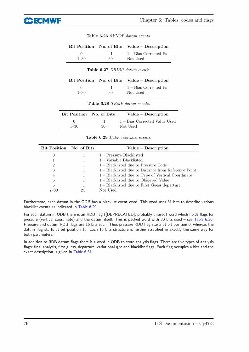
Chapter 6: Tables, codes and flags
Table 6.26 SYNOP datum events.
Bit Position No. of Bits Value – Description
0 1 1 – Bias Corrected Ps1–30 30 Not Used
Table 6.27 DRIBU datum events.
Bit Position No. of Bits Value – Description
0 1 1 – Bias Corrected Ps1–30 30 Not Used
Table 6.28 TEMP datum events.
Bit Position No. of Bits Value – Description
0 1 1 – Bias Corrected Value Used1–30 30 Not Used
Table 6.29 Datum blacklist events.
Bit Position No. of Bits Value – Description
0 1 1 – Pressure Blacklisted1 1 1 – Variable Blacklisted2 1 1 – Blacklisted due to Pressure Code3 1 1 – Blacklisted due to Distance from Reference Point4 1 1 – Blacklisted due to Type of Vertical Coordinate5 1 1 – Blacklisted due to Observed Value6 1 1 – Blacklisted due to First Guess departure
7–30 24 Not Used
Furthermore, each datum in the ODB has a blacklist event word. This word uses 31 bits to describe variousblacklist events as indicated in Table 6.29.
For each datum in ODB there is an RDB flag ([DEPRECATED], probably unused) word which holds flags forpressure (vertical coordinate) and the datum itself. This is packed word with 30 bits used – see Table 6.30.Pressure and datum RDB flags use 15 bits each. Thus pressure RDB flag starts at bit position 0, whereas thedatum flag starts at bit position 15. Each 15 bits structure is further stratified in exactly the same way forboth parameters:
In addition to RDB datum flags there is a word in ODB to store analysis flags. There are five types of analysisflags: final analysis, first guess, departure, variational q/c and blacklist flags. Each flag occupies 4 bits and theexact description is given in Table 6.31.
76 IFS Documentation – Cy47r3

Part I: Observations
Table 6.30 RDB pressure (vertical coordinate) and datum flags. [DEPRECATED], probably unused.
No. of BitParameter Bits Position
Bit No. ofPosition Bits Value – Description
0 1 0 – No Human MonitoringSubstitution1 – Human MonitoringSubstitution
+1 1 0 – No Q/C SubstitutionPressure 15 0+ 1 – Q/C SubstitutionDatum 15 15+ +2 1 0 – Override Flag not Set
1 – Override Flag Set+3 2 0 – Correct
1 – Probably Correct2 – Probably Incorrect3 – Parameter Incorrect
+5 1 0 – Flag Set by Q/C or notChecked1 – Flag Set by HumanMonitoring
+6 2 0 – Previous Analysis judged itcorrect1 – Previous Analysis judged itprobably correct2 – Previous Analysis judged itprobably incorrect3 – Previous Analysis judged itincorrect
+8 1 0 – Not used by previousanalysis1 – Used by previous analysis
+9 5 Not Used
IFS Documentation – Cy47r3 77

Chapter 6: Tables, codes and flags
Table 6.31 Analysis flags. DEPRECATED, probably unused.
Flag Type Bit Position No. of Bits Value – Description
Final 0 4 0 – Correct1 – Probably correct2 – Probably incorrect
3 – Incorrect
First Guess 4 4 0 – Correct1 – Probably correct2 – Probably incorrect
3 – Incorrect
Departure 8 4 0 – Correct1 – Probably correct2 – Probably incorrect
3 – Incorrect
Variational Q/C 12 4 0 – Correct1 – Probably correct2 – Probably incorrect
3 – Incorrect
Blacklist 16 4 0 – Correct1 – Probably correct2 – Probably incorrect
3 – Incorrect
Not Defined 20 11 Reserved
78 IFS Documentation – Cy47r3

Part I: Observations
References
Alduchov, O. A. and Eskridge, R. E. (1996). Improved Magnus form approximation of saturation vaporpressure. J. Appl. Meteorol., 35, 601–609.
Andersson, E., Pailleux, J., Thepaut, J.-N., Eyre, J. R., McNally, A. P., Kelly, G. A. and Courtier, P. (1994).Use of cloud-cleared radiances in three/four-dimensional variational data assimilation. Q. J. R. Meteorol.Soc., 120, 627–653.
Baordo, F. and Geer, A. J. (2016). Assimilation of SSMIS humidity-sounding channels in all-sky conditionsover land using a dynamic emissivity retrieval. Quarterly Journal of the Royal Meteorological Society, doi:10.1002/qj.2873.
Bauer, P., Geer, A. J., Lopez, P. and Salmond, D. (2010). Direct 4D-Var assimilation of all-sky radiances:Part I. Implementation. Q. J. R. Meteorol. Soc., 136, 1868–1885.
Blondin, C. (1991). Parametrization of land surface processes in numerical weather prediction. In T. J.Schmugge and J.-C. Andre (Eds), Land Surface Evaporation: Measurement and Parametrization, pp. 31–54,Springer-Verlag.
Bonavita, M., Dahoui, M., Lopez, P., Prates, F., Holm, E., Chiara, G. D., Geer, A., Isaksen, L. and Ingleby,B. (2017). On the initialization of tropical cyclones. ECMWF Tech. Memo. No. 810.
Bormann, N. (2014). Reformulation of the emissivity kalman filter atlas. RD Internal Memorandum, p. 14pp,available online: http://intra.ecmwf.int/publications/library/do/references/show?id=1471.
Bormann, N. (2017). Slant path radiative transfer for the assimilation of sounder radiances. Tellus A: DynamicMeteorology and Oceanography, 69(1), 1272779.
Bormann, N. and Bonavita, M. (2013). Spread of the ensemble of data assimilations in radiance space.ECMWF Technical Memorandum 708.
Bormann, N., Bonavita, M., Dragani, R., Eresmaa, R., Matricardi, M. and McNally, A. (2016). Enhancingthe impact of IASI observations through an updated observation-error covariance matrix. Q. J. R. Meteorol.Soc., 142, 1767–1780.
Bormann, N. and Healy, S. (2006). A fast radiative-transfer model for the assimilation of MIPAS limbradiances: Accounting for horizontal gradients. Q. J. R. Meteorol. Soc., 132, 2357–2376.
Bormann, N., Healy, S. and Hamrud, M. (2007). Assimilation of MIPAS limb radiances in the ECMWF system.Part II: Experiments with a 2-dimensional observation operator and comparison to retrieval assimilation.Q. J. R. Meteorol. Soc., 133, 329–346.
Bormann, N., Matricardi, M. and Healy, S. (2005). A fast radiative transfer model for the assimilation ofinfrared limb radiances from MIPAS. Q. J. R. Meteorol. Soc., 131, 1631–1653.
Bormann, N., Saarinen, S., Kelly, G. and Thepaut, J.-N. (2003). The spatial structure of observation errorsin atmospheric motion vectors from geostationary satellite data. Mon. Wea. Rev., 131, 706–718.
Bormann, N. and Thepaut, J.-N. (2007). Assimilation of MIPAS limb radiances in the ECMWF system. PartI: Experiments with a 1-dimensional observation operator. Q. J. R. Meteorol. Soc., 133, 309–327.
IFS Documentation – Cy47r3 79

References
Buck, A. L. (1981). New equations for computing vapor pressure and enhancement factor. J. Appl. Meteorol.,20, 1527–1532.
Cardinali, C., Andersson, E., Viterbo, P., Thepaut, J.-N. and Vasiljevic, D. (1994). Use of conventional surfaceobservations in three-dimensional variational data assimilation. ECMWF Tech. Memo. No. 205.
Cardinali, C., Isaksen, L. and Andersson, E. (2003). Use and impact of automated aircraft data in a global4D-Var data assimilation system. Mon. Wea. Rev., 131, 1865–1877.
Courtier, P., Andersson, E., Heckley, W., Pailleux, J., Vasiljevic, D., Hamrud, M., Hollingsworth, A., Rabier, F.and Fisher, M. (1998). The ECMWF implementation of three dimensional variational assimilation (3D-Var).I: Formulation. Q. J. R. Meteorol. Soc., 124, 1783–1807.
Deblonde, G. and English, S. (2001). Evaluation of the fastem-2 fast microwave oceanic surface emissivitymodel. In Tech. Proc. ITSC-XI, pp. 67–78, Budapest.
Engelen, R. J., Andersson, E., Chevallier, F., Hollingsworth, A., Matricardi, M., McNally, A., Thepaut, J.-N.and Watts, P. (2004). Estimating atmospheric CO2 from advanced infrared satellite radiances within anoperational 4D-Var data assimilation system: Methodology and first results. J. Geophys. Res., 109, D19309.
Eyre, J. R. (1991). A fast radiative transfer model for satellite sounding systems. ECMWF Tech. Memo.No. 176.
Geer, A. J., Baordo, F., Bormann, N. and English, S. (2014). All-sky assimilation of microwave humiditysounders. ECMWF technical memorandum, in preparation.
Geer, A. J. and Bauer, P. (2011). Observation errors in all-sky data assimilation. Q. J. R. Meteorol. Soc.,DOI: 10.1002/qj.830.
Geer, A. J. and Bauer, P. (2012). Assimilating AMSU-A radiances sensitive to cloud and temperature usingthe all-sky approach. ECMWF technical memorandum 670.
Geer, A. J., Bauer, P. and Lopez, P. (2008). Lessons learnt from the operational 1D+4D-Var assimilation ofrain- and cloud-affected SSM/I observations at ECMWF. Q. J. R. Meteorol. Soc., 134, 1513–1525.
Geer, A. J., Bauer, P. and Lopez, P. (2010). Direct 4D-Var assimilation of all-sky radiances: Part II.Assessment. Q. J. R. Meteorol. Soc., 136, 1886–1905.
Geleyn, J.-F. (1988). Interpolation of wind, temperature and humidity values from the model levels to theheight of meaurement. Tellus, 40, 347–351.
Han, W. and Bormann, N. (2016). Constrained adaptive bias correction for satellite radiance assimilation inthe ECMWF 4D-Var system. ECMWF Tech. Memo. No. 783., doi:10.21957/rex0omex.
Healy, S. and Thepaut, J.-N. (2006). Assimilation experiments with CHAMP GPS radio occultationmeasurements. Q. J. R. Meteorol. Soc., 132, 605–623.
Hersbach, H. (2010a). Assimilation of scatterometer data as equivalent-neutral wind. ECMWF Tech. Memo.No. 629.
Hersbach, H. (2010b). Comparison of c-band scatterometer cmod5.n equivalent neutral winds with ecmwf.J. Atmos. Oceanic Technol., 27, 721–736.
Hersbach, H. (2011). Sea surface roughness and drag coefficient as functions of neutral wind speed. J. Phys.Oceanogr., 41, 247–251.
Hersbach, H., Stoffelen, A. and de, S. H. (2007). An improved C-band scatterometer ocean geophysical modelfunction: CMOD5. J. Geophys. Res., 112, doi:10.1029/2006JC003743.
Hocking, J. (2014). Interpolation methods in the rttov radiative transfer model. Forecast Research TechnicalReport No. 590.
80 IFS Documentation – Cy47r3
Part I: Observations
Huddleston, J. N. and Stiles, B. W. (2000). Multidimensional histogram (MUDH) rain flag. ProductDescription Version 2.1, URL http://podaac-www.jpl.nasa.gov/quikscat/.
Ingleby, B. (2015). Global assimilation of air temperature, humidity, wind and pressure from surface stations.Q. J. R. Meteorol. Soc., 141, 504–517.
Isaksen, L. and Janssen, P. A. E. M. (2004). Impact of ERS scatterometer winds in ECMWF’s assimilation.Q. J. R. Meteorol. Soc., 130, 1793–1814.
Jarvinen, H., Andersson, E. and Bouttier, F. (1999). Variational assimilation of time sequences of surfaceobservations with serially correlated errors. ECMWF Tech. Memo. No. 266.
Jarvinen, H., Saarinen, S. and Unden, P. (1996). User’s Guide for Blacklisting. Available on request fromECMWF, Shinfield Park, RG2 9AX, Reading, Berkshire, UK.
Jarvinen, H. and Unden, P. (1997). Observation screening and first guess quality control in the ECMWF3D-Var data assimilation system. ECMWF Tech. Memo. No. 236.
Karbou, F., Gerard, E. and Rabier, F. (2006). Microwave land emissivity and skin temperature for AMSU-Aand -B assimilation over land. Q. J. R. Meteorol. Soc., 132, 2333–2355.
Krzeminski, B., Bormann, N., Karbou, F. and Bauer, P. (2009a). Improved use of surface-sensitive microwaveradiances at ECMWF. In Proceedings of 2009 EUMETSAT Meteorological Satellite Conference, Bath, UnitedKingdom.
Krzeminski, B., Bormann, N., Kelly, G., McNally, A. and Bauer, P. (2009b). Revision of the HIRS clouddetection at ecmwf. ECMWF/EUMETSAT fellowship reports No. 19.
Lean, K. and Bormann, N. (2021). Using model cloud information to reassign low level AMVs for NWP.ECMWF/EUMETSAT fellowship reports No. 56.
Lean, P., Geer, A., Salmond, D. and Hague, J. (2016). The cost and scalability of observation processing inIFS; implications for future observation usage. RD internal memo, RD16-045.
Leidner, S. M., Hoffman, R. N. and Augenbaum, J. (2000). SeaWinds Scatterometer Real-Time BUFRGeophysical Data Product, User’s Guide Version 2.3.0. NOAA/NESDIS.
Lonnberg, P. (1989). Developments in the ECMWF analysis system. In Proc. ECMWF Seminar on Dataassimilation and the Use of Satellite Data, pp. 75–119, Reading, 5–9 September 1988.
Lonnberg, P. and Shaw, D. (1985). Data selection and quality control in the ECMWF analysis system. InECMWF Workshop on The Use And Quality Control of Meteorological Observations, pp. 225–254, Reading,6–9 November 1984.
Lonnberg, P. and Shaw, D. (Eds) (1987). ECMWF Data Assimilation Scientific Documentation, ResearchManual 1.
Lopez, P. (2011). Direct 4d-var assimilation of NCEP stage IV radar and gauge precipitation data at ecmwf.Monthly Weather Review, 139(7), 2098–2116.
Lorenc, A. C. (1986). Analysis methods for numerical weather prediction. Q. J. R. Meteorol. Soc., 112,1177–1194.
Louis, J.-F. (1979). A parametric model of vertical eddy fluxes in the atmosphere. Boundary-Layer Meteorol.,17, 187–202.
Louis, J.-F., Tiedtke, M. and Geleyn, J.-F. (1982). A short history of the PBL parametrization at ECMWF.In Proc. ECMWF Workshop on Planetary Boundary Layer Parameterization, pp. 59–80, Reading, 25–27November, 1981.
Lupu, C. and McNally, A. (2012). Assimilation of cloud affected radiances from meteosat-9 at ecmwf.ECMWF/EUMETSAT fellowship reports No. 25.
IFS Documentation – Cy47r3 81

References
Matricardi, M., Chevallier, F. and Tjemkes, S. (2001). An improved fast radiative transfer model for theassimilation of radiance observations. ECMWF Tech. Memo. No. 345.
McNally, A. P. (2009). The direct assimilation of cloud affected satellite infrared radiances in the ecmwf4d-var. Q. J. R. Meteorol. Soc., 135, 1214–1229.
McNally, A. P., Andersson, E., Kelly, G. and Saunders, R. W. (1999). The use of raw TOVS/ATOVS radiancesin the ECMWF 4D-Var assimilation system. ECMWF Newsletter No. 83, pp. 2–7.
McNally, A. P. and Watts, P. D. (2003). A cloud detection algorithm for high spectral resolution infraredsounders. Q. J. R. Meteorol. Soc., 129, 3411–3423.
Munro, R., Kopken, C., Kelly, G., Thepaut, J.-N. and Saunders, R. (2004). Assimilation of Meteosatradiance data within the 4D-Var system at ECMWF: Data quality monitoring, bias correction and single-cycleexperiments. Q. J. R. Meteorol. Soc., 130, 2293–2313.
Pailleux, J. (1990). A global variational assimilation scheme and its application for using TOVS radiances.In Proc. WMO International Symposium on Assimilation of Observations in Meteorology and Oceanography,pp. 325–328, Clermont-Ferrand, France.
Saunders, R. W. and Matricardi, M. (1998). A fast forward model for ATOVS (RTATOV). In Tech. Proc.9th International TOVS Study Conference, p. 11 pp, Igls, Austria, 20–26 February, 1997.
Sherlock, V. J. (1999). ISEM-6: Infrared Surface Emissivity Model for RRTOV-6. Forecasting ResearchTechnical Report No. 299, available from Met Office, London Road, Bracknell, Berkshire RG12 2SZ, UK.
Simmons, A. J. and Burridge, D. (1981). An energy and angular momentum conserving vertical finitedifference scheme and hybrid coordinate. Mon. Wea. Rev., 109, 758–766.
Simmons, A. J. and Chen, J. (1991). The calculation of geopotential and the pressure gradient in the ECMWFatmospheric model: Influence on the simulation of the polar atmosphere and on temperature analyses. Q. J. R.Meteorol. Soc., 117, 29–58.
Stoffelen, A. and Anderson, D. (1997). Ambiguity removal and assimilation of scatterometer data. Q. J. R.Meteorol. Soc., 123, 491–518.
Tomassini, M., LeMeur, D. and Saunders, R. W. (1998). Near-surface satellite wind observations of hurricanesand their impact on ECMWF model analyses and forecasts. Mon. Wea. Rev., 126, 1274–1286.
Vasiljevic, D., Cardinali, C. and Unden, P. (1992). ECMWF 3D-Variational assimilation of conventionalobservations. In Proc. ECMWF Workshop on Variational Assimilation with Emphasis on Three-dimensionalAspects, Reading, 9–12 November 1992.
Wattrelot, E., Caumont, O. and Mahfouf, J.-F. (2014). Operational implementation of the 1D+3D-Varassimilation method of radar reflectivity data in the AROME model. Monthly Weather Review, 142(5),1852–1873.
82 IFS Documentation – Cy47r3