part ii: how to make a bayesian model. questions you can answer… what would an ideal learner or...
Post on 22-Dec-2015
218 views
TRANSCRIPT
Part II: How to make a Bayesian model
Questions you can answer…
• What would an ideal learner or observer infer from these data?
• What are the effects of different assumptions or prior knowledge on this inference?
• What kind of constraints on learning are necessary to explain the inferences people make?
• How do people learn a structured representation?

Marr’s three levels
Computation “What is the goal of the computation, why is it
appropriate, and what is the logic of the strategy by which it can be carried out?”
Representation and algorithm “What is the representation for the input and output,
and the algorithm for the transformation?”
Implementation “How can the representation and algorithm be realized
physically?”
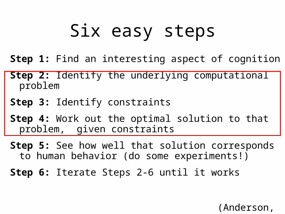
Six easy steps
Step 1: Find an interesting aspect of cognition
Step 2: Identify the underlying computational problem
Step 3: Identify constraints
Step 4: Work out the optimal solution to that problem, given constraints
Step 5: See how well that solution corresponds to human behavior (do some experiments!)
Step 6: Iterate Steps 2-6 until it works
(Anderson, 1990)
A schema for inductive problems
• What are the data?– what information are people learning or drawing
inferences from?
• What are the hypotheses?– what kind of structure is being learned or inferred
from these data?
(these questions are shared with other models)
Thinking generatively…• How do the hypotheses generate the data?
– defines the likelihood p(d|h)
• How are the hypotheses generated?– defines the prior p(h)– while the prior encodes information about knowledge
and learning biases, translating this into a probability distribution can be made easier by thinking in terms of a generative process…
• Bayesian inference inverts this generative process
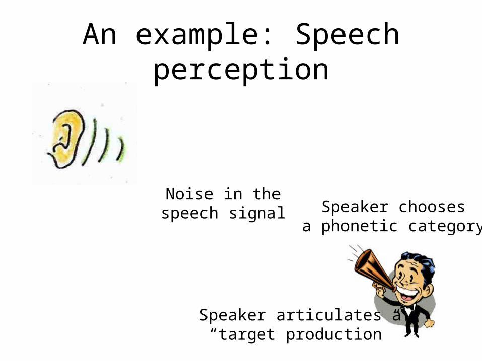
An example: Speech perception
(with thanks to Naomi Feldman )
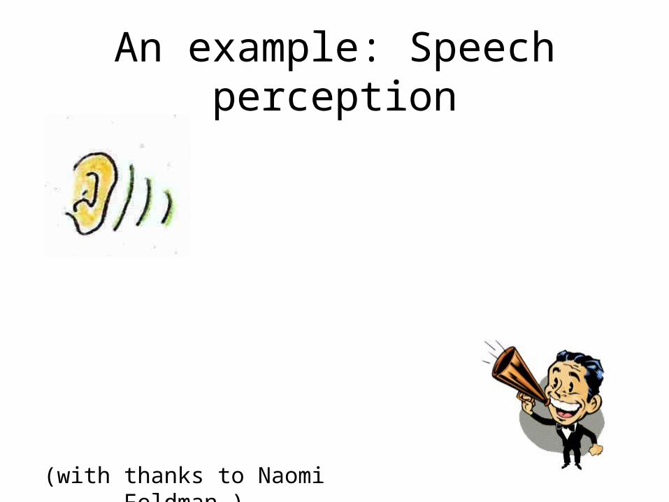
An example: Speech perception
Speaker choosesa phonetic category
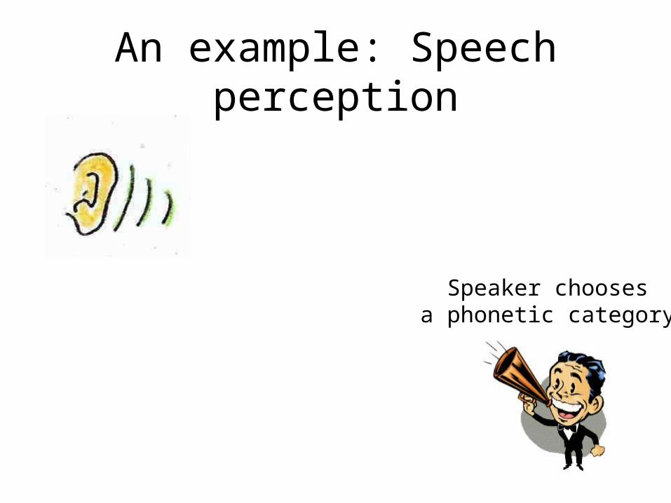
An example: Speech perception
Speaker choosesa phonetic category
Speaker articulates a“target production”
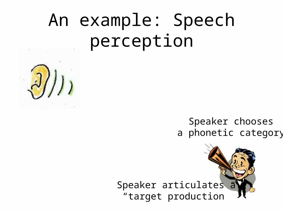
An example: Speech perception
Speaker choosesa phonetic category
Noise in thespeech signal
Speaker articulates a“target production”

An example: Speech perceptionListener hearsa speech sound
Speaker choosesa phonetic category
Noise in thespeech signal
Speaker articulates a“target production”

An example: Speech perceptionListener hearsa speech sound
Speaker choosesa phonetic category
Noise in thespeech signal
cS
TSpeaker articulates a“target production”
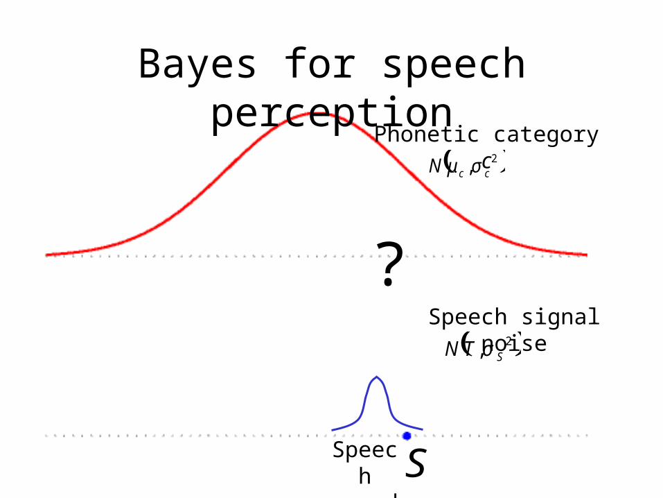
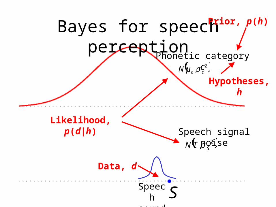
Bayes for speech perception
?
( )2, ccN σμ
Phonetic category c
SSpeech sound
( )2, STN σ
Speech signal noise
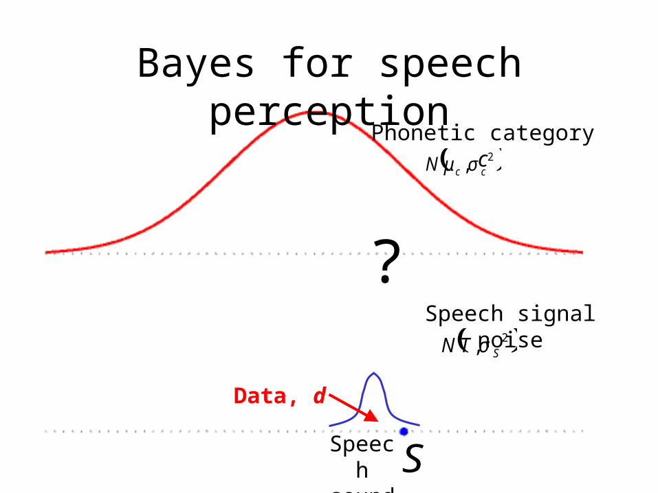
Bayes for speech perception
?
( )2, ccN σμ
Phonetic category c
Speech sound
( )2, STN σ
Speech signal noise
Data, d
S

Bayes for speech perception
?
( )2, ccN σμ
Phonetic category c
Speech sound
( )2, STN σ
Speech signal noiseHypotheses, h
Data, d
S

Bayes for speech perception
?
( )2, ccN σμ
Phonetic category c
Speech sound
( )2, STN σ
Speech signal noise
Prior, p(h)
Hypotheses, h
Data, d
S
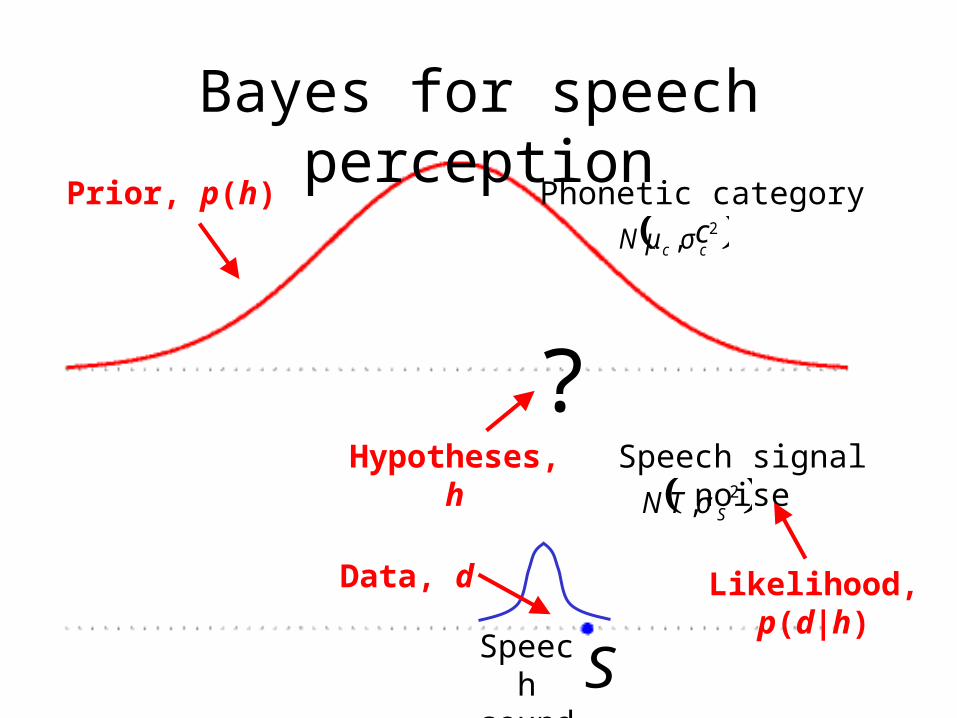
Bayes for speech perception
?
( )2, ccN σμ
Phonetic category c
Speech sound
( )2, STN σ
Speech signal noise
Prior, p(h)
Hypotheses, h
Data, d Likelihood, p(d|h)
S

Bayes for speech perception
Listeners must invert the process that generated the sound they heard…
– data (d): speech sound S– hypotheses (h): target productions T– prior (p(h)): phonetic category structure p(T|c)
– likelihood (p(d|h)): speech signal noise p(S|T) ( ) ( ) ( )hphdpdhp || ∝
Bayes for speech perception
( )2, ccN σμ
Phonetic category c
Speech sound
( )2, STN σ
Speech signal noise
Prior, p(h)
Hypotheses, h
Data, d
Likelihood, p(d|h)
S
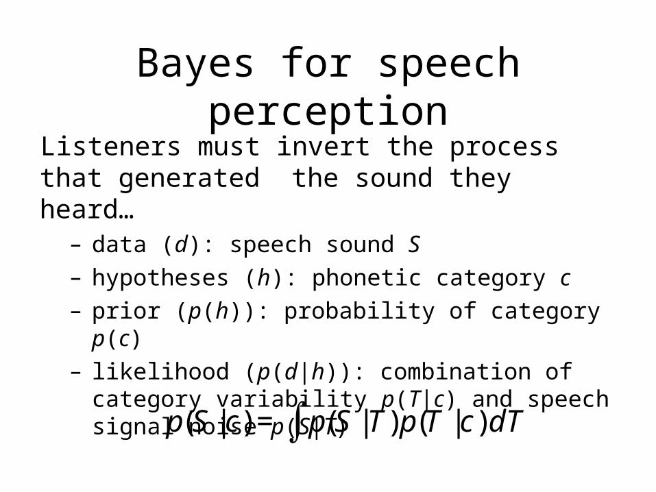
Bayes for speech perception
Listeners must invert the process that generated the sound they heard…
– data (d): speech sound S– hypotheses (h): phonetic category c– prior (p(h)): probability of category p(c)– likelihood (p(d|h)): combination of category
variability p(T|c) and speech signal noise p(S|T)
€
p(S | c) = p(S | T)p(T | c) dT∫
Challenges of generative models
• Specifying well-defined probabilistic models involving many variables is hard
• Representing probability distributions over those variables is hard, since distributions need to describe all possible states of the variables
• Performing Bayesian inference using those distributions is hard

Graphical models
• Express the probabilistic dependency structure among a set of variables (Pearl, 1988)
• Consist of– a set of nodes, corresponding to variables– a set of edges, indicating dependency– a set of functions defined on the graph that
specify a probability distribution
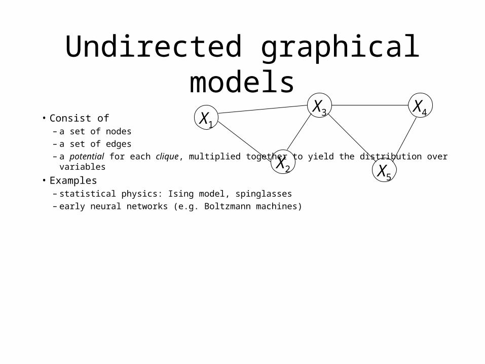
Undirected graphical models
• Consist of– a set of nodes– a set of edges– a potential for each clique, multiplied together to yield the distribution over variables
• Examples– statistical physics: Ising model, spinglasses– early neural networks (e.g. Boltzmann machines)
X1
X2
X3 X4
X5
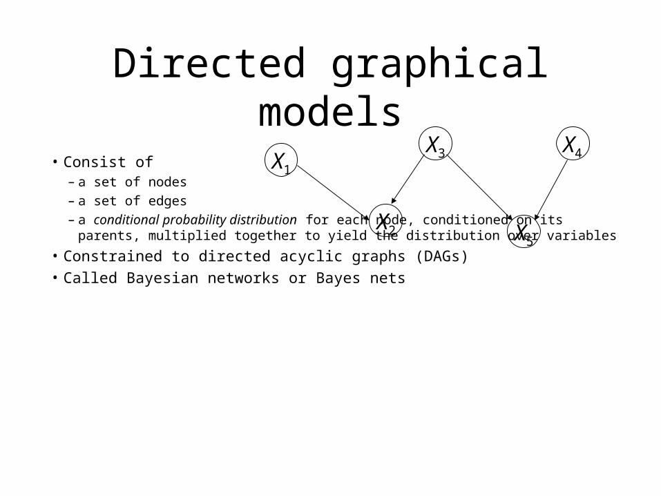
Directed graphical modelsX3 X4
X5
X1
X2
• Consist of– a set of nodes– a set of edges– a conditional probability distribution for each node, conditioned on its parents, multiplied together
to yield the distribution over variables
• Constrained to directed acyclic graphs (DAGs)• Called Bayesian networks or Bayes nets
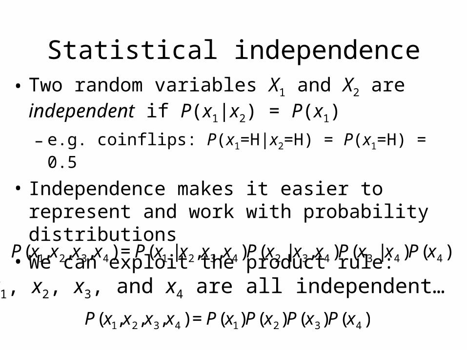
Statistical independence• Two random variables X1 and X2 are independent if
P(x1|x2) = P(x1)
– e.g. coinflips: P(x1=H|x2=H) = P(x1=H) = 0.5
• Independence makes it easier to represent and work with probability distributions
• We can exploit the product rule:
€
P(x1,x2, x3, x4 ) = P(x1 | x2,x3,x4 )P(x2 | x3, x4 )P(x3 | x4 )P(x4 )
€
P(x1, x2, x3, x4 ) = P(x1)P(x2)P(x3)P(x4 )
If x1, x2, x3, and x4 are all independent…
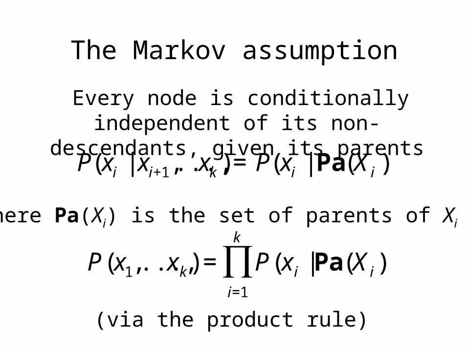
The Markov assumption
Every node is conditionally independent of its non-descendants, given its parents
€
P(xi | xi+1,...,xk ) = P(xi | Pa(X i ))
where Pa(Xi) is the set of parents of Xi
€
P(x1,..., xk ) = P(x i | Pa(X i))i=1
k
∏
(via the product rule)
Representing generative models
• Graphical models provide solutions to many of the challenges of probabilistic models– defining structured distributions– representing distributions on many variables– efficiently computing probabilities
• Graphical models also provide an intuitive way to define generative processes…

Graphical model for speech
c Choose a category c with probability p(c)
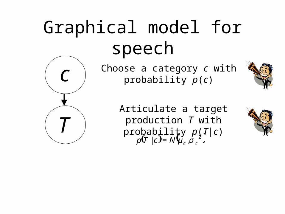
Graphical model for speech
( ) ( )2,| ccNcTp σμ=
c Choose a category c with probability p(c)
Articulate a target production T with probability p(T|c)T

Graphical model for speech
( ) ( )2,| ccNcTp σμ=
c
S
Choose a category c with probability p(c)
Articulate a target production T with probability p(T|c)
Listener hears speech sound S with probability p(S|T)
( ) ( )2,| STNTSp σ=
T
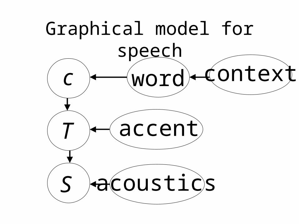
Graphical model for speech
c
S
T
acoustics
word context
accent
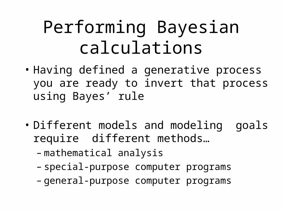
Performing Bayesian calculations
• Having defined a generative process you are ready to invert that process using Bayes’ rule
• Different models and modeling goals require different methods…– mathematical analysis– special-purpose computer programs– general-purpose computer programs

Mathematical analysis
• Work through Bayes’ rule by hand– the only option available for a long time!
• Suitable for simple models using a small number of hypotheses and/or conjugate priors
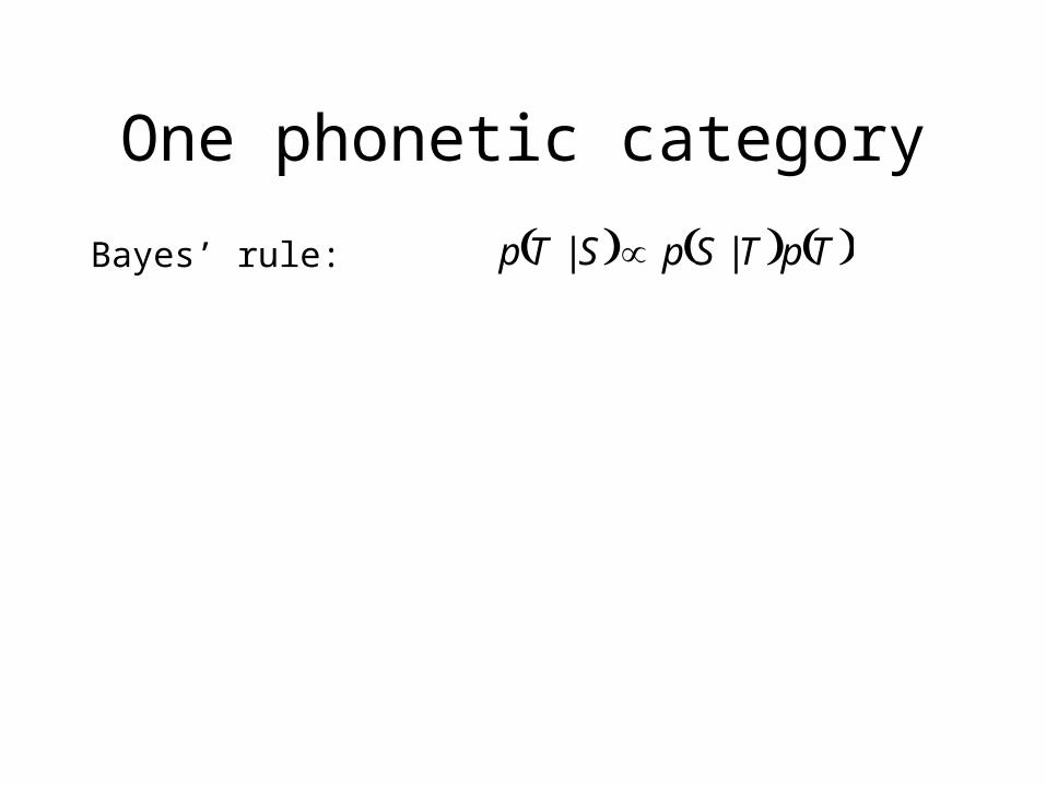
One phonetic category
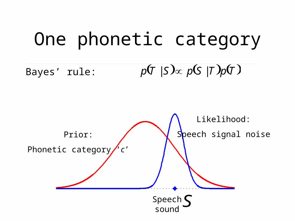
Bayes’ rule: ( ) ( ) ( )TpTSpSTp || ∝
One phonetic category
Bayes’ rule:
Prior:
Phonetic category ‘c’
Likelihood:
Speech signal noise
SSpeech sound
( ) ( ) ( )TpTSpSTp || ∝
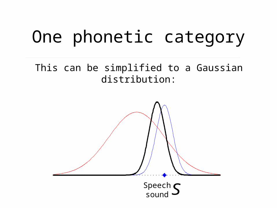
One phonetic category
This can be simplified to a Gaussian distribution:
Speech sound S
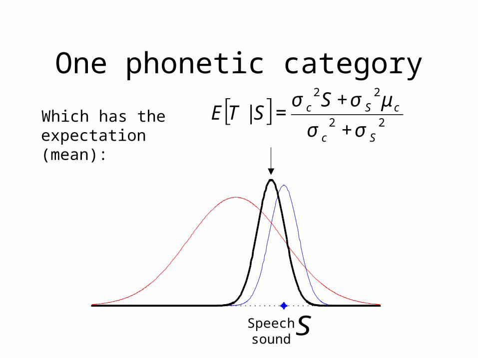
One phonetic category
Which has the expectation (mean):
[ ]22
22
|Sc
cSc SSTE
σσ
μσσ
+
+=
Speech sound
S
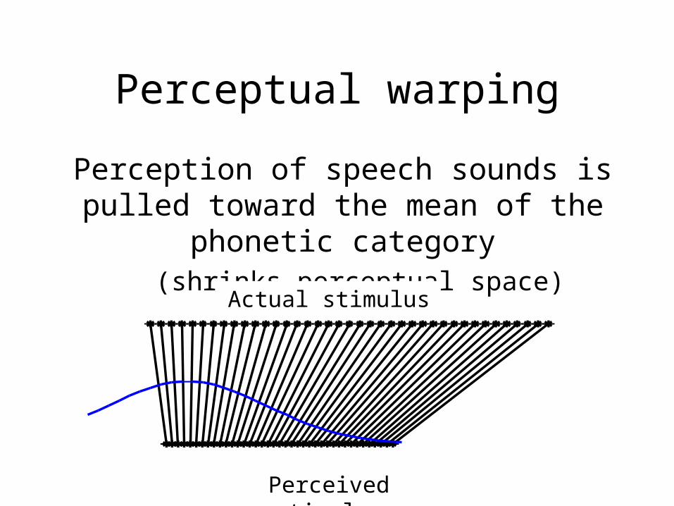
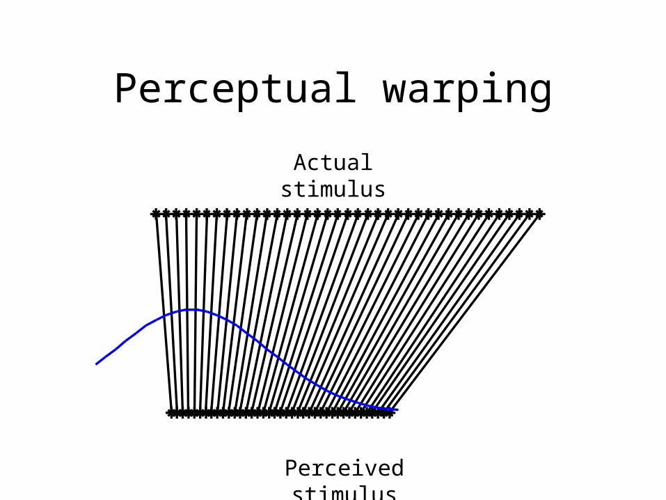
Perceptual warping
Perception of speech sounds is pulled toward the mean of the phonetic category
(shrinks perceptual space)
Actual stimulus
Perceived stimulus

Mathematical analysis
• Work through Bayes’ rule by hand– the only option available for a long time!
• Suitable for simple models using a small number of hypotheses and/or conjugate priors
• Can provide conditions on conclusions or determine the effects of assumptions– e.g. perceptual magnet effect
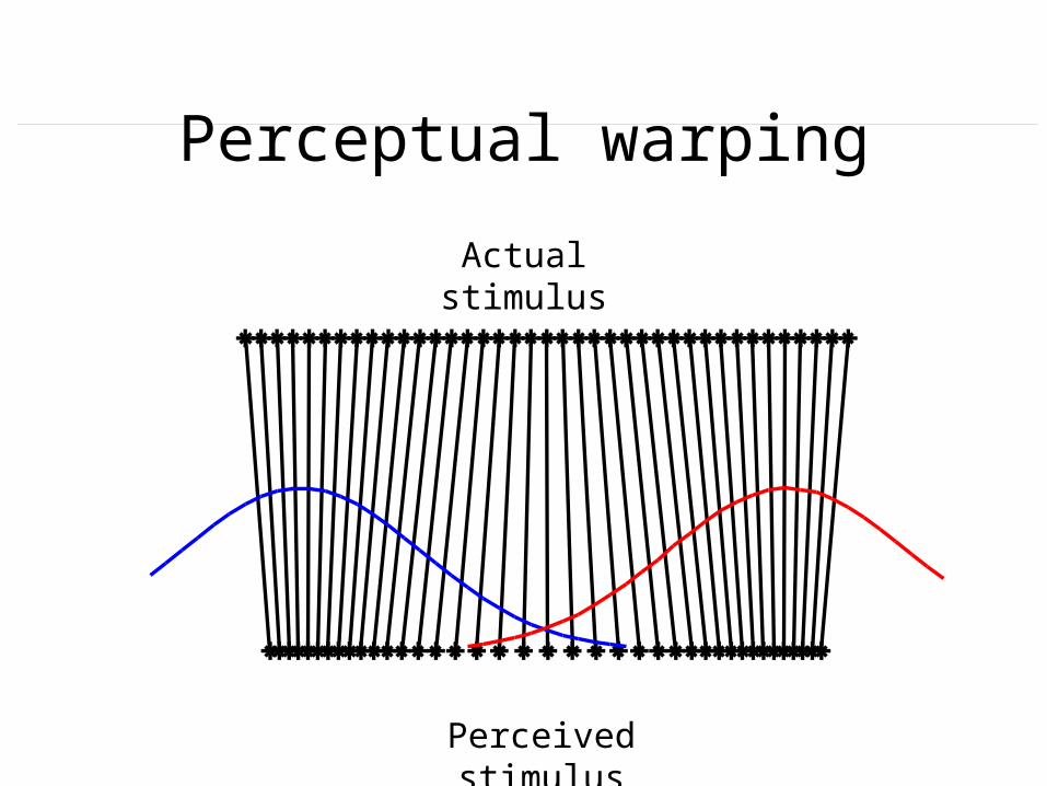
Perceptual warping
Actual stimulus
Perceived stimulus
Perceptual warping
Actual stimulus
Perceived stimulus
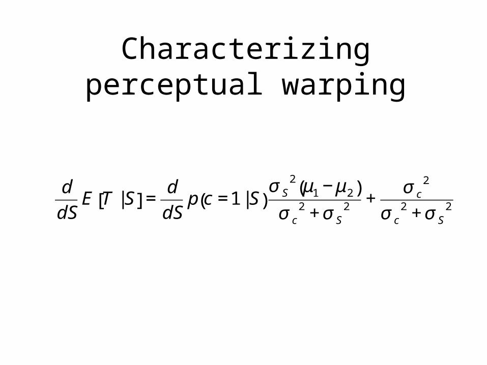
Characterizing perceptual warping
€
d
dSE T | S[ ] =
d
dSp c =1 | S( )
σ S2 μ1 − μ2( )
σ c2 + σ S
2 +σ c
2
σ c2 + σ S
2
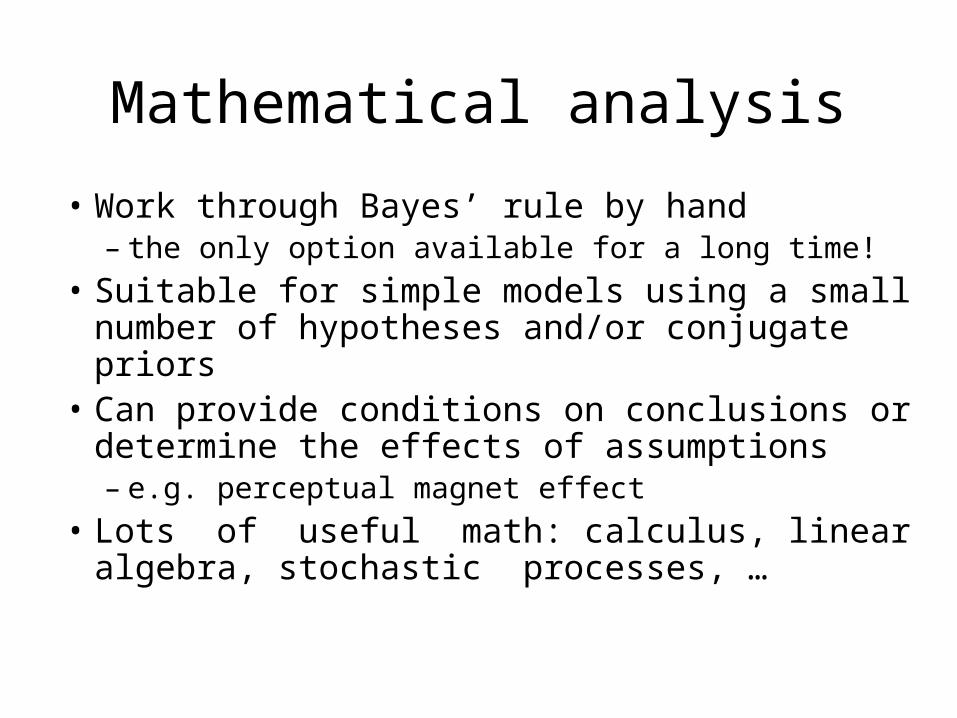
Mathematical analysis
• Work through Bayes’ rule by hand– the only option available for a long time!
• Suitable for simple models using a small number of hypotheses and/or conjugate priors
• Can provide conditions on conclusions or determine the effects of assumptions– e.g. perceptual magnet effect
• Lots of useful math: calculus, linear algebra, stochastic processes, …
Special-purpose computer programs
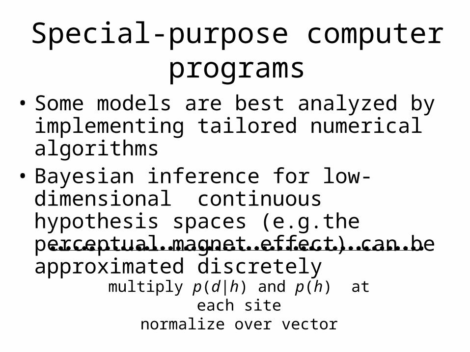
• Some models are best analyzed by implementing tailored numerical algorithms
• Bayesian inference for low-dimensional continuous hypothesis spaces (e.g.the perceptual magnet effect) can be approximated discretely
multiply p(d|h) and p(h) at each sitenormalize over vector
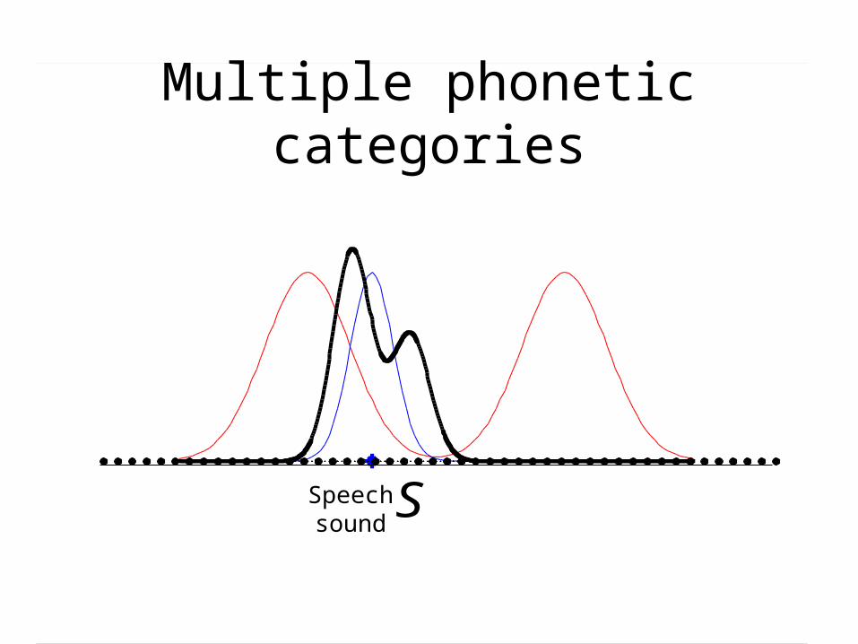
Multiple phonetic categories
SSpeech sound
Special-purpose computer programs
• Some models are best analyzed by implementing tailored numerical algorithms
• Bayesian inference for large discrete hypothesis spaces (e.g. concept learning) can be implemented efficiently using matrices
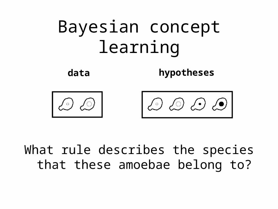
Bayesian concept learning
What rule describes the species that these amoebae belong to?
data hypotheses
Concept learning experiments
QuickTime™ and aTIFF (LZW) decompressor
are needed to see this picture.
data (d)
hypotheses (h)

Bayesian model(Tenenbaum, 1999; Tenenbaum & Griffiths, 2001)
€
P(h | d) =P(d | h)P(h)
P(d | ′ h )P( ′ h )′ h ∈H
∑d: 2 amoebaeh: set of 4 amoebae
€
P(d | h) =1/ h
m
0
⎧ ⎨ ⎩
d ∈ h
otherwise
m: # of amoebae in the set d (= 2)|h|: # of amoebae in the set h (= 4)
€
P(h | d) =P(h)
P( ′ h )h '|d ∈h'
∑ Posterior is renormalized prior
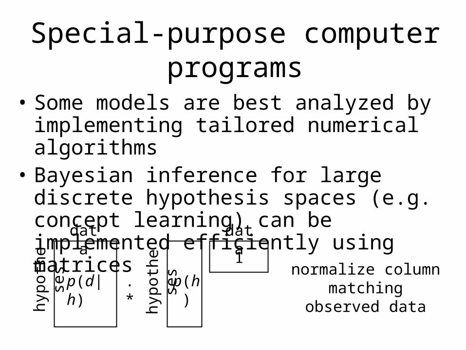
Special-purpose computer programs
• Some models are best analyzed by implementing tailored numerical algorithms
• Bayesian inference for large discrete hypothesis spaces (e.g. concept learning) can be implemented efficiently using matrices
data
hypo
thes
es
.*p(d|h)
hypo
thes
es
p(h)normalize column
matching observed data
data
1
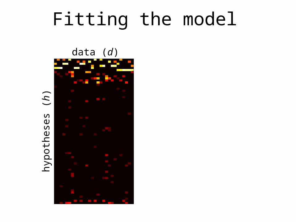
Fitting the model
data (d)hy
poth
eses
(h)
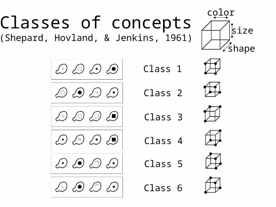
Classes of concepts(Shepard, Hovland, & Jenkins, 1961)
Class 1
Class 2
Class 3
Class 4
Class 5
Class 6
shape
size
color
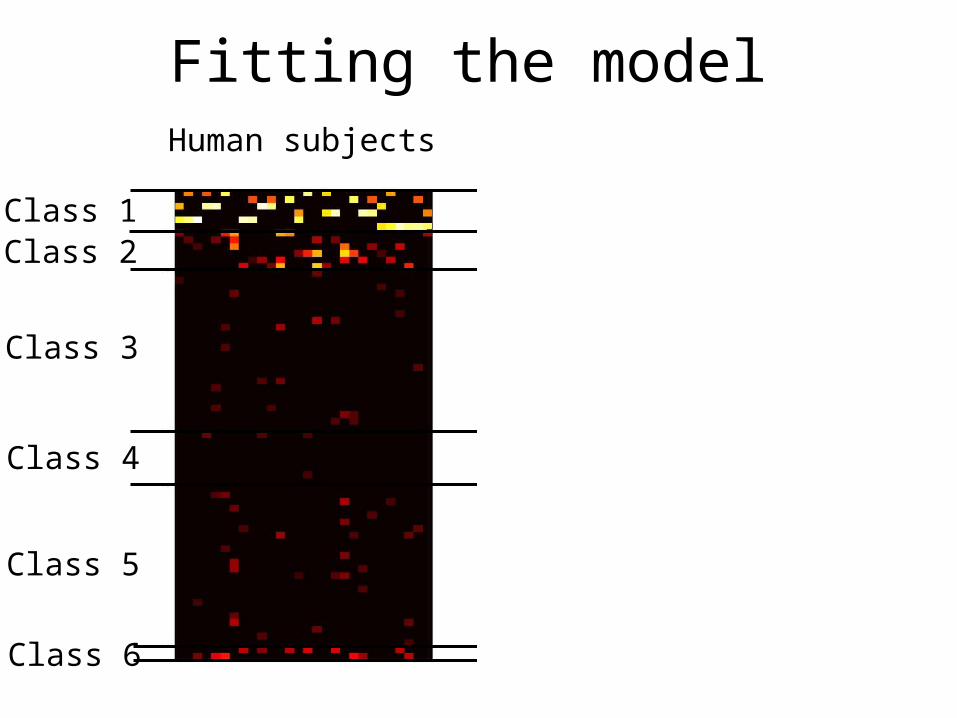
Fitting the model
Class 1Class 2
Class 3
Class 4
Class 5
Class 6
0.8610.087
0.009
0.002
0.013
0.028
Prior
r = 0.952
Bayesian modelHuman subjects

Special-purpose computer programs
• Some models are best analyzed by implementing tailored numerical algorithms
• Another option is Monte Carlo approximation…
• The expectation of f with respect to p can be approximated by
where the xi are sampled from p(x)
€
E p(x ) f (x)[ ] ≈1
nf (x i)
i=1
n
∑
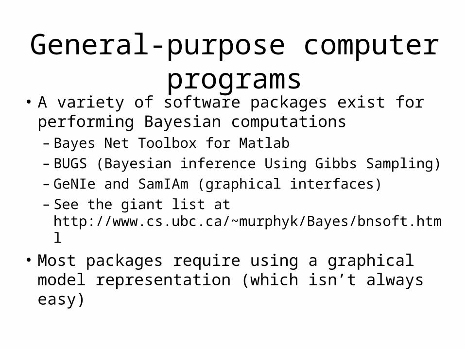
General-purpose computer programs
• A variety of software packages exist for performing Bayesian computations– Bayes Net Toolbox for Matlab– BUGS (Bayesian inference Using Gibbs Sampling)– GeNIe and SamIAm (graphical interfaces)– See the giant list at
http://www.cs.ubc.ca/~murphyk/Bayes/bnsoft.html
• Most packages require using a graphical model representation (which isn’t always easy)

Six easy steps
Step 1: Find an interesting aspect of cognition
Step 2: Identify the underlying computational problem
Step 3: Identify constraints
Step 4: Work out the optimal solution to that problem, given constraints
Step 5: See how well that solution corresponds to human behavior (do some experiments!)
Step 6: Iterate Steps 2-6 until it works
(Anderson, 1990)
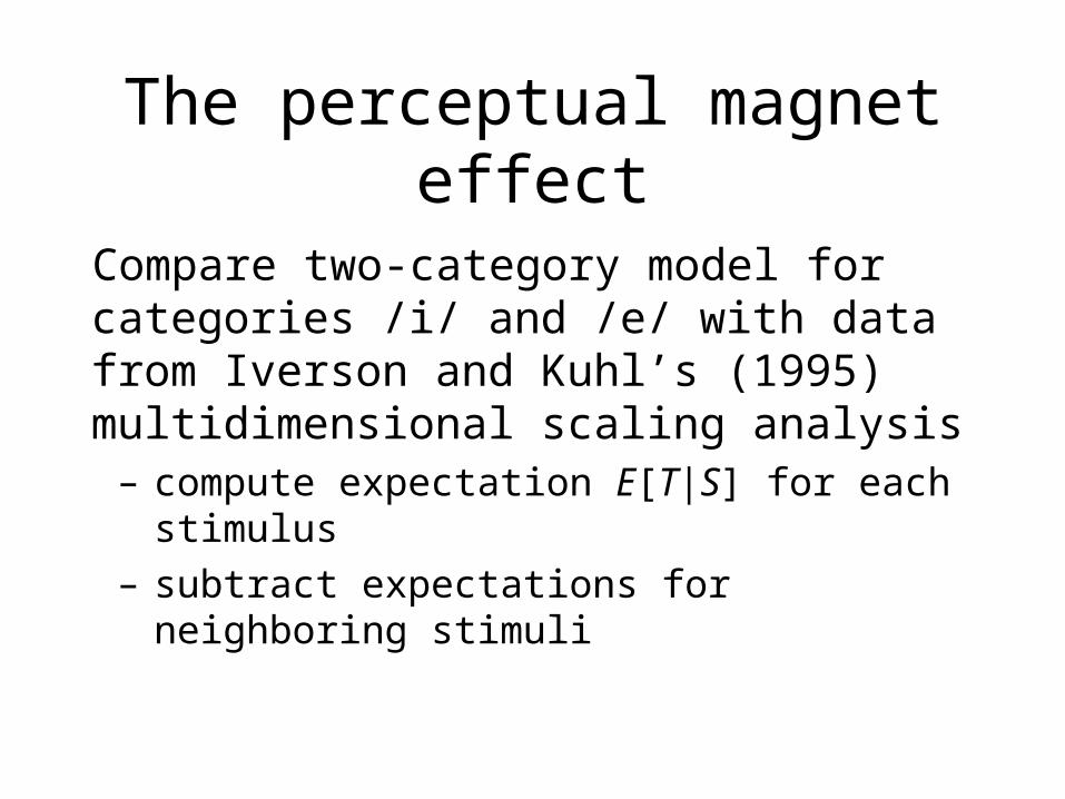
The perceptual magnet effect
Compare two-category model for categories /i/ and /e/ with data from Iverson and Kuhl’s (1995) multidimensional scaling analysis
– compute expectation E[T|S] for each stimulus– subtract expectations for neighboring stimuli
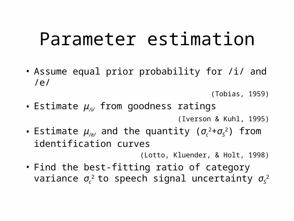
Parameter estimation
• Assume equal prior probability for /i/ and /e/(Tobias, 1959)
• Estimate μ/i/ from goodness ratings(Iverson & Kuhl, 1995)
• Estimate μ/e/ and the quantity (σc2+σS
2) from identification curves
(Lotto, Kluender, & Holt, 1998)
• Find the best-fitting ratio of category variance σc2 to
speech signal uncertainty σS2

Parameter values
μ/i/: F1: 224 Hz F2: 2413 Hz
μ/e/: F1: 423 Hz F2: 1936 Hz
σc: 77 mels
σS: 67 mels
Stimuli from Iverson and Kuhl (1995)
F2
(Mel
s)
F1 (Mels)
/i/
/e/
Quantitative analysisRelative Distances Between Neighboring
Stimuli
Stimulus Number
Rel
ativ
e D
ista
nce

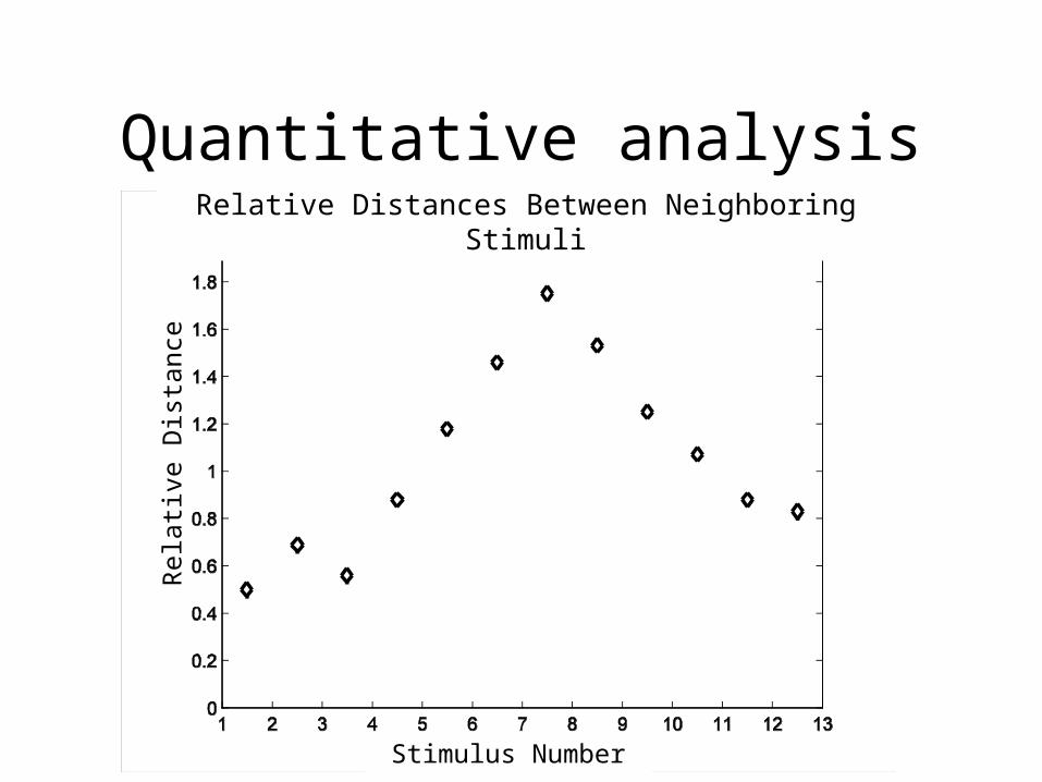
Quantitative analysisRelative Distances Between Neighboring
Stimuli
Stimulus Number
r = 0.97
Rel
ativ
e D
ista
nce
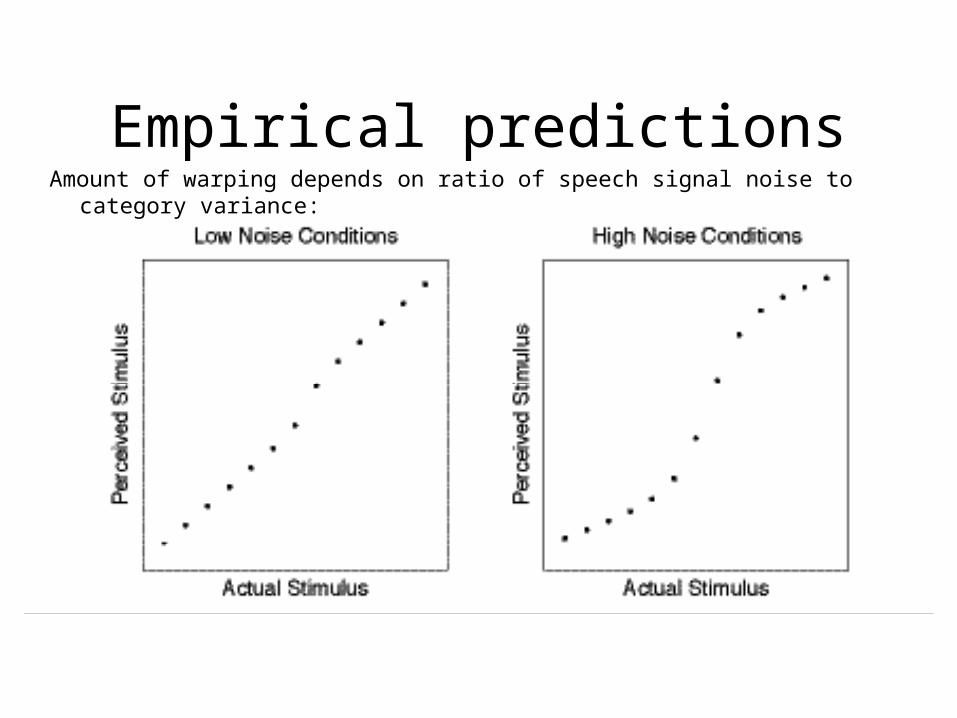
Empirical predictionsAmount of warping depends on ratio of speech signal noise to category variance:
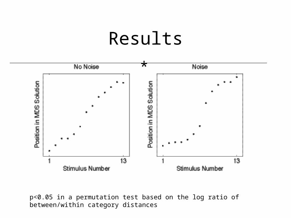
Results
*
p<0.05 in a permutation test based on the log ratio of between/within category distances
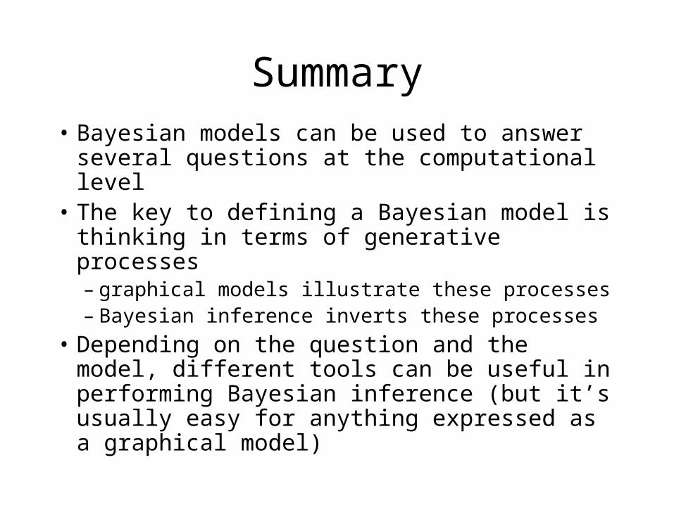
Summary
• Bayesian models can be used to answer several questions at the computational level
• The key to defining a Bayesian model is thinking in terms of generative processes– graphical models illustrate these processes– Bayesian inference inverts these processes
• Depending on the question and the model, different tools can be useful in performing Bayesian inference (but it’s usually easy for anything expressed as a graphical model)

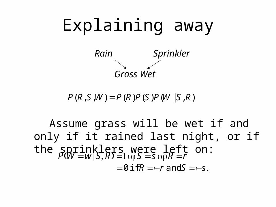
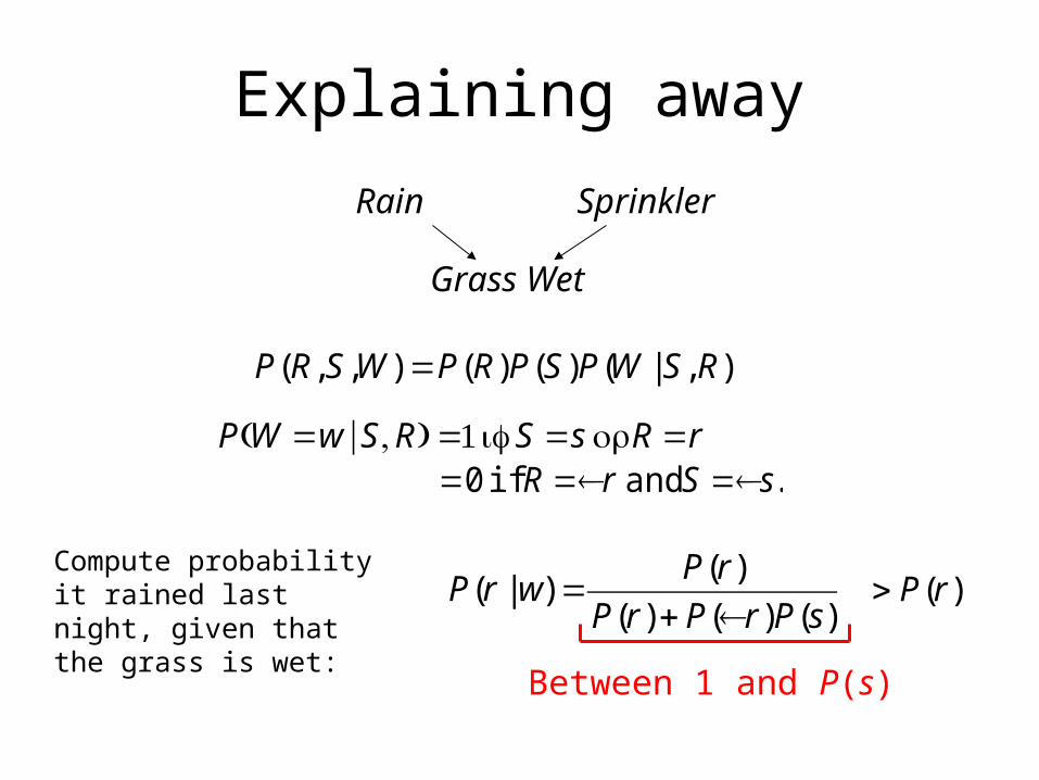
Assume grass will be wet if and only if it rained last night, or if the sprinklers were left on:
Explaining away
Rain Sprinkler
Grass Wet
.andif0 sSrR ¬=¬==
),|()()(),,( RSWPSPRPWSRP =
rRsSRSwWP ==== orif1),|(
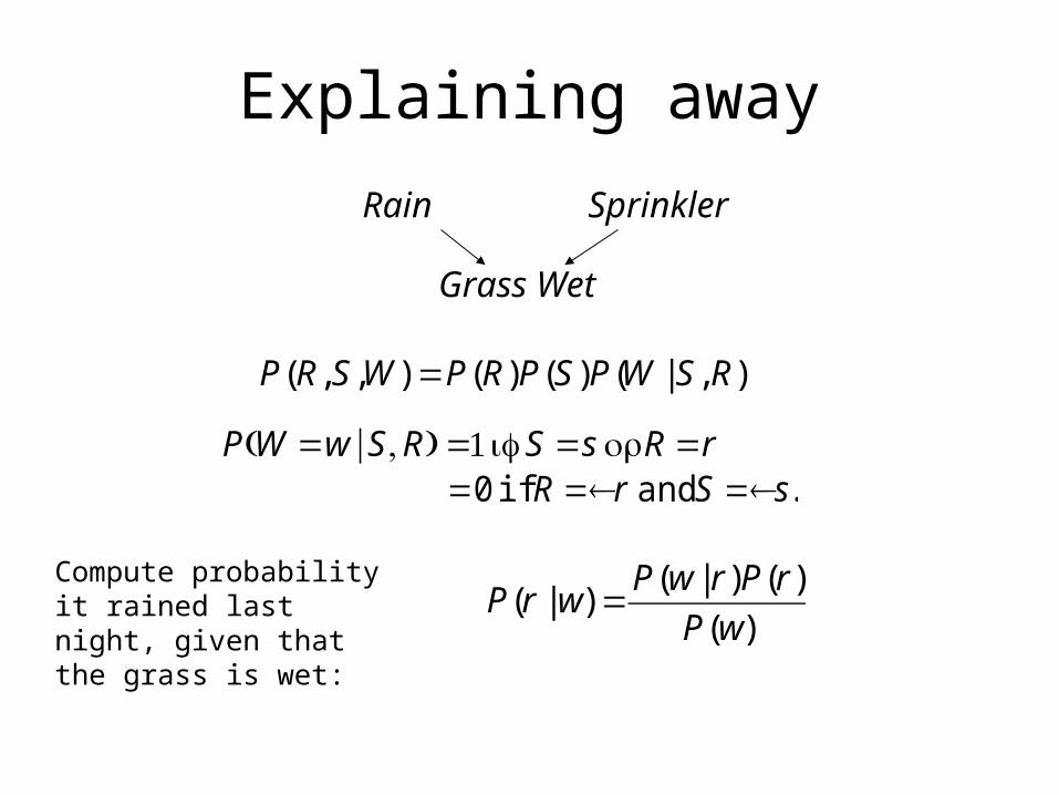
Explaining away
Rain Sprinkler
Grass Wet
)(
)()|()|(
wP
rPrwPwrP =
Compute probability it rained last night, given that the grass is wet:
.andif0 sSrR ¬=¬==
),|()()(),,( RSWPSPRPWSRP =
rRsSRSwWP ==== orif1),|(
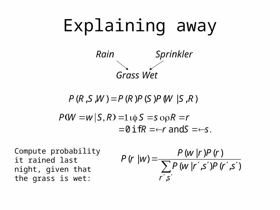
Explaining away
Rain Sprinkler
Grass Wet
∑′′
′′′′=
sr
srPsrwP
rPrwPwrP
,
),(),|(
)()|()|(
Compute probability it rained last night, given that the grass is wet:
.andif0 sSrR ¬=¬==
),|()()(),,( RSWPSPRPWSRP =
rRsSRSwWP ==== orif1),|(
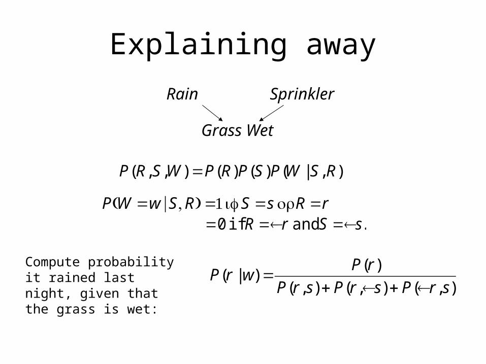
Explaining away
Rain Sprinkler
Grass Wet
),(),(),(
)()|(
srPsrPsrP
rPwrP
¬+¬+=
Compute probability it rained last night, given that the grass is wet:
.andif0 sSrR ¬=¬==
),|()()(),,( RSWPSPRPWSRP =
rRsSRSwWP ==== orif1),|(

Explaining away
Rain Sprinkler
Grass Wet
Compute probability it rained last night, given that the grass is wet:
),()(
)()|(
srPrP
rPwrP
¬+=
.andif0 sSrR ¬=¬==
),|()()(),,( RSWPSPRPWSRP =
rRsSRSwWP ==== orif1),|(
Explaining away
Rain Sprinkler
Grass Wet
)()()(
)()|(
sPrPrP
rPwrP
¬+=
Compute probability it rained last night, given that the grass is wet:
Between 1 and P(s)
)(rP>
.andif0 sSrR ¬=¬==
),|()()(),,( RSWPSPRPWSRP =
rRsSRSwWP ==== orif1),|(
Explaining away
Rain Sprinkler
Grass Wet
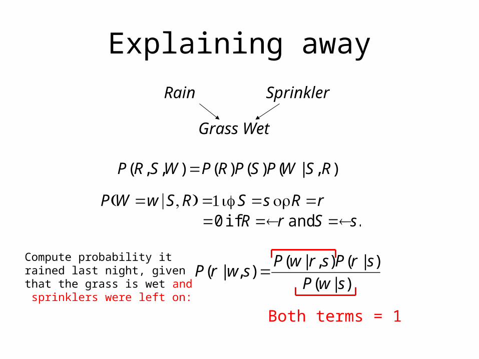
Compute probability it rained last night, given that the grass is wet and sprinklers were left on:
)|(
)|(),|(),|(
swP
srPsrwPswrP =
Both terms = 1
.andif0 sSrR ¬=¬==
),|()()(),,( RSWPSPRPWSRP =
rRsSRSwWP ==== orif1),|(
Explaining away
Rain Sprinkler
Grass Wet
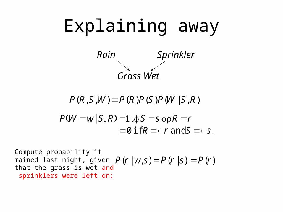
Compute probability it rained last night, given that the grass is wet and sprinklers were left on:
)(rP=)|(),|( srPswrP =
.andif0 sSrR ¬=¬==
),|()()(),,( RSWPSPRPWSRP =
rRsSRSwWP ==== orif1),|(

Explaining away
Rain Sprinkler
Grass Wet
)(rP=)|(),|( srPswrP =)()()(
)()|(
sPrPrP
rPwrP
¬+= )(rP>
“Discounting” to prior probability.
.andif0 sSrR ¬=¬==
),|()()(),,( RSWPSPRPWSRP =
rRsSRSwWP ==== orif1),|(

• Formulate IF-THEN rules:– IF Rain THEN Wet– IF Wet THEN Rain
• Rules do not distinguish directions of inference• Requires combinatorial explosion of rules
Contrast w/ production system
Rain
Grass Wet
Sprinkler
IF Wet AND NOT Sprinkler THEN Rain
• Observing rain, Wet becomes more active. • Observing grass wet, Rain and Sprinkler become more active• Observing grass wet and sprinkler, Rain cannot become less active. No explaining away!
• Excitatory links: Rain Wet, Sprinkler Wet
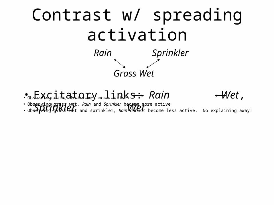
Contrast w/ spreading activation
Rain Sprinkler
Grass Wet
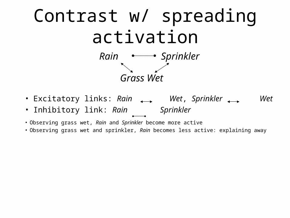
• Observing grass wet, Rain and Sprinkler become more active• Observing grass wet and sprinkler, Rain becomes less active: explaining away
• Excitatory links: Rain Wet, Sprinkler Wet
• Inhibitory link: Rain Sprinkler
Contrast w/ spreading activation
Rain Sprinkler
Grass Wet
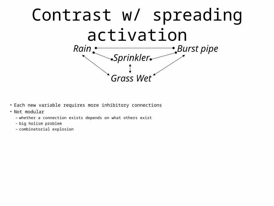
• Each new variable requires more inhibitory connections• Not modular
– whether a connection exists depends on what others exist– big holism problem – combinatorial explosion
Contrast w/ spreading activationRain
Sprinkler
Grass Wet
Burst pipe
Contrast w/ spreading activation
QuickTime™ and aTIFF (Uncompressed) decompressor
are needed to see this picture.
(McClelland & Rumelhart, 1981)
