part iv: sticky-price macroeconomics chapter … · the analysis of chapters 6 and 7 would explain...
TRANSCRIPT
Chapter 9 1 Final
PART IV: STICKY-PRICE MACROECONOMICSChapter 9: The Income-Expenditure Framework:
Consumption and the Multiplier
J. Bradford DeLong
Questions
What are "sticky" prices?
What factors might make prices sticky?
When prices are sticky, what determines the level of real GDP in the short run?
When prices are sticky, what happens to real GDP if some component of aggregate
demand falls?
When prices are sticky, what happens to real GDP if some component of aggregate
demand rises?
What determines the size of the spending multiplier?
Chapter 9 2 Final
Over the past decade real GDP in the American economy has grown at an average rate of
3.8 percent per year. At the same time, the American unemployment rate has fluctuated
around an average level consistent with stable inflation--a natural rate of
unemployment—of 4.5 percent. (Note, however, that this natural rate of unemployment
consistent with stable inflation is not a constant: it moves slowly over time.) And the
inflation rate in the United States has averaged about 2.5 percent per year.
If Chapters 4 through 8 gave a complete picture of the macroeconomy, economic growth
would be smooth. Real GDP would grow 3.8 percent—the current rate of growth of
potential GDP--year after year, not just on average. The unemployment rate would
remain steady at its natural rate of approximately 4.5 percent. And inflation would be
steady as well, determined by the rate of growth of potential output, of the money stock,
and the velocity of money.
If such were the case, the analysis of Chapters 4 and 5 would provide a complete picture
of how potential output grew over time. The analysis of Chapters 6 and 7 would explain
why real GDP equals potential output, and how national income is divided among the
different components of aggregate demand. The analysis of Chapter 8 would detail how
the price level and the inflation rate are determined. It would be the last chapter in this
textbook. Your survey of macroeconomics would be finished.
But Chapters 4 through 8 do not give a complete picture of the macroeconomy. Growth is
not at all smooth; on a year-to-year time scale, it is not even guaranteed. In 1982 real
GDP was not 3.8 percent more, but 2.1 percent less than it was in 1981. Between 1979
and 1982 the unemployment rate rose by 4.1 percentage points, and it rose again by 2.2

Chapter 9 3 Final
percentage points between 1989 and 1992. Unemployment may have been only 4.0% at
the end of 2000, but it was 7.6% in the middle of 1992. Inflation at the end of 2000 may
have been only 2.8% per year, but in 1981 it was 9.4%.
Figure 9.1: Real GDP per Worker and Potential Output, 1960-2000 [to be updated
every year]
Real GDP per Worker and Potential Output
$35
$40
$45
$50
$55
$60
1960 1970 1980 1990 2000
Years
Real GDP
PotentialOutput
Legend: The growth rate of potential output varies sharply from decade to decade.
From year to year real GDP fluctuates around potential output. The flexible-price
full-employment classical model of Chapters 6 and 7 does not account for these

Chapter 9 4 Final
large fluctuations in real GDP relative to potential output.
Source: Economic Report of the President.
These fluctuations in growth are called business cycles. A business cycle has two phases:
an exciting expansion or boom phase as production, employment, and prices all grow
rapidly; and a subsequent recession or depression phase during which inflation falls or
prices slump, unemployment rises, and production falls. During booms, output grows
faster than trend, investment spending amounts to a higher than average share of GDP,
unemployment falls, and inflation usually accelerates. During recessions, output falls,
investment spending is a low share of real GDP, unemployment rises, and inflation
usually decelerates.
9.1 Sticky Prices
Business Cycles
To understand business cycles, we need a model that does not guarantee always-full
employment, and in which real GDP does not always equal potential output. Business
cycles, after all, are not fluctuations in potential output but fluctuations of actual
production around potential output. Thus the full-employment model of Chapters 6
through 8 is of not help because its assumption that prices are flexible guarantees full
employment. The flexible-price assumption allowed us to start our analysis by noting the
labor market would clear with the supply of workers equal to the demand for labor, that

Chapter 9 5 Final
as a result firms would fully employ the labor force, and thus real GDP and household
income would be equal to potential output.
From this point forward, however, we need to break this flexible-price assumption in
order to build a more useful model of the business cycle. From this point forward prices
will be "sticky": they will not move freely and instantaneously in response to changes in
demand and supply. Instead, prices will remain fixed at predetermined levels as
businesses expand or contract production in response to changes in demand and costs. As
you will see, such "sticky prices" make a big difference in economic analysis; they will
drive a wedge between real GDP and potential output, and between the supply of workers
and the demand for labor. We will then be able to use this sticky-price model to account
for business-cycle fluctuations.
Building this sticky-price model of the macroeconomy will take up all of Section IV. In
this chapter, Chapter 9, we will focus on how, when prices are sticky, firms hire will or
fire workers and expand or cut back production based on whether their inventories are
falling or rising. Inventory adjustment is the key to understanding how the level of real
GDP can fall below and fluctuate around potential output. The second chapter of this
Section IV, Chapter 10, will focus on how changes in the Federal Reserve-controlled
interest rate affect the levels of investment, exports, and real GDP in the sticky-price
model.
The third chapter of this Section IV, Chapter 11, will begin to cover the monetary side of
the sticky-price model. First, it analyzes equilibrium in the money market; second, it
analyzes how the balance between aggregate demand and aggregate supply determine the

Chapter 9 6 Final
price level in the sticky-price model. The fourth and last chapter of this Section IV,
Chapter 12, will focus on expectations and inflation. And by the end of Chapter 12 we
will have linked up the sticky-price model of this Section IV with the flexible-price
model of the previous Section III. We will understand the sorts of situations for which the
sticky-price model is appropriate. And we will also understand under what sets of
circumstances wages and prices are flexible enough and have enough time to adjust for
the flexible-price model to be the most useful way of analyzing the macroeconomy.
At each stage in the building of our sticky-price macroeconomic model, the preceding
topic will serve as a necessary foundation. The analysis of inflation and expectations in
Chapter 12 will rest on the analysis of aggregate demand and aggregate supply in Chapter
11. The analysis of monetary equilibrium and aggregate demand in Chapter 11 will rest
on the analysis of how changes in interest rates affect investment, exports, and real GDP
in Chapter 10. And the analysis of Chapter 10 will in turn rest on the analysis of income,
expenditure, and equilibrium in a sticky-price economy carried out here in Chapter 9.
Up to this point this book has not been cumulative. You could understand the long-run
growth analysis of chapters 4 and 5 without a firm grasp of the introductory material in
chapters 1 through 3. You could understand the flexible-price analysis chapters 6 and 7
without a firm grasp of either the introductory or the long-run growth chapters. And you
could understand chapter 8 without having read anything earlier in the book. But from
this point on, this book becomes very cumulative indeed: Chapter 10 is incomprehensible
without a firm grasp of Chapter 9; Chapter 11 is incomprehensible without a firm grasp
of Chapter 10; Chapter 12 is incomprehensible without a firm grasp of Chapter 11; and
the chapters that follow 12 require it as well.
Chapter 9 7 Final
The Consequences of Sticky Prices
Flexible-Price Logic
To preview the difference between the flexible-price and the sticky-price models, let us
analyze a decline in consumers' propensity to spend under both sets of assumptions.
Suppose there is a sudden fall in the parameter C0 that determines the baseline level of
consumption in the consumption function:
C = C0 + Cy × Y
At any given level of national income Y, consumers wish to save more and spend less. To
make this concrete, suppose that the function for annual consumption spending (in
billions of dollars) declines from:
C = 2000 + 0.5 × Y
to:
C = 1800 + 0.5 × Y
In the full-employment model of chapters 6 through 8, a $200 billion fall in annual
consumption spending would have no impact on real GDP. No matter what the flow of
aggregate demand, because nominal wages and prices are flexible the labor market would
still reach its full-employment equilibrium as shown in Figure 9.2. And because the
economy remains at full employment real GDP would equal potential output.

Chapter 9 8 Final
Figure 9.2: Labor Market Equilibrium
Real wageW/P
Economy-wide demand for labor L
D
Labor supply = labor force
Equilibriumemployment
Market equilibriumreal wage
Legend: No matter what the flow of aggregate demand, flexible wages and prices
mean that employment remains at full employment, and the level of real GDP
produced remains at potential output.
The fall in consumption spending would have an effect on the economy--just not on the
level of real GDP. As we saw in Chapters 6 and 7, a fall in consumption spending means
an increase in savings. As consumption falls, the savings supply curve shifts rightward on
the flow-of-funds diagram, as Figure 9.3 shows. Thus a fall in consumption spending
reduces the equilibrium interest rate in the flow-of-funds market. It also increases the

Chapter 9 9 Final
equilibrium level of investment and net exports by $200 billion a year, the amount
necessary to keep GDP equal to potential output.
Figure 9.3: The Effect on Savings of a Fall in Consumption Spending in the Flexible-
Price Model
Real Interest Rater
Flow-of-Funds Through Financial Markets
Investment Demand
An increase in consumption spendingraises savings
...generatesa fall in the realinterest rate...
...and a rise in investment spending...
Savings Supply
Legend: A fall in consumption spending means a rise in private savings and an
increase in the supply flow of savings through financial markets. Thus the real
interest rate falls, and more investment projects are undertaken. The fall in the
real
interest rate also raises the value of the exchange rate, and boosts net exports.

Chapter 9 10 Final
Moreover, as we saw in Chapter 8, such a fall in the real rate has consequences for
money demand. Changes in households' and businesses' total demand for money M can
be triggered by a change in the price level P, real GDP Y, the banking system structure-
driven trend in the velocity of money VL, or the dependence of velocity on the nominal
interest rate. The higher the nominal interest rate i—which equals the real interest rate r
plus the expected future inflation rate π—the lower are households' and businesses'
demand to hold their wealth in the readily-spendable and liquid form of money.
M =P × Y
V L × (V0 + Vi × (r + π ))
If we rearrange this equation to solve for the equilibrium price level P:
P =M
Y
× V L × (V0 + Vi × (r +π ))( )
we see that a fall in the nominal interest rate means a fall in velocity and carries with it a
fall in the price level. A households and businesses try to divert some of their spending to
build up their stocks of liquid money, their actions put downward pressure on prices,
restoring equilibrium in the money market.
Thus these are the flexible-price model consequences of a fall in consumers' desired
baseline spending:
• Consumption falls.
• Savings rises.
• The real interest rate falls.
• Investment rises.
• The value of the exchange rate rises.

Chapter 9 11 Final
• The price level declines.
Sticky-Price Logic
If wages and prices are sticky, the analysis is different. The first consequence of
consumers cutting back their spending will be a fall in the aggregate demand for goods.
Consumer spending has fallen, yet nothing has happened to change the flow of spending
on investment goods, the flow of net exports, or the flow of government purchases.
As businesses see spending on their products begin to fall, they will not cut their nominal
prices (remember, prices are sticky). Instead, they will respond to the fall in the quantity
of their products demanded by reducing their production, They want to avoid
accumulating unsold and unsellable inventory. As they reduce production, they will fire
some of their workers, and the incomes of the fired workers will drop. By how much will
total national income drop? It will fall by the amount of the fall in consumption spending:
$200 billion a year. (Moreover, because the decline in incomes leads to a further decline
in consumption as households that have lost income cut back on their spending, national
incomes and real GDP would fall by more than the decline in C0. This multiplier process
is discussed later on in this chapter).
In sum, the consequences of a fall in consumption spending under the sticky-price
assumption are:
• Consumption falls.
• Production and employment decline.
• National income declines.

Chapter 9 12 Final
In the flexible-price model, when consumption falls investment and net exports rise. Why
doesn’t the same thing happen happen in the sticky-price model? Why doesn't a rise in
investment spending keep GDP equal to potential output and employment full? What
goes wrong with the flexible-price logic, according to which a fall in consumption
spending generates an increase in savings that then boosts both investment spending and
net exports?
The answer is that as firms cut back production and employment, total income falls. A
fall in total income reduces savings (if consumption is held constant) just as a fall in
consumption raises savings (if income is held constant). Under the sticky-price
assumption that effects on savings of the fall in consumption and the fall in income
cancel each other out: there is no change in the flow of savings. Thus there is no
rightward shift in the position of savings supply curve on the flow-of-funds diagram,
Figure 9.4. There is no fall in interest rates to trigger higher investment (and a higher
value of the exchange rate, and expanded net exports). There is nothing to offset the fall
in consumption spending and keep GDP from falling below potential output.
Figure 9.4: The Effect on Savings of a Fall in Consumption Spending in the Sticky-
Price Model
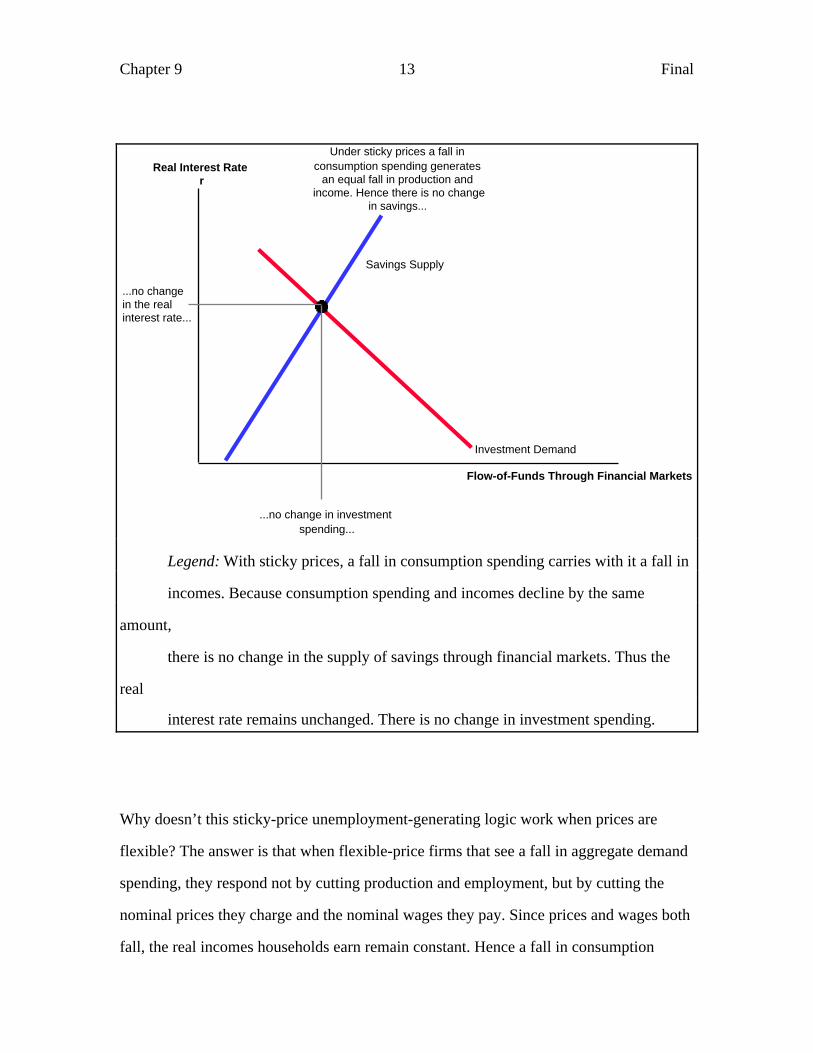
Chapter 9 13 Final
Real Interest Rater
Flow-of-Funds Through Financial Markets
Investment Demand
Under sticky prices a fall inconsumption spending generates
an equal fall in production and income. Hence there is no change
in savings...
...no changein the realinterest rate...
...no change in investment spending...
Savings Supply
Legend: With sticky prices, a fall in consumption spending carries with it a fall in
incomes. Because consumption spending and incomes decline by the same
amount,
there is no change in the supply of savings through financial markets. Thus the
real
interest rate remains unchanged. There is no change in investment spending.
Why doesn’t this sticky-price unemployment-generating logic work when prices are
flexible? The answer is that when flexible-price firms that see a fall in aggregate demand
spending, they respond not by cutting production and employment, but by cutting the
nominal prices they charge and the nominal wages they pay. Since prices and wages both
fall, the real incomes households earn remain constant. Hence a fall in consumption

Chapter 9 14 Final
spending does induce a rise in savings—hence a fall in the real interest rate, a rise in
investment spending, an increase in the value of the exchange rate, and a rise in net
exports
Expectations and Price Stickiness
Note that price stickiness causes problems only in the short run. If managers, workers,
consumers, and investors had time to foresee and gradually adjust their wages and prices
to a fall in consumption, even considerable stickiness in prices would not be a problem.
With sufficient advance notice unions and businesses would strike wage bargains, and
businesses could adjust their selling prices to make sure demand matches productive
capacity. Both the stickiness of prices and the failure to accurately foresee changes far
enough in advance are needed to create business cycles.
Thus one way to think about it is that the analysis of this Section IV is a "short run"
analysis, and the analysis of Section III is a "long run" analyses. In the short, run prices
are sticky; shifts in policy or in the economic environment that affect the components of
aggregate demand will affect real GDP and employment. In the long run, prices are
flexible and workers, bosses, and consumers have time to react and adjust to changes in
policy or the economic environment. Thus in the long run, such shifts do not affect real
GDP or employment.
Why do we need a short-run model as well as the long-run model of Section III? Why
isn’t it good enough to say that once wages and prices have fully adjusted (however long

Chapter 9 15 Final
that takes) unemployment will be back at its natural rate and real GDP equal to potential
output? The most famous and effective criticism of such let’s-look-only-at-the-long-run
analyses was made by John Maynard Keynes on page 88 of his 1924 Tract on Monetary
Reform. Criticizing one such long-run-only analysis, Keynes wrote that “‘in the long run’
[it] is probably true…. But this long run is a misleading guide to current affairs. In the
long run we are all dead. Economists set themselves too easy, too useless a task if in
tempestuous seasons they can only tell us that when the storm is long past the ocean will
be flat once more.”
Where is the line that divides the short run from the long run? Do we switch from living
in the short run of Section IV to the long run of Section III on June 19, 2005? No, we do
not. The long run is an analytical construct. A change can be considered "long run" if
enough people see it coming far enough in advance and have had time to adjust to it—to
renegotiate their contracts and change their standard operating procedures accordingly.
The length of the long run, and thus how many of us will be dead before it comes,
depends in turn on the degree of price stickiness and the process by which people form
their expectations—both key topics for research in modern macroeconomics.
Why Are Prices Sticky?
“Why are prices sticky?” you might ask. Why don't they adjust quickly and smoothly to
maintain full employment? Why do businesses respond to fluctuations in demand first by
hiring or firing workers and accelerating or shutting down their production lines? Why
don't they respond first by raising or lowering their prices.

Chapter 9 16 Final
Economists have identified any number of reasons that prices could be "sticky," but they
are uncertain which are most important. Some likely explanations are that:
• Managers and workers find that changing prices or renegotiating wages is costly,
hence best delayed as long as possible.
• Managers and workers lack information and so confuse changes in total economy-
wide spending with changes in demand for their specific products.
• The level of prices is as much a sociological as well as an economic variable--
determined as much by what values people think is "fair" as by the balance of supply
and demand. Workers take a cut in their wages as an indication that their employer
does not value them—hence managers avoid wage cuts because they fear the
consequences for worker morale.
• Managers and workers suffer from simple "money illusion"; they overlook the effect
of price-level changes when assessing the impact of changes in wages or prices on
their real incomes or sales.
Let’s look more closely at each of these likely explanations.
Economists call the costs associated with changing prices "menu costs," a shorthand
reference to the fact that when a restaurant changes its prices, it must print up a new
menu. In general, changing prices or wages may be costly for any of a large number of
reasons. Perhaps people wish to stabilize their commercial relationships by signing long-
term contracts. Perhaps reprinting a catalog is expensive. Perhaps customers find frequent
price changes annoying. Perhaps other firms are not changing their prices and what

Chapter 9 17 Final
matters most to a firm is its price relative to the price of competitors. Hence managers
and workers prefer to keep their prices and wages stable as long as the shocks that affect
the economy are relatively small—or rather as long as the change they might wish to
make in their prices and wages if changing them was costless is small.
A second source of price stickiness is misperception of real and nominal price changes. If
managers and workers lack full information about the state of the economy, they may be
unsure whether a change in the flow of spending on their products reflects a change in
overall aggregate demand or a change in demand for their particular products. If it is the
second, they should respond to by changing how much they produce and not necessarily
by changing the price. If it is the first, they should respond by changing their price in
accord with overall inflation and not by changing how much they produce.
If managers are uncertain which it is, they will split the difference. Hence firms will
lower their prices less in response to a downward shift in total nominal demand than the
flexible-price macroeconomic model would predict. If they keep their prices too high,
they will have to fire workers and cut back production.
Yet a third reason why prices and wages are sticky is that workers and managers are
really not the flinty-eyed rational maximizers of economc theories. In real life, work
effort and work intensity depends on whether workers believe they are being treated
fairly. A cut in your nominal wages is almost universally perceived as unfair; wages
depend on social norms that evolve slowly. Thus wages are by nature sticky. And if
wages are sticky, firms will find that its best response to shifts in demand is to hire and
fire workers rather than to change prices.

Chapter 9 18 Final
Last, workers, consumers, and managers confuse changes in nominal prices with changes
in real (that is, inflation-adjusted) prices. Firms react to higher nominal prices by
thinking falsely that it is more profitable to produce more, even though it isn't because
their costs have risen in proportion. Workers react to higher nominal wages by searching
more intensively for jobs and working more overtime hours, even though rises in prices
have erased any increase in the real purchasing power of the wage paid for an hour's
work. Such money illusion is a powerful generator of price stickiness and business cycle
fluctuations.
All these factors are potential sources of price stickiness. Your professor may have strong
views about which is most important, but I believe that our knowledge is more limited. I
am not sure the evidence is strong enough to provide clear and convincing support for
any particular single explanation as the most important one. A safer position is to remain
agnostic about the causes of sticky wages and prices, and so we will focus on analyzing
their effects.
9.2 Income and Expenditure
If prices are sticky, higher aggregate demand boosts production, which boosts incomes.
Higher incomes give a further boost to consumption, which in turn boosts aggregate
demand some more. Thus any shift in a component of aggregate demand upward or
downward leads to an amplified shift in total production because of the induced shift in

Chapter 9 19 Final
consumption, as Figure 9.5 shows. The early twentieth century British economist John
Maynard Keynes was one of the first to stress the importance of this multiplier process.
While in booms the multiplier process induces an upward spiral in production, in bad
times it is a source of misery. The downward shock is amplified as those who have been
thrown out of work cut back on their consumption spending in turn. Because
consumption spending is more than two thirds of aggregate demand, this multiplier effect
can be significant because the positive-feedback loop is so large.
Figure 9.5: The Multiplier Process
An initial shock to demandraises total spending...
Higher spendingraises production...
Higher productionraises incomes...
And higherincomes raisetotal spendingstill further.
Legend: In the multiplier process, an increase in spending causes an increase in
production and incomes, which leads to a further increase in spending. This
positive feedback loop amplifies the effect of any initial shift.

Chapter 9 20 Final
Building Up Aggregate Demand
In the remainder of this chapter we will see how the level of aggregate demand is
determined in the sticky-price macroeconomic model. We will use a bottom-up approach,
building aggregate demand or planned expenditure E on domestically-produced products
up from the determinants of each of its components, consumption spending C, investment
spending I, government purchases G, and net exports NX:
E = C + I + G + NX
As long as prices are sticky, the level of real GDP is determined by the level of aggregate
demand:
Y = E
and not by the level of potential output:
Y=Y*
The Consumption Function
The two-thirds of GDP that is consumption spending is spending by households on things
they find useful: services such as haircuts, nondurable goods such as food, and durable
goods such as washing machines. As incomes rise consumption spending rises with them,
increasing demand and setting the multiplier process in motion. As we saw in Chapter 6,
consumption spending does not rise dollar for dollar with total incomes. The share of an
extra dollar of disposable income that is added to consumption spending is the marginal
propensity to consume [ MPC] as shown in Figure 9.6, the parameter Cy in the
consumption function equation. The share of an extra dollar of national income that
shows up as additional consumption spending is equal to the marginal propensity to

Chapter 9 21 Final
consume times the share of income that escapes taxes: (1-t) Cy in the consumption
function equation:
C =C0+Cy (1 − t)Y
If changes in incomes are considered permanent, the MPC will be high: a $1 increase in
incomes will lead to an increase in consumption of as much as 80 cents. But if changes in
income are considered transitory, the MPC will be low: a $1 increase in incomes will lead
to an increase in consumption of only 30 cents or so. Transitory increases in income have
only a small effect on consumption because people seek to smooth out their consumption
spending over time.

Chapter 9 22 Final
Figure 9.6: The Consumption Function and the MPC
The Marginal Propensity to Consume
$0
$2,000
$4,000
$6,000
$8,000
$0 $2,000 $4,000 $6,000 $8,000 $10,000
Consumption Spending
National Income
Slope = MarginalPropensity to Consume
Legend: When drawn on a graph with economy-wide income on the
horizontal and consumption spending on the vertical axis, the slope of the
consumption function is the marginal propensity to consume.
For reasonably long-lasting shifts in the level of income, the MPC Cy is roughly 0.6. That
is, 60 cents of every extra dollar of disposable income shows up as higher consumption.
But remember that, as shown in Figure 9.7, when total consumption spending is plotted
against national income, the slope of the consumption function is smaller than the
parameter Cy because the tax system means that a one-dollar increase in national income
is a less than one-dollar increase in disposable income.
Chapter 9 23 Final
Box 9.1 shows how to use the consumption function and its parameters--the MPC, and
the tax rate—to calculate what consumption spending is.
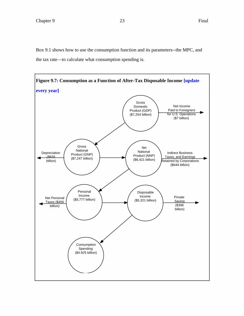
Figure 9.7: Consumption as a Function of After-Tax Disposable Income [update
every year]
GrossDomestic
Product (GDP)($7,254 billion)
Net IncomePaid to Foreignersfor U.S. Operations
($7 billion)
GrossNational
Product (GNP)($7,247 billion)
NetNational
Product (NNP)($6,421 billion)
Depreciation($826billion)
Indirect BusinessTaxes, and Earnings
Retained by Corporations($644 billion)
PersonalIncome
($5,777 billion)Net PersonalTaxes ($456
billion)
DisposableIncome
($5,321 billion)PrivateSaving($396billion)
ConsumptionSpending
($4.925 billion)

Chapter 9 24 Final
Legend: Three different factors drive the wedge between GDP and consumption
spending. The first is depreciation: goods produced that merely replace obsolete
and
worn-out capital and so are a component of total cost rather than total income.
The
second is the tax system--both direct and indirect taxes. And the third is private
savings.
Box 9.1--Example: Calculating the Consumption Function
Suppose statistical evidence tells us that the marginal propensity to consume out
of disposable income Cy is 0.75. Suppose further that taxes amount to 40 percent
of national income, and that when real GDP--total national income--equals $8
trillion then consumption equals to $5.5 trillion.
The fact that Cy is 0.6 and that the average tax rate t is 0.4 allows us to fill in some
of the parameters in the consumption function:
C = C0 + Cy × (1− t) × Y
C = C0 + 0.75 × (1 − 0.4) × Y
C = C0 + 0.45 × Y
We also know that when national income Y equals $8 trillion, consumption C
equals $5.5 trillion:

Chapter 9 25 Final
$5.5 = C0 + 0.45 × $8
$5.5 = C0 + $3.6
$1.9 = C0
So the numerical form of the consumption function is:
C = $1.9 + 0.45 × Y
The Other Components of Aggregate Demand [to be updated every year…]
The determinants of the other components of aggregate demand, investment spending,
government purchases, and net exports, are also familiar from Chapter six.

Chapter 9 26 Final
Figure 9.8: Components of Aggregate Demand [to be updated every year]
Components of Aggregate Demand in1995 (billions of 1992 dollars)
$4,578
$1,260
-$108
$1,010
$6,740
-$1,000
$0
$1,000
$2,000
$3,000
$4,000
$5,000
$6,000
$7,000
ConsumptionGovernmentPurchases Net Exports Investment
GrossDomesticProduct
Legend: By far the largest component of GDP is made up of consumption
spending. Government purchases come second, and gross investment comes third.
For the past two decades the United States has imported more than it has
exported;
hence net exports have been negative, not a contribution to but a subtraction from
GDP.
The level of investment spending, I, is determined by the real interest rate and
assessments of profitability made by business investment committees:

Chapter 9 27 Final
I = I0 − Ir × r
In our model we represent these determinants by making investment spending I a
function of the real interest rate r and of the parameters I0 and Ir, the baseline level of
investment spending and the interest sensitivity of investment.
The level of government purchases G is set by politics. Net exports are equal to gross
exports (a function of the real exchange rate ε and the level of foreign real GDP Yf)
minus imports. Imports are a function of national income Y:
NX = GX − IM = X fYf + Xεε( ) − IMyY
Figure 9.8 shows the relative sizes of these four components of aggregate demand.
Autonomous Spending and the Marginal Propensity to Expend
Let’s take the equation for aggregate demand:
E = C + I + G + NX
and replace the two components of aggregate demand that depend directly on national
income Y by their determinants:
E = C0 + Cy(1 − t)Y( ) + I + G + GX− IMyY( )
Chapter 9 28 Final
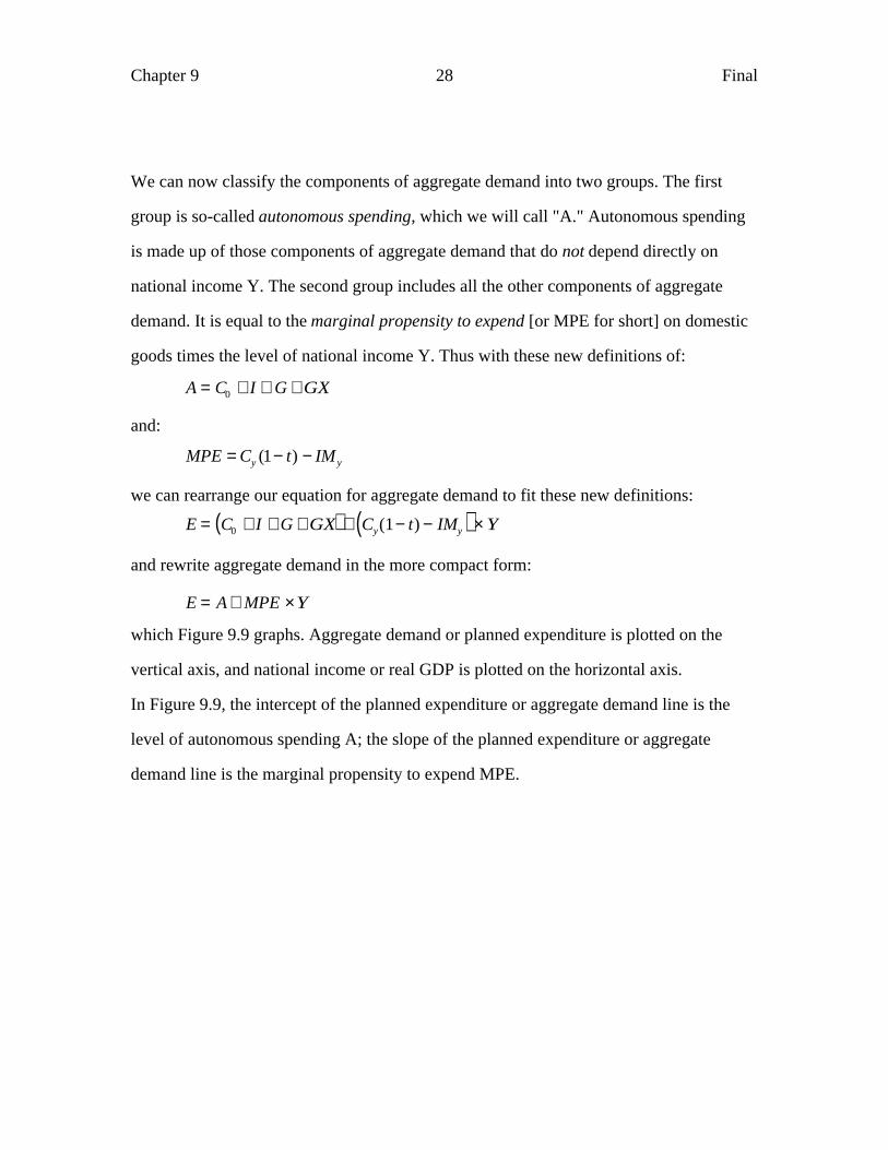
We can now classify the components of aggregate demand into two groups. The first
group is so-called autonomous spending, which we will call "A." Autonomous spending
is made up of those components of aggregate demand that do not depend directly on
national income Y. The second group includes all the other components of aggregate
demand. It is equal to the marginal propensity to expend [or MPE for short] on domestic
goods times the level of national income Y. Thus with these new definitions of:
A = C0 + I + G + GX
and:
MPE = Cy (1− t) − IM y
we can rearrange our equation for aggregate demand to fit these new definitions:
E = C0 + I + G + GX( ) + Cy(1− t) − IMy( ) × Y
and rewrite aggregate demand in the more compact form:
E = A + MPE ×Y
which Figure 9.9 graphs. Aggregate demand or planned expenditure is plotted on the
vertical axis, and national income or real GDP is plotted on the horizontal axis.
In Figure 9.9, the intercept of the planned expenditure or aggregate demand line is the
level of autonomous spending A; the slope of the planned expenditure or aggregate
demand line is the marginal propensity to expend MPE.

Chapter 9 29 Final
Figure 9.9: The Income-Expenditure Diagram
AggregateDemand,
or
PlannedExpenditure
Total Income, or Real GDP
AutonomousSpending
Slope = MPS
Planned Expenditure Line
Legend: On the income-expenditure diagram, the line showing the relationship
between total economy-wide income on the one hand total aggregate demand on
the other--the planned expenditure line--is determined by two things. Autonomous
spending is the level at which the planned expenditure line intercepts the y-axis.
The
marginal propensity to expend is the slope of the planned expenditure line.

Chapter 9 30 Final
Figure 9.10: An Increase in Autonomous Spending
AggregateDemand,
or
PlannedExpenditure
Total Income, or Real GDP
OldAutonomousSpending
Slope = MPS
Planned Expenditure Line
NewAutonomous
Spending
Legend: An increase in autonomous spending shifts the planned expenditure line
upward.
A change in the value of any determinant of any component of autonomous spending--the
baseline levels of consumption C0, of investment I0, or government purchases G; the real
interest rate r; and foreign-determined variables like foreign interest rates rf, foreign
levels of real income Yf, or speculators' view of exchange rate fundamentals ε0—will
shift the planned expenditure line up or down. The higher is autonomous spending, the
further from the x-axis the planned expenditure line will be (see Figure 9.10).
Changes in the marginal propensity to consume Cy, in the tax rate t, or in the propensity
to spend on imports IMy will change the MPE and the slope of the planned expenditure
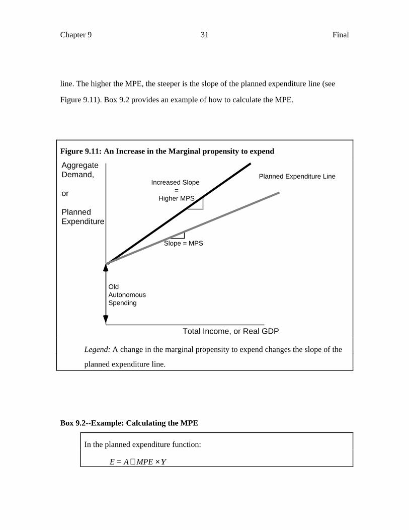
Chapter 9 31 Final
line. The higher the MPE, the steeper is the slope of the planned expenditure line (see
Figure 9.11). Box 9.2 provides an example of how to calculate the MPE.
Figure 9.11: An Increase in the Marginal propensity to expend
AggregateDemand,
or
PlannedExpenditure
Total Income, or Real GDP
OldAutonomousSpending
Slope = MPS
Planned Expenditure LineIncreased Slope
=Higher MPS
Legend: A change in the marginal propensity to expend changes the slope of the
planned expenditure line.
Box 9.2--Example: Calculating the MPE
In the planned expenditure function:
E = A + MPE ×Y

Chapter 9 32 Final
the marginal propensity to expend [MPE] will be less than the slope of the
consumption function Cy(1-t) because of the effect on the economy of imports.
The MPE is:
MPE = Cy(1− t) − IM y( )Thus if the marginal propensity to consume Cy is 0.75 and the tax rate is 40%, the
0.45 slope of the consumption function is an upper bound to the MPE. If imports
are 15 percent of real GDP, then:
MPE = Cy(1− t) − IM y( )MPE = 0.75 × (1 − 0.4) − .15( )MPE = .45 − .15 = .30
Such relatively small values of the MPE are typical for modern industrialized
economies, which have substantial amounts of international trade (that is,
relatively high values for IMy), large social-democratic social-insurance states
(that is, relatively high values for t), and deep and well-developed financial
systems that provide ample room for household borrowing and lending to smooth
out consumption (that is, relatively small values for Cy as well).
However, in the past, in relatively closed economies, or in economies with
undeveloped financial systems, the MPE can be significantly higher.
Sticky-Price Equilibrium

Chapter 9 33 Final
The economy will be in equilibrium when planned expenditure equals real GDP--which
is, according to the circular flow principle, the same as national income. Under these
conditions there will be no short-run forces pushing for an immediate expansion or
contraction of national income, real GDP, and aggregate demand.
Figure 9.12: Equilibrium on the Income-Expenditure Diagram
The Income-Expenditure Diagram (for1996; in Billions of Dollars)
$2,000
$4,000
$6,000
$8,000
$10,000
$2,000 $4,000 $6,000 $8,000 $10,000
Aggregate demandas a function ofNational Income
Equilibrium Point
National Income (alternatively, National Product or GDP)
Planned Expenditure(alternatively, Aggregate Demand)
Legend: On the income-expenditure diagram, the equilibrium point of the
economy
is that point where aggregate demand (as a function of total product) is equal to
total
product.

Chapter 9 34 Final
On the income-expenditure diagram, those points at which planned expenditure equals
national income are a line running up and to the right at a 45-degree angle with respect to
the x-axis, as see Figure 9.12 shows. This line covers all the possible points of
equilibrium. The actual equilibrium will be that point at which planned expenditure is
equal to national income. The point where this planned expenditure line intersects the 45-
degree equilibrium condition line is the economy's equilibrium.
In algebra, the equilibrium values of aggregate demand E and real GDP or national
income Y must satisfy both:
E = A + MPE ×Y
and:
E = Y
Substituting Y in for E in the first of these equations and regrouping, the solution is:
Y = E =A
1 − MPE
If the numerical values of the parameters of the planned expenditure function:
E = A + MPE ×Y
are (in billions) A = $5600 and MPE = 0.3, then planned expenditure as a function of real
GDP is:
E = 5600 + 0.3 × Y
The equilibrium level of real GDP and aggregate demand is then (in billions):
Y = $8000

Chapter 9 35 Final
Figure 9.13: Inventory Adjustment and Equilibrium
Planned Expenditure(alternatively, Aggregate Demand)
National Income (alternatively, National Product or GDP)
$-
$2,000
$4,000
$6,000
$8,000
$- $2,000 $4,000 $6,000 $8,000 $10,000
Income = Expenditure
Fallinginventories
Risinginventories
Goods market equilibrium
Aggregate Demand(or Planned Expenditure)
Goods Market Equilibrium and theIncome-Expenditure Diagram
Legend: If the economy is not at its equilibrium point, then either total production
exceeds aggregate demand (in which case inventories are rising) or aggregate
demand exceeds total production (in which case inventories are falling).
If the economy is not on the 45-degree line, then aggregate demand E does not equal real
GDP Y. If Y is greater than E, there is excess supply of goods. If E is greater than Y,
there is excess demand for goods. In neither case is the economy in equilibrium.

Chapter 9 36 Final
In the first case in which production exceeds demand, inventories are rising rapidly and
firms unwilling to accumulate unsold and unsellable inventories are about to cut
production and fire workers (see Figure 9.13). In the second case in which demand
exceeds production, inventories are falling rapidly. Businesses are selling more than they
are making. Some businesses will respond to the fall in inventories by boosting prices,
trying to earn more profit per good sold. But the bulk of businesses will respond to the
fall in inventories by expanding production to match demand. They are about to hire
more workers. Real GDP and national income are about to expand.
Now suppose that businesses see their inventories falling, and respond by boosting their
production to equal last month's planned expenditure. Will such an increase bring the
economy into goods-market equilibrium, with planned expenditure equal to total income
and real GDP? The answer is that it will not. To boost production, firms must hire
workers, paying more in wages, and causing household incomes to rise. When income
rises, total spending rises as well. Thus the increase in production and income generates a
further expansion in aggregate demand.

Chapter 9 37 Final
Figure 9.14: The Inventory Adjustment Process
National Income (alternatively, National Product or GDP)
Income-Expenditure Diagram
$-
$2,000
$4,000
$6,000
$8,000
$- $2,000 $4,000 $6,000 $8,000 $10,000
InitialExpenditure
NewExpenditure
Planned Expenditure(alternatively, Aggregate Demand)
Legend: If planned expenditure is greater than total production and inventories are
falling, businesses will hire more workers and increase production.
Even after production has increased to close the initial gap between aggregate demand
and national income, as Figure 9.14 shows the economy will still not be in equilibrium.
Inventories will still be falling even though hiring more workers has increased
production. Because hiring more workers has also boosted total income and further
increased aggregate demand, production will have to expand by a multiple of the initial
gap in order to stabilize inventories. The process will come to an end, with aggregate

Chapter 9 38 Final
demand equal to national income, only when both have risen to the level at which the
planned expenditure line crosses the 45-degree income-equals-expenditure line. And the
process works in reverse if planned expenditure is below national income.
Box 9.3--Details: How Fast Does the Economy Move to Equilibrium?
At any one particular moment the economy does not have to be in short-run
equilibrium. Aggregate demand can exceed real GDP and national income and
inventories can fall for periods as long as a year. There are strong forces pushing
the economy toward short-run equilibrium. Businesses do not like to lose money
by producing things that they cannot sell, or by not having things on hand that
they could sell. But it takes at least months, usually quarters, and possibly more
time for businesses to expand or cut back production
For example, between the summer of 1990 and the summer of 1991 inventories
fell for five straight quarters. Real GDP was less than aggregate demand as
businesses decided that their high levels of inventories were too large given the
economic uncertainties created by the Iraqi invasion of Kuwait and the
subsequent recession.
Between the winter of 1994 and the summer of 1995, for six quarters, inventories
rose. For a year and a half GDP was greater than aggregate demand.

Chapter 9 39 Final
Figure 9.15: Inventories as the Balancing Item
Inventory Investment in the 1990s (Billions of Dollars per Year)
-$40
-$20
$0
$20
$40
$60
$80
1990 1991 1992 1993 1994 1995 1996
Average
Inventory investmentstrongly positive: nationalproduct ahead of aggregate
demand
Inventory investmentstrongly negative: aggregatedemand larger than national
product
Box 9.4--Details: Inventory Adjustment and the Circular Flow
The economy can be out of equilibrium, with planned expenditure either higher or
lower than national income and GDP. Yet by the definition of the circular flow,
economy-wide total expenditure always equals national income or GDP. We
would think that total expenditure is the same thing as aggregate demand. So isn’t
there a contradiction here?

Chapter 9 40 Final
The answer is that statisticians who compile the national income and product
accounts (NIPA) define "total expenditure" in a peculiar way. When production is
greater than spending and inventories pile up unexpectedly, the national income
accountants say the producing company has made an "investment expenditure": it
has spent money increasing its inventory.
Suppose Mammoth Motors produces an extra 100,000 cars, valued at $15,000
each, which it then fails to sell. Mammoth thus has the unpleasant surprise of
seeing its inventory rise by 100,000 cars: an unexpected inventory increase of
$1.5 billion. For Mammoth this is a disaster--it spent a huge sum making things it
could not sell that are now sitting in parking lots across the nation. But NIPA
statisticians record this as an "expenditure" by Mammoth: an investment in
inventories of $1.5 billion. Never mind that Mammoth certainly did not want to
make this "investment."
The NIPA system is set up to call all changes in every business's inventory a
positive or negative "investment expenditure" by that business in order to make
the circular flow principle hold by definition. Thus from the NIPA point of view
(save for accounting definitions and the statistical discrepancy), national income
and GDP have to be equal to total expenditure.
We do not want to pick a fight with the national income accountants, but we do
want to be able to speak of production greater than demand or demand greater
than production. So we finesse the issue by making a subtle distinction between
the investment spending that goes into our macroeconomic model and the
Chapter 9 41 Final
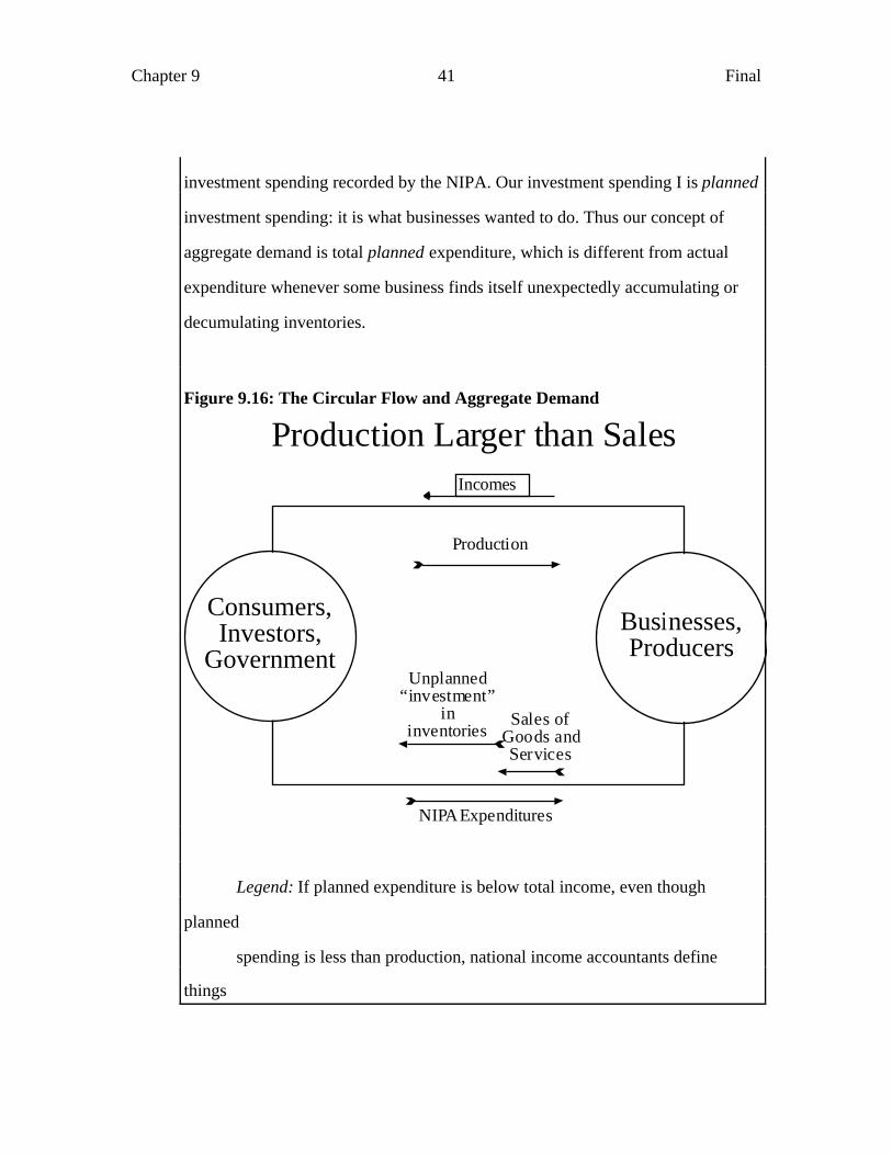
investment spending recorded by the NIPA. Our investment spending I is planned
investment spending: it is what businesses wanted to do. Thus our concept of
aggregate demand is total planned expenditure, which is different from actual
expenditure whenever some business finds itself unexpectedly accumulating or
decumulating inventories.
Figure 9.16: The Circular Flow and Aggregate Demand
Consumers,Investors,
Government
Businesses,Producers
Production
Sales ofGoods andServices
NIPAExpenditures
Production Larger than Sales
Unplanned“investment”
ininventories
Incomes
Legend: If planned expenditure is below total income, even though
planned
spending is less than production, national income accountants define
things

Chapter 9 42 Final
to make the circular flow principle--according to which spending is equal
to
production--hold. Unplanned business inventory accumulation is counted
as
spending. Thus it is important to remember that aggregate demand is equal
to planned expenditure, not to total spending as the NIPA reports it.
Box 9.5—An Example: Calculating the Difference Between Aggregate Demand and
Real GDP
Suppose that our planned expenditure function has numerical values for its
coefficients, so that in trillions:
E = A + MPE ×Y
E = $5.6 + 0.3 × Y
Suppose, first, that the current level of real GDP Y is $7.5 trillion. Then aggregate
demand--total planned expenditure--is:
E = $5.6 + 0.3 × $7.5
E = $7.85
And business inventories are being drawn down at a rate:
∆(Inventories)
∆(time)= Y − E = −$350 billion / year
Suppose, second, that the current level of total real GDP Y is $9.5 trillion. Then
total planned expenditure is:

Chapter 9 43 Final
E = $5.6 + 0.3 × $8.5
E = $8.35
And business inventories are being added to at a rate:
∆(Inventories)
∆(time)= $350 billion / year
However, if the current level of total national income (and of real GDP) Y is $9.0
trillion, then total planned expenditure is:
E = $5.6 + 0.3 × $8.0
E = $8.0
And business inventories are stable:
∆(Inventories)
∆(time)= $0
9.3 The Multiplier
Determining the Size of the Multiplier
Suppose something happens to change the level of planned expenditure at every possible
level of total income. Anything that affects the level of autonomous spending will do.
What would happen to the equilibrium level of total income and real GDP?
Chapter 9 44 Final
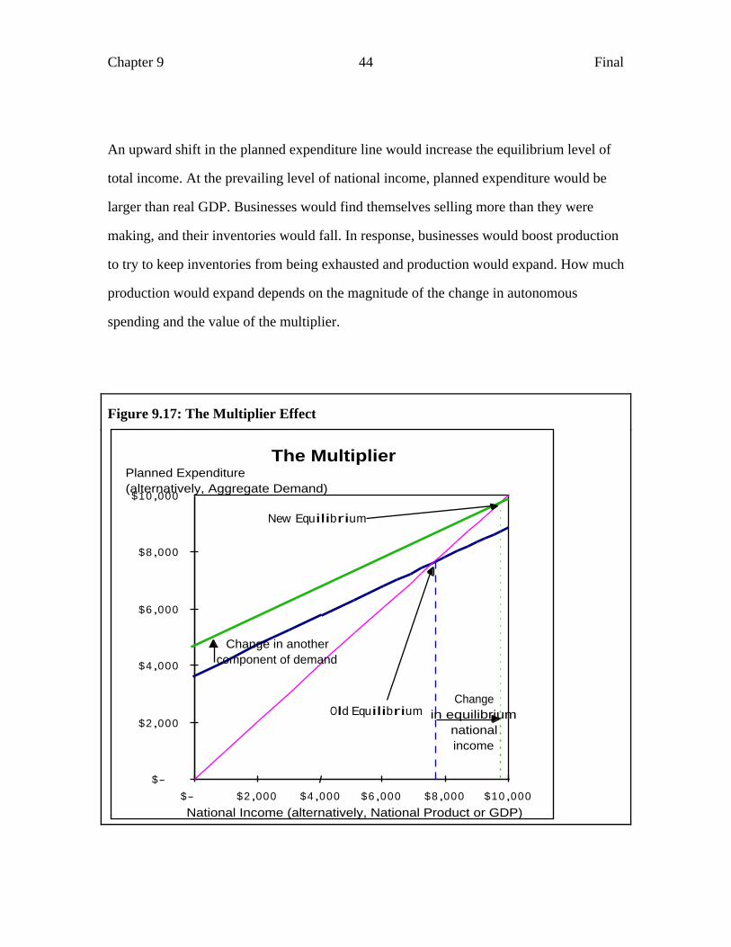
An upward shift in the planned expenditure line would increase the equilibrium level of
total income. At the prevailing level of national income, planned expenditure would be
larger than real GDP. Businesses would find themselves selling more than they were
making, and their inventories would fall. In response, businesses would boost production
to try to keep inventories from being exhausted and production would expand. How much
production would expand depends on the magnitude of the change in autonomous
spending and the value of the multiplier.
Figure 9.17: The Multiplier Effect
$-
$2,000
$4,000
$6,000
$8,000
$10,000
$- $2,000 $4,000 $6,000 $8,000 $10,000
Old Equilibrium
New Equilibrium
Planned Expenditure(alternatively, Aggregate Demand)
National Income (alternatively, National Product or GDP)
The Multiplier
Change in anothercomponent of demand
Changein equilibrium
nationalincome
Chapter 9 45 Final
Legend: An increase in autonomous spending will generate an amplified increase
in
the equilibrium level of national income. Why? Because planned expenditure will
rise not just by the increase in autonomous spending, but by the increase in
autonomous spending plus the marginal propensity to expend times the increase
in
the equilibrium level of national income.
The value of the multiplier depends on the slope of the planned expenditure line, the
marginal propensity to expend [MPE]. The higher is the MPE, the steeper is the planned
expenditure line and the greater is the multiplier. A large multiplier can amplify small
shocks to spending patterns into large changes in total production and income, as Figure
9.17 shows.
Chapter 9 46 Final
Figure 9.18: Determining the Size of the Multiplier
Change in nationalincome equals
change in autonomousspending
A
The Multiplier
$-
$2,000
$4,000
$6,000
$8,000
$- $2,000 $4,000 $6,000 $8,000 $10,000
1-c
New Equilibrium
National Income (alternatively, National Product or GDP)
Planned Expenditure(alternatively, Aggregate Demand)
Old Equilibrium
New Aggregate Demand
Old Aggregate Demand
Change in autonomous spending A
Legend: An increase ∆A in national income and total production raises the level
of
aggregate demand consistent with equilibrium by ∆A, but it also
raises the level of planned expenditure by the MPE x ∆A. A ∆A dollar
increase in national income and total production reduces the gap between total
production and planned expenditure by only (1 - MPE) ∆A. Hence the increase in
the equilibrium level of national income produced by a change ∆A in autonomous
spending is not ∆A, but ∆A/(1-MPE)-- ∆A times the value of the multiplier.
To calculate the multiplier, recall the simplified equation for planned expenditure:
E = A + MPE ×Y

Chapter 9 47 Final
And the equilibrium condition:
Y = E
Substitute the second into the first, and solve for Y:
Y =A
1 − MPE
Thus if autonomous spending changes by an amount ∆A, equilibrium real GDP changes
by:
∆Y =1
1 − MPE× ∆A
And if we want to express the denominator of this fraction in terms of the basic
parameters of the model, it is:
∆Y =1
1 − Cy (1 − t) − IMy( ) × ∆A
This factor 1/(1-MPE) = 1/(1-(Cy(1-t)-IMy)) is the multiplier: it multiplies the upward
shift in the planned expenditure line as a result of the increase in autonomous spending
into a change in the equilibrium level of real GDP, total income, and aggregate demand.
Why the factor 1/(1-MPE)? Think of it this way. The MPE--the marginal propensity to
expend--is the slope of the planned expenditure line. A $1 increase in national income
raises the equilibrium level of planned expenditure by $1, because expenditure has to go
$1 higher to balance income and production. As Figure 9.18 shows, it also raises the level
of planned expenditure by $MPE. Thus a $1 increase in the level of total income closes
$(1-MPE) of the gap between planned expenditure and total income. To close a full
initial gap of $∆A between planned expenditure and national income, the equilibrium
level of national income must increase by ∆A/(1-MPE).
Chapter 9 48 Final
Because autonomous spending is influenced by a great many factors:
A = C0 + I0 − Ir × r( ) + G + (X f × Y f + εr × ε0 − εr × r +εr × r f )
almost every change in economic policy or the economic environment will set the
multiplier process in motion.
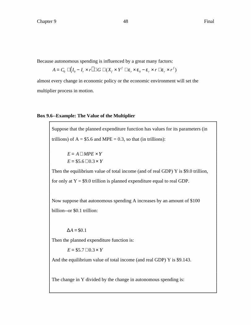
Box 9.6--Example: The Value of the Multiplier
Suppose that the planned expenditure function has values for its parameters (in
trillions) of A = $5.6 and MPE = 0.3, so that (in trillions):
E = A + MPE ×Y
E = $5.6 + 0.3 × Y
Then the equilibrium value of total income (and of real GDP) Y is $9.0 trillion,
for only at Y = $9.0 trillion is planned expenditure equal to real GDP.
Now suppose that autonomous spending A increases by an amount of $100
billion--or $0.1 trillion:
∆A = $0.1
Then the planned expenditure function is:
E = $5.7 + 0.3 × Y
And the equilibrium value of total income (and real GDP) Y is $9.143.
The change in Y divided by the change in autonomous spending is:

Chapter 9 49 Final
∆Y
∆A= 1.43
And this is equal to:
1.43 =1
1 − 0.3=
1
1 − MPE
which we saw above is the definition of the multiplier.
Changing the Size of the Multiplier
One factor that tends to minimize the multiplier is the government's fiscal automatic
stabilizers. The government doesn't levy a total lump-sum tax. Instead the government
imposes roughly proportional (actually slightly progressive) taxes on the economy, so
that government tax collections are equal to a tax rate t times the level of GDP Y: the
total tax take equals t x Y.
This means that the government collects more in tax revenue when GDP is relatively
high. This collection of extra revenue dampens swings in after-tax income and thus
reduces consumption. Similarly, the government collects less in tax revenue when GDP is
relatively low, thus after-tax income is higher than under lump-sum taxes, and the higher
after-tax incomes boost consumption. Because the fall in consumption is smaller, the
multiplier is smaller. Disturbances to spending are not amplified as much as they used to
be, and so shocks to the economy tend to cause smaller business cycles.

Chapter 9 50 Final
The automatic working of the government's tax system (and, to a lesser extent, its social
welfare programs) function as an automatic stabilizer, reducing the magnitude of
fluctuations in real GDP and unemployment. With a proportional tax system the
multiplier is:
∆Y
∆A=
1
1 − MPE=
1
1− (Cy (1 − t) − IMy)
If the government levied lump-sum taxes, the multiplier would be:
∆Y
∆A=
1
1 − MPE=
1
1− (Cy − IMy )
How large are fiscal automatic stabilizers in the United States today? When national
product and national income drop by a dollar, income tax and social security tax
collections fall automatically by at least one-third of a dollar. Thus, the fall in consumers'
disposable income is only two-thirds as great as the fall in national income and the fall in
consumption is only two-thirds as large as it would be without fiscal automatic
stabilizers.
An economy that is more open to world trade will also have a smaller multiplier than a
less open economy. The more open the economy, the greater the marginal propensity to
expend on imports. The more of every extra dollar iofn income that is spent on imports,
the less is left to be devoted to planned expenditure on domestic products—and therefore
the smaller is the multiplier. If the share of imports in GDP is large, the potential change
in the multiplier from an open economy:

Chapter 9 51 Final
∆Y
∆A=
1
1 − MPE=
1
1− (Cy (1 − t) − IMy)
to a closed economy:
∆Y
∆A=
1
1 − MPE=
1
1− (Cy (1 − t))
can be considerable. In modern industrialized economies where the share of imports in
real GDP is certainly more than ten percent, any calculation of the multiplier must take
into account the effects of world trade.
Chapter Summary
Main Points
Business-cycle fluctuations can push real GDP away from potential output and
unemployment far away from its average rate.
If prices were perfectly and instantaneously flexible, there would be no such thing as
business cycle fluctuations. Hence macroeconomics must consist in large part of
models in which prices are sticky.
There are a number of reasons that prices might be sticky: menu costs, imperfect
information, concerns of fairness, or simple money illusion. All seem plausible. None
have overwhelming evidence of importance vis-à-vis the others.
Chapter 9 52 Final
In the short run, while prices are sticky, the level of real GDP is determined by the
level of aggregate demand.
The short-run equilibrium level of real GDP is that level at which aggregate demand
as a function of national income is equal to the level national income, or real GDP.
Two quantities summarize planned expenditure as a function of total income. The
first is the level of autonomous spending. The second is the marginal propensity to
expend [MPE].
The level of autonomous spending is the intercept of the planned expenditure
function on the income-expenditure diagram. It tells us what the level of planned
expenditure would be if national income were zero.
The MPE is the slope of the planned expenditure function on the income-expenditure
diagram. It tells us how much planned expenditure increases for each one dollar
increase in national income.
The value of the MPE depends on the tax rate t, the marginal propensity to consume
[MPC], and the share of spending on imports IMy. In algebra, MPE = Cy(1-t) – IMy.
In the simple macro models, an increase in any component of autonomous spending
causes a more than proportional increase in real GDP. This is the result of the
multiplier process.
Chapter 9 53 Final
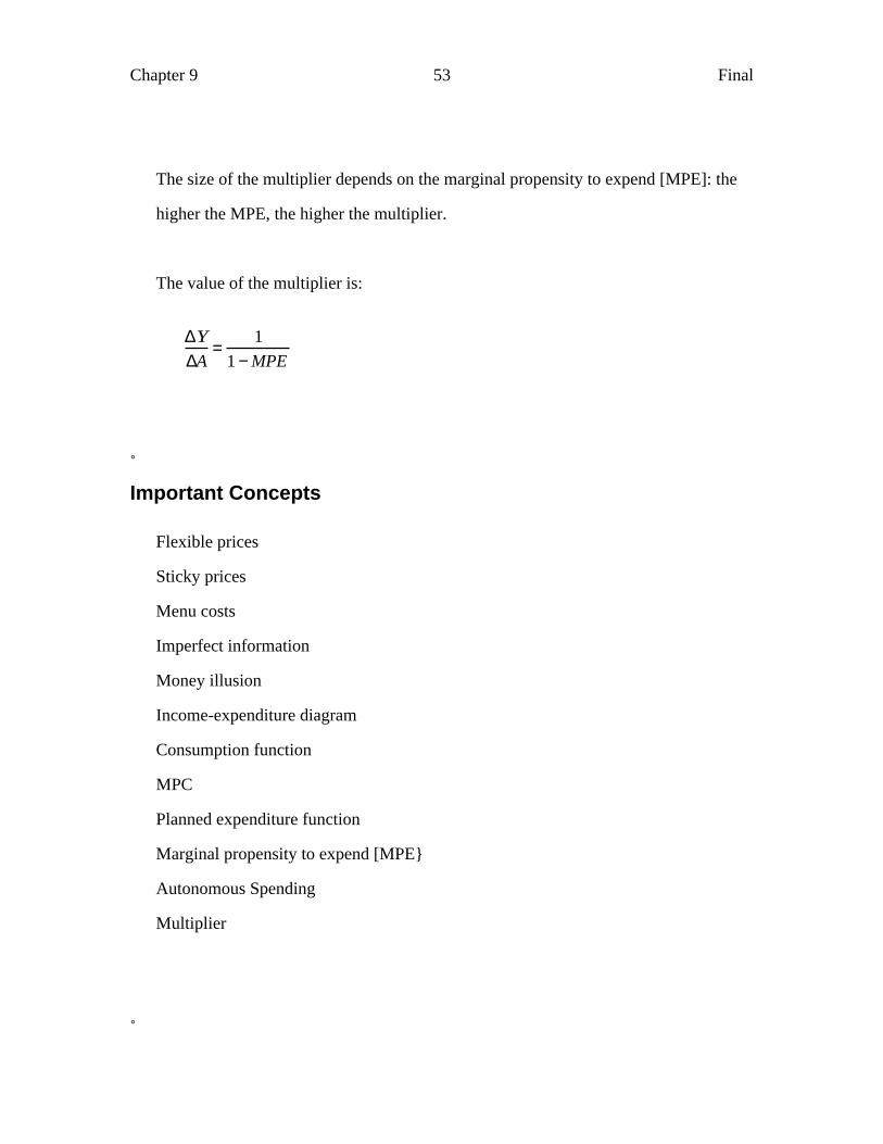
The size of the multiplier depends on the marginal propensity to expend [MPE]: the
higher the MPE, the higher the multiplier.
The value of the multiplier is:
∆Y
∆A=
1
1 − MPE
Important Concepts
Flexible prices
Sticky prices
Menu costs
Imperfect information
Money illusion
Income-expenditure diagram
Consumption function
MPC
Planned expenditure function
Marginal propensity to expend [MPE}
Autonomous Spending
Multiplier

Chapter 9 54 Final
Analytical Exercises
1. Describe, in your own words, the factors that determine the slope of the planned
expenditure curve.
2. Suppose that government purchases increase by $100 billion, but that there are no
other changes in economic policy or the economic environment.
a. What effect does this increase in government purchases have on the location of
the planned-expenditure line?
b. What effect does this increase in government purchases have on the planned
expenditure function?
c. What effect does this increase in government purchases have on the equilibrium
level of aggregate demand, national income, and real GDP?
3. Consider an economy in which prices are sticky, the marginal propensity to consume
out of disposable income Cy is 0.6, the tax rate t is 0.25, and the share of national income
spent on imports IMy is 20 percent.
a. Suppose that total autonomous spending is $6 trillion. Graph planned
expenditure as a function of total national income.
b. Determine the equilibrium level of national income and real GDP.
c. What is the value of the multiplier?
d. Suppose that total autonomous spending increases by $100 billion to $6.1
trillion. What happens to the equilibrium level of national income and real GDP,
Y?

Chapter 9 55 Final
4. Suppose that prices are sticky, the marginal propensity to consume out of disposable
income Cy is 0.9. Suppose further that the economy is closed--the share of national
income spend on imports is zero--and that the tax rate is 12.5 percent.
a. What is the marginal propensity to expend [MPE]?
b. What is the value of the multiplier?
c. What level of autonomous spending would be needed to attain a level of
equilibrium aggregate demand equal to $10 trillion?
5. Classify the following set of changes into two groups: those that increase equilibrium
real GDP, and those that decrease real GDP.
An increase in consumers' desire to spend today.An increase in interest rates overseas.A decline in foreign exchange speculators' confidence in the value of the homecurrency.A fall in real GDP overseas.An increase in government purchases.An increase in managers' expectations of the future profitability of investments.An increase in the tax rate.
6. Can you think of a price that is clearly sticky in the short run, yet clearly flexible in the
long run?
7. Suppose that the government wishes (for good reasons) to increase the equilibrium
level of real GDP by $500 billion. How would you suggest that the government go about
figuring out how to accomplish this goal?

Chapter 9 56 Final
Policy-Relevant Exercises [to be updated every year…]
1. In Washington today some people are arguing that the best measure of the federal
government's short-run impact on the economy is the government surplus: tY-G, where t
is the total tax rate. Others argue that the best measure is the non-Social-Security surplus
t'Y - G, where t' is the total tax rate minus the 8 percent or so of national income collected
in Social Security taxes plus the 6 percent or so of national income paid out in Social
Security benefits.
a. Break autonomous spending down into two parts, other autonomous spending
A' and government spending G. Find an algebraic expression for the level of real
GDP as a function of the multiplier and of these two components of autonomous
spending.
b. In your answer for (a), replace the multiplier with the appropriate function of its
determinants--the MPC, the tax rate, and the import share IMy.
c. Determine the difference between the short-run level of real GDP with
government spending equal to G and the tax rate equal to t, and the short-run level
of real GDP with government spending equal to zero and the tax rate equal to t.
d. Determine the difference between the short-run level of real GDP with
government spending equal to G and the tax rate equal to t, and the short-run level
of real GDP with government spending equal to G and the tax rate equal to 0.
e. What do you now think that the best measure of the impact of federal
government taxing and spending is on the level of GDP in the short run? Why?

Chapter 9 57 Final
2. Suppose that the economy is at its full-employment level of output of $8 trillion, with
government purchases equal to $1.6 trillion, the net tax rate equal to 20%, and the budget
in balance.
a. Suppose that adverse shocks to consumption and investment lead real GDP to
fall to $7.5 trillion. What is the level of taxes collected? What is the government's
budget deficit?
b. Suppose that favorable shocks to consumption and investment lead real GDP to
rise to $9.5 trillion. What is the level of taxes collected? What is the government's
budget balance?
c. Most economists like to calculate a "full employment budget balance" equal to
government purchases minus what tax collections would be if the economy were
at full employment, and to take that "full employment budget balance" as their
summary measure of the short-run effect of government taxes and spending on the
level of real GDP. What advantages does such a full-employment budget measure
have over the actual budget as a measure of economic policy? What
disadvantages does it have?
3. Suppose that the economy is short of its full-employment level of GDP, $8 trillion, by
$500 billion, with the MPC out of disposable income equal to 0.6, the import share IMy
equal to 0.2, and the tax rate t equal to 25%.
a. Suppose the government wants to boost real GDP up to full employment by
cutting taxes. How large a cut in the tax rate is required to boost real GDP to full
employment? How large a cut in total tax collections is produced by this cut in the
tax rate?

Chapter 9 58 Final
b. Suppose the government wants to boost real GDP up to full employment by
increasing government spending. How large an increase in government spending
is required to boost real GDP to full employment?
c. Can you account for any asymmetry between the answers to (a) and (b)?
4. Think about the four possible source of price stickiness mentioned in this chapter:
money illusion, "fairness" considerations, misperceptions of price changes, and menu
costs. What have you read or seen in the past two months that strike you as examples of
any of these four phenomena? Which of the four strikes you as most likely to be the most
important?
5. What changes in the economy's institutions can you think of that would diminish price
stickiness and increase price flexibility? What advantage in terms of the size of the
business cycle would you expect to follow from such changes in institutions? What
disadvantages do you think that such institutional changes might have?