part scale modeling of laser powder bed fusion ... - cism.it
TRANSCRIPT

LLNL-PRES-826837This work was performed under the auspices of the U.S. Department of Energy by Lawrence Livermore National Laboratory under contract DE-AC52-07NA27344. Lawrence Livermore National Security, LLC
Part Scale Modeling of Laser Powder Bed Fusion Additive Manufacturing
Neil HodgeMethods Development GroupLLNL
CISM 2021, C2119, “Metal Additive Manufacturing”

LLNL-PRES-8268373
• Day 1: Physical effects relevant for part-scale thermo-solid
mechanics in metal AM, and numerical methods
• Day 2: Numerical methods continued, constitutive models and
modeling techniques, and prediction of residual stresses and
dimensional warping
• Day 3: Improving accuracy of numerical models by handling the
multiscale nature of the problem
Overview

LLNL-PRES-8268374
• Introduction/Scope and Caveats
• Motivation
• Analytical models
• Strong forms: heat transfer, solid mechanics
• Weak form: heat transfer
• Modeling techniques and numerical methods
• Discrete weak form, time integration
• Nonlinear solution
• Multiphysics solution
Day 1 Contents

LLNL-PRES-8268375
• Me• Ph.D., UC Berkeley, 2011
• Solid mechanics and finite elements• GSI multiple classes, including continuum mechanics and graduate level finite elements
• MDG@LLNL, 2011-present• AM research, 2012-present
Introduction

LLNL-PRES-8268376
• Me• Ph.D., UC Berkeley, 2011
• Solid mechanics and finite elements• GSI multiple classes, including continuum mechanics and graduate level finite elements
• MDG@LLNL, 2011-present• AM research, 2012-present: pure luck . . .
Introduction

LLNL-PRES-8268377
• Me• Ph.D., UC Berkeley, 2011
• Solid mechanics and finite elements• GSI multiple classes, including continuum mechanics and graduate level finite elements
• MDG@LLNL, 2011-present• AM research, 2012-present: pure luck . . .
• Methods Development Group• Originated by G. Goudreau and J. Hallquist in mid- to late-1970s• Roots in solid mechanics, but now working in heat and mass transfer as well• Currently develops/maintains two massively parallel finite element codes, one explicit,
one implicit• AM work has been performed in the implicit code (“Diablo”)
Introduction

LLNL-PRES-8268378
• Process: laser power bed fusion
• Problem: “part” scale (so no explicit representation of powder particles or melt pools, and no microstructure)
• Modeling: implicit finite elements
• High accuracy
• I will inevitably have to skip some of the details . . .
Scope and Caveats

LLNL-PRES-8268379
• Process: laser power bed fusion
• Problem: “part” scale (so no explicit representation of powder particles or melt pools, and no microstructure)
• Modeling: implicit finite elements
• High accuracy
• I will inevitably have to skip some of the details . . .
• Acknowledgements:• R. Ferencz, R. Ganeriwala, J. Solberg, and W. King
• And numerous others . . .
Scope and Caveats

LLNL-PRES-82683710
• Designers hear the promises . . .
Motivation

LLNL-PRES-82683711
• Designers hear the promises . . .
• But not everything can be built, or at least not easily
Motivation

LLNL-PRES-82683712
• Design failures
• Stress state . . .
Motivation

LLNL-PRES-82683713
• Design failures
• Stress state => self-explanatory
• Final configuration . . .
Motivation
LLNL-PRES-82683714
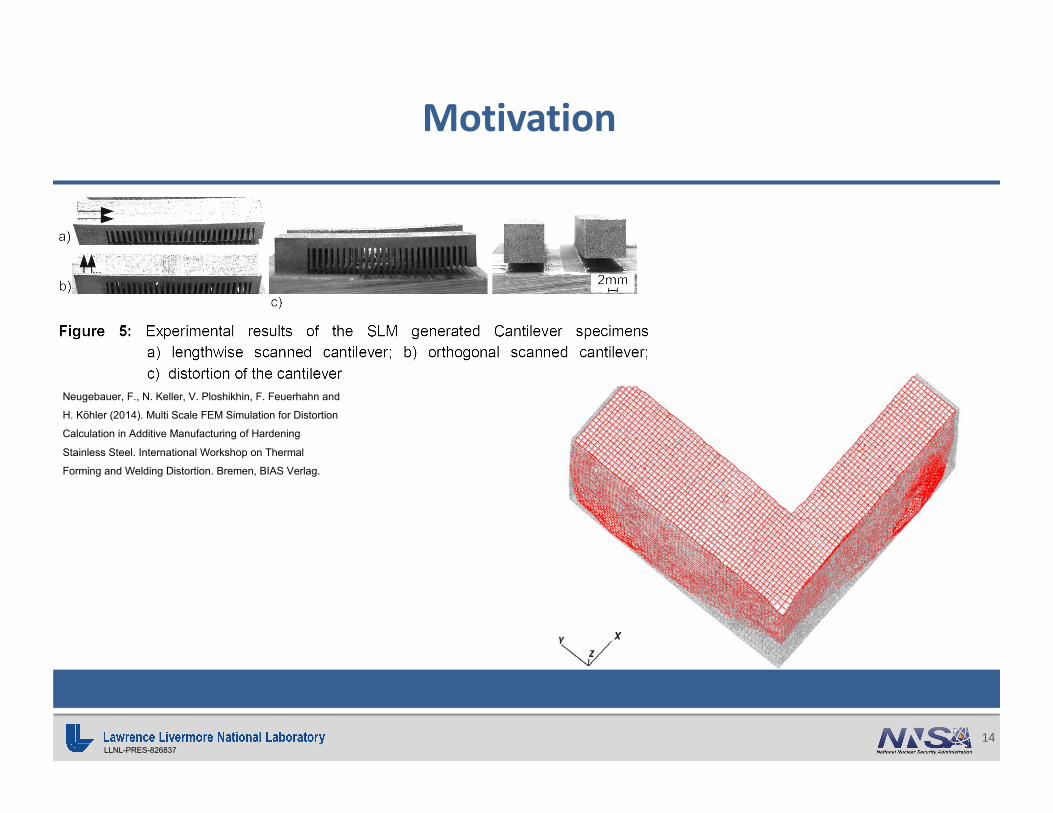
Motivation
Neugebauer, F., N. Keller, V. Ploshikhin, F. Feuerhahn and
H. Köhler (2014). Multi Scale FEM Simulation for Distortion
Calculation in Additive Manufacturing of Hardening
Stainless Steel. International Workshop on Thermal
Forming and Welding Distortion. Bremen, BIAS Verlag.

LLNL-PRES-82683715
• Design failures
• Stress state => self-explanatory
• Final configuration => stresses
Motivation

LLNL-PRES-82683716
• Design failures
• Stress state => self-explanatory
• Final configuration => stresses
• Build failures
• Lack of fusion, or porosity/keyholing . . .
Motivation

LLNL-PRES-82683717
Motivation
R. Cunningham, C. Zhao, N. Parab, C. Kantzos, J. Pauza,
K. Fezzaa, T. Sun, A. D. Rollett, “Keyhole threshold and
morphology in laser melting revealed by ultrahigh-speed x-
ray imaging”, Science, 363, 2019

LLNL-PRES-82683718
• Design failures
• Stress state => self-explanatory
• Final configuration => stresses
• Build failures
• Lack of fusion, or porosity/keyholing => heat transfer
• Cracking . . .
Motivation

LLNL-PRES-82683719
Motivation
• 316L

LLNL-PRES-82683720
Understanding the part scale behavior requires heat transfer and solid mechanics
• Design failures
• Stress state => self-explanatory
• Final configuration => stresses
• Build failures
• Lack of fusion, or porosity/keyholing => heat transfer
• Cracking => stresses
• Solid mechanics results also dependent on other thermal features
• Laser scan path . . .
Motivation

LLNL-PRES-82683721
Motivation

LLNL-PRES-82683722
Balance of thermal energy, strong form
!"$ = −div * + ,, in Ω$ 0!, 1 = 2$, on 0! ∈ Γ!6 0", 1 = 7* 8 9, on 0" ∈ Γ"$ 0, 0 = $#, on Ω ∪ <Ω
where <Ω is the boundary of Ω, and <Ω = Γ!⨃Γ"
Analytical Model

LLNL-PRES-82683723
• Constitutive relation (Fourier’s Law):
* = −> grad $
• Associated moving boundary problem for phase change (Stephan-Neumann)
$ 0$, 1 = $$, on 0$ ∈ Γ$
>%<$%<0
− >&<$&<0
8 9 = B!<0$<1
8 9, on 0$ ∈ Γ$
where Γ$ is the phase interface, and B is the latent heat
Analytical Model

LLNL-PRES-82683724
• Balances of mass and linear momentum
! = ! div C, in Ω! 0, 0 = !#, on Ω ∪ <Ω
!C = div D + !E, in ΩF 0', 1 = 7F, on Γ'G 0(, 1 = G, on Γ(
F 0, 0 = F#, on Ω ∪ <ΩG 0, 0 = G#, on Ω ∪ <Ω
• Balance of angular momentum as usual . . . D = D!
Analytical Model

LLNL-PRES-82683725
residuals: !"$ = − div * + , in Ω, * 8 9 0(, 1 = 26, on Γ",
weighted residual:
I)J) !"$ + div * − , KΩ +I
*!J" −* 8 9 + 26 KΓ = 0
Galerkin => J) = J" = J :
I)
J!"$ + w6+,+ −J, KΩ +I*!
−J* 8 9 + J26 KΓ = 0
Analytical Model

LLNL-PRES-82683726
Integration by parts + divergence theorem:
I)
J!"$ − J,+6+ −J, KΩ +I-)J6+M+ KΓ
+I*!
−J* 8 9 + J26 KΓ = 0
Analytical Model

LLNL-PRES-82683727
Integration by parts + divergence theorem:
I)
J!"$ − J,+6+ −J, KΩ +I-)J6+M+ KΓ
+I*!
−J* 8 9 + J26 KΓ = 0
Analytical Model

LLNL-PRES-82683728
Integration by parts + divergence theorem:
I)
J!"$ − J,+6+ −J, KΩ +I-)J6+M+ KΓ
+I*!
−J* 8 9 + J26 KΓ = 0
Analytical Model

LLNL-PRES-82683729
Integration by parts + divergence theorem:
I)
J!"$ − J,+6+ −J, KΩ + I*"J6+M+ KΓ +I
*!J6+M+ KΓ
+I*!
−J* 8 9 + J26 KΓ = 0
Analytical Model
Dirichlet Neumann

LLNL-PRES-82683730
Integration by parts + divergence theorem:
I)
J!"$ − J,+6+ −J, KΩ + I*"J6+M+ KΓ +I
*!J6+M+ KΓ
+I*!
−J* 8 9 + J26 KΓ = 0
Combining boundary terms, and assume J = 0 on Γ!:
I)
J!"$ − J,+6+ −J, KΩ +I*!J26 KΓ = 0
Analytical Model
Dirichlet Neumann

LLNL-PRES-82683731
Analytical ”weak form”: Find $ ∈ N, such that, for all J ∈ O,
I)
J!"$ − J,+6+ −J, KΩ +I*!J26 KΓ = 0
where
N = $ ∈ B% Ω | $ = 2$ on Γ! ,
O = J ∈ B% Ω | J = 0 on Γ!
Solid mechanics weak form is derived more or less identically
Analytical Model
LLNL-PRES-82683732
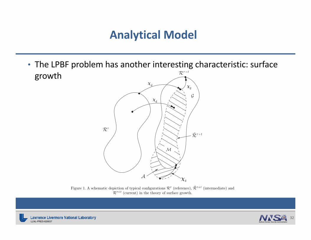
• The LPBF problem has another interesting characteristic: surface growth
148149150151152153154155156157158159160161162163164165166167168169170171172173174175176177178179180181182183184185186187188189190191192193194195196
ARTICLE IN PRESS4 N. Hodge and P. Papadopoulos
g
gd
d
Figure 1. A schematic depiction of typical configurations Rt (reference), Rt+t (intermediate) andRt+t (current) in the theory of surface growth.
Once the boundary vRt+t is determined, the region Rt+t occupied by the bodyat time t + t is defined by
Rt+t = int(vRt+t), (2.6)
where ‘int’ denotes the interior of an orientable surface. The regions vRt+t andvRt+t defined by means of the decomposition (2.5) are depicted in figure 1.
The decomposition (2.5) is an essential feature of the proposed theory. Indeed,this decomposition enables the definition of the region Rt+t for bodies undergoingsurface growth. As will be established later in this section, the decomposition (2.5)also permits the distinction between growth regions and material regions in thetime interval (t, t + t]. Note that the order of the composition of cg and cd isimportant in the ensuing developments. This is because admitting that the bodyfirst undergoes a pure deformation followed by growth enables the definition of themaps cd and cg on vRt and vRt+t , which are simple to motivate. Specifically,one may take cd to apply to the body in (t, t + t] by assuming that growthis suppressed. This is followed by cg, which effects all surface growth withoutdeformation. The alternative of imposing surface growth first on the configurationvRt, while not in any sense erroneous, is conceptually less appealing. Indeed, ifsurface growth/resorption were to be effected first, then boundary conditionswould need to be enforced on material points that come to existence (or reachthe boundary of the body) simultaneously with the application of these boundaryconditions.
Proc. R. Soc. A (2010)
Analytical Model

LLNL-PRES-82683733
• Surface growth traits
• Points come into existence at different times, at the surface of an existing configuration
• The intuitive notion of a reference configuration is discontinuous
• The displacements are also discontinuous
• Implication: Incremental formulation eases handling of surface growth
148149150151152153154155156157158159160161162163164165166167168169170171172173174175176177178179180181182183184185186187188189190191192193194195196
ARTICLE IN PRESS4 N. Hodge and P. Papadopoulos
g
gd
d
Figure 1. A schematic depiction of typical configurations Rt (reference), Rt+t (intermediate) andRt+t (current) in the theory of surface growth.
Once the boundary vRt+t is determined, the region Rt+t occupied by the bodyat time t + t is defined by
Rt+t = int(vRt+t), (2.6)
where ‘int’ denotes the interior of an orientable surface. The regions vRt+t andvRt+t defined by means of the decomposition (2.5) are depicted in figure 1.
The decomposition (2.5) is an essential feature of the proposed theory. Indeed,this decomposition enables the definition of the region Rt+t for bodies undergoingsurface growth. As will be established later in this section, the decomposition (2.5)also permits the distinction between growth regions and material regions in thetime interval (t, t + t]. Note that the order of the composition of cg and cd isimportant in the ensuing developments. This is because admitting that the bodyfirst undergoes a pure deformation followed by growth enables the definition of themaps cd and cg on vRt and vRt+t , which are simple to motivate. Specifically,one may take cd to apply to the body in (t, t + t] by assuming that growthis suppressed. This is followed by cg, which effects all surface growth withoutdeformation. The alternative of imposing surface growth first on the configurationvRt, while not in any sense erroneous, is conceptually less appealing. Indeed, ifsurface growth/resorption were to be effected first, then boundary conditionswould need to be enforced on material points that come to existence (or reachthe boundary of the body) simultaneously with the application of these boundaryconditions.
Proc. R. Soc. A (2010)
Analytical Model

LLNL-PRES-82683734
• We calculate the solution with finite elements, as follows:
Q./ =R0
1#$S0/ TQ0/ = S%/ S&/ ⋯
TQ%TQ&⋮
= W/XF/
J./ =R0
1#$S0/XJ0/ = W/XY/
where 8 are the nodal quantities
Numerical Methods
LLNL-PRES-82683735
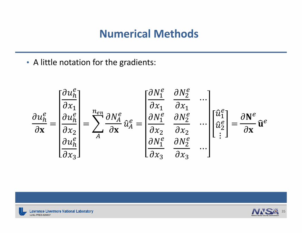
• A little notation for the gradients:
<Q./
<0=
<Q./
<[%<Q./
<[&<Q./
<[2
=R0
1#$ <S0/
<0TQ0/ =
<S%/
<[%<S&/
<[%⋯
<S%/
<[&<S&/
<[&⋯
<S%/
<[2<S&/
<[2⋯
TQ%/
TQ&/⋮
=<W/
<0XF/
Numerical Methods

LLNL-PRES-82683736
Discrete weak form:
I)
WX\ !" W]D −<W<0
X\ 8 −^<W<0
]D − WX\ , KΩ
+I*!
WX\ 26 KΓ = 0
X\3 _
`
∫) W3!"W]D − -4-5
3−^ -4-5
]D − W3, KΩ +
∫*! W326 KΓ = 0, for all X\
Numerical Methods

LLNL-PRES-82683737
Now, over individual elements:
R/b
c
I)#
W/ 3!"W/ ]D/ −<W/
<0
3−^
<W/
<0]D/ − W/ 3, KΩ
+I*!#W326 KΓ = 0
Numerical Methods
LLNL-PRES-82683738
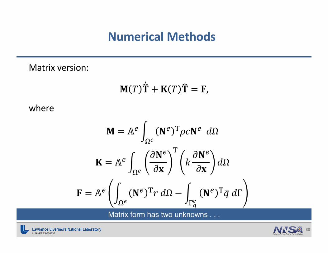
Matrix version:
d $ ]D + e $ ]D = f,
where
d = g/I)#
W/ 3!"W/ KΩ
e = g/I)#
<W/
<0
3^<W/
<0KΩ
f = g/ I)#
W/ 3, KΩ −I*!#
W/ 326 KΓ
Matrix form has two unknowns . . .
Numerical Methods

LLNL-PRES-82683739
• Matrix version at time M + 1:
d]D16% +e]D16% = f16%,
where
$16% = $1 + K1 1 − i $1 + i$16% ,
(which holds equally well for the nodewise values)
• States at time M known, so two equations and two unknowns
• Use any desired nonlinear solution method for top equation
Numerical Methods

LLNL-PRES-82683740
• Newton-Raphson is the canonical nonlinear solution:
]D16%76% = ]D16%7 + ∆]D16%7 ,
where the superscript is the nonlinear iteration, and ∆]D16%7 is called the increment of the solution
• How to calculate ∆]D16%7 ? Residual of the matrix form from preceding slide:
k = d]D16% +e]D16% − f16% = l
Numerical Methods

LLNL-PRES-82683741
• Calculate the linear portion of k in the direction of the solution increment:
ℒ k, ∆]D16%7 = k ]D16%7 +D83k ]D16%7 ∆]D16%7 = l,
where D83k is the Fréchet derivative of k with respect to ]D16%, and is often referred to colloquially in the solids community as the “stiffness” (and denoted by the notation e, and less frequently,
o-9-8: )
• Rearrange . . .
∆]D16%7 = − D83k ]D16%7 ;%k ]D16%7
Numerical Methods

LLNL-PRES-82683742
• The analogous system of equation for solids would be:
dXF16% + rXF16% +eXF16% = f,
where time integration is handled by Newmark:
F16% = F1 + K1 1 − s F1 + sF16%
F16% = F1 + K1 F1 + K1&12− i F1 + i F16%
Numerical Methods

LLNL-PRES-82683743
• Staggered multiphysics:
Initialize: $16% = $1, Q16% = Q1
Numerical Methods

LLNL-PRES-82683744
• Staggered multiphysics:
Initialize: $16% = $1, Q16% = Q1
Iteration 1/thermal: Hold Q16% fixed, update $16%
Iteration 1/solid: Hold $16% fixed, update Q16%
Numerical Methods

LLNL-PRES-82683745
• Staggered multiphysics:
Initialize: $16% = $1, Q16% = Q1
Iteration 1/thermal: Hold Q16% fixed, update $16%
Iteration 1/solid: Hold $16% fixed, update Q16%
Iteration 2/thermal: Hold Q16% fixed, update $16%
…
Until convergence
Numerical Methods

LLNL-PRES-82683746
• Convergence for staggered problems:
• Physics 1: regular single-physics convergence for multi-physics iteration n+1• Physics 2: regular single-physics convergence for multi-physics iteration n+1• …• Physics p: regular single-physics convergence for multi-physics iteration n+1
Numerical Methods

LLNL-PRES-82683747
• Convergence for staggered problems:
• Physics 1: regular single-physics convergence for multi-physics iteration n+1• Physics 2: regular single-physics convergence for multi-physics iteration n+1• …• Physics p: regular single-physics convergence for multi-physics iteration n+1• After each individual physics complete for iteration n+1, check the
following:• For each physics <!"#$, check that
=%&' − =% < @(!"#$ ,that is, that the solution for each physics has not changed “much” between the current and the previous iterations
Numerical Methods
LLNL-PRES-82683748
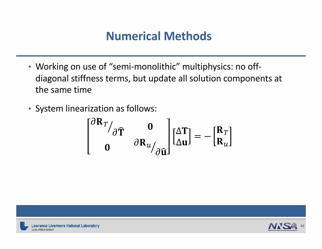
• Working on use of “semi-monolithic” multiphysics: no off-diagonal stiffness terms, but update all solution components at the same time
• System linearization as follows:
o<k!<]D l
l o<k'<XF
∆D∆F = − k!
k'
Numerical Methods

LLNL-PRES-82683749
• Working on use of “semi-monolithic” multiphysics: no off-diagonal stiffness terms, but update all solution components at the same time
• System linearization as follows:
o<k!<]D l
l o<k'<XF
∆D∆F = − k!
k'
• Expectation: same solution, faster convergence
A natural step on the way to fully-ish monolithic solutions
Numerical Methods

LLNL-PRES-82683750
• The next step . . . “monolithic” solutions
o<k!<]D
o<k!<XF
o<k'<]D
o<k'<XF
∆D∆F = − k!
k'
Numerical Methods

LLNL-PRES-82683751
• The next step . . . “monolithic” solutions
o<k!<]D
o<k!<XF
o<k'<]D
o<k'<XF
∆D∆F = − k!
k'
Numerical Methods

LLNL-PRES-82683752
• The next step . . . “monolithic” solutions
o<k!<]D
o<k!<XF
o<k'<]D
o<k'<XF
∆D∆F = − k!
k'
• Unlikely that !!"! !#$ (strain/deformation heating) will ever contribute much . . . So, most likely “monolithic” formulation would be
o<k!<]D l
o<k'<]D
o<k'<XF
∆D∆F = − k!
k'
Numerical Methods
