part v correlation analysis & simple regression dr. stephen h. russell weber state university

Part VPart VCorrelation Analysis &

Simple Regression

Dr. Stephen H. RussellDr. Stephen H. Russell

Weber State UniversityWeber State University

5.2

Correlation Analysis Correlation Analysis

Shows the direction and the strength of the linear relationship between two variables.

Informal analysis is done with a scatter diagram

Formal analysis is done by computing a sample correlation coefficient (r) and an associated P-value.

5.3

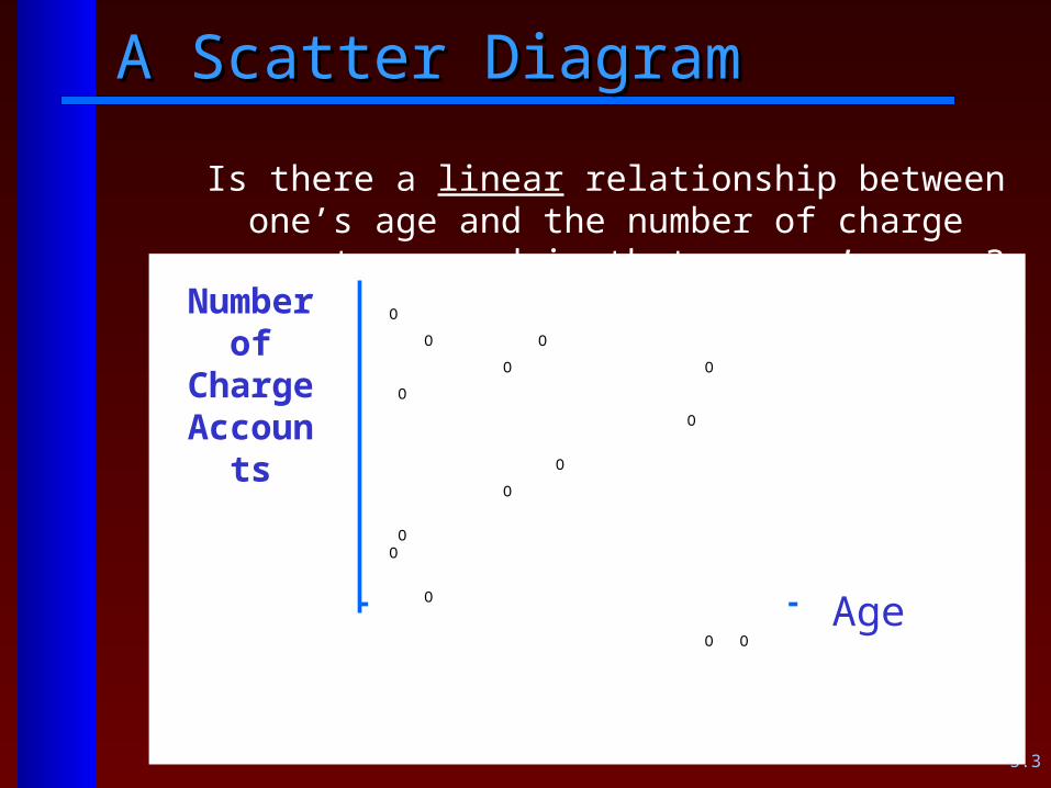
A Scatter DiagramA Scatter Diagram

Age

Number of

Charge Accounts

O

O O

O O

O

O

O

O

O O

O

O O

Is there a linear relationship between one’s age and the number of charge accounts opened in that person’s name?

5.4

The Correlation CoefficientThe Correlation Coefficient

Must be between +1.0 and – 1.0

The sign shows the direction of the relationship; the absolute value of the number shows the strength

The population correlation coefficient

is (rho)

The sample correlation coefficient is r

5.5

Correlation AnalysisCorrelation Analysis A single number that measures the strength

of association between two variables.

In which diagram would r = 0? = +1.0? = +.70? What would a diagram look like for r = -1.0?

5.6

Correlation AnalysisCorrelation Analysis

Rarely will we get an r = 0.00 from sample information even if there is no correlation between the two variables.

Therefore, we test these hypotheses:

HO: = 0

HA: 0

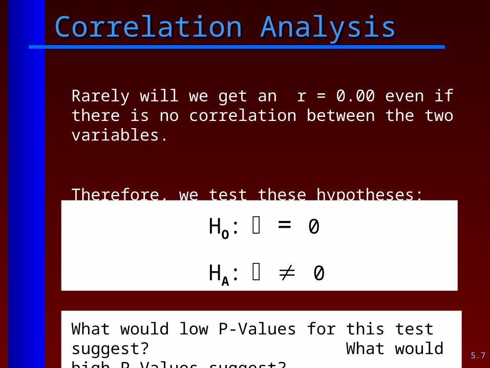
5.7

Correlation AnalysisCorrelation Analysis

Rarely will we get an r = 0.00 even if there is no correlation between the two variables.

Therefore, we test these hypotheses:

HO: = 0

HA: 0

What would low P-Values for this test suggest? What would high P-Values suggest?

5.8

ExampleExample

I wonder if there is correlation between a student’s age and his/her GPA. I collect these data:

AGE GPA

19 3.3 22 3.0 24 2.7 18 3.95 30

2.9 20 2.5

Let’s use MINITAB to plot the data with GRAPH PLOT command, compute the sample correlation coefficient, and make a decision on the statistical significance of our sample r

5.9

Consider these MINITAB ExamplesConsider these MINITAB Examples

Is the sample correlation coefficient sufficiently different from zero to conclude linear correlation between:

1. Gross Vehicle Weight and Gas Mileage?

2. Number of sales calls made by a copy machine salesperson and copiers sold?

3. High School GPA and College GPA?

5.10

Simple Regression AnalysisSimple Regression Analysis

Similar to Correlation Analysis but considerably more sophisticated

Regression Analysis postulates causation

Regression analysis allows us to develop an equation that explains or estimates the value of one variable (Y) in terms of another variable (X)

5.11


Similar to Correlation Analysis but considerably more sophisticated

Regression Analysis postulates causation

Regression analysis allows us to develop an equation that explains or estimates the value of one variable (Y) in terms of another variable (X); i.e. movements in X cause movements in Y.

5.12

An example regression equation:An example regression equation:

Y = f(X)

Selling price of a home = f(Square Footage)

Using sample information, we might develop this equation:

bXaYx ˆ

XYx 39.8715975ˆ

5.13


Y = f(X)

Selling price of a home = f(Square Footage)

Using sample information, we might develop this equation:

bXaYx ˆ

XYx 39.8715975ˆ

Mathematically, what is “b” in this equation?

5.14


XYx 39.8715975ˆ

A home of 2200 square feet would be estimated to cost:

$15,975 + $87.39(2200) = $208,233

5.15


Four Important Concepts

5.16

I. Independent vs. Dependent Variables I. Independent vs. Dependent Variables

Y is a function of X or Y=f(X)

X is the Independent Variable (also called the explanatory variable, or predictor variable)

Variable whose value is known

Y is the Dependent Variable (or the response variable)

Variable whose value is unknown; is explained with the help of another variable

5.17

ExampleExample

S’pose I want to build a regression equation that explains or predicts sales in my organization. My experience suggests a contributing factor is our advertising budget.

What has to be Y (the dependent variable)?

What has to be X (the independent or explanatory variable)?

5.18

II. Deterministic vs. Stochastic RelationshipsII. Deterministic vs. Stochastic Relationships

Deterministic relationship: value of Y is uniquely determined whenever the value of X is specified; only one Y exists for each X

A precise and fixed mathematical relationship

Stochastic relationship: imprecise in the sense that many possible values of Y can be associated with any one value of X

A statistical relationship (involving probability or uncertainty); not a precise but an estimated relationship

5.19

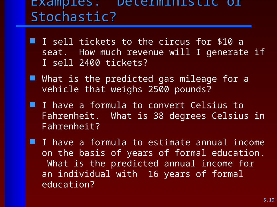
Examples: Deterministic or Stochastic?Examples: Deterministic or Stochastic?

I sell tickets to the circus for $10 a seat. How much revenue will I generate if I sell 2400 tickets?

What is the predicted gas mileage for a vehicle that weighs 2500 pounds?

I have a formula to convert Celsius to Fahrenheit. What is 38 degrees Celsius in Fahrenheit?

I have a formula to estimate annual income on the basis of years of formal education. What is the predicted annual income for an individual with 16 years of formal education?

5.20

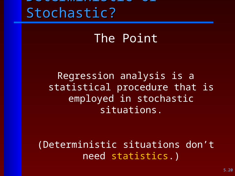
Deterministic or Stochastic?Deterministic or Stochastic?

The Point

Regression analysis is a statistical procedure that is employed in stochastic situations.

(Deterministic situations don’t need statistics.)

5.21

III. Direct vs Inverse RelationshipsIII. Direct vs Inverse Relationships

If the values of the dependent variable, Y, increase with larger values of the independent variable, X, the variables are said to have a direct relationship: slope of the regression line (b) is positive .

If the values of the dependent variable, Y, decrease with larger values of the independent variable, X, the variables are said to have an inverse relationship: slope of the regression line (b) is negative.

5.22

IV. “Causation” in Regression AnalysisIV. “Causation” in Regression Analysis

Regression “postulates” causation but it cannot prove causation.

For example, does increased R&D spending increase profits or do increased profits lead to increased R&D spending?

What if I find a statistically significant and positive relationship between the amount of gray hair a man has and his blood pressure. Do increased amounts of gray hair cause higher blood pressure?

5.23

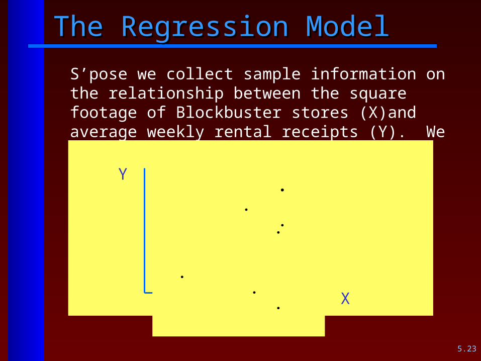
The Regression ModelThe Regression Model

S’pose we collect sample information on the relationship between the square footage of Blockbuster stores (X)and average weekly rental receipts (Y). We get these results:

. . . . . . .

Y

X

5.24


The regression line of the form

generates a “line of best fit.”The regression line (of the form

. . . . . . .

Y

X

bXaYx ˆ

5.25


For each “X” in our sample (the square footage of a Blockbuster store), notice we have two “Y’s”—the observed “Y” (the dot) and the predicted Y or (the point on the red line). NOTE: MINITAB refers to the predicted Y’s as “Fits”)

. . . . . . .

Y

X

xY

Predicted Y for X = 3000 sq ft

3000

Observed Y for the 3000 sq ft store

5.26


The difference between the observed Y and the predicted Y is called the error term or the residual: ex = Yx –

. . . . . . .

Y

X

xY


3000


Error term

5.27

The Method of Least SquaresThe Method of Least Squares

Error term: ex = Yx –

For observations above the regression line, error terms are positive. For observations below the regression line, error terms are negative.

. . . . . . .

Y

X

xY


3000


5.28

True or False?True or False?

xxx eYY ˆ

True!

5.29


If the regression line is truly a “line of best fit,” what would the sum of the positive and negative error terms be?

. . . . . . .

Y

X


3000


5.30


Actually, three arithmetic characteristics occur in every calculated regression line: (1) The sum of the error terms is zero, (2) the regression line passes through the mean of the observed X’s; (3) the regression line passes through the

mean of the observed Y’s.

. . . . . . .

Y

X

The regression line passes through this point: the mean of the observed X’s and the mean of the observed Y’s

5.31


What is the precise definition of the error term?

The observed Y minus the predicted Y

What is another name for error terms?

The residuals

Residuals are important in Regression Analysis for many reasons. In fact, Regression Analysis is also called Least Squares (a term that relates to these residuals).

5.32

The Method of Least SquaresThe Method of Least Squares Regression, also called least squares regression, minimizes

the sum of the squares of the residuals (deviations between the line and the individual data plots). Hence it is called the method of least squares.

No other line could be drawn through the

observation points that would yield a lower value for the sum of

the squared residuals.

5.33

Doing Regression with MINITABDoing Regression with MINITAB

Lee County Sports Complex managers do a good job of predicting attendance at spring training games of the Minnesota Twins in Ft. Myers, FL. Bernie McFarland wants to be able to predict hot dog sales on the basis of attendance estimates he is given. Bernie collects hot dog sales and attendance data from a sample of 10 games.

What is the dependent variable? What is the independent variable?

Compute the regression equation and plot it.

5.34

Doing Regression with MINITABDoing Regression with MINITAB

The dependent variable (Y) is hot dog sales.

The Independent variable (X) is game attendance.

The least squares regression equation is:

. .Y XX 1 7 9 3 6 9 4

What is the error term for the second observation?

5.35

The True Regression lineThe True Regression line

Our regression equations are built upon sample information.

The “true” equation is never known. Symbolically it is:

X Y

bXaYx ˆ

We use sample information to obtain estimates for α and β

5.36

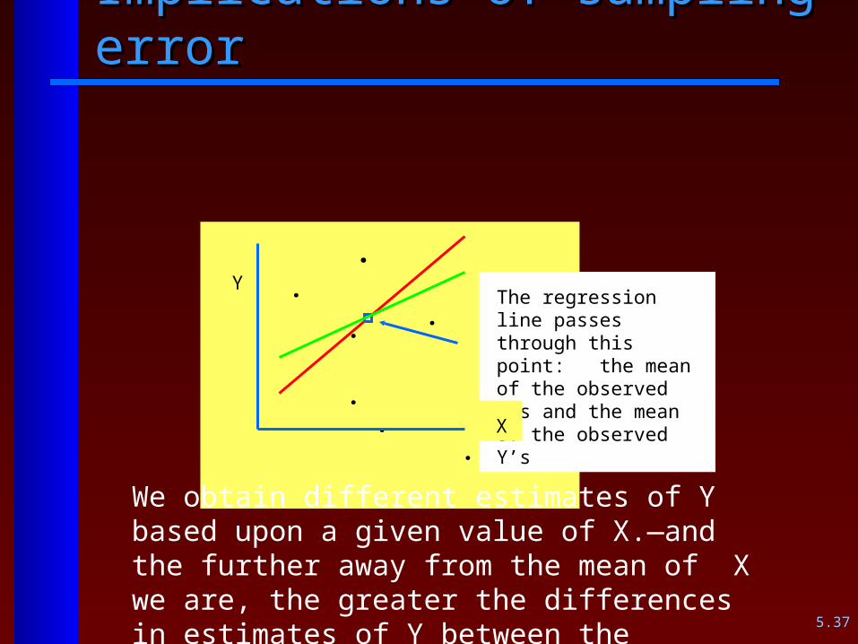
Implications of sampling errorImplications of sampling error

. . . . . . .


YY

X

The red line is one estimate of the true regression line. But another sample would give us other values for “a” and “b”. Notice the results of a second sample:

5.37

Implications of sampling errorImplications of sampling error

. . . . . . .


YY

X

We obtain different estimates of Y based upon a given value of X.—and the further away from the mean of X we are, the greater the differences in estimates of Y between the samples.

5.38

Regression DiagnosticsRegression Diagnostics

Y

xY

To know whether we can safely use our estimate of the true regression equation—that is whether we can rely upon our equation to make inferences about Y based upon values for X . . .

Three assumptions must be satisfied:

5.39

Assumptions for the Least Squares Regression Model

1. The error terms (residuals) associated with every value of X follow an approximate normal distribution.

2. The variance of the error terms is the same for each value of X. (Called the assumption of homoscedasticity.)

3. The errors are independent of each other.

5.40

To illustrate these assumptions . . .To illustrate these assumptions . . .

S’pose we build a regression model that postulates that home size is a function of a family’s annual income. The regression equation will give us the expected house size for a given level of income. However, in the population NOT EVERY family making $50,000 annual income will live in the same sized house. But the expected size of house will be given by

50Y

5.41

The distribution of Y’s for a given XThe distribution of Y’s for a given X

Picture this as a three-dimensional diagram of the distribution of Y values in the population for given X values.

Now let’s review the three assumptions

1740 sq ft

XY 6.24510ˆ

5.42

Assumptions for the Least Squares Regression Model

1. The error terms (residuals) associated with every value of X follow an approximate normal distribution.

2. The variance of the error terms is the same for each value of X. (Called the assumption of homoscedasticity.)

3. The errors are independent of each other.

5.43

Viewing plots of the residualsViewing plots of the residuals Assumption 1. The “Normal Plot” of the residuals

should approximate a straight line. Use the Anderson-Darling test to get a P-Value on the validity of Assumption 1.)

The null hypothesis in the Anderson-Darling test is “the data follow a normal distribution.”

Assumption 2. What we like to see is a “shotgun blast” appearance of the residuals. A sideways funnel appearance implies heteroscedasticity (violation of Assumption 2).

Assumption 3. A “snake appearance” (as opposed to a random appearance of the residuals implies autocorrelation (violation of Assumption 3.)

5.44

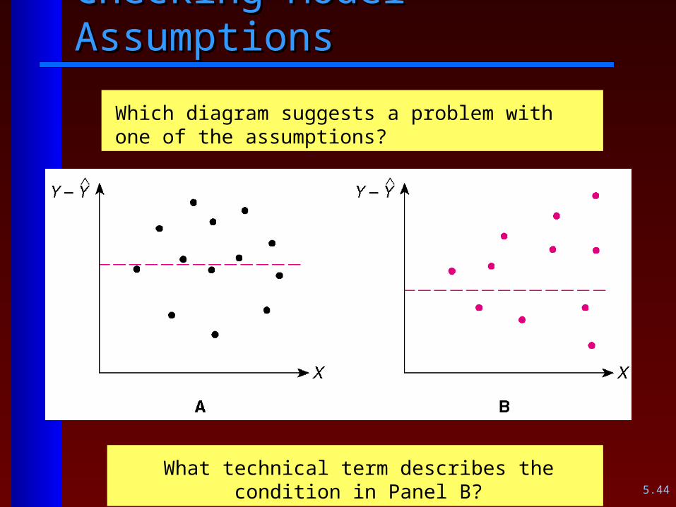
Checking Model AssumptionsChecking Model Assumptions

Which diagram suggests a problem with one of the assumptions?

What technical term describes the condition in Panel B?

5.45

Checking Model AssumptionsChecking Model Assumptions

This “snake” is bad news. What assumption is violated here?

The “snake” pattern in the residuals suggests autocorrelation

5.46

Regression AnalysisRegression Analysis The supreme purpose of regression analysis is to

model quantitatively the relationship between some dependent variable of interest (Y) and its explanatory variables.

Our goal is to find one or more “good” explanatory variables.

The quantitative relationship between Y and X is defined by the slope—b.

5.47

The “true” regression equationThe “true” regression equation

Implications of the sign of the true regression slope β:

β = 0 β > 0 β < 0

5.48

Hypothesis tests on Hypothesis tests on ββ

We must test these hypotheses to assess whether or not the “b” we obtained from sample information isstatistically different from zero.

Ho : 1 = 0 Ha : 1 0

Keep in mind that our regression equation is an estimate based upon sample information. We might, due to sampling error, obtain a non-zero slope (b) when β is actually zero.

Why are we as researchers hoping to reject the null?

5.49

Hypothesis tests on Hypothesis tests on ββ

Ho : 1 = 0 (X provides no information)Ha : 1 0 (X does provide information)

• If we reject the null, we keep “X” as an explanatory variable.

• If we fail to reject the null, we do reject “X” as an explanatory variable.

5.50

Hypothesis TestingHypothesis Testing

HO: μ = 0

HA: μ 0S.E.ns/

XXt

HO: = 0

HA : 0 bS

bbt

S.E.

Recall how we tested hypotheses on μ:

Similarly, we now test hypotheses on :

The t for tests on has n – 1 – k degrees of freedom, where k is

the number of explanatory variables (in this case “one”) .

5.51

Hypothesis TestingHypothesis Testing

HO: μ = 0

HA: μ 0S.E.ns/

XXt

HO: = 0

HA : 0 bS

bbt

S.E.

Recall how we tested hypotheses on μ:

Similarly, we now test hypotheses on :

MINITAB will give us a p value of this test of hypotheses.

5.52

Computing C.I.s on “b”Computing C.I.s on “b”

The denominator in the t calculation (the standard error of “b”) is employed to compute confidence interval estimates of the true population slope

b ± tα/2 · sb

where the t value is obtained from the t table (df = n-1-k) and sb1 is given by MINITAB regression results

5.53

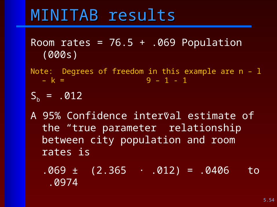
Here’s an example using MINITABHere’s an example using MINITAB

I want to examine the possible relationship between average room rates at three star lodgings and the population of the host city. Here’s the data I collect:

Room Rate City population in thousands

$119 986 $79 245 $74

88 $212 1938 $179

1482 $59106 $134

612 $164 1071 $123 84

5.54

MINITAB resultsMINITAB results

Room rates = 76.5 + .069 Population (000s)

Note: Degrees of freedom in this example are n – l – k = 9 – 1 - 1

Sb = .012

A 95% Confidence interval estimate of the “true parameter” relationship between city population and room rates is

.069 ± (2.365 · .012) = .0406 to .0974

5.55

Homework:Homework:

Problem Set 5

5.56

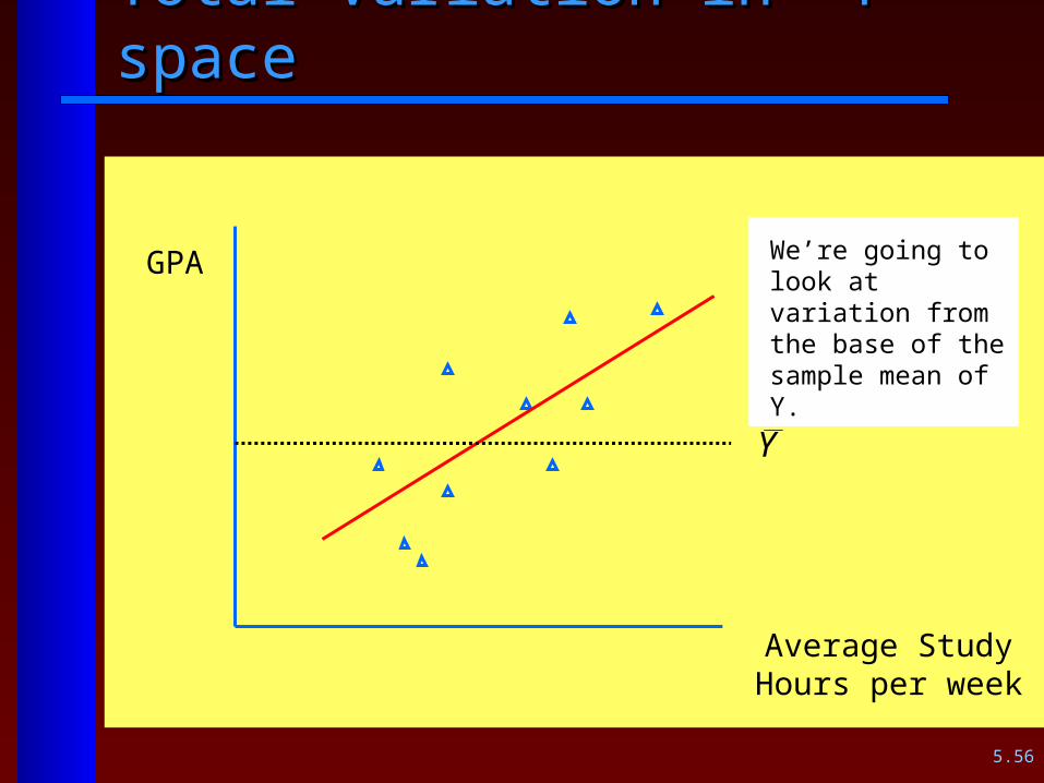
Total Variation in “Y space”Total Variation in “Y space”

Y

GPA

Average Study Hours per week

We’re going to look at variation from the base of the sample mean of Y.

5.57

Total VariationTotal Variation

Y

GPA


Why is this student’s GPA far above the average?

5.58


Y

GPA


What is her “predicted” GPA for her study hours?

5.59


Y

GPA


What is her “predicted” GPA for her study hours?

o

5.60


Y

GPA


Observed GPA for this particular student

o

Total Variation:

YYX

5.61


Y

GPA


Observed GPA for this particular student

o

The total variation from the mean GPA

can be broken into the explained and the

unexplained

5.62


Y

GPA


This student’s “predicted” GPA for her study hours?

o

Explained Variation:

YYX ˆ

5.63


Y

GPA


This student’s observed GPA for her study hours

o

Unexplained Variation:

XX YY ˆHer predicted GPA

5.64


Y

GPA


This student’s observed GPA for her study hours

o

Unexplained Variation:

XX YY ˆHer predicted GPA

What’s another name for Unexplained Variation?

5.65

Disaggregating the total variationDisaggregating the total variation

Y

GPA


o XY

XY

5.66

Variation in Y SpaceVariation in Y Space

Total Variation = Explained Variation + Unexplained Variation

)ˆ()ˆ()( XXXX YYYYYY

Is this arithmetically valid?

5.67

Variation in Y SpaceVariation in Y Space

Total Variation = Explained Variation + Unexplained Variation

222 )ˆ()ˆ()( XXXX YYYYYY

For the entire sample we look at the sum of the squared variations.

5.68

Variation in Y Space: Sum of SquaresVariation in Y Space: Sum of Squares

222 )ˆ()ˆ()( XXXX YYYYYY

SST = SSR + SSE

5.69

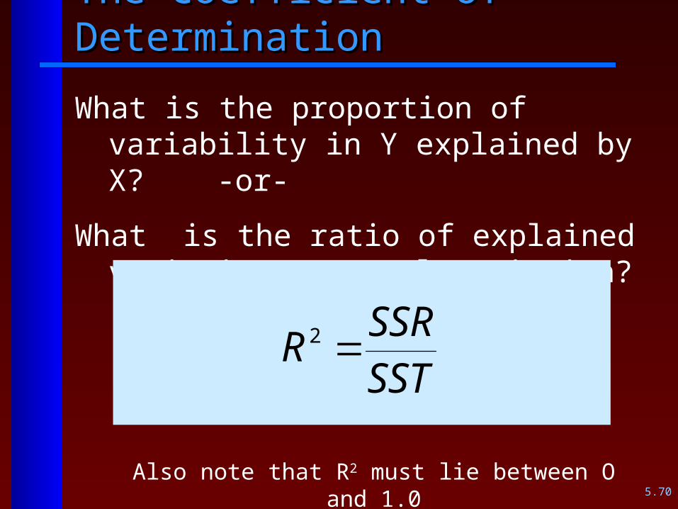
The Coefficient of DeterminationThe Coefficient of Determination

What is the proportion of variability in Y explained by X? -or-

What is the ratio of explained variation to total variation?

SSTSSR

R 2

Note: R2 = r2

5.70

The Coefficient of DeterminationThe Coefficient of Determination

What is the proportion of variability in Y explained by X? -or-

What is the ratio of explained variation to total variation?

SSTSSR

R 2

Also note that R2 must lie between O and 1.0

5.71

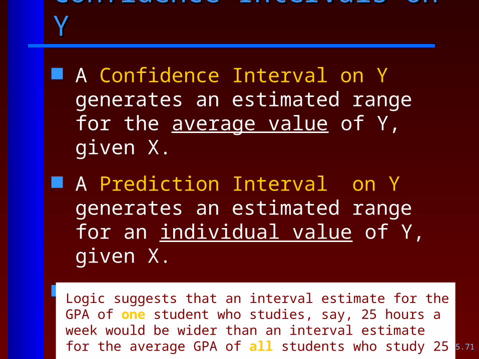
Confidence Intervals on YConfidence Intervals on Y

A Confidence Interval on Y generates an estimated range for the average value of Y, given X.

A Prediction Interval on Y generates an estimated range for an individual value of Y, given X.

Which of these intervals will be wider?

Logic suggests that an interval estimate for the GPA of one student who studies, say, 25 hours a week would be wider than an interval estimate for the average GPA of all students who study 25 hours a

week.

5.72

Confidence Intervals on YConfidence Intervals on Y

A Confidence Interval on Y generates an estimated range for the average value of Y, given X.

A Prediction Interval on Y generates an estimated range for an individual value of Y, given X.

Which of these intervals will be wider?

Prediction Intervals will be considerably wider than Confidence

Intervals on the same data.

5.73

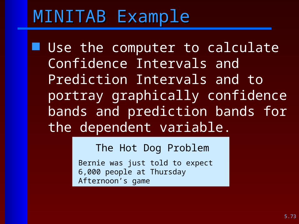
MINITAB ExampleMINITAB Example

Use the computer to calculate Confidence Intervals and Prediction Intervals and to portray graphically confidence bands and prediction bands for the dependent variable.

The Hot Dog ProblemBernie was just told to expect 6,000 people at Thursday Afternoon’s game

5.74

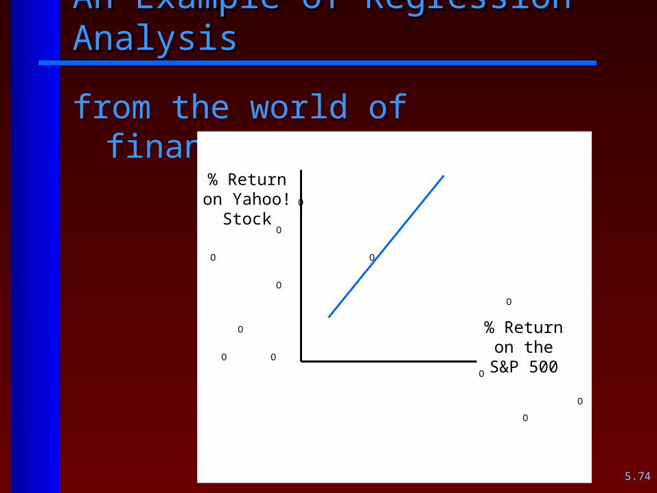
An Example of Regression AnalysisAn Example of Regression Analysis

from the world of finance . . .

O

O

O O

O

O

O

O O

O

O

O

% Return on the S&P

500

% Return on Yahoo! Stock

5.75



O

O

O O

O

O

O

O O

O

O

O

% Return on the S&P

500


bXaYX ˆ

5.76



O

O

O O

O

O

O

O O

O

O

O

% Return on the S&P

500


500 P&S%

Yahoo!%

return

returnb

5.77

A Stock’s “Beta”A Stock’s “Beta” Beta is the slope of the regression line

Betas greater than 1.0 describe a stock whose return is more variable than the return on the market as a whole (risky!).

Stocks with Betas of less than 1.0 are less volatile than the stock market as a whole

Examples of actual Betas:

Bed, Bath, and Beyond 1.02

Consolidated Edison .49

General Electric 1.17

Sun Microsystems 1.84

Merck Medco .70

5.78

Closing ThoughtsClosing Thoughts

Evaluate the statistical significance of a potential predictor variable on the basis of the t statistic and the associated P-Value.

Evaluate the strength of the regression model for any given problem on the basis of the Coefficient of Determination

How would you interpret problem results of a very low P-Value on the predictor variable AND a very low coefficient of determination?

Remember: If any of the three assumptions of least squares regression are violated, your regression model is not valid for making predictions.

5.79

In Preparation for Exam # 5In Preparation for Exam # 5

Do Study Questions (handout)

part v correlation analysis & simple regression dr. stephen h. russell weber state university

Documents

correlation analysis

correlation coefficient

n informal analysis

strength n

linear correlation

sample r slide

fsquare footage n

example regression equation