part vi regression with qualitative...
TRANSCRIPT

Regression with Qualitative Information
Part VI
Regression with Qualitative Information
As of Oct 15, 2019Seppo Pynnonen Econometrics I
Regression with Qualitative Information
1 Regression with Qualitative Information
Single Dummy Independent Variable
Multiple Categories
Ordinal Information
Interaction Involving Dummy Variables
Interaction among Dummy Variables
Different Slopes
Chow Test
Binary Dependent Variable
The Linear Probability Model
The Logit and Probit Model
Seppo Pynnonen Econometrics I

Regression with Qualitative Information
Qualitative information: ”family owns a car or not”, ”a personsmokes or not”, ”firm is in bankruptcy or not”, ”industry of afirm”, ”gender of a person”, etc
Some of the above examples can be both in a role of background(independent) variable or dependent variable.
Technically these kinds of variables are coded by a binary values (1= ”yes”) (0 = ”no”). In Econometrics these variables are calledgenerally called dummy variables.
Remark 6.1 Usual practice is to denote the dummy variable by the name
of one of the categories. For example, instead of using gender one can
define the variable e.g. as female, which equals 1 if the gender is female
and 0 if male.
Seppo Pynnonen Econometrics I

Regression with Qualitative Information
Exploring Further (W 5ed 7.1, p. 216)
Suppose, in a study comparing election outcomes between Democratic
and Republican candidates, the researcher wishes to indicate the party of
each candidate. Is a name such as party a wise choice for a binary
variable in this case. What would be a better name?
Seppo Pynnonen Econometrics I

Regression with Qualitative Information
Single Dummy Independent Variable
1 Regression with Qualitative Information
Single Dummy Independent Variable
Multiple Categories
Ordinal Information
Interaction Involving Dummy Variables
Interaction among Dummy Variables
Different Slopes
Chow Test
Binary Dependent Variable
The Linear Probability Model
The Logit and Probit Model
Seppo Pynnonen Econometrics I

Regression with Qualitative Information
Single Dummy Independent Variable
Dummy variables can be incorporated into a regression model asany other variables.
Consider the simple regression
y = β0 + δ0D + β1x + u, (1)
where D = 1 if individual has the property and D = 0 otherwise,and E[u|D, x ] = 0. Parameter δ0 indicated the difference withrespect to the reference group (D = 0), for which the parameter isβ0.
Thenδ0 = E[y |D = 1, x ]− E[y |D = 0, x ]. (2)
The value of x is same in both expectations, thus the difference isonly due to the property D.
Seppo Pynnonen Econometrics I

Regression with Qualitative Information
Single Dummy Independent Variable
-
6
��������
����
����
����
����
���
��������
����
����
����
����
���
x
y
E[y |D = 0, x ] = β0 + β1x
E[y |D = 1, x ] = β0 + δ0 + β1x
β0
β0 + δ0
Figure 6.1: E[y |D, x ] = β0 + δ0D + β1x + u, δ0 > 0.
The category with D = 0 makes the reference category, and δ0
indicates the change in the intercept with respect to the referencegroup.
Seppo Pynnonen Econometrics I

Regression with Qualitative Information
Single Dummy Independent Variable
From interpretation point of view it may also be beneficial toassociate the categories directly to the regression coefficients.
Consider the wage example, where
log(w) = β0 + β1educ + β2exper + β3tenure + u. (3)
Suppose we are interested about the difference in wage levelsbetween men an women. Then we can model β0 as a function ofgender as
β0 = βm + δffemale, (4)
where subscripts m and f refer to male and female, respectively.Model (3) can be written as
log(w) = βm + δffemale + β1educ
+β2exper + β3tenure + u.(5)
Seppo Pynnonen Econometrics I

Regression with Qualitative Information
Single Dummy Independent Variable
In the model the female dummy is zero for men. All other factorsremain the same. Thus the expected difference between wages interms of the model is according to (2) equal to δf
Because the left hand side is in logs, 100 δf indicates the differenceapproximately in percentages.
Seppo Pynnonen Econometrics I

Regression with Qualitative Information
Single Dummy Independent Variable
The log approximation may be inaccurate if the percentagedifference is big.
A more accurate approximation is obtained by using the fact that
log(wf )− log(wm) = log(wf /wm),
where wf and wm refer to a woman’s and a man’s wage,respectively, thus
100
(wf − wm
wm
)% = 100 (exp(δf)− 1) %. (6)
Seppo Pynnonen Econometrics I

Regression with Qualitative Information
Single Dummy Independent Variable
Example 1
Augment the wage example with squared exper and squared tenure toaccount for possible reducing incremental effect of experience and tenureand account for the possible wage difference with the female dummy.Thus the model is
log(w) = βm + δf female + β1educ
+β2exper + β3tenure
+β4(exper)2 + β5(tenure)2 + u.
(7)
Seppo Pynnonen Econometrics I

Regression with Qualitative Information
Single Dummy Independent Variable
Example 1 continues
Dependent Variable: LOG(WAGE)
Included observations: 526
=======================================================
Variable Coefficient Std. Error t-Statistic Prob.
-------------------------------------------------------
C 0.416691 0.098928 4.212066 0.0000
FEMALE -0.296511 0.035805 -8.281169 0.0000
EDUC 0.080197 0.006757 11.86823 0.0000
EXPER 0.029432 0.004975 5.915866 0.0000
TENURE 0.031714 0.006845 4.633036 0.0000
EXPER^2 -0.000583 0.000107 -5.430528 0.0000
TENURE^2 -0.000585 0.000235 -2.493365 0.0130
======================================================
R-squared 0.440769 Mean dependent var 1.623268
Adjusted R-squared 0.434304 S.D. dependent var 0.531538
S.E. of regression 0.399785 Akaike info criterion 1.017438
Sum squared resid 82.95065 Schwarz criterion 1.074200
F-statistic 68.17659 Prob(F-statistic) 0.000000
===========================================================
Seppo Pynnonen Econometrics I

Regression with Qualitative Information
Single Dummy Independent Variable
Example 1 continues
Using (6), with δf = −0.296511
100wf − wm
wm= 100[exp(δf)− 1] ≈ −25.7%, (8)
which suggests that, given the other factors, women’s wages (wf ) are onaverage 25.7 percent lower than men’s wages (wm).
It is notable that exper and tenure squared have statistically significant
negative coefficient estimates, which supports the idea of diminishing
marginal increase due to these factors.
Seppo Pynnonen Econometrics I

Regression with Qualitative Information
Multiple Categories
1 Regression with Qualitative Information
Single Dummy Independent Variable
Multiple Categories
Ordinal Information
Interaction Involving Dummy Variables
Interaction among Dummy Variables
Different Slopes
Chow Test
Binary Dependent Variable
The Linear Probability Model
The Logit and Probit Model
Seppo Pynnonen Econometrics I

Regression with Qualitative Information
Multiple Categories
Additional dummy variables can be included to the regressionmodel as well. In the wage example if married (married = 1, ifmarried, and 0, otherwise) is included we have the followingpossibilities
female married characteization
1 0 single woman1 1 married woman0 1 married man0 0 single man
and the intercept parameter refines to
β0 = βsm + δf female + δmamarr. (9)
Coefficient δma is the wage ”marriage premium”.
Seppo Pynnonen Econometrics I

Regression with Qualitative Information
Multiple Categories
Example 2
Including ”married” dummy into the wage model yields
Dependent Variable: LOG(WAGE)
Method: Least Squares
Sample: 1 526
Included observations: 526
======================================================
Variable Coefficient Std. Error t-Statistic Prob.
------------------------------------------------------
C 0.41778 0.09887 4.226 0.0000
FEMALE -0.29018 0.03611 -8.036 0.0000
MARRIED 0.05292 0.04076 1.299 0.1947
EDUC 0.07915 0.00680 11.640 0.0000
EXPER 0.02695 0.00533 5.061 0.0000
TENURE 0.03130 0.00685 4.570 0.0000
EXPER^2 -0.00054 0.00011 -4.813 0.0000
TENURE^2 -0.00057 0.00023 -2.448 0.0147
======================================================
R-squared 0.443 Mean dependent var 1.623
Adjusted R-squared 0.435 S.D. dependent var 0.532
S.E. of regression 0.400 Akaike info crit. 1.018
Sum squared resid 82.682 Schwarz criterion 1.083
Log likelihood -259.731 F-statistic 58.755
Durbin-Watson stat 1.798 Prob(F-statistic) 0.000
======================================================
Seppo Pynnonen Econometrics I

Regression with Qualitative Information
Multiple Categories
Example 2 continues
The estimate of the ”marriage premium” is about 5.3%, but it is notstatistically significant.
A major limitation of this model is that it assumes that the marriagepremium is the same for men and women.
We relax this next.
Seppo Pynnonen Econometrics I

Regression with Qualitative Information
Multiple Categories
Generating dummies: ”singfem”, ”marrfem”, and ”marrmale” wecan investigate the ”marriage premiums” for men and women.
The intercept term becomes
β0 = βsm + δmmmarrmale
+δmfmarrfem + δsfsingfem.(10)
The needed dummy-variables can be generated as cross-productsform the ”female” and ”married” dummies.
For example, the ”singfem” dummy is
singfem = (1−married)× female.
So, how do you generate ”marrmale” (married man)?
Seppo Pynnonen Econometrics I

Regression with Qualitative Information
Multiple Categories
Example 3
Estimating the model with the intercept modeled as (10) gives
Dependent Variable: LOG(WAGE)
Method: Least Squares
Sample: 1 526
Included observations: 526
======================================================
Variable Coefficient Std. Error t-Statistic Prob.
------------------------------------------------------
C 0.3214 0.1000 3.213 0.0014
MARRMALE 0.2127 0.0554 3.842 0.0001
MARRFEM -0.1983 0.0578 -3.428 0.0007
SINGFEM -0.1104 0.0557 -1.980 0.0483
EDUC 0.0789 0.0067 11.787 0.0000
EXPER 0.0268 0.0052 5.112 0.0000
TENURE 0.0291 0.0068 4.302 0.0000
EXPER^2 -0.0005 0.0001 -4.847 0.0000
TENURE^2 -0.0005 0.0002 -2.306 0.0215
======================================================
R-squared 0.461 Mean dependent var 1.623
Adjusted R-squared 0.453 S.D. dependent var 0.532
S.E. of regression 0.393 Akaike info crit. 0.988
Sum squared resid 79.968 Schwarz criterion 1.061
Log likelihood -250.955 F-statistic 55.246
Durbin-Watson stat 1.785 Prob(F-statistic) 0.000
======================================================
Seppo Pynnonen Econometrics I

Regression with Qualitative Information
Multiple Categories
Example 3 continues
The reference group is single men.
Single women and men estimated wage difference:-11.0%, just borderline statistically significant in the two sided test.
”Marriage premium” for men: 21.3% (more accurately, using (6), 23.7%).
Married women are estimated to earn 19.8% less than single men.
”Marriage premium” for women:
δmf − δsf ≈ −0.198− (−0.110) = −0.088
or −8.8%.
The statistical significance of this can be tested either directly or by
redefining the dummies such that the single women become the base.
Seppo Pynnonen Econometrics I

Regression with Qualitative Information
Multiple Categories
Example 3 continues
The direct testing can be worked out using advanced econometricsoftware (SAS, EViews, . . . ).
For example EViews Wald test produces for
H0 : δmf = δsf (11)
F = 2.821 (df 1 and 517) with p-value 0.0937, which is not statisticallysignificant and there is not empirical evidence for wage differencebetween married and single women.
In the same manner testing for H0 : δmm = δmf produces F = 80.61 withp-value 0.0000, i.e., highly statistically significant. Thus, there is strongempirical evidence of ’marriage premium’ for men.
Seppo Pynnonen Econometrics I

Regression with Qualitative Information
Multiple Categories
Remark 1
If there are q then q − 1 dummy variables are needed. The category
which does not have a dummy variable becomes the base category or
benchmark.
Remark 2
”Dummy variable trap”. If the model includes the intercept term,
defining q dummies for q categories leads to an exact linear dependence,
because 1 = D1 + · · ·+ Dq. Note also that D2 = D, which again leads
to an exact linear dependency if a ”dummy squared” is added to the
model. All these cases which lead to the exact linear dependency with
dummy-variables are called the ”dummy variable trap”.
Seppo Pynnonen Econometrics I

Regression with Qualitative Information
Multiple Categories
Exploring Further (W 5ed 7.2, p. 227)
In the baseball salary data MLB1 (available at www.econometrics.com),
players are given one of six positions: frstbase, scndbase, thrdbase,
shrtsop, outfield, or catcher. To allow for salary differentials accross
position, with outfielders as the base group, which dummy variables
would you include as independent variables?
Seppo Pynnonen Econometrics I

Regression with Qualitative Information
Multiple Categories
1 Regression with Qualitative Information
Single Dummy Independent Variable
Multiple Categories
Ordinal Information
Interaction Involving Dummy Variables
Interaction among Dummy Variables
Different Slopes
Chow Test
Binary Dependent Variable
The Linear Probability Model
The Logit and Probit Model
Seppo Pynnonen Econometrics I

Regression with Qualitative Information
Multiple Categories
If the categories include ordinal information (e.g. 1 = ”good”, 2 =”better”, 3 = ”best”), sometimes people these variables as such inregressions. However, interpretation may be a problem, because”one unit change” implies a constant partial effect. That is thedifference between ”better” and ”good” is as big as ”best” and”better”.
Seppo Pynnonen Econometrics I

Regression with Qualitative Information
Multiple Categories
The usual alternative to use dummy-variables. In the aboveexample two dummies are needed. D1 = 1 is ”better”, and 0otherwise, D2 = 1 for ”best” and 0 otherwise. As a consequence,the reference group is ”good”.
Seppo Pynnonen Econometrics I

Regression with Qualitative Information
Multiple Categories
Exploring Further (Adapted from W 5ed 7.3, p228)
Consider the effect of credit rating (CR) on the municipal bond rate(MBR). Credit ratings are indicated by ranking from zero to four, withzero the worst and four being the best. Using using model
MBR = β0 + δ1 CR1 + δ2 CR2 + δ3 CR3 + δ4 CR4 + other factors,
where CR1 = 1 if CR = 1, and CR1 = 0 otherwise, CR2 = 1 if CR = 2,and CR2 = 0 otherwise, and so on.
What can you expect about the signs of the coefficients δi?
How would you test that credit rating has no effect on MBR?
Seppo Pynnonen Econometrics I

Regression with Qualitative Information
Multiple Categories
The constant partial effect can be tested by testing the restrictedmodel
y = β0 + δ(D1 + 2D2) + β1x + u (12)
against the unrestricted alternative
yi = β0 + δ1D1 + δ2D2 + β1x + u. (13)
Exploring Further
How would you test using Eviews whether the credit rating affects
linearly on the municipal bond rate?
Seppo Pynnonen Econometrics I

Regression with Qualitative Information
Multiple Categories
Example 4
Effects of law school ranking on starting salaries. Dummy variablestop10, r11 25, r26 40, r41 60, and r61 100. The reference group is theschools ranked below 100.
Seppo Pynnonen Econometrics I

Regression with Qualitative Information
Multiple Categories
Example 4 continues
Below are estimation results with some additional covariates
(Wooldridge, Example 7.8).
Dependent Variable: LOG(SALARY)
Sample (adjusted): 1 155
Included observations: 136 after adjustments
======================================================
Variable Coefficient Std. Error t-Statistic Prob.
------------------------------------------------------
C 9.1653 0.4114 22.277 0.0000
TOP10 0.6996 0.0535 13.078 0.0000
R11_25 0.5935 0.0394 15.049 0.0000
R26_40 0.3751 0.0341 11.005 0.0000
R41_60 0.2628 0.0280 9.399 0.0000
R61_100 0.1316 0.0210 6.254 0.0000
LSAT 0.0057 0.0031 1.858 0.0655
GPA 0.0137 0.0742 0.185 0.8535
LOG(LIBVOL) 0.0364 0.0260 1.398 0.1647
LOG(COST) 0.0008 0.0251 0.033 0.9734
======================================================
R-squared 0.911 Mean dependent var 10.541
Adjusted R-squared 0.905 S.D. dependent var 0.277
S.E. of regression 0.086 Akaike info crit. -2.007
Sum squared resid 0.924 Schwarz criterion -1.792
F-statistic 143.199 Prob(F-statistic) 0.000
======================================================
Seppo Pynnonen Econometrics I

Regression with Qualitative Information
Multiple Categories
Example 4 continues
The estimation results indicate that the ranking has a big influence onthe staring salary.
The estimated median salary at a law school ranked between 61 and 100is about 13% higher than in those ranked below 100.
The coefficient estimate for the top 10 is 0.6996, using (6) we get
100 [exp(0.6996)− 1] ≈ 101.4%, that is median starting salaries in top
10 schools tend to be double to those ranked below 100.
Seppo Pynnonen Econometrics I

Regression with Qualitative Information
Multiple Categories
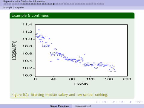
Example 5
Although not fully relevant, let us for just illustration purposes testconstant partial effect hypothesis. I.e., whether
H0 :
δtop10 = 5δ61 100,δ11 25 = 4δ61 100,δ26 40 = 3δ61 100,δ41 60 = 2δ61 100.
(14)
Using Wald test for coefficient restrictions in EViews gives F = 1.456with df1 = 4 and df2 = 126 and p-value 0.2196.
This indicates that the there is not much empirical evidence against the
constant partial effect for the starting salary increment. The estimated
constant partial coefficient is 0.139782, i.e., at each ranking class starting
median salary is estimated to increase approximately by 14%.
Seppo Pynnonen Econometrics I
Regression with Qualitative Information
Multiple Categories
Example 5 continues
10.0
10.2
10.4
10.6
10.8
11.0
11.2
11.4
0 40 80 120 160 200
RANK
LOG(
SALA
RY)
Figure 6.1: Starting median salary and law school ranking.
Seppo Pynnonen Econometrics I

Regression with Qualitative Information
Interaction Involving Dummy Variables
1 Regression with Qualitative Information
Single Dummy Independent Variable
Multiple Categories
Ordinal Information
Interaction Involving Dummy Variables
Interaction among Dummy Variables
Different Slopes
Chow Test
Binary Dependent Variable
The Linear Probability Model
The Logit and Probit Model
Seppo Pynnonen Econometrics I

Regression with Qualitative Information
Interaction Involving Dummy Variables
In Example 3 additional dummy variables were generated bymultiplying various other dummy variables.
Factually these define interaction terms among dummy variables.
Example 6
The same model as in Example 3 can be specified as
log(wage) = β0+δf female+δmarmarried+δm×f (female×married)+· · ·(15)
Seppo Pynnonen Econometrics I

Regression with Qualitative Information
Interaction Involving Dummy Variables
Example 6 continueslm(formula = log(wage) ~ female + married + I(female * married) +
educ + educ + exper + tenure + I(exper^2) + I(tenure^2),
data = wdfr)
Residuals:
Min 1Q Median 3Q Max
-1.89697 -0.24060 -0.02689 0.23144 1.09197
Coefficients:
Estimate Std. Error t value Pr(>|t|)
(Intercept) 0.3213781 0.1000090 3.213 0.001393 **
female -0.1103502 0.0557421 -1.980 0.048272 *
married 0.2126757 0.0553572 3.842 0.000137 ***
I(female * married) -0.3005931 0.0717669 -4.188 3.30e-05 ***
educ 0.0789103 0.0066945 11.787 < 2e-16 ***
exper 0.0268006 0.0052428 5.112 4.50e-07 ***
tenure 0.0290875 0.0067620 4.302 2.03e-05 ***
I(exper^2) -0.0005352 0.0001104 -4.847 1.66e-06 ***
I(tenure^2) -0.0005331 0.0002312 -2.306 0.021531 *
---
Signif. codes: 0 *** 0.001 ** 0.01 * 0.05 . 0.1 1
Residual standard error: 0.3933 on 517 degrees of freedom
Multiple R-squared: 0.4609,Adjusted R-squared: 0.4525
F-statistic: 55.25 on 8 and 517 DF, p-value: < 2.2e-16
Seppo Pynnonen Econometrics I

Regression with Qualitative Information
Interaction Involving Dummy Variables
Example 6 continues
This example allows to estimate wage differential for all the four groups(single men, single women, married men, married women), but we needto be careful in deriving the differentials.
It is better to compute the differential as differences of the intercepts ofthe groups.
For example marriage premium for women (compared to single women):The intercept for married women is β0 + δf + δmar + δm×f and theintercept for single women is β0 + δf , such that the difference isδmar + δm×f with estimate 0.2126757− 0.3005931 ≈ 0.088 as inExample 3.
We observe that the marriage premium for men to single men in this
specification is directly δmar (= β0 + δmar − β0).
Seppo Pynnonen Econometrics I

Regression with Qualitative Information
Interaction Involving Dummy Variables
1 Regression with Qualitative Information
Single Dummy Independent Variable
Multiple Categories
Ordinal Information
Interaction Involving Dummy Variables
Interaction among Dummy Variables
Different Slopes
Chow Test
Binary Dependent Variable
The Linear Probability Model
The Logit and Probit Model
Seppo Pynnonen Econometrics I

Regression with Qualitative Information
Interaction Involving Dummy Variables
Considery = β0 + β1x1 + u. (16)
If the slope depends also on the group, we get in addition to
β0 = β00 + δ0D, (17)
for the slope coefficient similarly
β1 = β11 + δ1D. (18)
The regression equation is then
y = β00 + δ0D + β11x1 + δ1x2 + u, (19)
where x2 = D x1.
Seppo Pynnonen Econometrics I

Regression with Qualitative Information
Interaction Involving Dummy Variables
Example 7
Wage example. Test whether return to eduction differs between womenand men. This can be tested by defining
βeduc = βmeduc + δfeducfemale. (20)
The null hypothesis is H0 : δfeduc = 0.
Seppo Pynnonen Econometrics I

Regression with Qualitative Information
Interaction Involving Dummy Variables
Example 7 continuesDependent Variable: LOG(WAGE)
Method: Least Squares
Sample: 1 526
Included observations: 526
======================================================
Variable Coefficient Std. Error t-Statistic Prob.
------------------------------------------------------
C 0.31066 0.11831 2.626 0.0089
MARRMALE 0.21228 0.05546 3.828 0.0001
MARRFEM -0.17093 0.17100 -1.000 0.3180
SINGFEM -0.08340 0.16815 -0.496 0.6201
FEMALE*EDUC -0.00219 0.01288 -0.170 0.8652
EDUC 0.07976 0.00838 9.521 0.0000
EXPER 0.02676 0.00525 5.095 0.0000
TENURE 0.02916 0.00678 4.299 0.0000
EXPER^2 -0.00053 0.00011 -4.829 0.0000
TENURE^2 -0.00054 0.00023 -2.309 0.0213
======================================================
R-squared 0.461 Mean dependent var 1.623
Adjusted R-squared 0.452 S.D. dependent var 0.532
S.E. of regression 0.394 Akaike info crit. 0.992
Sum squared resid 79.964 Schwarz criterion 1.073
Log likelihood -250.940 F-statistic 49.018
Durbin-Watson stat 1.785 Prob(F-statistic) 0.000
======================================================
Seppo Pynnonen Econometrics I

Regression with Qualitative Information
Interaction Involving Dummy Variables
Example 7 continues
δfeduc = −0.00219 with p-value 0.8652.
Thus there is no empirical evidence that return to education would differbetween men and women.
Below are wage graphs for men and women as functions of education
evaluated at the mean of the other variables.
Seppo Pynnonen Econometrics I

Regression with Qualitative Information
Interaction Involving Dummy Variables
Example 7 continues
● ●●
●●
●
●
●
●
●
●
●●
●
●
●
●
●
●
●
●●
●
●
●
●●
●●
●
●
●
●
●●●
●
●●
●
●
●
●●
●
●
●
●
●
●
●
●
●●
●
● ●
●
●
●
● ●
●
●
●
●
●
●
●
●
●
●
●
●
●
●
●
●
●●
● ●
●
●
●●●
●●
●
●
●
●
●
●
●●
●
●●
●
●●
●
●
●
●
●
●
●
●
●
●●
●● ●● ●
●
●●
●●●
●●
●
●
●
●
●
●●
●
●
●
●
●
●●
●
●
●
●●
●
●
●
●●
●
●●
●
●
●
●
●
●
●●
●
●
●
●
●
●●
● ●●
●
●
●●
●●
●
●
●
●●
●●
●
●
●
●●
●
●
●
●
●
●●
●●
●
●
●●
●●
●
●
●
●
● ●●●
● ●
●
●
●●
●
● ●●
●
●
●
●
●
●
● ●
●
●●
●
●●●
●
●●●
●
●
●
●●
●
●
●
●
●●
●●
●
●
●
●
●
●
●●●
●
●
●
●
●
●
●
●
●
●
●
●
●
●
● ●
●
●
●●
●●
●
●
●
●●
●
●●
●
●
●●
●
●
●
●
●
●
●●
●
●● ●
●
●
●●
●●●
●
● ● ●
●●
●
●
●
●●●
●●
●
●
●
●●
●●
●
●
● ●
●
●
●
●●
●
●
●●
●
●
●
●
●
●
●●
●●
●
●
●●
●
● ●●
●
●
●
●
●
●
●
●
●
●●
●
●
●
●
●
●
●
●●
●
●
●
●
●
●
●●
●
●
●
●●●
●
●●
●
●●●
●●
●
●
●●
●
●
●
●●
●
●
●● ●
●
●●
●
●
●
●
●
●●
●
●
●
●
●
●
●
●
●
●●
●
●
●
●●
●
●
●
●●
●
●
●
●●
●●
●
●
●
●
●
●
●●
●●
●
●
●●
●
●
●●●
●
●
●
●
●
●
●
●
●
●
●
●●
●
●
●
●
●
●
● ●
●
●
●
●
●
●
●
●
●
●
●
●
●
●
●
●●
●
●
●
●
●
0 5 10 15
01
23
Wages and EducationPanel A: Logarithmic scale
Education (years)
Hou
rly w
age
(log)
MenWomen
● ●●
●●
●
●
●
●
●
●
●●
●
●
●
●
●
●●
●
●
●
●
●
●
●
●●
●
●
●
●
●● ●
●
● ●
●
●
●
●●
●
●
●●
●●●
●
●●
●● ●
●
●
●
●●
●
●
●
●
●
●
●
●
●
●
●
●●
●
●●
●●
● ●
●
●
●●●
●
●
●
●
●
●
●
●
● ●
●
●●
●
●●
●
●
●
●
●
●
●
●
●
●●
●● ●● ●●
●●
●●●
●●
●
●
●
●
●
●●
●
●
●
●
●
●●
●
●●
●●
●
●
●
●●
●
●●
●
●
●
●
●
●
●●
●
●
●
●
●
●●
●●
●
●
●
●●
●●
●
●
●
●●
●●
●
●
●●●●
●
●
●
●
●●
●●
●
●
●●
●●
●
●
●
●
● ● ●●
● ●
●
●
●●
●
● ●●●
●
●
●
●
●
●●
●
●●
●
● ●●●●●●
●
●
●
●●
●
●●
●●
●●●
●
●●
●
●
●●●●
●
●
●
●●
●
●
●
●
●
●
●
●
●
● ●
●
●
●●
●●
●
●
●
●●
●
●●●
●
●●
●
●
●
●
●●
●●
●
●● ●
●
●
●●
●●●
●● ● ●
●●
●
●
●
●●●
● ●
●
●
●
●●
●●
●
●
● ●
●
●●
●●
●
●
●●
●
●●
●
●
●
●●
●●
●●●●
●● ●●●
●
●
●
●
●
●
●
●
● ●
●
●
●
●
●
●
●● ●
●
●●
●
●
●
●●
●
●
●
●●●
●
●●
●
●●●
●●
●
●
●●
●
●●
●●
●
●
●● ●
●
● ●
●
●
●
●
●
●●
●
●●
●
●
●
●
●
●
●●
●
●
●
●●
●
●
●
● ●
●
●
●
●●● ●
●
●●
●
●
●
● ●
●●
●
●
●●
●
●●●
●
●
●
●
●
●
●
●
●
●●
●●●
●
●
●
●
●●
● ●
●
●
●
●
●
●
●
●
●
●
●
●
●
●
●
●●
●
●
●
●
●
0 5 10 15
05
1015
2025
Panel B: Original scale
Education (years)
Hou
rly w
age
(USD
/hou
r)
MenWomen
Seppo Pynnonen Econometrics I

Regression with Qualitative Information
Interaction Involving Dummy Variables
Exploring further
Can you explain the incremental regression line differentials between
women and men in Panel B of the above figure?
Exploring further 7.4 W 5ed, p.234
How would you augment model in Example 7 to allow the return to
tenure to differ by gender?
Seppo Pynnonen Econometrics I

Regression with Qualitative Information
Interaction Involving Dummy Variables
1 Regression with Qualitative Information
Single Dummy Independent Variable
Multiple Categories
Ordinal Information
Interaction Involving Dummy Variables
Interaction among Dummy Variables
Different Slopes
Chow Test
Binary Dependent Variable
The Linear Probability Model
The Logit and Probit Model
Seppo Pynnonen Econometrics I

Regression with Qualitative Information
Interaction Involving Dummy Variables
Suppose there are two populations (e.g. men and women) and wewant to test whether the same regression function applies to bothgroups.
All this can be handled by introducing a dummy variable, D withD = 1 for group 1 and zero for group 2.
Seppo Pynnonen Econometrics I

Regression with Qualitative Information
Interaction Involving Dummy Variables
If the regression in group g (g = 1, 2) is
yg ,i = βg ,0 + βg ,1xg ,i,1 + · · ·+ βg ,kxg ,i,k + ug ,i , (21)
i = 1, . . . , ng , where ng is the number of observations from groupg .
Using the group dummy, we can write
βg ,j = βj + δjD, (22)
j = 0, 1, . . . , k . An important assumption is that in both groupsvar[ug ,i ] = σ2
u.
The null hypothesis is
H0 : δ0 = δ1 = · · · = δk = 0. (23)
Seppo Pynnonen Econometrics I

Regression with Qualitative Information
Interaction Involving Dummy Variables
The null hypothesis (23) can be tested with the F -test, given in(4.20).
In the first step the unrestricted model is estimated over thepooled sample with coefficients of the form in equation (21) (thus2(k + 1)-coefficients).
Next the restricted model, with all δ-coefficients set to zero, isestimated again over the pooled sample.
Using the SSRs from restricted and unrestricted models, teststatistic (4.20) becomes
F =(SSRr − SSRur )/(k + 1)
SSRur/[n − 2(k + 1)], (24)
which has the F -distribution under the null hypothesis with k + 1and n − 2(k + 1) degrees of freedom.
Seppo Pynnonen Econometrics I

Regression with Qualitative Information
Interaction Involving Dummy Variables
Exactly the same result is obtained if one estimates the regressionequations separately from each group and sums up the SSRs. Thatis
SSRur = SSR1 + SSR2, (25)
Where SSRg is from the regression estimated from group g ,g = 1, 2.
Thus, statistic (24) can be written alternatively as
F =[SSRr − (SSR1 + SSR2)]/(k + 1)
(SSR1 + SSR2)/[n − 2(k + 1)], (26)
which is known as Chow statistic (or Chow test).
Seppo Pynnonen Econometrics I
Regression with Qualitative Information
Binary Dependent Variable
1 Regression with Qualitative Information
Single Dummy Independent Variable
Multiple Categories
Ordinal Information
Interaction Involving Dummy Variables
Interaction among Dummy Variables
Different Slopes
Chow Test
Binary Dependent Variable
The Linear Probability Model
The Logit and Probit Model
Seppo Pynnonen Econometrics I

Regression with Qualitative Information
Binary Dependent Variable
Up until now in regression
y = x′β + u, (27)
where x′β = β0 + β1x1 + · · ·+ βkxk , y has had quantitativemeaning (e.g. wage).
What if y indicates a qualitative event (e.g., firm has gone tobankruptcy), such that y = 1 indicates the occurrence of theevent (”success”) and y = 0 non-occurrence (”fail”), and wewant to explain it by some explanatory variables?
Seppo Pynnonen Econometrics I

Regression with Qualitative Information
Binary Dependent Variable
The meaning of the regression
y = x′β + u,
when y is a binary variable. Then, because E[u|x] = 0,
E[y |x] = x′β. (28)
Because y is a random variable that can have only values 0 or 1,we can define probabilities for y as P(y = 1|x) andP(y = 0|x) = 1− P(y = 1|x), such that
E[y |x] = 0 · P(y = 0|x) + 1 · P(y = 1|x) = P(y = 1|x).
Seppo Pynnonen Econometrics I

Regression with Qualitative Information
Binary Dependent Variable
Thus, E[y |x] = P(y = 1|x) indicates the success probability andregression in equation 28 models
P(y = 1|x) = β0 + β1x1 + · · ·+ βkxk , (29)
the probability of success. This is called the linear probabilitymodel (LPM).
The slope coefficients indicate the marginal effect of correspondingx-variable on the success probability, i.e., change in the probabilityas x changes, or
∆P(y = 1|x) = βj∆xj . (30)
Seppo Pynnonen Econometrics I

Regression with Qualitative Information
Binary Dependent Variable
In the OLS estimated model
y = β0 + β1x1 + . . . βkxk (31)
y is the estimated or predicted probability of success.
In order to correctly specify the binary variable, it may be useful toname the variable according to the ”success” category (e.g., in abankruptcy study, bankrupt = 1 for bankrupt firms andbankrupt = 0 for non-bankrupt firm [thus ”success” is just ageneric term]).
Seppo Pynnonen Econometrics I

Regression with Qualitative Information
Binary Dependent Variable
Example 8
Married women participation in labor force (year 1975). (See R-snippetfor the R-commands)
Call:
lm(formula = inlf ~ huswage + educ + exper + I(exper^2) + age +
kidslt6 + kidsge6, data = mdfr)
Residuals:
Min 1Q Median 3Q Max
-0.95304 -0.37143 0.08112 0.33820 0.92459
Coefficients:
Estimate Std. Error t value Pr(>|t|)
(Intercept) 0.6067070 0.1536916 3.948 8.64e-05 ***
huswage -0.0081511 0.0039107 -2.084 0.0375 *
educ 0.0370734 0.0073371 5.053 5.48e-07 ***
exper 0.0404174 0.0056619 7.138 2.24e-12 ***
I(exper^2) -0.0006120 0.0001852 -3.304 0.0010 **
age -0.0165940 0.0024592 -6.748 3.02e-11 ***
kidslt6 -0.2636923 0.0335068 -7.870 1.25e-14 ***
kidsge6 0.0110821 0.0131915 0.840 0.4011
---
Signif. codes: 0 *** 0.001 ** 0.01 * 0.05 . 0.1 1
Residual standard error: 0.4275 on 745 degrees of freedom
Multiple R-squared: 0.2631,Adjusted R-squared: 0.2561
F-statistic: 37.99 on 7 and 745 DF, p-value: < 2.2e-16
Seppo Pynnonen Econometrics I

Regression with Qualitative Information
Binary Dependent Variable
Example 8 continues
All but kidsge6 are statistically significant with signs as might beexpected.
The coefficients indicate the marginal effects of the variables on theprobability that inlf = 1. Thus e.g., an additional year of educincreases the probability by 0.037 (other variables held fixed).
0 10 20 30 40
0.30.4
0.50.6
0.70.8
0.9
Marginal effect of experince on married women labor force participation
Experience (years)
Probab
ility
0 5 10 15
0.20.3
0.40.5
0.60.7
0.8
Marginal effect of eduction on married women labor force participation
Education (years)
Probab
ility
Seppo Pynnonen Econometrics I

Regression with Qualitative Information
Binary Dependent Variable
Some issues with associated to the LPM.
Dependent left hand side restricted to (0, 1), while right handside (−∞,∞), which may result to probability predictions lessthan zero or larger than one.
Heteroskedasticity of u, since by denotingp(x) = P(y = 1|x) = x′β
var[u|x ] = (1− p(x))p(x) (32)
which is not a constant but depends on x, and hence violatingAssumption 2.
Seppo Pynnonen Econometrics I

Regression with Qualitative Information
Binary Dependent Variable
1 Regression with Qualitative Information
Single Dummy Independent Variable
Multiple Categories
Ordinal Information
Interaction Involving Dummy Variables
Interaction among Dummy Variables
Different Slopes
Chow Test
Binary Dependent Variable
The Linear Probability Model
The Logit and Probit Model
Seppo Pynnonen Econometrics I

Regression with Qualitative Information
Binary Dependent Variable
The first of the above problems can be technically easily solved bymapping the linear function on the right hand side of equation 29by a non-linear function to the range (0, 1). Such a function isgenerally called a link function.
That is, instead we write equation (19) as
P(y = 1|x) = G (x′β). (33)
Although any function G : R→ [0, 1] applies in principle, so calledlogit and probit transformations are in practice most popular (theformer is based on logistic distribution and the latter normaldistribution).
Economists favor often the probit transformation such that G isthe distribution function of the standard normal density, i.e.,
G (z) = Φ(z) =
∫ z
−∞
1√2π
e−12v2dv , (34)
Seppo Pynnonen Econometrics I

Regression with Qualitative Information
Binary Dependent Variable
In the logit tranformation
G (z) =ez
1 + ez=
1
1 + e−z=
∫ z
−∞
e−v
(1 + e−v )2dv . (35)
Both as S-shaped
−3 −1 0 1 2 3
0.00.2
0.40.6
0.81.0
Probit transformation
z
G(z)
−3 −1 0 1 2 3
0.00.2
0.40.6
0.81.0
Logit transformation
z
G(z)
Seppo Pynnonen Econometrics I

Regression with Qualitative Information
Binary Dependent Variable
The price, however, is that the interpretation of the marginaleffects is not any more as straightforward as with the LPM.
However, negative sign indicates decreasing effect on theprobability and positive increasing.
Seppo Pynnonen Econometrics I

Regression with Qualitative Information
Binary Dependent Variable
Example 9
Probit and logit estimatation married women labor force participationprobability.Probit: (family = binomial(link = ”probit”) in glm)
glm(formula = inlf ~ huswage + educ + exper + I(exper^2) + age +
kidslt6 + kidsge6, family = binomial(link = "probit"), data = wkng)
Deviance Residuals:
Min 1Q Median 3Q Max
-2.2495 -0.9127 0.4288 0.8502 2.2237
Coefficients:
Estimate Std. Error z value Pr(>|z|)
(Intercept) 0.3606454 0.5045248 0.715 0.47472
huswage -0.0255438 0.0126530 -2.019 0.04351 *
educ 0.1248347 0.0249191 5.010 5.45e-07 ***
exper 0.1260736 0.0187091 6.739 1.60e-11 ***
I(exper^2) -0.0019245 0.0005987 -3.214 0.00131 **
age -0.0547298 0.0083918 -6.522 6.95e-11 ***
kidslt6 -0.8650224 0.1177382 -7.347 2.03e-13 ***
kidsge6 0.0285102 0.0438420 0.650 0.51550
---
Signif. codes: 0 *** 0.001 ** 0.01 * 0.05 . 0.1 1
Null deviance: 1029.75 on 752 degrees of freedom
Residual deviance: 804.69 on 745 degrees of freedom
AIC: 820.69
Seppo Pynnonen Econometrics I

Regression with Qualitative Information
Binary Dependent Variable
Example 9 continues
Logit: (family = binomial(link = ”logit”) in glm)
glm(formula = inlf ~ huswage + educ + exper + I(exper^2) + age +
kidslt6 + kidsge6, family = binomial(link = "logit"), data = wkng)
Deviance Residuals:
Min 1Q Median 3Q Max
-2.2086 -0.8990 0.4481 0.8447 2.1953
Coefficients:
Estimate Std. Error z value Pr(>|z|)
(Intercept) 0.592500 0.853042 0.695 0.48732
huswage -0.043803 0.021312 -2.055 0.03985 *
educ 0.209272 0.042568 4.916 8.83e-07 ***
exper 0.209668 0.031963 6.560 5.39e-11 ***
I(exper^2) -0.003181 0.001013 -3.141 0.00168 **
age -0.091342 0.014460 -6.317 2.67e-10 ***
kidslt6 -1.431959 0.202233 -7.081 1.43e-12 ***
kidsge6 0.047089 0.074284 0.634 0.52614
---
Signif. codes: 0 *** 0.001 ** 0.01 * 0.05 . 0.1 1
Null deviance: 1029.75 on 752 degrees of freedom
Residual deviance: 805.85 on 745 degrees of freedom
AIC: 821.85
Qualitatively the results are similar to those of the LPM. (R exercise: create similar
graphs to those of the linear case for the marginal effects.)
Seppo Pynnonen Econometrics I