participation in higher education : a geodemographic
TRANSCRIPT

38th Congress of the European Regional Science Association28 August - 1 September 1998, Vienna
PARTICIPATION IN HIGHER EDUCATION :A GEODEMOGRAPHIC PERSPECTIVE ON
THE POTENTIAL FOR FURTHER EXPANSIONIN STUDENT NUMBERS
Peter Batey and Peter Brown
Department of Civic Design, University of LiverpoolAbercromby Square, Liverpool L69 3BX, UK
e-mail addresses:[email protected] and [email protected]
Abstract
Higher education in England has expanded rapidly in the last ten years with the resultthat currently more than 30 per cent of young people go on to university. Expansion islikely to continue following the recommendations of a national committee of inquiry (theDearing Committee). The participation rate is known to vary substantially among socialgroups and between geographical areas. In this paper participation rate is calculatedusing a new measure, the Young Entrants Index (YEI), and establishes the extent ofvariation by region, gender and residential neighbourhood type. The Super Profilesgeodemographic system is used to facilitate the latter. This is shown to be a powerfuldiscriminator and to offer great potential as an alternative analytical approach to theconventional social class categories, based on parental occupation, that have formed thebasis of most participation studies to date.

2
1. INTRODUCTIONIn the last ten years or so, British higher education has undergone a major transformation
in terms of student numbers. Historically, the university system has catered for only a
small minority of young people and, as recently as 1989, just 16 per cent of school
leavers went on to university (Robertson and Hillman, 1997). A change in government
policy in the late 1980s led to a dramatic expansion in the university system with the
result that by 1993 the national participation rate among young entrants (age participation
index : API) had risen to more than 30 per cent. This expansion occurred much more
rapidly than the government had intended with the result that a cap was placed on any
further growth in publicly-funded full-time undergraduate student numbers. Among
OECD countries, Britain’s enrolment rates in universities are now among the highest,
exceeded only by those of Canada and the United States (The Economist, 1997).
Expansion in higher education is now firmly back on the political agenda in the UK.
The Terms of Reference of a National Committee of Inquiry into Higher Education
(the Dearing Committee), set up in 1996, included a specific statement that:
“there should be maximum participation in initial higher education by young and
mature students and in lifetime learning by adults, having regard to the needs of
individuals, the nation and the future labour market” (National Committee of
Inquiry into Higher Education, Summary Report, 1997 p.5).
The Dearing Committee’s final report concluded that higher education should resume its
growth:
“The UK must plan to match the participation rates of other advanced nations :
not to do so would weaken the basis of national competitiveness.” (National
Committee of Inquiry into Higher Education, Summary Report, 1997 p.13-14).
The report did not set a target figure for future participation, suggesting that student and
employer demand should be the main determinant of future growth. It did,
however, make comparisons within the UK and drew attention to the relatively high
participation rates in Scotland and Northern Ireland; in these countries as many as 45 per
cent of young people enter university. The Dearing Committee indicated that it would

3
not be unrealistic to expect the national (UK) participation to rise to this level within the
next twenty years.
This paper presents the results of an exploratory study designed to examine detailed
socio-economic and regional differentials in participation. It has long been recognised
that the characteristics of young entrants to higher education do not match those of the
population as a whole. This is particularly true of social groups, but the problems of
obtaining reliable data for students and the eligible population have hampered research in
this area, making it difficult to draw firm conclusions.
The present study was commissioned by the Higher Education Funding Council for
England (HEFCE). It employs a geodemographic system, Super Profiles, to analyse
these differentials, assigning a geodemographic category to each postcoded student
address.
A new participation index, the Young Entrant Index (YEI), closely related to the API,
is constructed. The dataset assembled for the research covers the home address of all
eligible students in England and Wales as well as an estimate of the 18 and 19 year old
age cohorts. The former serves as the numerator in constructing the YEI, while the mean
of the latter is used as the denominator.
The paper is organised into four main sections. In the next section a brief review is given
of earlier studies examining variations in participation rates, principally in terms of
variations by social groups. This approach has well-known drawbacks and this leads us
to propose an alternative method of analysis based on geodemographics. Section 3
outlines the methodology of the study, defining the measures of participation to be
employed, the geodemographic classifiers and the sources of data about students. In
Section 4 the results of the study are presented, by region, gender and geodemographic
group. An attempt is made to establish the relative contribution of geodemographic and
non-geodemographic factors to regional variations in the YEI. In a final section
conclusions are drawn and proposals are made for extending the present study to include
the analysis of change in participation rates over time.

4
2. VARIATIONS IN PARTICIPATION RATES
2.1 Analysis by Social Group
The assignment of individuals and groups to social classes and socio-economic groups is
based on an assessment of occupation (OPCS, 1990; 1991). Two such classifications are
widely used in Great Britain: Social Class (SC) based on Occupation and Socio-
Economic Groups (SEGs). A consistent finding of work on higher education
participation by social group is that SC I and II (professional and non-manual groups, are
equivalent) are over-represented at the expense of SC III to V (mainly manual groups, or
equivalent) sometimes to a significant degree. Egerton and Halsey (1993) took three
cohorts (born 1936-1945, 1946-1995 and 1956-1965), constructed from General
Household Survey data, to form a sample of 25,000 divided into Goldthorpe-Hope (GH)
classes I, II and III (broadly, I is socially privileged). They showed that exposure to
higher education rose from 17 per cent to 28 per cent of the cohort from the first to last
cohort for GH I, whereas for GH III the rise was from 2 per cent to 5 per cent. Noting
that previous work had shown no reduction in differences in participation between social
groups in this century, the researchers conclude that social groups inequalities will be
perpetuated.
Burnhill et al (1990) used a comprehensive survey of Scottish school leavers to examine
the effects of social class on participation. The probability of attaining the minimum
qualifications for higher education entrance was fitted to a model, and found to be largely
a function of social class and level of parental education. However, the progression from
minimum entrance qualifications to entering higher education was found to be much less
dependent on social class.
A social group bias was acknowledged in past projections of higher education students.
In 1984 the Royal Statistical Society’s Working Party on the Projections of Student
Numbers in Higher Education considered several projection models (Royal Statistical
Society, 1985). All included social group either explicitly or implicitly. The Working
Party recommended that calculations should take account of social group in projecting
participation. The Department of Education and Science (1986) published projections of
higher education students in 1986. The methodology employed modelled the Social
Class composition of the 18 year old population so that different attainment rates (for

5
minimum higher education entrance qualifications) could be applied for each class.
These assumed a range of attainment spanning from 50 per cent of OC80 1 (professional
and managerial) to under 5 per cent for OC80 V (unskilled).
2.2 Justification for a Geodemographic Approach
The assignment of individuals to social groups on the basis of their occupational
background has the advantage of treating people at an individual or household level and
allows ready comparison with other sources of data.
However, occupation-based systems suffer from a number of drawbacks:
a. Individuals are not completely characterised by their occupations, so a particular
social group may represent people with widely differing circumstances.
b. Collecting sufficiently detailed occupational information is time consuming and
expensive. These difficulties limit the availability of social group data (for both
students and the population).
c. Some degree of self-assessment of occupational type or status is generally
involved.
d. Assignment of supplied job descriptions to occupational code (and in turn Social
Class) is sometimes ambiguous (particularly when the nature of occupations is
changing) and requires the supervision of a skilled person.
e. Individuals who do not have an occupation (such as the unemployed and
students) are difficult to classify.
f. The aggregation of occupation types to groups represents a preconceived idea of
social structure.
To avoid these shortcomings this paper employs a geodemographic approach which
classifies micro-areas rather than individuals. The characteristics of households can be
inferred to some extent from the nature of their immediate residential neighbourhood
(the system uses micro-areas of around 150 households known as enumeration districts
(EDs)). The strength of this relationship will depend on the degree of homogeneity of
the neighbourhood. If the households in an ED share similar circumstances then the ED
characteristics are probably a good reflection of individual households. In heterogeneous
areas the match between ED and household may be less successful. Generally,

6
households in an ED do have many circumstances in common, which is why
geodemographic classifiers are useful.
The advantages of using this approach to investigate participation in higher education
are:
a. The classifications formed are based on a consideration of many characteristics
rather than just one (occupation).
b. The classification obtained is largely empirical and objective.
c. Collection of geographic information (typically for postcodes) is easy, precise and
relatively cheap and, in many instances, already forms part of existing national
data sources.
d. The classifications formed can be richly described by the many social variables
available.
The present study is the first extensive analysis of student participation rates using a
geodemographic classifier. An earlier study by Tonks and Farr (1994) provided an
effective demonstration of the potential of the approach by examining the numbers of
university applications and acceptances processed by the central admissions services
(now combined as UCAS), and comparing these figures with the numbers of young
people in the 15-24 age cohort. The present research uses more refined data both in
relation to student numbers and in measuring the eligible population from which these
students are drawn. It is to these measures of participation that we shall now turn.
3. METHODOLOGY
3.1 Measures of Participation in Higher Education: the API and YEI
The Age Participation Index (API) is an estimate of the proportion of young
people entering higher education.
(number of young entrants)
API = x 100
(eligible population)
In practice this becomes:
(entrants aged under 21)
API = x 100
(mean of 18 and 19 year olds)

7
Appendix 1 provides a fuller definition.
The API has evolved into a key education statistic, used both to examine trends and plan
future higher education provision. The level of the Great Britain API grew steadily from
around 12 in 1979 to 17 by 1989. Over the following years it rose sharply to reach the
current figure of around 30 (see Figure 1).
For the purposes of this research, a new statistic, analogous to the API, was defined - the
Young Entrant Index (YEI). The API itself was not considered to be suitable for the
following reasons:
a. It is defined for the United Kingdom as a whole.
b. It includes higher education students in further education institutions for whom
no postcode information was available.
c. It is a historic statistic which, for continuity, has had to incorporate complex and
arbitrary criteria.
The YEI differs slightly from the API in respect of the students it includes. The YEI
counts full-time undergraduate level new entrants (aged under 21 years) to higher
education institutions in the United Kingdom. The denominator of the YEI is the same
as that for the API (the mean of the number of 18 and 19 year olds). The YEI is fully
defined in Appendix 1.
3.2 Geodemographic Classifiers
Geodemographic classifiers attempt to characterise people by where they live. During
the past two decades much academic and commercial effort has been spent on developing
increasingly sophisticated classifiers (Batey and Brown, 1995). Most of
the systems today are based on the 1991 census data by enumeration district (ED,
typically 150 households) which is in turn referenced by the United Kingdom postcode
system. Several geodemographic classifiers are available offering broadly similar
services. This research uses the CDMS Super Profiles system developed at the
University of Liverpool by the present authors.

8
Construction of the Super Profiles Classification
The development of the Super Profiles Classification is fully described in Brown and
Batey (1994a). A brief outline is given here. For 120 census variables (85 with 100 per
cent coverage of households, 35 with 10 per cent coverage) from the 1991 Census
information was extracted at the enumeration district (ED) level (output area, OA in
Scotland). The mean size of English and Welsh EDs is 180 households (around 450
people), in Scotland the mean size of the OAs is 53 households (around 130 people).
Small EDs and OAs (less than 100 households) were found to exhibit different
characteristics from the more populous districts. To avoid forcing together areas that are
different, these small areas and the Scottish OAs were treated separately.
The extracted variables were examined to find the extent of their variation across
districts. Those which showed useful variation (79 in total) were selected for analysis.
Principal component analysis was applied to establish eleven dimensions of the data
which could explain most of the observed variation (72 per cent explained by the first six
components, with 25 per cent by the first component). Separate cluster analyses were
carried out for each of the three data sets (large English EDs, small English EDs and
Scottish OAs ) and the results were brought together to give a total of 590 clusters. Some
areas had a large proportion of difficult-to-classify cases (for example, large institutions).
These were excluded from the process and appear as an extra unclassified group at each
level of the classification. The proportion of EDs that were unclassified is small,
ranging between 1 and 2 per cent depending on the region.
After the initial clustering stage extra layers of information were added. Information
from the Electoral Roll (seven variables, mainly periods of residence), commercial
trading data (home shopping organisation) and the Target Group Index (TGI, produced
by the British Market Research Bureau) were added to the existing classification. The
TGI is derived from a regular survey of around 24,000 respondents, concerned mainly
with patterns consumption and preferences. The variation of these variables across the
590 clusters was examined in a similar way to the census variables. Only five variables
(three Electoral Roll, two trading data and no TGI variables) were considered suitable for
cluster analysis. The other variables were retained in the classification as descriptor
variables.

9
Cluster analysis was repeated to reduce the 590 clusters to 160 second-level clusters.
The final stage of aggregation took these second-level clusters to Subgroup Areas (40)
and then Lifestyle Neighbourhoods (10). This process involved both clustering and
experimentation to find stable groupings, paying particular attention to creating useful
Lifestyle Neighbourhood categories.
3.3 YEI Students: Data Sources
Eligible Students
United Kingdom higher education institutions are required to supply information on their
students to the Higher Education Statistics Agency (HESA). These returns are collated
into a student record which, for each student, contains enough information to determine
whether the student is eligible for the participation count. For each student a postcode is
recorded. For nearly all full-time students this postcode is collected by the Universities
and Colleges Admissions Service (UCAS) when the student enters the application
process (85 per cent of applications for entry in 1994 were received by December 15
1993), and can be assumed to be the parental address for most entrants under 21 years of
age. See Appendix 1 for further information about the criteria used to define eligible
students.
Postcode data for students matching the YEI definition were derived from the July HESA
student record for the academic year 1994-95.
Eligible Population
To estimate the extent of participation in higher education for a particular subset of the
population, the number of potential entrants must be estimated. This quantity is known
as the eligible population. For the YEI (as for the API) the eligible population is taken as
the mean number of 18 and 19 year olds. In this research, we required the number of 18
and 19 year olds for each ED. This precluded the use of official population estimates
such as those provided by the Government Actuary’s Department as they are not
available for small enough geographical areas. For the purposes of this research a simple
estimate was made from the 1991 Census Small Area Statistics. The basis upon which
this estimate was made is outlined in Appendix 1.

10
4. RESULTS OF THE ANALYSIS
Calculation of the YEI for England as a whole produces results which show that the
numbers of male and female students are remarkably similar, with YEIs of approximately
30-31 per cent. Values for the YEI were also obtained for every combination of
Subgroup Area, gender and region. These results can now be examined in detail.
4.1 Analysis by Region
The geographical regions used in this project are those defined by the UK Government
for its Regional Offices. Figure 2 shows the proportion of the English YEI eligible
population in each region. Most of the regions hold between 9 and 12 per cent (50,000 to
65,000) of the English total. The exceptions are Merseyside and the North East (3 per
cent and 6 per cent respectively), which are small, and the South East (16 per cent) which
is markedly more populous than the other regions.
The number of eligible people and YEI students in each region are shown in Figure 2.
YEI for each region is shown in Figure 3 (with the male and female YEIs for each region
superimposed). The YEI ranges from 25 per cent (North East) to 36 per cent (London).
In most regions the female YEI is slightly higher than the male YEI.
4.2 Analysis by Geodemographic Group
The Lifestyle Neighbourhood and Subgroup Area classifications are presented in Tables
1 and 2. There are 10 Lifestyle Neighbourhoods (labelled A-J) and 40 Subgroup Areas
(numbered 1 to 40 and prefixed by a letter). Each Lifestyle Neighbourhood is an
aggregate of between three and seven Subgroup Areas. The first letter of the Subgroup
Area code indicates the Lifestyle Neighbourhood of which it is a component. The
number of a Subgroup Area is the position in a descending rank of estimated median
income (see the Technical Annex for details). Similarly, the Lifestyle Neighbourhoods
are ranked A to J in descending order of estimated income.
The division of the English eligible population into Lifestyle Neighbourhoods is shown
in Figure 4. The Lifestyle Neighbourhoods are comparable in size of population to the

11
regions: most Lifestyle Neighbourhoods have been 8 and 12 per cent of the English
eligible population. Lifestyle Neighbourhood F (mainly rural areas) and Lifestyle
Neighbourhood G (areas with a high proportion of senior citizens) are notably small,
totalling less than 7 per cent of the eligible population. Lifestyle Neighbourhoods C and
D (characterised by mature non-manual couples and young families respectively) are
large, together accounting for over 30 per cent of the eligible population.
The numbers of the eligible populations and YEI students for each Lifestyle
Neighbourhood are shown in Figure 4. The YEI for each Lifestyle Neighbourhood is
shown in Figure 5 (with the male and female rates overlaid). Between the Lifestyle
Neighbourhoods, the YEI ranges from 10 per cent to nearly 60 per cent. The chart
suggests a decrease in the YEI from Lifestyle Neighbourhood A to Lifestyle
Neighbourhood J. Lifestyle Neighbourhoods D, E and F appear to counter this general
trend but this may be misleading, given the small differences in income between middle
ranking Lifestyle Neighbourhoods and the aggregate nature of the Lifestyle
Neighbourhoods.
Lifestyle Neighbourhood F is characterised by rural areas, and when ranked by the
income measure this reduces its apparent affluence relative to urban areas. When ranked
by wealth related census variables Lifestyle Neighbourhood F comes out rather better,
being second only to Lifestyle Neighbourhood A in affluence. Lifestyle Neighbourhood
D is notable in being very large (17 per cent of eligible population, seven Subgroup
Areas) and is strongly defined by a ‘lifestage’ element (in particular, young families)
rather than affluence. This means that the YEI for Lifestyle Neighbourhood D is an
aggregate of very different Subgroup Area YEIs. If the seven Subgroup Areas forming
Lifestyle Neighbourhood D are split according to median income two ‘sub-Lifestyle
Neighbourhoods’ are obtained. D(i) comprises D01, D08 and D09 (4.6 per cent of the
eligible population) and has a YEI of over 40 per cent. D(ii) comprises D13, D15, D27
and D28 (12.5 per cent of the eligible population) and has a YEI of 20 per cent. The
income figures for the sub-lifestyles would place D(i) between A and B and D(ii)
between F and G.

12
A link between affluence measured by median income and the YEI is also suggested by
Figure 6 in which the YEI is plotted against the estimated median income for each of the
40 Subgroup Areas. The median income measure of affluence (see Appendix 2) has a
characteristic of being extremely flat in the middle range (the 10 Subgroup Areas D13 to
G32 all fall within a £1000 range of income). Despite this limitation (which contributes
to the spread of YEI values in the middle income areas) Figure 5 suggests a trend of
rising YEI for rising income.
4.3 Analysis by Gender
An initial analysis showed that, although there are slightly more male than female YEI
students, the female YEI is higher (because the female eligible population is smaller).
The YEI for English women is 31.2 per cent and for English men 30.2 per cent, a
relative difference of 3 per cent. The participation by gender is fairly even for all the
geodemographic groups and, for this reason, men and women have been combined in
most of the analyses.
Figure 7 shows the distribution of gender YEIs as a proportion of the person YEI. For
each of 400 analysis cells (created by the 40 Subgroup Areas in each of the 10 regions)
the gender YEIs were expressed as a proportion of person YEI. For example, if a
particular cell has a male YEI of 45 per cent and an overall person YEI of 50 per cent
then the male YEI is recorded as being 90 per cent of the person YEI. A small number of
analysis cells were disregarded because they had an extremely low eligible population
(less than 30 individuals). Note that the plot in Figure 7 is not exactly symmetrical about
the 100 per cent point as the numbers of males and females in the eligible population are
not equal.
Generally higher YEIs for women are indicated by the female plot in Figure 7 being
displaced to the right relative to the male plot. Of the male students, 35 per cent have a
YEI 97 per cent or less of the person YEI, 48 per cent have a YEI within 3 per cent of the
person YEI and 17 per cent have a YEI more than 103 per cent of the person YEI.

13
For the female students the proportions are 14 per cent (97 per cent or less of person
YEI), 46 per cent (within 3 per cent of person YEI) and 40 per cent (more than 103 per
cent of person YEI).
A small number of cases have extreme gender YEI differences. The most notable
consists of nearly 500 students from an eligible population of 2,500, where the male YEI
is 23 per cent and the female YEI 13 per cent. This cell is Subgroup Area E29 in
Yorkshire and Humberside. The index table (Brown and Batey, 1994b) for the Subgroup
Areas reveals that E29 has between 10 and 12 times the 1991 Census national average of
people of Indo-Pakistani origin. This unusual predominance of male students over
females is consistent with findings in the HEFCE report (1996) which notes that “Men
are particularly dominant [in participation in higher education] amongst the Bangladeshi
and Pakistani groups”.
4.4 Possible Geodemographic Component to Regional Variations in the YEI
The results illustrated by Figure 4 show that the YEI for geographical regions ranges
between 26 and 36 per cent. However the variation between Lifestyle Neighbourhoods
(of comparable size to the regions) is much larger, from 10 to nearly 60 per cent (see
Figure 5). This suggests that some of the observed regional variation can be explained
by the differing proportions of neighbourhood types found in the regions. To investigate
this effect, a new student count and YEI were calculated on the basis of each region
having the same distribution of eligible population between neighbourhood types as that
of England as a whole.
The population of each region was standardised to the mean English Subgroup Areas
proportions. For each region the adjusted number of persons in each Subgroup Area was
calculated by taking the English proportion of that Subgroup Area of the region’s total
eligible population. The observed YEI for each Subgroup Area was then applied to the
adjusted population to obtain the adjusted number of YEI students. The YEI students
were summed across all the Subgroup Areas to find the new total of YEI students and
the new YEI. In a few cases the number of persons in a region Subgroup Area was less
than 30. This was taken as a threshold figure for reliability: below 30 the observed YEI

14
was considered unreliable and the mean English rate for that Subgroup Area was
substituted.
Applying this procedure reduces the range of values of the YEI from 26 - 36 per cent to
27 - 33 per cent as shown in Figure 8. In only one region (Eastern) is the adjusted YEI
further from the English value than the observed YEI. The rank order of YEI by region
is significantly altered. This suggests that at least part of the observed variation in YEI
between regions could be accounted for by the differing proportions of Subgroup Areas.
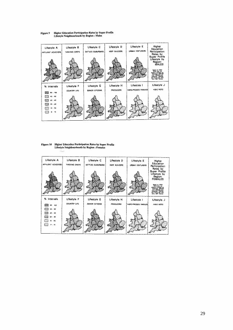
Figures 9 and 10 summarise the main geographical variations in the YEI, by Lifestyle
Neighbourhood. The maps show clearly the general decline in the participation rate,
across all regions, as one moves from more affluent to less affluent Lifestyle
Neighbourhoods. They also exhibit interesting inter-regional differentials which indicate
that the chances of attending university vary from one part of the country to another even
within the same type of residential area. In some regions (e.g. the North East) where the
overall YEI (see Figure 3) is relatively low, that amongst those living in the most affluent
residential areas is high, and vice versa. The maps also show that the regional
distribution of YEIs in the least affluent residential areas conform more closely to the
overall pattern of YEIs.
5. CONCLUSIONS
Several points are clear from this study. Among the factors investigated (gender, region
and geodemographic group), the most important in determining whether a young person
enters higher education is geodemographic group. The three lowest represented Lifestyle
Neighbourhoods (H, I and J) account for 30 per cent of the English eligible population
and have a YEI of 14 per cent, less than half the English mean. These areas are
characterised by low income, high unemployment and a high proportion of manual
workers. The two highest represented Lifestyle Neighbourhoods (A and B) make up 23
per cent of the English eligible population and have an YEI of 51 per cent, two thirds
higher than the English mean and over three times higher than the lowest represented
Lifestyle Neighbourhoods. These areas are characterised by high income, affluent
lifestyles and a high proportion of non-manual workers.

15
More detailed analysis of the results suggests that there is a positive correlation between
participation in higher education and affluence measured by income estimates.
The results obtained for the YEI are likely to be true of the API. This suggests that the
current value of the API of around 30 per cent should not be viewed as a natural
maximum but as a composite of very different rates.
Previous work implies that the variation of participation in higher education by social
group is closely related to educational achievement up to 18 years of age (Burnhill et al
1990; Pearson et al 1989). If the educational attainment of currently poorly performing
groups improved, then their rate of participation in higher education would be likely to
increase. Figure 11 illustrates the number of extra English YEI entrants who would have
entered higher education in 1994 if a certain minimum YEI is applied to the eligible
population at the Subgroup Area level. If all 40 Subgroup Areas had a minimum YEI of
30 per cent than the number of YEI entrants would increase by 35,000 to 204,000 (a 20
per cent increase) taking the YEI for England to 37 per cent.
The present study is exploratory and therefore should not be seen as a comprehensive
analysis of all aspects of variation in participation rates. It has examined cross-
sectional data from the mid-1990s in relation to full-time young entrants to higher
education. More work remains to be done on mature and part-time students, to establish
whether their pattern of participation matches that of young full-time students. It might
also be interesting to examine whether students in different subject areas or institutions
come from comparable backgrounds, or whether here too there is substantial variation in
participation by region, gender or residential neighbourhood type.
Given that the Dearing Committee has recommended a further expansion in student
numbers, it is particularly important that this study is followed up by regular monitoring
exercises that enable the YEI to be tracked over time. Some initial monitoring work is
currently underway. Data are being assembled for three subsequent years : 1995-96,
1996-97 and 1997-98. For this purpose HEFCE has supplied postcoded records of the
number of Young Entrants for each of the three years, with separate counts of males and
females. The denominator will be based on electoral roll records which specify date of

16
birth and gender of young people reaching the voting age of 18. Counts are available
from a commercial supplier, Equifax, by ED. This level of spatial disaggregation
provides considerable flexibility in deriving YEI statistics for other geographies at higher
levels of aggregation.
The annual counts, processed by ED, will enable a number of different measures of
change to be calculated, both from year to year and over a longer timescale. It will be
possible, for example, to estimate the differential change between years in terms of
absolute and percentage change in numbers by Target Market or Lifestyle, by region.
Such rates of change by region can also be translated into indices which compare the
regional rate with the overall national rate of change in participation; a region matching
the national average would be set to 100. In this way it should be possible to establish
which regions (and which Lifestyle Neighbourhood or Subgroup Area) are leading or
lagging behind national growth rates.
A variant on this form of change analysis would indicate the period of time over which a
region (or geodemographic category) could be expected to take to enable it to match, or
converge with, either the national average YEI or, more usefully, a specified target rate of
participation, such as 35 per cent. Such a measure could be termed the ‘implied
convergence time’ for the region (or geodemographic category), given the current rate of
change in the YEI.
Finally, it is worth noting that the Dearing Committee has explicitly endorsed the area-
based approach to examining participation rates. One of its recommendations urges the
higher-education funding bodies “to consider financing, over the next two or three years,
pilot projects which allocate additional funds to institutions which enrol students from
particularly disadvantaged localities” (National Committee of Inquiry into Higher
Education : Summary Report, 1997, p.42, Recommendation 4). This paper has gone
some way towards indicating how such a recommendation might be put into effect.

17
REFERENCES
Batey, P.W.J. and Brown, P.J.B. (1995) From Human Ecology to Customer Targeting:the Evolution of Geodemographics, P. Longley and G.Clarke (eds.) GIS for Business andService Planning, Longman. London. pp. 77-103.
Brown, P.J.B. and Batey, P.W.J. (1994a) Design and Construction of ageodemographic Targeting System: Super Profiles 1994, URPERRL Working Paper 40,Department of Civic Design, University of Liverpool, 52 pp.
Brown, P.J.B. and Batey, P.W.J. (1994b) Characteristics of Super Profile Lifestylesand Target Markets: Index Table and Pen Picture Descriptions, and GeographicalDistribution Super Profile Technical Note 2, URPERRL-Liverpool, Department of CivicDesign, Liverpool, 79pp.
Burnhill, P., Garner, C. and McPherson, A. (1990) Parental Education, Social Classand Entry to Higher Education 1976-86, J.R. Statist. Soc. A, 153, Part 2, pp. 233-248.
DES (1986), Technical Report to DES Report on Education 100 (Demand for HigherEducation in Great Britain 1984-2000).
The Economist (1997) A Survey of Universities : The Knowledge Factory Specialsupplement, October 4, 1997.
Egerton, M. and Halsey, A.H. (1993) Trends by Social Class and Gender in Access toHigher Education in Britain Oxford Review of Education Vol. 19, No. 2, pp. 183-195.
Higher Education Funding Council for England (1996) Widening Access to HigherEducation, 9/96, HEFCE.
Metcalf, H. (1993), Non-traditional Students’ Experience of Higher Education: AReview of the Literature, Policy Studies Institute, CVCP Briefing.
National Committee of Inquiry into Higher Education (1997) Higher Education inthe Learning Society : Summary Report.
Pearson, R., Pike, G., Gordon, A. and Weyman, C. (1989) How Many Graduates inthe 21st Century? - The Choice is Yours, IMS Report No. 177, Institute of ManpowerStudies, University of Sussex.
Robertson, D. and Hillman, J. (1997) Widening Participation in Higher Educationfrom Lower Socio-Economic Groups and Students with Disabilities, Report 6, NationalCommittee of Inquiry into Higher Education, London.
Royal Statistical Society (1985), Projections of Student Numbers in Higher Education,J.R. Statist. Soc. A, 148, Part 3, pp. 175-213.
Tonks, D.G. and Farr, M. (1994) ‘Market Segments for Higher Education : Using
Geodemographics’ Marketing Intelligence and Planning 13(4), pp. 24-33.

18
Appendix 1
Age Participation Index
Students eligible for the numerator of the Great Britain API are defined as home (UnitedKingdom) domiciled students aged under 21 years on 31 December of the year of entry,entering a course of full-time undergraduate level higher education for the first time inGreat Britain. Note this includes United Kingdom students attending institutions inGreat Britain (therefore excluding, for example, English students attending highereducation courses in Northern Ireland), counts full-time entrants only and includes highereducation undertaken in further education colleges. Students from the Channel Islandsand the Isle of Man are counted for the numerator of the GB API but their population isnot included in the denominator.
In recent times API student information was obtained from separate statistical records:
a. The Universities Statistical Records (USR), for the former Universities Funding Council funded universities.
b. The Further Education Statistical Record (FESR), for the former Polytechnics and Colleges Funding Council funded institutions.
c. The FESR analogues run by the Welsh and Scottish Offices.
The differences in data definitions between these records introduced complications. Forinstitutions formerly recorded in the USR, the census date for the student count is 31December and courses less than 9 months long are excluded. For institutions recordedon the FESR, the census date is 1 November. Additionally for former PCFC-fundedinstitutions the number of students not on initial teacher training courses are reduced by13 per cent (this being an estimate of the number of those students who have alreadybeen exposed to higher education).
The eligible population is taken as the mean of 18 year olds and 19 year olds on 31December of the year of entry. This information is derived from Government populationestimates.
YEI: Eligible Students
The present study investigates students who entered higher education (in highereducation institutions) for the first time in the academic year 199495. HESA providestwo student records for this academic year, relating to information collected in theautumn and summer. To obtain the numerator for the YEI students were selected fromthe July student record for 1994-95 in a manner similar, but not identical, to the DfEEAPI definition. Students were selected for the YEI count if they satisfied all thefollowing criteria:
* home student (not Channel Islands or Isle of Man)
* under 21 years of age at 31 December 1994

19
* full-time course only
* undergraduate level
* new entrant (this was defined using a HESA flag variable that marks students in their first year who do not have higher education qualifications on entry)
* entering institution on or before 1 December 1994
* attending United Kingdom higher education institutions
Note that these criteria differ from those used in the GB API. The main differences arethat Northern Ireland higher education institutions are included for the YEI and highereducation students in further education establishments, and those from the ChannelIslands and Isle of Man, are excluded.
Students attending Northern Ireland institutions were included because it was thoughtthat excluding them would not affect all regions equally. This would then make itdifficult to establish whether there was any regional variation in participation.
The correction for students changing courses (a deduction of 13 per cent from thenumber of non-initial teacher training students in institutions formerly funded by thePCFC) has been replaced by using the new entrant flag. It is not certain that the 13 percent adjustment is still an accurate reflection of numbers changing course in the formerPCFC institutions. Previous work has suggested that participation by the manual socialgroups is relatively low, and also that the students from these groups are concentrated informer PCFC funded institutions. By not applying the deduction the study probablygives an optimistic estimate of the number of students from these groups.
A small proportion of higher education is provided by the further education sector.These students have been excluded from this study because postcode information was notreadily available for them.
YEI: Estimating the Eligible Population
The calculations to provide the denominator for the YEI should provide figures close tothose used by the API, though approximations have been made (mainly because of therequirement to have population estimates by age for each enumeration district).
The project makes use of data from the Small Area Statistics. At the enumeration districtlevel this is tabulated as a count of 15 year olds and a count of 16/17 year olds. For thisproject a simple estimate of the 16 year olds was obtained by taking half the 16/17 yearold count. The resulting estimate of 15 year olds and 16 year olds is taken to be the sameas the number of 18 year olds and 19 year olds at the 31 December 1994 (the eligiblepopulation for the YEI statistic). The necessity to obtain census data at the enumerationdistrict level introduces two significant approximations which are described in thefollowing paragraphs.

20
The number of live births in England fell each year from 685,000 in 1973 to 550,000 in1976. By taking half the 16 and 17 year old count in 1991 as an approximation to thenumber of 16 year olds will exaggerate this number (as there are fewer 16 year olds than17 year olds in reality because of the falling number of births).
The API statistic measures age at 31 December in the year of entry. The ages recorded inthe Small Area Statistics are those at the census date (21 April 1991). Therefore, forentry in 1994, the API statistic (and the YEI) counts students born between 1 January1975 and 31 December 1976. By using the census dates the project will be estimatingthose born between 22 April 1974 and 21 April 1976, a cohort 8 months older than theintended one. This will act to inflate the estimates of 18 and 19 year olds in 1994because of the falling number of births.
Approximate calculations using annual birth totals for England (and assuming a constantdecline in the number of births) suggest that together these two approximations will actto inflate the estimate of 18 and 19 year olds used in this project by around 6 per cent.
The inflation of the estimate is probably partly offset by not accounting for the growthnormally observed in English cohorts as they age from 15 year olds to 19 year olds (duemainly to inward migration). This is typically 2,500 a year (amounting to almost 10,000,around 2 per cent, over the ageing period). Additionally, the exclusion of the 1-2 percent of areas not covered by the classification system will act to deflate the English totalpopulation estimate (but will not affect the value of the YEI because the student countsare affected in the same way).

21
Figures and Tables
Figure 1 Age Participation Index for Great Britain 1972-94
Figure 2 Eligible Students and Weighted Students by Region
Figure 3 Youth Entrant Index by Region
Figure 4 YEI Eligible Population and Weighted Studentsby Lifestyle Neighbourhood
Figure 5 YEI by Lifestyle Neighbourhood
Figure 6 YEI by Estimated Household Income of Subgroup Area
Figure 7 Distribution of Gender YEI Ratios
Figure 8 Observed and Adjusted YEI by Region
Figure 9 Higher Education Participation Rates by Super Profile Lifestyle Neighbourhoods by Region : Males
Figure 10 Higher Education Participation Rates by Super Profile Lifestyle Neighbourhoods by Region : Females
Figure 11 Potential Extra English Young Entrants ofSubgroup Areas Subjected to a Minimum YEI
Table 1 Selected Characteristics of Lifestyle Neighbourhoods
Table 2 Super Profile Subgroup Areasby Lifestyle Neighbourhood

22

23

24

25

26

27

28
29

30

31