participation in the panel mdps: ai versus or workshop on

Participation in the PanelMDPs: AI versus OR

Workshop on Decision Making inAdversarial Domains

Greenbelt, MDEugene A. Feinberg

[email protected]

Department of Applied Mathematics and Statistics

State University of New York at Stony Brook

Participation in the PanelMDPs: AI versus ORWorkshop on Decision Making in Adversarial DomainsGreenbelt, MD – p. 1/25

Markov Decision Process (MDP)

I: state space;

A: action space;

A(i): action set available at state i;

p(i, a, j): transition probabilities;

rk(i, a): one-step rewards.

For a stationary policy, a selected action depends only onthe current state. We also consider randomized stationarypolicies. General policies may be randomized and dependon the past.


IntroductionConsider a problem with K + 1 criteria

W0(π),W1(π), . . . ,WK(π), where π is a policy. A natural

approach to dynamic optimization is

maximize W0(π)

subject to

Wk(π) ≥ Ck, k = 1, . . . ,K.

For K > 0 this approach typically leads to the optimality of

randomized policies with the number of randomizations is

limited by the number of constraints.

For unconstrained problems (K = 0) there exists a

nonrandomized stationary policy. This policy is usually optimal

for all initial states.


Performance CriteriaThe most common criteria are:

Expected total rewards over the finite horizon.

Average rewards per unit time.

Expected total discounted rewards.

Let rk(i, a) be the one-step reward for criterion k if an actiona is used in state i.

Expected total rewards over N steps:

Wk(i0, π,N) := Eπi0

N−1∑

t=0

rk(it, at),

where i0 is the initial state and π is the policy.


Performance Criteria: Continuation

Average rewards per unit time:

Wk(i0, π) := lim infN→∞

Wk(i0, π,N)

N.

Total discounted rewards:

Wk(i0, π) := Eπi0

∞∑

t=0

βtrk(it, at),

where β ∈ [0, 1) is a discount factor.

In some problems, the initial state is given by an initialdistribution µ. Similar criteria can be considered forcontinuous-time problems.


LP Formulation

maximize∑

i∈I

∑

a∈A(i)

r0(i, a)xi,a

subject to∑

a∈A(j)

xj,a − β∑

i∈I

∑

a∈A(i)

p(j, a, i)xi,a = µ(j), j ∈ I,

∑

i∈I

∑

a∈A(i)

rk(i, a)xi,a ≥ Ck, k = 1, . . . ,K,

xi,a ≥ 0, i ∈ I, a ∈ A(i).


Optimal policy

φ(a|i) =

xi,a/∑

b∈A(i)

xi,b, if the denominatior is positive;

arbitrary, otherwise.

Interpretation: xi,a are so-called occupation measures,

xi,a = Eφµ

∞∑

t=0

βtI{it = i, at = a}.

For average rewards per unit time, xi,a are state-action frequencies,

xi,a = limN→∞

1

NE

φµ

N−1∑

t=0

I{it = i, at = a}.


Number of RandomizationsLet Rand(φ) be the number of randomizations for arandomized stationary policy φ,

Rand(φ) =∑

i∈I

{−1 +∑

a∈A(i)

I{φ(a|i) > 0}}.

ThenRand(φ) ≤ K, (1)

where K is the number of constraints.

For finite I, (1) follows from the LP arguments ( Ross1989).

For countable I: F & Shwartz (1996) (Borkar 1992 foraverage rewards per unit time).

For uncountable I: an open problem.Participation in the PanelMDPs: AI versus ORWorkshop on Decision Making in Adversarial DomainsGreenbelt, MD – p. 8/25

Constrained MDPs and problems in adversarial domains

Constrained MDP is a nice model for problems inadversarial domains because of optimality ofrandomized policies. It is natural for problems inadversarial domains to keep the randomization index aslarge as possible.

This leads to new problem formulations.


F’s current research directions relevant to MDPs

Continuous time MDPs;

Non-atomic discrete-time MDPs;

Applications to inventory control, discrete optimization,queueing control, ...


Continuous time MDPsThe time is continuous and an action a selected in statei defines a vector of transition intensities q(i, a, j) ≥ 0,i 6= j.

Let q(i, a) =∑

j 6=i q(i, a, j).

If q(i, a) = 0 then i is an absorbing state.

Otherwise, the system spends on average q−1(i, a) unitsof time in state i and then moves to j 6= i with theprobability p(i, a, j) = q(i, a, j)/q(i, a).

There are reward rates rk(i, a) when the system stays instate i and instant rewards Rk(i, a, j) when the systemjumps from state i to state j.

Major motivation: control of queues and queueingnetworks.


Continuous time MDPs: Switching policies

Let x be the LP solution andAx(i) = {a ∈ A(i) : xi,a > 0} = {a(i, 1), . . . , a(i, n(i, x))}.

Let S0(i, x) = 0. For ℓ = 1, . . . , n(i, x), we set

sℓ(i, x) = −(α+ q(i, a(i, ℓ)))−1 ln(1 − xi,a(i,ℓ)/

n(i,x)∑

j=ℓ

xi,a(i,j)),

and Sℓ(i, x) = Sℓ−1(i, x) + sℓ(i, x).

Optimal switching stationary policy ψ:

ψ(i, t) =

a(i, ℓ), if Ax(i) 6= ∅ and Sℓ−1(i, x) ≤ t < Sℓ(i, x);

arbitrary action a, if Ax(i) = ∅.


Optimality of switching policiesChange of intensity between jumps is equivalent torandomized decisions at jump epochs.

Consider two independent Poisson arrival processes 1or 2 with positive intensities λ1 and λ2.

At each epoch t ∈ [0,∞[, an observer can watch eitherprocess 1 or 2. The process stops when the observersees an arrival.

A policy π is a measurable function π : [0,∞[→ {1, 2}.

Let pπi , i = 1, 2 be the probability that the first

observed arrival belongs to process i.Let ξ be the time when an observer sees an arrivalfor the first time. In other words, pi = P{π(ξ) = i}.


Optimality of switching policiesLet ξi be the time that process i has been watched beforethe first detected arrival, ξ = ξ1 + ξ2,

ξi =

∫ ξ

0I{π(t) = i}dt.

Lemma 1 pi = λi E ξi.

Remark 1 pi and E ξi depend on the policy π

Remark 2 If π(t) = 1 for all t, we get E ξ1 = 1λ1

- themean of an exponential random variable.

Selecting intensities λ1 and λ2 randomly with theprobabilities p1 and p2 respectively yields the same averagecharacteristics as selecting intensity λ1 during timeT = −λ−1

i ln(1 − p1) and then switching to λ2.


Non-Atomic MDPsIf the state space is uncountable, we denote it by Xinstead of I. In this case, we use the notation px,a(Y )

instead of p(i, a, j). Let the initial distribution µ andtransition probabilities px,a be non-atomic; i.e. µ(x) = 0

and px,a(y) = 0 for all states x, y and for all actions a.

Then for any policy π there exists a deterministic policyφ such that Wk(µ, φ) = Wk(µ, π), k = 0, 1, . . . ,K.

F and Piunovskiy (2002, 2004).

Examples of applications:Statistical decision theory (Dvoretzky, Wald, andWolfowitz 1951, Blackwell 1951).Inventory control.Portfolio management.


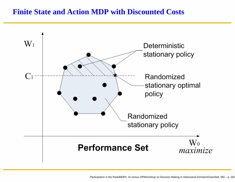
Finite State and Action MDP with Discounted Costs


Explanation


Nonatomic MDP with Discounted Costs


Deterministic Statistical DecisionsX: Borel state space;

A: Borel action space;

µn, n = 1, . . . , N : non-atomic initial probabilities on X;

ρ(µn, x, a) : costs.

W (µ, π) =

∫

X

∫

A

ρ(µn, x, a)π(da|x)µn(dx).

Dvoretzky, Wald, and Wolfowitz (1951): If A is finite, forany π there exists a deterministic decision rule φ suchthat

(W (µ1, φ), . . . ,W (µN , φ)) = (W (µ1, π), . . . ,W (µN , π)).

F & Piunovskiy (2004): A could be arbitrary.


Other OR/AI approachesNeuro-Dynamic Programming

Perturbation analysis

We need more applications to test and comparedifferent approaches

A possible military-relevant application to test variousapproaches is the Generalized Pinwheel Problem


Motivation for the Generalized Pinwheel Problem


Generalized Pinwheel ProblemThe radar sensor management problem can be formulatedin general terms.Consider the following infinite-horizon non-preemptivescheduling problem:

There are N jobs. Each job i, i = 1, . . . , N ischaracterized by two parameters:

τi, the duration of job i,ui, the maximum amount of time between instanceswhen job i is completed and started again.


Generalized Pinwheel ProblemA schedule is feasible if each time job i is performed, itwill be started again no more than ui seconds after it iscompleted.

Our goal is to find a feasible schedule or conclude that itdoes not exist.


Generalized Pinwheel ProblemThis problem is NP-hard but a good heuristic is a so-calledFrequency-Based Algorithm (F & Curry, 2005):

Consider a relaxation,

Formulate an MDP for this relaxation,

Find optimal frequencies by solving this LP,

Find a time-sharing policy (sequence),

Try to cut a feasible piece of this sequence.


Time-Sharing PoliciesLet I and A be finite and let stationary policies define recurrent

Markov chains. Let xi,a be the vector of optimal state-action

frequencies and φ is the corresponding randomized stationary

optimal policy. For any finite trajectory x0, a0, . . . , xn−1, define

Nn(i, a) =

n−1∑

t=0

I{xt = i, at = a},

Nn(i) =

n−1∑

t=0

I{xt = i},

δ(i, n) = argmaxa∈A(i){xi,a −Nn(i, a) + 1

Nn(i) + 1}.

Then policies φ and δ yield the same performances.


participation in the panel mdps: ai versus or workshop on

Documents