particle dynamics and sinking rates of the marine diatom skeletonema costatum · 2011-05-31 ·...
TRANSCRIPT
PARTICLE DYNAMICS ANDSINKING RATES OF THE MARINE DIATOM
Skeletonema costatum
Daniel Meunier
2001
Department of Environmental EngineeringCentre for Water Research
University of Western AustraliaNedlands, W.A., 6097, AUSTRALIA

- i -
ABSTRACT
The distribution of marine phytoplankton, and marine diatoms in particular, is of major
importance to global climate and primary production. The changes in the distributions of these
diatoms is strongly controlled by their sinking rates (Smayda, 1970). Therefore, sinking rates of
diatoms have been measured in both the laboratory and in the field by many methods.
The relationship between particle size and particle sinking rate is important for our understanding
of the biological and physical controls of this vertical flux. This relationship is also used by
modelers to predict particle export from surface waters. A new method for determining the
sinking rates of marine diatoms has been developed by A. Waite and K. O’Brien at the Centre for
Water Research (CWR) at the University of Western Australia (UWA). This method uses the
concept of non-disruptive observation of sinking particles as developed by Waite et al. (1997).
Past methods for determining sinking rates of marine diatoms include the SETCOL as developed
by Bienfang (1981).
We investigated the effect of nutrient limitation on the size versus sinking rate relationship using
both methods, on the marine diatom Skeletonema costatum, and the aggregates formed of this
species. Aggregation was induced by a shear on nitrogen depleted cultures.
Stokes’ Law has commonly been applied to the sinking of marine phytoplankton. The
applicability of Stokes’ Law to a range of single chain and aggregates of Skeletonema costatum
was tested. The results showed that sinking rate was proportional to the equivalent diameter of a
given chain or aggregate (ws ∝ d). This did not did not confirm earlier work that suggested that
sinking rate is proportional to the square of the diameter (ws ∝ d2).
Hutchinson (1967) had introduced a coefficient for the form drag of a particle or aggregate into
Stokes’ Law, the effect of this coefficient was clearly applicable to the data obtained. Reynolds
(1984) and Waite et al. (1992a) also found that sinking rate of diatoms is proportional to the
diameter. Skeletonema costatum is known to be affected by drag via its cell-cell linkage. We
suggest that changes in drag can occur as the result of changes in physiological state, the shape of
individual cells, cells in aggregates, as well as the shape and porosity of these aggregates.

ACKNOWLEDGEMENTS
- ii -
ACKNOWLEDGEMENTS
This thesis is the final product of one years work, that has been hard but also enjoyable. I would
not have been able to complete this project without the support of my family and friends.
I would like to thank my supervisor, Anya Waite, for providing me with a project that was ‘hands
on’. I would like to thank Anya for giving up time from her study leave to assist me via Email.
I would like to thank David Hamilton, for his assistance in Anya’s absence during the second
semester of this year.
I would especially like to thank Bridget Alexander for her assistance with the laboratory work
completed and her technical knowledge provided.
I would also like to acknowledge the assistance Kate O’Brien provided me throughout the year.
I would like to dedicate this thesis to the memory of my father, Guy Meunier, who was
inspirational in making me the person I am today.
Daniel Guy Meunier
TABLE OF CONTENETS
- iii -
TABLE OF CONTENTS
ABSTRACT………………………………………………………………………...i
ACKNOWLEDGEMENTS……………………………………………………….ii
TABLE OF CONTENETS……………………………………………………….iii
INDEX OF TABLES AND FIGURES…………………………………………...v
1 INTRODUCTION……………………………………………………………….1
2 LITERATURE REVIEW……………………………………………………….3
2.1 MARINE PHYTOPLANKTON: DIATOMS………………………………………………32.1.1 CELL STRUCTURE………………………………………………………………...32.1.2 PHOTOSYNTHESIS AND PHOTORESPIRATION………………………………52.1.3 REPRODUCTION……………………………………………………………….….62.1.4 DIATOM SPORES AND RESTING CELLS……………………………………….7
2.2 THE BIOLOGICAL PUMP AND THE GLOBAL CARBON CYCLE………………….72.3 PHYTOPLANKTON SINKING RATE……………………………………………….…....9
2.3.1 SINKING RATE MEASUREMENT……………………………….……………...112.3.2 FACTORS AFFECTING SINKING RATE……………………….……………....14
2.4 AGGREGATION……………………….……………..……………………………………142.4.1 CAUSES OF AGGREGATION: OBSERVATIONS……………………………...152.4.2 FORMATION OF AGGREGATES…………………………….………………….152.4.3 AGGREGATION QUANTIFICATION METHODS……….……………………..16
3 METHODOLOGY……………………………………………………………..19
3.1 CULTURING………………………………………………………………………………..203.1.1 INOCULATION……………………………………………………………………203.1.2 CULTURING CONDITIONS……………………………………………………...203.1.3 NITROGEN LIMITATION…………………………………………………….….253.1.4 REPLICATION AND INOCULATION OF 20L CULTURES……………….…...273.1.5 GROWTH RATE MEASUREMENT……………….….………………………….27
3.2 AGGREGATION…………………………………………………………………………...283.2.1 THE ROLLER TABLE……………….….………………………………………...283.2.2 TEP MEASUREMENTS…………….….………………………………………....29
3.3 SINKING RATE MEASUREMENT………………………………………………….…...293.3.1 SETCOL………………………………………………….….……………………..293.3.2 VIDEO OBSERVATION………………………….….…………………………...30
3.4 PARTICLE SIZES………………………………………………….….…………………...343.4.1 COULTER COUNTER……………………………….….………………….……..343.4.2 MATLAB……………………………….….………………….…………………...34

TABLE OF CONTENETS
- iv -
4 RESULTS……………………………………………………………………….36
4.1 GROWTH RATE……………………………………………….….………………….……364.1.1 RAW FLUORESCENCE……...……………………….….………………….……364.1.2 CHLROPHYLL a………………………….….………………….………………...374.1.3 COULTER COUNTER CELL COUNT…………….……………….…………….38
4.2 NITROGEN LEVELS………………………….….………………….…………………….384.3 AGREGATION……….….………………….……………………………………………...39
4.3.1 TEP MEASUREMENTS.…………………………………………….……………394.4 SETCOL SIZE AND SINKING RATES….…………………………………………….…40
4.4.1 SETCOL NON-AGGREGATED SINKING RATES…………………….………..404.4.2 SETCOL AGGREGATED SINKING RATES…………………….………………404.4.3 COULTER COUNTER CELL SIZE DISTRIBUTIONS…………………….……41
4.5 VIDEO OBSERVATION RESULTS……………………………………………………...42
5 DISCUSSION…………………………………………………………………..44
5.1 VIDEO OBSERVATION…………………………………………………………………...445.2 SETCOL………………………………………………………………….………………….49
6 CONCLUSIONS………………………………………………………………..50
REFERENCES…………………………………………………………………...51
Appendix I……………………………………………………………………………………….57
Appendix II……………………………………………………………………………………...58
Appendix III……………………………………………………………………………………..59
Appendix IV……………………………………………………………………………………..61
Appendix V………………………………………………………………………………………62
Appendix VI……………………………………………………………………………………..64
INDEX OF TABLES AND FIGURES
- v -
INDEX OF TABLES AND FIGURES
Figure 2.1.1: Section showing epitheca and hypotheca…………………………………………3Figure 2.1.2: Coscinodiscus sp. an example of a centric diatom. Scale bar = 40µm. Achnanthes
taeniata an example of a pennate diatom. Scale bar = 20µm…………………………………….4
Figure 2.1.3: Skeletonema costatum a chain forming marine diatom. Scale bar = 4µm. Cells can
be seen as marked, with hairlike protrusions joining them……………………………………….4Figure 2.1.4: Illustration of simultaneous gross photosynthetic CO2 fixation by the C3 cycle andphotorespiration by the C2 cycle (Tolbert & Preiss, 1994)……………………………………….6Figure 2.2.1: Schematic diagram of the biological pump in the ocean…………………………..8Figure 2.2.2: Simplified scheme of the main pools and fluxes of carbon between the atmosphere,biosphere and geosphere. The size of each is given in giggatonnes of carbon (GtC). The fluxesare also in GtC. The CO2 concentration in the atmosphere is shown as volumes per volume(equivalent to volume parts per million (vpm)) or as partial pressure (Pa) (Lawlor, 2001)………8Figure 2.3.1: SETCOL instrument as developed by Waite et al (1997). Consisting of foursymmetric columns (1, 2, 3 & 4) immersed in a water bath, with outlets for the columns at thetop, middle and bottom…………………………………………………………………………...13Figure 2.3.2: Plan view of setup of video monitoring of sinking rate…………………………...13Figure 2.4.1: Schematic of flocculation device and video set up………………………………..17Figure 3.1.1: Points along the growth rate curve where major sinking rate and aggregationexperiments were performed……………………………………………………………………..19Figure 3.1.2: The timing device used to turn the lighting on and off……………………………21Figure 3.1.3: The lighting system for culturing. The two replicate 20 litre carboys can be seen aswell as the 50 mL test tubes. During culturing the second rack is positioned in front of the twocarboys……………………………………………………………………………………………22Figure 3.1.4: Positions of light meters for light level measurement…………………………….23Figure 3.1.5: Fluid motion in large 20L carboy.………………………………………………...25Figure 3.1.6: Growth rate curves of limited cultures, as measured by raw fluorescence………..26Figure 3.1.7: Graphical representation of Equation 3.1.1……………………………………….27Figure 3.1.8: Roller table with 2 litre SCHOTT bottle rotating on top. The creation of a shearwithin the bottle can be seen with maximum velocity at the sides of the bottle and minimumvelocity in the centre……………………………………………………………………………..29Figure 3.3.1: Schematic view of column into which the culture is diffused and the light source.The camera would be positioned looking into the column from this position…………………..30Figure 3.3.2: Example of MATLAB image of micrometer, showing 15 lines to be considered inthe calibration (lines 1 and 15 are labeled). The x and y lengths are shown……………………..31Figure 3.3.3: An example of the image created when overlaying frames. The real image has beencropped from the sides……………………………………………………………………………32Figure 3.3.4: An example of the points used to determine sinking rate (green circles), and thetotal displacement. The edges of the green box surrounding the aggregate are the limits of thearea within which the size of the aggregate is determined. This image total has been cropped…33Figure 4.1.1: The growth rate curves of the three previous ‘healthy’ generations of SkeletonemaCostatum prior to inoculation of the 20 L replicates……………………………………………..36Figure 4.1.2: Comparison of fluorescence and chlorophyll a concentration over the course ofexperimentation…………………………………………………………………………………..37Figure 4.1.3: Comparison of fluorescence and cell counts over the course of experimentation...38Figure 4.1.4: TEP measurements over the course of experimentation for both replicatecultures……………………………………………………………………………………………39

INDEX OF TABLES AND FIGURES
- vi -
Table 3.1.1: The results of the LI-COR Photometer and the Digital Lux Meter. Using theconversion rate of 1 klux = 12 µE………………………………………………………………..23
Table 4.1.1: Daily fluorescence reading s for both replicates, named Culture 1 and Culture 2,respectively.………………………………………………………………………………………37Table 4.2.1: Dissolved nitrogen levels for both replicates over the course of experimentation.Values are in µg.N/L. ……………………………………………………………………………39
Table 4.4.1: Sinking rates for replicate culture 1 for both columns of the SETCOL..…………..40Table 4.4.2: Sinking rates for replicate culture 2 for both columns of the SETCOL..…………..40Table 4.4.3: Sinking rates for aggregated volumes of replicate culture 1 for both columns of theSETCOL………………………………………………………………………………………….41Table 4.4.4: Sinking rates for aggregated volumes of replicate culture 2 for both columns of theSETCOL………………………………………………………………………………………….41Table 4.4.5: Particle size statistics for both replicate cultures…………………………………...42Table 4.4.6: Non-aggregated volumes diameter ranges (µm).…………………………….…….42
Table 4.4.7: Non-aggregated volumes sinking rate ranges (m day-1).…………………………...42Table 4.4.8: Aggregated volumes diameter ranges (µm)………………………………………..43
Table 4.4.9: Aggregated volumes sinking rate ranges (m day-1)………………………………...43Table 4.4.10: The number of particles identified in each test. Values in brackets represent totalparticle numbers when combining the relative sets of data………………………………………43Table 5.1.1: The form resistance values over the lifecycle of Skeletonema costatum…………..49

CHAPTER 1 INTRODUCTION
- 1 -
1 INTRODUCTION
The distribution of marine phytoplankton and in particular marine diatoms is of major importance
to global climate. The changes in distribution of these diatoms are controlled strongly by their
sinking rate to depths were they can no longer be active in the process termed the ‘biological
pump’. Marine diatoms will sink out of the photic zone of the ocean for several reasons. One of
these reasons is nutrient depletion. This removal of photoautotrophic biomass is a major loss to
the primary production resource of the oceans, it is also a potential loss of atmospheric CO2 due
to the action of the ‘biological pump’.
The ‘biological pump’ describes the removal of CO2 from the atmosphere by means of
photosynthesis by marine phytoplankton (including diatoms). The determination of the rates at
which these diatoms sink is of great importance in determining the rate of loss of these
phytoplankton and their effect on the global climate.
Several laboratory experiments have been developed, in time, to determine the rates of sinking of
these microscopic particles, as well as the sinking rates of the aggregates that they form. Methods
developed include the SETCOL (Bienfang et al., 1981) and the MARS instrument (Bienfang et
al., 1978).
The ‘stickiness’ or rate of aggregation of marine diatoms had been a topic of much research.
Several methods have been developed to elucidate this effect. The most effective and least
intrusive method of determining the ‘stickiness’ of the particles is by the video analysis of
flocculator images (Waite et al., 1997a).
The aim of this thesis was to determine the sinking rates of aggregates formed by nitrogen limited
cultures of the marine diatom Skeletonema costatum. The sinking rates of individual particles of
this species of marine diatom have been conducted previously (e.g. Waite et al., 1997b) but few
studies have been done on the larger aggregates formed from laboratory culturing.

CHAPTER 1 INTRODUCTION
- 2 -
Several outcomes are expected of this thesis:
• To determine the applicability of Stokes’ Law of sinking to the aggregates of the marine
diatom Skeletonema costatum.
• To determine the accuracy and relevance of the new Video Observation method for
sinking rate determination.
• To develop a methodology that can be applied to other marine diatoms.
The process by which these aims are achieved and the outcomes of experimentation are outlined
in the following sections of this thesis.

CHAPTER 2 LITERATURE REVIEW
- 3 -
2 LITERATURE REVIEW
2.1 Marine Phytoplankton: Diatoms
Diatoms are unicellular plants belonging to the plant class Bacillariophyceae of the phylum
Chromophyta (Tomas, 1996). Diatoms dominate the phytoplankton of cold nutrient rich waters,
such as upwelling areas of the oceans, and recently circulated lake waters (Graham & Wilcox,
2000). They are ubiquitous, occurring in marine and fresh waters, where they may be planktonic,
benthic, periphytic (growing on plant or seaweed surfaces) or epizoic (on animals). Some species
are capable of active movement but others depend on currents for transport. Individual diatoms
range in size from 2 µm to several millimetres, although there are very few species that are larger
than 200 µm. The actual number of extinct and extant diatom species may well be over 50,000
(Tomas, 1996).
2.1.1 Cell Structure
Diatoms are characterised by a skeleton, or capsule, the frustule, which is composed of the
epitheca and the hypotheca, that fit together (McConnaughey, 1970) (Figure 2.1.1). These valves
are impregnated with silica, which gives them a glasslike character (McConnaughey, 1970). The
two theca are held together by what is termed the girdle. The valves are transparent and usually
beautifully and symmetrically ornamented with a variety of markings. There are two common
shapes; centric and pennate (Figure 2.1.2). The centric diatoms are typically discoid or cylindrical
cells that have radial symmetry in face or ‘valve’ view. In contrast, valves of pennate diatoms
have more or less bilateral symmetry. Some pennate diatoms possess slits in the frustule – the
raphe system – that are associated with the ability to accomplish rapid gliding motion (Graham &
Wilcox, 2000).
CHAPTER 2 LITERATURE REVIEW
- 4 -
Figure 2.1.1: Section showing epitheca and hypotheca.
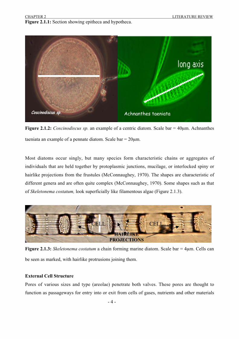
Figure 2.1.2: Coscinodiscus sp. an example of a centric diatom. Scale bar = 40µm. Achnanthes
taeniata an example of a pennate diatom. Scale bar = 20µm.
Most diatoms occur singly, but many species form characteristic chains or aggregates of
individuals that are held together by protoplasmic junctions, mucilage, or interlocked spiny or
hairlike projections from the frustules (McConnaughey, 1970). The shapes are characteristic of
different genera and are often quite complex (McConnaughey, 1970). Some shapes such as that
of Skeletonema costatum, look superficially like filamentous algae (Figure 2.1.3).
Figure 2.1.3: Skeletonema costatum a chain forming marine diatom. Scale bar = 4µm. Cells can
be seen as marked, with hairlike protrusions joining them.
External Cell Structure
Pores of various sizes and type (areolae) penetrate both valves. These pores are thought to
function as passageways for entry into or exit from cells of gases, nutrients and other materials
Achnanthes taeniata
HAIRLIKEPROJECTIONS
CELLCELL
CHAPTER 2 LITERATURE REVIEW
- 5 -
(Graham & Wilcox, 2000). The pores are usually complex and often have a silicified layer
(known as a velum) penetrated by smaller pores or slits stretched over them.
Many centric diatoms (and many pennate diatoms without raphe systems) possess a rimoportula,
a tubular structure that passes through the valve, ending on the inside in a slit, as if the tube were
laterally compressed (Graham & Wilcox, 2000). This structure is known as a labiate process and
is associated with polysaccharide mucilage secretion (Medlin et al., 1986). The other type of
mucilage secretion structure seen in centric diatoms is the ocellus. This is an elevated plate of
silica that is perforated by pores and surrounded by a rim.
Internal Cell Structure
The cytoplasm forms a relatively thin lining along the inside walls of the valves, surrounding a
vacuole filled with cell sap (McConnaughey, 1970). Within this cytoplasm is the protoplast
which contains several other components of the diatom. The nucleus has cytoplasmic strands
extending from it to other parts of the cell (McConnaughey, 1970). The cytoplasm, which
contains chloroplasts, the sites of photosynthesis (McConnaughey, 1970). The brownish colour
characteristic of most diatoms is caused by the pigment diatomin which is present in the
chloroplasts (McConnaughey, 1970).
2.1.2 Photosynthesis and Photorespiration
Photosynthesis is the process by which algae (and other photoautotrophs) convert the energy of
light into the chemical energy of organic molecules (Lawlor, 2001). One of the major factors in
controlling atmospheric CO2 and O2 is photosynthetic CO2 fixation and photorespiratory CO2
release by algae (Tolbert & Preiss, 1994). Most organisms now living on our globe depend on the
organic matter produced by photoautotrophs (Nielsen, 1975). In the sea, at least in all oceans,
phytoplankton are by far the most important vegetation (Nielsen, 1975).
Photosynthesis occurs in the presence of light in a region known as the photic zone. This zone is
strictly defined as the deepest depth in which the rate of photosynthesis is greater than the rate of
respiration over a daily cycle.
Diatoms have accessory photosynthetic pigments known as carotenoids. This makes it possible
for them to carry out photosynthesis over a broad range of wavelengths from 350 to 700 nm.
CHAPTER 2 LITERATURE REVIEW
- 6 -
The large surface area to volume ratio of phytoplankton enables efficient uptake of nutrients
(Nielsen, 1975). Free CO2 is the carbon source for most phytoplankton and as the concentration
of this free CO2 is minute but of major importance in photosynthesis, the small size of
phytoplankton confers important advantages (Nielsen, 1975).
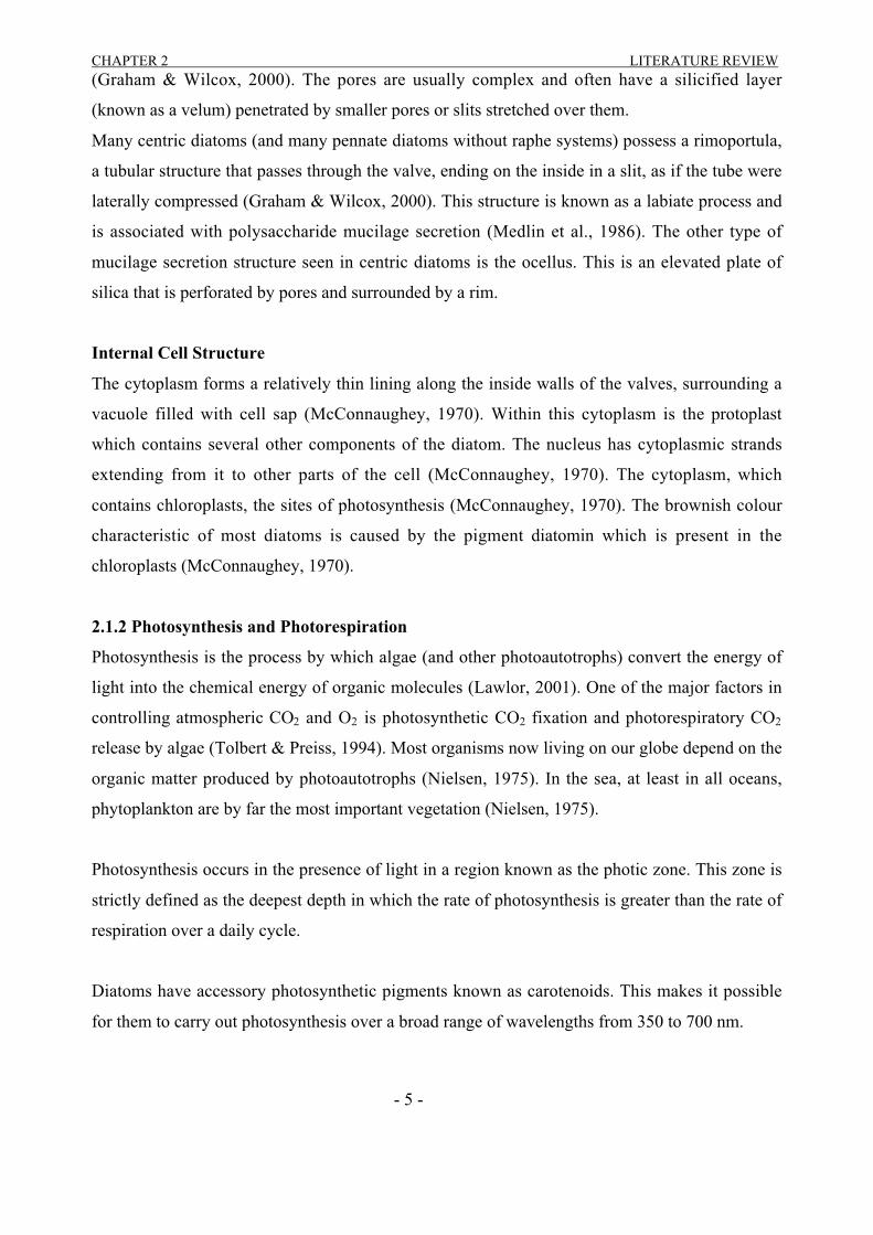
Diatoms use ribulose biphosphate carboxylase/oxygenase, or Ribisco for photosynthetic carbon
metabolism (Tolbert & Preiss, 1994). The carboxylase reaction initiates gross CO2 fixation by the
C3 reductive photosynthetic carbon cycle, and the oxygenase reaction initiates the C2 oxidative
photosynthetic carbon cycle for energy and CO2 loss by respiration (Figure 2.1.5) (Tolbert &
Preiss, 1994). These reactions can coexist, but it has been hypothesised that they depend on the
concentrations of CO2 and O2 (see Tolbert & Preiss, 1994, Graham & Wilcox, 2000).
Figure 2.1.4: Illustration of simultaneous gross photosynthetic CO2 fixation by the C3 cycle and
photorespiration by the C2 cycle (Tolbert & Preiss, 1994).
2.1.3 Reproduction
Diatoms reproduce vegetatively by binary fission, with two new individuals formed within the
parent cell frustule (Tomas, 1996). Each daughter cell receives one parent cell theca as epitheca,
and the cell division is terminated by the formation of a new hypotheca for each of the daughter
cells (Tomas, 1996). This type of division, with the formation of new siliceous components
inside the parent cell, leads to size reduction of the offspring (Tomas, 1996).
All diatoms are diploid, with meiosis at the end of the gametogenesis (Tomas, 1996). The zygote
develops into an auxospore (Tomas, 1996). In the centric diatoms, sexual reproduction is by
oogamy with flagellated male gametes, while most pennate diatoms are morphologically

CHAPTER 2 LITERATURE REVIEW
- 7 -
isogamous and lack a flagellated stage (Tomas, 1996). Relatively little is known regarding the
environmental cues that induce diatom sexual reproduction (Graham & Wilcox, 2000).
2.1.4 Diatom Spores and Resting Cells
Spores and resting cells allow diatoms to survive periods that are not suitable for growth, and
then germinate when conditions are suitable (Graham and Wilcox, 2000). Unsuitable conditions
for growth include periods of nutrient limitation. Both resting cells and spores are
characteristically rich in storage materials that supply the metabolic needs for germination
(Graham & Wilcox, 2000). Resting cells remain morphologically similar to vegetative cells,
whereas the frustules of spores become very thick and exhibit less elaborate ornamentation than
vegetative cells. Spores are believed to be capable of surviving for decades in benthic sediments.
The spores of marine diatoms often occur in mucoid aggregations (marine snow), and are
important in transporting organic carbon and silica to the sediments (Graham and Wilcox, 2000).
2.2 The Biological Pump and the Global Carbon Cycle
The increasing levels of atmospheric CO2 are of global concern to many research disciplines from
geology and ecology to the social sciences (Tolbert & Preiss, 1994). A major factor in controlling
atmospheric CO2 and O2 includes photosynthetic CO2 fixation and photorespiratory CO2 release
by algae (Tolbert & Preiss, 1994). This process of removal of free CO2 from the atmosphere and
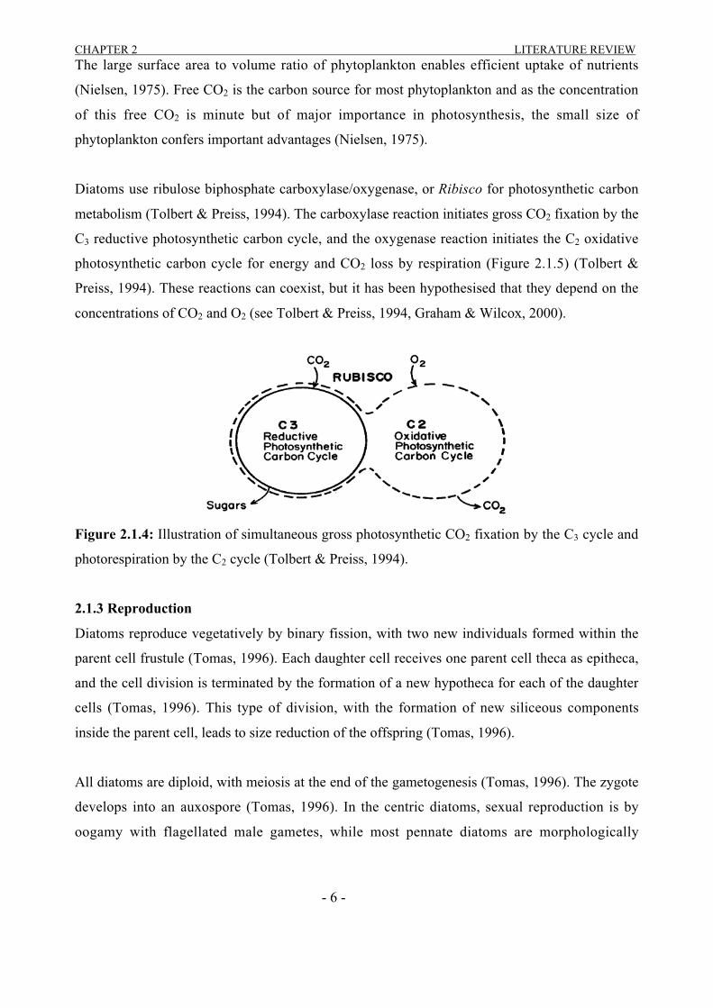
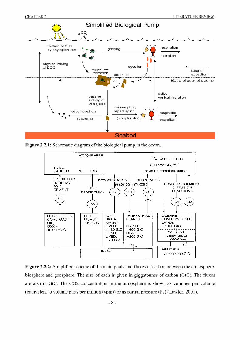
the ocean is commonly called the ‘biological pump’ (Figure 2.2.1). Second only to water vapour
in its importance as a heat trapping or ‘greenhouse’ gas, CO2 in the atmosphere is largely
maintained by exchanges with the much larger oceanic reservoir (Figure 2.2.2) (Norse, 1993,
Tolbert & Preiss, 2000, Lawlor, 2001).
CHAPTER 2 LITERATURE REVIEW
- 8 -
Figure 2.2.1: Schematic diagram of the biological pump in the ocean.
Figure 2.2.2: Simplified scheme of the main pools and fluxes of carbon between the atmosphere,
biosphere and geosphere. The size of each is given in giggatonnes of carbon (GtC). The fluxes
are also in GtC. The CO2 concentration in the atmosphere is shown as volumes per volume
(equivalent to volume parts per million (vpm)) or as partial pressure (Pa) (Lawlor, 2001).
CHAPTER 2 LITERATURE REVIEW
- 9 -
The surface waters of the world’s oceans contain less dissolved carbon than deep waters. This
vertical gradient is produced by phytoplankton in the photic zone (Norse, 1993), which take
dissolved carbon out of solution by photosynthesis (Norse, 1993, Lawlor, 2001). As a result of
several different factors (Section 2.3.2) the organic tissue of these diatoms sinks into deeper
waters or to the ocean floor, where it decomposes (Norse, 1993). The process of photosynthesis
followed by photoautotrophic sinking therefore pumps carbon from the surface to the deep ocean.
The total flow of fixed carbon downward from the surface waters of the global ocean is still
poorly known (Norse, 1993). The global carbon cycle is a good representation of the significance
of this ‘biological pump’ (Figure 2.2.2). Some of the most productive regions of the sea, where
the pump is working ‘hardest’, include the upwelling areas of continental shelves and slopes, and
the upwelling areas in the open ocean associated with wind driven divergences (Norse, 1993).
Although the oceans’ primary producers are very unlikely to die en masse, the Greenhouse Ocean
of the future is likely to be less productive than today’s, just as today’s ocean is known to be less
productive than the ocean during the glacial periods (Norse, 1993).
2.3 Phytoplankton Sinking Rate
As has been previously discussed the vertical flux of particulate carbon in the ocean is an
important parameter in the global carbon cycle and of potential significance to long-term changes
in atmospheric CO2 (e.g. Tolbert & Preiss, 1994).
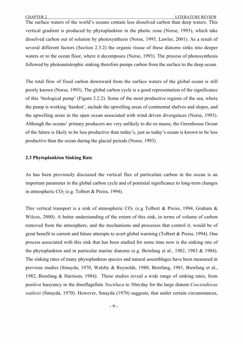
This vertical transport is a sink of atmospheric CO2 (e.g Tolbert & Preiss, 1994, Graham &
Wilcox, 2000). A better understanding of the extent of this sink, in terms of volume of carbon
removed from the atmosphere, and the mechanisms and processes that control it, would be of
great benefit to current and future attempts to avert global warming (Tolbert & Preiss, 1994). One
process associated with this sink that has been studied for some time now is the sinking rate of
the phytoplankton and in particular marine diatoms (e.g. Beinfang et al., 1982, 1983 & 1984).
The sinking rates of many phytoplankton species and natural assemblages have been measured in
previous studies (Smayda, 1970, Walsby & Reynolds, 1980, Beinfang, 1981, Bienfang et al.,
1982, Bienfang & Harrison, 1984). These studies reveal a wide range of sinking rates, from
positive buoyancy in the dinoflagellate Noctiluca to 30m/day for the large diatom Coscioidiscus
wailesii (Smayda, 1970). However, Smayda (1970) suggests, that under certain circumstances,

CHAPTER 2 LITERATURE REVIEW
- 10 -
much higher sinking rates are possible. The study of the sinking rates of different species of
phytoplankton in situ and in laboratory experiments, has resulted in more precise estimates of the
effectiveness of this carbon sink and the factors that control it.
The sinking velocity of a falling sphere was originally described by Stokes’ Law and is
applicable for Reynolds numbers less than one (John & Habermann, 1980). The Reynolds
number is the ratio of inertial forces to viscous forces (Streeter, 1971), and is described by the
equation:
µρ Udw=Re Equation 2.3.1
Stokes’ Law defines the terminal sinking velocity of a sphere through a fluid that is otherwise at
rest (Streeter, 1971). Stokes’ Law is described by the following equation:
µρρ
18)(2 gwpd
sw−
= Equation 2.3.2
Since phytoplankton are living and are often irregularly shaped , relative to a sphere, Hutchinson
(1967) modified Stokes’ Law to adjust sinking rates for the proportionality or shape factor of
nonspherical phytoplankton cells (Jassby, 1975). This modified form of Stokes’ law is:
µφ
ρρ
18
)(2 gwpdsw
−= Equation 2.3.3
Where:
ws is the sinking velocity in m s-1.
g is the gravitational acceleration of the earth (9.8 m s-1).
rs is the radius (m) of a sphere of volume equivalent to that of the algal cell.
ρ' is the density of the algal cell (kg m-3).
ρ is the density of the fluid medium (kg m-3).
µ is the viscosity of water (kg m-1 s-1).

CHAPTER 2 LITERATURE REVIEW
- 11 -
φ stands for the proportionality or shape factor and is dimensionless.
Phytoplankton that sink rapidly require more rapid vertical mixing to remain in the water column
than do cells that sink slowly (Graham & Wilcox, 2000). Phytoplankton have a number of
adaptations to reduce sinking rates (Graham & Wilcox, 2000):
• Small cell size, to allow for easier transport by currents.
• Larger diatoms have a reduced surface-to-volume ratio compared to smaller diatoms. This
means that they have proportionally less siliceous frustule material and are thus less dense
than small diatoms. Some marine diatoms such as species of Rhizosolenia and
Ethmodiscus can be positively buoyant (Graham & Wilcox, 2000).
2.3.1 Sinking Rate Measurement
Several methods had been employed in the past to measure the sinking rates of marine diatoms.
These methods can be broadly classified into two categories, depending on the initial distribution
of the sample in the settling chamber (Bienfang & Laws, 1977):
1. The discrete sample layer (DSL) method (e.g. Eppley et al., 1967).
2. The homogeneous sampling (HS) method (e.g. Titman 1975).
An analysis of technical and theoretical problems associated with the measurement of
phytoplankton sinking rates by these past methods indicates that they are both inaccurate and
imprecise (Bienfang & Laws, 1977).
More recently several new instruments have been developed that have improved the accuracy of
measuring phytoplankton sinking rates. These include the MARS instrument, the SETCOL
method, and the newly developed videography method. All of these methods have shown a
marked improvement in accuracy in comparison to the older methods.
The MARS instrument
The MARS instrument was developed as an improvement on the past methods described above.
The procedure involves detecting the transit time of radioactive (14C) labeled cells through a
settling column (Bienfang & Rothwell, 1978). A multichannel assembly for radio-plankton
sinking (MARS) instrument is used to detect the beta radiation emitted by the cells. The MARS
CHAPTER 2 LITERATURE REVIEW
- 12 -
instrument consists of eight inverted Geiger-Müller chamgers and a microprocessor linked to a
teletype.
The SETCOL method
Bienfang (1981) also developed the SETCOL method. The SETCOL method was developed
further by Waite et al (1992a) (Figure 2.3.1). The method developed by Waite et al (1992a)
utilises solely chlorophyll a concentrations instead of a combination of cell counts and
chlorophyll a concentrations, as was used by Beinfang (1981). This development measured final
concentrations of all SETCOL fractions (top, middle, and bottom fractions of the column) and
used these fractions to determine a mean sinking rate for a given culture (Waite et al., 1992a).
The equation used to determine sinking rate by this method is:
ws (m/day) = settle
cellbottombottombottom
Time
Length
aAveChlTotalVol
aAveChlVolaChlVol×
×
×−×
][
])][()][[( Equation 2.3.4
Where:
Volbottom is the volume drawn from the bottom outlet of a given SETCOL tube.
Chl[a]bottom is the chlorophyll a concentration of the volume drawn from the bottom outlet of a
given SETCOL column.
AveChl[a] is the average chlorophyll a concentration over the length of a given SETCOL tube.
This average is determined by summing the chlorophyll a concentrations for the top, middle and
bottom volumes drawn from a given tube and dividing this value by three.
TotalVol is the total volume drawn from a given SETCOL tube, i.e. the sum of the top, middle
and bottom volumes drawn.
Lengthcell is the length of he given SETCOL tube.
Timesettle is the time over which the SETCOL is left to settle before the three volumes are drawn
off.
The columns of the SETCOL instrument are filled with the sample, stirred and then left in the
dark for a given time to allow settling. After the settling time volumes are drawn off at the top
middle and bottom of each column. The volumes drawn off are then processed to determine

CHAPTER 2 LITERATURE REVIEW
- 13 -
chlorophyll a concentrations. The values obtained are then substituted into Equation 2.3.4 giving
a bulk sinking or ascent rate for the sample.
Figure 2.3.1: SETCOL instrument as developed by Waite et al (1997). Consisting of four
symmetric columns (1, 2, 3 & 4) immersed in a water bath, with outlets for the columns at the
top, middle and bottom.
Video Observation
This method is a new development that employs video images to determine the sinking rate and
size of phytoplankton. The method uses the same concept of non-disruptive observation of a
simulation of phytoplankton dynamics as used by Waite et al (1997).
The system used here is slightly different to that seen in the flocculation observation method
(Section 2.4.3). The camera still uses the same objective of 20x but due to the lower speeds of the
moving particles the shutter speed is reduced (Figure 2.3.2).
Light Source
Slit in Box Power Source
Microscope Objective
Culture Media
In Square column
Camera
JunctionBox
Monitor
In
VCRInOut
1 2 3 4
CHAPTER 2 LITERATURE REVIEW
- 14 -
Light Beam Stand
Figure 2.3.2: Plan view of setup of video monitoring of sinking rate.
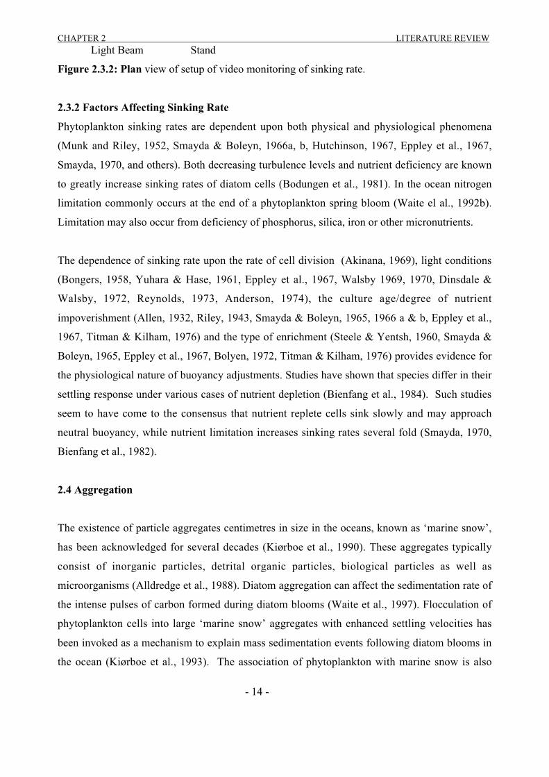
2.3.2 Factors Affecting Sinking Rate
Phytoplankton sinking rates are dependent upon both physical and physiological phenomena
(Munk and Riley, 1952, Smayda & Boleyn, 1966a, b, Hutchinson, 1967, Eppley et al., 1967,
Smayda, 1970, and others). Both decreasing turbulence levels and nutrient deficiency are known
to greatly increase sinking rates of diatom cells (Bodungen et al., 1981). In the ocean nitrogen
limitation commonly occurs at the end of a phytoplankton spring bloom (Waite el al., 1992b).
Limitation may also occur from deficiency of phosphorus, silica, iron or other micronutrients.
The dependence of sinking rate upon the rate of cell division (Akinana, 1969), light conditions
(Bongers, 1958, Yuhara & Hase, 1961, Eppley et al., 1967, Walsby 1969, 1970, Dinsdale &
Walsby, 1972, Reynolds, 1973, Anderson, 1974), the culture age/degree of nutrient
impoverishment (Allen, 1932, Riley, 1943, Smayda & Boleyn, 1965, 1966 a & b, Eppley et al.,
1967, Titman & Kilham, 1976) and the type of enrichment (Steele & Yentsh, 1960, Smayda &
Boleyn, 1965, Eppley et al., 1967, Bolyen, 1972, Titman & Kilham, 1976) provides evidence for
the physiological nature of buoyancy adjustments. Studies have shown that species differ in their
settling response under various cases of nutrient depletion (Bienfang et al., 1984). Such studies
seem to have come to the consensus that nutrient replete cells sink slowly and may approach
neutral buoyancy, while nutrient limitation increases sinking rates several fold (Smayda, 1970,
Bienfang et al., 1982).
2.4 Aggregation
The existence of particle aggregates centimetres in size in the oceans, known as ‘marine snow’,
has been acknowledged for several decades (Kiørboe et al., 1990). These aggregates typically
consist of inorganic particles, detrital organic particles, biological particles as well as
microorganisms (Alldredge et al., 1988). Diatom aggregation can affect the sedimentation rate of
the intense pulses of carbon formed during diatom blooms (Waite et al., 1997). Flocculation of
phytoplankton cells into large ‘marine snow’ aggregates with enhanced settling velocities has
been invoked as a mechanism to explain mass sedimentation events following diatom blooms in
the ocean (Kiørboe et al., 1993). The association of phytoplankton with marine snow is also

CHAPTER 2 LITERATURE REVIEW
- 15 -
considered to be a mechanism for their rapid removal from a nutrient depleted environment
(Smetacek, 1985).
This process can terminate a bloom before nutrients are fully depleted at the surface, and enhance
the ‘biological pump’ process. If the depths to which these aggregates sink are large, the
particulate carbon in such aggregates will not be returned to the atmosphere for long periods of
time, as shown by Tolbert and Preiss (1994). Aggregation also changes the availability of food to
grazers, especially those with size preferences for their prey as shown by (Rubenstein & Koel,
1977). Therefore, the dynamics of aggregates associated with marine diatoms are of major
importance to the fate of diatom carbon in coastal ecosystems (Waite et al., 1997) and to primary
productivity.
2.4.1 Causes of Aggregation: Observations
Aggregation has been monitored both in the laboratory and in the field. In the field aggregates are
commonly referred to as marine snow, which can consist of material other than a specific
phytoplankton species. Observations in the field and laboratory have led to the formulation of
several different hypotheses on the conditions required to cause such aggregation. The main
premise of these theories is that the rate of formation of these aggregates depends on the rate at
which single cells collide (Kiørboe et al., 1990).
2.4.2 Formation of Aggregates
The rate of formation of phytoplankton aggregates depends on the rate at which single cells
collide (Kiørboe et al., 1990). This process is considered to be mainly physically controlled, and
depends on the probability of adhesion upon collision (Kiørboe et al., 1990). This probability is
in turn dependent upon physio-chemical and biological properties of the cells (Kiørboe et al.,
1990). In nature these factors can occur as the result of different processes.
Diatom Blooms
Seasonally high nutrient concentrations often result in algal blooms with high biomass and
particle concentrations (Jackson et al., 1992). After such blooms flocs have been observed to
form (e.g. Alldredge et al., 1988). This is due to the resulting low nutrient levels at the bloom site
and the induction of resting states of the phytoplankton or mucilage excretion, which may cause
the cells to ‘stick’ together and sink out of the water column (Graham & Wilcox, 2000).
CHAPTER 2 LITERATURE REVIEW
- 16 -
Settling of Particles and other particulate matter
Aggregates have also been observed as they sink in the water column, increasing their average
size with increasing depth (Kranck & Milligan, 1988).
Nutritional state
Laboratory studies with algal cultures have shown that algal cells do indeed, have a finite chance
of sticking when they collide, and that this probability can change with nutritional state of the
algae and the algal species (Kiørboe et al., 1990).
2.4.3 Aggregation Quantification Methods
Several methods have been developed to determine the rate of aggregation of phytoplankton. Past
methods have been inaccurate in their ability to estimate ‘stickiness’ and aggregate size. New
methods, however, have shown increased accuracy of the measurement of cell stickiness and
aggregate size as a result of minimizing, and even preventing completely, the disturbance of
aggregates formed.
Past Methods
Typically, aggregation rates are quantified by observing phytoplankton cultures or field samples
in a cylindrical device known from the sanitary engineering literature as a flocculator (Waite et
al., 1997). This device generates a known laminar shear, and thus a known number of particle
collisions per unit time, for a given cell diameter and density. The collision and attachment of
cells in the flocculator results in changes in particle size distribution, which are quantified by
regularly sub sampling the spinning flocculator over short periods of time (< 1hour). From the
data acquired, one can quantify important aspects of aggregation such as the probability of
attachment between cells (stickiness, or α).
Disruption of aggregates has been observed to occur as a result of sub sampling and electronic
particle counting submitting suspensions to the high shear in the flocculator. This disruption is
difficult to predict because it is likely to be highly variable and species specific (Waite et al.,
1997). Cultures forming tight aggregates may be less susceptible to disruption than species
CHAPTER 2 LITERATURE REVIEW
- 17 -
forming loose aggregates. The accuracy of past aggregation measurements is potentially in doubt
(Waite et al. 1997).
Other methods of measuring stickiness have been attempted, but they involve either manual
quantification of individual aggregates or adhesion to artificial surfaces like glass or glass beads.
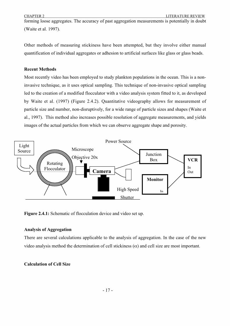
Recent Methods
Most recently video has been employed to study plankton populations in the ocean. This is a non-
invasive technique, as it uses optical sampling. This technique of non-invasive optical sampling
led to the creation of a modified flocculator with a video analysis system fitted to it, as developed
by Waite et al. (1997) (Figure 2.4.2). Quantitative videography allows for measurement of
particle size and number, non-disruptively, for a wide range of particle sizes and shapes (Waite et
al., 1997). This method also increases possible resolution of aggregate measurements, and yields
images of the actual particles from which we can observe aggregate shape and porosity.
Power Source
Microscope
Objective 20x
High Speed
Shutter
Figure 2.4.1: Schematic of flocculation device and video set up.
Analysis of Aggregation
There are several calculations applicable to the analysis of aggregation. In the case of the new
video analysis method the determination of cell stickiness (α) and cell size are most important.
Calculation of Cell Size
RotatingFlocculator Camera
JunctionBox
Monitor
In
VCR
InOut
LightSource

CHAPTER 2 LITERATURE REVIEW
- 18 -
The shape of cells has commonly been assumed to be spherical. This has been done in order to
gain a particle diameter measurement from a cross sectional area (Waite et al. 1997). The
particle diameter (d) can therefore be calculated from the following equation:
d = 2(X/π)1/2 Equation 2.4.1
Where X is the cross sectional area.
The cross sectional area of the cells is determined by video analysis.
Calculation of Stickiness
The video analysis of aggregation uses the method of determining stickiness developed by
Kiørboe et al (1990). This method depends on the increase in mean particle size over time as cells
collide and adhere to each other within the flocculator, according to the formula:
α = {m • π • exp(s2 / d2)}/(7.824 • V • S) Equation 2.4.2
Where α is stickiness, m is the slope of the natural log of particle diameter (µm) versus time (s),
s2 is the variance in the size distribution of the particles (µm) at t=0, d is the mean particle
diameter (µm), V is the volume fraction of particles at t=0 (ppm), and S in the mean shear rate (s-
1). This simplification is based on the assumption that any increase in mean particle size is caused
only by the collision and adhesion of single cells, forming doublets (Kiørboe et al., 1990).
Applicability of the Kiørboe et al (1990) Method
Waite et al (1997) tested the assumption of Kiørboe et al (1990) that any increase in mean
particle size is caused only by the collision and adhesion of single cells, forming doublets using
the video method they developed and two simple calculations. The distribution of nearest
neighbour distances (NNDs) within a culture allowed Waite et al (1997) to estimate the number
of cells packed in aggregates. NNDs were calculated by video analysis. They were then able to
compare the mean cell size in an experiment with one expected if all aggregates were doublets, as
assumed by the method of Kiørboe et al (1990).
CHAPTER 2 LITERATURE REVIEW
- 19 -
The method of Kiørboe et al (1990) was proven to be applicable in determining stickiness for the
initial stages of flocculation. Stickiness does not increase with increasing aggregate size, but only
with increased shear or increased physiological stressing of the diatom. Therefore, for a given
culture, the stickiness value determined from the early stages of flocculation is valid for all time.
CHAPTER 3 METHODOLOGY
- 19 -
3 METHODOLOGY
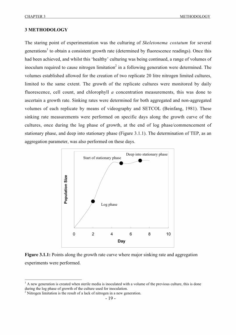
The staring point of experimentation was the culturing of Skeletonema costatum for several
generations1 to obtain a consistent growth rate (determined by fluorescence readings). Once this
had been achieved, and whilst this ‘healthy’ culturing was being continued, a range of volumes of
inoculum required to cause nitrogen limitation2 in a following generation were determined. The
volumes established allowed for the creation of two replicate 20 litre nitrogen limited cultures,
limited to the same extent. The growth of the replicate cultures were monitored by daily
fluorescence, cell count, and chlorophyll a concentration measurements, this was done to
ascertain a growth rate. Sinking rates were determined for both aggregated and non-aggregated
volumes of each replicate by means of videography and SETCOL (Beinfang, 1981). These
sinking rate measurements were performed on specific days along the growth curve of the
cultures, once during the log phase of growth, at the end of log phase/commencement of
stationary phase, and deep into stationary phase (Figure 3.1.1). The determination of TEP, as an
aggregation parameter, was also performed on these days.
0 2 4 6 8 10
Day
Po
pu
lati
on
Siz
e
Figure 3.1.1: Points along the growth rate curve where major sinking rate and aggregation
experiments were performed.
1 A new generation is created when sterile media is inoculated with a volume of the previous culture, this is doneduring the log phase of growth of the culture used for inoculation.2 Nitrogen limitation is the result of a lack of nitrogen in a new generation.
Log phase
Start of stationary phaseDeep into stationary phase
CHAPTER 3 METHODOLOGY
- 20 -
3.1 Culturing
The preparation of media, its constituents and its disinfection are of major importance so as to
maintain the validity of testing done on replicate cultures. The conditions under which a culture is
grown are of great importance to its health and consistency of growth, and extreme changes in
temperature and light conditions can have severe physiological effects on a culture (Bienfang et
al., 1982b, Bienfang et al., 1983). Several generations of Skeletonema costatum where grown
until consistency was achieved in the growth curves (determined by fluorescence readings) of
these cultures. The cultures were grown in G2 media (APPENDIX II). The culture generated for
aggregate sinking rate testing was limited in nitrogen so as to stress the diatoms. This stress was
expected to result an increase mucilage secretion by the cells, which in turn would produce
aggregates when a shear was introduced on the roller table (Section 3.2.1). Both aggregated and
non-aggregated volumes were analysed for individual (Video) and bulk (SETCOL) sinking rates.
3.1.1 Inoculation
Inoculation of all generations was done in a Laminar Flow Hood. The prepared media and the
previous cell generation were placed in the hood and treated with UV light for approximately five
minutes to kill off any introduced bacteria. Items coming into contact with one another were
either flamed (such as test tubes and conical flasks) or had previously been autoclaved and stored
to avoid contamination. The inoculation of new generations was done during the log phase of
growth to ensure the health of the Skeletonema costatum cultures.
3.1.2 Culturing Conditions
The conditions, such as light and temperature, under which the cultures were grown, were
controlled so that the growth of the cultures remained constant. Due to the different sizes of the
culture vessels the generations grown prior to the inoculation of the 20 litre culture vessels were
treated to slightly different conditions, with respect to light and temperature. The ‘healthy’
generations were growth in small 50 mL test tubes as well as three litre conical flasks. The light
and temperature conditions of the different culturing vessels could be assumed to be similar so
that the effect of the change in these conditions on the cultures would be negligible. The two
larger vessels were both stirred with magnetic stirrer bars, the 50 mL vessel, however, was not.
Comparison of the three liter and 50 mL cultures fluorescence levels was used to quantify any
discrepancies in growth rates due to turbulence, the effect of this was seen to be minimal.
CHAPTER 3 METHODOLOGY
- 21 -
Culture Media
The cultures were grown in a G2 media prepared as described in Appendix II. Prior to inoculation
of a new generation, the media was autoclaved to ensure disinfection. The source of phosphorus
was autoclaved separately and added prior to the inoculation of a new culture as it would have
precipitated if autoclaved with the other constituents. The addition of the phosphorus was done in
a Laminar Air Flow Hood with flaming of all contact surfaces. This was done to avoid infection
of cultures and the introduction of unwanted material.
Light Regime
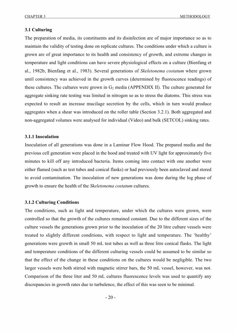
The light regime for culturing consisted of sixteen hours of daylight (culture lighting on)
followed by 8 hours of darkness (culture lighting off). This was achieved by the use of a timing
mechanism that turned the lights on and off when required (Figure 3.1.3). The lighting system for
culturing of the ‘healthy’ generations and for the replicate 20 liter carboys consisted of four
evenly spaced Thor 36 Watt white colour lights on racks either side of the vessels (Figure 3.1.4).
Figure 3.1.2: The timing device used to turn the lighting on and off.
CHAPTER 3 METHODOLOGY
- 22 -
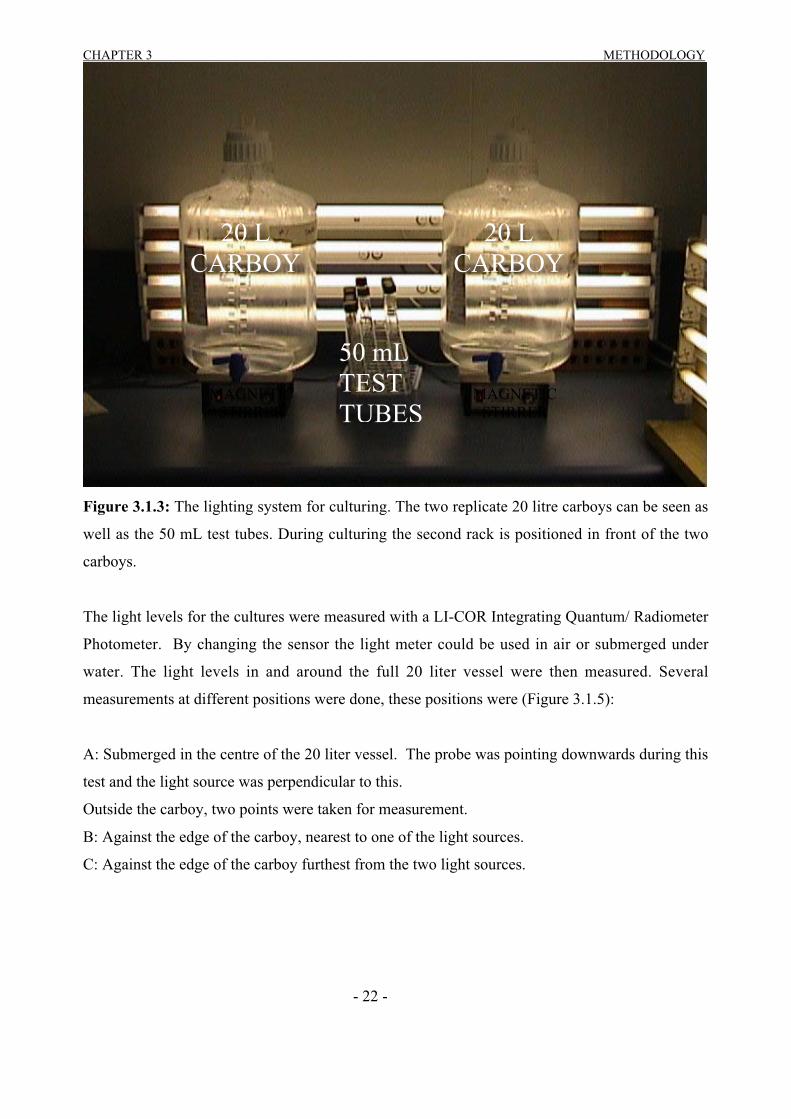
Figure 3.1.3: The lighting system for culturing. The two replicate 20 litre carboys can be seen as
well as the 50 mL test tubes. During culturing the second rack is positioned in front of the two
carboys.
The light levels for the cultures were measured with a LI-COR Integrating Quantum/ Radiometer
Photometer. By changing the sensor the light meter could be used in air or submerged under
water. The light levels in and around the full 20 liter vessel were then measured. Several
measurements at different positions were done, these positions were (Figure 3.1.5):
A: Submerged in the centre of the 20 liter vessel. The probe was pointing downwards during this
test and the light source was perpendicular to this.
Outside the carboy, two points were taken for measurement.
B: Against the edge of the carboy, nearest to one of the light sources.
C: Against the edge of the carboy furthest from the two light sources.
20 LCARBOY
20 LCARBOY
50 mLTESTTUBES
MAGNETICSTIRRER
MAGNETICSTIRRER

CHAPTER 3 METHODOLOGY
- 23 -
Figure 3.1.4: Positions of light meters for light level measurement.
The external light levels were then measured with a DSE Q-1400 Digital Lux Meter to determine
the accuracy of the LI-COR Photometer.
Table 3.1.1: The results of the LI-COR Photometer and the Digital Lux Meter. Using the
conversion rate of 1 klux = 12 µE.
Position LI-COR Lux Meter Converted Lux Meter
A 150µE NA NA
B 380µE 30 klux 360µE
C 200µE 17 klux 204µE
The light levels experienced by the cultures were assumed to be accurately measured by the LI-
COR Photometer.
The Effects of Changing Light Levels
Maintaining consistent light levels to a culture is one of the most important means of attaining
consistency in growth rate. The effects of changing the irradiance under which a culture grows
can severely affect the consistency of experiments performed on such cultures. This has been
LIGHTING RACK
LIGHTING RACK
A C
CHAPTER 3 METHODOLOGY
- 24 -
shown by Bienfang (1983), who proved that growth at low irradiance results in physiological
changes, which are manifested as changes in population buoyancy. Species within a culture adapt
to a given light regime if it is consistent, and will show consistent growth.
Reasons for Changing Light Levels
There are several reasons why the light levels within a culture may change. Firstly, as a culture
grows the biomass increases, and this increase may change the colour of the culture medium.
Light levels within the culture can also be affected by reflection and shading. It is therefore vital
to monitor the light levels within a large culture to ensure growth rate is not affected. Secondly,
coagulation can have an effect on light levels. Coagulation can be thought of as the process by
which small particles are converted into larger particles (Jackson et al., 1992). Aggregates cause
shading, which affects light levels received by individual diatoms and the aggregates themselves.
This effect would not be expected to occur in a 20 litre culture, due to the action of the magnetic
stirrer rod. Thirdly, the simulation of day and night is a common practice in culturing techniques.
Light levels within a culture room can be set by a timer that switches the lights on and off at
given times. This diurnal change in light levels, if kept constant, will not affect a culture because
of adaptation between light and dark. The temperature changes that occur as a result of this
change in light level could, however, have an effect on the growth of a culture (Bienfang et al.,
1982b).
Temperature Conditions
Due to the heating action of the light and the cooling action of the culture room temperature
changes in the cultures can be expected. The temperature conditions within the cultures were
monitored over a two-day period to determine any diurnal changes. To measure this the
StowAway® TidbiT® water temperature logger was used. The result of this monitoring showed
a diurnal temperature change of approximately 2oC. Due to the adaptive nature of Skeletonema
costatum (Mortian-Bertrand et al., 1988) with successive generations this effect was considered
negligible. These diurnal temperature changes are also a normal part of life in a water body, due
to the heating action of the sun.
Mixing Conditions
Mixing conditions within a culture solution can have considerable effect on the growth of the
culture. The two larger vessels were well mixed by magnetic stirrer rods. The result of stirring the

CHAPTER 3 METHODOLOGY
- 25 -
larger 20 litre vessel with a nitrogen limited culture could be the occurrence of unwanted
aggregates forming in the vessel (Figure 3.1.5). Simply having the stirrer speed low enough was
expected to avoid this effect.
Figure 3.1.5: Fluid motion in large 20L carboy.
3.1.3 Nitrogen Limitation
Stress was induced by nitrogen limitation, this was expected to cause the Skeletonema costatum
to exude a mucus or other exopolymeric material, and when a shear was induced to create
aggregates, which would then be observed for sinking rate and size.
Determination of Nitrogen Limitation Levels
To create a nitrogen limited generation the previous generation is added to G2 media, this new
media has not had the limiting substrate (nitrogen) added. The only supply of nitrogen is what
remains dissolved in the media of the previous generation. Several different volumes of a
previous generation were used to determine a range of different levels of nitrogen limitation
attainable. The raw fluorescence (fsu) of these cultures was monitored. A drop in the maximum
fluorescence attained by these limited cultures in comparison to the previous ‘healthy’
MAGNETIC
FLUID MOTION

CHAPTER 3 METHODOLOGY
- 26 -
generations value would indicate growth limitation of the culture, provided other conditions in
which the cultures are grown do not drastically change.
The culture to be used had been grown for several generations and had shown a consistent growth
rate of 1.3 day-1. Four different volumes of the ‘healthy’, non-limited, culture were added to
50mL of G2 medium that had no nitrogen added to it. This represented four different reduced
concentrations of nitrogen. The volumes added were 0.5mL, 1mL, 2mL, 4mL. The fluorescence
levels of all four cultures were then measured daily.
All four cultures showed an incremental level of growth limitation (Figure 3.1.6). Therefore the
volume of the previous generation to be added to the 20 liters of G2 media (without nitrogen)
could be determined depending on the level of limitation required.
1
10
100
1000
0 2 4
Day
Raw
Flu
ores
cenc
e (f
su)
0.5mL
1mL
2mL
4mL
Healthy
Figure 3.1.6: Growth curves of limited cultures, as measured by raw fluorescence.
Inoculation of Nitrogen Limited Culture
The two 20 litre carboys containing the G2 media (without nitrogen) were inoculated with 800mL
of ‘healthy’ culture. The ‘healthy’ culture was at the same stage of growth as in the nitrogen
limitation determination experiment. The volume of 800mL was intended to simulate the addition
of 2mL of ‘healthy’ culture to 50mL of G2 media (no nitrogen).
CHAPTER 3 METHODOLOGY
- 27 -
3.1.4 Replication and Inoculation of 20L cultures
The two 20 litre carboys were inoculated with 800mL each of the previous generation’s culture.
This was to achieve a form of replication so that results obtained from experiments could be
compared. Replication is the best means by which to validate results of such experiments.
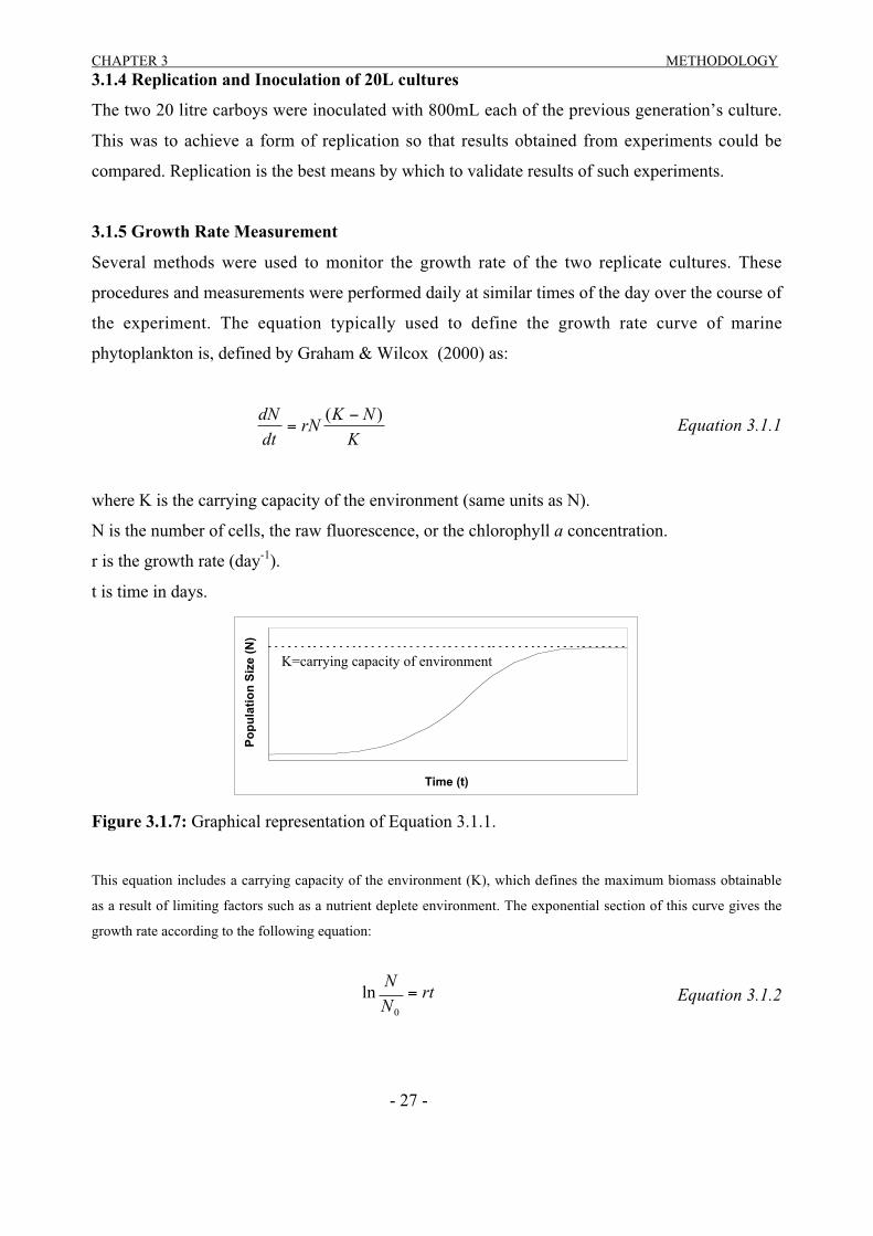
3.1.5 Growth Rate Measurement
Several methods were used to monitor the growth rate of the two replicate cultures. These
procedures and measurements were performed daily at similar times of the day over the course of
the experiment. The equation typically used to define the growth rate curve of marine
phytoplankton is, defined by Graham & Wilcox (2000) as:
K
NKrN
dt
dN )( −= Equation 3.1.1
where K is the carrying capacity of the environment (same units as N).
N is the number of cells, the raw fluorescence, or the chlorophyll a concentration.
r is the growth rate (day-1).
t is time in days.
Time (t)
Po
pu
lati
on
Siz
e (N
)
Figure 3.1.7: Graphical representation of Equation 3.1.1.
This equation includes a carrying capacity of the environment (K), which defines the maximum biomass obtainable
as a result of limiting factors such as a nutrient deplete environment. The exponential section of this curve gives the
growth rate according to the following equation:
rtN
N=
0
ln Equation 3.1.2
K=carrying capacity of environment
CHAPTER 3 METHODOLOGY
- 28 -
The variables are the same as those in Equation 3.1.1 except No is the number of cells, the raw
fluorescence, or the chlorophyll a concentration at the start of the logarithmic section of the
curve.
Coulter Counter Cell Count
The coulter counter gives an accurate measurement of the distribution of individual cell sizes.
Other outputs from this device are mean cell size, standard deviation of size and median
population statistics. The aperture used to measure the cultures was 200µm. Three size ranges
were used every time the test was run in order to ensure that all particles were counted, or to
determine if the population cell size distribution was changing. The size ranges used were 5 to
15µm, 4 to 12µm, and 2 to 6µm.
Fluorescence
The raw fluorescence (fsu) was measured with a Turner Designs TD-700 Fluorometer on a daily
basis over the course of the experiment for both replicates. This was to certify the results of the
other growth rate monitoring methods.
Chlorophyll a Concentration
50mL of each replicate culture was filtered through with a Whatman Glass Microfibre Filter
(GF/C) daily. The filters were then wrapped in foil and frozen for subsequent processing to
determine the chlorophyll a concentration by the method described in Appendix III.
3.2 Aggregation
Volumes of both replicates were aggregated on a roller table for approximately 120 minutes at 6
revolutions per minute. The aggregate volumes formed were tested for sinking rates using the
SETCOL and video methods. TEP measurements were taken as a measure of the amout of
exoplolymeric material exuded by the Skeletonema costatum.
3.2.1 The Roller Table
2 litre SCHOTT bottles were placed on the roller table for approximately two hours at a time.
The roller table spun the bottles on their axes at 6 revolutions per minute so as to create a shear
within the fluid. This imposed shear was expected to cause the particles in solution to collide
with one another and form aggregates (Figure 3.1.8).
CHAPTER 3 METHODOLOGY
- 29 -
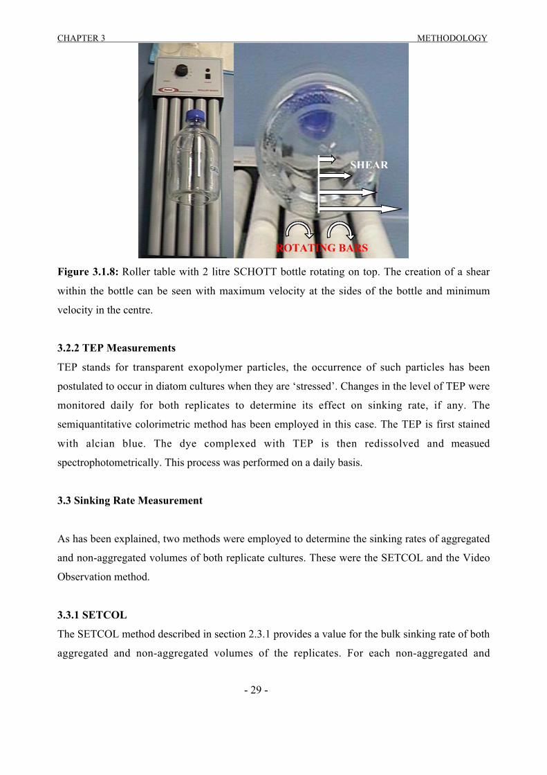
Figure 3.1.8: Roller table with 2 litre SCHOTT bottle rotating on top. The creation of a shear
within the bottle can be seen with maximum velocity at the sides of the bottle and minimum
velocity in the centre.
3.2.2 TEP Measurements
TEP stands for transparent exopolymer particles, the occurrence of such particles has been
postulated to occur in diatom cultures when they are ‘stressed’. Changes in the level of TEP were
monitored daily for both replicates to determine its effect on sinking rate, if any. The
semiquantitative colorimetric method has been employed in this case. The TEP is first stained
with alcian blue. The dye complexed with TEP is then redissolved and measued
spectrophotometrically. This process was performed on a daily basis.
3.3 Sinking Rate Measurement
As has been explained, two methods were employed to determine the sinking rates of aggregated
and non-aggregated volumes of both replicate cultures. These were the SETCOL and the Video
Observation method.
3.3.1 SETCOL
The SETCOL method described in section 2.3.1 provides a value for the bulk sinking rate of both
aggregated and non-aggregated volumes of the replicates. For each non-aggregated and
ROTATING BARS
SHEAR
CHAPTER 3 METHODOLOGY
- 30 -
aggregated volume, from each replicate, two SETCOL columns were used as a form of
replication. All SETCOL experimentation was performed in the dark in a cooled room.
3.3.2 Video Observation
This method was introduced in section 2.3.1. This method was used to determine the sinking
rates of both aggregated and non-aggregated volumes of the replicate 20L cultures.
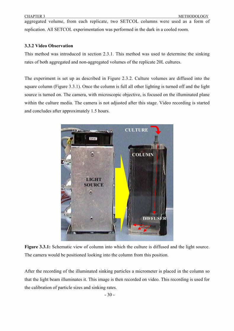
The experiment is set up as described in Figure 2.3.2. Culture volumes are diffused into the
square column (Figure 3.3.1). Once the column is full all other lighting is turned off and the light
source is turned on. The camera, with microscopic objective, is focused on the illuminated plane
within the culture media. The camera is not adjusted after this stage. Video recording is started
and concludes after approximately 1.5 hours.
Figure 3.3.1: Schematic view of column into which the culture is diffused and the light source.
The camera would be positioned looking into the column from this position.
After the recording of the illuminated sinking particles a micrometer is placed in the column so
that the light beam illuminates it. This image is then recorded on video. This recording is used for
the calibration of particle sizes and sinking rates.
LIGHTSOURCE
COLUMN
CULTURE
DIFFUSER
CHAPTER 3 METHODOLOGY
- 31 -
Calibration
Before the sinking rate and size are determined a calibration factor must be determined. The
calibration factor defines the number of pixels separating ten lines of the micrometer. This value
is then used to determine particle sizes and sinking displacements. To determine this calibration
factor a frame of the recording of the micrometer is ‘grabbed’, this ‘grabbed’ image is saved as a
‘tif’ file. To read the image from the ‘tif’ file to a MATLAB image a MATLAB m-file (a
program file) is used (Appendix VI) (Figure 3.3.2). Once the image of the micrometer has been
generated in MATLAB the calibration m-file can be run (Appendix V). However, several
variables must be defined in MATLAB, first:
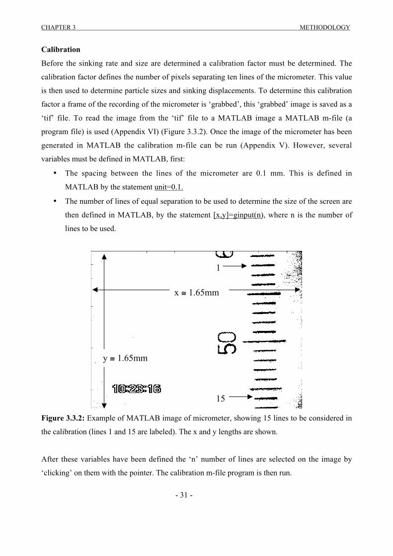
• The spacing between the lines of the micrometer are 0.1 mm. This is defined in
MATLAB by the statement unit=0.1.
• The number of lines of equal separation to be used to determine the size of the screen are
then defined in MATLAB, by the statement [x,y]=ginput(n), where n is the number of
lines to be used.
Figure 3.3.2: Example of MATLAB image of micrometer, showing 15 lines to be considered in
the calibration (lines 1 and 15 are labeled). The x and y lengths are shown.
After these variables have been defined the ‘n’ number of lines are selected on the image by
‘clicking’ on them with the pointer. The calibration m-file program is then run.
y ≅ 1.65mm
x ≅ 1.65mm
1
15

CHAPTER 3 METHODOLOGY
- 32 -
The output of this program is two x and two y values. The average of the two y values can be
assumed to define the number of pixels separating ten lines of the micrometer, i.e., 1mm. Two y
values are given due to the slight inaccuracy of visually selecting the exact positions of the lines
of the micrometer (Figure 3.3.2). The size of the image is considered to be square and so the
number of pixels per millimeter in the horizontal direction is considered the same as that in the
vertical direction (y value).
The calibration value is determined for each video due to any slight changes in the distance from
which the camera observes the particles, as this will have changed the field of view. The use of
this calibration factor is described below.
Determination of Particle Velocity
As with the micrometer footage, frame ‘grabs’ of the sinking chains and aggregates are taken, but
in this case a series of images are ‘grabbed’ at equal time intervals. Once these images are
grabbed the ‘trail’ image of a sinking particle can be created. This is done by converting the ‘tif’
images and then overlaying these images on one another, this can be done by the same m-file
program that converted the micrometer image (Figure 3.3.3). The m-file for converting the
images also makes the background black and the illuminated particles white.
Figure 3.3.3: An example of the image created when overlaying frames. The real image has been
cropped from the sides.
APPROXIMATELY 1.5mm
FRAME 1
FRAME 2
FRAME 3
FRAME 4
FRAME 5
FRAME 6
FRAME 7

CHAPTER 3 METHODOLOGY
- 33 -
The image of the trail of the particle can then be anlysed to determine the size (mm2) and the
sinking rate (mm s-1) of the given chain or aggregate. Both size and sinking rate are determined
by running the same MATLAB m-file program (APPENDIX VI). To determine sinking rate
several variables must be defined for the given trail in the MATLAB m-file program:
• The time step between ‘grabbed’ images must be defined (dt).
• The calibration factor must be defined (mmpx), as determined previously.
Once these variables have been adjusted for a given trail the number of particles in the trail must
be defined. In MATLAB define [x,y]=ginput(n), where n is twice the number of particles in the
trail. On the trail image the top left and bottom right of each particle in the trail are selected with
the pointer, down through the series of particles (Figure 3.3.4). The m-file program for sinking
velocity and size is then run and the velocity of the sinking particle is given (mm s-1).
The velocity of the particle is determined by the change of the displacement of the particle from
the top of the trail to the bottom over the given time period (dt) (Figure 3.3.4).
Figure 3.3.4: An example of the points used to determine sinking rate (green circles), and the
total displacement. The edges of the green box surrounding the aggregate are the limits of the
area within which the size of the aggregate is determined. This image total has been cropped.
TOP LEFT POINT SELECTED
BOTTOM RIGHT POINT SELECTED
TOTAL DISPLACEMENT
CHAPTER 3 METHODOLOGY
- 34 -
3.4 Particle Sizes
The determination of the individual particle sizes was performed on the video images obtained
with the use of a prepared MATLAB m-file program. Particle size distributions within the
aggregated and non-aggregated volumes were determined by the Counter Counter instrument.
3.4.1Coulter Counter
The Coulter Counter was used to determine the particle size distributions for both the SETCOL
and Video Sinking Rate methods. All three size range tests were performed to allow for possible
population size changes, as described in section 3.1.5.
3.4.2 MATLAB
The size estimation of specific Skeletonema costatum chains and aggregates was performed by
the same MATLAB m-file program and process as used to determine sinking rate. When
determining size the Central Limit Theorem is employed. There are slight differences in the size
of a particle in a trail due to the application of light intensity cut-offs. As a result of these slight
differences from particle to particle within a trail the range of sizes measured is assumed to be
part of a normal distribution.
Initially an area (x) for each particle in a trail is determined, based on the assumption that each
particle is defined by the area taken up by white pixels which have an intensity greater than that
of the background (black).
A distribution of the particle sizes due to the selection of multiple particles in a trail is then
analysed. This analysis is based on the central limit theorem3. Firstly a standard deviation (σ) of
the approximated particle sizes (x) is determined. Then a standard error (σx) based on the
standard deviation and the number of particles sampled (n) is determined, based on the
relationship nx σσ = .
3 The central limit theorem states that if a random sample of n observations is selected from a population, then whenn is sufficiently large, the sampling distribution of x will be approximately a normal distribution.

CHAPTER 3 METHODOLOGY
- 35 -
The z-statistic gives the distance between the estimated particle mean size and the actual particle
mean size, in units equal to the standard deviation:
x
xz
σµ−
= Equation 3.4.1
From this equation a range, or error, in estimating the actual size can be determined. Rearranging
equation 3.4.1 gives:
µσ ±×= xzx Equation 3.4.2
The plus (+) and minus signs (-) allow for estimates of the upper and lower limits, respectively,
of the particle size. The mean particle size is therefore determined as the average of these upper
and lower limits. The z-statistic is dependent on the number of particles used to define a trail,
generally the number of particles in the experiments was 5. Assuming a confidence interval of
95%, the relevant z-statistic is equal to 2.571.

CHAPTER 4 RESULTS
- 36 -
4 RESULTS
4.1 Growth rate
As has been described, several ‘healthy’ generations showing consistent growth rate needed to be
attained. This was to ensure the validity of any testing done. Only one method was used to
determine the growth rates of the generations prior to the inoculation of the 20 litre cultures, this
was raw fluorescence. The raw fluorescence curves for the three generations prior to the
inoculation of the 20 litre culture show a distinct consistency in slope from generation to
generation. A consistent growth rate of approximately 1.3 day-1 was achieved for the ‘healthy’
generations (Figure 4.1.1), this relates to a doubling of population size in half a day. The results
of the tests to monitor the growth of the major 20 litre replicate cultures show a distinct similarity
between the two, they are not, however, exactly the same. The growth rates during the
exponential phase of growth for the two replicate cultures were 0.71 day-1 and 0.64 day-1
respectively, using the raw fluorescence values obtained.
0
50
100
150
200
0 5 10 15
Time (Day)
Raw
Flu
ores
cenc
e (f
su)
Figure 4.1.1: The growth rate curves of the three previous ‘healthy’ generations of Skeletonema
Costatum prior to inoculation of the 20 L replicates.
4.1.1 Raw Fluorescence
The fluorescence levels of the replicates peaked on the same day (day 3) to approximately the
same levels (Table 4.1.1). The level of fluorescence dropped after this day (Table 4.1.1).
CHAPTER 4 RESULTS
- 37 -
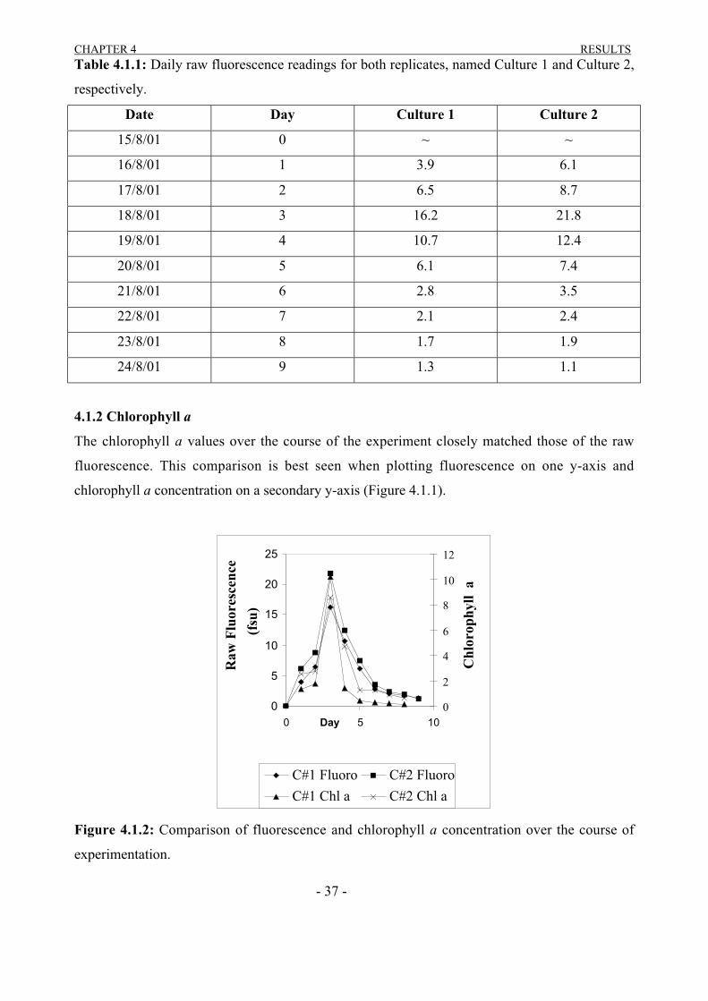
Table 4.1.1: Daily raw fluorescence readings for both replicates, named Culture 1 and Culture 2,
respectively.
Date Day Culture 1 Culture 2
15/8/01 0 ~ ~
16/8/01 1 3.9 6.1
17/8/01 2 6.5 8.7
18/8/01 3 16.2 21.8
19/8/01 4 10.7 12.4
20/8/01 5 6.1 7.4
21/8/01 6 2.8 3.5
22/8/01 7 2.1 2.4
23/8/01 8 1.7 1.9
24/8/01 9 1.3 1.1
4.1.2 Chlorophyll a
The chlorophyll a values over the course of the experiment closely matched those of the raw
fluorescence. This comparison is best seen when plotting fluorescence on one y-axis and
chlorophyll a concentration on a secondary y-axis (Figure 4.1.1).
0
5
10
15
20
25
0 5 10Day
Raw
Flu
ores
cenc
e
(fsu
)
0
2
4
6
8
10
12
Chl
orop
hyll
a
C#1 Fluoro C#2 Fluoro
C#1 Chl a C#2 Chl a
Figure 4.1.2: Comparison of fluorescence and chlorophyll a concentration over the course of
experimentation.

CHAPTER 4 RESULTS
- 38 -
4.1.3 Coulter Counter Cell Count
The Coulter Counter was the final means by which growth of the culture was measured. Once
again plotting raw fluorescence on one y-axis against cell count on a secondary y-axis shows the
similarity between the two over the first three days (Figure 4.1.2). The cell count, however, does
not seem to drop after the third day as chlorophyll a and raw fluorescence do, this could be due to
the fact that the dead cells that do not contribute to fluorescence and chlorophyll a, are still being
counted by the Coulter Counter.
0
5
10
15
20
25
0 2 4 6 8 10Day
Raw
Flu
ores
cenc
e (f
su)
0.0E+00
1.0E+05
2.0E+05
3.0E+05
4.0E+05
5.0E+05
6.0E+05
Cel
l Cou
nt
C#1 Fluoro C#2 Fluoro
C#1 Cell Count C#2 Cell Count
Figure 4.1.3: Comparison of fluorescence and cell counts over the course of experimentation.
4.2 Nitrogen Levels
The dissolved nitrogen levels were monitored over the course of the experiment. The filtrate of
the chlorophyll a measurements was frozen for this purpose and sent off for analysis. The levels
of dissolved nitrogen in both cultures was exactly the same for day zero and day one (Table
4.2.1). From day two onwards the level of dissolved nitrogen was practically non existent for
both replicates (approx. <7 µgL-1).
CHAPTER 4 RESULTS
- 39 -
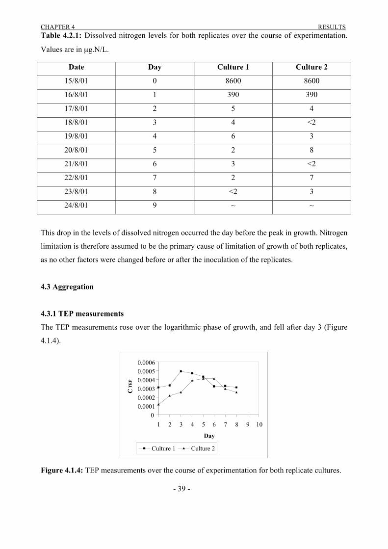
Table 4.2.1: Dissolved nitrogen levels for both replicates over the course of experimentation.
Values are in µg.N/L.
Date Day Culture 1 Culture 2
15/8/01 0 8600 8600
16/8/01 1 390 390
17/8/01 2 5 4
18/8/01 3 4 <2
19/8/01 4 6 3
20/8/01 5 2 8
21/8/01 6 3 <2
22/8/01 7 2 7
23/8/01 8 <2 3
24/8/01 9 ~ ~
This drop in the levels of dissolved nitrogen occurred the day before the peak in growth. Nitrogen
limitation is therefore assumed to be the primary cause of limitation of growth of both replicates,
as no other factors were changed before or after the inoculation of the replicates.
4.3 Aggregation
4.3.1 TEP measurements
The TEP measurements rose over the logarithmic phase of growth, and fell after day 3 (Figure
4.1.4).
00.00010.00020.00030.00040.00050.0006
1 2 3 4 5 6 7 8 9 10
Day
CT
EP
Culture 1 Culture 2
Figure 4.1.4: TEP measurements over the course of experimentation for both replicate cultures.

CHAPTER 4 RESULTS
- 40 -
4.4 SETCOL Size and Sinking Rates
The SETCOL and Video analysis methods were employed to determine the sinking rates of
aggregated and non-aggregated volumes of both replicates. As has been explained the results of
both methods differ in their final output as a result of their method of analysis. Each SETCOL
test produces one sinking rate value for the whole volume, whilst the Video analysis method
gives the sinking rates and sizes of individual particles or aggregates.
4.4.1 SETCOL Non-Aggregated Sinking Rates
The sinking rates as determined by the SETCOL method for the non-aggregated volumes of both
replicates show a significant increase in the mean sinking rate from day 2 two to day 5. Both
replicates show very low sinking rates on day 2 and for replicate culture 2 column 1 positive
buoyancy occurs. The mean sinking rates then drop slightly from day 5 to day 7 (Tables 4.4.1 &
4.4.2).
Table 4.4.1: Sinking rates for replicate culture 1 for both columns of the SETCOL.
Day Date Sinking rate for
column 1 (m day-1)
Sinking rate for
column 2 (m day-1)
Mean SR
(m day-1)
2 17/8/01 0.1340 0.1104 0.1222
5 20/8/01 0.3180 0.1511 0.2345
7 22/8/01 0.1632 0.2897 0.2265
Table 4.4.2: Sinking rates for replicate culture 2 for both columns of the SETCOL.
Day Date Sinking rate for
column 1 (m day-1)
Sinking rate for
column 2 (m day-1)
Mean SR
(m day-1)
2 17/8/01 -0.0378 0.1135 0.0378
5 20/8/01 0.4147 0.4128 0.4138
7 22/8/01 0.3139 0.3586 0.3362
4.4.2 SETCOL Aggregated Sinking Rates
Once again, as was seen in the non-aggregated results of the SETCOL there is a sharp increase in
the mean sinking rates from day 2 to day 5 for both culture replicates (Tables 4.4.3 and 4.4.4).
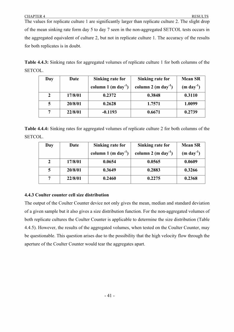
CHAPTER 4 RESULTS
- 41 -
The values for replicate culture 1 are significantly larger than replicate culture 2. The slight drop
of the mean sinking rate form day 5 to day 7 seen in the non-aggregated SETCOL tests occurs in
the aggregated equivalent of culture 2, but not in replicate culture 1. The accuracy of the results
for both replicates is in doubt.
Table 4.4.3: Sinking rates for aggregated volumes of replicate culture 1 for both columns of the
SETCOL.
Day Date Sinking rate for
column 1 (m day-1)
Sinking rate for
column 2 (m day-1)
Mean SR
(m day-1)
2 17/8/01 0.2372 0.3848 0.3110
5 20/8/01 0.2628 1.7571 1.0099
7 22/8/01 -0.1193 0.6671 0.2739
Table 4.4.4: Sinking rates for aggregated volumes of replicate culture 2 for both columns of the
SETCOL.
Day Date Sinking rate for
column 1 (m day-1)
Sinking rate for
column 2 (m day-1)
Mean SR
(m day-1)
2 17/8/01 0.0654 0.0565 0.0609
5 20/8/01 0.3649 0.2883 0.3266
7 22/8/01 0.2460 0.2275 0.2368
4.4.3 Coulter counter cell size distribution
The output of the Coulter Counter device not only gives the mean, median and standard deviation
of a given sample but it also gives a size distribution function. For the non-aggregated volumes of
both replicate cultures the Coulter Counter is applicable to determine the size distribution (Table
4.4.5). However, the results of the aggregated volumes, when tested on the Coulter Counter, may
be questionable. This question arises due to the possibility that the high velocity flow through the
aperture of the Coulter Counter would tear the aggregates apart.
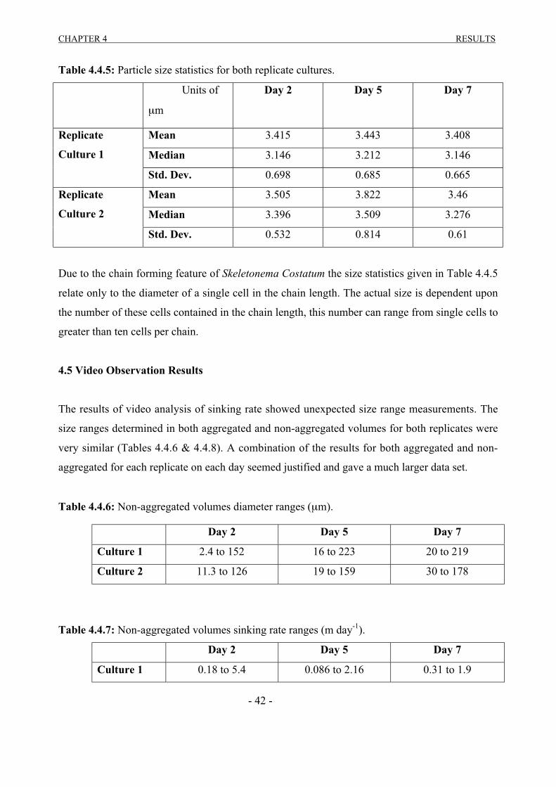
CHAPTER 4 RESULTS
- 42 -
Table 4.4.5: Particle size statistics for both replicate cultures.
Units of
µm
Day 2 Day 5 Day 7
Mean 3.415 3.443 3.408
Median 3.146 3.212 3.146
Replicate
Culture 1
Std. Dev. 0.698 0.685 0.665
Mean 3.505 3.822 3.46
Median 3.396 3.509 3.276
Replicate
Culture 2
Std. Dev. 0.532 0.814 0.61
Due to the chain forming feature of Skeletonema Costatum the size statistics given in Table 4.4.5
relate only to the diameter of a single cell in the chain length. The actual size is dependent upon
the number of these cells contained in the chain length, this number can range from single cells to
greater than ten cells per chain.
4.5 Video Observation Results
The results of video analysis of sinking rate showed unexpected size range measurements. The
size ranges determined in both aggregated and non-aggregated volumes for both replicates were
very similar (Tables 4.4.6 & 4.4.8). A combination of the results for both aggregated and non-
aggregated for each replicate on each day seemed justified and gave a much larger data set.
Table 4.4.6: Non-aggregated volumes diameter ranges (µm).
Day 2 Day 5 Day 7
Culture 1 2.4 to 152 16 to 223 20 to 219
Culture 2 11.3 to 126 19 to 159 30 to 178
Table 4.4.7: Non-aggregated volumes sinking rate ranges (m day-1).
Day 2 Day 5 Day 7
Culture 1 0.18 to 5.4 0.086 to 2.16 0.31 to 1.9

CHAPTER 4 RESULTS
- 43 -
Culture 2 0.07 to 2.45 0.06 to 1.37 0.17 to 0.82
Table 4.4.8: Aggregated volumes diameter ranges (µm).
Day 2 Day 5 Day 7
Culture 1 16 to 192 19 to 209 23 to 138
Culture 2 16 to 232 19 to 193 15 to 128
Table 4.4.9: Aggregated volumes sinking rate ranges (m day-1).
Day 2 Day 5 Day 7
Culture 1 0.06 to 4.23 0.14 to 2.1 0.27 to 1.66
Culture 2 0.095 to 4.99 0.1 to 1.18 0.19 to 1.3
The number of particles identified and analysed for size and sinking rate varied considerably
between tests, the smallest being 18 and the largest being 83 (Table 4.4.10).
Table 4.4.10: The number of particles identified in each test. Values in brackets represent total
particle numbers when combining the relative sets of data.
Day 2 Day 5 Day 7
Culture 1 Non-Aggregated 49 75 33
Culture 1 Aggregated 18 (67) 24 (99) 24 (57)
Culture 2 Non-Aggregated 42 83 65
Culture 2 Aggregated 58 (100) 74 (157) 31 (96)
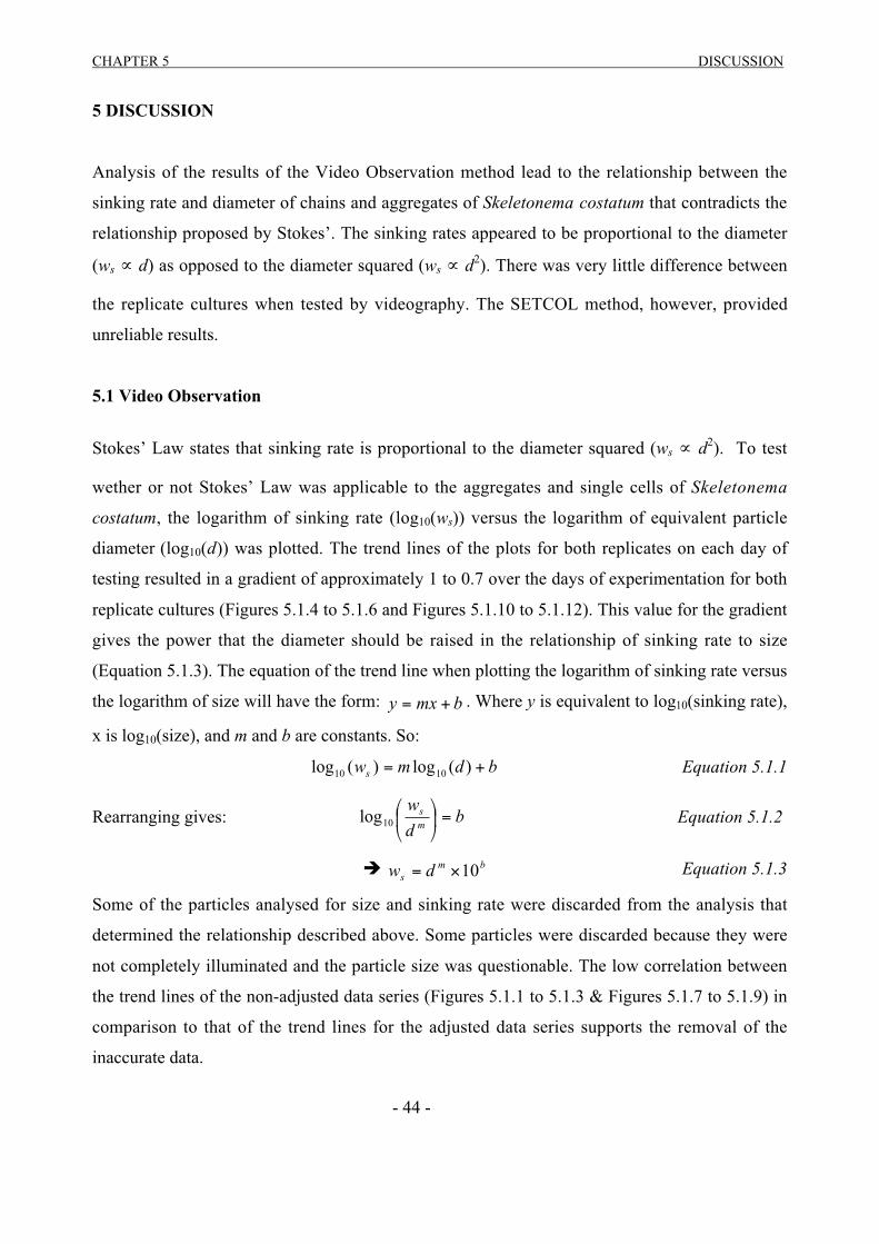
CHAPTER 5 DISCUSSION
- 44 -
5 DISCUSSION
Analysis of the results of the Video Observation method lead to the relationship between the
sinking rate and diameter of chains and aggregates of Skeletonema costatum that contradicts the
relationship proposed by Stokes’. The sinking rates appeared to be proportional to the diameter
(ws ∝ d) as opposed to the diameter squared (ws ∝ d2). There was very little difference between
the replicate cultures when tested by videography. The SETCOL method, however, provided
unreliable results.
5.1 Video Observation
Stokes’ Law states that sinking rate is proportional to the diameter squared (ws ∝ d2). To test
wether or not Stokes’ Law was applicable to the aggregates and single cells of Skeletonema
costatum, the logarithm of sinking rate (log10(ws)) versus the logarithm of equivalent particle
diameter (log10(d)) was plotted. The trend lines of the plots for both replicates on each day of
testing resulted in a gradient of approximately 1 to 0.7 over the days of experimentation for both
replicate cultures (Figures 5.1.4 to 5.1.6 and Figures 5.1.10 to 5.1.12). This value for the gradient
gives the power that the diameter should be raised in the relationship of sinking rate to size
(Equation 5.1.3). The equation of the trend line when plotting the logarithm of sinking rate versus
the logarithm of size will have the form: bmxy += . Where y is equivalent to log10(sinking rate),
x is log10(size), and m and b are constants. So:
bdmws += )(log)(log 1010 Equation 5.1.1
Rearranging gives: bd
wms =⎟⎠
⎞⎜⎝
⎛10log Equation 5.1.2
� bms dw 10×= Equation 5.1.3
Some of the particles analysed for size and sinking rate were discarded from the analysis that
determined the relationship described above. Some particles were discarded because they were
not completely illuminated and the particle size was questionable. The low correlation between
the trend lines of the non-adjusted data series (Figures 5.1.1 to 5.1.3 & Figures 5.1.7 to 5.1.9) in
comparison to that of the trend lines for the adjusted data series supports the removal of the
inaccurate data.

CHAPTER 5 DISCUSSION
- 44 -
y = 0.6403x + 2.6541
R2 = 0.4317
-1.5
-1
-0.5
0
0.5
1
-6 -5 -4 -3
log10(d)
log
10(w
s )
Figure 5.1.1: The non-adjusted data for
culture 1, day 2. 67 data points.
y = 0.9287x + 3.5396
R2 = 0.6796
-1.5
-1
-0.5
0
0.5
1
-5 -4.5 -4 -3.5 -3
log10(d)
log
10(w
s )
Figure 5.1.2: The non-adjusted data for
culture 1, day 5. 99 data points.
y = 0.4149x + 1.6152
R2 = 0.1749-1.5
-1
-0.5
0
0.5
1
-5 -4.5 -4 -3.5 -3
log10(d)
log 1
0(w
s )
Figure 5.1.3: The non-adjusted data for
culture 1, day 7. 57 data points.
y = 1.0471x + 4.379
R2 = 0.5319-1.5
-1
-0.5
0
0.5
1
-5 -4.5 -4 -3.5 -3
log10(d)
log 1
0(w
s )
Figure 5.1.4: The adjusted data for culture
1, day 2. 57 data points.
y = 0.9287x + 3.5396
R2 = 0.6796
-1.5
-1
-0.5
0
0.5
1
-5 -4.5 -4 -3.5 -3
log10(d)
log
10(w
s )
Figure 5.1.5: The adjusted data for culture
1, day 5. 99 data points.
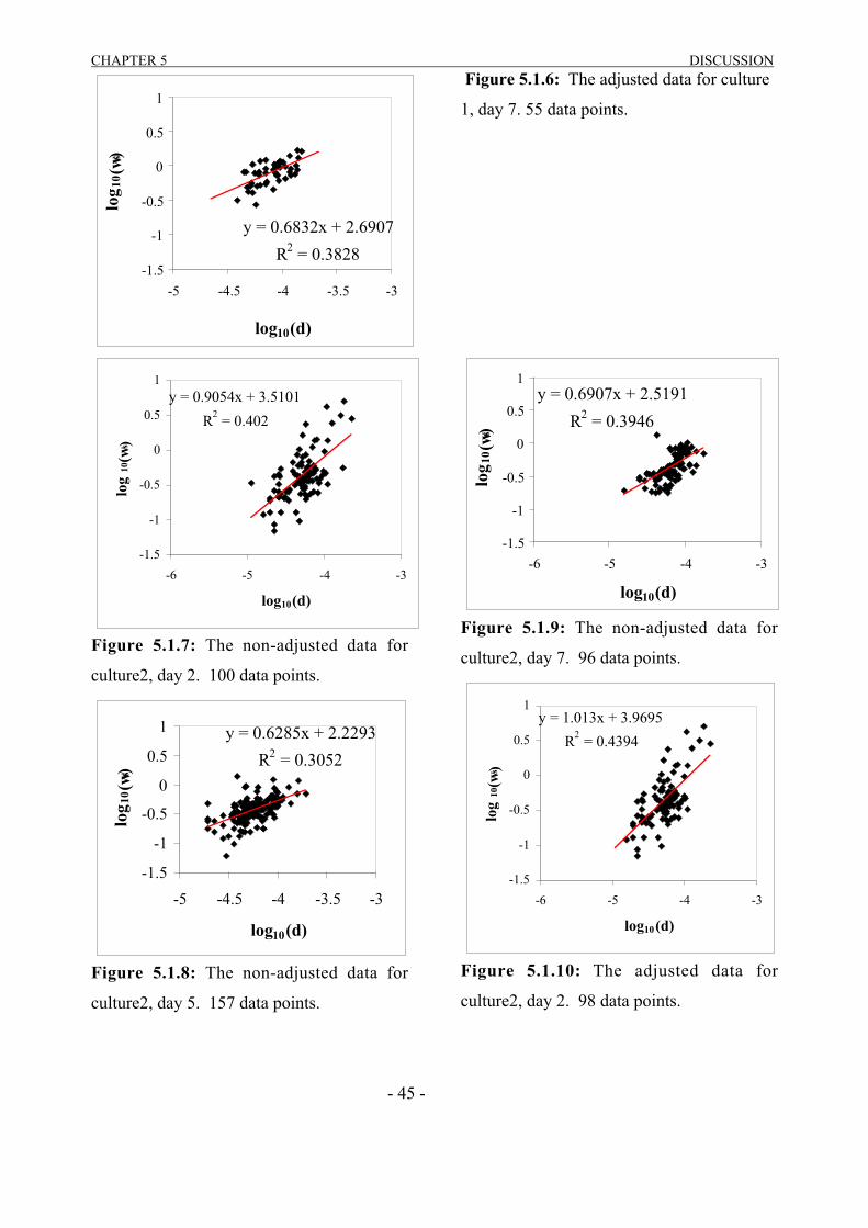
CHAPTER 5 DISCUSSION
- 45 -
y = 0.6832x + 2.6907
R2 = 0.3828-1.5
-1
-0.5
0
0.5
1
-5 -4.5 -4 -3.5 -3
log10(d)
log 1
0(w
s )
Figure 5.1.6: The adjusted data for culture
1, day 7. 55 data points.
y = 0.9054x + 3.5101
R2 = 0.402
-1.5
-1
-0.5
0
0.5
1
-6 -5 -4 -3
log10(d)
log
10(w
s )
Figure 5.1.7: The non-adjusted data for
culture2, day 2. 100 data points.
y = 0.6285x + 2.2293
R2 = 0.3052
-1.5
-1
-0.5
0
0.5
1
-5 -4.5 -4 -3.5 -3
log10(d)
log 1
0(w
s )
Figure 5.1.8: The non-adjusted data for
culture2, day 5. 157 data points.
y = 0.6907x + 2.5191
R2 = 0.3946
-1.5
-1
-0.5
0
0.5
1
-6 -5 -4 -3
log10(d)
log 1
0(w
s )
Figure 5.1.9: The non-adjusted data for
culture2, day 7. 96 data points.
y = 1.013x + 3.9695
R2 = 0.4394
-1.5
-1
-0.5
0
0.5
1
-6 -5 -4 -3
log10(d)
log
10(w
s )
Figure 5.1.10: The adjusted data for
culture2, day 2. 98 data points.
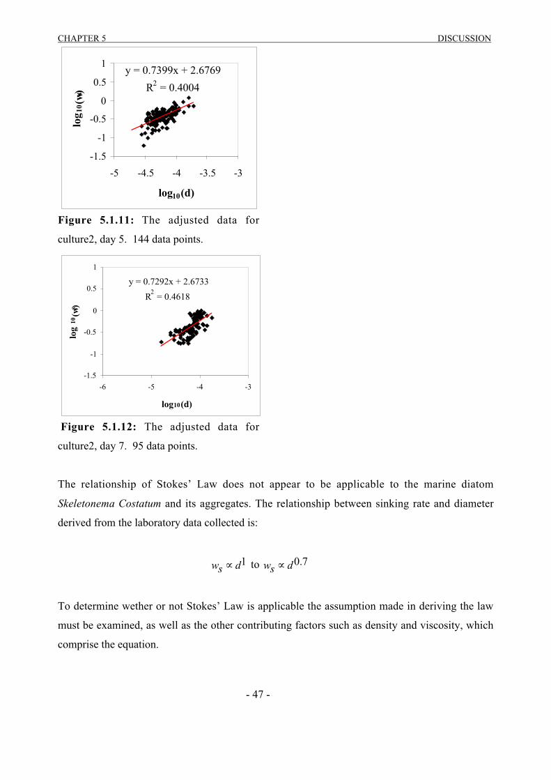
CHAPTER 5 DISCUSSION
- 47 -
y = 0.7399x + 2.6769
R2 = 0.4004
-1.5
-1
-0.5
0
0.5
1
-5 -4.5 -4 -3.5 -3
log10(d)
log 1
0(w
s )
Figure 5.1.11: The adjusted data for
culture2, day 5. 144 data points.
y = 0.7292x + 2.6733
R2 = 0.4618
-1.5
-1
-0.5
0
0.5
1
-6 -5 -4 -3
log10(d)
log
10(w
s )
Figure 5.1.12: The adjusted data for
culture2, day 7. 95 data points.
The relationship of Stokes’ Law does not appear to be applicable to the marine diatom
Skeletonema Costatum and its aggregates. The relationship between sinking rate and diameter
derived from the laboratory data collected is:
1dsw ∝ to 7.0dsw ∝
To determine wether or not Stokes’ Law is applicable the assumption made in deriving the law
must be examined, as well as the other contributing factors such as density and viscosity, which
comprise the equation.

CHAPTER 5 DISCUSSION
- 48 -
Stokes’ Law is considered applicable for low Reynolds number flow (Re<1). The maximum
Reynolds number achieved by the observed particles is:
Remax= 01445.010
))606024(5()10250(10003
6=
××÷×××=
××−
−
µρ sw wd Equation 5.1.4
The maximum Reynolds number is clearly less than 1. Therefore, with respect to Reynolds
number, Stokes’ Law holds true for the chains and aggregates of Skeletonema costatum.
The first assumption made when deriving Stokes’ Law is that the particle is travelling at its
terminal velocity. The largest time required to reach this terminal velocity would be for the
largest diameter particle (assuming a density of 1300 kg m-3), the longest time required is
therefore:
ondsd
T ppp sec109.3
1018
)10232(130018
33
262
−−
−
×=×
××==
µ
ρ Equation 5.1.5
The particles were observed toward the bottom of the column and because of this short time
required to reach terminal velocity, the chains and aggregates were considered to have reached
this velocity. Stokes’ Law still seems applicable, having considered the time taken to achieve
terminal velocity and the maximum size of the Reynolds number.
The equation for Stokes’ Law comprises a density factor as well as a viscosity factor. With
respect to the viscosity factor the media through which the Skeletonema costatum sink is assumed
to have a viscosity similar to that of water (10-3 kg m-1 s-1) and therefore is of no effect. The effect
of mucilage secretion as a means of changing density, measured by TEP (Section 4.3.1), has been
proposed as a means of reducing sinking rate. The effect of a mucilage ‘sheath’ in reducing the
overall density of the cell is mitigated by the consequent increase in the cell size. Sinking rate
would, however, be reduced if the mucilage was to comprise a larger volume than the cell alone.
From the video images the effect of this mucilage excretion in slowing the decent of the chains
and aggregates does not seem to be applicable. The solid edges of the chains and aggregates are

CHAPTER 5 DISCUSSION
- 49 -
visible and the amount of mucilage excreted would have to comprise a significant volume of the
size of the cells.
Another factor that could affect the density of the chains and aggregates of Skeletonema costatum
is the porosity of the aggregates and the hairlike protrusions that link the cells in chains. The
density of these porous aggregates would be significantly less than the density of a nonporous
particle of equivalent diameter. This density difference with respect to size may have an effect on
the density component of the Stokes’ Law equation, by simply reducing the density of the
aggregate relative to what the density would have been if the aggregate had been solid.
Finally, Hutchinson (1967), introduced the concept of form resistance (φ), this provides a factor
that determines the slowing effect that the shape of a chain or aggregate has on its sinking
velocity. Reynolds (1984) defines this form resistance as a ratio of predicted Stokes’ velocity (vs)
to actual velocity (ws).
swsv=φ Equation 5.1.7
Introducing this factor into Stokes’ Law gives:
µφ
ρρ
18
)(2 gdw wp
s
−= Equation 5.1.8
The value of vs can be defined as the gradient of Stokes’ relationship of log10(vs) versus the
log10(d), which is 2. The value of ws is therefore the value of the gradient of the plot of log10(ws)
versus the log10(d), which ranges from approximately 1 to 0.7 (Table 5.1.1).
Table 5.1.1: The form resistance values over the lifecycle of Skeletonema costatum.
Day 2 Day 5 Day 7
Culture 1 1.4 2.1 3.0
Culture 2 2.0 2.7 2.8
The application of this form resistance to the trendlines derived earlier would give the
relationship of sinking rate to diameter squared as proposed by Stokes’.
5.2 SETCOL
CHAPTER 5 DISCUSSION
- 50 -
The SETCOL method provides a bulk measurement of the sinking rate of both aggregated and
non-aggregated volumes. Several errors are associated with this form of determining bulk sinking
rate. These errors include changes in the diatom community during the course of
experimentation, breaking and forming of aggregates during stirring of media prior to
commencement of testing period, inaccurate particle size distribution determination and
inconsistency between replicate columns of the SETCOL. These errors are best seen in the results
of the aggregated volumes of the SETCOL. The non-aggregated volumes showed good
consistency, but the identification of aggregates by the Video Observation method show that
these tests were not performed on completely non-aggregated volumes. The results of the
SETCOL for these experiments can be considered inconclusive.

CHAPTER 6 CONCLUSIONS
- 50 -
6 CONCLUSIONS
The two methods used to determine sinking rates of the marine diatom Skeletonema costatum are
vastly different in technique and output.
Analysis of the results of the Video Observation method used to determine sinking rate showed
that there was a relationship between sinking rate and diameter (ws ∝ d) as opposed to Stokes’
relationship, that sinking rate is proportional to the diameter squared (ws ∝ d2). The conditions for
the application of Stokes’ Law to the chains and aggregates of Skeletonema coatatum were,
however, satisfied. As a result the concept of form resistance (φ) was added to the Stokes’ Law
equation, as proposed by Hutchinson (1967) and Reynolds (1984). This form resistance factor,
when included in Stokes’ Law adjusted the relationship between sinking rate and diameter
previously observed (ws ∝ d), to that of Stokes’ Law (ws ∝ d2). This form resistance is the result
of the non-spherical shape of the chains and aggregates of the marine diatom Skeletonema
costatum as well as a factor of porosity.
The SETCOL method is generally considered to give a good approximation of non-aggregated
settling rates of the marine diatom Skeletonema costatum. The SETCOL results for the non-
aggregated volumes are in question because of the observation of aggregates, in these volumes,
by the Video Observation method. These unwanted aggregates in the non-aggregated volumes
may be the result of the motion of the media within the 20 litre carboys.
The conclusions made about what has affected the sinking rate of the chains and aggregates of
the marine diatom Skeletonema costatum would be confirmed if different levels of nitrogen
limitation were tested as well as the testing of different forms of limitation.
REFERENCES
- 51 -
REFERENCES
Akinana D. K. (1969) Relative settling rate of dinoflagellata in relation to their rates of division.
Oceanology. 9: 248 – 250
Alldredge A.L., & Silver M.W. (1988a) Characteristics, dynamics and significance of marine
snow. Prog. Oceanogr. 20: 41 –82
Alldredge A. L., & Gotschalk C. C (1988b) Direct observations of the mass flocculation of
diatom blooms: Characteristics, settling velocities and the formation of diatom aggregates.
Deep Sea Res. 36: 159-171
Allen W. E. (1932) Problems of floatation and deposition of marine phytoplankton diatoms.
Trans. Am. Microsc. Soc. 51: 1 –7
Anderson L. W. J. (1974) Studies on the role of cellular lipids and inorganic ions in controlling
sinking rates of Ditylum brightwellii, a marine centric diatom. Ph. D. thesis, University of
California, Santa Barbara, 164pp.
Bienfang P. K., Laws E. (1977) Phytoplankton sinking rate determination: technical and
theoretical aspects, an improved methodology. J.exp. mar. Biol. Ecol. 30: 283 – 300
Bienfang P.K., & Rothwell G. N. (1978) MARS – A New instrument for measuring
phytoplankton sinking rate. Mar. Tech. Soc. Jour. 12: 13 – 17
Beinfang P. K. (1980) Phytoplankton sinking rates in oligotrophic waters off Hawaii, USA. Mar.
Biol. 61: 69 – 77
Bienfang P. K. (1981) SETCOL - A technologically simple and reliable method for measuring
phytoplankton sinking rates. Can. J. Fish. Aq. Sci. 38: 1289-1294
Bienfang P. K., Harrison P. J., & Quarmby L. M. (1982a) Sinking Rate Response to Depletion of
Nitrate, Phosphate and Silicate in Four Marine Diatoms. Marine Biology.
REFERENCES
- 52 -
Bienfang P. K., & Szyper J. P. (1982b) Effects of Temperature and Salinity on Sinking Rates of
the Centric Diatom Ditylum brightwelli. Biol. Oceanograph.
Bienfang P., Szyper J., & Laws E. (1983) Sinking rate and pigment responses to light limitation
of a marine diatom: implications to dynamics of chlorophyll maximum layers. Oceanol
Acta 6: 55-62
Bienfang P. K., Harrison P. J., & Quarmby L.M. (1984) Sinking-Rate response of natural
assemblages of temperate and subtropical phytoplankton to nutrient depletion. Marine
Biology.
Bodungen B. v. Bröckel K. v. Smetacek V. & Zeitzschel B. (1981) Growth and sedimentation of
the phytoplankton spring bloom in the Bornholm Sea (Baltic Sea). Unpublished.
Bolyen B. J. (1972) Studies on the suspension of the marine centric diatom Ditylum brightwellii
(West) Grunow. Int. Revue ges. Hydrobiol. 57: 585-597
Bongers L. H. J. (1958) Aspects of nitrogen assimilation by cultures of green algae. Meded. Van
de Landbouwhogeschool te Wageningen/Nederland. 56: 1 –52
Dinsdale M. T., & Walsby A. E. (1972) The interrelations of cell turgor pressure, gas vacuolation
and buoyancy in a blue-green alga. J. Exp. Bot. 23: 561-572
Downing D., & Clark J. (1989) Statistics the Easy Way, 2nd Ed. Barrons, New York.
Eppley R.W., Holmes R. W., & Strickland J. D. H. (1967) Sinking Rates of marine
phytoplankton measured with a fluorometer. Jour. Exp. Mar. Biol. Ecol. 1: 191 – 208
Graham L. E., & Wilcox L. W. (2000) Algae. Prentice-Hall, Inc.
Hutchinson G. E. (1967) A treatise on limnology, Vol. II. Introduction to lake biology and the
limnoplankton. 1115pp New York: J. Wiley

REFERENCES
- 53 -
Jackson G. A., & Lochmann S. E. (1992) Effect of coagulation on nutrient and light limitation of
an algal bloom. Limnol. Oceanogr. 37: 77-89
Jassby A. J. (1975) The ecological significance of sinking to planktonic bacteria. Can. J.
Microbiol. 21: 270-274
John J. E. A., & Haberman W. L. (1980) Introduction to Fluid Mechanics, 2nd Ed. Prentice-Hall,
Inc. New Jersey.
Johnson R. A., & Bhattacharyya G. K. (1992) Statistics, 2nd Ed. John Wiley & Sons, Inc. New
York.
Kiørboe T., Andersen K. P., & Dam H. G. (1990) Coagulation efficiency and aggregate formation
in marine phytoplankton. Mar. Biol. 107: 235-245
Kiørboe T., & Hansen L.S. (1993) Phytoplankton aggregate formation: observations of patterns
and mechanisms of cell sticking and the significance of exopolymeric material.
Kranck K., & Milligan T. (1988) Macroflocs from diatoms: In situ photography of particles in
Bedford Basin, Nova Scotia. Mar. Ecol. Prog. Ser. 44: 183-189
Lawlor D. W. (2001) Photosynthesis 3rd Edition. BIOS Scientific Publishers Ltd.
McClave J. T., & Deitrich F. H. II. (1992) A First Course in Statistics, 4th Ed. Macmillan, Inc.
New York.
McConnaughey B. H. (1970) Introduction to Marine Biology. The C. V. Mosby Company. Saint
Louis, USA.
Medlin L. K., Crawford R. M., & Anderson R. A. (1986) Histochemical and ultrastructural
evidence of the libate process in the movement of centric diatoms. British Phycological
Journal. 21: 297 – 301
REFERENCES
- 54 -
Mortian-Bertrand A., Descolas-Gros C., & Jupin H. (1988) Grwoth, photosynthesis and carbon
metabolism in the temperate marine diatom Skeletonema costatum adapted to temperature
and low photon-flux density. Mar. Biol. 100: 135-141
Munk H. W., & Riley G. A. (1952) Absorption of nutrients by aquatic plants. J. Mar. Res. 11:
215-240
Nielsen E. S. (1975). Elsevier Oceanography Series, 13: Marine Photosynthesis with special
emphasis on the ecological aspects. Elsevier Scientific Publishing Company. Amsterdam.
Norse E. A. (1993) Global marine biological diversity: A strategy for building conservation into
decision making. Island Press. Washington, USA.
Painter, T. J. (1983) Algal polysaccharides. In Aspinall, G.O. (ed.), The Polysaccharides.
Academic Press, London, Vol. 2, 196 – 285
Passow, U. & Alldredge A. L. (1995) A dye-binding assay for the spectrophotometric
measurement of transparent exopolymer particles (TEP). Limnol. Oceanogr. 40: 1326 –
1335
Reynolds C. S. (1973) Growth and buoyancy of Microcystis aeruginosa Kutz. Emend. Elkin in a
shallow eutrophic lake. Proc. R. Soc. B. 184: 29-50
Reynolds C. S. (1984) The Ecology of Freshwater Phytoplankton. University Press, Great
Britain.
Riley G. A. (1943) Physiological aspects of spring diatom flowering. Bull. Bingham Ocean Coll.
8: 1-53
Rubenstein D. I., & Koel M. A. R. (1977) The mechanisms of filter feeding: some theoretical
considerations. Am. Nat. 111: 981-994

REFERENCES
- 55 -
Smayda T.J., & Bolyen B. J. (1965) Experimental observations on the floatation of
marine diatoms. I. Talassiosira c.f. nana, Thalassiosira notula and Nitzschia
seriata. Limnol. Oceanogr. 10: 449-509
Smayda T.J., & Bolyen B. J. (1966a) Experimental observations on the floatation of
marine diatoms. II. Skeletonema costatum and Rhizosolenia setigera. Limnol.
Oceanogr. 11: 18-34
Smayda T.J., & Bolyen B. J. (1966b) Experimental observations on the floatation of marine
diatoms. III. Bacteriastrum byalinum and Chaetoceros landeri. Limnol. Oceanogr. 11: 35
43
Smetacek V.S. (1985) Role of sinking in diatom life history cycles: Ecology, evolutionary and
geological significance. Mar. Biol. 84: 239 – 251
Streeter V. L. (1971) Fluid Mechanics. McGraw-Hill, Inc. USA.
Titman D. (1975) A fluorometric technique for measuring sinking rates of fresh-water
phytoplankton. Limnol. Oceanogr. 20: 869 – 875
Titman D., & Kilham P. (1976) Sinking in freshwater phytoplankton: some ecological
implications of cell nutrient status and physical mixing processes. Limnol. Oceanogr. 21:
409-417
Tolbert N. E., & Preiss J. (1994) Regulation of atmospheric CO2 and O2 by photosynthetic
carbon metabolism. Oxford University Press, Oxford.
Tomas C.R. (1996) Identifying Marine Diatoms and Dinoflagellates. Academic Press, Inc.
California, USA.
Waite A. M., Thompson P. A., & Harrison P. J. (1992a) Does energy control the sinking rates of
marine diatoms? Limnol. Oceanogr. 37: 468-477

REFERENCES
- 56 -
Waite A. M., Bienfang P. K., & Harrison P. J. (1992b) Spring bloom sedimentation in a subarctic
ecosystem. I. Nutrient sensitivity. Mar. Biol. 112
Waite A. M., Bienfang P. K., & Harrison P. J. (1992c) Spring bloom sedimentation in a subarctic
ecosystem. II. Succession and sedimentation. Mar. Biol. 112
Waite A. M., Gallager S., & Dam H. G. (1997a) New measurements of phytoplankton
aggregation in a flocculator using videography and image analysis. Mar. Ecol. Prog. Ser.
155: 77-88
Waite A. M., Fischer A., Thompson P. A., Harrison P. J. (1997b) Sinking rate versus cell volume
relationships illuminate sinking rate control mechanisms in marine diatoms. Mar. Ecol.
Prog. Ser. 157: 97 - 108
Walsby A. E. (1969) The permeability of blue-green algal gas-vacuole membranes to gas. Proc.
R. Soc. B. 173: 235-255
Young D. F., Munson B. R., & Okiishi T. H. (1997) A Breif Introduction to Fluid Mechanics.
John Wiley & Sons, Inc. New York.
Yuhara T. Hase E. (1961) A brief note on the absorption of water by Chlorella cells during the
process of their lifecycle. J. gen. Appl. Microbiol., Tokyo. 7: 70-71
LI-COR, inc. Radiation Measurement Instruments Manual (1989) USA

APPENDIX I
- 57 -
Appendix I: CONSTITUENTS OF ARTIFICIAL SEAWATER
HYDRATED SALTS Grams/Litre Grams/15 Litres
MgCl2••••H2O 9.395 140.925
CaCl2••••2H2O 1.316 19.74
SrCl2••••6H2O 0.0214 0.321
ANHYDROUS SALTS Grams/Litre Grams/15 Litres
NaCl 20.758 311.37
Na2SO4 3.477 52.155
KCl 0.587 8.805
NaHCO3 0.17 2.55
KBr 0.0845 1.2675
H3BO3 0.0225 0.3375
NaF 0.0027 0.0405

APPENDIX II
- 58 -
Appendix II: CONSTITUENTS OF G2 MEDIUM (MAKES 3L)
Seawater 2250 mL
Deionised H2O 750 mL
Nitrate 3 mL
Vitamins 1.5 mL
PII metals 7.5 mL
Soil Extract 7.5 mL
Phosphate* 1.5 mL
*Note: Phosphate to be added in Laminar Air Hood.
APPENDIX III
- 59 -
Appendix III: PROTOCOL FOR THE EXTRACTION OF PHOTOSYNTHETICPIGMENTS
This method uses 90% acetone as the extraction solvent because of its relative low toxicity andits efficiency for most types of algae.
Chlorophyll a is the principle pigment used in the estimation of phytoplankton biomass.
This method uses the fluorometric readings to evaluate the concentration of chlorophyll a.
Sample Collection
Enough water should be collected to concentrate phytoplankton on at least 3 filters (WhatmanGF/F, Gelman A/E or equivalent) so that precision can be assessed. Filtration volume will dependon the particulate load of the water. 5L may be required in the open ocean, especially in the lowproductive areas like Perth Coastal Waters, whereas less than 1L can be sufficient for lakes orestuary waters. A sufficient volume has been filtered when a visible green or brown colour isvisible on the filter. Record the volume. Filtering should be performed in subdued light as soon aspossible after sampling due to the rapid degradation of chlorophyll a at increased temperaturesand light intensities. Fold the filter in half with the particulate matter on the inside, fold it againand place into a labelled 8mL snap cap tube (or aluminium foil) and place in a dark cool placeuntil they can be placed in a freezer or extracted straight away. Filters can be stored frozen for aslong as 3_ weeks without significant loss of chlorophyll a.
EXTRACTION BY GRINDING
Method
Take the samples from the freezer but keep them in a small esky on the bench, workspacelighting should be at a minimum. Remove filter from its tube with forceps and cut into smallpieces into the grinding tube. Push the filter to the bottom of the tube and add 4mL of 90 %acetone. Put the grinding tube into a beaker of crushed ice and grind the filter until it has beenconverted into a slurry. The ice should prevent overheating of the sample, which will causedegradation of the chlorophyll a. Pour the slurry into the 15mL glass centrifuge tube, use the 4mLpipette to rinse out the tube and the pestle and add the rinse to the centrifuge tube. Do this onemore time ensuring all the slurry has been removed from both the tube and the pestle. Place thebung on the tube and shake vigorously, place into the freezer. Rinse grinding tube and pestle withacetone and wipe with a tissue before proceeding onto the next filter. Shake each tube beforeputting them into the freezer to steep. The samples should be allowed to steep for a minimum of2 hours but not to exceed 24 hours.The tubes should be shaken at least once during this period.After steeping time, take samples from the freezer and shake again. Using a small (50mL) glassmanifold filter the extraction through a GF/F and pour the filtrate into a clean 13mm glass vial.Samples should be allowed to come to ambient temperature before analysis. Ensure that for eachrun a blank sample is also analysed.
Sample Analysis
Ensure the instrument you are using has warmed up for the minimum time required. Place thetube into the calibrated fluorometer (the instrument will need to be recalibrated if there has been a

APPENDIX III
- 60 -
3°C temperature fluctuation since the last calibration). Once the reading has stabilized record asthe Rb (before acid) result. Add 3 drops of 1N HCl to the tube, cap, shake and leave for 60seconds. Place in fluorometer and record reading Ra (after acid). Calculate the chlorophyll aconcentration from the following expression:
Chlorophyll a (mg/L) = (r/r-1)(Rb-Ra) v/V
r = the before-to-after acidification ratio of a pure chlorophyll a solution. Rb = fluorescence of a sample prior to acidification Ra = fluorescence of a sample after acidification v = volume (mL) of the extract V = volume of the filtered sample
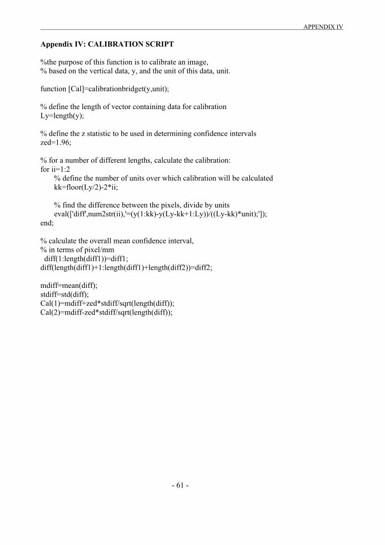
APPENDIX IV
- 61 -
Appendix IV: CALIBRATION SCRIPT
%the purpose of this function is to calibrate an image,% based on the vertical data, y, and the unit of this data, unit.
function [Cal]=calibrationbridget(y,unit);
% define the length of vector containing data for calibrationLy=length(y);
% define the z statistic to be used in determining confidence intervalszed=1.96;
% for a number of different lengths, calculate the calibration:for ii=1:2 % define the number of units over which calibration will be calculated kk=floor(Ly/2)-2*ii;
% find the difference between the pixels, divide by units eval(['diff',num2str(ii),'=(y(1:kk)-y(Ly-kk+1:Ly))/((Ly-kk)*unit);']);end;
% calculate the overall mean confidence interval,% in terms of pixel/mm diff(1:length(diff1))=diff1;diff(length(diff1)+1:length(diff1)+length(diff2))=diff2;
mdiff=mean(diff);stdiff=std(diff);Cal(1)=mdiff+zed*stdiff/sqrt(length(diff));Cal(2)=mdiff-zed*stdiff/sqrt(length(diff));
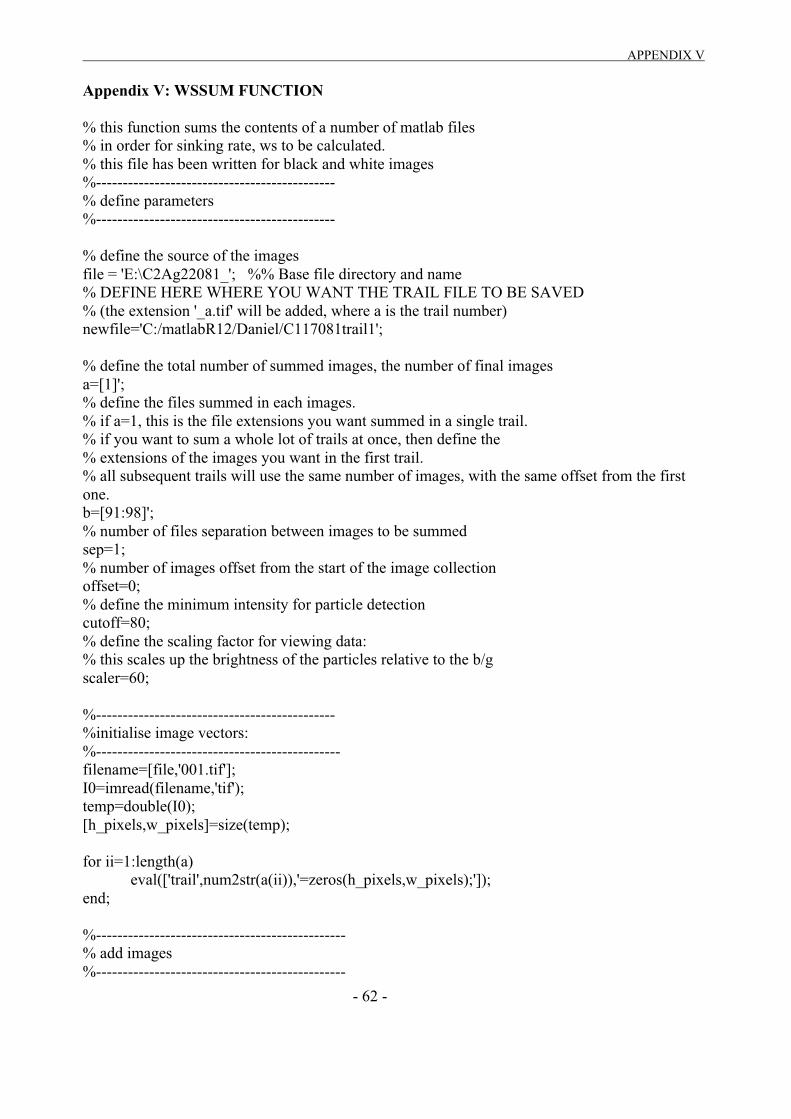
APPENDIX V
- 62 -
Appendix V: WSSUM FUNCTION
% this function sums the contents of a number of matlab files% in order for sinking rate, ws to be calculated.% this file has been written for black and white images%---------------------------------------------% define parameters%---------------------------------------------
% define the source of the imagesfile = 'E:\C2Ag22081_'; %% Base file directory and name% DEFINE HERE WHERE YOU WANT THE TRAIL FILE TO BE SAVED% (the extension '_a.tif' will be added, where a is the trail number)newfile='C:/matlabR12/Daniel/C117081trail1';
% define the total number of summed images, the number of final imagesa=[1]';% define the files summed in each images.% if a=1, this is the file extensions you want summed in a single trail.% if you want to sum a whole lot of trails at once, then define the% extensions of the images you want in the first trail.% all subsequent trails will use the same number of images, with the same offset from the firstone.b=[91:98]';% number of files separation between images to be summedsep=1;% number of images offset from the start of the image collectionoffset=0;% define the minimum intensity for particle detectioncutoff=80;% define the scaling factor for viewing data:% this scales up the brightness of the particles relative to the b/gscaler=60;
%---------------------------------------------%initialise image vectors:%----------------------------------------------filename=[file,'001.tif'];I0=imread(filename,'tif');temp=double(I0);[h_pixels,w_pixels]=size(temp);
for ii=1:length(a)eval(['trail',num2str(a(ii)),'=zeros(h_pixels,w_pixels);']);
end;
%-----------------------------------------------% add images%-----------------------------------------------

APPENDIX V
- 63 -
%% Now loop through each image, adding them:for ii=1:length(a)
for jj=1:round((length(b)-offset)/sep)filename=[file,sprintf('%03d',((a(ii)-1)*length(b)*sep+offset+b(1)+(jj-
1)*sep)),'.tif'];Im=imread(filename,'tif');%image(Im);temp=double(Im);%d=temp(upper_lim:lower_lim,left_lim:right_lim);
inc=or(temp>cutoff,0);eval(['trail',num2str(a(ii)),'=trail',num2str(a(ii)),'+inc;']);
clear Im;end;
trailtif=uint8(trail1); filenamenew=[newfile,'_',sprintf('%03d',a(ii)),'.tif']; eval(['trailtif=trail',num2str(a(ii)),';']); imwrite(trailtif,filenamenew,'tif');end;
%------------------------------------------------% display the image%------------------------------------------------for ii=1:length(a);
figure; eval(['trail=or(trail',num2str(a(ii)),'>0,0);']);
image(trail*scaler);
title(['file=',file,' a=',num2str(a'),' ,b=',num2str(b'),' ,sep=',num2str(sep),'*dt s']); colormap(gray);
clear trail;
end;
%------------------------------------------------% save the summed image in a separate .tif file

APPENDIX VI
- 64 -
Appendix VI: WSDATA FUNCTION
the purpose of this function is to read in pairs of data% which define the edges of each particle.% the vertical points are averaged to determine the mean particle positions, y% which are then used to calculate the velocity, v. % the data is also evaluated in pairs to define the mean area,% and upper and lower limits of area.% this data is then recorded in file filename
%---------------------------------------% clear unwanted variables%--------------------------------------clear dm se base top v atemp dtemp;
%---------------------------------------% define parameter values%---------------------------------------% define the filename where this data is stored% NB DO NOT INCLUDE .MAT EXTENSION HEREfilename='C:/matlabR12/dataC2Ag2208_13';
% define the z statisticzed=2.571;
% mm/pixel: in horizontal,x, and vertical,y, respectivelymmpx=1/333.4;mmpy=1/333.4;
% base timestep, sdt=10;
% time step for this calculationDt=dt*(length(y)/2-1);
%-------------------------------------%load data file%-------------------------------------% load data fileeval(['load ',filename,'.mat']);
%-------------------------------------% calculate velocity%-------------------------------------base=0.5*(y(length(y)-1)+y(length(y)));top=0.5*(y(1)+y(2));% determine toal displacement, convert to mm delta=abs((base-top)*mmpy);v=delta/Dt;

APPENDIX VI
- 65 -
%-------------------------------------% calculate area, equivalent diameter%------------------------------------- % round the pixel locations, to use as indices in calculating area:ry=round(y);rx=round(x);
% calculate the mean area, and confidence intervals for the area datafor ii=1:(length(ry)/2) atemp(ii)=sum(sum(trail(ry(2*ii-1):ry(2*ii),rx(2*ii-1):rx(2*ii))));end;
% convert area to mm2, and find std errora2temp=atemp*mmpx*mmpy;se=std(a2temp)/sqrt(length(a2temp));% define the mean equivalent diameter squareda2m(1,1)=mean(a2temp);% define upper and lower bounds on diametera2m(2,1)=a2m(1)-zed*se;a2m(3,1)=a2m(1)+zed*se;
%--------------------------------------% update data file%--------------------------------------
% update variablesa2(:,length(ws)+1)=a2mws(length(ws)+1)=vcounter(length(counter)+1)=length(y)/2% resave data fileeval(['save ',filename,'.mat a2 ws counter trail;']);