particle manipulation using electric field gradients in ...€¦ · appendix a: matlab code to...
TRANSCRIPT

Particle Manipulation Using Electric Field Gradients in Microdevices
Andrea Diane Rojas
Thesis submitted to the faculty of the Virginia Polytechnic Institute and State University
in partial fulfillment of the requirements for the degree of
Master of Science
In
Materials Science and Engineering
Rafael V. Davalos
Alex O. Aning
Abby R. Whittington
Eva M. Schmelz
February 1, 2012
Blacksburg, Virginia
Keywords: Electrokinetics, Bacterial Cellulose,
Breast Cancer, Contactless Dielectrophoresis
Copyright 2012

Particle Manipulation Using Electric Field Gradients in Microdevices
Andrea Diane Rojas
ABSTRACT
Electrokinetics is a family of effects that induces motion of a liquid or a particle within a liquid
in response to an external electric field. Using the intrinsic electrical properties of bacteria and of
breast cancer cells, electrokinetics can be used to manipulate these particles for two different
types of applications: tissue engineering and breast cancer detection. The first application studied
the effects of electric fields on bacteria cells as well as calcium ions to potentially create a
meniscus scaffold with hydroxyapatite ends for anchoring. In response to the electric field,
calcium ions were able to deposit locally and simultaneously with cellulose growth. Bacteria
cells were also studied to determine their response under an AC field. At low frequencies,
bacteria demonstrated controlled movement caused by electroosmosis and dielectrophoresis with
a net motion caused by a dielectrophoretic force.
In the second application, the separation capabilities of different stages of breast cancer cells
from the same cell line were tested using contactless dielectrophoretic (cDEP) devices. The
electric field gradients in cDEP devices were altered to optimize selectivity and to determine an
estimated membrane capacitance for each. From the results, the membrane capacitance of the
early to intermediate stages proved to be very similar; however, late stage breast cancer cells
have potential in being separated from early and intermediate stages.

iii
ACKNOWLEDGEMENTS
I would like to acknowledge all those in the Bioelectromechanical Systems Laboratory (BEMS)
for sharing their knowledge and wisdom with me. As well as those colleagues outside the BEMS
Laboratory who have taught me valuable theoretical and experimental knowledge that helped me
with my research. I would like to show my gratitude to Mike Sano for mentoring me throughout
the years as well as making sure I was safe around the electrical equipment in the laboratory. I
would like to thank Dr. Rafael Davalos for the opportunities he provided me in his laboratory as
well as for introducing me to this fascinating technology. Furthermore, I would like to thank Dr.
Alex Aning who guided me in the right direction of my life by encouraging me to pursue an
advanced degree. I am thankful to all of my friends who have made my time here enjoyable and
full of great memories.
Lastly, I would like to say thank you to my family especially my parents for showing their love
and support every step of the way. Without them, I would not be where I am today. I dedicate
this thesis to my wonderful parents, Fernando and Claudia Rojas.

iv
Table of Contents
Table of Contents ........................................................................................................................... iv
List of Figures ................................................................................................................................. v
List of Tables ................................................................................................................................ vii
Chapter 1. Introduction ................................................................................................................... 1
Chapter 2. Background & Significance .......................................................................................... 2
2.1 Directed Motion of Bacteria and Calcium Ions to Create a Meniscus .................................. 2
2.2 Separation of Breast Cancer Cells for Personalized Medicine ............................................. 5
Chapter 3. Electrokinetic Theory .................................................................................................. 10
3.1 Electrokinetics in a Uniform Electric Field......................................................................... 10
3.2 Electrokinetics in a Non-uniform Electric Field ................................................................. 11
3.3 Clausius-Mossotti (CM) Factor ........................................................................................... 14
Chapter 4. Methods and Materials ................................................................................................ 17
4. 1 Microdevice Fabrication .................................................................................................... 17
4. 2 Cell Culture Protocol .......................................................................................................... 19
Chapter 5. Bacterial Cellulose Studies.......................................................................................... 23
5.1 Experimental Procedures..................................................................................................... 23
5.2 Results and Discussion ........................................................................................................ 24
5.3 Future Work ........................................................................................................................ 30
Chapter 6. Separation of Breast Cancer by Stage ......................................................................... 32
6.1 Experimental Procedures..................................................................................................... 32
6.2 Results and Discussion ........................................................................................................ 34
6.3 Future Work ........................................................................................................................ 44
Chapter 7. Conclusions ................................................................................................................. 45
References ..................................................................................................................................... 46
Appendix A: MATLAB Code to Analyze Results from High Frequency cDEP Experiments .... 50
Appendix B: MATLAB Code to Analyze Results from Low Frequency cDEP Experiments ..... 55
Appendix C: MATLAB Code for Plotting the Clausius-Mossotti Curve..................................... 58

v
List of Figures
All figures by author unless otherwise cited
Figure 1. Bacterial cellulose (a) network of fibers viewed under SEM and (b) pellicle formed at
air/liquid interface ........................................................................................................................... 3
Figure 2. Bacterial cellulose coated with copper [20] .................................................................... 4
Figure 3. A meniscus made of circumferential fibers with radial fibers integrated within the
network ........................................................................................................................................... 4
Figure 4. Electric field turned on with flow from right to left showing cells being trapped on the
insulating posts. This was the cDEP device used in separating live and dead cells as well as
breast cancer cells by stage[58] ...................................................................................................... 8
Figure 5. Electroosmotic flow is more uniform across the width of the channel while pressure
driven flow is parabolic ................................................................................................................ 11
Figure 6. The net force on a dipole (a) and a polarized particle (b) ............................................. 12
Figure 7. Single shell model of a cell comprised of a cytoplasm core and membrane as an outer
shell with radii r1and r2 ................................................................................................................. 13
Figure 8. The Clausius-Mossotti curve of an early stage breast cancer cell modeled using the
single shell model ......................................................................................................................... 16
Figure 9. Sample polycarbonate stamp to create channels ........................................................... 17
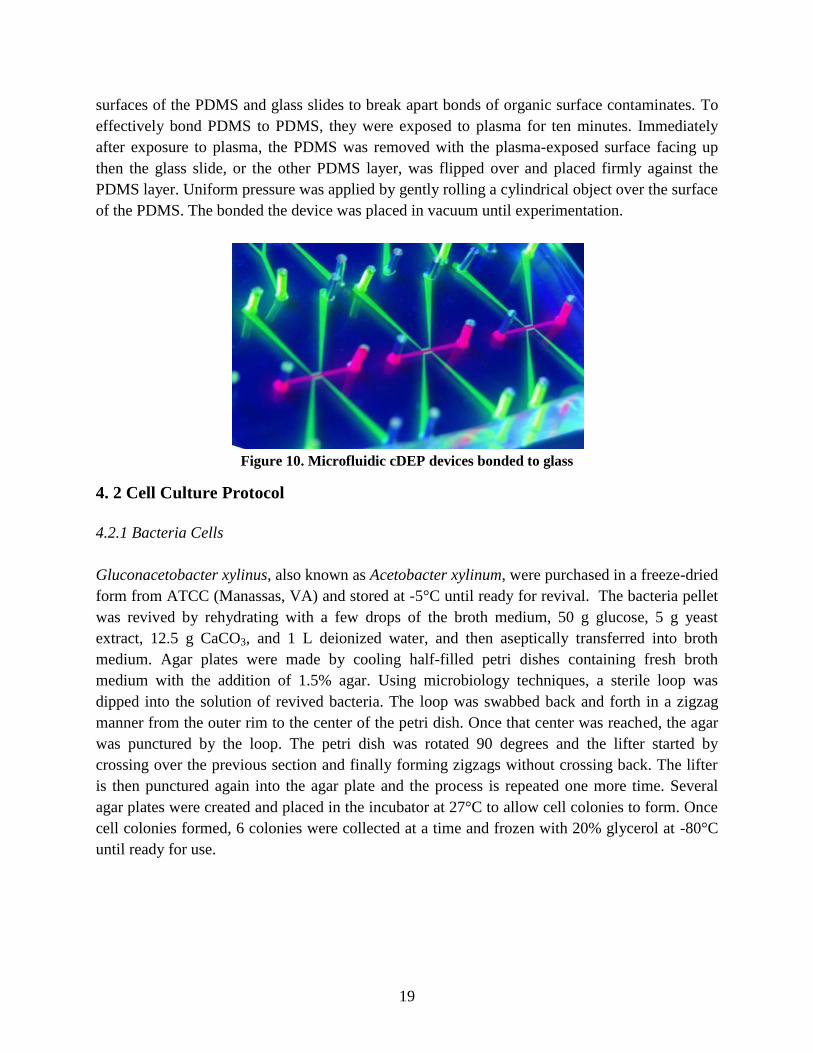
Figure 10. Microfluidic cDEP devices bonded to glass ................................................................ 19
Figure 11. Agar plate with zigzag lines showing the method for colonizing bacteria .................. 20
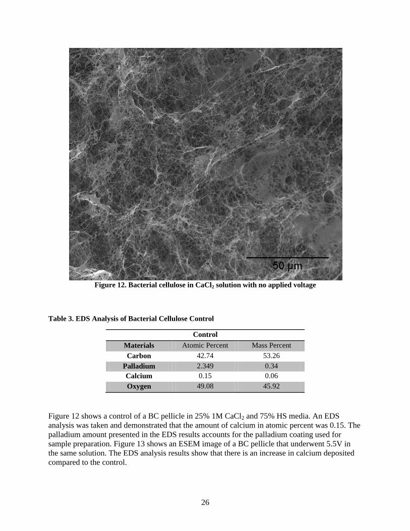
Figure 12. Bacterial cellulose in CaCl2 solution with no applied voltage .................................... 26
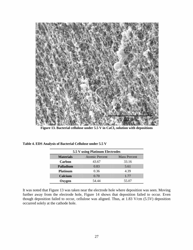
Figure 13. Bacterial cellulose under 5.5 V in CaCl2 solution with depositions ............................ 27
Figure 14. Bacterial cellulose image taken far from electrode hole showing alignment but no
deposition under the applied field ................................................................................................. 28
Figure 15. Bacterial cellulose pellicle showing the presence of calcium at one electrode hole ... 28
Figure 16. Schematic of meniscus pattern used in the experiments. Outer diameter is 46 mm with
a width of 10mm. Each channel was 50 microns wide and 50 microns deep............................... 29
Figure 17. Surface plot showing the electric field gradients to be highest towards the ends. The
plot was normalized using 1 Hz and 20 V. ................................................................................... 30
vi
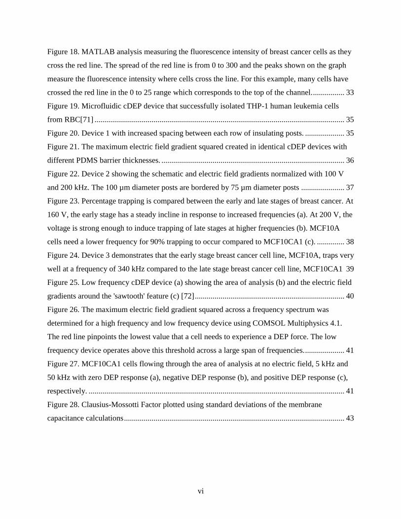
Figure 18. MATLAB analysis measuring the fluorescence intensity of breast cancer cells as they
cross the red line. The spread of the red line is from 0 to 300 and the peaks shown on the graph
measure the fluorescence intensity where cells cross the line. For this example, many cells have
crossed the red line in the 0 to 25 range which corresponds to the top of the channel. ................ 33
Figure 19. Microfluidic cDEP device that successfully isolated THP-1 human leukemia cells
from RBC[71] ............................................................................................................................... 35
Figure 20. Device 1 with increased spacing between each row of insulating posts. .................... 35
Figure 21. The maximum electric field gradient squared created in identical cDEP devices with
different PDMS barrier thicknesses. ............................................................................................. 36
Figure 22. Device 2 showing the schematic and electric field gradients normalized with 100 V
and 200 kHz. The 100 µm diameter posts are bordered by 75 µm diameter posts ...................... 37
Figure 23. Percentage trapping is compared between the early and late stages of breast cancer. At
160 V, the early stage has a steady incline in response to increased frequencies (a). At 200 V, the
voltage is strong enough to induce trapping of late stages at higher frequencies (b). MCF10A
cells need a lower frequency for 90% trapping to occur compared to MCF10CA1 (c). .............. 38
Figure 24. Device 3 demonstrates that the early stage breast cancer cell line, MCF10A, traps very
well at a frequency of 340 kHz compared to the late stage breast cancer cell line, MCF10CA1 39
Figure 25. Low frequency cDEP device (a) showing the area of analysis (b) and the electric field
gradients around the 'sawtooth' feature (c) [72] ............................................................................ 40
Figure 26. The maximum electric field gradient squared across a frequency spectrum was
determined for a high frequency and low frequency device using COMSOL Multiphysics 4.1.
The red line pinpoints the lowest value that a cell needs to experience a DEP force. The low
frequency device operates above this threshold across a large span of frequencies. .................... 41
Figure 27. MCF10CA1 cells flowing through the area of analysis at no electric field, 5 kHz and
50 kHz with zero DEP response (a), negative DEP response (b), and positive DEP response (c),
respectively. .................................................................................................................................. 41
Figure 28. Clausius-Mossotti Factor plotted using standard deviations of the membrane
capacitance calculations ................................................................................................................ 43

vii
List of Tables
Table 1. Components of the DEP Force: Units and Magnitudes .................................................. 14
Table 2. Electrical Properties Used for Numerical Modeling of Meniscus Design ...................... 24
Table 3. EDS Analysis of Bacterial Cellulose Control ................................................................. 26
Table 4. EDS Analysis of Bacterial Cellulose under 5.5 V .......................................................... 27
Table 5. Electrical Properties Used for Numerical Model of cDEP Devices [57] ....................... 34
Table 6. Measured Crossover Frequencies Normalized By Control and Conductivity of Buffer 42
Table 7. Calculated Membrane Capacitance of Breast Cancer Cells ........................................... 43

1
Chapter 1. Introduction
All particles will experience forces in response to applied electric fields as a consequence of their
intrinsic electrical properties [1]. This was first discovered by Reuss in 1809 when charged clay
particles suspended in a fluid migrated under an influence of an applied electric field which has
been known as electrophoresis [2]. Another facet of electrophoresis, simply by adding a non-
uniform electric field to a system, allowed uncharged particles to migrate in a fluid. The particle
response to this application of non-uniform fields was identified by Pohl and defined as
dielectrophoresis [3] and further presented in his 1978 book. Since then many applications have
used this electrokinetic technology, including industrial applications that deposit a patterned
coating of nanoparticles on a substrate using both DC and AC fields [4], environmental
applications that sort bacteria from water [5], and biomedical applications that aggregate cells for
co-culture systems [6].
This document describes two potential applications for using electrokinetics: tissue engineering
and cell separation of breast cancer cells. For tissue engineering, bacterial cellulose is explored
as a material for menisci purposes because of its hydroexpansive properties that resemble natural
menisci. The cellulose is produced by bacteria that secrete fibers as part of their metabolic
processes. Dielectrophoresis could be used as a method to control the motion of bacteria to create
a meniscus scaffold. Furthermore, a meniscus scaffold needs to be anchored into the
environment, and the addition of hydroxyapatite on the ends of the scaffold would promote
integration. Therefore, electrokinetics will be used to attempt deposition of calcium ions onto a
bacterial cellulose meniscus scaffold.
The second study for electrokinetics will be on understanding breast cancer cell response to
electric field gradients. The cell line progression model from the same parent cell, MCF10A, has
not been studied using electrokinetics and will provide insight on the capabilities for separating
breast cancer cells by stage. Previous work has proven to separate aggressive cells from early
and intermediate cells using dielectrophoresis [7]. However, the cell lines used were all from
different people. To study cancer detection techniques, it is ideal to use cells from the same
person. Therefore, the following work strives to separate stages of breast cancer cells by
designing and testing dielectrophoretic microdevices with different electric field gradients.

2
Chapter 2. Background & Significance
2.1 Directed Motion of Bacteria and Calcium Ions to Create a Meniscus
2.1.1 What is Bacterial Cellulose (BC)?
In the Philippines, a gel-like dessert exists, Nata de Coco, which is produced in coconut water
from bacteria cultures. The gel-like substance is referred to as bacterial cellulose and can be
generated by the species Acetobacter xylinum. The production of cellulose begins with the
movement of millions of bacteria cells in an acidic liquid at the air interface. The oxygen present
at the air-liquid interface allows for continuous cellulose production. Cellulose nanofibrils form
from cell metabolic secretions of glucose chains that entangle with other cellulose nanofibrils,
resulting in a complex network of fibers that forms a blanket of hydrophilic material [8, 9]. The
hydrophilic pellicle has been found to have great mechanical properties compared to other
polymers [10] and proven to be biocompatible [11]. BC can easily be molded into many shapes
if unagitated, therefore, has potential in medical applications including skin substitutes [12],
artificial blood vessels [13], bone[12, 14], and other tissue engineering projects. Some include
manipulating the bacterial cellulose porosity with wax particles to induce cell proliferation [15].
2.1.2 Alignment of Fibers Using Electric Fields
In the tissue engineering aspect, top-down fabrication of materials are limited on their feature
size and therefore clinical translations of the products are limited due to their inability to
reproduce on the nano or micro level. Complications with feature size arise when cells cannot
infiltrate scaffolds leading to cell proliferation failure. Bacterial cellulose is a potential
scaffolding material but is limited in its application due to their porous structure. The cellulose
naturally forms a tight, random network of fibers creating small pores that are not large enough
for cells to infiltrate. Furthermore, top-down fabrication techniques on bacterial cellulose such
as cutting it into a desired shape compromises the mechanical integrity. Therefore, any bottom-
up approach to fabricating larger pores and/or controlling fiber orientation would increase the
applications for bacterial cellulose in the medical field.

3
Figure 1. Bacterial cellulose (a) network of fibers viewed under SEM and (b) pellicle formed at
air/liquid interface
Sano et al. have been able to approach manufacturing issues by creating a bottom-up fabrication
method that controls the motion of the cellulose-producing bacteria. The Acetobacter xylinum are
one or two microns in size and therefore can feel the effects of electrokinetics [16]. Their size
assists with electrokinetics having a stronger effect than Brownian motion and negligible effects
from gravity [17]. Furthermore, since Acetobacter xylinum thrive in acidic solutions, their net
charge is negative [18]. The phenomena of electrophoresis, or motion of a charged particle
relative to a fluid under a uniform field, can play a dominant role having precise control over
bacteria cells and has been utilized to align bacterial cellulose fiber orientation. Using low DC
fields in the range of 0.25 V/cm to 1 V/cm, bacterial cells continued to secrete cellulose
nanofibrils and result in fiber alignment with their electrophoretic mobility estimated to be
4.68x10⁻⁹
m2Vs
-1. The ability to direct movement of bacteria potentially offers controlled fiber
alignment and pore size while maintaining mechanical integrity.
2.1.3 Deposition of Ions onto Bacterial Cellulose Fibers
The bacterial cellulose fiber network presents a good template to deposit or mineralize
nanoparticles for several biomedical applications. These include creating antimicrobial wound
dressings which are impregnated with silver nanoparticles [19] and bone regeneration by creating
a composite of cellulose and hydroxyapatite [12, 14]. Methods described for creating these
composites involve coating after the bacterial cellulose pellicle is formed using immersion
techniques. For bone mimics, the cellulose is first immersed in calcium solution then immersed
in a phosphorus solution to create a hydroxyapatite structure. Concerns arise when the porosity
of the cellulose limits the infiltration of the fluid into the pellicle resulting in solely surface
deposition.
Previous experiments in the Bioelectromechanical systems laboratory has shown to simplify
deposition processes. Using similar experimental protocols for aligning fibers, the deposition of
materials onto cellulose fibers using applied DC fields was also discovered. Altering electrode
materials and media constituents allowed deposition of free ions on to the cellulose fibers [20].
Deposition on individual cellulose fibers was seen using FESEM analysis and EDS verified
deposition of the following electrode materials: copper, graphite, aluminum, and platinum.

4
Phosphorus, a component not needed in the liquid medium, was added to the system before the
application of an electric field and FESEM verified the deposition of phosphorus. The electric
fields used during these experiments ranged from 0.15 V/cm to 1 V/cm. With this technique, one
can grow a BC pellicle while depositing desired materials onto individual fibers, thereby,
simplifying the fabrication process.
Figure 2. Bacterial cellulose coated with copper [20]
2.1.4 Significance of Bacteria Studies
Applying an electric field to bacterial cellulose resulted in two discoveries: alignment of fibers
and the deposition of ions. Both of these discoveries direct the field to fabricate a meniscus
scaffold. Studies have shown that bacterial cellulose is comparable to the collagen fibrils of
menisci; however, at high compression strains the ordered and arranged structure of the collagen
fibrils clearly surpasses the unorganized network of cellulose fibers [21]. Using an electric field
on the bacterial cellulose may orientate the fibers in the directions desired to mimic the collagen
structure and mechanical properties. The meniscus has an ordered layer structure mainly
containing circumferential fibers with some integrated radial fibers as seen in Figure 3.
Figure 3. A meniscus made of circumferential fibers with radial fibers integrated within the
network

5
To secure the manufactured bacterial cellulose meniscus, it should attach to the intercondyloid
fossa which is located between the condyles of the tibia. Therefore, the meniscus should be
fabricated with hydroxyapatite at the horns to initiate osteogenesis on the tibia. Hydroxyapatite, a
natural mineral component of bone, is composed of calcium and phosphate and is formulated
Ca5(PO4)3(OH). In this work, electric field gradients will be used to optimize design
considerations that will simplify the fabrication process. Meanwhile, deposition of calcium ions
on cellulose fibers will be tested and optimized. The ideal solution would be to create a meniscus
scaffold in only a few steps by applying an electric field for both alignment of fibers and
deposition of calcium ions, which would be followed by a phosphorus bath to create the
hydroxyapatite structure.
2.2 Separation of Breast Cancer Cells for Personalized Medicine
The motivation to create a technology that can personalize medicine for breast cancer
management and treatment is preceded by the negative results of blindly recommended
therapies. Oftentimes, these blindly recommended therapies lead to the immune system
becoming more resistive to further alternative treatments that if used originally could have killed
the cancer and/or prevented reoccurrence. Furthermore, patients with the same diagnosis treated
with the same therapeutic course may result with varying responses. The differences in their
responses depend on unidentified biomarkers, tumor microenvironment, tumor stage, and other
unknown factors which make up a cancerous cell’s genetic fingerprint [22]. This genetic
fingerprint creates a hurdle for personalizing medicine.
Personalizing medicine to manage and treat cancer will be optimized from experimental
therapeutic treatments in vitro using cancer cells from the patient. Studies have shown that
cancer from a primary tumor sheds cells into the blood stream even at early stages [23, 24]. The
cells known as circulating tumor cells (CTCs) circulate in the blood stream and may either be
attacked and killed by the immune system or initiate a secondary tumor site to begin metastasis.
More studies have shown that there is a direct correlation to the density of CTCs in the
peripheral blood and the progression of cancer [24-26]. Thus, the level of CTCs in blood can be
used as a predictor for patient prognosis [27]. Detection techniques that focus on finding CTCs
using blood samples provides a minimally invasive method to constantly screen for
reoccurrences as well as test for early stages of cancer. The following sections will discuss
current methods and approaches for detecting CTCs in vitro.
2.2.1 Techniques for Detecting Circulating Tumor Cells
The main challenge for detecting circulating tumor cells (CTCs) is the extremely low
concentration in blood (WBC 5-10106 mL
-1, RBC 5-910
6 mL
-1, and platelets 2.5-410
6 mL
-1),
as well as the identification of whether they are tumor initiating cells or not [28]. Several
technologies have been implemented to target these challenges, including the state of the art
magnetic-activated cell sorting (MACS) [29] and fluorescence-activated cell sorting (FACS)
[30], which are high throughput screening methods that label target cells using antibody
conjugated magnetic beads or fluorphore conjugated antibodies. The most reliable method for
CTC detection in blood is the CellSearch System, an automated enrichment and
immunocytochemical detection system first approved for use on monitoring patients with

6
metastatic breast cancer. The system uses magnetic beads coated with an antibody that targets
the epithelial cell adhesion molecule (EpCAM). Targeting CTCs with antibodies and labels has
its disadvantages of compromising cell structure and function as well as having limited
sensitivity. Prior knowledge of biomarkers are needed to target cells and even with negative
labeling, where undesired cells are targeted for removal, the sample may result in low yield and
purity [31]. A recent study questioned the sensitivity of CellSearch because the normal genotype
of invasive cancer is typically negative for the EpCAM expression, therefore the system will
give false negatives [32-34].
A method for CTC detection that excludes labeling is magnetophoresis. Separations based on
magnetophoresis use intrinsic magnetic properties of cells. When magnetophoretic separators
are scaled down to the microscale, red blood cells and white blood cells are sorted from whole
blood [35] and breast cancer cells are sorted from red blood cells [36]. The size was scaled-down
because macro-scale separators generated low magnetic flux gradients on the biological cells.
Another label-less detection method includes hydrodynamic sorting which is based on inertial
microfluidics. Park et al used a multi-orifice structure to move a particle laterally through inertial
lift force and vorticity and based the lateral movement on particle size [37]. However, the multi-
orifice structure alone does not sufficiently separate CTCs. Hydrodynamic sorting uses cell size
to separate particles from one another, but oftentimes cells are heterogeneous in their size even
though they are of the same cell type [38]. Therefore, Moon et al combined it with
dielectrophoresis to purify the output [39].
2.2.2 Dielectrophoresis
Dielectrophoresis (DEP), the motion of a particle due to its polarization in the presence of a non-
uniform electric field, can be used to differentiate between cells based on their intrinsic
properties [3, 40]. A particle’s response to a dielectrophoretic force may either be positive or
negative depending on the permittivity of the cell compared to the suspending fluid. A non-
uniform electric field polarizes the cell and the response time depends on the cell’s complex
permittivity, which is frequency dependent. Therefore, at some frequencies the cell’s may
respond to an applied force negatively or positively, i.e. repelled or attracted. DEP uses a cell’s
positive or negative response to selectively trap, separate, and sort polymer microspheres,
bacteria, and several types of eukaryotic cells in microchip applications [41-44]. The
disadvantage of using microdevices with interdigitated electrodes was the susceptibility of
electrode delamination and fouling during experimentation. Also, the electrode array patterned
on the bottom of the channel results in a DEP force that is weaker towards the top of the channel
where cells may not feel the force [45]. Turning up the electric field may increase the DEP force
at the top of the channel, but may cause cell damage to those closer to the electrode. To reduce
the disadvantages of traditional DEP microdevices and maintain the selectivity, insulator-based
dielectrophoretic (iDEP) devices were invented by Cummings et al [46]. The iDEP devices
simplified the fabrication process of DEP microdevices because the interdigitated electrodes
were replaced by insulating geometries, i.e. posts. A DC or AC electric field is applied through
electrodes that straddle the insulating structure array, consequently, creating non-uniform electric
field gradients around the posts. iDEP proved to be a successful adaptation and a robust
microdevice. Modifying microchannel geometry enhanced the performance of iDEP
microdevices [47-50] and lead to single cell trapping of MCF7 breast cancer cells [51],

7
separation of live and dead HeLa cells [52], separation and concentration of two species of live
bacteria [5], and separation of polystyrene beads in a multipart microdevice [53]. The
disadvantages for iDEP devices are the relatively high current flow within the channel causing
joule heating [51] and contamination from electrode/sample contact. When using
dielectrophoresis for CTC detection and enrichment, it is ideal to limit contamination from
electrode contact.
2.2.3 Contactless Dielectrophoresis
A fairly new rendition of dielectrophoresis is contactless dielectrophoresis (cDEP). The
microdevice design eliminates sample/electrode contact and proves to be ideal for handling
CTCs or any other precious cells. The metal electrodes are replaced by fluid electrode channels
filled with phosphate buffer saline PBS that are separated from the main channel by a
polydimethylsiloxane (PDMS) barrier. The insulating barriers capacitively couple the fluid
electrodes to the sample channel creating frequency dependent electric field gradients that varies
in response to geometrical and material properties of the device [54]. cDEP has been used to mix
0.5 µm fluorescent beads [55] and, more relevantly, has been used to separate live from dead
THP-1 human leukemia cells [56]. The following sections describe two types of devices that
operate at different frequency ranges with the original cDEP device working in high frequency
ranges.
2.2.3a High Frequency
The first few cDEP microdevices presented a main sample channel with electrode side channels
positioned directly above and below the area of cell capture. Numerical studies were
experimentally validated when below 100 kHz, cells did not respond to the applied electric field
gradients [56]. Furthermore, Shafiee et al found that frequencies above 700 kHz incurred
leakages of the side channels to the main sample channels. The minimum electric field gradient
squared on a particle necessary to induce movement was found to be on the order of 1012 [57]
.
Increasing the frequency and voltages improved cell capture, but cell lysis occurred when the
voltage exceeded a threshold [56]. A more selective cDEP microdevice resembled traditional
iDEP devices where in the main sample channel was an array of insulating posts. The electrode
side channels were positioned 20 microns above and below the section of the main sample
channel containing the array. This particular device was used in multiple experiments, first, to
trap live human leukemia cells around insulating posts while dead cells flowed through [56] and,
second, for the separation of breast cancer cells by stage [7].
8
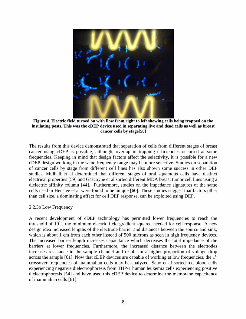
Figure 4. Electric field turned on with flow from right to left showing cells being trapped on the
insulating posts. This was the cDEP device used in separating live and dead cells as well as breast
cancer cells by stage[58]
The results from this device demonstrated that separation of cells from different stages of breast
cancer using cDEP is possible, although, overlap in trapping efficiencies occurred at some
frequencies. Keeping in mind that design factors affect the selectivity, it is possible for a new
cDEP design working in the same frequency range may be more selective. Studies on separation
of cancer cells by stage from different cell lines has also shown some success in other DEP
studies, Mulhall et al determined that different stages of oral squamous cells have distinct
electrical properties [59] and Gascoyne et al sorted different MDA breast tumor cell lines using a
dielectric affinity column [44]. Furthermore, studies on the impedance signatures of the same
cells used in Henslee et al were found to be unique [60]. These studies suggest that factors other
than cell size, a dominating effect for cell DEP response, can be exploited using DEP.
2.2.3b Low Frequency
A recent development of cDEP technology has permitted lower frequencies to reach the
threshold of 1012
, the minimum electric field gradient squared needed for cell response. A new
design idea increased lengths of the electrode barrier and distances between the source and sink,
which is about 1 cm from each other instead of 500 microns as seen in high frequency devices.
The increased barrier length increases capacitance which decreases the total impedance of the
barriers at lower frequencies. Furthermore, the increased distance between the electrodes
increases resistance in the sample channel and results in a higher proportion of voltage drop
across the sample [61]. Now that cDEP devices are capable of working at low frequencies, the 1st
crossover frequencies of mammalian cells may be analyzed. Sano et al sorted red blood cells
experiencing negative dielectrophoresis from THP-1 human leukemia cells experiencing positive
dielectrophoresis [54] and have used this cDEP device to determine the membrane capacitance
of mammalian cells [61].
9
2.2.4 Significance for Separating Stages of MCF10A cell line
The purpose of this research is to optimize cDEP microdevices to separate different stages of
breast cancer from the same parent cell line, MCF10A, so that they may be cultivated for
personalizing medicine purposes. Each stage of cancer will then be tested against different
therapeutic treatment options to determine the best one. It is possible that a mixture of different
therapies may be best to fight the cancer; therefore, separating them by stage is a foot forward
towards personalizing medicine. Previous work using high frequency cDEP studied the
separation efficiency for stages of breast cancer cells obtained from different people. The cDEP
device isolated aggressive MDA-MB-231 cells from intermediate and early stage cells, MCF7
and MCF10A, respectively [7]. The selectivity of the device can be improved by altering the
electric field gradients, but to mimic an ideal situation, the sample must come from the same
person. The progression of the MCF10A cell line continues with MCF10AT1 cells followed by
MCF10CA1 cells, which are early/intermediate and aggressive. Another cell line derived from
the MCF10AT1 line is the ductal carcinoma in situ (DCIS) cells which are intermediate cells.
The cell lines can be described more in detail from Miller et al and Santner et al [62, 63].

10
Chapter 3. Electrokinetic Theory
Electrokinetics is a family of effects that involves the motion of a liquid or particle within a
liquid in response to an external electric field. Most dielectric substances possess a surface
electric charge distribution that will attract ions of opposite sign (counter-ions) and repel ions of
like charge (co-ions) when brought into contact with an aqueous (polar) medium. This attractive
and repulsive process, when balanced by thermal diffusion, leads to the formation of the electric
double layer (EDL). The EDL is composed of two layers of ions. The first layer is known as the
Stern layer and consists of bound surface charge. The second layer consists of unbound charge,
formed by a balance between Coulombic attraction and diffusion, and is known as the diffuse
layer. The EDL forms the basis for which electrokinetic phenomena occur. If an electric field, for
example, is applied tangentially along a charged surface, the field will exert a force on the charge
and produce particle or liquid motion in the form of electrophoresis or electroosmosis,
respectively. As such, the electrokinetic phenomena presented here depend on two factors:
charge and an external electric field. The discussion below highlights the basic theory of these
two phenomena.
3.1 Electrokinetics in a Uniform Electric Field
The application of a voltage difference across some distance in a liquid will generate an electric
field, E
(1)
where, , is the applied voltage. The response of a particle within the fluid is dependent on the
distribution of the electric field. For example, a uniform direct current (DC) electric field can
induce particle movement if the particle surface contains bound charge, but will induce no
movement of a neutral particle. An influence by a uniform electric field on particle movement is
called electrophoresis. The charged particle will move towards the electrode that is of opposite
sign of the surface charge due to the Coulombic force attraction. Thus, a positively charged
particle will navigate towards a negatively charged electrode. The force on the particle is directly
proportional to the net charge of the cell, q.
(2)
Under a uniform DC field, the net forces on a particle are dependent on the motions induced by
electrophoresis and electroosmosis. For a fluid in a DC field, the electric field interacts with free
charges in the EDL, which forces this charged region into motion to drive fluid flow. Figure 5
shows the velocity profile of electroosmotic flow compared to laminar flow. Electroosmotic flow
moves at the same rate along the width of the channel minimizing sample dispersion while
pressure-driven flow causes the liquid in the center of the channel to move faster. Under a
uniform AC field, however, no net fluid motion is observed as the net effect of fluid movement
over one field cycle is zero [18].

11
Figure 5. Electroosmotic flow is more uniform across the width of the channel while pressure
driven flow is parabolic
Using Hückel’s equation [64], the sum of the electrophoretic mobility and electroosmotic
mobility is used to determine the electrokinetic velocity, , of a spherical cell, where
electrophoresis and electroosmosis are the only effects due to the applied electric field.
(3)
(4)
The electroosmotic mobility of a fluid under a uniform field may be calculated using
(5)
Where is the electrostatic potential between the ions in the EDL, is the viscosity of the fluid,
and is the permittivity of the fluid [64].
3.2 Electrokinetics in a Non-uniform Electric Field
Depending on the electric field distribution, more complex electrokinetic phenomena can occur.
One such type is known as dielectrophoresis (DEP). Unlike electrophoresis, DEP uses non-
uniform electric fields to induce particle motion. The key difference between DEP and
electrophoresis is that while electrophoresis relies on bound surface charge to produce a net body
force, the surface charge used to create DEP is induced by the electric field. As such, DEP can be
used to drive movement of a neutral particle, whereas electrophoresis requires a charged particle.
Hence, to adequately describe DEP one must consider how a particle polarizes under the
influence of a electric field. The polarization of the particle is taken into account by calculating
the net dipole force on a particle.

12
Figure 6. The net force on a dipole (a) and a polarized particle (b)
The figure shows two opposing charges separated by a distance, d. The arrows projecting off the
charges represent the electric field at those charges. At a random spatial distance, r, is the
location of the negative charge, -q, and at r+d is the location of the positive charge, +q. The
following equation describes the net force on the dipole:
(6)
The electric field can be expanded about the position of r using the vector Taylor series
expansion:
(7)
(8)
Since d is much smaller, only the zero and first term of the expansion is considered and results in
the following equation:
(9)
where p is the dipole moment. Using Coulomb’s law and the two-point dipole, the electric
potential, , can be calculated with a dipole moment p in a dielectric medium of
permittivity [1, 65]:
(10)
Using this equation, the effective field-induced dipole moment of a particle, p, can be determined
by comparing the potential of a dipole with the potential of an induced particle which is

13
calculated using a spherical single-shelled particle model [66]. This comparison can be made
because the ion distribution for a single-shelled model under an electric field resembles that of a
dipole. Other models including a homogeneous spherical particle, ellipsoidal single-shelled
particle, and multi-shell particle have all been used to determine the induced dipole term of
biological particles [18, 65, 67].
Figure 7. Single shell model of a cell comprised of a cytoplasm core and membrane as an outer shell
with radii r1and r2
The single-shell model represents the cytoplasm core and the cell membrane of a mammalian
cell. Using this model, each layer of the cell is modeled as an individual electrical shell as seen in
Figure 7. The induced electrical potential, , of the cytoplasm, cell membrane, and suspending
medium is calculated by solving the Laplace equation using two sets of boundary conditions:
(11)
(12)
And
(13)
(14)
where the first set of conditions state that the potential is continuous across the interfaces and the
second set describes the total current at the interfaces [65]. Once the induced electrical potential
for a single shell particle is determined it can be compared to Equation (10) to determine the
induced dipole moment of the particle
(15)

14
where is the effective complex permittivity that captures the charging characteristics of both
interfaces. Taking into consideration exponential time dependence for the electric field, the
instantaneous applied field at time t and location r is given by
(16)
where and is the real part of the complex phasor . This
notation accounts for the magnitude and phase of the electric field that induces a dipole moment
as the field is moving sinusoidally in time. The net dielectrophoretic force on the dipole can now
be determined by combining Equations (9), (15), and (16) as well as taking the time-average [1]
(17)
Using the vector relation, , and
knowing the electric field does not rotate gives us
; therefore,
the dielectrophoretic equation becomes
(18)
The cell in a fluid will also experience a drag force:
(19)
where is the viscosity of the particle and is the velocity. For cell motion to occur, the
magnitude of the must be greater than .
Table 1. Components of the DEP Force: Units and Magnitudes
radius
SI Units
COMSOL Units
Magnitude
3.3 Clausius-Mossotti (CM) Factor
The CM factor is a key component in determining the dielectrophoretic force on a particle and is
defined by the single-shell model as follows
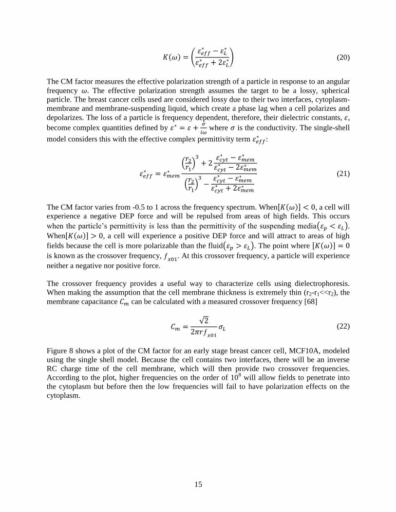
15
(20)
The CM factor measures the effective polarization strength of a particle in response to an angular
frequency The effective polarization strength assumes the target to be a lossy, spherical
particle. The breast cancer cells used are considered lossy due to their two interfaces, cytoplasm-
membrane and membrane-suspending liquid, which create a phase lag when a cell polarizes and
depolarizes. The loss of a particle is frequency dependent, therefore, their dielectric constants, ,
become complex quantities defined by
where is the conductivity. The single-shell
model considers this with the effective complex permittivity term :
(21)
The CM factor varies from -0.5 to 1 across the frequency spectrum. When , a cell will
experience a negative DEP force and will be repulsed from areas of high fields. This occurs
when the particle’s permittivity is less than the permittivity of the suspending media .
When , a cell will experience a positive DEP force and will attract to areas of high
fields because the cell is more polarizable than the fluid . The point where
is known as the crossover frequency,
. At this crossover frequency, a particle will experience
neither a negative nor positive force.
The crossover frequency provides a useful way to characterize cells using dielectrophoresis.
When making the assumption that the cell membrane thickness is extremely thin (r2-r1<<r2), the
membrane capacitance can be calculated with a measured crossover frequency [68]
(22)
Figure 8 shows a plot of the CM factor for an early stage breast cancer cell, MCF10A, modeled
using the single shell model. Because the cell contains two interfaces, there will be an inverse
RC charge time of the cell membrane, which will then provide two crossover frequencies.
According to the plot, higher frequencies on the order of 108 will allow fields to penetrate into
the cytoplasm but before then the low frequencies will fail to have polarization effects on the
cytoplasm.

16
Figure 8. The Clausius-Mossotti curve of an early stage breast cancer cell modeled using the single
shell model

17
Chapter 4. Methods and Materials
4. 1 Microdevice Fabrication
4.1.1 Polycarbonate Master Stamp Fabrication
Master stamps for cellulose fiber alignment were fabricated from polycarbonate boards that were
milled using a computer numerical controlling (CNC) machine. Fabrication was outsourced for
gratis by the mechanical engineering department at Virginia Tech. Rectangular channels were
milled into a variety of different lengths and widths, but similar depths.
Figure 9. Sample polycarbonate stamp to create channels
4.1.2 Silicon Wafer Master Stamp Fabrication
In the Micron cleanroom, a <100> grade silicon wafer (University Wafer, MA) was cleansed of
surface contaminates in BOE for 5 seconds then rinsed with deionized water and blown dry
using pressurized nitrogen. To prepare the surface for photoresist, hexamethyldisilizane (HDMS)
is used to promote adhesion and works best when HDMS is applied as a gas phase on a heated
substrate. Using a spinner, 5 drops of HDMS solution was spun on the wafer at 4000 rpm for 90
seconds then it was transferred to a hot plate set at 115°C for 90 seconds. The wafer was then
centered on the spinner again and a quarter-sized amount of AZ 9260 (AZ Electronics, NJ)
positive photoresist was poured onto the wafer and spun at 4000 rpm for 40 seconds. The wafer
was transferred to the hot plate to bake the photoresist at 115 °C for 30 seconds.
Upon curing of the photoresist, the MA-6 Mask Aligner (SUSS MicroTec, Germany) was used
to imprint the device design onto the photoresist covered wafer. The 2D device was designed
using AutoCAD Mechanical (AutoDesk, CA) and the high-quality photomask was printed by
CAD/Art Services, Inc. The photomask was printed with the emulsion side up; therefore,
features would be imprinted onto the device with the correct dimensions. The photomask is
taped onto a 4” x 4” glass substrate fitted for the mask aligner and placed in the aligner so that
the photomask comes in contact with the photoresist-covered wafer. The aligner was set to soft
contact at a distance of 40 µm with a UV exposure for 60 seconds. Following exposure to the

18
UV lamp, the silicon wafer was placed in a 2:1 AZ 400K (AZ Electronics) developer to water
solution for 30 seconds then rinsed with deionized water to remove the photoresist from the
microdevice features.
Once all the photoresist was removed from the features, the Deep Reactive Ion Etching (DRIE)
machine was used to etch the silicon wafer. The duration was calculated after measuring the rate
at which it etched between the time points of 3 minutes and 5 minutes using the Dektak (Bruker
AXS, WI). The Dektak measures the depth and is accurate for reading until a depth of 50 to 60
µm. Following DRIE etching, the wafer was placed in acetone for at least 5 minutes to remove
the remaining photoresist. Due to a scaffolding effect from the etch method, further processing of
the silicon wafer was needed to smooth the walls of the channels. Tetramethylammonium
hydroxide (TMAH), an anisotropic wet etchant of silicon, was heated to 70°C and used for the
removal of extra photoresist and the smoothing of the walls of the channels. The wafer was
placed in the heated TMAH for 5 minutes and then rinsed with deionized water followed by
pressurized nitrogen drying. A final coating on the silicon wafer was needed so that molds of
PDMS could be easily peeled off the silicon wafer. The coating used is PTFE, a fluoropolymer
with the chemical formula of C2F4. The DRIE applied the PTFE in gas form for 5 minutes.
4.1.3 Mold Formation of Devices
Molds of the devices were created using a SYLGARD 184 polydimethylsiloxane (PDMS) kit
from Dow Corning. A 10:1 ratio of the elastomeric base and hardener was measured out by
weight and mixed together by stirring vigorously. Depending on the size of the device, 25 grams
to 40 grams of polymer was used. The polymer was placed in vacuum for 30 minutes to remove
the bubbles formed from mixing. Meanwhile, the master stamp was wrapped in an aluminum foil
boat and placed on a hot plate at 115 °C. After 30 minutes in vacuum, the majority, if not all, of
the bubbles were removed, the polymer was slowly poured over the heated master stamp and left
to cure for about 15-20 minutes. After the polymer cured, it was removed from the heat source
and cooled for 5 minutes before peeling from the stamp. Holes for electrodes and for the inlets
and outlets were punctured in the PDMS using 1.5 mm punchers (Ted Pella, CA).
4.1.4 Bonding of PDMS Device to Glass Slide or PDMS
The PDMS mold was cleansed with a mixture of soap and water, deionized water, and ethanol
followed by pressurized air to dry off the PDMS. Further removal of any contamination was
accomplished using scotch tape. The same cleansing process was used for glass slides. A plasma
cleaner (Harrick Plasma, NY) was used to bond the PDMS to either glass or another PDMS
layer. The samples were placed surface-side up under vacuum for two minutes to create a low-
pressure gas chamber. After two minutes, the plasma was turned on for two minutes to ionize the
gas atoms using high frequencies, creating a magenta-colored glow, which in turn bombarded the
19
surfaces of the PDMS and glass slides to break apart bonds of organic surface contaminates. To
effectively bond PDMS to PDMS, they were exposed to plasma for ten minutes. Immediately
after exposure to plasma, the PDMS was removed with the plasma-exposed surface facing up
then the glass slide, or the other PDMS layer, was flipped over and placed firmly against the
PDMS layer. Uniform pressure was applied by gently rolling a cylindrical object over the surface
of the PDMS. The bonded the device was placed in vacuum until experimentation.
Figure 10. Microfluidic cDEP devices bonded to glass
4. 2 Cell Culture Protocol
4.2.1 Bacteria Cells
Gluconacetobacter xylinus, also known as Acetobacter xylinum, were purchased in a freeze-dried
form from ATCC (Manassas, VA) and stored at -5°C until ready for revival. The bacteria pellet
was revived by rehydrating with a few drops of the broth medium, 50 g glucose, 5 g yeast
extract, 12.5 g CaCO3, and 1 L deionized water, and then aseptically transferred into broth
medium. Agar plates were made by cooling half-filled petri dishes containing fresh broth
medium with the addition of 1.5% agar. Using microbiology techniques, a sterile loop was
dipped into the solution of revived bacteria. The loop was swabbed back and forth in a zigzag
manner from the outer rim to the center of the petri dish. Once that center was reached, the agar
was punctured by the loop. The petri dish was rotated 90 degrees and the lifter started by
crossing over the previous section and finally forming zigzags without crossing back. The lifter
is then punctured again into the agar plate and the process is repeated one more time. Several
agar plates were created and placed in the incubator at 27°C to allow cell colonies to form. Once
cell colonies formed, 6 colonies were collected at a time and frozen with 20% glycerol at -80°C
until ready for use.

20
Figure 11. Agar plate with zigzag lines showing the method for colonizing bacteria
To grow bacterial cellulose from the frozen state, a vial containing 6 colonies was retrieved from
the freezer and brought to room temperature. Once colonies were at room temperature, they were
transferred into a T-75 flask with 100 mL of media and placed in an incubator set at 27°C for
about 3 days until a cellulose pellicle formed at the air/liquid interface. If no apparent formation
of cellulose occurred then a new frozen vial was used and the process repeated. When a pellicle
formed at the liquid/air interface, the flask was shaken up to release bacteria cells from the
pellicle. Then 2 mL of media was removed and placed in a new container with 100 mL of fresh
media.
4.2.2 Bacteria Cell Media
The media used for all experiments was a modified Hestrin-Schramm medium. The constituents
of the media were a mix of the following in 1 liter of deionized water: 40 g fructose, 1 g
potassium phosphate (KH2PO4), 0.25 g magnesium sulfate heptahydrate (MgSO47H2O), 3.3 g
ammonium sulfate (NH4)2, 5 g yeast extract, 5 mL vitamin solution, 10 mL salt or trace metal
solution, and 20 mL corn steep liquor. The solution was sterile using filtration and the pH was
balanced to 5.5 with sodium hydroxide (NaOH).
4.2.3 Mammalian Cells
From a frozen state, a cell vial was removed from liquid nitrogen and sprayed with ethanol
followed by loosening the lid. The vial was immediately submerged (with the cap above
waterline) in a 37°C water bath until thawed (< 5 minutes). Under a cell hood, fresh 37°C media
was quickly introduced into the vial with a pipette and mixed in with the old media containing
DMSO. All contents of the vial were transferred into a 15 mL conical tube, which was then

21
topped with 10 mL of fresh media. The cells were centrifuged down at 120 rpm for 5 minutes
and old media was aspirated using a Pasteur pipette. Using a pipette, 5 mL of fresh warm media
was pipetted up and down to break up the cell clump that had formed while centrifuging and then
all of the media was transferred into a T-25 Flask for incubation at 37°C.
After cells adhered to the bottom of the flask, they were ready for passaging. Trypsin, PBS, and
media were placed in the 37°C water bath. After about 20 minutes, media was aspirated from
the cell flask by holding the flask upside down making sure the Pasteur pipette did not come in
contact with the adhered cells. The cells were washed with about 5-10 mL of PBS and then PBS
was aspirated. This process was repeated once more. Then 1-1.5 mL (for T-25 flask) or 3 mL
(for T-75 flask) of trypsin was added to the flask and placed in the incubator for 3-7 minutes, but
no more than 10 minutes. If some cells were still adhered to the bottom of the flask, then the
bottom or sides of the flask were lightly tapped until they become loose. About 5 mL of fresh
media (for T-25 flask) or 8 mL of fresh media (for T-75 flask) was added to neutralize the media
then transferred to a conical tube for centrifuging. The cells were spun down for 5 minutes and
mixture of media and trypsin was aspirated with a Pasteur pipette with care taken to not aspirate
the cell clump. Media was added to the clump of cells and pipetted up and down until the clump
was not apparent. A small amount from the inoculated media was taken and plated into a new T-
75 flask with 15mL of media (a T-25 flask will only have 5 mL of media). The amount taken
was dependent on current number of cells and how fast or slow the cells grew. The flask was
placed in the incubator until feeding, passaging, or experimentation.
Feeding occurred 2-3 days after the last passage or feeding time or whenever the media
drastically changed color. To feed the cells, media was heated up in the water bath and,
optionally, PBS was also heated. Once the fresh media was heated, the old media in the cell flask
was aspirated using the Pasteur pipette (making sure the cells were adhered to the bottom prior
to). If using the PBS, the cells were washed and then 15 mL of media was added.
For experiments, the cells were passaged as mentioned previously. However, after cells were re-
suspended in fresh media, one mL of inoculated media was removed and analyzed using the Vi-
Cell (Beckman Coulter, IN) to count the number of cells and average diameter. Once the cell
count was determined, some cells would be used to plate a new flask and the remaining cells
would be re-suspended in DEP buffer (8.5% sucrose wt/vol, 0.3% glucose wt/vol, 0.725%
DMEM/F12 wt/vol) [57] to create the appropriate concentration needed for the experiment.
Staining of cells was done either with Calcein AM or Calcein AM red/orange. About 4-6 µL of
stain was added into the conical tube with inoculated media and placed in a warm water bath for
10 minutes. The cells were spun down for 5 minutes and re-suspended in fresh DEP buffer. The
conductivity was measured using a SevenGo Pro conductivity meter (Mettler-Toledo,Inc., OH)
and if the conductivity was not near 100 µS/cm then they would be spun down for 5 minutes and
re-suspended until the desired conductivity was reached.

22
Note: Cells were not used for experiments after 10-15 passages. New cells were thawed and
cultured.
For freezing cells, it was best to use cells that have had only a low passage number. After
passaging, several cryovials were filled with 1 mL of the inoculated media (with no less than
1106 cells/mL) and then finally no more than 10% sterile DMSO was slowly added to each of
the cryovials. The DMSO helps prevent cell death. The cryovials were placed in a CoolCell®
(BIOCISION LLC, CA) then directly in a -80°C freezer to freeze at a rate of -1 degree per
minute.
4.2.4 Mammalian Cell Culture Media
The MCF10A and MCF10AT1 cells were cultured with 500 mL of DMEM/F12 (Invitrogen,
NY), 25 mL of horse serum (Invitrogen), 5 mL of penicillin/streptomycin (Invitrogen), 500 µL
of insulin (Sigma-Aldrich), 50 µL of cholera toxin(Sigma-Aldrich), 100 µL of epidermal growth
factor (Sigma-Aldrich) and 250 µL of hydrocortisone (Sigma-Aldrich). MCF10CA1 and DCIS
were cultured with DMEM/F12 and 5% horse serum. Additionally, 1% of syringe-filtered L-
glutamine (Invitrogen) was added every two weeks in each culture medium.
23
Chapter 5. Bacterial Cellulose Studies
5.1 Experimental Procedures
5.1.1 Applied DC fields for Controlling Deposition of Ions onto Cellulose Fibers
5.1.1a Device Setup for Deposition
Inoculated media was inserted into PDMS channels using 1000 µL pipette tips which were used
as reservoirs. Extra inoculated media was injected into each tip to equalize the flow in the
channel. The channels were 3 cm long and 0.5 cm wide. Platinum electrodes were placed in the
pipette tip reservoirs and connected to a DC power supply (Tenma Electronics, DE). The
experiments were left to run for 72 hours at several voltages: 3.5 V, 4 V, 5.5 V, 6 V, and 7 V.
5.1.1b Media Alterations for Ion Deposition
The culture media for the bacteria cells was altered using 25% 1M CaCl2 to 75% modified
Hestrin-Schramm (HS) Medium. For each experiment, 20 mL of the media mixture was
inoculated with 1 mL of bacteria.
5.1.1c Sample Preparation for ESEM
PDMS bonded to PDMS or glass was peeled apart to remove the pellicles formed during
experiments. The pellicles were placed in test tubes of deionized water, and then placed in the
sonicator for one hour at 60°C. Afterwards, the deionized water was removed and replaced with
fresh deionized water. The sample was then placed in liquid nitrogen and quickly removed and
placed in a freeze dryer (Labconco Corp., MO) for 48 hours. Once the samples were lyophilized,
they were cut and mounted onto an SEM specimen holder via copper tape. The samples were
sputter-coated with a mixture of platinum and palladium for 45 seconds to make the sample
conductive.
5.1.1d Alizarin Red Staining for Presence of Calcium
After the application of a DC field, samples that were not prepared for ESEM analysis were
submerged in deionized and shaken for 5 minutes in a conical tube. The deionized water was
replaced with fresh deionized water. Two drops of Alizarin Red Staining (Electron Microscopy
Sciences, PA), a tool to identify if calcium is present in a sample, was added to the submerged
pellicle for 10 minutes. The pellicle was then removed from the staining process and placed in
another conical tube with fresh deionized water and shaken for 5 minutes. Finally, the stained
pellicle was placed on a petri dish and analyzed. If the sample contained calcium, the areas
would turn a pinkish-red.

24
5.1.2 Applied AC Field Experiments to Create a Meniscus Scaffold
5.1.2a Preparation for Fluorescent Optical Microscopy
The devices used were PDMS molds bonded to glass with holes punctured on each end with 1.5
mm hole punchers (Ted Pella, Inc., CA). Bacteria cells were suspended in modified HS media
and stained using Baclight™ (Invitrogen, CA), so that they would be easily seen under the
fluorescent microscope. A pipette was used to inject inoculated media into the meniscus-shaped
mold until it was completely filled. Aluminum electrodes were placed directly into the punctured
holes and pressure flow was allowed to settle for several minutes before applying an AC electric
field.
5.1.2b Applied AC Fields on Fluorescent Bacteria
A function generator (GFG-3015, GW Instek, Taiwan) was used to apply an AC field to the
electrodes and was monitored using an oscilloscope (TDS-1002B, Tektronix, USA). Frequencies
used in these experiments were below 1 Hz and the magnitudes used were 10 V and below. An
inverted fluorescent microscope (Leica DMI 6000B, Leica Micros-systems, IL) equipped with a
camera (Leica DFC420, Leica Micro-systems, IL) was used to record video footage of bacteria
cell response to the applied AC fields.
5.1.2c Numerical Modeling of a 2D Meniscus under AC field
Using the AC/DC module in COMSOL Multiphysics 4.1., a geometry designed in AutoCAD
Mechanical was modeled to solve for the electric field distribution. This was accomplished by
solving for the potential distribution, , using the Laplace equation, The boundary
conditions used are prescribed uniform potentials at the inlet or outlet of the holes. The electrical
properties used are presented in Table 2.
Table 2. Electrical Properties Used for Numerical Modeling of Meniscus Design
Electrical Properties
of Materials
Electrical
Conductivity (S/m)
Relative Electrical
Permittivity
PDMS 0.831012
2.65
Water 5.510-6
80
5.2 Results and Discussion
The use of electrophoresis on Acetobacter xylinum cells is an innovative approach for
microweaving a potential tissue scaffold [16]. It is an alternative to top-down fabrication which
increases in cost when decreasing in feature size. Initial studies with electrophoresis allowed
potential for inexpensive bottom-up fabrication methods that would create feature sizes on the
nanoscale using the cellulose-producing bacteria. The following studies of controlling bacterial
cellulose with DC and AC fields lead to further understandings of cell and environment

25
response. The results presented here demonstrate the potential for creating a meniscus structure
using electric fields.
5.2.1 Deposition of Ions Using Applied DC Electric Fields.
The main goal for these experiments was to determine whether deposition of calcium could
occur simultaneously with fiber alignment to create a bottom-up approach for tissue engineering.
This would not only eliminate a step in the processing, but also improve the technique for
thoroughly depositing a material such as hydroxyapatite within the scaffold. As mentioned
previously in Chapter 2, current work to create a bacterial cellulose scaffold with hydroxyapatite
is limited to the cellulose surface.
The voltages applied during these experiments were to represent the electric fields within the
ranges given from a previous study [16]. However in these experiments, an electric field of 1.83
V/cm (5.5 V) provided the best results by producing cellulose for ESEM analysis. Voltages
above 5.5 V in the same chambers failed to produce a cellulose pellicle in the 6 attempts. A
higher electric field than 1.83 V/cm is a factor that may cause bacteria to stop producing
cellulose possibly because at these fields the velocity of the cell may be too high for secretion of
glucose chains [69] or other metabolic processes. At lower voltages the experiments failed to
show deposition.
26
Figure 12. Bacterial cellulose in CaCl2 solution with no applied voltage
Table 3. EDS Analysis of Bacterial Cellulose Control
Control
Materials Atomic Percent Mass Percent
Carbon 42.74 53.26
Palladium 2.349 0.34
Calcium 0.15 0.06
Oxygen 49.08 45.92
Figure 12 shows a control of a BC pellicle in 25% 1M CaCl2 and 75% HS media. An EDS
analysis was taken and demonstrated that the amount of calcium in atomic percent was 0.15. The
palladium amount presented in the EDS results accounts for the palladium coating used for
sample preparation. Figure 13 shows an ESEM image of a BC pellicle that underwent 5.5V in
the same solution. The EDS analysis results show that there is an increase in calcium deposited
compared to the control.
27
Figure 13. Bacterial cellulose under 5.5 V in CaCl2 solution with depositions
Table 4. EDS Analysis of Bacterial Cellulose under 5.5 V
5.5 V using Platinum Electrodes
Materials Atomic Percent Mass Percent
Carbon 43.67 33.16
Palladium 0.83 5.61
Platinum 0.36 4.39
Calcium 0.70 1.77
Oxygen 54.44 55.07
It was noted that Figure 13 was taken near the electrode hole where deposition was seen. Moving
further away from the electrode hole, Figure 14 shows that deposition failed to occur. Even
though deposition failed to occur, cellulose was aligned. Thus, at 1.83 V/cm (5.5V) deposition
occurred solely at the cathode hole.

28
Figure 14. Bacterial cellulose image taken far from electrode hole showing alignment but no
deposition under the applied field
Figure 15 further confirms these results when Alizarin red was used to detect calcium in the
pellicle with an applied field of 1.66 V/cm (5 V).
Figure 15. Bacterial cellulose pellicle showing the presence of calcium at one electrode hole

29
There was localized deposition seen on the BC pellicle. It is possible that once the cellulose was
growing and calcium ions in the local region of the cathode were deposited, the calcium ions in
other regions had difficulty migrating towards the cathode. Therefore, calcium was only
deposited locally instead of throughout the entire pellicle. If the experiment was set to run for
longer than 72 hours, then the amount deposited may have increased.
At lower electric fields, many of the experiments did not produce cellulose and when they did,
no deposition of calcium was seen. The experiments that failed to produce cellulose were a result
of the location: the fume hood. Since the experiments did not use much media, the exhaust of the
fume hood dried them up. With deposition failing to occur on the samples that did produce
cellulose, further studies were not completed at these electric fields.
Although the deposition was not seen to be uniform throughout the pellicle, deposition did occur
simultaneously with alignment of fibers. With that in mind, this technology has potential to be
used in creating a meniscus with aligned fibers and with hydroxyapatite ends to anchor in
position.
5.2.2 Bacteria Manipulation for Creating a Meniscus Using AC Fields
Since the bacterium, Acetobacter xylinum, creates a fiber network that is biocompatible, hydro-
expansive, and mechanically suitable, then the ideal tissue to mimic is the meniscus. Controlling
the orientation of the fiber network has potential with electric fields; however, the movement has
not been thoroughly studied using AC fields. The following study used a meniscus-shaped mold
to carry out experiments that would mimic future experiments. The design was used to guide the
bacteria in the circumferential direction that mimics the orientation of native menisci collagen
fibers. In this mold, channels were designed to be 50 microns wide and spaced apart by 150
microns of PDMS. The bacteria movement was monitored while adjusting frequencies and
voltage.
Figure 16. Schematic of meniscus pattern used in the experiments. Outer diameter is 46 mm with a
width of 10mm. Each channel was 50 microns wide and 50 microns deep

30
The results of the experiments proved that bacteria cells did respond to an AC field at low
frequencies such as 1 Hz. Higher frequencies were tested but no movement was observed. The
response of the bacteria at low frequencies showed that they moved backwards and forwards due
to electroosmotic flow. The movement did have a net motion, which is a result of a
dielectrophoretic force. It is safe to assume that the time-average velocity for the electroosmotic
flow is equal to zero.
A study on the electric field gradients created within the device was accomplished using
numerical modeling. The model uses a slightly different meniscus shape, but experimental
conditions were applied and the overall result is similar. Looking at the surface plot of the
electric field gradients, one can see that they are highest at the locations closest to the electrodes.
Also, the gradients are highest where the PDMS barriers end, which is in the shape of the upside
down ‘v’. The field minimum is presented in the center of the device. Therefore, bacteria cells on
the left side of the meniscus will have a net motion towards the left, whereas, the bacteria cells
on the right side will have a net motion to the right.
Figure 17. Surface plot showing the electric field gradients to be highest towards the ends. The plot
was normalized using 1 Hz and 20 V.
5.3 Future Work
As this was only a study on the response of bacteria cells to the fields, further work must be
completed to understand whether the mechanism of using these electric fields will be beneficial
in this field. First, the mechanism for depositing calcium ions needs to be studied further by
increasing deposition time from 48-72 hours to 7 days or more. From preliminary experiments, it
was noted that electrode material would degrade within several hours or days and therefore a
field would be terminated. Experiments on electrode coatings such as using Nafion could prevent
electrode ions from being removed and thus allow long term studies to occur. After deposition of
calcium ions, the cellulose will need to be immersed in a phosphate solution, such as simulated
body fluid [14], to initiate hydroxyapatite formation. Characterization will determine if the
hydroxyapatite formation embodies the bone structure and if it can promote osteogenesis.

31
Secondly, it was proven that bacteria cells respond to a DEP force under an AC electric field at
low frequencies. Since the experiments were observed under an optical microscope, cellulose
fibers were undetectable with the naked eye. Studies should be done over several days to see if
cellulose can grow under these conditions and whether fibers are growing within the center of
the meniscus. It may be possible that the DEP force will drive all the bacteria cells towards the
horns of the meniscus, which can create a dense network in that area compared to the center of
the meniscus. Altering the device geometry and electrode setup may solve the potential issue of
non-uniform density in the structure. However, device ideas that allow an open surface would be
ideal in creating the meniscus, since the cells need oxygen to produce the cellulose and the
cellulose needs to maintain its mechanical integrity. Even if the device contained a closed
surface, the geometry will only be replicable within the first few layers of the pellicle. Lastly,
mechanical testing on the bacterial cellulose will need to be performed to determine the effects
of electric fields on cellulose growth. The strength of aligned cellulose has not been tested
thoroughly enough to confirm any improvements to mechanical properties. Positive results of
this would be a major milestone in engineering meniscus scaffolds.

32
Chapter 6. Separation of Breast Cancer by Stage
6.1 Experimental Procedures
6.1.1 High Frequency Experimental Setup
Microdevices were placed in vacuum for 30 minutes prior to experimentation. Once the cells
were almost ready, the microdevice was removed from vacuum and prepped for experiments.
Pipette tips were placed in the inlets and outlets of the electrode side channels and phosphate
buffered saline (PBS) was injected into these side channels using a pipette. The microdevice was
viewed under the microscope to verify no leakage occurred. Thin-walled PTFE tubing (Cole-
Parmer Instrument Co., IL) was used and the ends were cut at an angle into one 3-inch piece and
one 6-inch piece. The 3-inch piece of tubing was inserted into the outlet of the device. Once the
cells were ready and suspended at a concentration of 106cells/mL, the 6-inch tubing was attached
to a 1 mL plastic syringe and used to draw up half a milliliter of cell suspension. The open end of
the tubing was inserted into the microdevice and the syringe was placed in a micro-syringe pump
(Harvard Apparatus, MA). The syringe pump applied flow rates as low as 0.02 mL/hr.
An AC electric field was created by a combination of waveform generation and amplification
equipment. The output signal of a function generator was amplified with a wideband power
amplifier (Amp-Line Corp., NY). The output voltage was enough to power a high-voltage
transformer (Amp-Line Corp.,NY) which was connected to the electrode side channels and an
oscilloscope to monitor the frequency and amplitude. Note: The transformer was placed on a
grounded surface and attached to devices using high-voltage wiring.
An inverted fluorescent microscope equipped with a camera was used to record 50 second videos
of the breast cancer cells flowing through the channel. The first two microdevices experimented
with were analyzed by quick observations. The final high frequency cDEP device was analyzed
using a MATLAB code. The code analyzed the intensity of the fluorescent cells flowing into the
device and out of the device. This measured the percent trapping of the cells.
6.1.2 Low Frequency Experimental Setup
The same process was used to prepare the microdevice for experimentation, but instead of one
outlet the microdevice contained two outlet channels. Each cell line was cultured in three
different flasks for each set of sample testing (n=3) to maintain viability throughout the
experiments. The concentration for each sample size was set around 3106 cells/mL and the
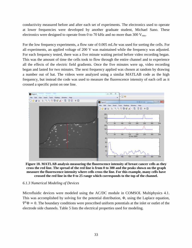
33
conductivity measured before and after each set of experiments. The electronics used to operate
at lower frequencies were developed by another graduate student, Michael Sano. These
electronics were designed to operate from 0 to 70 kHz and no more than 300 Vrms.
For the low frequency experiments, a flow rate of 0.005 mL/hr was used for sorting the cells. For
all experiments, an applied voltage of 200 V was maintained while the frequency was adjusted.
For each frequency tested, there was a five minute waiting period before video recording began.
This was the amount of time the cells took to flow through the entire channel and to experience
all the effects of the electric field gradients. Once the five minutes were up, video recording
began and lasted for two minutes. The next frequency applied was chosen at random by drawing
a number out of hat. The videos were analyzed using a similar MATLAB code as the high
frequency, but instead the code was used to measure the fluorescence intensity of each cell as it
crossed a specific point on one line.
Figure 18. MATLAB analysis measuring the fluorescence intensity of breast cancer cells as they
cross the red line. The spread of the red line is from 0 to 300 and the peaks shown on the graph
measure the fluorescence intensity where cells cross the line. For this example, many cells have
crossed the red line in the 0 to 25 range which corresponds to the top of the channel.
6.1.3 Numerical Modeling of Devices
Microfluidic devices were modeled using the AC/DC module in COMSOL Multiphysics 4.1.
This was accomplished by solving for the potential distribution, , using the Laplace equation,
. The boundary conditions were prescribed uniform potentials at the inlet or outlet of the
electrode side channels. Table 5 lists the electrical properties used for modeling.

34
Table 5. Electrical Properties Used for Numerical Model of cDEP Devices [57]
Electrical Properties
of Materials
Electrical
Conductivity (S/m)
Relative Electrical
Permittivity
DEP Buffer 0.01 80
PBS 1.4 80
PDMS 0.831012
2.65
6.2 Results and Discussion
Contactless dielectrophoretic devices were used for the following experiments to remove the
electrode/sample contact. Especially with handling breast cancer cells, the need to reduce
contamination is important when working with concentrations on the order of 10 circulating
tumor cells per mL of whole blood [70]. Any sort of contamination will affect culturing of these
cells. The following results walk through the design processes taken to change the selectivity of
the cDEP microdevices for breast cancer cells of different stage. It begins with alterations in the
high frequency devices, frequencies ranging from 100 kHz to 300 kHz, and ends with the newly
developed low frequency cDEP microdevice which can be used at frequencies of 70 kHz and
below.
6.2.1 High Frequency cDEP Experiments
There were three sets of devices that were used to study the breast cancer cell response to electric
field gradients. The designs were chosen to use the frequencies and voltages similar to previous
work [7]. In designing the models, the gradient of the electric field squared on the order of 1012
and above needed to be present to affect cells flowing through the channel. The first set of
experiments were initially conducted in a device used to successfully separate RBC and human
leukemia cells in the Bioelectromechanical systems laboratory at Virginia Tech [71].

35
Figure 19. Microfluidic cDEP device that successfully isolated THP-1 human leukemia cells from
RBC[71]
However, due to the inherited nature of breast cancer cells being a form of epithelial cells that
attach to surfaces and to each other easily, the cells fouled the device quickly. The fouling
disrupted fluid flow and the observed trapping of cells. To relieve clogging of the device, the
design was altered by increasing the space between each row of insulating posts.
Figure 20. Device 1 with increased spacing between each row of insulating posts.

36
For preliminary results of device 1, the early and early/intermediate cells, MCF10A and
MCF10AT1, were tested and values were recorded for onset and 90% of trapping under a flow
rate of 0.02 mL/hr. The onset of trapping was observed when cells began to show an obvious
attraction to the insulating posts by either slowing their velocity in the vicinity or by ‘sticking’
briefly to the post for a couple of seconds. The 90% trapping was observed when most of the
cells were attracted to the posts and formed pearl chains around them. Figure 19 shows the pearl
chain formation of THP-1 human leukemia cells around the insulating posts. The results showed
for both cell stages that the onset and 90% trapping were alike making the device not selective
enough. The frequencies and voltages recorded for the onset of the MCF10A cell was 320 kHz
and 95 V, while for the MCF10AT1 cells they were 320 kHz and 100 V. The frequency and
voltage noted for 90% trapping was exactly the same for both cell types. It is safe to state that
this device for breast cancer cells is not selective enough even though it may be for a mixture of
THP-1 cells and red blood cells. One of the main factors for selectiveness is the difference in cell
radius as pointed out in Equation 18 for dielectrophoretic force.
It was noted that the parameters used for these experiments were not exactly the same parameters
used in the work of Henslee et al with breast cancer cells [7]. It is possible that the barrier
thickness and depth has changed slightly due to processing. A quick study on the effect of barrier
thickness on the electric field gradient squared was modeled using COMSOL Multiphysics 4.1.
Figure 21 demonstrates the effect of a 10 micron barrier to a 20 micron barrier. The frequency
needed to reach the electric field gradient threshold decreases with decreasing barrier thickness,
so any slight differences in the thickness of the barrier may affect the frequency by 100 kHz or
more. Thus, it explains the differences in the frequencies used from previous work to current
work.
Figure 21. The maximum electric field gradient squared created in identical cDEP devices with
different PDMS barrier thicknesses.

37
A new device, device 2, was designed using two different insulating post sizes: 100 µm and 75
µm in diameter. The design was tested to determine whether the selectivity was an issue due to
clogging of the device around the corners of the electric field gradients. This design contains
large posts surrounded by small posts, which creates a higher gradient within the center of the
device. This would create a stronger force for attracting cells in the center of the device rather
than on the edges.
Figure 22. Device 2 showing the schematic and electric field gradients normalized with 100 V and
200 kHz. The 100 µm diameter posts are bordered by 75 µm diameter posts
The early/intermediate cell line and the aggressive cell line, MCF10AT1 and MCF10CA1, were
studied in this particular microdevice design. The fluid flow rate was set to 0.05 mL/hr. During
the experiments, the area of analysis was focused solely within the center of the device.
However, the response of the cells to this device did not change and the onset of trapping for
each cell line was exactly the same.
The final high frequency cDEP design, device 3, was designed with a smaller channel width. The
width of the sample channel and the number of post rows were reduced to improve fluid flow
and eliminate fouling. The early and late stage breast cancer cells, MCF10A and MCF10CA1,
were tested in the device at a flow rate of 0.02 mL/hr. The data was analyzed using a MATLAB
code described in the beginning of this chapter. Figure 23 shows at frequencies below 300 kHz,
MCF10A cells have an increasing % trapping trend at 160 V and 200 V. The aggressive cell line,

38
MCF10CA1, at 160 V seems to maintain a lower percent trapping range (10-30%) at higher
frequencies than the MCF10A cells. The percent trapping increases to 50-70% when increasing
voltage at those same frequencies. Overall at 160 V and 200 V, the MCF10A cells begin trapping
at much lower frequencies than the MCF10CA1 cells. Lastly, 90% of MCF10A cells can be
trapped at a lower frequency compared to MCF10CA1 cells.
Figure 23. Percentage trapping is compared between the early and late stages of breast cancer. At
160 V, the early stage has a steady incline in response to increased frequencies (a). At 200 V, the
voltage is strong enough to induce trapping of late stages at higher frequencies (b). MCF10A cells
need a lower frequency for 90% trapping to occur compared to MCF10CA1 (c).
Figure 24 demonstrates that at the same applied frequency and slightly different voltage, the
MCF10CA1 cells do not pearl chain as well as the MCF10A cell line. When pearl chaining
occurs, the dipole-dipole interaction between cells offers another binding force to a stationary
object like the interaction between the cell and insulating post caused by the electric field
gradients. The longer the chains, the more pronounced their interactions [1]. Therefore, fluid

39
flow cannot as easily break the interactions caused by the electric field gradients and carry the
cell passed this region. However, increasing the frequency or voltage for the MCF10CA1 cells
will eventually create the pearl chain effect. Thus, the cells inherently have different electrical
properties because for the same device it takes a different frequency and voltage to reach the
onset and 90% trapping efficiency or even to create the pearl chain effect.
Figure 24. Device 3 demonstrates that the early stage breast cancer cell line, MCF10A, traps very
well at a frequency of 340 kHz compared to the late stage breast cancer cell line, MCF10CA1
The issue continues to be selectivity of the device, and with higher frequencies this selectivity
seems limited if the particles have similar electrical properties. Using devices with frequencies
near the cell’s crossover frequency will help ascertain whether cDEP alone can be used for
separating out the different stages of breast cancer.
6.2.2 Low Frequency cDEP Experiments
A new cDEP device was recently designed to work at lower frequencies. The source electrodes
were positioned in the beginning of the device and spaced 1 cm away from the sink. The barriers
stretched alongside the main sample channel, located near the source electrodes, extend half a
centimeter long while the barriers near the sink electrodes stretch one and a half cm long. As
mentioned before in Chapter 2, the increased barrier length creates an increase in capacitance
which in turn decreases the total impedance of the barriers at low frequencies, thus, allowing this
device to operate at low frequencies. Figure 25a shows the electrodes, shaded in grey, are labeled
source and sink. The main sample channel does not necessarily have insulating posts to create
electric field gradients as was done for high frequency devices. Instead the microdevice contains
‘sawtooth’ structures that distort the electric field. Figure 25c shows the electric field gradients
with a maximum around these ‘sawtooth’ structures.

40
Figure 25. Low frequency cDEP device (a) showing the area of analysis (b) and the electric field
gradients around the 'sawtooth' feature (c) [72]
The device design altered the electric field gradients to increase at lower frequencies, especially
frequencies in which mammalian cells experience a crossover frequency, or a frequency in which
the cell response switches from positive DEP to negative DEP. Figure 26 compares the electric
field gradients for the low frequency device to a high frequency device. As mentioned before, the
electric field gradients must reach a minimum of 1012
for the cells to respond to the DEP force.
The graph proves that the low frequency cDEP device is capable of achieving this minimum
starting at frequencies of 3 Hz. In previous work, human leukemia cells, THP-1 cells, were
separated from red blood cells because the THP-1 cells experienced a positive DEP force
between 20 and 70 kHz [54]. The DEP force directed cells into streamlines closer to the maxima
of the electric field gradients and, therefore, caused them to flow across the top of the device. At
the same frequencies, the red blood cells experienced a negative DEP force and were repelled
from the maxima of the electric field gradients and therefore flowed towards the bottom of the
channel.

41
Figure 26. The maximum electric field gradient squared across a frequency spectrum was
determined for a high frequency and low frequency device using COMSOL Multiphysics 4.1. The
red line pinpoints the lowest value that a cell needs to experience a DEP force. The low frequency
device operates above this threshold across a large span of frequencies.
The breast cancer cells experienced similar behavior to the THP-1 cells. At low frequencies
including 5 kHz, all stages of breast cancer were repelled away from the ‘sawtooth’ structure.
Figure 27 demonstrates cell response under no electric field, 5 kHz, and 50 kHz.
Figure 27. MCF10CA1 cells flowing through the area of analysis at no electric field, 5 kHz and 50
kHz with zero DEP response (a), negative DEP response (b), and positive DEP response (c),
respectively.
Since the breast cancer cells were derived from the same cell line, MCF10A, it was expected that
their electrical properties were to be very similar. However, it was hypothesized that they could
be distinguishable at the first crossover frequency,
, using cDEP. At 30 kHz and above, all
cell lines were responding to some level of a positive DEP force by increasing cell-to-cell

42
interactions that became apparent with pearl chains forming as frequencies increased. The cell-
to-cell interactions can play a major role especially when determining the crossover frequency in
this device. At low flow rates and frequencies within the crossover range, the interactions may
attract more cells from one streamline into another, therefore, influencing where the cells cross
the line of analysis.
For these results two crossover frequencies were estimated using interpolation,
was
calculated based on the width of the channel and
was calculated based on the control
response. The cell’s response at the crossover frequency is neither negative nor positive, and the
observed response imitated the control. Each of these frequencies were then normalized to the
suspension conductivity which are comparable to results from Gascoyne et al where he
determined this ratio for several cell types including other breast cancer cell lines [44].
Table 6. Measured Crossover Frequencies Normalized By Control and Conductivity of Buffer
Stages of
Breast Cancer ƒx01
(Mhzm/S)
(Mhzm/S)
MCF10A 18.4 20.4 1.79 1.98
MCF10AT1 26.4 20.5 2.54 1.96
DCIS 21.4 21.8 1.99 2.03
MCF10CA1 18.84 13.75 1.75 1.28
For the early to intermediate stages, the estimated crossover frequencies were very similar. With
the added control measure, the crossover frequencies adjusted slightly almost to the point of
overlap. The control measured the movement of the cells when the electric field was turned off,
this was to determine whether fluctuations in fluid flow or cell concentration was skewing the
results. Therefore, these two crossover frequencies suggest that the measured values can vary
significantly with fluctuations in flow rate and cell concentration, limiting the selectivity. For
this specific device, separation cannot occur for the different stages of cancer. However, there is
potential for the MCF10CA1 cells to separate from the others since the crossover frequency is
much lower. This particular device was tested to separate the cells but small fluctuations had an
unfavorable effect, thereby, limiting its overall selectivity.
Using the results of the crossover frequency normalized by the control, the cell membrane
capacitance may be estimated for MCF10CA1 cells using Equation 22 and can be compared to
MCF10A estimated and reported membrane capacitance values.

43
Table 7. Calculated Membrane Capacitance of Breast Cancer Cells
(µS/cm) Radius (µm)
Membrane
Capacitance
(F/m2)
MCF10A [7] 12.54 100 9.25 0.0194
MCF10A 20.4 103 7.96 ±0.99 0.0143 ± 0.0036
MCF10AT1 20.5 104.5 6.81 ±0.90 0.0168 ± 0.0045
DCIS 21.8 107 7.79 ±0.62 0.0141 ± 0.0023
MCF10CA1 13.75 107 6.88 ±0.58 0.0255 ± 0.0042
The membrane capacitance was calculated using each cell’s radius with their standard
deviations. The CM factor is plotted with these standard deviations to determine if the membrane
of each cell plays a significant role in the electrical properties of the breast cancer cells. To plot
the single shell model of each cell, the cytoplasm conductivity was assumed to be 1 S/m and the
cytoplasm permittivity was assumed to be 50ε0. With these assumptions, the second crossover
frequency will not change and therefore is not shown.
Figure 28. Clausius-Mossotti Factor plotted using standard deviations of the membrane
capacitance calculations
According to the figure, the membrane capacitance for MCF10A, MCF10AT1, and DCIS is not
significant. With such a large variation in cell size, the first crossover frequency is not suitable
for separating these stages of breast cancer cells, especially within this current cDEP device. The

44
1st crossover frequencies are the same between early to intermediate stages of breast cancer,
suggesting that the membrane electrical properties are not significantly different enough to
produce a difference in DEP mobility and to drive effective separation. However, the potential to
separate MCF10CA1 cells from early and intermediate stages at these low frequencies remains
possible.
6.3 Future Work
Although the devices presented fell short of isolating different stages of breast cancer, the limits
have not been reached. Future preliminary studies should be done on these four different breast
cancer stages to determine their electric properties prior to moving on with testing the selectivity
of a device. The cells properties can be determined using electrorotation spectroscopy and
electroporation treatments which can measure, through direct analysis of the cell, the membrane
capacitance and conductance, as well as the polarization charging time.
Knowing at the first crossover frequency that the selectivity of these breast cancer cells is
unattainable using current cDEP designs only motivates for progress to be made studying either
the second crossover frequency or material aspects of the microfluidic device itself. According to
several authors, the membrane capacitance, cell radius, and media conductivity generally affect
the first crossover frequency, but the conductivity of a cell’s cytoplasm plays a role in the second
crossover frequency [38, 61]. Currently, experiments using cDEP at high frequencies in the
MHz range has not been studied, and perhaps for these breast cancer cells the cytoplasm
conductivities have more variation near the 2nd
crossover frequency.
Peering at the design aspect of the microdevice, the electric field gradients play a major role in
the selectivity of the cells. The devices used for ‘high frequency’ experiments were limited in
that range because of the material properties of PDMS. If another material with a higher
dielectric constant could be used to replace it, then the ‘high frequency’ devices may operate at
low frequencies especially near the crossover frequency. More experiments may also be
conducted with varying fluid conductivities and determining breast cancer cell stage response.
Another approach for using cDEP to separate breast cancer cells is to include a magnetic
component. Han et al previously explored magnetic fields to attract RBC to a center channel
while cancer cells were repelled to outer channels [36]. A preliminary experiment with cDEP
would be to incorporate a magnetic center channel filled with a solution of ferromagnetic
materials such as Fe, Ni, or Cobalt. Combining this with cDEP will help reduce the prep time
needed to remove white blood and cancer cells from blood.

45
Chapter 7. Conclusions
Electrokinetics has demonstrated its capability in two separate biomedical applications: tissue
engineering and cancer detection. The first application studied the effects of electric fields on
bacteria cells as well as calcium ions. In response to the electric field, calcium ions were able to
deposit simultaneously with cellulose growth. The benefit of using this technique is that
alignment of cellulose fibers can occur as nucleation sites for mineralization are forming.
Furthermore, there was localized deposition of ions at the electrode holes. The localization
allows for a meniscus design to form horns that will initiate osteogenesis to the tibia that will
anchor the structure. The other study in this application was determining the effects of an AC
field on bacteria cells. At low frequencies, bacteria were showing a response to electroosmosis
and DEP with a net motion caused by a DEP force created by the electric field gradients formed
from the meniscus design.
In the second application, dielectrophoresis in a contactless DEP device was studied as a method
for separating different stages of breast cancer all from the same person. Several geometries that
altered the electric field gradients were studied to determine their selectivity. With both ‘high’
and ‘low’ frequencies, the cells were incapable of being distinguished. The cell’s membrane
capacitance resulted in being very similar for each cell line and insignificant. Calculated
membrane capacitances overlapped simply by the variation of cell size within each cell line.
However, the most aggressive cell line showed potential for isolation from the other cells.
Therefore, the current cDEP devices were not selective enough to show this isolation. Future
work will be needed to study each cell’s cytoplasm response to electric fields, or in other words
studies at high frequencies that near each cell’s 2nd
crossover frequency.
46
References
[1] T. B. Jones, Electromechanics of Particles: Cambridge University Press, 1995.
[2] F. F. Ruess, Mem. Soc. Imperiale Naturalistes de Moscou, vol. 2, p. 327, 1809.
[3] H. A. Pohl, "The Motion and Precipitation of Suspensoids in Divergent Electric Fields,"
Journal of Applied Physics, vol. 22, pp. 869-871, 1951.
[4] S. Oh and O. Zhou, "Deposition Method for Nanostructure Materials," United States
Patent, 2008.
[5] B. H. Lapizco-Encinas, et al., "Insulator-based dielectrophoresis for the selective
concentration and separation of live bacteria in water," Electrophoresis, vol. 25, pp.
1695-1704, 2004.
[6] A. Sebastian, et al., "Tissue engineering with electric fields: Immobilization of
mammalian cells in multilayer aggregates using dielectrophoresis," Biotechnology and
Bioengineering, vol. 98, pp. 694-700, 2007.
[7] E. A. Henslee, et al., "Selective concentration of human cancer cells using contactless
dielectrophoresis," ELECTROPHORESIS, vol. 32, pp. 2523-9, Sep 2011.
[8] R. M. Brown, et al., "Experimental Induction of Altered Nonmicrofibrillar Cellulose,"
Science, vol. 218, pp. 1141-1142, 1982.
[9] S. Bielecki, et al., "Bacterial Cellulose," in Biopolymers Online, ed: Wiley-VCH Verlag
GmbH & Co. KGaA, 2005.
[10] S. Yamanaka, et al., "The structure and mechanical properties of sheets prepared from
bacterial cellulose," Journal of Materials Science, vol. 24, pp. 3141-3145, 1989.
[11] G. Helenius, et al., "In vivo biocompatibility of bacterial cellulose," Journal of
Biomedical Materials Research Part A, vol. 76A, pp. 431-438, 2006.
[12] S. A. Hutchens, et al., "Biomimetic synthesis of calcium-deficient hydroxyapatite in a
natural hydrogel," Biomaterials, vol. 27, pp. 4661-4670, Sep 2006.
[13] D. Klemm, et al., "Bacterial synthesized cellulose -- artificial blood vessels for
microsurgery," Progress in Polymer Science, vol. 26, pp. 1561-1603, 2001.
[14] K. A. Zimmermann, et al., "Biomimetic design of a bacterial cellulose/hydroxyapatite
nanocomposite for bone healing applications," Materials Science and Engineering: C,
vol. In Press, Corrected Proof.
[15] H. Bäckdahl, et al., "Engineering microporosity in bacterial cellulose scaffolds," Journal
of Tissue Engineering and Regenerative Medicine, vol. 2, pp. 320-330, 2008.
[16] M. B. Sano, et al., "Electromagnetically Controlled Biological Assembly of Aligned
Bacterial Cellulose Nanofibers," Annals of Biomedical Engineering, vol. 38, pp. 2475-
2484, Aug 2010.
[17] H. A. Pohl, Dielectrophoresis: The behavior of neutral matter in nonuniform electric
fields. Cambridge: Cambridge University Press, 1978.
[18] H. Morgan and N. G. Green, AC Electrokinetic: Colloids and Nanoparticles.
Hertfordshire: Research Studies Press LTD., 2003.
[19] T. Maneerung, et al., "Impregnation of silver nanoparticles into bacterial cellulose for
antimicrobial wound dressing," Carbohydrate Polymers, vol. 72, pp. 43-51, 2008.
[20] M. B. Sano, "Electromagnetic Control of Biological Assembly " Masters, Engineering
Science and Mechanics, Virginia Tech, Blacksburg, 2010.

47
[21] A. Bodin, et al., "Bacterial cellulose as a potential meniscus implant," Journal of Tissue
Engineering and Regenerative Medicine, vol. 1, pp. 406-408, 2007.
[22] E. A. Perez, "Breast Cancer Management: Opportunities and Barriers to an
Individualized Approach," The Oncologist, vol. 16, pp. 20-22, January 1, 2011 2011.
[23] T. Fehm, et al., "Cytogenetic Evidence That Circulating Epithelial Cells in Patients with
Carcinoma Are Malignant," Clinical Cancer Research, vol. 8, pp. 2073-2084, July 1,
2002 2002.
[24] E. Racila, et al., "Detection and characterization of carcinoma cells in the blood,"
Proceedings of the National Academy of Sciences, vol. 95, pp. 4589-4594, April 14, 1998
1998.
[25] W. J. Allard, et al., "Tumor Cells Circulate in the Peripheral Blood of All Major
Carcinomas but not in Healthy Subjects or Patients With Nonmalignant Diseases,"
Clinical Cancer Research, vol. 10, pp. 6897-6904, October 15, 2004 2004.
[26] J. G. Moreno, et al., "Changes in circulating carcinoma cells in patients with metastatic
prostate cancer correlate with disease status," Urology, vol. 58, pp. 386-392, 2001.
[27] M. Cristofanilli, et al., "Circulating Tumor Cells, Disease Progression, and Survival in
Metastatic Breast Cancer," New England Journal of Medicine, vol. 351, pp. 781-791,
2004.
[28] H. Lin, et al., "Disseminated and circulating tumor cells: Role in effective cancer
management," Critical Reviews in Oncology/Hematology, vol. 77, pp. 1-11, 2011.
[29] S. Miltenyi, et al., "High gradient magnetic cell separation with MACS," Cytometry, vol.
11, pp. 231-238, 1990.
[30] W. A. Bonner, et al., "Fluorescence Activated Cell Sorting," Review of Scientific
Instruments, vol. 43, pp. 404-409, 1972.
[31] A. Kumar, "Methods in cell separation for biomedical application: cryogels as a new
tool," Biomedical materials (Bristol), vol. 3, p. 034008, 2008.
[32] J. S. Ross and E. A. Slodkowska, "Circulating and Disseminated Tumor Cells in the
Management of Breast Cancer," American Journal of Clinical Pathology, vol. 132, pp.
237-245, August 1, 2009 2009.
[33] G. Deng, et al., "Enrichment with anti-cytokeratin alone or combined with anti-EpCAM
antibodies significantly increases the sensitivity for circulating tumor cell detection in
metastatic breast cancer patients," Breast Cancer Research, vol. 10, p. R69, 2008.
[34] A. M. Sieuwerts, et al., "Anti-Epithelial Cell Adhesion Molecule Antibodies and the
Detection of Circulating Normal-Like Breast Tumor Cells," Journal of the National
Cancer Institute, vol. 101, pp. 61-66, January 7, 2009 2009.
[35] K.-H. Han and A. B. Frazier, "Paramagnetic capture mode magnetophoretic
microseparator for high efficiency blood cell separations," Lab on a Chip, vol. 6, pp. 265-
273, 2006.
[36] K.-H. Han, et al., "Microsystems for isolation and electrophysiological analysis of breast
cancer cells from blood," Biosensors and Bioelectronics, vol. 21, pp. 1907-1914, 2006.
[37] J.-S. Park, et al., "Continuous focusing of microparticles using inertial lift force and
vorticity via multi-orifice microfluidic channels," Lab on a Chip, vol. 9, pp. 939-948,
2009.
[38] P. R. C. Gascoyne, et al., "Isolation of rare cells from cell mixtures by dielectrophoresis,"
ELECTROPHORESIS, vol. 30, pp. 1388-1398, 2009.
48
[39] H.-S. Moon, et al., "Continuous separation of breast cancer cells from blood samples
using multi-orifice flow fractionation (MOFF) and dielectrophoresis (DEP)," Lab on a
Chip, vol. 11, pp. 1118-1125, 2011.
[40] H. A. Pohl, "Some Effects of Nonuniform Fields on Dielectrics," Journal of Applied
Physics, vol. 29, pp. 1182-1188, 1958.
[41] N. G. Green, "Numerical determination of the effective moments of non-spherical
particles," Journal of physics. D, Applied physics, vol. 40, pp. 78-85, 2007.
[42] I. F. Cheng, "An integrated dielectrophoretic chip for continuous bioparticle filtering,
focusing, sorting, trapping, and detecting," Biomicrofluidics, vol. 1, p. 021503, 2007.
[43] R. S. Kuczenski, "Dielectrophoretic microfluidic device for the continuous sorting of
Escherichia coli from blood cells," Biomicrofluidics, vol. 5, p. 032005, 2011.
[44] P. R. C. Gascoyne, et al., "Dielectrophoretic separation of cancer cells from blood," IEEE
Transactions on Industry Applications, vol. 33, pp. 670-678, 1997.
[45] M. P. Hughes, "Strategies for dielectrophoretic separation in laboratory-on-a-chip
systems," Electrophoresis, vol. 23, pp. 2569-2582, 2002.
[46] E. B. Cummings and A. K. Singh, "Dielectrophoretic systems without embedded
electrodes," United States Patent, 2004.
[47] J.-S. Kwon, et al., "Improvement of microchannel geometry subject to electrokinesis and
dielectrophoresis using numerical simulations," Microfluidics and Nanofluidics, vol. 5,
pp. 23-31, 2008.
[48] J. McGraw Gregory, et al., "A Comparison of Insulator-Based Dielectrophoretic Devices
for the Monitoring and Separation of Waterborne Pathogens as a Function of
Microfabrication Technique," in Antiterrorism and Homeland Defense. vol. 980, ed:
American Chemical Society, 2007, pp. 133-157.
[49] J. Martínez-López, et al., "Characterization of electrokinetic mobility of microparticles in
order to improve dielectrophoretic concentration," Analytical and Bioanalytical
Chemistry, vol. 394, pp. 293-302, 2009.
[50] E. B. Cummings and A. K. Singh, "Dielectrophoresis in Microchips Containing Arrays of
Insulating Posts: Theoretical and Experimental Results," Analytical Chemistry, vol. 75,
pp. 4724-4731, 2003/09/01 2003.
[51] S. Bhattacharya, et al., "Insulator-based dielectrophoretic single particle and single
cancer cell trapping," ELECTROPHORESIS, vol. 32, pp. 2550-2558, 2011.
[52] C.-P. Jen and T.-W. Chen, "Selective trapping of live and dead mammalian cells using
insulator-based dielectrophoresis within open-top microstructures," Biomedical
Microdevices, vol. 11, pp. 597-607, 2009.
[53] R. C. Gallo-Villanueva, et al., "Separation of mixtures of particles in a multipart
microdevice employing insulator-based dielectrophoresis," ELECTROPHORESIS, vol.
32, pp. 2456-2465, 2011.
[54] M. B. Sano, et al., "Modeling and development of a low frequency contactless
dielectrophoresis (cDEP) platform to sort cancer cells from dilute whole blood samples,"
Biosensors and Bioelectronics, vol. 30, pp. 13-20, 2011.
[55] A. Salmanzadeh, et al., "Microfluidic mixing using contactless dielectrophoresis,"
ELECTROPHORESIS, vol. 32, pp. 2569-2578, 2011.
[56] H. Shafiee, et al., "Selective isolation of live/dead cells using contactless
dielectrophoresis (cDEP)," Lab on a Chip, vol. 10, pp. 438-445, 2010.

49
[57] H. Shafiee, et al., "Contactless dielectrophoresis: a new technique for cell manipulation,"
Biomedical Microdevices, vol. 11, pp. 997-1006, Tuesday, May 05, 2009 2009.
[58] H. Shafiee, "Marker-Free Isolation and Enrichment of Rare Cell types Including Tumor
Initiating Cells Through Contactless Dielectrophoresis," Doctor of Philosophy,
Engineering Science and Mechanics, Virginia Tech, Blacksburg, 2010.
[59] H. Mulhall, et al., "Cancer, pre-cancer and normal oral cells distinguished by
dielectrophoresis," Analytical and Bioanalytical Chemistry, vol. 401, pp. 2455-2463,
2011.
[60] A. Han, et al., "Quantification of the Heterogeneity in Breast Cancer Cell Lines Using
Whole-Cell Impedance Spectroscopy," Clinical Cancer Research, vol. 13, pp. 139-143,
January 1, 2007 2007.
[61] M. B. Sano, et al., "Contactless dielectrophoretic spectroscopy: Examination of the
dielectric properties of cells found in blood," ELECTROPHORESIS, vol. 32, pp. 3164-71,
2011.
[62] F. R. Miller, et al., "MCF10DCIS.com Xenograft Model of Human Comedo Ductal
Carcinoma In Situ," Journal of the National Cancer Institute, vol. 92, pp. 1185a-1186,
July 19, 2000 2000.
[63] S. J. Santner, et al., "Malignant MCF10CA1 Cell Lines Derived from Premalignant
Human Breast Epithelial MCF10AT Cells," Breast Cancer Research and Treatment, vol.
65, pp. 101-110, 2001.
[64] V. Tandon, et al., "Zeta potential and electroosmotic mobility in microfluidic devices
fabricated from hydrophobic polymers: 1. The origins of charge," ELECTROPHORESIS,
vol. 29, pp. 1092-1101, 2008.
[65] Z. R. Gagnon, "Cellular dielectrophoresis: applications to the characterization,
manipulation, separation and patterning of cells," ELECTROPHORESIS, vol. 32, pp.
2466-87, Sep 2011.
[66] K. V. Kaler and T. B. Jones, "Dielectrophoretic spectra of single cells determined by
feedback-controlled levitation," Biophys J, vol. 57, pp. 173-82, Feb 1990.
[67] A. Irimajiri, et al., "A dielectric theory of “multi-stratified shell” model with its
application to a lymphoma cell," Journal of Theoretical Biology, vol. 78, pp. 251-269,
1979.
[68] R. Pethig, "Review Article-Dielectrophoresis: Status of the theory, technology, and
applications," Biomicrofluidics, vol. 4, Jun 2010.
[69] M. R. Gretz, et al., "Cellulose biogenesis in bacteria and higher plants is disrupted by
magnetic fields," Naturwissenschaften, vol. 76, pp. 380-3, Aug 1989.
[70] S. Nagrath, et al., "Isolation of rare circulating tumour cells in cancer patients by
microchip technology," Nature, vol. 450, pp. 1235-1239, 2007.
[71] H. Shafiee, "Isolation and Enrichment of Human Leukemia Cancer Cells from Blood
Cells," Virginia Polytechnic Institute & State University, Blacksburg, 2011.
[72] M. B. Sano, "Theoretical Considerations of Biological Systems in the Presence of High
Frequency Electric Fields: Microfluidic and Tissue Level Implications," Ph.D. Candidate,
School of Biomedical Engineering and Sciences, Virginia Tech, Blacksburg, 2011.

50
Appendix A: MATLAB Code to Analyze Results from High Frequency cDEP Experiments
function image_analysis(file_name, varargin) % this function analyzes cDEP devices to measure the number of cells % entering and leaving a trapping region %there are two lines
clc %clear matlab command window (clean up)
% get input variables if any p = inputParser; p.addRequired('file_name'); p.addParamValue('entrance_x_offset', 0); p.addParamValue('entrance_y_offset', 0); p.addParamValue('exit_x_offset', 0); p.addParamValue('exit_y_offset', 0); p.addParamValue('entrance_scale', 1); p.addParamValue('exit_scale', 1); p.addParamValue('threshold', 95); p.addParamValue('line_length',440); p.addParamValue('video_length', 53); p.addParamValue('start_analysis', 10); p.addParamValue('end_analysis', 40); p.addParamValue('dir', 'G:\cDEP Experiments Breast Cancer\06-13-11\') p.parse(file_name, varargin{:}); p.Results;
%simplify variable names entrance_x_offset = p.Results.entrance_x_offset entrance_y_offset = p.Results.entrance_y_offset exit_x_offset = p.Results.exit_x_offset ; exit_y_offset = p.Results.exit_y_offset ; entrance_scale = p.Results.entrance_scale; exit_scale = p.Results.exit_scale; cell_threshold = p.Results.threshold; line_length = p.Results.line_length; video_length = p.Results.video_length; start_analysis = p.Results.start_analysis; end_analysis = p.Results.end_analysis; file_name = p.Results.file_name; dir = p.Results.dir;
line_length
% Parameters
%cut line for cell evaluation x(1,:) = [25 + entrance_x_offset, 25 + entrance_x_offset];
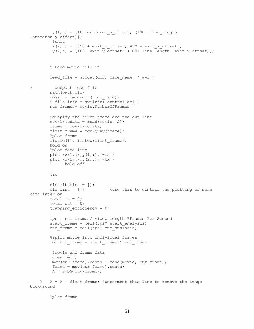
51
y(1,:) = [100+entrance_y_offset, (100+ line_length
+entrance_y_offset)]; %exit x(2,:) = [850 + exit_x_offset, 850 + exit_x_offset]; y(2,:) = [100+ exit_y_offset, (100+ line_length +exit_y_offset)];
% Read movie file in
read_file = strcat(dir, file_name, '.avi')
% addpath read_file path(path,dir) movie = mmreader(read_file); % file_info = aviinfo('control.avi') num_frames= movie.NumberOfFrames
%display the first frame and the cut line mov(1).cdata = read(movie, 2); frame = mov(1).cdata; first_frame = rgb2gray(frame); %plot frame figure(1), imshow(first_frame); hold on %plot data line plot (x(1,:),y(1,:),'-rx') plot (x(2,:),y(2,:),'-bx') % hold off
tic
distribution = []; old_dist = []; %use this to control the plotting of some
data later on total_in = 0; total_out = 0; trapping_efficiency = 0;
fps = num_frames/ video_length %Frames Per Second start_frame = ceil(fps* start_analysis) end_frame = ceil(fps* end_analysis)
%split movie into individual frames for cur_frame = start_frame:5:end_frame
%movie and frame data clear mov; mov(cur_frame).cdata = read(movie, cur_frame); frame = mov(cur_frame).cdata; A = rgb2gray(frame);
% A = A - first_frame; %uncomment this line to remove the image
background
%plot frame

52
if(mod(cur_frame, 2)==1) figure(3), imshow(A); hold on %plot data line plot (x(1,:),y(1,:),'-rx') plot (x(2,:),y(2,:),'-bx') hold off end
%% Analyze data here %original pixel data input_profile = improfile(A,x(1,:),y(1,:)); output_profile = improfile(A,x(2,:),y(2,:)); %plot pixel data figure(4) subplot(6,1,1),title(file_name),plot(input_profile, '-r') hold on, plot(output_profile, '-b'),plot([0
length(input_profile)], [cell_threshold cell_threshold]) hold off
%smoothed pixel data input = smooth(input_profile, 10); output = smooth(output_profile, 10);
%plot smothed pixel data subplot(6,1,2), if(mod(cur_frame, 2)==1) plot(input, '-r') hold on plot(output, '-b'), plot([0 length(output)], [cell_threshold
cell_threshold]), hold off ylim([0,cell_threshold]) end
%thresholded pixel data input_threshold = input>cell_threshold; output_threshold = output>cell_threshold;
%time analysis input_time(cur_frame) = sum(input_threshold); output_time(cur_frame) = sum(output_threshold);
%plot time analysis subplot(6,1,3) plot(input_time, '-r'); hold on plot(output_time, '-b') title(file_name); hold off
%trapping efficiency analysis total_in = total_in + sum(input_threshold)

53
total_out = total_out + sum(output_threshold) trapping_efficiency = ((total_in - total_out) / total_in) * 100;
subplot(6,1,5) bar([total_in, total_out]) set(gca,'XTickLabel',{'cells in', 'cells out'})
subplot(6,1,6) bar(trapping_efficiency) ylim([0,100]) set(gca,'XTickLabel',{'trapping efficiency'}) title(int2str(trapping_efficiency))
%input distribution if ~exist('input_distribution') input_distribution = zeros(size(input_threshold)); input_distribution = input_distribution + input_threshold; old_input_dist = input_distribution; else input_distribution = input_distribution + input_threshold; end
%output distribution if ~exist('output_distribution') output_distribution = zeros(size(output_threshold)); output_distribution = output_distribution + output_threshold; old_output_dist = output_distribution; else output_distribution = output_distribution + output_threshold; end
if ( isequal(input_distribution,old_input_dist) &&
isequal(output_distribution, old_output_dist)) %dont replot if distributions haven't changed
else %if distribution has changed, plot subplot(6,1,4)
plot(input_distribution, '-r'); hold on plot(output_distribution, '-b') title(file_name); hold off % pause(.1) end
old_input_dist = input_distribution; old_output_dist = output_distribution;
end hold off toc %

54
size(input_distribution) size(output_distribution) size(input_time) size(output_time) size(total_in) size(total_out) size(trapping_efficiency)
directory = 'output files/'; file = strcat(dir,directory,file_name, '.txt'); xLtitle = {'input_distribution ', 'output_distribution ', 'input_time
', 'output_time ', 'total_in ', 'total_out ', 'trapping_efficiency '} xLdata = padcat(input_distribution, output_distribution,
input_time', output_time', total_in', total_out', trapping_efficiency'); size(xLtitle) size(xLdata) % data = [xLtitle; xLdata] % xlswrite(file, xLtitle, 'Sheet1', 'A1'); save(file, 'xLdata', '-ascii') % file = strcat(dir, directory,file_name, '.mat'); save(file, 'input_distribution', 'output_distribution', 'input_time',
'output_time', 'total_in', 'total_out', 'trapping_efficiency', '-mat')
beep; pause(1);beep; end
function analyze_all % Calls the imagine_analysis function for each video clear all; close all; clc
image_analysis('340 160V - 1','line_length', 280,'entrance_y_offset',75,
'exit_x_offset',8,'exit_y_offset',80,'threshold', 70,'dir', 'G:\cDEP
Experiments Breast Cancer\06-13-11\')

55
Appendix B: MATLAB Code to Analyze Results from Low Frequency cDEP Experiments
function image_analysis(file_name, x_offset,y_offset, threshold)
% close all clc % clear all
cell_threshold = 80; switch nargin case 1 x_offset=0; y_offset=0;
case 2 y_offset=0;
case 4 cell_threshold = threshold end
% Parameters display_every = 100; %cut line for cell evaluation x2 = [450+x_offset,450+x_offset]; y2 = [155+y_offset, 460+y_offset];
% Read movie file in %dir = 'H:\cDEP Experiments Breast Cancer\08-11-11\'; % dir = 'G:\cDEP Experiments Breast Cancer\08-13-11\'; %dir = 'F:\cDEP Experiments Breast Cancer\08-15-11\'; dir = 'H:\cDEP Experiments Breast Cancer\08-16-11\';
read_file = strcat(dir, file_name, '.avi')
% addpath read_file path(path,dir) movie = mmreader(read_file); % file_info = aviinfo('control.avi') num_frames= movie.NumberOfFrames
frame = read(movie, 1); A = rgb2gray(frame); first_frame = A; % %plot frame figure(1), imshow(A); hold on

56
%plot data line plot (x2,y2,'-rx') % hold off
start_frame = 1; end_frame =num_frames; tic
distribution = []; old_dist = []; %use this to control the plotting of some
data later on
%split movie into individual frames for cur_frame = start_frame:10:end_frame-100
%movie and frame data % clear mov; % mov(cur_frame).cdata = read(movie, cur_frame); % frame = mov(cur_frame).cdata; frame = read(movie,cur_frame); A = rgb2gray(frame); % A = A - first_frame; %This removes the background % %plot frame if(mod(cur_frame, display_every)==1) figure(3), imshow(A);
hold on %plot data line plot (x2,y2,'-rx') hold off end
% xlabel(strcat(int2str(cur_frame), '/', int2str(end_frame)));
%% Analyze data here %original pixal data c = improfile(A,x2,y2);
%plot pixel data if(mod(cur_frame, display_every)==1) figure(4) subplot(4,1,1),title(file_name),plot(c) hold on, plot([0 length(c)], [cell_threshold cell_threshold]) hold off end
%smoothed pixel data output = smooth(c, 10);
%plot smoothed pixel data subplot(4,1,2), if(mod(cur_frame, display_every)==1) plot(output, '-r'), hold on

57
plot([0 length(output)], [cell_threshold cell_threshold]), hold
off end
%threshold pixel data threshold = output>cell_threshold;
if(size(distribution) == 0) distribution = zeros(size(threshold)); distribution = distribution + threshold; old_dist = distribution; else distribution = distribution + threshold; end
if (distribution == old_dist)
else subplot(2,1,2) plot(distribution, '-b'); title(file_name); hold off end old_dist = distribution; end hold off toc
directory = 'output files/'; file = strcat(dir,directory,file_name, '.txt'); save(file, 'distribution', '-ascii')
file = strcat(dir,directory,file_name, '.mat'); save(file, 'distribution', '-mat')
beep; pause(1);beep; end
function analyze_all %Calls the image_analysis function to analyze the each clear all; close all;
%% AT1 08-16-11 %image_analysis('10 kHz 200V AT1_3',-70,40,20) %image_analysis('20 kHz 200V AT1_3',-70,40,20) %image_analysis('20 kHz 200V AT1_3 short',-70,40,20) %image_analysis('30 kHz 200V AT1_3',-70,40,20) %image_analysis('40 kHz 200V AT1_3',-70,40,20) %image_analysis('50 kHz 200V AT1_3',-70,40,20) %image_analysis('60 kHz 200V AT1_3',-70,40,20) %image_analysis('70 kHz 200V AT1_3',-70,40,20) %image_analysis('Control AT1_3',-70,40,20)

58
Appendix C: MATLAB Code for Plotting the Clausius-Mossotti Curve
function model_used_for_AndreaThesis_plus_minus clc clear all close all w=2*pi*logspace(2,9,100); w2 = w.*w; rnorm= 9.25e-6; %radius of MCF10A from Henslee et al rn10Ap=7.96e-6; %radius of MCF10A found by Andrea rn10Am=7.96e-6; rn10A=7.96e-6; rAT1=6.81e-6; %radius of MCF10AT1 found by me(Andrea) rAT1p=6.81e-6; %radius of MCF10AT1 found by me(Andrea) rAT1m=6.81e-6; %radius of MCF10AT1 found by me(Andrea) rDCIS=7.79e-6; %radius of DCIS found by me(Andrea) rDCISp=7.79e-6; %radius of DCIS found by me(Andrea) rDCISm=7.79e-6; %radius of DCIS found by me(Andrea) rCA1=6.88e-6; %radius of MCF10CA1 found by me(Andrea) rCA1p=6.88e-6; %radius of MCF10CA1 found by me(Andrea) rCA1m=6.88e-6; %radius of MCF10CA1 found by me(Andrea)
conductivity = 0.01;% [S/m]
% Calculate C-M for each cell for i=1:length(conductivity) knorm(i,:) = norm(rnorm, w,conductivity(i)); kn10A(i,:) = n10A(rn10A, w,conductivity(i)); kn10Ap(i,:) = n10Ap(rn10Ap, w,conductivity(i)); kn10Am(i,:) = n10Am(rn10Am, w,conductivity(i)); kAT1(i,:) = AT1(rAT1, w,conductivity(i)); kAT1p(i,:) = AT1p(rAT1p, w,conductivity(i)); kAT1m(i,:) = AT1m(rAT1m, w,conductivity(i));
kDCIS(i,:) = DCIS(rDCIS, w,conductivity(i)); kDCISp(i,:) = DCISp(rDCISp, w,conductivity(i)); kDCISm(i,:) = DCISm(rDCISm, w,conductivity(i)); kCA1(i,:) = CA1(rCA1, w,conductivity(i)); kCA1p(i,:) = CA1p(rCA1p, w,conductivity(i)); kCA1m(i,:) = CA1m(rCA1m, w,conductivity(i)); end
% Plot the CM factor based on membrane capacitance std deviation pos and neg figure('name', 'CM of Breast Cancer Cells by Stage'); semilogx(w/(2*pi),knorm(1,:), 'k', w/(2*pi), kn10Ap(1,:), 'r',w/(2*pi),
kn10Am(1,:), 'r', w/(2*pi), kAT1p(1,:), 'b',w/(2*pi), kAT1m(1,:), 'b',
w/(2*pi), 0, 'k', w/(2*pi), kDCISp(1,:),'g',w/(2*pi),
kDCISm(1,:),'g',w/(2*pi), kCA1p(1,:),'c',w/(2*pi), kCA1m(1,:),'c')
xlabel('Frequency (Hz)') ylabel('Re[K(\omega)]')

59
hold off
end
function Knorm= norm(r, w, sig_media) %this function returns an array of values for the Clausius-Mossotti factor %for 10Aref Cells based on the conductivity of the media % r = cell radius % w = angular frequency % sig_media = conductivity of the media rnorm=9.25e-6; w=2*pi*logspace(2,9,100); w2 = w.*w; %radial frequency squared e0=8.85e-12; e1=80*e0; sig1=100e-4; %sigma of DEP buffer ~100uS/cm ec=50*e0; sigc=1; Cm = 0.0194; %value from Henslee et al tm=Cm*rnorm/sigc; tc=ec/sigc; t1=e1/sig1; tmstar=Cm*rnorm/sig1; j=sqrt(-1); t1tm=t1*tm; tctms=tc*tmstar; top=w2.*(t1tm-tctms)+j.*w.*(tmstar-t1-tm)-1; bottom=w2.*(2*t1tm+tctms)-j.*w.*(tmstar+2*t1+2*tm)-2; Knorm=(-1)*top./bottom; size(Knorm); end
function Kn10Ap =n10Ap(r,w,sig_media) %this function returns an array of values for the Clausius-Mossotti factor %for 10Ap std dev (positive)Cells based on the conductivity of the media w2 = w.*w; %radial frequency squared e0=8.85e-12; e1=80*e0; sig1=103e-4; %sigma of DEP buffer ~100uS/cm ec=50*e0; sigc=1; Cm = 0.01269; %value calculated tm=Cm*r/sigc; tc=ec/sigc; t1=e1/sig1; tmstar=Cm*r/sig1; j=sqrt(-1); t1tm=t1*tm; tctms=tc*tmstar; top=w2.*(t1tm-tctms)+j.*w.*(tmstar-t1-tm)-1; bottom=w2.*(2*t1tm+tctms)-j.*w.*(tmstar+2*t1+2*tm)-2; Kn10Ap=(-1)*top./bottom; size(Kn10Ap); end
function Kn10Am =n10Am(r,w,sig_media)

60
%this function returns an array of values for the Clausius-Mossotti factor %for 10Ap std dev (negative) Cells based on the conductivity of the media w2 = w.*w; %radial frequency squared e0=8.85e-12; e1=80*e0; sig1=103e-4; %sigma of DEP buffer ~100uS/cm ec=50*e0; sigc=1; Cm = 0.0163; %value calculated tm=Cm*r/sigc; tc=ec/sigc; t1=e1/sig1; tmstar=Cm*r/sig1; j=sqrt(-1); t1tm=t1*tm; tctms=tc*tmstar; top=w2.*(t1tm-tctms)+j.*w.*(tmstar-t1-tm)-1; bottom=w2.*(2*t1tm+tctms)-j.*w.*(tmstar+2*t1+2*tm)-2; Kn10Am=(-1)*top./bottom; size(Kn10Am); end
function KAT1p= AT1p(r, w, sig_media) %this function returns an array of values for the Clausius-Mossotti factor %for 10AT1 (pos std dev) cells based on the conductivity of the media w2 = w.*w; %radial frequency squared e0=8.85e-12; e1=80*e0; sig1=104.5e-4; %sigma of DEP buffer ~100uS/cm ec=50*e0; sigc=1; Cm = 0.01488; %value calculated tm=Cm*r/sigc; tc=ec/sigc; t1=e1/sig1; tmstar=Cm*r/sig1; j=sqrt(-1); t1tm=t1*tm; tctms=tc*tmstar; top=w2.*(t1tm-tctms)+j.*w.*(tmstar-t1-tm)-1; bottom=w2.*(2*t1tm+tctms)-j.*w.*(tmstar+2*t1+2*tm)-2; KAT1p=(-1)*top./bottom; size(KAT1p); end
function KAT1m= AT1m(r, w, sig_media) %this function returns an array of values for the Clausius-Mossotti factor %for 10AT1 (negative std dev) Cells based on the conductivity of the media w2 = w.*w; %radial frequency squared e0=8.85e-12; e1=80*e0; sig1=104.5e-4; %sigma of DEP buffer ~100uS/cm ec=50*e0; sigc=1; Cm = 0.01941; %value calculated

61
tm=Cm*r/sigc; tc=ec/sigc; t1=e1/sig1; tmstar=Cm*r/sig1; j=sqrt(-1); t1tm=t1*tm; tctms=tc*tmstar; top=w2.*(t1tm-tctms)+j.*w.*(tmstar-t1-tm)-1; bottom=w2.*(2*t1tm+tctms)-j.*w.*(tmstar+2*t1+2*tm)-2; KAT1m=(-1)*top./bottom; size(KAT1m); end
function KDCISp= DCISp(r, w, sig_media) %this function returns an array of values for the Clausius-Mossotti factor %for DCIS (positive std dev) cells based on the conductivity of the media w2 = w.*w; %radial frequency squared e0=8.85e-12; e1=80*e0; sig1=107e-4; %sigma of DEP buffer ~100uS/cm ec=50*e0; sigc=1; Cm = 0.01314; %value calculated tm=Cm*r/sigc; tc=ec/sigc; t1=e1/sig1; tmstar=Cm*r/sig1; j=sqrt(-1); t1tm=t1*tm; tctms=tc*tmstar; top=w2.*(t1tm-tctms)+j.*w.*(tmstar-t1-tm)-1; bottom=w2.*(2*t1tm+tctms)-j.*w.*(tmstar+2*t1+2*tm)-2; KDCISp=(-1)*top./bottom; size(KDCISp); end
function KDCISm= DCISm(r, w, sig_media) %this function returns an array of values for the Clausius-Mossotti factor %for DCIS (neg std dev) Cells based on the conductivity of the media % r = cell radius % w = angular frequency % sig_media = conductivity of the media
w2 = w.*w; %radial frequency squared
e0=8.85e-12; e1=80*e0; sig1=107e-4; %sigma of DEP buffer ~100uS/cm ec=50*e0; sigc=1; Cm = 0.01541; %value calculated tm=Cm*r/sigc; tc=ec/sigc; t1=e1/sig1; tmstar=Cm*r/sig1; j=sqrt(-1);
62
t1tm=t1*tm; tctms=tc*tmstar; top=w2.*(t1tm-tctms)+j.*w.*(tmstar-t1-tm)-1; bottom=w2.*(2*t1tm+tctms)-j.*w.*(tmstar+2*t1+2*tm)-2; KDCISm=(-1)*top./bottom; size(KDCISm); end
function KCA1p= CA1p(r, w, sig_media) %this function returns an array of values for the Clausius-Mossotti factor %for 10CA1 (positive std dev)Cells based on the conductivity of the media w2 = w.*w; %radial frequency squared e0=8.85e-12; e1=80*e0; sig1=107e-4; %sigma of DEP buffer ~100uS/cm ec=50*e0; sigc=1; Cm = 0.02349; %value calculated tm=Cm*r/sigc; tc=ec/sigc; t1=e1/sig1; tmstar=Cm*r/sig1; j=sqrt(-1); t1tm=t1*tm; tctms=tc*tmstar; top=w2.*(t1tm-tctms)+j.*w.*(tmstar-t1-tm)-1; bottom=w2.*(2*t1tm+tctms)-j.*w.*(tmstar+2*t1+2*tm)-2; KCA1p=(-1)*top./bottom; size(KCA1p); end
function KCA1m= CA1m(r, w, sig_media) %this function returns an array of values for the Clausius-Mossotti factor %for 10CA1 (negative std dev) cells based on the conductivity of the media w2 = w.*w; %radial frequency squared e0=8.85e-12; e1=80*e0; sig1=107e-4; %sigma of DEP buffer ~100uS/cm ec=50*e0; sigc=1; Cm = 0.02780; %value calculated tm=Cm*r/sigc; tc=ec/sigc; t1=e1/sig1; tmstar=Cm*r/sig1; j=sqrt(-1); t1tm=t1*tm; tctms=tc*tmstar; top=w2.*(t1tm-tctms)+j.*w.*(tmstar-t1-tm)-1; bottom=w2.*(2*t1tm+tctms)-j.*w.*(tmstar+2*t1+2*tm)-2; KCA1m=(-1)*top./bottom; size(KCA1m); end