particle settling in high viscous pyrolysis char …...particle settling in high viscous pyrolysis...
TRANSCRIPT

Particle settling in high viscous pyrolysis char suspensions
Goverdhan Shrestha
Thesis to obtain the Master of Science degree in
Energy Engineering and Management
Supervisors: Profa. Maria Joana Castelo Branco de Assis Teixeira Neiva Correia
Prof. João Carlos Moura Bordado
Dipl.-Ing. Thomas Nicoleit
Examination committee:
Chairperson: Prof. Francisco Manuel da Silva Lemos
Supervisor: Profa. Maria Joana Castelo Branco de Assis Teixeira Neiva Correia
Member of the Committee: Profa. Maria Cristina de Carvalho Silva Fernandes
November 2014

This thesis is based on work conducted within the KIC Inno Energy, in the Msc program Energy
Technologies (ENTECH).
The Msc program Energy Technologies (ENTECH) are collaboration of:
Karlsruhe Institute of Technology, Karlsruhe, Germany
Instituto Superior Tecnico, Lisbon, Portugal
Uppsala University, Uppsala, Sweden
Grenoble Institute of Technology, Grenoble, France
This thesis work was carried out at the Institute of Catalysis Research and Technology (IKFT), at
Karlsruhe Institute of Technology, Karlsruhe, Germany.

i
Abstract
At Karlsruhe’s bioliq® project, dry lignocellulosic biomass are converted through fast pyrolysis process into
a high energy char powder and pyrolysis condensates (organic and aqueous). The char and aqueous
condensate are mixed to a suspension known as bio slurry or bio syncrude that has suitable for long time
storage and also lead to lower costs for long distance transport.
In the present work, suspensions of char in the aqueous phase obtained in the fast pyrolysis of straw
were prepared with the aim of studying the influence of different variables like the char concentration
(23.4, 26 and 31.2%), the settling height (150, 84 and 20 cm) and the temperature (20, 35, and 45 0C) on
the settling of the char particles. The result shows that, the settling velocity decreases with the increase of
the char concentration in the suspension. However the settling height of the tower does not affect the
settling trend of the particles, i.e. the hydrostatic pressure of the suspension does not influence the
particle settling. On the other hand, the increase of the temperature from room temperature 20 0C to 35
0C and 45
0C lead to an increase of the particles settling. Therefore, it is possible to conclude that the
bioslurry should be stored at lower temperatures. Finally, bioslurry stability was determined using for coal
water slurry and stability values of 80 and 79% after 7 days were found for 26 and 31.3% concentration
slurries respectively.
Key words: bio slurry, particles settling, concentration, stability
ii
Resumo
No projecto bioliq® de Karlsruhe, a biomassa celulósica é convertida através de um processo de pirólise
rápida em coque, com elevado conteúdo energético, numa fase líquida orgânica de elevada viscosidade
e numa fase aquosa. Os produtos obtidos depois de misturados dão origem a uma suspensão, o bio-
slurry ou bio syncrude, que pode ser armazenada por períodos longos e que apresenta também custos
mais reduzidos de transporte a longa distância.
No presente trabalho prepararam-se suspensões de partículas de coque na fase aquosa obtida após
pirólise rápida de palha, com o objectivo de estudar a influencia de diferentes variáveis tais como a
concentração de partículas na suspensão (23, 26 and 31.3%), a altura da coluna (150, 84 and 20 cm) e a
temperatura (20, 35 and 45 ºC), na sedimentação das partículas. Os resultados mostram a velocidade de
sedimentação das partículas diminui com o aumento da concentração da suspensão e que a altura de
suspensão na torre não afecta a sedimentação ou seja, a pressão hidrostática da suspensão não
influencia a sedimentação das partículas. Por outro lado, o aumento da temperatura desde a temperatura
ambiente 20 0C a 35
0C e 45
0C levam a um aumento das partículas de decantação. Portanto, é possível
concluir que o bioslurry deve ser armazenado a temperaturas mais baixas. Finalmente, a estabildiade do
bio-slurry foi determinada utilizando o método estabelecido para coal water slurries, tendo-se obtido
valores estabilidade de 80% e 79% após 7 dias para as suspensões contendo 26 e 31.3 % de particulas,
respectivamente.
Palavras-chave: bio-slurry, decantação sedimentação das partículas, concentração da suspensão,
estabilidade
iii
Acknowledgments
This study was carried out at the Institute of Catalysis Research and Technology (IKFT), at Karlsruhe
Institute of Technology, Karlsruhe, Germany. First, I would like to extend words of thanks and
acknowledgement towards my supervisors, Dipl.-Ing. Thomas Nicoleit from Institute of Catalysis
Research and Technology (IKFT), at Karlsruhe Institute of Technology, Karlsruhe, Germany, Professor
Maria Joana Castelo Branco de Assis Teixeira Neiva Correia and Professor João Carlos Moura Bordado
from the Department of Chemical Engineering at Instituto Superior Techno, Lisbon, Portugal for their
guidance and support throughout this work. I would like to thank the analytical lab colleagues for
analyzing the samples. Also, I would wish to convey my greatest gratitude to the people who have helped
and supported me throughout my dissertation.

iv
Nomenclature
List of Abbreviations:
BTL: Biomass to Liquid
CNG: Compressed natural gas
CO2: Carbon dioxide
CO: Carbon monoxide
DME: Dimethylether
FT: Fischer Tropsch
H2O: water
HCN: Hydrogen cyanide
IBC- Intermediate bulk container
KIT: Karlsruhe institute of technology
L/S: liquid to solid
LPG: Liquefied petroleum gas
NH3: ammonia
List of Symbols:
p: density of particle
f: density of fluid
: dynamic viscosity
τ: shear stress
ύ: shear rate
dt: change in time
dVc: settling rate of particles
A: area
Ar: Archimedes number
C: solid concentration
Cd: drag coefficient
Cmax: maximum concentration
D: diameter of cylinder
do: primary particle diameter
d: diameter of particle
g: acceleration due to gravity
J: sedimentation flux
MI: initial mass of the bio slurry sample
MN: mass of the non flowing bio slurry

v
n: exponent empirically related to the particle Reynolds number
Qp: volume flow rate of particle
Ql: volume flow rate of liquid
Rp: Reynolds’s number
Ssta: Static stability
t: time
u: rate of rising of any plane
V: sedimentation velocity of the suspension
Vc: sedimentation velocity of particle
Vl: liquid rise velocity relative to particle settling
Vs: terminal settling velocity
List of Units:
m: micrometer
%: percent
Cm: centimeter
g: gram
Kg/m3: kilogram per cubic meter
km: kilometer
min: minute
M/s: meter per second
mm/s: millimeter per second
MJ/kg: mega joule per kilogram
wt.%: weight percentage
rpm: revolution per minute

vi
Table of Contents
Abstract .................................................................................................................................................. i
Resumo .................................................................................................................................................. ii
Acknowledgments ................................................................................................................................ iii
Nomenclature ....................................................................................................................................... iv
Table of Contents ................................................................................................................................. vi
List of Figures ..................................................................................................................................... viii
List of Tables ......................................................................................................................................... x
1. Introduction .................................................................................................................................... 1
1.1 Motivation ................................................................................................................................ 1
1.2 Objective of work ...................................................................................................................... 2
1.3 The Karlsruhe Bioliq process .................................................................................................... 3
2. Literature review ............................................................................................................................. 7
2.1 Biomass and pyrolysis process ................................................................................................. 7
2.1.1 Biomass ............................................................................................................................... 7
2.1.2 Energy density of biomass .................................................................................................... 8
2.1.3 Yield of fast pyrolysis product ............................................................................................... 8
2.2 Slurry mixing technology .......................................................................................................... 9
2.3 Particle settling ....................................................................................................................... 11
2.3.1 Type of settling ................................................................................................................... 12
2.3.2 Settling velocity equations .................................................................................................. 13
2.3.3 Method for sedimentation analysis ...................................................................................... 15
2.4 Batch sedimentation or zone settling ...................................................................................... 15
2.5 Rheology ................................................................................................................................ 18
3. Materials and Methods ................................................................................................................. 20
3.1 Materials and its properties ..................................................................................................... 20
3.1.1 Char ................................................................................................................................... 20
3.1.2 Aqueous condensate .......................................................................................................... 20

vii
3.1.3 Bio slurry ............................................................................................................................ 21
3.2 Experimental setup................................................................................................................. 21
3.3 Experimental strategy ............................................................................................................. 23
3.4 Experimental procedure for measuring the solid concentration distribution .............................. 23
4. Result ............................................................................................................................................ 28
4.1 Analysis of slurry parameter ................................................................................................... 28
4.2 Characterization of sedimentation........................................................................................... 31
4.3 Static stability ......................................................................................................................... 38
4.4 Settling test in a graduate cylinder .......................................................................................... 38
5. Conclusion and Recommendation .............................................................................................. 41
5.1 Conclusion ............................................................................................................................. 41
5.2 Future Work ........................................................................................................................... 42
6. Bibliography ................................................................................................................................. 43
7. Appendix ....................................................................................................................................... 46
7.1 Appendix A: Lab results of bioslurry analysis .......................................................................... 46
7.2 Appendix B: Sedimentation result ........................................................................................... 55

viii
List of Figures
Figure 1: concept of bioliq process [9] ...................................................................................................... 3
Figure 2: Process stages of bioliq process [10] ........................................................................................ 4
Figure 3: Double screw mixing reactor of fast pyrolysis process [12] ........................................................ 5
Figure 4: relative volumes of biomass, intermediate products and bio slurry [7] ........................................ 8
Figure 5: Product yields of different types of biomass [19] ........................................................................ 9
Figure 6: principle of slurry preparation [10] ........................................................................................... 10
Figure 7: Zone settling behaviour in typical batch sedimentation [39]...................................................... 16
Figure 8: Kynch settling behaviour ......................................................................................................... 17
Figure 9: time dependent effect ............................................................................................................. 19
Figure 10: Fluid flow behaviour .............................................................................................................. 19
Figure 11: front side of tower with outlets (a tower with 150 cm, 55 cm and 55 cm in height, breadth and
width respectively, and 25 outlets at a distance of 6 cm between two outlets) ......................................... 22
Figure 12: small scale sedimentation tower (tower height of 20 cm) ....................................................... 23
Figure 13: filtration of sample bio slurry .................................................................................................. 24
Figure 14: sample slurries from different segments ................................................................................ 25
Figure 15: slurry in oven at constant temperature .................................................................................. 25
Figure 16: batch settling in graduate cylinder ......................................................................................... 26
Figure 17: rotational rheometer setup .................................................................................................... 27
Figure 18: viscosity of slurry as a function of the shear rate at 200C ....................................................... 30
Figure 19: viscosity as the function of temperature ................................................................................. 30
Figure 20: concentration measurement at different time intervals for alpha slurry ................................... 31
Figure 21: concentration measurement at different time intervals for beta slurry ..................................... 32
Figure 22: concentration measurement at different time interval for theta slurry ...................................... 33
Figure 23: char concentration as a function of the column height (a) after 8 hours, (b) after 1 day, (c) after
3 days, (d) after 7 days .......................................................................................................................... 35
Figure 24: concentration of char as a function of temperature (a) after 4 hours, (b) after 8 hours, (c) after 1
day, (d) after 3 days, (e) after 7 days ..................................................................................................... 37

ix
Figure 25: concentration as a function of temperature for first (top) segment and last (bottom) segment . 37
Figure 26: static stability of bioslurry ...................................................................................................... 38
Figure 27: interface height against time plots for zone settling of different concentration slurries (a) at the
initial settling height of 250 mm, (b) at the initial settling height of 200 mm (c) at the initial settling height of
150 mm ................................................................................................................................................. 39
Figure A. 1: PSD for alpha slurry measurement 1 (a) particle spectrum, (b) sum distribution………….46
Figure A. 2: PSD for alpha slurry measurement 2 (a) particle spectrum, (b) sum distribution .................. 46
Figure A. 3: PSD for beta slurry measurement 1 (a) particle spectrum, (b) sum distribution .................... 47
Figure A. 4: PSD for beta slurry measurement 2 (a) particle spectrum, (b) sum distribution .................... 47
Figure A. 5: PSD for theta slurry measurement 1 (a) particle spectrum, (b) sum distribution ................... 48
Figure A. 6: PSD for theta slurry measurement 2 (a) particle spectrum, (b) sum distribution ................... 48
Figure A. 7: viscosity against shear rate for alpha slurry at 200C ............................................................ 49
Figure A. 8: viscosity against shear rate for alpha slurry at 350C ............................................................ 50
Figure A. 9: viscosity against shear rate for alpha slurry at 500C ............................................................ 50
Figure A. 10: viscosity against shear rate for beta slurry at 200C ............................................................ 51
Figure A. 11: viscosity against shear rate for beta slurry at 350C ............................................................ 52
Figure A. 12: viscosity against shear rate for beta slurry at 500C ............................................................ 52
Figure A. 13: viscosity against shear rate for theta slurry at 200C ........................................................... 53
Figure A. 14: viscosity against shear rate for theta slurry at 350C ........................................................... 54
Figure A. 15: viscosity against shear rate for theta slurry at 500C ........................................................... 54
Figure A. 16: concentration at different outlets for alpha slurry in different time intervals ......................... 55
Figure A. 17: concentration at different outlets for beta slurry (full) in different time intervals ................... 56
Figure A. 18:concentration at different outlets for beta slurry (half) in different time intervals................... 57
Figure A. 19: concentration at different outlets for theta slurry in different time intervals.......................... 57
Figure A. 20: concentration against time intervals at different height for beta slurry in small cylinder at
room temperature (200C) ....................................................................................................................... 58
Figure A. 21: concentration against time intervals at different height for beta slurry in small cylinder at
350C ...................................................................................................................................................... 58

x
Figure A. 22: concentration against time intervals at different height for beta slurry in small cylinder at
450C ...................................................................................................................................................... 59
List of Tables
Table 1: characteristics of bioliq pilot plant [12] ........................................................................................ 6
Table 2: Composition of lignocellulosic biomass [15] ................................................................................ 7
Table 3: properties of Char .................................................................................................................... 20
Table 4: Properties of aqueous condensate ........................................................................................... 21
Table 5: bio slurry analysis .................................................................................................................... 28
Table 6: particle distribution for different slurries .................................................................................... 28
Table 7: average concentration of sediment ........................................................................................... 34
Table 8: settling velocity of suspension for alpha slurry (23.4%), beta slurry (26%) and theta slurry
(31.3%) ................................................................................................................................................. 40
Table 9: PSD statistics for alpha slurry measurement 1 .......................................................................... 46
Table 10: PSD statistics for alpha slurry measurement 2 ........................................................................ 46
Table 11: PSD statistics for beta slurry measurement 1 ......................................................................... 47
Table 12: PSD statistics for beta slurry measurement 2 ......................................................................... 47
Table 13: PSD statistics for theta slurry measurement 1 ........................................................................ 48
Table 14: PSD statistics for theta slurry measurement 2 ........................................................................ 48
Table 15: viscosity measurement for alpha slurry at 200C ...................................................................... 49
Table 16: viscosity measurement for alpha slurry at 350C ...................................................................... 49
Table 17: viscosity measurement for alpha slurry at 500C ...................................................................... 50
Table 18: viscosity measurement for beta slurry at 200C ........................................................................ 51
Table 19: viscosity measurement for beta slurry at 350C ........................................................................ 51
Table 20: viscosity measurement for beta slurry at 500C ........................................................................ 52
Table 21: viscosity measurement for theta slurry at 200C ....................................................................... 53
Table 22: viscosity measurement for theta slurry at 350C ....................................................................... 53
Table 23: viscosity measurement for theta slurry at 500C ....................................................................... 54

1
1. Introduction
1.1 Motivation
Our world runs on energy. We need energy for every aspect of our life. Society is in a constant struggle to
find adequate sources toward growing energy demand because of industrial and economic growth. Last
several hundred years; we rely on fossil fuels like coal and oil as our primary resource. These fuels have
been in our planet for hundreds and thousands of years. Discovery and use of fossil fuels are
unquestionable the fundamental role in building our modern civilizations. At present, more than 80 % of
the world’s energy consumption is based on fossil fuels [1]. However, this resource is depleted because
of the limited reserves and the increasing consumption of energy. With the current consumption trends,
world energy demand is estimated to increase by 50% between 2005 and 2030 [2].
The main two largest energy consumers with this increase of energy demand have been the
transportation and the industry sector. Traditional liquid fuels developed from fossil resources such as
diesel, gasoline, liquefied petroleum gas (LPG) and compressed natural gas (CNG) and play a valuable
role in the transportation sector [2]. Currently, more than 90% of the energy used for transportation is
derived from petroleum fuels. However, fossil resources are running off, the cost of these fuels is
expected to rise and fossils emit huge amounts of greenhouse gases, mainly CO2 which cause climate
changes.
We must start to look for new sources to fulfil our needs. Bio energy, i.e. biomass may be one solution in
energy crises. Biomass is not a new discovery, even in fact this have been used before fossil fuels i.e.
burning wood is an example of using biomasses. Biomass can be used either directly to heat and
electricity or changed into gaseous and liquid fuels with the possibility to utilize more innovative
technologies for production of fuels [3].The common first generation bio-fuels, like bio ethanol from sugar
containing plants, can be used as a replacement to gasoline. Biodiesel from vegetable oils or animal fats
can be used as a replacement for petroleum diesel [4]. However, these bio fuels exhibit high costs mainly
due to the limited raw material source. Furthermore, fuel vs. food develops a risk of diverting crop
farmland for producing liquid bio-fuels which consequence negatively to the worldwide food supplies [5].
Thus, scientists and industries have begun research on alternative sources for fuel production to make a
fuel comparable in cost and efficiency as the fossil fuels and to reduce the fuel vs. food problem. Second
generation biofuels derived from lignocellulosic raw materials overcome the problem of raw materials
availability. They also offer more variety such as wood, grass, waste materials and much more variety of
biomass sources as a feedstock. Biofuels from lignocellulosic materials are mainly produced through
thermo-chemical process in the bio refinery. Different thermo-chemical process like pyrolysis,
gasification, plasma treatment and liquefaction are used for the production of synthetic liquid fuels or

2
gaseous fuels. But the design and management of the logistics system for lignocellulosic biomass supply
are a critical factor for the development of a bio refinery [6]. It depends on the characteristics and forms
of biomass, the location of biomass sources to the bio refinery plant and the mode of transport. And the
main disadvantages of integrated bio refinery plant are the high traffic density and the high transport costs
for a bulky and low energy density biomass like straw and hay [7]. Due to the low energy density of
biomass based on volume, the transportation of biomass is limited to short lengths. This can be only
economic if the biomass energy density based on volume significantly increase.
By looking forward to these challenges, Karlsruhe Institute for Technology (KIT) is working on the so
called bioliq process: low energy density lignocellulosic biomass is processed by fast pyrolysis to a
mixture of pyrolysis condensates and char, a relatively high energy density bioslurry also called bio-
syncrude in decentralized or regional plants. This high energy density product is more economical for the
transport to the central treatment plant. In central plant, synthesis gas is produced through gasification
process and converted to synthetic fuel or other chemical products. For easy transport, loading and
unloading, the biosyncrude should be particularly storage stable and pumpable, and therefore the settling
of the char particles has to be avoided.
1.2 Objective of work
The bio slurries are stored for a period of time before its use in the gasification process. But it is natural
that the particles might settle due to their higher density. Also, depending on the mixing ratio and the
characteristics of char and condensates, the slurry tends to build solid sediments. So for storing and
transporting it is important, that the slurries remain uniform in solid concentration or the sediments formed
in the storage tank be loosely packed so that it can be re-stirred and pumped.
So, the purpose of this work was to characterize the particle settling varying the following variable:
concentration of the char in the bio slurry.
height of the settling tower.
storage temperature.
3
1.3 The Karlsruhe Bioliq process
The Karlsruhe Institute for Technology (KIT) developed the bioliq process as an example for a biomass to
liquid (BTL) fuel production. This allows the conversion of low energy lignocellulosic biomass to high-
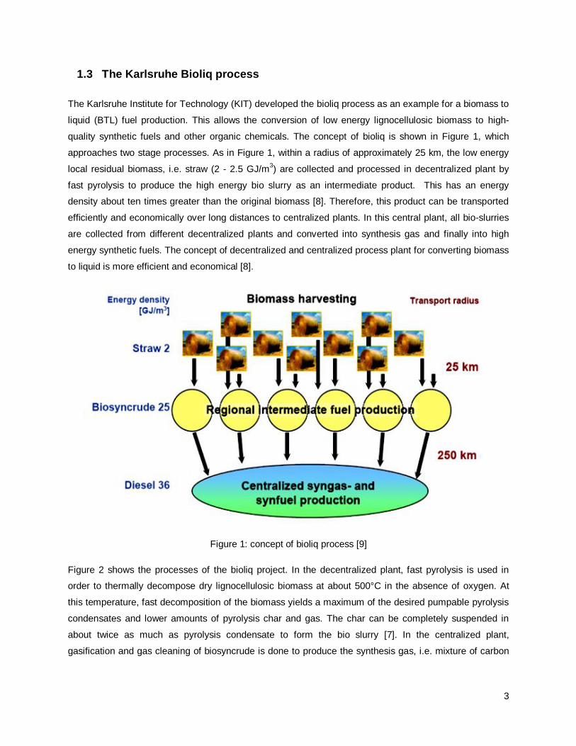
quality synthetic fuels and other organic chemicals. The concept of bioliq is shown in Figure 1, which
approaches two stage processes. As in Figure 1, within a radius of approximately 25 km, the low energy
local residual biomass, i.e. straw (2 - 2.5 GJ/m3) are collected and processed in decentralized plant by
fast pyrolysis to produce the high energy bio slurry as an intermediate product. This has an energy
density about ten times greater than the original biomass [8]. Therefore, this product can be transported
efficiently and economically over long distances to centralized plants. In this central plant, all bio-slurries
are collected from different decentralized plants and converted into synthesis gas and finally into high
energy synthetic fuels. The concept of decentralized and centralized process plant for converting biomass
to liquid is more efficient and economical [8].
Figure 1: concept of bioliq process [9]
Figure 2 shows the processes of the bioliq project. In the decentralized plant, fast pyrolysis is used in
order to thermally decompose dry lignocellulosic biomass at about 500°C in the absence of oxygen. At
this temperature, fast decomposition of the biomass yields a maximum of the desired pumpable pyrolysis
condensates and lower amounts of pyrolysis char and gas. The char can be completely suspended in
about twice as much as pyrolysis condensate to form the bio slurry [7]. In the centralized plant,
gasification and gas cleaning of biosyncrude is done to produce the synthesis gas, i.e. mixture of carbon

4
monoxide (CO) and hydrogen (H2). Finally the synthesis gas is converted into different fuels or other
chemical products, like waxes, methanol, etc. by DME or FT synthesis process.
Figure 2: Process stages of bioliq process [10]
Fast Pyrolysis and Bio slurry production
Firstly, the bio condensate and the bio char are generated from the biomass by fast pyrolysis. Regarding
the operating parameters of the reactor and the used biomass, 50-70% of condensates and 15-30%
pyrolysis char and about 15- 20% gas are obtained. Thus, the main objective of the fast pyrolysis is the
production of adequate organic and aqueous liquid for complete char suspension [9]. Fast pyrolysis is
conducted in a twin screw mixer reactor heated by a sand heat carrier. In the reactor, biomass are rapidly
heated up to approximately 5000C and thermally decomposed within seconds. Central parts of the fast
pyrolysis system are a reactor with twin screws rotating in the same direction, cleaning each other with
looping flights and a heat carrier loop. Technically, a pneumatic sand lift has been applied where the heat
carrier sand is heated directly by means of burned pyrolysis gas which is generated in the process [11].
The fast pyrolysis process is illustrated in Figure 3.

5
Figure 3: Double screw mixing reactor of fast pyrolysis process [12]
Fast pyrolysis of biomass gives a stream of gaseous, vaporized and solid products. The char is separated
from the vapours by a cyclone. The main portion of the vapour is condensed to form liquid pyrolysis
products: organic and aqueous condensate. A single step condenser would result in a condensate mixed
with organic and aqueous condensate. These condensates are not stable and tend to separate in an
organic and aqueous phase. Thus the pyrolysis gases are condensed in two stages. In the initial quench
cooler, the organic substances are condensed at a temperature about 1100C and in the second quench
cooler the aqueous condensate is obtained at low temperature of 400C.
The char obtained in the bioliq process is a fine powder with the size distribution of 10 -200 m and high
porosity of 50- 80%. The char can be suspended in the organic condensate and in the aqueous
condensate. Due to higher heating value of organic condensate i.e. about 20 MJ/kg, it can be used
directly into the gasifier. As the heating value of the aqueous condensate is very low i.e. about 4-7 MJ/kg
it is better to add the char in order to obtain the highest as possible before gasification process.
Gasification, gas cleaning and synthesis process
The next step is an entrained flow gasification, where the bioslurry is partly reacted with oxygen at high
pressure up to 80 bar and temperature more than 12000C to form a tar free synthesis gas (H2, CO) [12].
For the entrained flow gasification, the biomass feedstock needs to be converted into a gas, liquid, slurry

6
or paste, which can be pumped by a compressor pump into the pressurized chamber. Organic fuel with a
higher heating value greater than 10 MJ/Kg can be pumped and atomized in a special nozzle with
pressurized oxygen as gasification and atomization agent[10].
Then the crude synthesis gas is purified and conditioned. The gas purification unit removes precipitate
particles by means of ceramic filter candles, removes acid gas components and alkalis by means of
inorganic adsorbents and catalytically converts NH3, HCN and organic components in a final catalyst
stage. At the last stage of the purification process, CO2 is removed from synthetic gas by a conventional
solvent wash. After purification, the gas converted directly to the DME in a single step synthesis. Then it
proceeds to zeolite catalyzed dehydration of DME with oligomerization and isomerization of the
hydrocarbon used.
The overall characteristics of bioliq pilot plant are illustrated in Table 1:
Table 1: characteristics of bioliq pilot plant [12]
Stage 1 Stage 2 Stage 3 Stage 4 Stage 5
Process Fast pyrolysis Entrained flow
gasification Gas
purification DME
synthesis Gasoline synthesis
Pressure (BAR)
– 80 80 50 55
Temperature (°C)
500 > 1200 500 250 300
Throughput 500 kg/h of
biomass 1000 kg of biosyncrude 700 Nm3/h 50 kg/h 30 kg/h
Product Biosyncrude Crude synthesis gas Pure
synthesis gas DME Gasoline
C5H5.4O1.1 + H2O+ ash
CO+ H2+ CO2 + N2+(H2O)g + slag
CO+ H2+N2

7
2. Literature review
2.1 Biomass and pyrolysis process
2.1.1 Biomass
Biomass is described as “the biodegradable fraction of products, waste and residues from the biological
origin from agriculture (including plants and animal), as well as the biodegradable fraction of industrial
and municipal waste” [13]. By using various conversion processes such as combustion, gasification,
pyrolysis and liquefaction, biomass can be converted into liquid fuels for transportation.
In the pyrolysis process, lignocellulosic biomass consider as a suitable feed stock. The primary
components of lignocellulosic biomass are cellulose, hemi-cellulose and lignin, along with the other
compounds like acids, salts and minerals in lower amounts [14]. The composition of these components
varies depending on the plants. The Table 2 shows the composition of the different lignocellulosic
biomass. For example, hardwood contents higher amounts of cellulose, whereas wheat straw has more
hemi-cellulose.
Table 2: Composition of lignocellulosic biomass [15]
Lignocellulosic biomass Cellulose (%) Hemi-cellulose (%) Lignin (%)
Hardwood 40-55 24-40 18-25
Softwood 45-50 25-35 25-35
Wheat straw 30 50 15
Cellulose is the important component of lignocellulosic biomass, which is considered as a polymer of
glucose. At the temperature between 320-4200C, the cellulose is transformed into organic condensable
vapours, char and non-condensable gases [16]. The cellulose yielded the highest amount of organic
condensate, and low amount of water and char [17].
Hemi-cellulose is a mixture of various polysaccharides such as glucose, galactose, xylose, mannose and
galacturonic acid residues. These components are decomposed at a lower temperature, i.e between 200-
2600C [18]. Thus, under higher pyrolysis temperature significant secondary cracking of pyrolysis vapours
will ocurrs, which result in higher yields of condensate (with higher amount of water content and less tar),
and gas products, and lower amount of char [17], [18].
Lignin is a mostly aromatic polymer consisted mainly of amino acids. It is generally bound to adjacent
cellulose and hemi-cellulose fibers to form a lignocellulosic structure. Lignin decompose between the
temperature range of 280-5000C [18]. The pyrolysis of lignin yield higher amount of char particles,

8
moderate range of condensate (with average percent of organic and aqueous fraction), and lower amount
of gas product [17], [18].
2.1.2 Energy density of biomass
Utilization of biomass as an energy source has several advantages. But due to some properties, the
conversion of biomass into fuel or energy is limited. The energy density of biomass is minimal compared
to that of fossil fuels. Furthermore, biomass contain significant amounts of moisture, up to 40-50% by
weight. The low density and high water content of biomass makes transportation cost higher. So, there
are many traditional technologies to increase the biomass density including baling, cubing and palletizing.
In addition, there are different types of thermo chemical process like pyrolysis, liquefaction through which
low energy density biomass converted into higher energy density products. Figure 4 shows the relative
volume of biomass for wood and straw, intermediate pyrolysis products, and the final mixture (bio slurry).
Bio slurry is well suited for energy density storage and transport, resulting in lower transportation costs.
Figure 4: relative volumes of biomass, intermediate products and bio slurry [7]
2.1.3 Yield of fast pyrolysis product
Pyrolysis is the process of thermal decomposition of an organic component in biomass at various
temperatures in the absence of oxygen, which results in the production of char and non-condensable gas
in slow pyrolysis and additionally condensable vapours (liquid products) in fast pyrolysis.

9
In the fast or flash pyrolysis process, biomass feedstock is rapidly heated to 450 - 600°C in the absence
of oxygen. Under these conditions, vapours, pyrolysis gases and charcoal are produced. The vapours are
quickly condensed to pyrolysis condensates, which tend to separate into a bio-oil (organic condensate)
and reaction water (aqueous condensate). Typically, 60-75 wt. % of the feedstock is converted to
condensates. The product yields of the fast pyrolysis of different biomasses as a reference can be seen in
Figure 5. The products char, organic condensate, reaction water, gas is given on a moisture- and ash-
free basis.
Figure 5: Product yields of different types of biomass [19]
As the organic condensate provides a considerable heating value of about 20 MJ/kg, they can be directly
used in gasification. During a fast pyrolysis of straw, around 65 wt. % of char and condensate are
produced, which can be mixed to form the bio slurry suspension, whereas woody biomass produces up to
80 wt. % with a much higher condensate to char ratio [19].
2.2 Slurry mixing technology
To produce slurries, finely ground char, biomass or coal particles are suspended into organic (bio oil) or
aqueous liquids. These technologies are designed to improve the transportability of the pyrolysis products
and increase energy density, as char or coal powders have low densities due to high porosity. Important
slurry characteristics are the stability, pumpability, atomizability and combustion characteristics [20].
Particle concentration and the particle size distribution are considered as important hydraulic variables in

10
the slurry preparation [21]. Typical slurry production involves preparation, storage, transportation and end
user applications, which is in this case the entrained flow gasifier.
If the pyrolysis products are examined individually, the bio oil may need to be further upgraded and
refined for the production of liquid transport fuels Depending on the water content, the pyrolysis
condensates have a high volumetric energy density and are favourable for transport [22]. The bio char is
also a quality energy carrier, which can be used for co-firing in coal fired plant due to its good grindability
and the significant specific energy densification. But due to the possibility of spontaneous combustion,
long time storage is not favourable. The energy density and therefore the transportability are enhanced by
suspending the bio char in the bio oil respectively the aqueous condensates to produce bio slurry as
energy carrier.
As the particles have a higher density, they might settle down. Hence, it is important that the slurries in
storage tanks remain with uniform solids concentration, or at least remain pumpable while being stored.
Loosely packed sediments are suitable, as long as they can be re-suspended by agitation.
Pyrolysis chars have a high porosity between about 50 to 80%. So during the mixing, the pores first soak
up much liquid until a sufficient volume remains as lubricant outside the particles as showed in Figure 6.
The liquid to solid (L/S) volume ratio, i.e. corresponds to condensate-to-char weight ratio should be 2 to
3:1, which is usually sufficient to prepare free flowing slurries after warming and colloid mixing. If the char
concentration exceeds the sedimentation density as an L/S weight ratio below about 2, pastes or sludge
are obtained. Pumpable slurries of nonporous coal and water with L/S weight ratio of about 0.4 have been
in practice [10].
Figure 6: principle of slurry preparation [10]
Abdullah, Mourant, Li and Wu [23] present fuel and rheological properties of bio slurries, made with bio
oils and pyrolysis chars. They found that the bio slurry has a high volumetric energy densification and
11
meets the requirements for the combustion and gasification process. Thus, this bioslurry can potentially
replace the conventional fuel use in energy plants, or particularly applications like boilers and gasifier.
Natarjan and Suppes [24] investigated the effects of concentration of corn starch on slurry stability,
rheology and viscosity. The mixture with 40% corn starch and 0.15% polyacrylic has favourable
rheological property (i.e. lower viscosity at high shear stress) for injection and pumping and also for slurry
stability. The settling of corn starch particles didn’t occur over a 2 month period.
Benter, Gilmour and Arnoux [25] studied the production of slurries from ground biomass with diesel and
kerosene. They concluded that the settling of wood particles can be stopped by emulsifying the slurry
mixture with the polar liquid like water and/or ethanol. The slurry of 20% ground wood in kerosene with
adding water and ethanol from 15 to 20% produce stable suspension for more than 30 days without any
additional additives. They conducted an experiment with various additives in which addition of rheocin is
found a more suitable stabilizer for enhancing the stability of the slurry mixture.
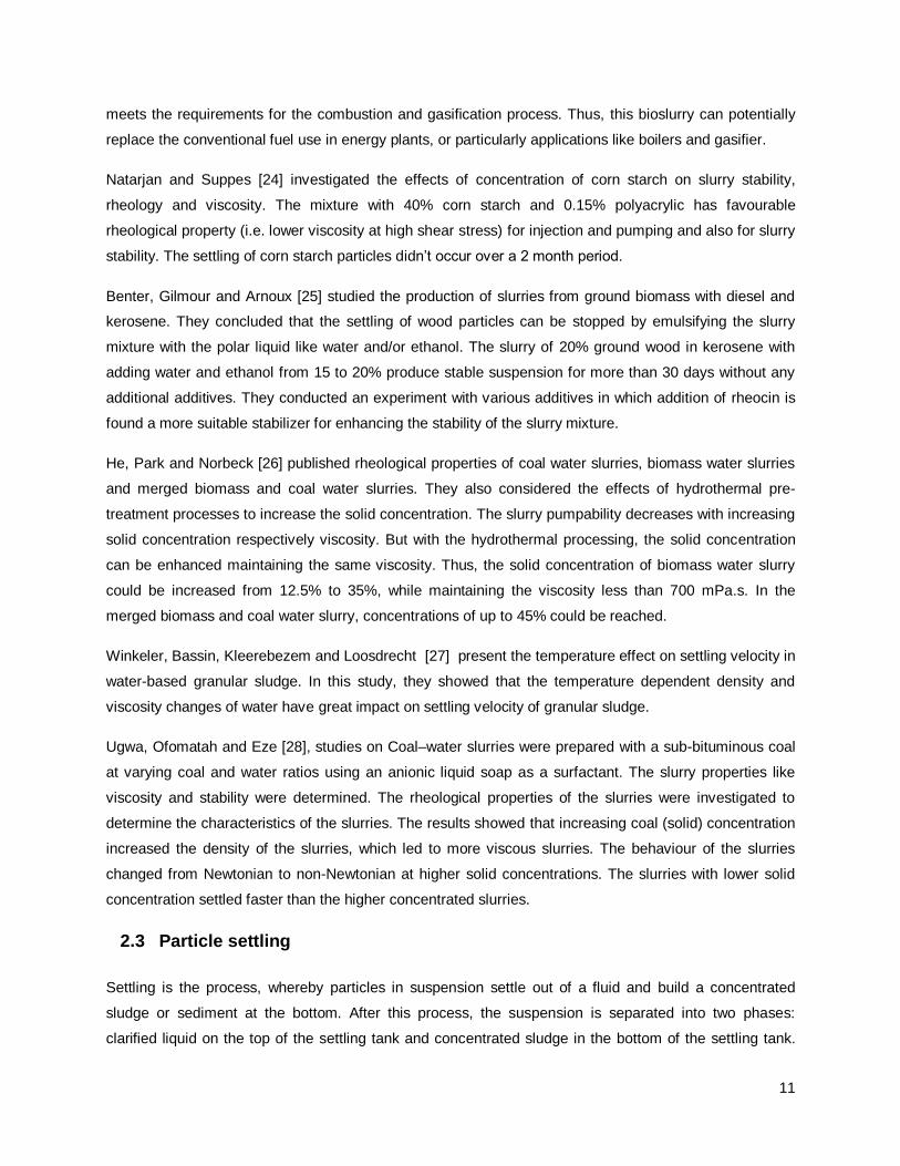
He, Park and Norbeck [26] published rheological properties of coal water slurries, biomass water slurries
and merged biomass and coal water slurries. They also considered the effects of hydrothermal pre-
treatment processes to increase the solid concentration. The slurry pumpability decreases with increasing
solid concentration respectively viscosity. But with the hydrothermal processing, the solid concentration
can be enhanced maintaining the same viscosity. Thus, the solid concentration of biomass water slurry
could be increased from 12.5% to 35%, while maintaining the viscosity less than 700 mPa.s. In the
merged biomass and coal water slurry, concentrations of up to 45% could be reached.
Winkeler, Bassin, Kleerebezem and Loosdrecht [27] present the temperature effect on settling velocity in
water-based granular sludge. In this study, they showed that the temperature dependent density and
viscosity changes of water have great impact on settling velocity of granular sludge.
Ugwa, Ofomatah and Eze [28], studies on Coal–water slurries were prepared with a sub-bituminous coal
at varying coal and water ratios using an anionic liquid soap as a surfactant. The slurry properties like
viscosity and stability were determined. The rheological properties of the slurries were investigated to
determine the characteristics of the slurries. The results showed that increasing coal (solid) concentration
increased the density of the slurries, which led to more viscous slurries. The behaviour of the slurries
changed from Newtonian to non-Newtonian at higher solid concentrations. The slurries with lower solid
concentration settled faster than the higher concentrated slurries.
2.3 Particle settling
Settling is the process, whereby particles in suspension settle out of a fluid and build a concentrated
sludge or sediment at the bottom. After this process, the suspension is separated into two phases:
clarified liquid on the top of the settling tank and concentrated sludge in the bottom of the settling tank.

12
This is natural, when the dispersed particles have a specific gravity greater than that of dispersing
medium: the particles tend to settle down by gravity or centrifugal motion in the direction exerted by that
force. The stability of the suspension depends on the densities of dispersed particle and dispersion
medium, the viscosity of the medium, surface properties of particles and other parameters.
2.3.1 Type of settling
For the low concentration slurry, settling takes place freely following the Stokes equation [29], as in
equation 1. But for the concentrated slurry, the settling becomes a complex process. Also interactions
between the particles form flocs or coagula. So, according to the particles present in the suspension, the
settling can be defined as; discrete, flocculent, hindered settling, or compressive settling.
Discrete or free particle settling:
The particles do not interact with adjacent particles and they settle separately in a gravitational field. In
this type of settling, coarse particles settle at the bottom, whereas the finest particles remain on the top, if
the gravitational forces are not strong enough to overcome frictional forces.
Flocculent Particles Settling:
Individual particles stick together and form loose, porous clumps called flocs. This takes place, when
there is a higher solid concentration and/or chemical reaction influences the particle surfaces to enhance
attachments. The flocs settle relatively slow due to additional drag forces which formed from these flocs,
filling a large fraction of the original slurry volume. Also the loose structure of the flocs contains a
considerable amount of entrapped liquid, leading to a relatively lower density difference. Thus, the volume
of the final sediment is relatively large and it can be re-dispersed by mechanical agitation. Further
compaction of the flocs is only possible by the breaking of the floc bonds and the squeezing out of the
liquid through the surrounding particles.
Hindered particle Settling:
If the concentration of particles in a suspension is increased, individual particles stick together and form a
compact and tightly bound cluster known as coagulated. These clusters tend to settle as a unit and there
is also a net upward flow of liquid, which is displaced by the settling clusters, which leads again to a lower
settling velocity. Formed sediments might be compact and difficult to re-disperse or break. In these types
of settling, it is possible to make a distinction between various distinct zones, divided by concentration
discontinuities. So this is termed as “zone settling“ (see also section 2.4.).

13
Compression settling:
With the highest particle concentration, the settling can occur through compaction of the structure, and so
it takes place at a reducing rate. This is termed compression settling. If the compression settling takes
place, settled particles are compressed under the weight of overlying particles, the pore spaces are
gradually decreased and liquid is driven out of the pores.
2.3.2 Settling velocity equations
The settling can be seen as differential motion among particles of different size, density with relative to
the medium. During this process, flocculation or hindered settling can occur. This is due to complex
interactions between particles and fluid, whose separation is based on the settling rates of particles. For
this, an equation for velocities of falling particles in a liquid suspension is required for different size of
particles. In a free settling, this is comparatively simple to determine, using Stokes or Newton’s law
depending upon the Reynolds number.
Particle settling is controlled by three external forces: gravity force due to the gravitational field, buoyancy
force due to the displacement of the fluid by the particle and the friction force due to relative motion of the
particle and the fluid [30]. These forces are a function of particle properties like size, shape, density and
fluid properties like density and viscosity. As a function of the settling time, the forces reach an equilibrium
point in which the gravity force is balanced by buoyant force and drag forces. From this point, the
particles move at a constant maximum velocity; this is known as settling velocity.
The settling rate in higher concentration systems is influenced by particle collisions, hydrodynamic
interaction and any forces which may reside on the surface of the particle [31]. The higher concentration
of particles in suspension caused the hindered type of settling and the settling rate is defined as the
hindered settling velocity. The hindered settling velocity is the strong function of concentration. Different
models have been developed to established relationship between hindered settling velocity of suspension
and concentration of suspended particles (Richardson and Zaki [32], Concha and Almendra [33]).
Particle settling according to Stokes law
Particle settling velocity of spherical particles for a free settling is given by;
Equation 1
where, Vs is the settling velocity, g is gravitational acceleration, d is the particle diameter, p is particle
density f is the fluid density and the dynamic viscosity [30]. This equation implies for the region where
the particle Reynolds number (RP) is less than 1.

14
Equation 2
Where is the kinematic viscosity.
For the higher Rp, empirical solution is necessary to calculate the drag forces. One such solution is given
by Schiller and Nauman which is valid for Rp< 800 [30].
Equation 3
Hindered settling velocity of a particle
To correlate the hindered settling rate of the suspension with the volume fraction of solids (C) Richardson
and Zaki’s provide hindered settling correlation [32], given by :
Equation 4
Where, V is the sedimentation velocity of the suspension, Vs is the settling velocity of the single particle
and n is the exponent empirically related to the particle Reynolds number (RP). Volume fraction of solids
(C) is equal to volume of particles by the total volume of suspension.
The sedimentation velocity of the suspension is the difference between the settling velocities of particles
and the liquid rise velocity relative to the particle settling. This is given by:
Equation 5
The different relation is given for index n according to the particle Reynolds number:
Equation 6
Equation 7
Equation 8
Equation 9
Where, d/D is the particle to cylinder diameter ratio. For Reynolds number in the Stokes flow region and
negligible wall affect the value of n is given as 4.65 for spherical particles. The parameter n is a function
of Reynolds number, but not a function of particle to wall diameter ratio. By Khan and Richardson
proposed relation of n relates to the Archimedes number (Ar) given by[34]:

15
Equation 10
Where, Ar is given by:
Equation 11
Wallis suggested determining the index n by the approximation[35].
Equation 12
Which cover all range of Rp
2.3.3 Method for sedimentation analysis
Based on different combinations of the force field, the level of measurement in the suspension and the
dispersion of particles at the start of the measurement, there are different methods for sedimentation
analysis. According to the position of particles at the beginning of the measurement, there are
“homogeneous methods”, where particles are uniformly distributed and “line start methods” where
particles at the beginning are concentrated in a thin layer up the top of the solid free medium. Depending
on the place of quantity measurement in the suspension, there is the “incremental method”, where the
concentration of solids in a thin suspension layer is measured in knowing height and time. With the
“cumulative method”, the rate of solids settle out of suspension is measured. There are measurements
based on particle mass, such as the sedimentation balance method, decanting method and pipette
method; measurement based on suspension density, such as the method using manometers, aerometer
or various divers and measurements based on the electromagnetic radiation such as light attenuation,
scattering of -radiation, of light or x-rays and backscattering of -radiation [36] [37].
Li, Lou and Qiu [38] studied the stability of coal water slurry and sedimentation behavior of particles with
the dispersion stability analyzer and concluded that the analyzer provides more accurate data than
traditional methods. This analyzer provides more applications like to analyse the stability of the slurry with
observing the stability mechanism of slurries.
2.4 Batch sedimentation or zone settling
If there is no adding or remove of the slurry during the sedimentation, the process is called batch
sedimentation, whereas, if the solids are steadily removed, the process is called continuous thickening.
In batch processing, initially the sedimentation tower contains a homogenous mixture. Figure 7
represents a typical batch settling column test on a suspension showing zone settling characteristics. As
the settling takes place, at the top of the tower a clear liquid interface is formed (A). As the particles settle

16
down, a uniform concentration zone (B) and a non-uniform zone (C) is formed. At the bottom, solid
particle compressed and formed stronger sediment (D) with the increasing storage time.
Figure 7: Zone settling behaviour in typical batch sedimentation [39]
A: clear liquid, B: uniform mixture, C: non uniform mixture, D: sediment
t:time, x: suspension height, x”: interface height at certain time, x’: final interface height at dt
In Figure 7, initially, the suspension settles at a constant rate in the section A to B, and if the particles
become of fairly uniform size, sharp discontinuities form between these layers. Between the regions B
and C there may or may not be distinct continuity. As the time increases, the upper discontinuity meets
the lower and the region B disappears. Then a gradual compression of the regions C and D occurs until
finally the sediment formed. The slope of the settling curve at any point represents the settling velocity of
the interface between the suspension and the clear liquid.
Since there is no net flow through the tower, the continuity equation is given by:
Equation 13
Where, Qp is the volume flow rate of particle settling is given by:
and Ql is the volume flow rate of liquid moving upwards is given by:
Thus the velocity of liquid can be calculated by:
Equation 14
This type of settling has been analyzed by Kynch (1952) [39]. His analysis is based on the assumptions
that the settling velocity of particles Vc is a function only of the local concentration (C) of particles and the
settling velocity tends to decrease as the concentration approaches a limiting value corresponding to that
of the sediment layer deposited at the bottom of the settling column.
B
A
B
D
C C
D
A
D
A
Height
Time
X’
X”
dt

17
The volumetric rate of sedimentation per unit area or flux (J) is given by:
Equation 15
Two layers at height x and x+dx within the transition zone are considered as shown in Figure 8, having a
suspension concentration C. On its upper layer, there is a layer of lesser concentration and on its lower
layer there will be a layer of higher concentration. By the time dt the position of this layer moves upward
with the rate of u and settling rate of particles decrease by dVc.
Figure 8: Kynch settling behaviour
Since the concentration within the layer between x and x+dx remains constant, the influx of particles
through the upper layer must be equal to the out flux of particles through the lower layer.
We get,
Equation 16
Since Vc is a function of C and assume as constant, thus the rate of rising of any plane of fixed
concentration is constant i.e. u = constant =dx/dt. In a uniform suspension of concentration C, the
interface between the suspension and the liquid will fall at a constant rate until a zone of composition
greater than C, has propagated from the bottom of the free surface. The sedimentation rate will then fall
off as a zone of higher concentration reaches the surface, until sedimentation will stop when the Cmax
zone reaches the surface.
The relation between Vc and C can be obtained from a batch settling test. In the beginning at time t=0 the
suspension has uniform concentration C and at initial height x. Over time t= t’ the interface has dropped to
a height x” and the new concentration is a C’. The total mass of solid in the column at t=o, is given by
CxA, where A is the cross section area of the column. At time, t=dt the total mass will have to pass
through the plane of concentration C’ as it moved up from the base of the column with velocity u. This is
given by:

18
Equation 17
Thus the velocity of ascent is constant and therefore equal to dx”/dt, we get:
Equation 18
The settling velocity of the particle is given by the slope of the settling curve at (x’, dt) and from Figure 7
by drawing a tangent to the curve at this point the slope is equal to -(x” – x’)/dt . Thus we obtain:
Equation 19
Therefore, in batch settling test the settling velocity for any given concentration can be obtained and the
concentration at the interface can be determined.
2.5 Rheology
Rheology is the survey of the flow of matter; liquid or solid under conditions in which they flow rather than
deform elastically. This also applies to substances with a complex structure like: mud, slurry,
suspensions, and polymer materials. Fluid behaviour is shown in Figure 10. Two extreme of rheological
behaviour are:
Newtonian or Viscous behaviour: any deformation that ceases when the applied force is removed. The
viscosity is constant with changing shear rates, i.e. the relation between the shear stress and shear rate
is linear passing through the origin. Simple Newtonian behaviour is given by;
Equation 20
Non- Newtonian behaviour: viscosity of non Newtonian fluid is dependent of shear rate. The relation
between the shear stress and the shear rate is not linear, i.e. shear stress change with the shear rate.
This type of fluid behaviour is found common in coal water slurry, coal algae slurry, coal oil mixture, coal
biomass slurry, sludge slurry, and bio char slurry [40],[41],[42],[28], [43]
Types of Non- Newtonian behaviour
Time independent viscosity
This type of flow behaviour is not affected by the length of time that the fluid has been flowing.
19
Pseudo-plastic or shear thinning: structures and the viscosity changes with the force. Molecules or
particles are arranged in order pattern. The viscosity of pseudo-plastic fluids decreases with the
increased shear rate as shown in Figure 10.
Dilatant or shear thickening: resists distortion more than in proportion to the applied force. Molecules or
particles are arranged in disordered pattern. For dilatant fluids, the viscosity increases with increased in
share rate as shown in Figure 10.
Time dependent viscosity
When viscosity at a given shear depends on time, the systems are;
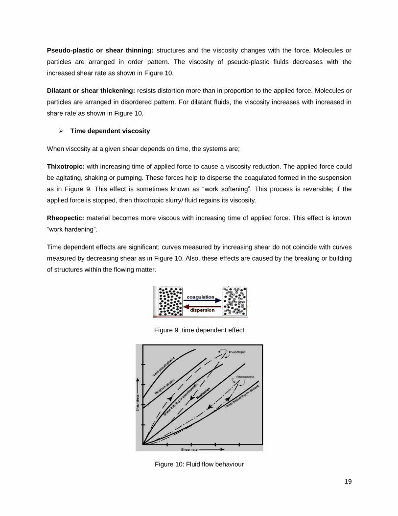
Thixotropic: with increasing time of applied force to cause a viscosity reduction. The applied force could
be agitating, shaking or pumping. These forces help to disperse the coagulated formed in the suspension
as in Figure 9. This effect is sometimes known as “work softening”. This process is reversible; if the
applied force is stopped, then thixotropic slurry/ fluid regains its viscosity.
Rheopectic: material becomes more viscous with increasing time of applied force. This effect is known
“work hardening”.
Time dependent effects are significant; curves measured by increasing shear do not coincide with curves
measured by decreasing shear as in Figure 10. Also, these effects are caused by the breaking or building
of structures within the flowing matter.
Figure 9: time dependent effect
Figure 10: Fluid flow behaviour

20
3. Materials and Methods
3.1 Materials and its properties
3.1.1 Char
As for the theoretic study of this work, the unmilled straw char from the fast pyrolysis step of the bioliq
process was used. The char sample was taken in December 2013 from the bioliq plant. Due to fluctuation
in pyrolysis parameters in the bioliq plant, the char properties are not very constant. Table 3 shows the
average properties of the char used for the bio slurry.
Table 3: properties of Char
C (%) 54.3
H (%) 1.9
N (%) 0.4
Ash content (%) 35.8
Bulk Density (kg/m3) 250
Calorific value (MJ/kg) 20.5
The straw char contains 54.3% carbon and has also a high ash content of 35.8%. The straw char has a
low bulk density of 250 kg/m3 due to the formation of agglomerates having interspaces between the
individual particles, as well as intra-particle pores. The straw char contains a high porosity of 50-80%,
which strongly influences the slurry preparation because initially the liquid is drawn by capillary forces in
the pores or interspaces of agglomerates, and so a significant part of the liquid is immobilized.
3.1.2 Aqueous condensate
The aqueous condensate from the bioliq plant was used for the preparation of the bio slurry. The
pyrolysis condensates are less stable and have a tendency to separate in two phases. In the bioliq plant
the pyrolysis vapours are condensed in two steps for obtaining an aqueous condensate and an organic
condensate. The organic condensate has a high heating value of about 20 MJ/kg, so it is used directly in
the gasification process. For the aqueous condensate, the heating value is about 4-7 MJ/kg, which is too
low for the direct gasification. By mixing the aqueous condensate with the char the higher heating value of
the mixture increase and be suitable for the gasification and.
Table 4 shows some properties of the used aqueous condensates. The organic compounds in the
aqueous condensates are mainly acids, leading to a pH of 2.65.

21
Table 4: Properties of aqueous condensate
3.1.3 Bio slurry
Bio slurry is a suspension of pyrolysis condensates and pyrolysis char. In this study, the bio slurry was
prepared by mixing the aqueous condensate and the char in a colloidal mixer from MAT Company. In this
mixer, the shear rate is high enough to completely destroy the solid char agglomerations.
For the present study, the bio slurry with three different concentrations were prepared. At first, one ton of
the bio slurry mixture was prepared in the beginning and is stored in an IBC. The concentration result is
discussed in section 4.1. Due to the particle settling the mixture becomes non-homogenous after an hour.
So to maintain the mixture homogenous, a motor is used to stir the bio slurry continuously at around the
speed of 800 to 1000 rpm. This first prepared bio slurry named as “alpha” and used for the alpha slurry
experiment.
The second bio slurry with higher concentration was prepared by adding the slurry from alpha slurry
experiments and the prepared slurry named as “beta”. To increase the concentration slurry separated
aqueous condensate in the alpha slurry experiment was removed and remaining higher concentrated
slurry was added in the remaining alpha bio slurry in the IBC and then this mixture was stirred
continuously at the same speed. The third bio slurry with higher concentration was prepared by adding
the higher concentrated slurry from beta slurry experiments and the prepared slurry named as “theta”.
3.2 Experimental setup
For characterizing the particle settling of bio slurry the experiments were done in a two different scales.
3.2.1 Big scale tower
In a big scale experiment, a tower with 150 cm in height, 55 cm in breadth and 55 cm in width, which has
a capacity of 450 L, was used. To sample the slurry, 25 outlets were fixed at the front side of the tower as
shown in Figure 11. The distances between two outlets were 6 cm. The bio slurry was filled from the top
of the tower and covered with a plate to avoid evaporation. After the defined settling time as in section
Water content (%) 84.8
pH 2.65
Mass density (kg/m3) 1020
HHV (MJ/kg) 4-7

22
3.3, slurry samples were gathered from each outlet to measure the solid concentration by filtration. By
removing the front plate, the tower was emptied and cleaned, and refilled with a new slurry of a different
(higher) concentration. In the results, a first outlet at the top is considered as the outlet number 1 and
followed to the last outlet as outlet number 25 at the bottom as shown in Figure 11.
Figure 11: front side of tower with outlets (a tower with 150 cm, 55 cm and 55 cm in height, breadth and
width respectively, and 25 outlets at a distance of 6 cm between two outlets)
3.2.2 Small scale cylinder
For the small scale experiment, cylinders with a vertical height of 20 cm were made out of 5 segments
and the bottom side is closed with a cover. Each segment has a diameter of 5 cm and a height of 4 cm.
At first, two segments are joined together with tape. To increase the height of the cylinder another
segment is kept in top of the fixed segments and joined with the tape. Similar process followed till the
desired height obtained. For the experiments, five segments were joined together with tape to make a
small settling cylinder. The resulting sedimentation tower is shown in Figure 12.
1
25
4
7
10
13
16
19
22
2
5
8
23
20
17
14
11
3
6
9
12
15
18
21
24

23
Figure 12: small scale sedimentation tower (tower height of 20 cm)
3.3 Experimental strategy
For the study of the particle settling of the bio char particles in the bio slurry, the sedimentation method
was used. In the sedimentation method, the bio slurry is allowed to settle in a sedimentation tower for a
set period of time. The measurement of the char concentration at different levels of the tower was
determined at different time intervals of 4 hours, 8 hours, 1 day, 3 days, 7 days and 14 days. To find out
the influence of the char concentration in the slurry, experiments were carried out with three different
concentrated slurries. The slurry names are given as “alpha”,”beta” and”theta” and the properties of these
slurries are discussed in section 4.1. With the beta slurry, experiments were done to find out the influence
of the height for the particle settling in the slurry mixture. For this study, one experiment was carried out
with the beta slurry in big tower filled full level (150 cm) and around half level (84 cm) and also in the
small scale cylinder with (20 cm).
To find out the influences of the temperature in the settling of the particles in the slurry mixture, the
experiment was performed in different temperatures, i.e. room temperatures, i.e. 2020C (TR), 35
0C (T35)
and 450C (T45) in a small scale tower with the beta slurry. In the big scale tower, the experiment was
done only at room temperature.
3.4 Experimental procedure for measuring the solid concentration distribution
The measurement of char concentration in the sample slurry was made by separating the char particles
by filtration followed by washing the ethanol and evaporation of the liquid components.
3.3.1 Big scale tower
In a big scale tower, the slurry was taken out from each outlet and measured the weight of the sample. As
the char particle is porous, it soaked the condensate and formed clusters of very low volatility. Therefore

24
the sample slurry is diluted with ethanol and stirred for around 20-30 seconds for proper mixing before
filtration. Thus porous particles and the gaps between the particles are filled with ethanol and due to the
low boiling temperature of ethanol it dried easily. Then the sample is filtered as in Figure 13 to collect
char particles. After the filtration, the char is dried in the oven for minimum 6 hours at around 1000 C to
evaporate all the ethanol and condensate from the char particles. At last, the solid weight of char from
each outlet was measured. By this method, we distinguished the phase separation zone and a solid
concentration in different time intervals.
Figure 13: filtration of sample bio slurry
3.3.2 Small scale tower
For the measurements of the small scale tower, the towers were filled with slurries and allowed to settle
for the defined sedimentation interval. Then the tape was cut stepwise from top of the column down. At
first, the sample tower was kept in the beaker and the tape between the first segment and second
segment was cut with the knife. So that the suspension coming out from the cutting portion is collected in
the beaker. Slowly the first segment with sample was drawn out from the settling tower and kept in the
beaker. Sequently with the same procedure the second, third, fourth and fifth segments were drawn out
and kept in the different beaker as in Figure 14. The weights of the each beaker with the slurry sample
and segment were measured. Then the slurry sample was diluted with ethanol to separate the
condensate from the char particles. Then the mixtures were filtered and after a while kept in the oven for
the drying for minimum 6 hours at around 1000 C to evaporate all the ethanol and condensate from the
char particles. The weight of the each beaker and the segment was measured. Thus, by subtracting the
weight of the beaker and segment, the weight of slurry sample was calculated for each segment. After
drying, the mass of the dried char particles from each segment was measured. With these results the
phase separation and the particle settling within the slurries was distinguished.

25
Figure 14: sample slurries from different segments
3.3.3 Influence of temperature
To find out the influences of the temperature in the settling of the particles in the slurry mixture, the
experiment was performed in different temperatures, i.e. 200C (TR), 35
0C (T35) and 45
0C (T45) in a small
scale tower with the beta slurry. The experiments at the 200C were carried out in the room temperature
with 20C. While for the higher temperature at 35
0C and 45
0C, the settling tower was kept in the oven as
in Figure 15 till the defined settling time of 4 hours, 8 hours, 1 day, 3 days, and 7 days at the constant
temperature. After the defined time, the measurement of solid concentration on each segment was
followed by the same process as defined in section 3.3.2,.
Figure 15: slurry in oven at constant temperature

26
3.3.4 Static stability test
The stability of a slurry against gravity is called static stability. A statically unstable slurry will settle down
and formed a compact sediment. While with the static stable slurry, the settling rate is less and allow the
slurry flow smoothly. The factors affect the slurry stability are particle size, density, solid concentration,
surface properties. The static stability of the slurry is an essential element in its applicability, which decide
the value of the slurry. The static stability is significant in order for handling of the slurry likely to stirring
requirement or the function of additives to minimize settling.
The calculation of bio slurry stability was carried out with a equation used for the coal water slurry method
[44]. A bio slurry sample was filled in a small scale tower (with 20 cm height) and measures the weight of
slurry sample. Then the slurry was kept in a room temperature for 7 days. After 7 days, the slurry tower,
then was turned upright for 8 minutes to let the slurry flow adequately from the tower. Afterwards, the
mass of the non-flowing parts of the bio slurry was measured. The stability of bio slurry could then be
calculated using the equation:
Equation 21
with Ssta as the static stability (%), MI as the initial mass of the bio slurry sample (g) and MN as the mass
of the non-flowing bioslurry (g).
3.3.5 Settling test in graduate cylinder
The settling of the char particles in aqueous suspension was studied in small batch experiments. A slurry
of known concentration was filled in a graduate cylinder at room temperature as in Figure 16. The
experiment was carried out with different initial settling height of 250 mm, 200 mm, and 150 mm. As the
particle start to settle, the position of the interface between the settled particles and an almost particle
free condensate was noted after a time interval of 30 min. The experiment was stopped when there was
no change in the interface height. Then the height of the interface was plotted versus time. The settling
velocity of the particles Vc in a suspension was determined by measuring the slope of the linear portion of
the height against time.
Figure 16: batch settling in graduate cylinder

27
3.3.6 Viscosity measurement
Viscosity is a measurement of the resistance of fluid or suspension, which is being strained by the shear
stress. The viscosity was measured with the rheometer in the. Rheometer is a device used to measure a
liquid, slurry or suspension flows in response to applied forces. The rheometer are equipped with a
various modular like plate-plate, cone and plate and coaxial cylinder measurement systems under
controlled-stress or controlled-rate conditions.
The viscosity was measured with the rotational rheometer in the analytical lab of IKFT as shown in Figure
17. In this experiment the defined speed (shear rate) between 1 to 100 is applied and the dynamic
viscosity was measured. The slurry sample was loaded into the concentric cylinder system which is
designed to impose simple shear flow when rotated. Then the cylinder was kept in the holder of the
rheometer and tight it with screw. And the spindle is fixed with the coupling just below the mounting. The
mounting can slide up and down. For all measurements, helical spindle was used, due to its high
accuracy of viscosity values and to avoid turbulent rheological regime. The spindle was fixed to the
mounting by the coupling. The spindle was automatically detected by the encoder. This encoder is
connected to computer by electrical wire signals which transform the mechanical action into electrical
signals and show us in a graphical form by software which is “rheoplus”. When we analyze non-
Newtonian fluid like in our case is a slurry of char and aqueous condensate, a plot of viscosity vs. spindle
speed is constructed. Viscosity is plotted along the y-axis and speed (RPM) along the x-axis. The shape
of the curve indicates the type and degree of flow behavior as shown in the Appendix A.
Figure 17: rotational rheometer setup
A: mounting, b: computer, c: spindle d: holder
a
b
c
d

28
4. Result
4.1 Analysis of slurry parameter
4.1.1 Slurry compositions
The analysis of the bio slurries was done by the analytic lab of the IKFT. It measured the concentration of
the char and the water content in the bio slurry. Bioslurry alpha prepared from a colloidal mixture had a
concentration of 23.4% char and 67.6% of water as shown in Table 5. As described in section 3.1.3, by
adding higher char concentration slurry the new slurry “beta” was prepared with a char concentration of
26%. The final bio slurry “theta” has had a char concentration of 31.3%. The pH of all of the three slurries
was 5.7.
Table 5: bio slurry analysis
S.N char % pH H2O %
alpha 23.4 5.7 67.6
beta 26 5.7 65.8
theta 31.3 5.7 65.5
4.1.2 Particle analysis
The size and shape of particles regulate the flow and compression properties. The smaller particles break
up more and result in higher suspension rate than larger particles. Also from the Stoke’s equation, it's
seen the particle size is directly proportional to the settling velocity, thus the larger particles are expected
to settle faster than the small particles, but in the experiments, no different particle size distribution could
be found of the height, which is justified with the high solid concentration and the hindered settling. . The
particle size distributions (PSD) of bio slurry samples are shown in Table 6 and sum distribution and
particle spectrum are illustrated in Appendix A. The particle size distribution X50 of all three slurries was
below 30 m. X95 for the alpha, beta and theta slurry is almost 84 m, 80 m, and 70 m respectively.
The mean sizes of the particles in the alpha, beta, and theta slurry were 40.70.6, 38.80.8, and 36.21.2
m respectively. The decrease can be explained by the stirring treatment in the IBC.
Table 6: particle distribution for different slurries
sample X5 (m) X50 (m) X95 (m) Mean (m)
alpha 6.32 28.98 83.87 40.70.6
beta 5.86 26.81 80.33 38.80.8
theta 5.68 26.10 70.74 36.21.2

29
4.1.3 Viscosity analysis
The viscosity is a significant parameter to characterize the slurries. The viscosity of the slurry is
influenced by several parameters like temperature, particle size, particle concentration and the viscosity
of the liquid medium. The viscosity was measured as a function of shear rate and temperature as
illustrated in Figure 18 and Figure 19 respectively. Figure 18 describes that the characteristics of the
slurries at 200C generally present non-Newtonian behaviour. The viscosity of the slurry varied as the
shear rate was changed. Pseudo-plastic or shear thinning behaviour is characterized by the decrease in
viscosity as the shear rate increases. A similar trend was found at higher temperature (i.e. 350C and
500C). The data for viscosity analysis are presented in Appendix A. It should be mentioned that the
viscosity strongly decreases with increasing shear speed. Higher shear rates likely letting out the
interactions and the closeness of particles thereby reducing viscosity. In this case, values with the
analytically lowest possible shear speed of 1 rpm can be measure with the rotary rheometer.
As expected viscosity increases with the increase in particle concentration. Theta slurry with 31%
concentration had a higher viscosity than the alpha and beta slurries with concentrations of 23% and 26%
respectively. The viscosity increases because of the frictional forces between the particles become
significant, and also the blockage of free condensate occur. Thus, the lubrication effect of free-flowing
condensates are become ineffective [45].
Figure 19 shows the viscosity as a function of the temperature for different slurries at 50 rpm. As
expected the viscosity of the slurry decreased as the temperature increased. This is because of cohesive
forces between the particles decrease with the increasing temperature. Thus, the forces of attraction
between particles decreases, which reduces the viscosity of the slurry. The viscosity at different shear
rates are presented in Appendix A, which shows a similar trend as in Figure 19.

30
Figure 18: viscosity of slurry as a function of the shear rate at 200C
(theta:31.3%, beta: 26%, alpha:23.4%)
Figure 19: viscosity as the function of temperature
(theta:31.3%, beta: 26%, alpha:23.4%)
100
1000
10000
100000
0 20 40 60 80
vis
cosity (m
Pa.s
)
Shear rate (rpm)
Slurry
theta
beta
alpha
0
500
1000
1500
2000
2500
3000
3500
20 35 50
vis
cosity (m
Pa*s
)
temperature (0C)
slurry
theta
beta
alpha

31
4.2 Characterization of sedimentation
In this section, the sedimentation of the bio slurry is characterized according to the influence of the char
concentration, of the height of the column and of the temperature. The complete figure of all experiments
is shown in Appendix B.
4.2.1 Influence of concentration of char
As mentioned in section 3.2, the experiments were done with three different concentrations with slurries
named “alpha”, “beta” and “theta” and the corresponding properties were presented above in section 4.1.
Figure 20 shows the char concentration at different column levels (outlet) at different times in the
experiment with slurry containing 23.4% of char. This experiment was carried out at full tower (i.e. height
of 150 cm). After 24 hours, the phase separations are clearly shown in Figure 20 at the outlet number 6
(i.e. height of about 30 cm from top). In the top 5 outlets, the char concentration fell below 5%, whereas
from the outlet number 7 to the outlet number 25 the char concentration increased to a maximum of 27%.
In between outlet number 5 and 6, the particles fell slowly and after 336 hours the concentration on this
level became nearly zero. After 72 hours, the concentration in the outlet number 7 tends to decrease
steeply. Whereas, from the outlet number 8 to the outlet number 25, the slurry concentration remains
nearly same till 336 hours. The maximum concentration goes to 29% on outlet number 25 on day 14.
Figure 20: concentration measurement at different time intervals for alpha slurry
Figure 21 shows the char concentration at a different level in the tower at different time intervals for the
“beta” slurry. In the beginning, the char concentration in the slurry was 26%. For this experiment, the
0
5
10
15
20
25
30
35
0 24 72 168 336
Concentr
ation(%
)
time (hour)
outlet no.
25 (147 cm)
15 (87 cm)
9 (51 cm)
8 (45 cm)
7 (39 cm)
6 (33 cm)
5 (27 cm)
4 (21cm)
2(9 cm)

32
tower was filled almost half (84 cm) of the filling level of the previous experiment. The influence of the
initial suspension height is presented in section 4.2.2. From outlet number 16 to outlet number 25 the
concentration rises up to 31% from the initial concentration after 4 hours and then increased very slowly
to a maximum of around 33% till 336 hours. Whereas in first two outlets (i.e. height of about 9 cm) the
concentration went down below 5% in 4 hours and tended to zero percent concentration after 8 hours.
After 24 hours, it was possible to obtain an almost clear aqueous phase in the first three outlets (from
outlet number 12 to 14 i.e. height of about 15 cm). After 24 hours, particles settle slowly in between outlet
number 15 and 16 (height of 21 cm to 27 cm). At 336 hours, outlet number 15 became a nearly char free
zone, while the concentration at outlet number 16 goes down to 7%.
Figure 21: concentration measurement at different time intervals for beta slurry
Figure 22 shows the results for the “theta” slurry with a concentration of 31.4%. As for the experiment
with the beta slurry, this experiment was also carried out with the tower half filled. Thus, after 24 hours,
almost all char particles settled down below the height of 15 cm correspondent to the outlet 14. On the
bottom of the tower i.e.outlet 25, the char concentration is almost same to the initial concentration. After
72 hours, there was no significant change in the char concentration in any level of the tank. The
maximum concentration goes to 34% in outlet number 25 after 336 hours.
0
5
10
15
20
25
30
35
0 4 8 24 72 168 336
Concentr
ation(%
)
time (hour)
outlet no.
25 (81 cm)
18 (39 cm)
17 (33 cm)
16 (27 cm)
15 (21 cm)
14 (15 cm)
13 (9 cm)
12 (3 cm)

33
Figure 22: concentration measurement at different time interval for theta slurry
Comparing the results obtained with slurry theta and beta it can be seen that with the higher
concentration of the slurry the lesser the concentration change at the lower level corresponding to the
outlet number 25. In fact, it seems likely that the initial concentration of around 31% is closer to the
maximum packing density. Also, it can be seen that after 24 hours a relative sediment concentration has
formed from outlet number 8 for alpha slurry and outlet number 17 for beta slurry and from outlet number
15 for the theta slurry. After this, the particle settling process becomes slower because the displaced
liquid has to flow through the small spaces between the particles and the resistance to the flow of liquid
progressively increases.
From the above figures, it is also possible to conclude that that the rate of settling of the particles tends
to decrease as the concentration of particles approaches a limiting value corresponding to that of the
sediment layer deposited at the bottom of the tower. With higher concentrations of particles in the
suspension, interactions between the particles increase and limit the movement of the particle relative to
each other.
Comparing the results presented in Figure 21 and Figure 22, it is possible to conclude that the
concentration changes after 24h were lower in the experiment with the theta slurry. In fact, for this slurry
the larger variation obtained was off about 5% in the outlets 15, whereas for the beta slurry, the decrease
of the concentration was off about 15% in the same outlets. At 336 hours, it was observed that, slurry with
an initial concentration of 31.3% (theta slurry), the interface level between the particles and condensate is
up to the height of 15 cm. Whereas, slurry with a lower concentration of about 26% (beta slurry), particles
tend to settle down around the height of up to 21 cm.
0
5
10
15
20
25
30
35
0 24 72 168 336
Concentr
ation(%
)
time (hour)
outlet no.
25 (81 cm)
18 (42 cm)
17 (33 cm)
16 (27 cm)
15 (21 cm)
14 (15 cm)
13 (9 cm)
12 (3 cm)

34
With the Equation 19, the average concentration of the sediments may be calculated from the data in
Table 7 obtained from the experiments. The average concentration was initial concentration times the
initial height by sediment height. The result of average concentration of the sediment was calculated as in
Table 7. This shows that the calculated average concentration is nearly the same concentration obtained
from the experiment.
Table 7: average concentration of sediment
Initial slurry concentration
(%)
Initial height (cm)
Interface height (cm)
Relative interface level
(%)
Sediment height (cm)
Average concentration of sediment (%)
23.4 150 33 22 117 30
26 84 21 25 63 34.7
31.3 84 15 17.9 69 38.01
4.2.2 Influence of settling height
For the study of the influence of the height as described in section 3.3, the big tower was filled full level
(150 cm) and around half level (84 cm) with a beta slurry (26% char content) and experiment was also
carried out in the small scale cylinder (20 cm) with the beta slurry.
Figure 23 shows the settling of char particles as a function of the relative height at different time intervals.
After 8 hours, phase separation was seen at the relative height of 30% in all three initial heights. In
relative height higher than 30% the concentration of the char is increased to maximum packing density.
After 1 day, there was no significant change in the char concentration in all experiments from 40 %
relative heights to end of the tank. After day 3, in the top level, i.e. to 20% relative heights, the char
concentration was almost zero in all three experiments and at the lower level there is no significant
change in the char concentration. After 7 days, the interface level is almost to 20% relative height in all
experiments.
The result clearly shows that, the height of the settling tower did not affect either the settling trend or the
consistence of the sedimentation. From all these figures at different interval of time, there the
concentration of the char particles in different level or relative height is almost same and the solid
concentration in the bottom region was also almost the same. This means that the hydrostatic pressure of
the suspension did not influence the particle settling. Therefore, small scaled experiments can be scaled
up.

35
(a) (b)
(c) (d)
Figure 23: char concentration as a function of the column height (a) after 8 hours, (b) after 1 day, (c) after 3 days, (d) after 7 days
0
5
10
15
20
25
30
35
0 10 20 30 40 50 60 70 80 90 100
Concentr
ation(%
)
Relative Height (%)
150 cm
84 cm
20 cm
0
5
10
15
20
25
30
35
40
0 10 20 30 40 50 60 70 80 90 100
Concentr
ation(%
)
Relative Height (%)
150 cm
84 cm
20 cm
0
5
10
15
20
25
30
35
40
0 10 20 30 40 50 60 70 80 90 100
Concentr
ation(%
)
Relative Height (%)
150 cm
84 cm
20 cm
0
5
10
15
20
25
30
35
40
0 10 20 30 40 50 60 70 80 90 100
Concentr
ation(%
)
Relative Height (%)
150 cm
84 cm
20 cm

36
4.2.3 Influence of temperature
Figure 24 and Figure 25 show the influence of the temperature and time and the sedimentation of char
for the beta slurry. The result shows that the settling of the char at room temperature (2020C) is lower
than at a temperature of 350C and 45
0C. From Figure 24 (b), (c), (d) and (e) it can be seen that the
concentration at a temperature of 350C and 45
0C fell slowly in top segments and slightly increased in the
bottom segments. At room temperature the concentration from the second segment to last segment
seemed constant after 4 hours.
(a) (b)
(c) (d)
0
5
10
15
20
25
30
35
4 8 12 16 20
Concentr
ation (
%)
height (cm)
4 hr
T 20
T 35
T45
0
5
10
15
20
25
30
35
4 8 12 16 20
Concentr
ation (
%)
height (cm)
8 hr
T 20
T 35
T 45
0
5
10
15
20
25
30
35
4 8 12 16 20
Concentr
ation (
%)
height (cm)
1 day
T 20
T 35
T 45
0
5
10
15
20
25
30
35
4 8 12 16 20
Concentr
ation (
%)
height (cm)
3 day
T 20
T 35
T 45

37
(e)
Figure 24: concentration of char as a function of temperature (a) after 4 hours, (b) after 8 hours, (c) after 1 day, (d) after 3 days, (e) after 7 days
Figure 25 shows the previous results, but only for the first segment (height 4 cm) and the last segment
(height 20 cm). Thus, it is clear that the increase of the temperature favours the sedimentation rate
because after 4 hours, at room temperature (2020C) the concentration of char at the top segments goes
down to 14%, while at 350C and 45
0C this concentration is 5% and 4% respectively. In the bottom
segments, the char concentration at room temperature (2020C) and at a temperature 35
0C and 45
0C has
a difference of around 3%. However, for the bottom segment the influence of the temperature is not
important. These results indicate that, in order to avoid the sedimentation of the char particles, it is better
to store the bioslurry at lower temperature.
Figure 25: concentration as a function of temperature for first (top) segment and last (bottom) segment
0
5
10
15
20
25
30
35
4 8 12 16 20 C
oncentr
ation (
%)
height (cm)
7 day
T 20
T 35
T45
0
5
10
15
20
25
30
35
40
0 4 8 24 72 168
concentr
ation (
%)
time (hour)
T 20 top
T 20 bottom
T 35 top
T 35 bottom
T 45 top
T 45 bottom
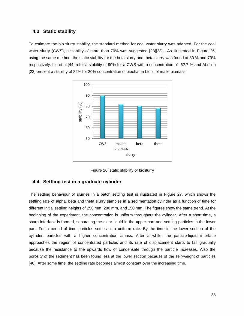
38
4.3 Static stability
To estimate the bio slurry stability, the standard method for coal water slurry was adapted. For the coal
water slurry (CWS), a stability of more than 70% was suggested [23][23] . As illustrated in Figure 26,
using the same method, the static stability for the beta slurry and theta slurry was found at 80 % and 79%
respectively. Liu et al.[44] refer a stability of 90% for a CWS with a concentration of 62.7 % and Abdulla
[23] present a stability of 82% for 20% concentration of biochar in biooil of malle biomass.
Figure 26: static stability of bioslurry
4.4 Settling test in a graduate cylinder
The settling behaviour of slurries in a batch settling test is illustrated in Figure 27, which shows the
settling rate of alpha, beta and theta slurry samples in a sedimentation cylinder as a function of time for
different initial settling heights of 250 mm, 200 mm, and 150 mm. The figures show the same trend. At the
beginning of the experiment, the concentration is uniform throughout the cylinder. After a short time, a
sharp interface is formed, separating the clear liquid in the upper part and settling particles in the lower
part. For a period of time particles settles at a uniform rate. By the time in the lower section of the
cylinder, particles with a higher concentration amass. After a while, the particle-liquid interface
approaches the region of concentrated particles and its rate of displacement starts to fall gradually
because the resistance to the upwards flow of condensate through the particle increases. Also the
porosity of the sediment has been found less at the lower section because of the self-weight of particles
[46]. After some time, the settling rate becomes almost constant over the increasing time.
50
60
70
80
90
100
CWS mallee biomass
beta theta
sta
bility (%
)
slurry

39
(a)
(b)
(c)
Figure 27: interface height against time plots for zone settling of different concentration slurries (a) at the
initial settling height of 250 mm, (b) at the initial settling height of 200 mm (c) at the initial settling height of
150 mm
200
210
220
230
240
250
0 2 4 6 8 10
heig
ht (m
m)
settling time (hour)
concentration (wt. %)
31.30
26.00
23.40
150
160
170
180
190
200
0 2 4 6 8 10
heig
ht (m
m)
settling time (hour)
concentration (wt.%)
31.30
26.00
23.40
120
125
130
135
140
145
150
0 2 4 6 8
heig
ht (m
m)
settling time (hour)
concentration (wt.%)
31.30
26.00
23.40

40
From the slope of the linear decreasing portion of the settling curve, zone settling velocity of the particles
Vc in aqueous condensate suspension was determined and the results are presented in Table 8. The
measured values show that, the settling velocity decrease with increasing concentration. A similar trend
was found in the big scale experiment as discussed in section 4.2.1. Furthermore, with the standard
deviations , it is possible to conclude that the height has no influence.
Table 8: settling velocity of suspension for alpha slurry (23.4%), beta slurry (26%) and theta slurry (31.3%)
settling velocity (mm/h) / concentration (wt. %)
height (mm) 23.4 26 31.3
250 7.92.2 6.71.1 40.9
200 6.92.2 5.70.6 3.60.4
150 6.51.7 51.0 30.6

41
5. Conclusion and Recommendation
5.1 Conclusion
In this study, unmilled pyrolysis char and the aqueous condensate from the bioliq plant were used to
prepare bio slurries. The research of these suspensions was done to check the influence of the char
concentration in the suspension, of the settling height of the tower and of the temperature on the char
particles settling
Three bio slurries identified as “alpha”, “beta”, and “theta” with respectively, 23.4 wt. %, 26 wt. %, and
31.3 wt. % of char particles were used in this work. The particle size distribution of all three of the slurries
corresponds to an X50 was below 30 m and X95 was below 85 m. From the viscosity analysis, the
bioslurries characteristic showed non-Newtonian behaviour and pseudo-plastic or shear thinning
behaviour because their viscosity decreases as the shear rate increases. Furthermore, the viscosity of
the slurry increase with the increase of the particle concentration, but as expected decreases with
increasing the temperature.
It observed that, the interface level between the aqueous condensate and the char particles is lower for
the higher char concentration suspension than at the lower char concentration suspension. The settling
rate was lower for the most concentrated slurry because the resistance to the upward flow of the fluid
increases. This is also the reason why the settling in the bottom side of the tower was the slowest part of
the process because the displaced fluid had to flow through the small spaces between the particles. Also,
it seemed that with a higher initial concentration of 31.3% the particle moved closer to the maximum
packing density, thus there were fewer changes in the concentration at the lower levels.
It was also found that the sedimentation rate of the char particles and the solid concentration in the
bottom region are not affected by the change of initial settling height. Thus, it can be concluded that the
hydrostatic pressure of the suspension has no impact on the particles settling. Therefore, small scaled
experiments can be scaled up.
As an increasing the storage temperature from room temperature to a temperature of 350C and 45
0C, the
increase in the settling rate. Therefore, it is possible to conclude that for storing the bioslurry lower
temperatures are better suited.
Finally, using the Kynch theory of sedimentation, the settling velocity of the particles in the suspension
was calculated. The settling velocity of the particles decreased with the increased of the suspension
concentration and height has no influence.
The phase separation occurs within an hour, so it is recommended to keep the slurry stable and
homogeneous by a continuous stirring process.

42
5.2 Future Work
In this study, unmilled pyrolysis bio char was used to prepare the bioslurry. Further studies can be carried
out with the milled bio char. By milling the bio char, the particle size distribution of the char particle is
approximately divided in half. With smaller particle sizes, higher solid concentrations can be achieved,
which also lead to more viscous slurry, and therefore to decreased settling rates.
The char from pyrolysed wheat straw has a high content of ash at around 30-40%. This ash may contain
different minerals that can contribute to increasing settling rates of the char particles in the suspension.
Thus, the effect of the ash contents on the sedimentation rate needs to be researched.
Furthermore, the study of the use of additives to maintain the stability of the suspension of bio char in the
aqueous condensate is also important.

43
6. Bibliography
[1] “International Energy Agency: World Energy Outlook.”
[2] Energy Information Administration(EIA), “No Title,” 2008. [Online]. Available: http://tonto.eia.doe.gov/energyexplained/index.cfm.
[3] R. W. R. Zwart and H. Boerrigter, “High efficiency co-production of synthetic natural gas (SNG) and Fisher–Tropsh (FT) transportation fuels from biomass,” Energy Fuels, vol. 19, pp. 591–597,
2005.
[4] A. Demirbas, “Competitive liquid biofuels from biomass,” Appl. Energy, vol. 88, no. 2011, pp. 17–
28.
[5] E. Sadeghinezhad, S. N. Kazi, F. Sadeghinejad, A. Badarudin, M. Mehrali, R. Sadri, and M. R. Safaei, “A comprehensive literature review of bio-fuel performance in internal combustion engine and relevant costs involvement,” Renew. Sustain. Energy Rev., vol. 30, no. 2014, pp. 29–44.
[6] A. Sultana and A. Kumar, “Development of tortuosity factor for assessment of lignocellulosic biomass delivery cost to a biorefinery,” Appl. Energy, vol. 119, pp. 288–295, Apr. 2014.
[7] E. Henrich, N. Dahmen, and E. Dinjus, “Cost estimate for biosynfuel production via biosyncrude gasification,” Biofuels, Bioprod. Biorefining, vol. 3, no. 1, pp. 28–41, Jan. 2009.
[8] N. Dahmen, E. Dinjus, and E. Henrich, “from the Biomass,” pp. 61–65, 2008.
[9] N. Dahmen, E. Dinjus, and E. Henrich, “Synthesis gas from biomass - Problems and solutions en route to technical realization,” Oil Gas-European Mag., vol. 33, no. 1, pp. 31–34, 2007.
[10] N. Dahmen, E. Henrich, E. Dinjus, and F. Weirich, “The bioliq® bioslurry gasification process for the production of biosynfuels, organic chemicals, and energy,” Energy. Sustain. Soc., vol. 2, no. 1,
p. 3, 2012.
[11] C. Kornmayer, E. Dinjus, E. Henrich, and F. Weirich, “Advanced Fast Pyrolysis of Lignocellulose in a Twin Screw Mixer Reactor,” DGMK-Fachbereichstagung „Energetische Nutzung von Biomassen, no. April, p. 2006, 2006.
[12] E. Henrich, “The status of the FZK concept of biomass gasification,” Summer Sch. Univ. Warsaw, no. August, pp. 29–31, 2007.
[13] “Biomass potential - Agriculture and rural development.” [Online]. Available: http://ec.europa.eu/agriculture/bioenergy/potential/index_en.htm. [Accessed: 23-Sep-2014].
[14] H. Jørgensen, “Enzymatic conversion of lignocellulose into fermentable sugars: challenges and opportunities,” Biofuels, Bioprod. …, pp. 119–134, 2007.
[15] P. Harmsen, W. Huijgen, L. Bermudez, and R. Bakker, Literature review of physical and chemical pretreatment processes for lignocellulosic biomass, no. September. 2010, pp. 1–49.
[16] F. Shafizadeh, “Introduction to pyrolysis of biomass,” Anal. Appl. Pyrolysis, vol. 3, pp. 283–305,
1982.

44
[17] S. D. Stefanidis, K. G. Kalogiannis, E. F. Iliopoulou, C. M. Michailof, P. a. Pilavachi, and A. a. Lappas, “A study of lignocellulosic biomass pyrolysis via the pyrolysis of cellulose, hemicellulose and lignin,” J. Anal. Appl. Pyrolysis, vol. 105, pp. 143–150, Jan. 2014.
[18] S. Sinha, A. Jhalani, M. Ravi, and A. Ray, “Modelling of pyrolysis in wood: A review,” SESI J., pp.
1–17, 2000.
[19] N. Tröger, D. Richter, and R. Stahl, “Effect of feedstock composition on product yields and energy recovery rates of fast pyrolysis products from different straw types,” J. Anal. Appl. Pyrolysis, vol.
100, pp. 158–165, Mar. 2013.
[20] V. Kalpesh and D. Shyam, “Review of charcoal-Diesel slurry: An Alternative fuel for compression Ignition Engine,” Int. J. …, vol. I, 2012.
[21] F. Ohen, K. Bowman, A. Williams, and B. Obonna, “Temperature and high shear viscosity on the handling of coal-water slurries.”
[22] H. Wu, Y. Yu, and K. Yip, “Bioslurry as a Fuel . 1 . Viability of a Bioslurry-Based Bioenergy Supply Chain for Mallee Biomass in Western Australia,” no. 12, pp. 5652–5659, 2010.
[23] H. Abdullah, D. Mourant, C.-Z. Li, and H. Wu, “Bioslurry as a Fuel 3. Fuel and Rheological properties of Bioslurry prepared from the Bio-oil and Biochar of mallee Biomass Fast Pyrolysis,” Energy Fuelsnergy Fuels, 2010.
[24] V. P. Natarajan, “Rheological studies on a slurry biofuel to aid in evaluating its suitability as a fuel,” vol. 76, no. 14115, pp. 1527–1535, 1997.
[25] M. M. Benter, I. A. Gilmourt, and L. Arnoux, “Biomass-oil slurry fuels: An Investigation into their preparation and formulation,” Biomass and Bioenergy, vol. 12, no. 1997, p. 253 261.
[26] W. He, C. S. Park, and J. M. Norbeck, “Rheological Study of Comingled Biomass and Coal Slurries with Hydrothermal Pretreatment,” Energy Fuels, vol. 23, no. 2009, pp. 4763–4767, 2009.
[27] M.-K. H. Winkler, J. P. Bassin, R. Kleerebezem, R. G. J. M. van der Lans, and M. C. M. van Loosdrecht, “Temperature and salt effects on settling velocity in granular sludge technology,” Water Res., vol. 46, no. 16, pp. 5445–5451, Oct. 2012.
[28] K. E. Ugwu, “Influence of Solid Concentration on the Flow Characteristics and Settling Rate of Coal-Water Slurries,” J. Energy Nat. Resour., vol. 2, no. 3, p. 21, 2013.
[29] V. R. Koka, G. Papachristodoulou, and O. Trass, “Settling stability of coal sluries prepared by wet grinding in the szego mill.”
[30] C. T. Friedrichs and S. J. Smith, “Size and settling velocities of cohesive flocs and suspended sediment aggregates in a trailing suction hopper dredge plume.”
[31] Holdich Richard G, Fundamentals of Particle Technology. Midland Information and Technologyand
publishing.
[32] J. F. Richardson and W. N. Zaki, “Sedimentation and fluidisation: Part I,” Chem. Eng. Res. Des.,
vol. 75, no. 3, pp. S82–S100, Dec. 1997.

45
[33] F. Concha and E. Almendra, “Settling velocities of particulate systems, 2. Settling velocities of suspensions of spherical particles,” Int. J. Miner. Process., vol. 6, pp. 31–41, 1979.
[34] B. Renzo, D. Felice, and R. Kehlenbeck, “Sedimentation Velocity of Solids in Finite Size Vessels,” vol. 23, pp. 1123–1126, 2000.
[35] G. B. Wallis, One Dimensional Two Phase Flow. McGraw-Hill, 1969.
[36] B. Claus, Particle size Analysis Classificarion and Sedimentation Method, First edit. Chapman ande hall, 1994.
[37] T. Allen, Particle Size Measurement, Fourth Edi. Chapman and Hall, 1990.
[38] P. Li, D. Yang, H. Lou, and X. Qiu, “Study on the stability of coal water slurry using dispersion-stability analyzer,” J. Fuel Chem. Technol., vol. 36, no. 5, pp. 524–529, Oct. 2008.
[39] B. Y. G. J. Kynch, “A theory of sedimentation,” 1951.
[40] L. Cui, L. An, and H. Jiang, “A novel process for preparation of an ultra-clean superfine coal–oil slurry,” Fuel, vol. 87, no. 10–11, pp. 2296–2303, Aug. 2008.
[41] W. Li, W. Li, and H. Liu, “The resource utilization of algae—Preparing coal slurry with algae,” Fuel, vol. 89, no. 5, pp. 965–970, May 2010.
[42] M. Liu, Y. Duan, and H. Li, “Effect of modified sludge on the rheological properties and co-slurry mechanism of petroleum coke–sludge slurry,” Powder Technol., vol. 243, pp. 18–26, Jul. 2013.
[43] P. Shivaram, Y. K. Leong, H. Yang, and D. K. Zhang, “Flow and yield stress behaviour of ultrafine Mallee biochar slurry fuels: The effect of particle size distribution and additives,” Fuel, vol. 104, pp.
326–332, Feb. 2013.
[44] J. Liu, W. Zhao, J. Zhou, J. Cheng, G. Zhang, Y. Feng, and K. Cen, “An investigation on the rheological and sulfur-retention characteristics of desulfurizing coal water slurry with calcium-based additives,” Fuel Process. Technol., vol. 90, no. 1, pp. 91–98, Jan. 2009.
[45] S. K. Mishra, P. K. Senapati, and D. Panda, “Rheological Behavior of Coal-Water Slurry,” Energy Sources, vol. 24, no. 2, pp. 159–167, Feb. 2002.
[46] C. J. M and R. J. F, Chemical Engineering, Vol. II Particle Technology and Seperation process,
Fourth Edi. Pergamon Press, New York, 1991.

46
7. Appendix
7.1 Appendix A: Lab results of bioslurry analysis
Particle size distribution
Table 9: PSD statistics for alpha slurry measurement 1
Mean 40.2855 Std 24,2189 Number 1788558.0000
X (1,0) 9.2134 X ( 3,2) 26.5732 X (4,3) 40.2855
X (5%) 6.3561 X (50%) 29.3611 X (95%) 82.1665
(a) (b)
Figure A. 1: PSD for alpha slurry measurement 1 (a) particle spectrum, (b) sum distribution
Table 10: PSD statistics for alpha slurry measurement 2
Mean 41.1114 Std 24.9793 Number 2230514
X (1,0) 9.2268 X (3,2) 26.9430 X (4,3) 41.1114
X (5%) 6.4243 X (50%) 29.8764 X (95%) 84.9230
(a) (b)
Figure A. 2: PSD for alpha slurry measurement 2 (a) particle spectrum, (b) sum distribution

47
Table 11: PSD statistics for beta slurry measurement 1
Mean 39.1374 Std 24.6458 Number 1949572
X (1,0) 8.6306 X (3,2) 24.9040 X (4,3) 39.1374
X (5%) 5.8861 X (50%) 27.1417 X (95%) 81.6455
(a) (b)
Figure A. 3: PSD for beta slurry measurement 1 (a) particle spectrum, (b) sum distribution
Table 12: PSD statistics for beta slurry measurement 2
Mean 38.0566 Std 23.5649 Number 1760988
X (1,0) 8.6346 X (3,2) 24.5370 X (4,3) 38.0566
X (5%) 5.8429 X (50%) 26.4824 X (95%) 79.0305
(a) (b)
Figure A. 4: PSD for beta slurry measurement 2 (a) particle spectrum, (b) sum distribution

48
Table 13: PSD statistics for theta slurry measurement 1
Mean 35.3500 Std 20,5474 Number 820362
X (1,0) 8.3717 X (3,2) 23,3838 X (4,3) 35.3500
X (5%) 5.6134 X (50%) 25,1301 X (95%) 69.5908
(a) (b)
Figure A. 5: PSD for theta slurry measurement 1 (a) particle spectrum, (b) sum distribution
Table 14: PSD statistics for theta slurry measurement 2
Mean 37.0808 Std 21,5379 Number 1248879
X (1,0) 8.4167 X (3,2) 24,2949 X (4,3) 37.0808
X (5%) 5.7469 X (50%) 27,0792 X (95%) 71.8961
(a) (b)
Figure A. 6: PSD for theta slurry measurement 2 (a) particle spectrum, (b) sum distribution

49
Viscosity measurement
Table 15: viscosity measurement for alpha slurry at 200C
S No. Shear rate Viscosity S No. Shear rate Viscosity S No. Shear rate Viscosity
[1/min] [mPa·s] [1/min] [mPa·s] [1/min] [mPa·s]
1 1 5280 11 7.44 886 21 30.7 369
2 1.13 4590 12 8.38 815 22 34.6 352
3 1.27 3940 13 9.43 745 23 43.8 325
4 2.03 2590 14 10.6 687 24 49.2 316
5 3.26 1720 15 11.9 634 25 55.4 307
6 4.12 1410 16 15.1 544 26 62.4 294
7 4.64 1280 17 17 503 27 70.2 278
8 5.22 1160 18 19.1 468 28 79 258
9 5.88 1060 19 21.5 438 29 88.9 241
10 6.61 969 20 24.2 411 30 100 222
Figure A. 7: viscosity against shear rate for alpha slurry at 200C
Table 16: viscosity measurement for alpha slurry at 350C
S No. Shear rate Viscosity S No. Shear rate Viscosity S No. Shear rate Viscosity
[1/min] [mPa·s] [1/min] [mPa·s] [1/min] [mPa·s]
1 1 5390 11 10.6 679 21 34.6 311
2 1.13 4610 12 11.9 623 22 38.9 292
3 1.27 3980 13 13.4 572 23 43.8 275
4 2.03 2590 14 15.1 526 24 49.2 261
5 3.26 1730 15 17 486 25 55.4 249
6 4.12 1420 16 19.1 448 26 62.4 238
7 5.22 1180 17 21.5 415 27 70.2 229
8 6.61 970 18 24.2 386 28 79 219
9 8.38 812 19 27.3 358 29 88.9 213
10 9.43 739 20 30.7 333 30 100 209
0
1000
2000
3000
4000
5000
6000
0 20 40 60 80 100
vis
cosity (m
Pa.s
)
shear rate (rpm)

50
Figure A. 8: viscosity against shear rate for alpha slurry at 350C
Table 17: viscosity measurement for alpha slurry at 500C
S No. Shear rate Viscosity S No. Shear rate Viscosity S No. Shear rate Viscosity
[1/min] [mPa·s] [1/min] [mPa·s] [1/min] [mPa·s]
1 1 6230 11 10.6 751 21 34.6 318
2 1.13 5220 12 11.9 685 22 38.9 294
3 1.27 4550 13 13.4 624 23 43.8 273
4 2.03 2800 14 15.1 572 24 49.2 253
5 3.26 1900 15 17 523 25 55.4 235
6 4.12 1600 16 19.1 481 26 62.4 218
7 5.22 1310 17 21.5 443 27 70.2 204
8 6.61 1090 18 24.2 405 28 79 190
9 8.38 902 19 27.3 374 29 88.9 182
10 9.43 823 20 30.7 345 30 100 172
Figure A. 9: viscosity against shear rate for alpha slurry at 500C
0
1000
2000
3000
4000
5000
6000
0 20 40 60 80 100
vis
cosity (m
Pa.s
)
shear rate (rpm)
0
1000
2000
3000
4000
5000
6000
7000
0 20 40 60 80 100
vis
cosity (m
Pa.s
)
shear rate (rpm)

51
Table 18: viscosity measurement for beta slurry at 200C
S No. Shear rate Viscosity S No. Shear rate Viscosity S No. Shear rate Viscosity
[1/min] [mPa·s] [1/min] [mPa·s] [1/min] [mPa·s]
1 1 5270 11 11.9 571 21 38.9 288
2 1.27 4050 12 13.4 525 22 43.8 271
3 2.03 2530 13 15.1 483 23 49.2 257
4 3.26 1630 14 17 445 24 55.4 241
5 4.12 1330 15 19.1 414 25 62.4 224
6 5.22 1090 16 21.5 386 26 70.2 208
7 6.61 896 17 24.2 363 27 79 194
8 8.38 745 18 27.3 339 28 88.9 181
9 9.43 679 19 30.7 321 29 100 171
10 10.6 621 20 34.6 304
Figure A. 10: viscosity against shear rate for beta slurry at 200C
Table 19: viscosity measurement for beta slurry at 350C
S No. Shear rate Viscosity S No. Shear rate Viscosity S No. Shear rate Viscosity
[1/min] [mPa·s] [1/min] [mPa·s] [1/min] [mPa·s]
1 1 5230 11 10.6 610 21 34.6 264
2 1.27 3960 12 11.9 557 22 38.9 246
3 2.03 2500 13 13.4 509 23 43.8 230
4 3.26 1650 14 15.1 467 24 49.2 221
5 4.12 1340 15 17 427 25 55.4 207
6 5.22 1090 16 19.1 393 26 62.4 198
7 6.61 894 17 21.5 361 27 70.2 188
8 7.44 811 18 24.2 332 28 79 179
9 8.38 738 19 27.3 307 29 88.9 168
10 9.43 671 20 30.7 284 30 100 161
0
1000
2000
3000
4000
5000
6000
0 20 40 60 80 100 120
vis
cosity (m
Pa.s
)
shear rate (rpm)

52
Figure A. 11: viscosity against shear rate for beta slurry at 350C
Table 20: viscosity measurement for beta slurry at 500C
S No. Shear rate Viscosity S No. Shear rate Viscosity S No. Shear rate Viscosity
[1/min] [mPa·s] [1/min] [mPa·s] [1/min] [mPa·s]
1 1 5570 11 10.6 636 21 34.6 260
2 1.27 4260 12 11.9 578 22 38.9 240
3 2.03 2600 13 13.4 526 23 43.8 220
4 3.26 1730 14 15.1 481 24 49.2 204
5 4.12 1410 15 17 438 25 55.4 186
6 5.22 1150 16 19.1 401 26 62.4 174
7 6.61 945 17 21.5 366 27 70.2 160
8 7.44 851 18 24.2 336 28 79 151
9 8.38 774 19 27.3 308 29 88.9 141
10 9.43 702 20 30.7 283 30 100 133
Figure A. 12: viscosity against shear rate for beta slurry at 500C
0
1000
2000
3000
4000
5000
6000
0 20 40 60 80 100 120 vis
cosity (m
Pa.s
)
shear rate (rpm)
0
1000
2000
3000
4000
5000
6000
0 20 40 60 80 100 120
vis
cosity (m
Pa.s
)
shear rate (rpm)

53
Table 21: viscosity measurement for theta slurry at 200C
S No. Shear rate Viscosity S No. Shear rate Viscosity S No. Shear rate Viscosity
[1/min] [mPa·s] [1/min] [mPa·s] [1/min] [mPa·s]
1 1 69000 11 9.43 8980 21 34.5 3700
2 1.13 60800 12 10.6 8280 22 38.9 3460
3 1.27 53000 13 13.4 6810 23 43.8 3310
4 2.04 36500 14 15.1 6370 24 49.2 3120
5 3.26 21300 15 17 5780 25 55.4 2950
6 4.13 17700 16 19.1 5240 26 62.4 2800
7 5.22 14400 17 21.5 4960 27 70.2 2630
8 6.61 11900 18 24.2 4560 28 78.9 2510
9 7.45 11100 19 27.3 4240 29 88.9 2360
10 8.38 10100 20 30.7 3890 30 100 2270
Figure A. 13: viscosity against shear rate for theta slurry at 200C
Table 22: viscosity measurement for theta slurry at 350C
S No. Shear rate Viscosity S No. Shear rate Viscosity S No. Shear rate Viscosity
[1/min] [mPa·s] [1/min] [mPa·s] [1/min] [mPa·s]
1 0.999 64700 11 9.42 8150 21 34.6 3050
2 1.12 57800 12 10.6 7350 22 38.9 2850
3 1.27 50400 13 11.9 6680 23 43.8 2690
4 2.03 36000 14 13.4 6130 24 49.2 2520
5 3.26 19200 15 15.1 5410 25 55.4 2370
6 4.12 16500 16 19.1 4710 26 62.4 2260
7 5.22 13400 17 21.5 4140 27 70.2 2130
8 6.62 11000 18 24.3 3930 28 79 2040
9 7.44 9630 19 27.3 3580 29 88.9 1950
10 8.38 8700 20 30.7 3330 30 100 1860
0
10000
20000
30000
40000
50000
60000
70000
80000
0 20 40 60 80 100 120
vis
cosity (m
Pa.s
)
shear rate (rpm)

54
Figure A. 14: viscosity against shear rate for theta slurry at 350C
Table 23: viscosity measurement for theta slurry at 500C
S No. Shear rate Viscosity S No. Shear rate Viscosity S No. Shear rate Viscosity
[1/min] [mPa·s] [1/min] [mPa·s] [1/min] [mPa·s]
1 1 66300 12 9.43 7700 23 34.6 2890
2 1.13 86800 13 10.6 6960 24 38.9 2710
3 1.27 60900 14 11.9 6350 25 43.8 2530
4 2.03 36200 15 13.4 5640 26 49.2 2340
5 3.26 24000 16 15.1 5300 27 55.4 2190
6 4.12 16800 17 17 4760 28 62.3 2040
7 4.64 15200 18 19.2 4390 29 70.2 1940
8 5.23 12500 19 21.5 4000 30 79 1830
9 6.62 10100 20 24.2 3680 31 88.9 1730
10 7.44 9230 21 27.3 3390 32 100 1630
11 8.38 8530 22 30.7 3110
Figure A. 15: viscosity against shear rate for theta slurry at 500C
0
10000
20000
30000
40000
50000
60000
70000
0 20 40 60 80 100
vis
cosity (m
Pa.s
)
shear rate (rpm)
0
20000
40000
60000
80000
100000
0 20 40 60 80 100
vis
cosity (m
Pa.s
)
shear rate (rpm)

55
7.2 Appendix B: Sedimentation result
Big scale experiment
Figure A. 16: concentration at different outlets for alpha slurry in different time intervals
0
5
10
15
20
25
30
35
0 1 2 3 4 5 6 7 8 9 10 11 12 13 14 15 16 17 18 19 20 21 22 23 24 25
Concentr
ation(%
)
outlet no.
time interval
initial %of char
day1 %of char
day 3 %of char
day 7 %of char
day 14 %of char

56
Figure A. 17: concentration at different outlets for beta slurry (full) in different time intervals
0
5
10
15
20
25
30
35
40
1 2 3 4 5 6 7 8 9 10 11 12 13 14 15 16 17 18 19 20 21 22 23 24 25
Concentr
ation(%
)
outlet no.
time interval
8 hr %of char
day 1 %of char
day 3 %of char
day 7 %of char
day 14%of char
initial %of char

57
Figure A. 18:concentration at different outlets for beta slurry (half) in different time intervals
Figure A. 19: concentration at different outlets for theta slurry in different time intervals
0
5
10
15
20
25
30
35
40
12 13 14 15 16 17 18 19 20 21 22 23 24 25
Concentr
ation(%
)
outlet no.
time interval
4 hr %of char
8 hr %of char
day 1 %of char
day 3 %of char
day 7 %of char
day 14 %of char
initial % of char
0
5
10
15
20
25
30
35
40
12 13 14 15 16 17 18 19 20 21 22 23 24 25
Concentr
ation(%
)
outlet no.
time interval
initial %of char
day 1 %of char
day 3 %of char
day 7 %of char
day 14 %of char

58
Lab scale experiment
Figure A. 20: concentration against time intervals at different height for beta slurry in small cylinder at
room temperature (200C)
Figure A. 21: concentration against time intervals at different height for beta slurry in small cylinder at
350C
0
5
10
15
20
25
30
35
0 4 8 24 72 168
concentr
ation (
%)
time (hour)
T 20
4 cm
8 cm
12 cm
16 cm
20 cm
height
0
5
10
15
20
25
30
35
0 4 8 24 72 168
concentr
ation (
%)
time (hour)
T35
4 cm
8 cm
12 cm
16 cm
20 cm
height

59
Figure A. 22: concentration against time intervals at different height for beta slurry in small cylinder at
450C
0
5
10
15
20
25
30
35
0 4 8 24 72 168
concentr
ation (
%)
time (hour)
T45
4 hr
8 hr
1 day
3 day
7 day
height