particle size distribution based on deep learning …
TRANSCRIPT

FACULTY OF INFORMATION TECHNOLOGY AND ELECTRICAL ENGINEERING
Andrei-Cristian Baraian
PARTICLE SIZE DISTRIBUTION BASED ON
DEEP LEARNING INSTANCE SEGMENTATION
Master’s Thesis
Degree Programme in Computer Science and Engineering
March 2021

Baraian A. (2021) Particle Size Distribution Based on Deep Learning Instance
Segmentation. University of Oulu, Degree Programme in Computer Science and
Engineering, 55 p.
ABSTRACT
Deep learning has become one of the most important topics in Computer
Science, and recently it proved to deliver outstanding performances in the field
of Computer Vision, ranging from image classification and object detection to
instance segmentation and panoptic segmentation. However, most of these results
were obtained on large, publicly available datasets, that exhibit a low level
of scene complexity. Less is known about applying deep neural networks to
images acquired in industrial settings, where data is available in limited amounts.
Moreover, comparing an image-based measurement boosted by deep learning to
an established reference method can pave the way towards a shift in industrial
measurements.
This thesis hypothesizes that the particle size distribution can be estimated
by employing a deep neural network to segment the particles of interest. The
analysis was performed on two deep neural networks, comparing the results of
the instance segmentation and the resulted size distributions. First, the data was
manually labelled by selecting apatite and phlogopite particles, formulating the
problem as a two-class instance segmentation task. Next, models were trained
based on the two architectures and then used for predicting instances of particles
on previously unseen images. Ultimately, accumulating the sizes of the predicted
particles would result in a particle size distribution for a given dataset.
The final results validated the hypothesis to some extent and showed that
tackling difficult and complex challenges in the industry by leveraging state-
of-the-art deep learning neural networks leads to promising results. The
system was able to correctly identify most of the particles, even in challenging
situations. The resulted particle size distribution was also compared to a reference
measurement obtained by the laser diffraction method, but still further research
and experiments are required in order to properly compare the two methods. The
two evaluated architectures yielded great results, with relatively small amounts of
annotated data.
Keywords: neural networks, non-intrusive, minerals, machine learning
TABLE OF CONTENTS
ABSTRACT
TABLE OF CONTENTS
FOREWORD
LIST OF ABBREVIATIONS AND SYMBOLS
1. INTRODUCTION....................................................................................... 6
2. PARTICLE SIZE ANALYSIS - OVERVIEW................................................ 8
2.1. Sieve Analysis .................................................................................... 8
2.2. Laser Diffraction Analysis................................................................... 9
2.3. Image-Based Analysis......................................................................... 10
2.4. Limitations of Traditional Image Processing Methods ........................... 12
3. DEEP LEARNING BASED INSTANCE SEGMENTATION......................... 14
3.1. AI Vs. ML Vs. DL ............................................................................. 14
3.2. Neural Networks................................................................................. 15
3.2.1. Activation Functions................................................................ 16
3.3. Architecture of DNN........................................................................... 17
3.3.1. Convolutional Neural Networks ............................................... 18
3.3.2. Residual Block........................................................................ 19
3.3.3. Feature Pyramid Network ........................................................ 20
3.4. Related Work...................................................................................... 21
3.4.1. From R-CNN to Faster R-CNN ................................................ 21
3.4.2. Mask R-CNN.......................................................................... 23
3.4.3. Yolact ..................................................................................... 25
3.5. Particle Detection Using ConvNets ...................................................... 26
4. DETAILED DESIGN AND IMPLEMENTATION ........................................ 29
4.1. Imaging Setup .................................................................................... 29
4.2. Task Description ................................................................................. 30
4.3. Dataset Description............................................................................. 31
4.3.1. Annotation Process.................................................................. 31
4.3.2. Dataset Analysis...................................................................... 32
4.3.3. Transfer Learning.................................................................... 33
4.3.4. Data Augmentation ................................................................. 34
4.4. Training and Optimization................................................................... 34
4.4.1. Blurry Class ............................................................................ 35
4.5. Size Distribution ................................................................................. 36
5. TESTING AND VALIDATION ................................................................... 37
5.1. Metrics............................................................................................... 37
5.1.1. Confusion Matrix .................................................................... 38
5.1.2. Precision-Recall Curve ............................................................ 40
5.1.3. Inference Time ........................................................................ 42
5.2. Size Distribution ................................................................................. 42
6. DISCUSSION ............................................................................................ 47
7. CONCLUSION .......................................................................................... 49
8. REFERENCES ........................................................................................... 50

FOREWORD
This master’s thesis was written at VTT Technical Research Center of Finland, Oulu,
while I was part of the Machine Vision team. I would like to express my gratitude to
Professor Janne Heikkilä from University of Oulu and Vili Kellokumpu from VTT for
supervision and guidance. I would also like to thank Outotec for providing valuable
feedback and providing data for this work. I am grateful for everyone at VTT for
the support and ideas during this whole project. Also, I would like to thank Janne
Mustaniemi for providing the second supervision. Finally, I would like to thank my
family and friends for their unconditional support and encouragement.
Oulu, March 10th, 2021
Andrei-Cristian Baraian

LIST OF ABBREVIATIONS AND SYMBOLS
AI artificial intelligence
ANN artificial neural network
CMOS complementary metal–oxide–semiconductor
CNN convolutional neural network
DNN deep neural network
DL deep learning
FPN feature pyramid network
FPS frames per second
GAN generative adversarial network
IoU intersection over union
KDE kernel density estimation
mAP mean average precision
ML machine learning
MLP multi layer perceptron
NN neural network
NMS non maximum suppression
PSD particle size distribution
ReLU rectified linear unit
RNN recurrent neural network
ROI region of interest
RPN region proposal network
SGD stochastic gradient descent
SNR signal to noise ratio
SVM support vector machine
UE ultimate erosion

6
1. INTRODUCTION
Particle size distribution (PSD) estimation is a well-known technique applied in many
industrial sectors for monitoring, controlling and optimization of various essential
processes. In the mining industry, the grinding process is responsible for reducing
the particle size by a combination of impact and abrasion, in dry environment or more
commonly, in suspension of fluid. It is also the last stage of the comminution process,
which is a mechanical process of size reduction for solid materials [1, 2, 3]. To monitor
and control the grinding circuit reliably, the size distribution of particles needs to be
constantly estimated, preferably in real-time.
The first method developed for the task of particle size distribution estimation was
sieve analysis, where particles of interest are run through a stack of sieves having
different size dimensions. The PSD is computed by weighting the amount of material
stopped by each sieve. A simple and efficient method, it provided decent enough
results for a long period of time. However, with the proliferation of non-intrusive
methods based on optical devices, more complex and robust solutions have been
designed. By using a laser beam oriented towards the particle, the laser diffraction
method can be applied, which relies on the angle and intensity of the scattered light
to estimate the size of a particle. Especially for small particles, ranging from a
few nanometers to millimeters, it proves to be a very efficient and accurate method.
Digital image processing represents another emerging technique used to estimate the
size distribution of particles by leveraging the recent developments in machine vision
cameras. In this case, the particles are directly identified in images and their real-
world size is obtained by converting the pixel size into a metric size. Moreover,
Deep Learning (DL) architectures are becoming increasingly popular even in industrial
computer vision applications, boosting traditional image processing techniques to
achieve better performance.
In this thesis, the focus is centered on image-based analysis methods for PSD
estimation applied in mining scenarios, which use state-of-the-art deep learning
architectures for instance segmentation. The general pipeline for obtaining the
PSD consists of individually identifying the particles of interest in the image, thus
obtaining a mask for each particle. This process is known as instance segmentation.
After obtaining the masks, the area for each particle is computed and together with
the camera parameters and the employed camera model, its real-world size can be
estimated. The instance segmentation module is usually implemented with traditional
image processing techniques, but lately, DL has been successfully applied for this
task and achieved better results than any other method. Although the performance of
DL models in solving computer vision tasks is well-documented [4], less is known
about their performance when applied on complex data collected in industrial settings
and how well they satisfy the requirements of industrial applications. Primarily, this
study evaluates the capability of a Deep Neural Network (DNN) to efficiently segment
the instances of mineral particles, with the final purpose of estimating the particle
size distribution. The main advantages of using a DNN rather than a traditional
image processing pipeline or machine learning (ML) approach are the reduced set
of parameters that need to be configured, increased accuracy, robustness and speed.
The only parameters that need to be adjusted are the network parameters, but they
are independent of the data on which it is trained, hence allowing for easy transfer to

7
new data. Furthermore, rather than designing complex flows for corner-cases, we only
have to make sure that the training data consists of few corner cases, so the focus is
shifted from algorithm development to data analysis, which in most cases can be more
accessible.
Continuous monitoring and control tasks usually need to adhere to specific time,
latency and accuracy requirements. Since there are multiple DNN architectures that
solve the problem of instance segmentation, but have certain key differences, two of
them will be compared in-depth, taking into consideration the requirements of the
presented use case. Therefore, the main contributions of this thesis are:
• A pipeline for obtaining the size distribution of particles from mining images,
namely apatite and phlogopite, using a DNN for generating the instance
segmentation.
• Comparison of two DNN architectures considering the task of instance
segmentation and the resulted particle size distribution.
In the next section, the thesis introduces the context of particle size analysis in the
mining sector and gives a brief overview of the most popular methods for particle
analysis, with a strong emphasis on image-based methods. Section 3 starts describing
the underlying foundations of DL and presents the two DNNs architectures used in the
thesis. Then, previous work and results related to DL and particle size analysis are
discussed. Section 4 highlights the implemented pipeline and the data analysis, while
Section 5 shows the obtained results and both the comparison of the two architectures
and the comparison of the DL methods against the laser diffraction method. The last
two sections are critically analyzing the obtained results, further research directions
are proposed and the whole work is summarised.

8
2. PARTICLE SIZE ANALYSIS - OVERVIEW
Mining has been performed for thousands of years across the whole world, and it is
the backbone of sustaining and developing the infrastructure of our societies. With the
huge increase in raw materials demand for emerging technologies and infrastructures,
it becomes clear that we need more efficient mineral excavation and processing, such
that we have a sustainable framework in which to operate, now and in the future.
Extracting useful minerals is a demanding and complex process. Most of the time,
valuable minerals are mixed with other non-valuable or useless materials and for
separating them, first we need tools to distinguish them. A particle analyzer is one such
tool that can analyze and report information about the size distribution of particles in
a sample. The results are then used for subsequent control and monitoring of various
mining processes such as grinding. Choosing the right particle analyzer depends on
some key parameters such as: size ranges, chemistry/material of the particles, desired
information, performance requirements. Of course, there are other indirect parameters
that can influence the decision, like budget, current analysis technique, etc.
There are three main types of particle analyzers, each relying on different technology
and having their own advantages and disadvantages. The most rudimentary technique
is sieve analysis, which works for reasonably sized particles, and it is a mechanical,
intrusive process. If we want to continuously analyze particles, especially small ones,
then we have to use either laser diffraction or image-analysis based methods. This
chapter will present an overview of these methods, highlighting the way in which they
are able to calculate the particle size distribution and the environment in which they
operate.
2.1. Sieve Analysis
Sieves have been used for a very long time in the mining industry. It provides a
quick and easy way of measuring the particle size for a large number of particles,
instead of individually picking particles and having a human operator measuring them.
This was the first step towards automating the process of measuring particles. The
system consists of a stack of sieve meshes placed vertically, like a column. The mesh
(screen) at the top has the largest screen openings and subsequently the lower levels
have smaller screen openings than the one above. The stack of meshes is placed inside
a shaker, which shakes the structure for a period of time. Then, on each mesh, the
weight of the material is measured and combining the results, a PSD is obtained.
This method is one of the most used one, mainly because of its simplicity, efficiency
and low cost. Also, the technology has evolved and there are sieve analyzers that
perform quite well in terms of accuracy, reliability and processing time. But, it is
still a mechanical process and particles can be affected by the impact with the mesh
grid, leading to some particles breaking in smaller pieces, therefore affecting the size
distribution. Moreover, the sieve meshes can suffer as well from the impact leading
to some screen openings getting larger and not preserving the size consistency for a
particular level in the mesh stack. From the measurement point of view, it lacks in
precision, since it assumes rectangular shaped objects and most of the time grinding
particles have irregular shapes. Furthermore, there are cases when elongated objects

9
can fit through a small opening if they happen to be oriented in a specific way. It is not
an online measurement, since we need to perform the shaking for some time, wait for
the particles to settle and only after that we can get the results. Another drawback is the
limit on particle size that can be measured. Really small particles cannot be measured
since they are too small for this mechanical process, and it is impossible to design such
fined-grained sieve meshes which operate in the range of nanometers.
2.2. Laser Diffraction Analysis
Figure 1. Laser diffraction particle measurement. Reprinted with permission from
Outotec.
When particles are getting exceptionally small, somewhere in the range of a few
submicrons to millimeters, laser diffraction technique is the way to go. The working
principle behind this concept is depicted in Fig. 1. The particle flow is placed between
a laser light source and a detector. The laser beam is diffracted by the particles at
different angles, depending on the particle’s size and the scattered light is focused by a
lens on a concentric array of photodetectors. The particle size is obtained by measuring
the angular variation in intensity of the light scattered on the detector. Larger particles
scatter light at a lower angle relative to the laser beam than smaller particles. The
scattering pattern is then interpreted for getting the actual size of the particle using
either Mie [5] or Fraunhofer theory.
It is clear that such a procedure is much more complex than sieve analysis, due
to the increased cost of operation that it brings. It allows for faster and continuous
measurements, high throughput, increased accuracy, etc. Like sieve analysis, laser
diffraction also expects particles to have a pre-defined shape, which is spherical in this
case. Moreover, laser diffraction is a non-contact method, hence the particles maintain
their physical structure.

10
A cutting-edge particle size analyzer that uses laser diffraction is Outotec’s PSI
500 Particle Analyzer 1. It provides real-time PSD estimation for particles in slurry
environment, usually used for monitoring grinding circuits, regrinding circuits, backfill
and tailings disposal and feed to the slurry machine. Fig. 2 shows the physical build of
the PSI 500 device along with a sample PSD computed by the system.
Figure 2. PSI 500 particle size analyzer device and an estimated PSD. Reprinted with
permission from Outotec [6].
2.3. Image-Based Analysis
With the proliferation of machine vision algorithms and recent advances in cameras,
image analyzers have gained attention from the mining industry as well. Acquiring
images in an industrial environment is considered to be a challenging task due to
harsh conditions such as sudden temperature changes, dust or vibrations. New imaging
technologies are aiming at mitigating the artifacts introduced by these external factors,
and image-based analysis promises to be a very efficient measurement tool. The
stakeholders involved in mineral processes may be tempted to use machine vision
solutions for control processes due to being inexpensive, fast, non-intrusive, consistent,
robust and accurate.
The general pipeline of an image-based analysis starts by acquiring the raw image
with a camera sensor and the necessary illumination setup, such that the particles of
interest can be clearly distinguished in the image. The second step and usually the
most complex one consists in segmenting the image, obtaining a binary image that
can discriminate between objects (in our case, particles) of interest and background
or other non-related objects. After obtaining the segmented image, we can calculate
different size measures for each particle and obtain a size distribution across a batch of
samples, images in our case, so that the number of particles is statistically sufficient.
There are four main problems in computer vision related to identifying objects of
interest from images. A visual understanding of these problems is depicted in Fig. 3.
1https://www.mogroup.com/portfolio/psi-500i-particle-size-
analyzer/?r=2
11
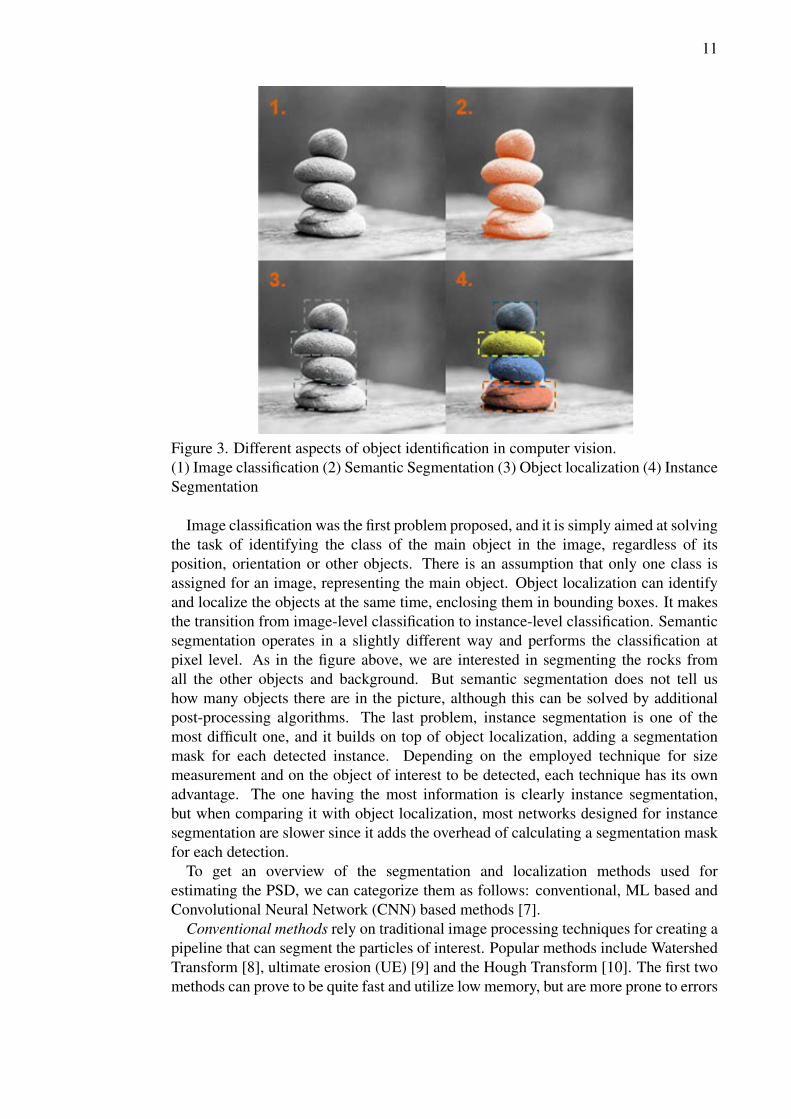
Figure 3. Different aspects of object identification in computer vision.
(1) Image classification (2) Semantic Segmentation (3) Object localization (4) Instance
Segmentation
Image classification was the first problem proposed, and it is simply aimed at solving
the task of identifying the class of the main object in the image, regardless of its
position, orientation or other objects. There is an assumption that only one class is
assigned for an image, representing the main object. Object localization can identify
and localize the objects at the same time, enclosing them in bounding boxes. It makes
the transition from image-level classification to instance-level classification. Semantic
segmentation operates in a slightly different way and performs the classification at
pixel level. As in the figure above, we are interested in segmenting the rocks from
all the other objects and background. But semantic segmentation does not tell us
how many objects there are in the picture, although this can be solved by additional
post-processing algorithms. The last problem, instance segmentation is one of the
most difficult one, and it builds on top of object localization, adding a segmentation
mask for each detected instance. Depending on the employed technique for size
measurement and on the object of interest to be detected, each technique has its own
advantage. The one having the most information is clearly instance segmentation,
but when comparing it with object localization, most networks designed for instance
segmentation are slower since it adds the overhead of calculating a segmentation mask
for each detection.
To get an overview of the segmentation and localization methods used for
estimating the PSD, we can categorize them as follows: conventional, ML based and
Convolutional Neural Network (CNN) based methods [7].
Conventional methods rely on traditional image processing techniques for creating a
pipeline that can segment the particles of interest. Popular methods include Watershed
Transform [8], ultimate erosion (UE) [9] and the Hough Transform [10]. The first two
methods can prove to be quite fast and utilize low memory, but are more prone to errors
12
and susceptible to noise in images. On the other hand, Hough Transform can be more
robust, but is slower and has a large memory footprint. The big disadvantage shared by
all these conventional methods is having to adjust parameters by the user, depending
on the imaging conditions, the particles to be observed and other major changes in the
operating environment. These type of algorithms are unfortunately not robust enough
by themselves and any change can potentially lead to erroneous results, meaning that
the system needs to be recalibrated each time. Moreover, fine-tuning the parameters
can be time-consuming and if performed frequently, it can become a major bottleneck.
ML-based methods [11, 12] are one step closer towards making the process more
autonomous, since there are very few image or environment dependent parameters that
need to be set by the user. ML-based methods rely on two key concepts, namely feature
extractors and classifiers. The classifiers are trained with the extracted features, finding
patterns in the input data. Then, based on the learned features, the classifiers will label
unseen data. Descriptors are usually used as input data to the ML classifiers, meaning
that a lot of effort is shifted towards designing efficient and robust descriptors, capable
of capturing as much information as needed. By compressing parts of images in
descriptors, the available information is reduced, affecting the accuracy of the model.
CNN-based methods are end-to-end methods that can learn not only feature
interpretation, but feature extraction as well. This means that there are virtually no
parameters that need to be set by the user, as CNN methods work directly on the raw
image. On the other hand, they are heavily dependent on vast amounts of annotated
data, so that the model can extract useful information. Getting enough data for every
application where CNNs are used can be very tricky and most of the time even
impossible. But, a good technique to overpass the lack of data is transfer learning,
where a model is trained on general purpose data with the objective of learning the
feature extraction and later training only the last layers on the specific, reduced dataset
for our application. This will be discussed in detail later on.
There are also hybrid methods, that combine the principle of laser diffraction with
imaging techniques. In [13], the authors built a particle analyzer using a CMOS
image sensor and a collimated beam configuration, together with a ML model based on
Random Forest. Similarly to laser diffraction, they have used the angular distribution
of scattered light to measure particle size.
2.4. Limitations of Traditional Image Processing Methods
Image-based analysis proves to offer enough information and data for estimating the
PSD accurately and robustly, but even after choosing this approach, there are a wide
range of algorithms that can achieve the segmentation of an image. Conventional
methods based on traditional image processing techniques were the founding blocks
of image-based analysis. But, they soon proved to be difficult to develop, maintain
and transfer the same concept or pipeline to a new setup, even though the requirements
were the same. One of their main disadvantages is the huge number of parameters
involved. Each step in a general pipeline requires several parameters to be adjusted, for
example, image smoothing, edge detection, thresholding, morphological operations,
labelling, etc. Not only does this make the development hard, but a slight change
in the working environment may affect the pipeline altogether and crash the system.

13
Moreover, none of these methods can compete with the accuracy of a human operator
[11].
A more robust approach is to use machine learning algorithms, that are able to better
predict properties of objects in the image or even classify them. These algorithms have
an increased tolerance for changes in the working environment and can better handle
unknown data. But, ML algorithms are also dependent on the extracted features and
part of the workload does not disappear, but is actually shifted towards designing robust
and efficient feature extractors and descriptors. While having far fewer parameters to
tune than traditional image processing techniques, there is still a number of parameters
that need to be set for the feature extractors and classification models and sometimes
designing the perfect features extractor can be quite time consuming.
Because of all these inconveniences, end-to-end methods are really desired in the
industry. Working conditions can change, especially in industrial environments, so
increased flexibility is needed. Also, there are a lot of mineral processes that have a
high degree of similarity and rather than designing a completely new system for each
in turn, it would make sense to transfer the core concept and adjust as few parameters
as possible. DNNs are pushing forward the state-of-the-art in computer vision and
are enabling end-to-end methods, where users only need to feed annotated data and
then the network is capable, on its own, of extracting the features, learning them and
ultimately classifying new data.

14
3. DEEP LEARNING BASED INSTANCE SEGMENTATION
The computer vision community has seen a great increase in the utilization of DL in
last years and starting from the success of AlexNet [14] in the ImageNet competition
(Large Scale Visual Recognition Challenge, ILSVRC 2012 [15]) it has since been the
hot-topic of computer vision. Not only has DL extended to other tasks in computer
vision such as object detection and localization, semantic segmentation, instance
segmentation, pose estimation, and so on, but it has been successfully applied in
other domains as well, such as audio [16], natural language processing (NLP) [17],
3D reconstruction [18] and many others. Keeping in mind the recent advancements in
terms of GPU processing capabilities, it becomes more and more clear that DL is for
now, the tool of choice for solving the problems of today and tomorrow.
Because DL is such a vast domain, the next section will be focused on a brief
overview of the core idea behind DNNs and how they have evolved in the context of
machine learning and under the big umbrella of artificial intelligence. The explanations
will start from the building blocks of DNNs, then gradually going through state-of-
the-art architectures. Popular DL models will be presented, with applicability in the
instance segmentation domain.
3.1. AI Vs. ML Vs. DL
The concept of Artificial Intelligence was born in the 1956 by the AI pioneers
who envisioned complex machines capable of expressing human intelligence. This
means sensing, interacting with the real-world and taking human-like decisions.
Conceptually, this is known as ’General AI’ and would ideally be represented as
machines that can behave and reason like humans do. For now, this theoretically and
maybe frightening concept cannot be achieved, but instead, more specialized forms of
AI have been developed for particular scenarios and tasks, like image classification,
text recognition, natural language processing, robot control, etc. These are still tasks
or actions that require human-like intelligence, hence the algorithms based on DL are
built specifically for a task, rather than building a ’general AI’ robot that can solve
everything.
Figure 4. Venn diagram describing the relationship of the three concepts: AI, ML and
DL.
Machine learning is a subset of AI practices that shifts the paradigm from hand-
programming to data learning. Rather than designing algorithms to behave in a certain

15
way, ML algorithms learn from the available data and then make educated guesses on
unseen data. This consists of parsing the data, learning different patterns that are likely
to occur by extracting features from data and then make a prediction about previously
unseen data. ML encapsulates a wide set of algorithmic approaches, like clustering,
reinforcement learning, decision-tree learning, feature-based learning, etc. Although it
is more robust and flexible than previous methods, it still involves a lot of hand-coding
and crafting of feature extractors.
Parts of the ML tool set are also Artificial Neural Networks (ANNs). They are
inspired by the way in which our brain functions, leveraging the inter-connection
between multiple neurons. In a Neural Network (NN), the neurons have weights
associated with each of them and represent how wrong or correct it is relative to
the performed task. Even though they were present from the early days of AI, the
hardware was not yet ready for supporting this concept. The most basic networks
were too computationally intensive and they were simply not feasible. With the
deployment of GPUs, specialized hardware for parallel processing, the breakthrough
of ANNs and specifically very deep ANNs (DNNs) was possible. Networks with
increased number of layers and neurons were possible to train in reasonable times and
some architectures proved to perform even better than humans in some tasks (image
classification). But there is a twist. Deep neural networks require huge amounts of
data, usually being trained on hundreds of thousands of images which requires them
to be labelled. As the task increases in complexity, e.g. from image classification
and up to instance segmentation and panoptic segmentation, the labelling process
becomes more difficult and requires more time and resources. Also, when applying
DL to a specialized, narrow domain, like mineral detection, there are few challenges
like manual annotation, lack of available data, complexity of labelling, ambiguity in
labelling and others.
3.2. Neural Networks
The building block of a neural network is the neuron. Inspired from biology, the neuron
takes as input stimuli from multiple connections and when sufficient stimuli, it fires
on the output. Likewise, in ANNs, a node (neuron) multiplies input data with a set
of weights associated with every connection, trying to amplify or dampen that input,
based on its significance relative to the performed task. This allows the network to
characterize which input is helpful when classifying. The sum of product between
weights and data is passed through an activation function that decides if or how much
of the signal should pass onward. This can be mathematically formulated as:
y = θ(b+N∑
i=1
xiwi) (1)
where y is the output of the activation function, xi are the inputs, wi are the weights of
the networks, b is the bias and ultimately, θ is the activation function. Visually, a node
representation is depicted in Fig. 5a.

16
(a) Node of a neural network (b) Neural network structure
Figure 5. Generic structure of a neural network.
A NN is formed by stacking layers of neurons and connecting the layers. A generic
architecture for a NN consists of an input layer, which consumes the input data, hidden
layers and ultimately an output layer responsible for the prediction (represented as
probability). A DNN is basically a NN that has many hidden layers, hence the name
’deep’. The motivation behind building deep neural networks is that the deeper you go
in a neural net, the more complex features nodes can learn, since they are aggregated
with previous nodes. Training is an iterative process that updates the weights and
biases such that the loss function is minimized and the data is learned.
3.2.1. Activation Functions
If we think about Eq. 1 and ignore the activation function, a neuron is just computing
the weighted sum of its input, obtaining a real number. Same as a biological neuron,
an artificial neuron needs to decide whether it fires or not (it is activated or not). The
mechanism allowing this is the activation function. There are two types of activation
functions: linear and non-linear functions. The non-linear functions are mostly used
due to their ability to generalize or adapt to the variety in data. Below, some of the
most used activation functions are presented, alongside their graphs.
The sigmoid function is defined by:
f(x) =1
1 + e−x
It outputs a value between 0 and 1, it is non-linear, continuously, differentiable and
monotonic, all being desirable properties of an activation function. A big drawback is
the insignificant change in gradient for inputs that are far from the origin. This gives
rise to the problem of vanishing gradient, where the network is not capable of properly
learning anymore or the training becomes increasingly slower for saturated neurons.
A similar function, the hyperbolic tangent, is also a non-linear function, but unlike
the sigmoid, it is zero-centered, resulting in a better mapping of negative/positive
values, making them strongly negative/positive. Unfortunately, it also shares the
problem of vanishing gradient. Its mathematical definition is:

17
f(x) =ex − e−x
ex + e−x
Rectified Linear Units or ReLU, may sound complicated, but it can be easily
formulated as just:
f(x) = max(0, x)
It is non-linear, and has the same advantages as the sigmoid, but proves to have better
performance. Also, it does not suffer from saturation and it is much easier and faster to
compute the gradient. On the other hand, it is suffering from the well-known problem
of "dying ReLU". In the case of having an input x < 0, the gradient will be 0, which
means the weights will not be adjusted. Hence, those neurons will stop responding to
variations in input. Leaky ReLU is a variant of ReLU where a small, non-zero gradient
α is allowed when the input is below zero.
(a) Sigmoid (b) Tanh
(c) ReLU (d) Leaky ReLU
Figure 6. Graphs of activation functions.
3.3. Architecture of DNN
As it was mentioned in Section 3.1, general AI is rather a sci-fi dream than reality and
the same is true for DL. There is no ’good-for-all’ architecture and because of that, a
range of different techniques have been developed for specific tasks that can boost the
efficiency of a DNN. In this section, the most representative techniques are presented.
18
3.3.1. Convolutional Neural Networks
Convolutional neural networks (CNN) or ConvNets, have gained massive attention in
computer vision and serve as basis for state-of-the-art architectures like AlexNet [14],
VGGNet [19] or GoogleNet [20]. The components of a CNN are usually: convolution
layer, pooling layer and fully connected layer. One of their main advantages is the
capability of capturing both the spatial and temporal dependencies in an image by
applying various filters. Since the core concept of ConvNets relies on reducing the
number of parameters, therefore retaining only the most important features, CNNs can
better fit the data than traditional NNs.
Convolutional layer
The convolutional layer is the most important part of a CNN. It relies on the
convolution operation [21] to convolve the input image with different filters and obtain
activation maps, which are in turn convolved again and again. Similarly, as in a
neural network, a neighborhood or spatial region of the image, regarded as the input
is convolved (multiplied) with the filter coefficients (weights). Then, an activation
function is applied and the results are getting propagated through the network, similarly
to a NN. The main objective of the convolution operation is to extract the high-level
features such as edges or blobs. A convolution layer consists of a stack of filters,
each with weights wi, that will be the weights of the neural network that have to be
learned. The spatial region on which we apply the convolution is called the receptive
field. Different than in a Multi Layer Perceptron (MLP), where the output of a neuron
depends on all the values from the previous layer, in a convolutional layer, the output
depends on the filter i, specifically its weights, and the receptive field on which it
is applied. The convolution operation usually decreases the dimensionality of the
convolved feature, although padding can be used to either increase the dimensionality
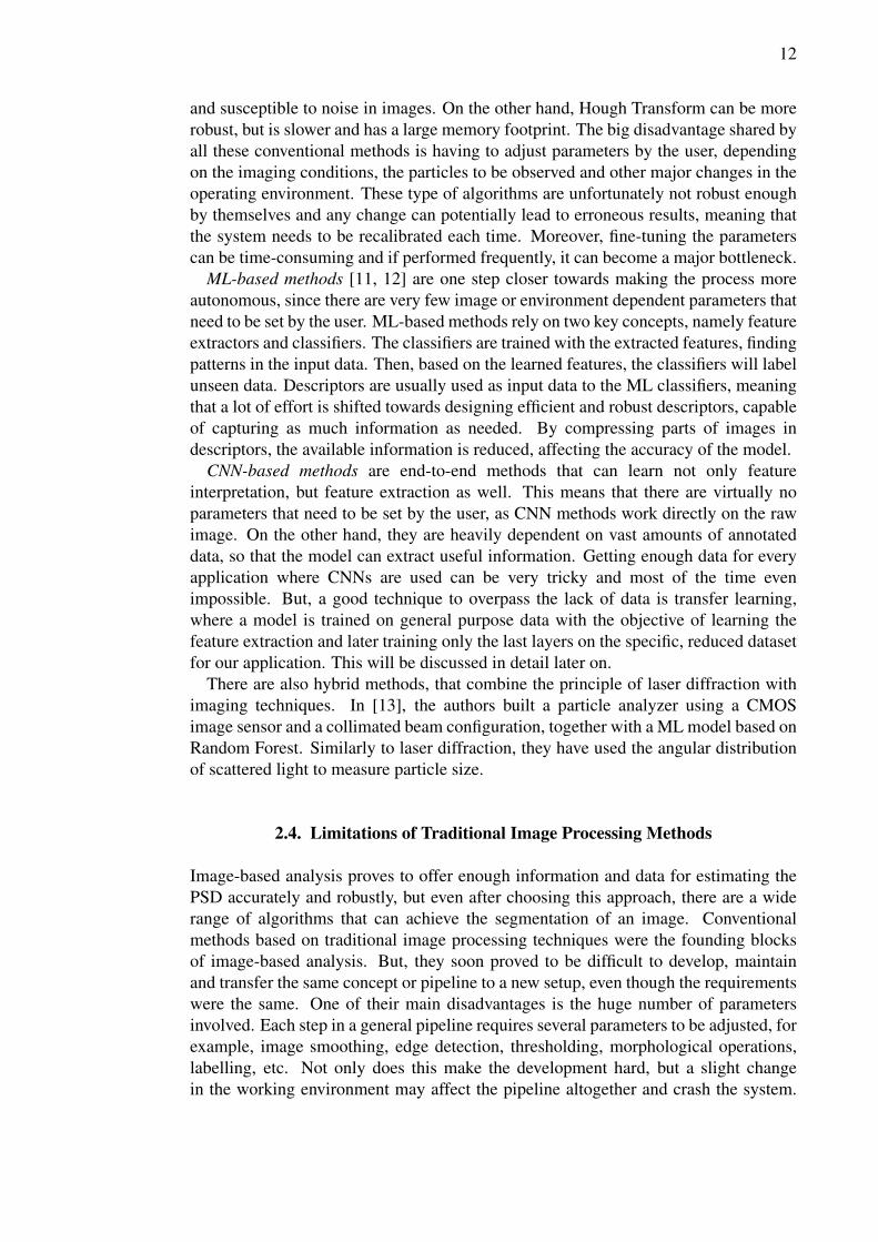
or keep it the same. In Fig. 7, a convolution with two 5x5x3 filters is applied.
Figure 7. Convolution of a 32x32x3 image with two 5x5x3 filters with stride 1 and no
zero padding, that produces two activation maps.
The key parameters for a convolutional layer are the stride and padding. The stride
is used for selecting the overlap between receptive fields and the padding, which is
usually performed with zero values, is used to increase the size of the input, so pixels

19
situated near the border are considered as well. Using the following equation, one can
determine the output of a convolutional layer:
(w + 2 · p− k)/s+ 1,
where w is the size of the input, k is the size of the kernel, p is the size of the padding
and s is the stride.
Pooling layer
The pooling layer is responsible for down-sampling the input, reducing the spatial
dimensionality. This is desirable for concentrating the information and retaining
only what is considered to be most important, such that the network can learn more
efficiently. Usually, it is placed after a convolutional layer. Also, by down-sampling,
we obtain multi-resolution maps that can yield different important features. The
most used operator is the max-pool one, retaining only the maximum value in the
receptive field. Min and (global) average pooling are also applied, but are less frequent
[22]. There are also studies in favour of dropping the pooling layer, especially when
training Generative Adversarial Networks (GANs) or variational AEs, in favour of
using convolution with bigger strides [23, 24].
Figure 8. Pooling operation down-samples the input. Here, the input is downsampled
using a max-pool filter with stride 2.
Fully connected layer
The fully connected layer is usually used in the last stage of a CNN and is often
responsible for outputting class membership probabilities. It works in the same way
as a neuron in a MLP, taking into account all the input nodes from the previous layer.
The last vector obtained by convolution and pooling is usually flattened and then fed
to the fully connected layer, where a softmax function is applied.
3.3.2. Residual Block
A rule of thumb in deep learning was that the deeper the network is, the better it
performs in terms of accuracy. This technique was preferred by researchers because of

20
its simplicity, but it proved to work only until a certain depth level. If the network
is too deep, then problems like vanishing/exploding gradients or degrading appear
[25, 26]. Vanishing gradient can happen if the weight initialization or data pre-
processing steps are not done properly and also when applying the chain-rule over
many stacked layers, then the gradient will get to zero eventually, resulting in the
network not learning properly. Another problem that happens in Recurrent Neural
Networks (RNNs), is the exploding gradient, where if we unroll the RNN for a
number of steps and observe what the backward pass is doing, we can see that the
gradient signal is getting multiplied many times with the same matrix, which can
lead to the gradient ’exploding’. Certain techniques have been developed to combat
these problems and enable networks to converge using stochastic gradient descent
(SGD) [27] by using normalized initialization and intermediate normalization layers
[28] (batch normalization). Degradation, in terms of training accuracy, was observed
when more layers were added, but the accuracy saturated or even started to decrease
dramatically [29].
Figure 9. Residual block. Copyright c© 2016, Reprinted with permission from IEEE.
This problem was addressed by K. He et al. [30], which introduced a deep
residual learning framework and were the winners of ILSVRC-2015 [15] classification
task. Instead of simply stacking multiple layers on top of each other in the hope
of learning an underlying mapping, they fit a residual mapping. This is done by
adding a skip connection, also known as identity shortcut connection, as in Fig. 9.
In their case, the skip connection just performs an identity mapping adding, where
their outputs are added to the outputs of the convolutional layers. This way, instead
of learning the desired underlying mapping H(x), the eq. F(x) + x is learned, where
F(x) := H(x) − x is the residual mapping and authors claim that it is easier to learn
the residual mapping than the original one. Hence, this framework enables the network
to be trained end-to-end using backpropagation with SGD and no extra parameters or
computational complexity is added by the shortcut connections. Moreover, the residual
learning framework is generic and can be applied to other architectures as well.
3.3.3. Feature Pyramid Network
One of the biggest problems in the object detection task is being able to recognize
objects at different scales. Especially for small objects, it can be hard for detectors to
recognize them. A popular technique consists in building a pyramid of different image
scales [31]. Then, processing each level in the image pyramid, objects at different
scales can be detected. In practice, this approach has some drawbacks. Regarding
performance, building an image pyramid takes significant time and memory and this

21
creates a problem for real-time applications. Also, as we go higher in the pyramid,
the resolution decreases and the semantic value increases because of the high-level
structures detected, but we cannot use bottom layers since the semantic value is low,
although the resolution is higher.
A robust solution for this problem is the Feature Pyramid Network (FPN) [32].
FPN is a feature extractor that satisfies the requirements of speed and memory. As
it can be seen in Fig. 10, it consists of a bottom-up and a top-down pathway, with
lateral connections. The bottom-up pathway is pretty intuitive, enriching semantically
each higher level while decreasing the resolution. The top-down pathway aims at
reconstructing higher resolution layers from semantic rich layers. In terms of accuracy,
the reconstructed layers are not so precise because of the upsample/downsample
operations, so lateral connections are used to better predict the locations of objects.
Similar as in ResNet, the lateral connections act as skip connections, making training
easier. As a result, the architecture is able to build a feature pyramid with rich semantic
features at all levels from a single input image scale. Another great advantage of FPN
is being a generic solution that can be applied to many problems and architectures,
like RPN (Region Proposal Network), R-CNNs (Region based Convolutional Neural
Networks) or extracting masks for image segmentation.
Figure 10. FPN Architecture. Copyright c© 2017, Reprinted with permission from
IEEE.
3.4. Related Work
This section will give an overview of the evolution of Mask R-CNN, starting from
the simple R-CNN and analyzing all the intermediate architectures which eventually
led to the creation of the aforementioned. Yolact architecture will also be discussed
as an alternative to Mask R-CNN and key differences will be highlighted, especially
regarding those that affect the processing time.
3.4.1. From R-CNN to Faster R-CNN
Object detection in computer vision is still one of the greatest challenge, since it is
also the foundation of other tasks, like instance segmentation or size distribution of
objects. Because we cannot assume the number of objects to be detected in an image,
it is impossible to use a ConvNet with a fully connected layer and have as input only

22
one image. Multiple patches from an image could be used, but the question is how to
choose them smartly in terms of aspect ratio and spatial location, since a brute-force
method would be too computational intensive.
In [33], R. Girshick et al. proposed R-CNN, which stands for Regional-based
Convolutional Neural Networks. R-CNN uses selective search [34] to extract only
2000 regions from an image which will represent region proposals. Their system
consists of three modules. The first one is the region proposal generator, which
fabricates 2000 candidate regions. Then, each region is fed to a CNN, which acts
as a feature extractor and outputs a fixed-length vector as output. The last module is
a set of class-specific linear SVMs, that classifies each region and also regresses four
values, representing an offset of the bounding box, such that the location precision of
the bounding box is increased.
Figure 11. R-CNN. Copyright c© 2016, Reprinted with permission from IEEE.
The same author, in [35] managed to solve the problem of processing many region
proposals by feeding the input image to the CNN, which generates a convolutional
feature map. Then, region of proposals are identified from the convolutional feature
map and a RoI pooling layer reshapes them into a fixed size by warping, so that they
can be connected to a fully connected layer. Now, having a RoI vector, a softmax layer
is introduced to predict the class and in parallel, a bounding box regressor finds the
optimal offset. The new architecture is depicted in Fig. 12. These modifications allow
the training to be single-stage, using a multi-task loss and the training can update all
network layers.
Figure 12. Fast R-CNN. Copyright c© 2015, Reprinted with permission from IEEE.
Another notable attempt at speeding up R-CNN was the use of SPP nets [36]. Like
Fast R-CNN, the SPP net computes a convolutional feature map from one image,
23
computes a feature vector for each object proposal and then classifies it using SVMs.
Again, we have a multi-stage pipeline that takes significantly more time to train.
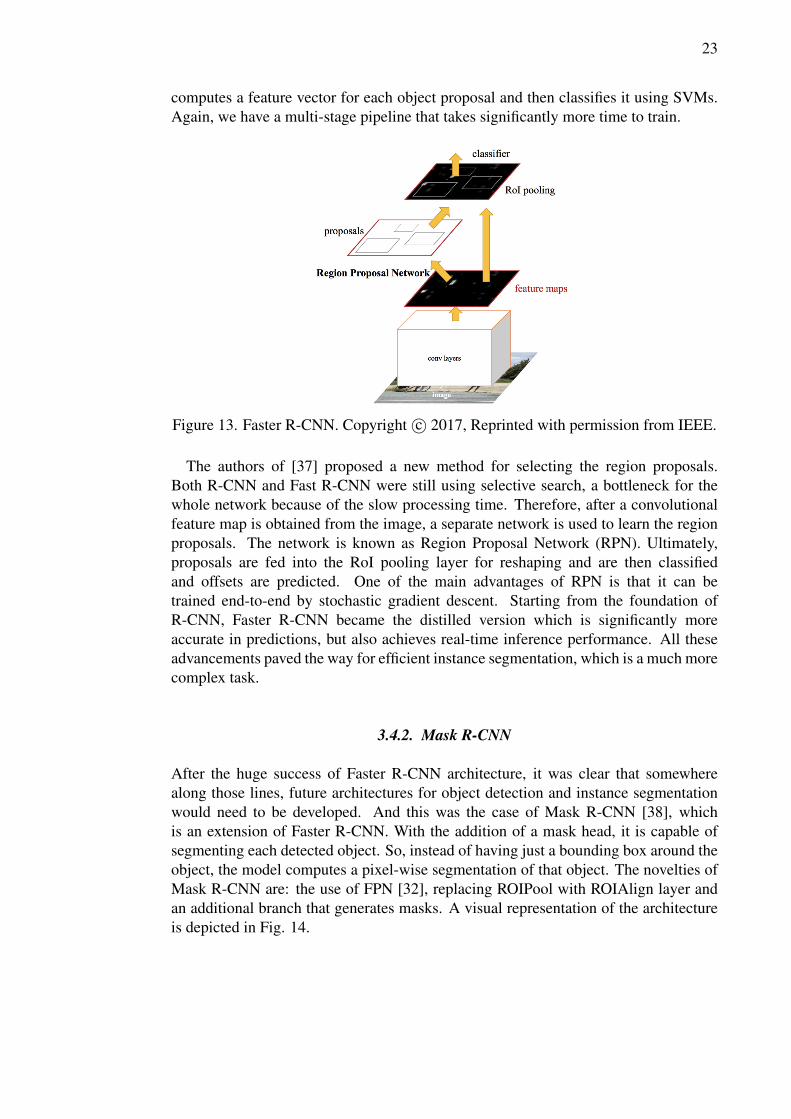
Figure 13. Faster R-CNN. Copyright c© 2017, Reprinted with permission from IEEE.
The authors of [37] proposed a new method for selecting the region proposals.
Both R-CNN and Fast R-CNN were still using selective search, a bottleneck for the
whole network because of the slow processing time. Therefore, after a convolutional
feature map is obtained from the image, a separate network is used to learn the region
proposals. The network is known as Region Proposal Network (RPN). Ultimately,
proposals are fed into the RoI pooling layer for reshaping and are then classified
and offsets are predicted. One of the main advantages of RPN is that it can be
trained end-to-end by stochastic gradient descent. Starting from the foundation of
R-CNN, Faster R-CNN became the distilled version which is significantly more
accurate in predictions, but also achieves real-time inference performance. All these
advancements paved the way for efficient instance segmentation, which is a much more
complex task.
3.4.2. Mask R-CNN
After the huge success of Faster R-CNN architecture, it was clear that somewhere
along those lines, future architectures for object detection and instance segmentation
would need to be developed. And this was the case of Mask R-CNN [38], which
is an extension of Faster R-CNN. With the addition of a mask head, it is capable of
segmenting each detected object. So, instead of having just a bounding box around the
object, the model computes a pixel-wise segmentation of that object. The novelties of
Mask R-CNN are: the use of FPN [32], replacing ROIPool with ROIAlign layer and
an additional branch that generates masks. A visual representation of the architecture
is depicted in Fig. 14.

24
Figure 14. Mask R-CNN framework [38]. Copyright c© 2017, Reprinted with
permission from IEEE.
Mask R-CNN shares the same two-stage type procedure as Faster R-CNN. In the
first one, RPN is responsible for generating region proposal, then in the second one,
the class and bounding box offsets are predicted in parallel, with the addition of a mask
predictor that works in parallel. Because of that, the multi-task loss is defined as:
L = Lcls + Lbox + Lmask
The mask branch is unique in the sense that it generates masks for every class, hence
there is no competition among classes and the classification is left to the class predictor.
By doing this, mask and class predictions are decoupled, unlike usual FCNs [39],
where a per-pixel softmax and multinomial cross entropy loss is used. Different than
Fast R-CNN, pixel-to-pixel alignment is of high importance, which led the authors to
propose ROIAlign, a layer responsible for aligning the extracted features with the input
and getting rid of the aggressive quantization introduced by ROIPool.
A closer look at the architecture reveals that RPN is not applied on the original input
image, but rather a backbone is used for extracting feature maps and subsequently,
RPN scans over the backbone feature map. A backbone is a convolutional neural
network that acts as a feature extractor, producing feature maps, which are passed
further down the network. In terms of backbone architectures, the authors experiment
with ResNet [30] and ResNeXt [40]. They also use a FPN [32], such that RoI features
are extracted at different levels of the feature pyramid, resulting in substantial accuracy
and speed improvement.
In [41], authors discover an inconsistency in assigning the score of an instance
mask by using the box-level classification confidence. The confidence score takes into
consideration only the difference between the semantic categories, and it is oblivious
to the quality of the instance mask. For example, we might get a good bounding-
box localization and a high classification score, but the mask quality can vary. This
can further impact the evaluation and the training procedure. In the COCO [42]
challenge, the evaluation is done by taking the average precision (AP) metric that
uses Intersection-over-Union (IoU) score between the prediction and the ground-truth
mask, but that is calculated for a fixed confidence threshold score. So, inspired by
this, the authors propose a network capable of directly learning the mask IoU score
and combining it with the confidence score as well, resulting in an alignment between
the mask quality and its score. By addressing the problem of instance scoring, their
solution improves the Mask R-CNN framework.

25
3.4.3. Yolact
Initial experiments using Mask R-CNN for the task of particle detection proved to be
promising, but there was another requirement that had to be taken into consideration
for the purpose of the overall system and that is the speed of processing. To
efficiently monitor the PSD in the grinding process, real-time processing is mandatory,
specifically in our case, we would need to process at least 10 frames per second (FPS).
Bearing in mind this requirement, using Mask R-CNN is not feasible anymore since
it can process 5 FPS on a beefy GPU. For this, the attention is shifted towards an
architecture that is able to offer real-time processing without sacrificing too much
accuracy. And Yolact [43] is the perfect candidate.
Fig. 15 depicts a comparison in terms of FPS vs. mAP on the COCO dataset. It
can be easily seen that Mask R-CNN has a very good mAP score, but it lacks in speed.
On the other hand, Yolact offers the best trade-off between accuracy and speed of
processing. Another aspect that needs to be taken into consideration is the GPU on
which the performance results are computed. All these comparisons have been done
on beefy GPUs and considering our use case, it may be more feasible to have more
compact processing units, like embedded GPUs, which do not have the same high
processing power and memory capacity, so it is expected for the FPS rate to decrease
when the model is deployed on such GPUs.
Figure 15. Comparison of various architectures in terms of speed and mAP [43].
Copyright c© 2019, Reprinted with permission from IEEE.
Previously, it was shown that Mask R-CNN is a two-stage detector, that relies on
feature localization to generate masks. Only after the features have been re-pooled
in the bounding-box region, they can be fed to the mask predictor, resulting in a
sequential pipeline that represents a bottleneck in speed. To overcome this, D. Bolya
et al. proposed Yolact [43], a single stage instance segmentation model capable of
achieving real-time performance.
In order to achieve real-time performance, the authors break up the task of instance
segmentation in two, parallel stages that are finally combined with minimum overhead.
The overall architecture is presented in Fig. 16. The common parts of the network are

26
the backbone used for feature extraction and the FPN for producing more robust masks
and high resolution prototypes. Then, in parallel, prototypes and mask coefficients are
generated.
Figure 16. Yolact Architecture [43]. Copyright c© 2019, Reprinted with permission
from IEEE.
Protonet is the network responsible for the generation of k prototypes. It is
implemented as a FCN which has k channels in the last layer and uses as input
a backbone feature layer, enhanced by the FPN. Although this looks similar to a
semantic segmentation task, it differs by having no loss over the prototypes, instead the
optimization is done from the final mask loss, that is calculated after assembly. Mask
coefficients are generated in parallel to Protonet. Being an anchor-based detector, it
has two branches in the prediction head, namely classification and bounding-box offset
regression. To compute mask coefficients, another branch is added, in parallel to the
other two. In the final step, the masks are assembled by combining the prototype
branch and the mask coefficient branch. The operations are implemented as a matrix
multiplication and sigmoid:
M = σ(PCT )
where P is a h× w × k prototype masks and C is a n× k matrix of mask coefficients
corresponding to n instances that passed through Non Maximum Suppression (NMS).
In addition to the new architecture, they also propose an improved version of NMS,
called FastNMS, where the decision of keeping or not an instance is done in parallel
for all instances, therefore improving the speed performance even more. Although
this version suffers from removing a little bit too many boxes, the accuracy drop is
negligible in comparison to the huge increase in speed performance.
3.5. Particle Detection Using ConvNets
Object detection, instance segmentation and semantic segmentation techniques have
been used in a variety of real-world applications, ranging from autonomous driving,
aerial navigation to more industrial oriented applications, such as smart manufacturing
or specialized tasks in factories. Therefore, these techniques have also been used for

27
estimating the PSD in different industrial applications and have added new challenges
for these algorithms, pushing the level of innovation and demanding more research. It
comes as no surprise that methods based on DL are proving to be more efficient than
traditional methods even for this type of estimation, but they are relatively new and
ongoing research is still needed.
In [44], authors use DL for estimating the distributions of grain size and porosity
from micro-CT images. As training data, they generate synthetic 3D images of spheres,
simulating how a micro-CT image would look like. They’ve chosen a 3D CNN [45],
which was initially used for human action recognition from video images. The 3D
CNN takes as input the 3D images and outputs directly two values, the grain size
and the porosity label, hence in this case, a regression rather than segmentation is
performed. Training was done on the synthetic data and then the model was tested on
real-world data, showing promising results.
In the case of 2D images, we can also encounter the problem of partially sintered
and agglomerated particles, since the 3D particles are projected on the image plane. [7]
aims at addressing this problem by using Mask R-CNN architecture to first segment
instances of particles and to compute the PSD. The same strategy is applied as in the
latter article, training and validating on synthetic images and then testing on real-world
scanning electron microscopy images (SEM) or transmission electron microscopy
images (TEM). After inference on the test images, the PSD is calculated using the
Feret diameter as the equivalent diameter of a particle. Although the method produces
satisfying results in terms of accuracy, the time and memory requirements are not
taken into consideration and may pose a problem if this solution would be integrated
in a real-time application.
Another domain that picked the interest of deep learning and particle detection
is Cryo-electron microscopy (cryo-EM). Here, detection is difficult mainly because
of extremely low signal-to-noise ratio (SNR). The approach used in [46] is quite
unique and uses two DNNs, one classification network and one segmentation network.
First, the classification network is trained and then using its parameters as initial
values for the segmentation network, the training process is accelerated. The
segmentation network is responsible for getting probability (density) maps that are
fed to the selection algorithm (Grid-based Local-maximum selection) and produces
initial results. Ultimately, preliminary results are fed to the classification network and
final results are obtained. Similar to [47], they use ’Atrous convolution’ feature in
the segmentation network. In terms of training data, because of the low SNR which
causes very difficult manual annotation, they generate images from real-world datasets
and also use simulated datasets.
Xiao Y. proposed in [48] a solution for particle picking based on the Fast R-CNN
framework [35]. To develop a fast method, they have tried to solve one of Fast R-
CNN’s bottleneck, which was the region proposal. Instead of using selective search,
they have proposed a sliding window approach. Their solution reduces the test time
from 1.5 minutes obtained from [49] to 2 seconds. They have also tried to use Faster R-
CNN, which replaced selective search with RPN, but argued that for cryo EM images,
the RPN performs terrible and because of their special case where possible particles are
of fixed size, the sliding window is much faster and better. Also, the papers discussed
so far dealt with particle picking when there is only one particle of interest in the image,
but in this case, their images contained ice particles, which makes classification harder,

28
specifically the rate of false positives increases. To deal with that, they have annotated
ice particles as well and formulated the problem as a three-class classification, so that
the neural network would learn the subtle difference between ice and protein particles.
As a result, the rate of false positives decreased significantly.

29
4. DETAILED DESIGN AND IMPLEMENTATION
The focus of this thesis is building a system capable of estimating the PSD of mineral
rocks from images taken in a flow-through system. From a commercial point of view,
an emphasis is put on apatite particles, since they are the most valuable, but as a
challenge and to ensure generality, we take into consideration phlogopite particles as
well. For estimating the size distribution, we need to segment instances of particles
in each image. Although this can be achieved with conventional image processing
techniques, deep learning techniques prove to be much more robust, accurate and
faster, representing the state-of-the-art in the instance segmentation task. Moreover,
although semantic segmentation networks, like DeepLab [47], can also segment the
image, the dataset on which we are working includes a lot of particles that overlap
and would thus require post-processing steps that would slow the pipeline. Hence,
we choose two instance segmentation networks, Mask R-CNN [38] and Yolact [43],
both having their own specific advantages. Mask R-CNN represents the state-of-
the-art architecture in instance segmentation, but Yolact is able to achieve real-time
performance with sacrificing just a fraction of accuracy. An overview of the pipeline
applied in this thesis is depicted in Figure 17. Regarding implementation, Matterport’s
implementation [50] of Mask R-CNN has been used and for Yolact [43], authors have
released their open-sourced repository.
Figure 17. Pipeline overview.
4.1. Imaging Setup
This section will present the setup used for acquiring the data. Outotec’s PSI 500
was the device of choice, being capable of computing the size distribution using
laser diffraction, hence having a reference measurement. A flow through cuvette was
connected with a tube to PSI 500 outlet, such that the minerals are imaged in a flow-
through system. There were two setups of lightning, front lightning which emphasized
the color of particles and back lightning, which resulted in grayscale images. For
our case, we have decided to use front lightning. The camera used for capturing
images from the flow-through system had a magnification factor of 3.5 micrometers

30
per pixel. The magnification factor was important for aligning the size distribution
obtained from images with the real-world scale and also to compare it with the size
distribution obtained by PSI 500. The dataset consisted of colour images, having a
resolution of 2448x2048. Fig. 18 shows an example of captured images.
(a) Raw image data. (b) Annotated image.
Figure 18. Images captured by PSI 500 and annotated with VIA tool.
4.2. Task Description
For this use case, there are 2 particles of interest, namely apatite and phlogopite. By
looking at Fig. 18, one can already start discriminating between them. Apatite particles
are more transparent and clear while the phlogopite particles are mostly opaque and
have a brownish tint. The central task of this project is getting the size distribution
of apatite particles across a sample of images. The stakeholders are mainly interested
in apatite detection because phlogopite is much less valuable, therefore it is not so
relevant for the grinding process. On the other hand, training an algorithm to detect
phlogopite as well, may result in increased accuracy and may serve well for other use
cases, where multiple different particles may need to be detected. Hence, the task is
now formulated as a two-class instance segmentation problem.
The dataset consists of hard and tricky cases as well, where particles can be
occluded, partially captured in the image and even particles that are mixed or hard
to classify because of similarity. When particles are occluded or partially captured in
the image, it represents a problem for the PSD because we do not know its actual size,
hence we may alter the accuracy of the PSD. In our case, it was decided that particles
laying on the border of the image can be discarded, provided that we have enough
detected particles so that the result is statistically meaningful. Mixed particles are also
interesting, because one can be interested in detecting the ratio of apatite/phlogopite
from the particle or simply label it as mixed. There are also difficult particles to classify
even for a human operator. Some can be semi-transparent and have a faint tint of
brown, so it may be really difficult to assign one class. Another major challenge
for this dataset is represented by making the distinction between a particle that is
in-focus and out-of-focus. Because every measurement that it is performed needs
to be converted to a real-world scale, for particles that are not in-focus we cannot
approximate correctly their true size. The magnification factor is known only for the
31
region where particles are in-focus, everything else cannot be estimated by a simple
linear adjustment. Therefore, only particles that are in-focus need to be detected, so we
can get a reliable PSD. In Fig. 18, particles of interest are highlighted and annotated
manually.
An important note is the lack of 100% correct ground-truth, since the provided
dataset does not include annotations as well, hence particles need to be manually
annotated, with limited knowledge in the domain of mineral processing. The only
reference measurement available is the PSD provided by PSI 500, which unfortunately
cannot discriminate between apatite and phlogopite and computes the PSD considering
both particles and using the technique of laser diffraction.
4.3. Dataset Description
The datasets of images were provided by Outotec. There are 5 datasets, each having a
different ratio of apatite and phlogopite particles, measured by another system. For
each of the dataset, a reference measurement was provided by using the PSI 500
particle analyzer, namely a graph consisting of particle size (µm) and their frequency,
which can be seen in Figure 24. Because the data had to be manually labelled, only one
of the dataset was labelled and the others were used only for running the inference on
the trained model and getting the particle distribution for comparison with the reference
measurement. The only difference between the datasets was the distribution of apatite
vs. phlogopite particles. As a result of the similar structure between datasets, it allows
for easy transfer learning. For training a model, the dataset would need to be split in
a training, validation and test set. A proportion of 60-20-20 was chosen, having 72
training images, 30 validation images and 33 test images.
4.3.1. Annotation Process
When dealing with DL models, one of the most common problems is data. For a model
to be able to learn and to generalize well, a relatively big dataset is needed. There are
a number of big datasets on the internet, like COCO [42], ImageNET [15], Cityscapes
[51] and so on, but they cannot contain all the images from all domains, but they are
rather intended as natural images, containing everyday scenes/objects. Hence, in the
case of real-world data and specialized domains, researchers have to manually label
their specific dataset, which in many cases is a laborious work. Also, depending on the
task, from object detection to instance segmentation, the annotation can be more and
more challenging. In the case of image classification, it can be fairly quick to label
images, but going to instance segmentation, where one has to draw polygons carefully,
it can take significant time, especially if we have lots of instances per image, and we
need to label hundreds of images. For labelling the data, the VIA labelling tool [52]
has been used, where one can draw polygons around the object of interest. Generating
bounding boxes afterwards is really easy. The software exports the annotations in
JSON format and can be directly used in Matterport’s implementation. When training
the Yolact model, the implementation expects COCO-style annotations, therefore a
script for converting the VIA annotations to COCO annotations was implemented.

32
When annotating the images, although the annotation task is fairly easy, few
challenges were encountered. First of all, there are no clear guidelines to distinguish
between the apatite or phlogopite particles. As a rule of thumb, the apatite particles are
clear and transparent, while the phlogopite ones are less transparent, sometimes opaque
and have a brownish color. Unfortunately, there are also particles that are mixed and
contain both apatite and phlogopite, or the brownish color cannot be clearly seen. All
of these are increasing the complexity of the annotation process.
Another challenge involved the annotation of particles that are not in-focus. The
reason for not wanting particles out of focus is that after the segmentation, the particles
need to be measured and then multiplied with the magnification factor of the camera.
Particles that are not in focus do not have the same magnification, hence including
out of focus particles will alter the accuracy of the PSD. Because of the small focus
area, it was very hard in some cases to distinguish between what is in focus and what
is out of focus. In some cases, large particles were partly in focus and partly out of
focus because of their size. Another difficult case is when the particles are overlapping.
Not only do they influence the color of one another, but sometimes it can be hard to
correctly guess and label its true contour.
4.3.2. Dataset Analysis
Matterport’s implementation of Mask R-CNN offers scripts for analysing the dataset,
which helps in carefully setting some of the network’s configuration parameters. The
first analysis is carried on the mean value of all the pixels in the dataset, for each color
channel. This value is useful for mean subtraction, as part of the network preprocessing
steps. This also had to be done for Yolact as well. If we are dealing with images of
multiple dimensions, we also need to analyse their dimension and choose the optimal
size, as input images are resized to one size, so the model can be trained with multiple
images per batch. Other statistics, such as number of particles per image or per dataset
can be obtained, which can be useful for the evaluation of the network. A function
for computing the bounding box distribution was also added, as this allows for better
choosing the anchor scales. The anchors can be overlaid on the input images, so we
can hint how they are covering the feature maps. Unfortunately, Numpy uses bytes
for Boolean values, resulting in large masks for high resolution images, making the
training really slow. For this, mini masks are used (resize masks to a smaller scale e.g.
56 × 56). They can also be inspected to see which mask size achieves the optimal
trade-off between accuracy and low memory.
The size of particles was also analyzed by plotting the histogram of equivalent
diameters. Figure 19 reveals that most of the particles have the equivalent diameter
less than 290 pixels, which translates to roughly 1 mm in metric scale. The maximum
size that can be detected by PSI 500 is 1 mm, but by looking at the histogram, the
imaging system allows for identifying even larger particles.

33
Figure 19. Particle size histogram for the training dataset.
4.3.3. Transfer Learning
As mentioned above, the size and quality of data play a major role in building a good
DL model. State-of-the-art DNNs require thousands of labelled images, which in some
cases, as in this work, is just impossible to get.
Transfer learning paradigm [53, 54] hopes to offer a solution to this problem
by transferring the common features that are shared by multiple data points. This
technique consists of training a model on a big dataset, like ImageNet or COCO, and
use the weights as initial weights for training the model on a much smaller, specific
dataset. The reasoning behind why this works is that many images share the same
low-level spatial characteristics, and it is much easier for the model to learn these
features from big data. Not only it solves the problem of having a small training
dataset, but transfer learning is also a technique used for preventing overfitting. In this
work, pre-trained weights of models trained on COCO and ImageNet have been used,
but the difference in accuracy between them is negligible considering the use case of
this thesis.
Depending on the implementation and models, in some cases a restrictive rule is to
have the same image size as the images on which the pre-trained model was trained. In
the case of Matterport’s implementation, that was not an issue, but in the case of Yolact,
only 550x550 or 700x700 images can be used. Therefore, that means scaling down the
images from 2448x2048 to 550x550, which greatly affects the quality of the images
and annotations. Especially smaller particles became so small that it was impossible to
visually localize them, while the blurriness was accentuated a lot. Moreover, rescaling
the dataset makes the comparison between models a bit more difficult and inconsistent.

34
4.3.4. Data Augmentation
Transfer learning solves the problem of having huge data for training, but it works
until a certain moment. While it can transfer low-level spatial features, we still need to
deal with the high-level ones. And even for this task, the available dataset was really
small, namely only 73 images for training. Data augmentation is the technique used to
artificially generate new, similar data from existing one. The aim of data augmentation
is to increase the size of a dataset. There are two major categories of image data
augmentation according to [55], specifically basic manipulations and deep learning
approaches. In this work, the focus will be on the first one, consisting of basic image
processing techniques that alter the images in a slight way, so that the dataset size is
increased with plausible fabricated images. This process is applied only to the training
dataset as opposed to data preparation, where the same operations need to be applied to
the validation and testing dataset as well. The choice of image processing operations
needs to be taken carefully, by analyzing the context of the data. For example, it does
not make any sense to rotate a picture with a car upside-down as the model will most
surely not see anything like that.
For the training dataset, in the case of Mask R-CNN, the considered augmentations
were flipping of the image left/right, flipping up/down, rotating it, blurring, sharpening
and edge enhancement. With each new augmentation operation, the dataset doubles its
size. For the current use case, a lot of flipping and rotations can be done, since spatially,
the particles can be anywhere in the image and placed in any direction. But when
dealing with colors, it was essential to capture the brownish color of the phlogopite
as a distinctive landmark, consequently no operations altering the color channels has
been performed. If using augmentations that change the spatial location of the objects,
annotations also have to be modified accordingly. Yolact data augmentation consists
of photometric distortion, random sample crops, mirroring, flipping and rotations.
4.4. Training and Optimization
When training a DNN, the two most important metrics are training and validation loss.
They represent all the losses summed up and offer a general overview of the network
performance and how well it is learning. The losses have to be evaluated together, so
that we can choose the best model. By analyzing the training loss, we can see if the
model has started to learn or not, by how the loss converges or spikes. But a converging
training loss does not indicate the performance of the model and from a certain
point, the model actually overfits the training data, resulting in poor generalization.
The validation loss can indicate the overfitting, as it stops improving after a certain
amount of epochs and afterwards it keeps degrading. Validation loss is also used for
early stopping [56], namely stop training after there is no more improvement in the
validation loss for a specified interval.
In Fig. 20, the training and validation loss from the Mask R-CNN model are shown.
The Matterport’s implementation saves a new model whenever a better validation
loss has been recorded, so at the end of the training we are sure to get the best
model. Unfortunately, Yolact’s implementation does not provide such a feature, but
by analyzing the losses, we can select the best model.

35
(a) Training Loss (b) Validation Loss
Figure 20. Training and validation loss of Mask R-CNN model.
In Mask R-CNN, we are training the model with the full-resolution images, so that
we can accurately segment small particles as well. Because of this, we can work with
a batch size of only one image. On the other hand, on Yolact we have to work with
much lower resolution images (550 × 550) and the architecture is more lightweight,
meaning that we can have a batch size of even 8 images, which is highly recommended
by the authors. A bigger batch size usually allows for a better convergence to the local
minimum when applying gradient descent.
Other parameters, such as weight decay, learning rate, learning momentum, etc.
were left the same as in the original implementation. Adjusting different parameters
and obtaining different models can easily become hard to track and then especially
difficult to compare them. Also, visualizing independently the losses (class loss,
bounding-box loss, mask loss) can yield some insights into what may go wrong with
the training. A great tool for solving all these issues is W&B (Weights and Biases) [57].
With few lines of code, it is able to log all the desired metrics and stores them in the
cloud, offering a nice centralized visualization. This way, we can compare the losses
between different models and choose which one was the best one and what parameters
were used. It can also keep track of all the losses, so they can be inspected separately.
4.4.1. Blurry Class
When doing the evaluation of the first model, we observed an interesting fact: the rate
of false positives was significantly high, and they usually occurred when the model
was detecting out-of-focus particles. Strictly considering detection, this proves how
remarkable the network is and how capable it is of detecting a good variety of particles.
On the other hand, considering the use case of PSD, out-of-focus particles represent
false positives, and they should be avoided. Our idea was to formulate again the
problem, but as a three class instance segmentation problem, adding the blurry class,
which would have blurry apatite and phlogopite particles under the same category,
simply blurry particles. This way, when running the inference on the data, we get in the
same time in-focus and out-of-focus particles. There are also cases in which a particle
is detected both as an apatite/phlogopite and as a blurry particle, but considering the
NMS, the detection with higher confidence is kept.

36
4.5. Size Distribution
After training the network, we obtain the best model, which will be used for inference
on the unlabeled datasets. Once the particles are segmented, we can easily compute
their area in terms of number of pixels. To be able to compare the results with the ones
obtained from laser diffraction, we need to approximate the area by the equivalent
diameter, which is done using:
D = 2 ·
√
A
π
where D is the diameter and A is the area of the particle expressed in pixels.
The final step consists in converting from pixels to real-world measurement, by
applying the magnification factor of the camera. For the camera in our experiment,
the magnification is 3.5 micro-meters per pixel.
There are other methods as well for measuring the size distribution, especially suited
for when particles have shapes that are more elongated. In [58], the authors use the
Feret’s diameter, which is the longest dimension of the particles, independent of its
angular rotation.

37
5. TESTING AND VALIDATION
The quality of the estimated PSD is heavily dependent on how well the instance
segmentation task is performed. The first requirement that needs to be satisfied is the
accuracy of our models. Because instance segmentation is a more complex task, we
need to combine multiple metrics to get a complete understanding of how these models
perform and to evaluate them accordingly. Working with closed-source datasets from
customers means that evaluating a model requires more in-depth analysis. The results
obtained on the current datasets cannot be straightforward compared to other open-
source datasets, simply because the data is significantly different. Most researchers
develop their DNN architecture and benchmark it against well-known open-source
datasets, such as COCO [42], PASCAL [59], CityScapes [51] etc. These datasets
contain general objects which are clearly distinguishable and in-focus. On the contrary,
our dataset exhibits some difficult challenges, considering that even for a human
operator it may be difficult to discriminate between apatite or phlogopite or in-focus
vs. out-of-focus. Therefore, the metrics are applied on data that has been manually
annotated and considered as ground-truth by non-experts. While these metrics would
validate the model on the instance segmentation task, the PSD computed from the
instance segmentation can be assessed by comparing it to the PSD obtained by
Outotec’s PSI 500 device. The second requirement that needs to be satisfied after
ensuring accuracy is real-time performance. PSD is relevant only if we have a large
enough number of samples, and it is updated in real-time, so that we can infer the result
on the whole population. For our setup, this can be achieved if the processing time is
at least 10 FPS.
The purpose of the evaluation phase is to assess the performance of DNNs in the
context of instance segmentation applied on mineral images and to compare the PSD
obtained by DL-based segmentation with the one resulted from PSI 500, which relies
on laser diffraction. This chapter first introduces and defines the metrics that will be
used in the evaluation phase, presenting the obtained results on our specific dataset.
Then, the size distribution results are revealed and analysed in comparison with the
reference measurement provided by Outotec. Ultimately, size distributions obtained
by the two models are compared against one another.
5.1. Metrics
To measure the performance level of DNNs with the intent of comparing them, we
use a range of metrics. Especially when dealing with complex tasks such as instance
segmentation, simply looking at the classification accuracy of the model is not enough.
Popular metrics include confusion matrix, precision-recall curve (PR curve) and mean
average precision (mAP) score. The metrics are performed for both Mask R-CNN and
Yolact. We also measure the inference time in frames per second and consider it a vital
part in comparing the two architectures from the overall system’s point of view.

38
5.1.1. Confusion Matrix
As its name suggest, the confusion matrix is a matrix that expresses how many
instances we managed to detect correct, incorrect or could not detect at all. In literature,
the following terms are used:
• true positives (TP): the model correctly predicts an instance
• true negative (TN): the model correctly predicts a misdetection. This does not
apply to object detection or instance segmentation, since it would represent all
bounding boxes (masks) that are not detected in an image, which would be a
huge number.
• false positives (FP): the model incorrectly predicts an instance
• false negatives (FN): the model is not capable to predict an instance
Computing these terms gives a better image of how the model is performing and
what should be improved. But in object detection or instance segmentation, the
classification of a detection is not binary, like detected or not detected, as the detection
can partially overlap with the ground-truth. Because of this, another metric is needed,
to establish what we consider a valid or not valid detection.
Intersection Over Union (IoU) is a measure based on the Jaccard Index that evaluates
the overlap between two bounding boxes or instances, known as detection and ground-
truth. The formula for IoU score is depicted in Fig. 21. The IoU score is a number
between 0 and 1 and represents how much the two bounding boxes are overlapping.
By setting a threshold (usually 0.5), a detection can then be classified as a TP or FP
and subsequently for a ground-truth instance, we can tell if it is a FN or not.
Figure 21. Intersection over Union mathematical formulation.
In our experiments, we benchmarked the two models by using the test dataset. The
validation dataset is used only in the training phase, to be sure that there is no bias
towards the data on which the evaluation metrics are calculated. Confusion matrices
for both Mask R-CNN and Yolact models have been generated and the results are
depicted in Table 1. To have a fair comparison, we generated the confusion matrices by
adopting the same thresholds, setting the confidence score threshold at 0.3 and the IoU
threshold score at 0.5. Predictions that have the confidence score below the threshold
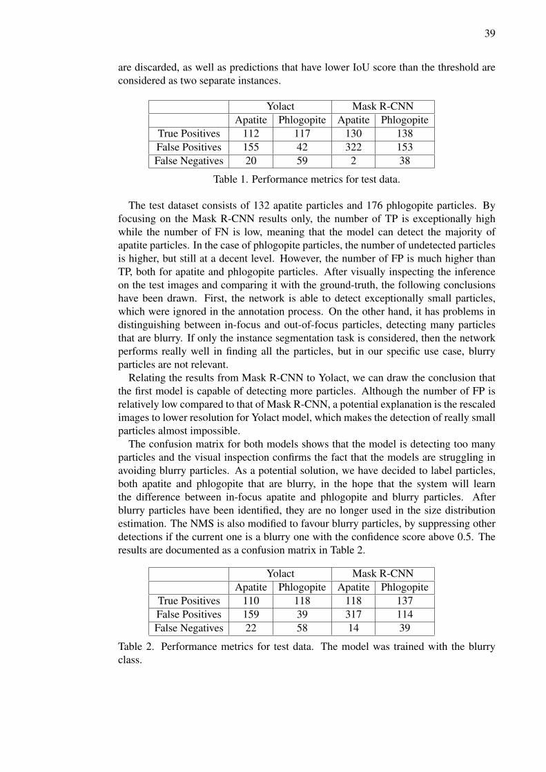
39
are discarded, as well as predictions that have lower IoU score than the threshold are
considered as two separate instances.
Yolact Mask R-CNN
Apatite Phlogopite Apatite Phlogopite
True Positives 112 117 130 138
False Positives 155 42 322 153
False Negatives 20 59 2 38
Table 1. Performance metrics for test data.
The test dataset consists of 132 apatite particles and 176 phlogopite particles. By
focusing on the Mask R-CNN results only, the number of TP is exceptionally high
while the number of FN is low, meaning that the model can detect the majority of
apatite particles. In the case of phlogopite particles, the number of undetected particles
is higher, but still at a decent level. However, the number of FP is much higher than
TP, both for apatite and phlogopite particles. After visually inspecting the inference
on the test images and comparing it with the ground-truth, the following conclusions
have been drawn. First, the network is able to detect exceptionally small particles,
which were ignored in the annotation process. On the other hand, it has problems in
distinguishing between in-focus and out-of-focus particles, detecting many particles
that are blurry. If only the instance segmentation task is considered, then the network
performs really well in finding all the particles, but in our specific use case, blurry
particles are not relevant.
Relating the results from Mask R-CNN to Yolact, we can draw the conclusion that
the first model is capable of detecting more particles. Although the number of FP is
relatively low compared to that of Mask R-CNN, a potential explanation is the rescaled
images to lower resolution for Yolact model, which makes the detection of really small
particles almost impossible.
The confusion matrix for both models shows that the model is detecting too many
particles and the visual inspection confirms the fact that the models are struggling in
avoiding blurry particles. As a potential solution, we have decided to label particles,
both apatite and phlogopite that are blurry, in the hope that the system will learn
the difference between in-focus apatite and phlogopite and blurry particles. After
blurry particles have been identified, they are no longer used in the size distribution
estimation. The NMS is also modified to favour blurry particles, by suppressing other
detections if the current one is a blurry one with the confidence score above 0.5. The
results are documented as a confusion matrix in Table 2.
Yolact Mask R-CNN
Apatite Phlogopite Apatite Phlogopite
True Positives 110 118 118 137
False Positives 159 39 317 114
False Negatives 22 58 14 39
Table 2. Performance metrics for test data. The model was trained with the blurry
class.

40
Despite lowering a bit the number of FP, there is an increase in FN. The same
applies for both architectures. Although the confusion matrix is a robust performance
measurement, one has to fix a confidence score threshold and an IoU score threshold,
which offers just a snapshot. Optimal thresholds can be chosen by applying a metric
that is based on varying these scores and assess how the model performs.
5.1.2. Precision-Recall Curve
Precision - Recall measure (PR) is a useful performance measure when the classes are
imbalanced and when the main objective is to find a trade-off between parameters.
Precision represents the rate of FP, while recall represents the rate of FN. They can be
mathematically formulated as:
P =TP
TP + FP
R =TP
TP + FN
We can assess the performance of the model by visually inspecting the area under
the PR curve. A high area indicates high precision and high recall, meaning low FP
and FN rates. A system with high precision, but low recall returns few results, but most
of them are correct. On the other hand, a system with high recall, but low precision
returns many results, but most of them are incorrect. The ideal system has both high
precision and recall, but in real-world scenarios, we have to aim for a trade-off between
these two, depending on the use-case of the system.
Figure 22 shows a comparison of PR curves between two models, both trained on
Mask R-CNN architecture, but one has been trained with an additional blurry class for
blurry particles. On the same figure, the IoU score threshold is varied and different
confidence scores are highlighted.

41
(a) Model trained with two classes: apatite and
phlogopite
(b) Model trained with three classes: apatite,
phlogopite and blurry particle
Figure 22. Precision-Recall curve for test set using Mask R-CNN.
Following the same procedure, we compute the PR curves for the Yolact model,
trained with and without the blurry particle class. Figure 23 shows the obtained results.
For Yolact, it is obvious that the addition of the third class, blurry particle, results in
an improved precision and recall. To achieve a trade-off between precision and recall,
the best configuration would be an IoU score of 0.5 and a confidence score of 0.5.
Depending on the specificity or sensitivity requirements, different configurations can
be selected. Unexpectedly, for certain configurations, the Yolact model proves to work
even better than the Mask R-CNN, precisely in terms of precision, since Yolact is much
less likely to predict false positives.
(a) Model trained with two classes (b) Model trained with three classes
Figure 23. Precision - Recall curve for the test set using Yolact model.

42
Mean average Precision
Most of the time though, expressing the overall performance in just a number is
desired due to its simplicity and ease of understanding. The Average Precision (AP)
represents one of the most used metric for assessing a DL model in the task of instance
segmentation. The AP is defined as the area under the PR curve.
AP =
∫
1
0
p(r)dr
As a pre-processing step, usually the PR curve has a zig-zag pattern and needs to
be smoothed out. This is done by replacing each precision value with the maximum
precision value to the right of that recall score. Then, an interpolation is performed
to get the final result. In COCO, a 101-point interpolation is performed on the PR
curve. Traditionally, AP is performed across a range of IoU thresholds (0.5-0.95). The
mean Average Precision (mAP) is the average of AP’s calculated at all IoU thresholds
between 0.5 and 0.95, for all classes.
5.1.3. Inference Time
To have a complete analysis of the two DNN architectures applied for this use case,
a comparison in terms of processing speed must be performed. Both architectures
had a ResNet 101 backbone. Regarding image size, Mask R-CNN was trained with
2048x2048 images, while for Yolact, images had to be resized to 550x550, which
resulted in slight accuracy loss, but gained significant processing time. Even if the
input image size differs, according to [43], Yolact is supposed to be faster than Mask
R-CNN. In our experiments, inferencing on a sample of images resulted in 23 FPS
processing speed for Yolact and only 5 FPS for Mask R-CNN. The requirement for
online grinding control and monitoring is a processing time of at least 10 FPS.
5.2. Size Distribution
All the evaluated metrics above rely on one essential concept: having a reliable,
fixed ground-truth. As it was specified in Section 4.3.1, the annotation process is
not straightforward and can suffer from errors due to the highly specialized domain.
Because of this, it is mandatory to evaluate our models with respect to a reference
measurement, which does not rely on manual annotation. Outotec provided reference
measurements by operating the PSI 500. Figure 24 depicts the size distributions
for different datasets, by applying the laser diffraction method. Due to the inherent
inability of laser diffraction to distinguish between particles of different classes, the
DL-based pipeline must also combine the size distributions obtained from the apatite
and phlogopite particles in a mixed distribution, for achieving a correct comparison.

43
Figure 24. Reference measurements provided by Outotec’s PSI 500, using laser
diffraction technology.
Figure 25 shows the PSD of all samples, when Mask R-CNN model has been used, in
two formats: histogram and kernel density estimation (KDE). The process of obtaining
a histogram for a specific dataset is presented in Section 4.5. The same process
is applied for all samples and each histogram is normalized individually. However,
plotting all histograms on the same canvas leads to cluttered areas, from which it can
be hard to analyse the result. Additionally, due to the frequent spikes in the histograms,
a smooth curve that approximates the underlying distributions would be desirable. This
can be achieved by calculating the KDE for each sample, which replaces the discrete
histogram with a continuous, smooth curve that characterizes the observed PSD. It
can also introduce potential distortions, if the underlying data is not smooth enough or
bounded, but choosing a good set of smoothing parameters can alleviate this problem.
The computation of KDE was performed with the help of Seaborn [60], a Python data
visualization library, that uses only Gaussian kernels. The final curves are plotted on a
logarithmic scale, so that the axes match with the reference measurement.
When comparing the reference PSD with the ones obtained by our method, we have
to take into consideration certain aspects. First, the laser diffraction method is capable
of measuring only particles of up to 1 mm, which translates to approximately 286
pixels. By referring to Section 4.3.2 and Figure 19, the imaging system is capable
of detecting larger particles, hence the size distribution might vary from the reference
measurement. Second, after a visual inspection of the datasets, it was observed that a
significant number of medium-large particles, usually phlogopite, are out-of-focus, due
to the narrow depth-of-field. Hence, there is a strong possibility that such particles are
measured by the laser diffraction, but for the current imaging system it is impossible
to correctly process them.
Analysing Figure 25 and Figure 24, it seems like sample4 and sample5 still have
the highest magnitude and sample1, sample2 and sample3 follow the trend of two
spikes, although the magnitude is reversed. Comparing the positions of distributions,
DL-based system detects particles that are smaller than particles detected by the laser
diffraction. Surprisingly, the PSD obtained when applying Yolact indicates different
distributions. Corroborating the shape and position of the PSD curves with confusion
matrix and with the limitation of Yolact processing only 550x550 images, it becomes

44
clear that Yolact model is having difficulties in detecting smaller particles. The shapes
of PSD curves are tighter than that of the ones obtained with Mask R-CNN, while the
peaks are slightly shifted to the left.
(a) Histogram of particle size (b) Kernel density estimation for the PSD
Figure 25. PSD estimated by Mask R-CNN model trained with blurry labelled
particles.
(a) Histogram of particle size (b) Kernel density estimation for the PSD
Figure 26. PSD estimated by Yolact model trained with blurry labelled particles.
To better understand the impact of each model on the PSD, Figure 27 shows the
ground-truth PSD compared to the PSD obtained by the two models. The graph
supports the hypothesis that Mask R-CNN is more biased towards detecting small,
blurry particles than Yolact is. Furthermore, the inference PSD results validate that DL
models can successfully segment instances of particles and produce PSDs similar to
the ground-truth. We have also analysed the PSD of apatite and phlogopite individually
by plotting the graph in Figure 28, and the same conclusion was reached, that small
apatite particles are detected by the Mask R-CNN. Regarding phlogopite, the PSDs
look more similar and closer to the ground-truth, since they are easier to segment.
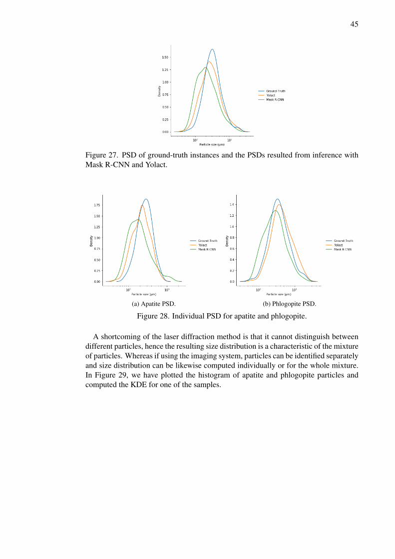
45
Figure 27. PSD of ground-truth instances and the PSDs resulted from inference with
Mask R-CNN and Yolact.
(a) Apatite PSD. (b) Phlogopite PSD.
Figure 28. Individual PSD for apatite and phlogopite.
A shortcoming of the laser diffraction method is that it cannot distinguish between
different particles, hence the resulting size distribution is a characteristic of the mixture
of particles. Whereas if using the imaging system, particles can be identified separately
and size distribution can be likewise computed individually or for the whole mixture.
In Figure 29, we have plotted the histogram of apatite and phlogopite particles and
computed the KDE for one of the samples.

46
(a) (b)
Figure 29. Histogram and KDE for apatite and phlogopite particles of sample 1.
47
6. DISCUSSION
This work investigates the application of DL-based instance segmentation in the
context of estimating PSD. To achieve this goal, two DNNs, specialised for the
task of instance segmentation, have been trained with images of particles in fluid
suspension. The first architecture to be tested was Mask R-CNN, a robust and powerful
architecture, especially suited for transfer learning. Although the model yielded
good results on our dataset, the major drawback was the slow processing time and
considering the purpose of the overall system, which is real-time particle monitoring,
we had to shift the focus towards an architecture more specialized in real-time
processing. Yolact is designed to be a simple, lightweight, real-time DNN for instance
segmentation, while maintaining a high level of accuracy. An extensive comparison
was performed between the two models to understand the key differences and to obtain
an optimal trade-off between accuracy and speed, so that the requirements for an online
particle monitoring system would be fulfilled. Moreover, the PSDs obtained from the
DL-based pipeline were compared to a reference measurement provided by the PSI
500 particle analyzer from Outotec, based on the laser diffraction principle. Despite
implementing a successful proof-of-concept, there are still a number of challenges
that need to be addressed in order to have a robust and reliable mechanism for PSD
estimation.
Inspired by the emerging concept of transfer learning, utilizing DNN for specialized
data and use cases seems like a promising idea. The known phrase that ’a DNN is as
good as the data you feed it’ has solid foundations and applies for each DL architecture.
Nevertheless, in specialized domains, good data is tremendously difficult to obtain and
even much harder it is to label it correctly and efficiently. Thanks to transfer learning,
we can utilize the general knowledge of a network to solve our particular task. This
results in significantly less labelled data and reduced training time. Transfer learning
represents the core concept of this work. The obtained results support the idea of
transferring knowledge, since the models are pre-trained on huge datasets containing
general objects and then the last layers of the models are fine-tuned for our specific
dataset.
Unfortunately, there is still a significant part of manual annotation involved. One
potential solution inspired from I. Yalniz et al. [61], would be to employ an iterative
pipeline that would expand the training set. In the beginning, few labelled instances
would be needed so that the system can be trained. Then, unlabelled data would be
fed to the network and only predictions that have a high confidence score would be
retained. Next, we would use the new labelled data by our model to expand the training
set and we would re-train the model, with the purpose of achieving better accuracy.
There are few investigations of how such frameworks would work, but it seems like a
promising new concept.
The dataset proved to be complex and required careful analysis. Blurriness has
also been a major challenge when carrying out the experiments. First, it is hard to
distinguish between an in-focus and out-of-focus particle, especially because of the
slurry composition that surrounds the particles. Apatite particles are significantly more
difficult to recognize as blurry due to their transparent nature. Second, some particles,
especially the large ones, are big enough to be partly in-focus and blurry at the same
time. This is caused by the narrow depth-of-field, resulting in possible inaccurate

48
measurements if such particles are considered. It is also not clear yet if the DNNs can
learn to distinguish between blurry and in-focus particles. The results obtained from
training with a blurry class support the idea that the DNN is capable of identifying
some of the blurry particles, but it is not yet robust enough. It may be that the network
has to be modified in order to also calculate a blurriness measure and to be part of the
learning and inference process, rather than a post-processing step, so that the impact on
the inference time is not significant. Moreover, comparing the PSDs from the PSI 500
with the ones obtained from the imaging system can be almost impossible, as the laser
diffraction can take into account also the blurry particles. Another observation resulted
from the annotation process was that some particles can be also mixed, consisting
of both apatite and phlogopite. Also, some cases were extremely hard to manually
annotate, namely attributing a class, due to increased similarity in particles. In turn,
this can affect the evaluation, as annotation is biased by the human annotator, especially
if he or she is not an expert in the mining field.
To overcome the detection of small particles in the case of Yolact, a possible solution
is to partition the original sized image, for example in four equal patches, then run
inference on each of them individually and in the last step, assemble the final picture.
The complex part lies in stitching back the four patches and solving the case of particles
that are split between the patches. Naturally, this operation would add an overhead for
the processing time, but may increase the number of small detected particles.
An experiment utilizing controlled particle size distributions obtained by sieving
enriched material was planned to strengthen the evaluation part of this thesis.
This would have allowed further analysing the performance of the approach. The
experiment would have been conducted first with pure apatite, allowing analysing
multiple distributions and directly comparing to the laser diffraction result. Then,
material from the same distribution would have been mixed with phlogopite to evaluate
the capability in a real scenario. Unfortunately, because of bad circumstances leading
to delays in the project, such an experiment was not feasible anymore.
There are still areas that need further research in order to apply DNNs to real-world,
hard engineering problems, but as the work performed up to this point shows, the trend
looks promising.

49
7. CONCLUSION
The principal objective of this thesis was the study of DL-based instance segmentation
for obtaining the PSD. Obtaining the PSD in real-time serves for control and monitor
processes in the grinding circuit. The dataset comprised of images containing apatite
and phlogopite particles in fluid suspension, captured by a color camera. The particles
had to be identified in images and for that, two DNN models, specialized for the task
of instance segmentation, were trained and used for inference on the unlabeled data.
Once the particles have been identified, the PSD can be easily computed.
In contrast to other works [7], not only testing, but also validation and training
is performed on real-world data by leveraging the concept of transfer learning. No
synthetic data is generated and the data is manually annotated, taking in consideration
difficult cases where particles are mixed, partially blurred or overlapping with other
particles. The first trained architecture was Mask R-CNN, which provided exceptional
results, unfortunately being too slow for real-time processing. The focus was shifted
towards Yolact, a DNN designed with real-time performance in mind. In agreement
with the author’s claims, the results of applying Yolact confirmed both the real-
time processing and high accuracy, by achieving more than 20 FPS and comparable
accuracy to Mask R-CNN. Although a reference PSD was provided, the measurement
mechanism relies on laser diffraction, which operates entirely different and comparing
with the PSD obtained with the imaging system can be really difficult.
However, a key advantage of the image-based system, corroborated with the high
precision and real-time processing of the DNN, consists of computing a separate PSD
for each particle of interest. In our case, the apatite PSD is of utmost importance
and the proposed system is capable of completing this task. Moreover, it is capable
of distinguishing between blurry and in-focus particles and even detect overlapped
particles. The potential of using DNN in PSD estimation still needs to be explored and
refined further. Furthermore, limiting the amount of manual annotation is one of the
biggest challenge and this will be the focus of our future research.
50
8. REFERENCES
[1] Wills B.A. & Finch J.A. (2016) In: Wills’ Mineral Processing Technology
(Eighth Edition), Butterworth-Heinemann, Boston, pp. 147 – 179. URL:
http://www.sciencedirect.com/science/article/pii/
B9780080970530000078.
[2] Farzanegan A. & Vahidipour S. (2009) Optimization of comminution circuit
simulations based on genetic algorithms search method. Minerals Engineering
- MINER ENG 22, pp. 719 – 726. URL: http://www.sciencedirect.
com/science/article/pii/S0892687509000533.
[3] Advanced grinding circuit control using online analyzer systems. URL: https:
//www.outotec.com/products-and-services/newsletters/
minerva/minerva-issue-3--2016/adcanced-grinding-
circuit-control-using-online-analyzer-systems/.
[4] Mahony N.O., Campbell S., Carvalho A., Harapanahalli S., Velasco-Hernández
G.A., Krpalkova L., Riordan D. & Walsh J. (2019) Deep learning vs. traditional
computer vision. CoRR abs/1910.13796. URL: http://arxiv.org/abs/
1910.13796.
[5] Ye Z., Jiang X. & Wang Z. (2012) Measurements of particle size distribution
based on mie scattering theory and markov chain inversion algorithm. Journal of
Software 7.
[6] Kongas M., Saloheimo K., Pekkarinen H. & Turunen J. (2003) New particle size
analysis system for mineral slurries. IFAC Proceedings Volumes 36, pp. 309–314.
[7] Frei M. & Kruis F. (2020) Image-based size analysis of agglomerated
and partially sintered particles via convolutional neural networks. Powder
Technology 360, pp. 324 – 336. URL: http://www.sciencedirect.
com/science/article/pii/S003259101930854X.
[8] Wu Y., Wang W., Zhang F., Xiao Z., Wu J. & Geng L. (2018) Nanoparticle
size measurement method based on improved watershed segmentation. In:
Proceedings of the 2018 International Conference on Electronics and Electrical
Engineering Technology, EEET ’18, Association for Computing Machinery,
New York, NY, USA, p. 232 – 237. URL: https://doi.org/10.1145/
3277453.3286087.
[9] Park C., Huang J., Ji J. & Ding Y. (2012) Segmentation, inference, and
classification of partially overlapping nanoparticles. IEEE Transactions on
Pattern Analysis and Machine Intelligence 35.
[10] Yuanxin Zhu, Carragher B., Mouche F. & Potter C.S. (2003) Automatic particle
detection through efficient hough transforms. IEEE Transactions on Medical
Imaging 22, pp. 1053–1062.
51
[11] Frei M. & Kruis F.E. (2018) Fully automated primary particle size
analysis of agglomerates on transmission electron microscopy images via
artificial neural networks. Powder Technology 332, pp. 120 – 130.
URL: http://www.sciencedirect.com/science/article/pii/
S0032591018302249.
[12] Rossetti D., Squartini S. & Collura S. (2016) Machine learning techniques for
the estimation of particle size distribution in industrial plants. In: Advances in
Neural Networks, Springer International Publishing, Cham, pp. 335–343.
[13] Hussain R., Noyan M., Woyessa G., Retamal Marín R., Martinez P., Mahdi F.,
Finazzi V., Hazlehurst T., Hunter T., Coll T., Stintz M., Muller F., Chalkias G. &
Pruneri V. (2020) An ultra-compact particle size analyser using a CMOS image
sensor and machine learning. Light: Science & Applications 9.
[14] Krizhevsky A., Sutskever I. & Hinton G.E. (2012) Imagenet classification with
deep convolutional neural networks. In: Proceedings of the 25th International
Conference on Neural Information Processing Systems - Volume 1, NIPS’12,
Curran Associates Inc., Red Hook, NY, USA, p. 1097–1105.
[15] Russakovsky O., Deng J., Su H., Krause J., Satheesh S., Ma S., Huang Z.,
Karpathy A., Khosla A., Bernstein M., Berg A.C. & Fei-Fei L. (2015) ImageNet
Large Scale Visual Recognition Challenge. International Journal of Computer
Vision (IJCV) 115, pp. 211–252.
[16] Tzirakis P., Zhang J. & Schuller B.W. (2018) End-to-end speech emotion
recognition using deep neural networks. In: 2018 IEEE International Conference
on Acoustics, Speech and Signal Processing (ICASSP), pp. 5089–5093.
[17] Collobert R. & Weston J. (2008) A unified architecture for natural language
processing: Deep neural networks with multitask learning. In: Proceedings of
the 25th International Conference on Machine Learning, ICML ’08, Association
for Computing Machinery, New York, NY, USA, p. 160–167. URL: https:
//doi.org/10.1145/1390156.1390177.
[18] Miclea V. & Nedevschi S. (2018) Real-time semantic segmentation-based depth
upsampling using deep learning. In: 2018 IEEE Intelligent Vehicles Symposium
(IV), pp. 300–306.
[19] Simonyan K. & Zisserman A. (2014) Very deep convolutional networks for large-
scale image recognition. arXiv 1409.1556 .
[20] Szegedy C., Vanhoucke V., Ioffe S., Shlens J. & Wojna Z. (2016) Rethinking
the inception architecture for computer vision. In: 2016 IEEE Conference on
Computer Vision and Pattern Recognition (CVPR), pp. 2818–2826.
[21] Gonzalez R.C. & Woods R.E. (2006) Digital Image Processing (3rd Edition).
Prentice-Hall, Inc., USA.

52
[22] Lin M., Chen Q. & Yan S. (2014) Network in network. In: Y. Bengio & Y. LeCun
(eds.) 2nd International Conference on Learning Representations, ICLR 2014,
Banff, AB, Canada, April 14-16, 2014, Conference Track Proceedings. URL:
http://arxiv.org/abs/1312.4400.
[23] Springenberg J.T., Dosovitskiy A., Brox T. & Riedmiller M.A. (2015) Striving
for simplicity: The all convolutional net. In: Y. Bengio & Y. LeCun (eds.)
3rd International Conference on Learning Representations, ICLR 2015, San
Diego, CA, USA, May 7-9, 2015, Workshop Track Proceedings. URL: http:
//arxiv.org/abs/1412.6806.
[24] Ponti M.A., Ribeiro L.S.F., Nazare T.S., Bui T. & Collomosse J. (2017)
Everything you wanted to know about deep learning for computer vision but
were afraid to ask. In: 2017 30th SIBGRAPI Conference on Graphics, Patterns
and Images Tutorials (SIBGRAPI-T), pp. 17–41.
[25] Bengio Y., Simard P. & Frasconi P. (1994) Learning long-term dependencies with
gradient descent is difficult. IEEE Transactions on Neural Networks 5, pp. 157–
166.
[26] Glorot X. & Bengio Y. (2010) Understanding the difficulty of training
deep feedforward neural networks. Journal of Machine Learning Research -
Proceedings Track 9, pp. 249–256.
[27] LeCun Y., Boser B., Denker J.S., Henderson D., Howard R.E., Hubbard W. &
Jackel L.D. (1989) Backpropagation applied to handwritten zip code recognition.
Neural Computation 1, pp. 541–551.
[28] Ioffe S. & Szegedy C. (2015) Batch normalization: Accelerating deep network
training by reducing internal covariate shift. In: F.R. Bach & D.M. Blei
(eds.) Proceedings of the 32nd International Conference on Machine Learning,
ICML 2015, Lille, France, 6-11 July 2015, JMLR Workshop and Conference
Proceedings, vol. 37, JMLR.org, JMLR Workshop and Conference Proceedings,
vol. 37, pp. 448–456. URL: http://proceedings.mlr.press/v37/
ioffe15.html.
[29] He K. & Sun J. (2015) Convolutional neural networks at constrained time cost.
In: IEEE Conference on Computer Vision and Pattern Recognition, CVPR 2015,
Boston, MA, USA, June 7-12, 2015, IEEE Computer Society, pp. 5353–5360.
URL: https://doi.org/10.1109/CVPR.2015.7299173.
[30] He K., Zhang X., Ren S. & Sun J. (2016) Deep residual learning for image
recognition. In: 2016 IEEE Conference on Computer Vision and Pattern
Recognition (CVPR), pp. 770–778.
[31] Adelson E.H., Anderson C.H., Bergen J.R., Burt P.J. & Ogden J.M. (1984)
Pyramid methods in image processing. RCA Engineer 29, pp. 33–41.
[32] Lin T., Dollár P., Girshick R., He K., Hariharan B. & Belongie S. (2017) Feature
pyramid networks for object detection. In: 2017 IEEE Conference on Computer
Vision and Pattern Recognition (CVPR), pp. 936–944.

53
[33] Girshick R., Donahue J., Darrell T. & Malik J. (2016) Region-based
convolutional networks for accurate object detection and segmentation. IEEE
Transactions on Pattern Analysis and Machine Intelligence 38, pp. 142–158.
[34] Uijlings J., Sande K., Gevers T. & Smeulders A. (2013) Selective search for
object recognition. International Journal of Computer Vision 104, pp. 154–171.
[35] Girshick R. (2015) Fast R-CNN. In: 2015 IEEE International Conference on
Computer Vision (ICCV), pp. 1440–1448.
[36] He K., Zhang X., Ren S. & Sun J. (2015) Spatial pyramid pooling in deep
convolutional networks for visual recognition. IEEE Transactions on Pattern
Analysis and Machine Intelligence 37, pp. 1904–1916.
[37] Ren S., He K., Girshick R. & Sun J. (2017) Faster R-CNN: Towards Real-Time
Object Detection with Region Proposal Networks. IEEE Transactions on Pattern
Analysis and Machine Intelligence 39, pp. 1137–1149.
[38] He K., Gkioxari G., Dollár P. & Girshick R. (2017) Mask R-CNN. In: 2017 IEEE
International Conference on Computer Vision (ICCV), pp. 2980–2988.
[39] Long J., Shelhamer E. & Darrell T. (2015) Fully convolutional networks for
semantic segmentation. In: 2015 IEEE Conference on Computer Vision and
Pattern Recognition (CVPR), pp. 3431–3440.
[40] Xie S., Girshick R., Dollár P., Tu Z. & He K. (2017) Aggregated residual
transformations for deep neural networks. In: 2017 IEEE Conference on
Computer Vision and Pattern Recognition (CVPR), pp. 5987–5995.
[41] Huang Z., Huang L., Gong Y., Huang C. & Wang X. (2019) Mask scoring r-cnn.
In: 2019 IEEE/CVF Conference on Computer Vision and Pattern Recognition
(CVPR), pp. 6402–6411.
[42] Lin T.Y., Maire M., Belongie S., Hays J., Perona P., Ramanan D., Dollár P. &
Zitnick C.L. (2014) Microsoft COCO: Common Objects in Context. In: D. Fleet,
T. Pajdla, B. Schiele & T. Tuytelaars (eds.) Computer Vision – ECCV 2014,
Springer International Publishing, Cham, pp. 740–755.
[43] Bolya D., Zhou C., Xiao F. & Lee Y.J. (2019) Yolact: Real-time instance
segmentation. In: 2019 IEEE/CVF International Conference on Computer Vision
(ICCV), pp. 9156–9165.
[44] Bordignon F., Figueiredo L., Exterkoetter R., Rodrigues B. & Duarte M. (2019)
Deep learning for grain size and porosity distributions estimation on micro-
ct images. Proceedings of the 16th International Congress of the Brazilian
Geophysical Society & Expogef , pp. 1–6.
[45] Ji S., Xu W., Yang M. & Yu K. (2013) 3d convolutional neural networks for
human action recognition. IEEE Transactions on Pattern Analysis and Machine
Intelligence 35, pp. 221–231.

54
[46] Zhang J., Zihao W., Chen Y., Han R., Liu Z., Sun F. & Zhang F. (2019) PIXER:
An automated particle-selection method based on segmentation using a deep
neural network. BMC Bioinformatics 20.
[47] Chen L., Papandreou G., Kokkinos I., Murphy K. & Yuille A.L. (2018)
DeepLab: Semantic Image Segmentation with Deep Convolutional Nets, Atrous
Convolution, and Fully Connected CRFs. IEEE Transactions on Pattern Analysis
and Machine Intelligence 40, pp. 834–848.
[48] Xiao Y. & Yang G. (2017) A fast method for particle picking in cryo-
electron micrographs based on fast r-cnn. APPLIED MATHEMATICS AND
COMPUTER SCIENCE: Proceedings of the 1st International Conference on
Applied Mathematics and Computer Science 1836.
[49] Wang F., Gong H., Liu G., Li M., Yan C., Xia T., Li X. & Zeng J.
(2016) DeepPicker: A deep learning approach for fully automated particle
picking in cryo-EM. Journal of Structural Biology 195, pp. 325 – 336.
URL: http://www.sciencedirect.com/science/article/pii/
S1047847716301472.
[50] Abdulla W. (2017), Mask R-CNN for object detection and instance segmentation
on Keras and TensorFlow. https://github.com/matterport/Mask_
RCNN.
[51] Cordts M., Omran M., Ramos S., Rehfeld T., Enzweiler M., Benenson R., Franke
U., Roth S. & Schiele B. (2016) The cityscapes dataset for semantic urban
scene understanding. In: 2016 IEEE Conference on Computer Vision and Pattern
Recognition (CVPR), pp. 3213–3223.
[52] Dutta A. & Zisserman A. (2019) The VIA Annotation Software for Images,
Audio and Video. In: Proceedings of the 27th ACM International Conference
on Multimedia, MM ’19, Association for Computing Machinery, New York,
NY, USA, p. 2276–2279. URL: https://doi.org/10.1145/3343031.
3350535.
[53] Shao L., Zhu F. & Li X. (2015) Transfer learning for visual categorization: A
survey. IEEE Transactions on Neural Networks and Learning Systems 26, pp.
1019–1034.
[54] Zamir A.R., Sax A., Shen W., Guibas L., Malik J. & Savarese S. (2018)
Taskonomy: Disentangling task transfer learning. In: 2018 IEEE/CVF
Conference on Computer Vision and Pattern Recognition, pp. 3712–3722.
[55] Shorten C. & Khoshgoftaar T. (2019) A survey on image data augmentation for
deep learning. Journal of Big Data 6.
[56] Prechelt L. (1996) Early stopping-but when? In: G.B. Orr & K. Müller (eds.)
Neural Networks: Tricks of the Trade, Lecture Notes in Computer Science, vol.
1524, Springer, pp. 55–69. URL: https://doi.org/10.1007/3-540-
49430-8_3.

55
[57] Biewald L. (2020), Experiment tracking with weights and biases. URL: https:
//www.wandb.com/.
[58] Shanthi C., Porpatham R. & Pappa N. (2014) Image analysis for particle size
distribution. International Journal of Engineering and Technology 6, pp. 1340–
1345.
[59] Everingham M., Gool L., Williams C.K., Winn J. & Zisserman A. (2010) The
Pascal Visual Object Classes (VOC) Challenge. Int. J. Comput. Vision 88, p.
303–338. URL: https://doi.org/10.1007/s11263-009-0275-4.
[60] Waskom M., Botvinnik O., O’Kane D., Hobson P., Lukauskas S., Gemperline
D.C., Augspurger T., Halchenko Y., Cole J.B., Warmenhoven J., de Ruiter J.,
Pye C., Hoyer S., Vanderplas J., Villalba S., Kunter G., Quintero E., Bachant
P., Martin M., Meyer K., Miles A., Ram Y., Yarkoni T., Williams M.L.,
Evans C., Fitzgerald C., Brian, Fonnesbeck C., Lee A. & Qalieh A. (2017),
mwaskom/seaborn: v0.8.1 (september 2017). URL: https://doi.org/10.
5281/zenodo.883859.
[61] Yalniz I.Z., Jégou H., Chen K., Paluri M. & Mahajan D. (2019), Billion-scale
semi-supervised learning for image classification.