Particle Swarm Optimization

Based Diophantine Equation

Solver

Siby Abraham* Department of Mathematics & Statistics, G.N. Khalsa College,

University of Mumbai, Mumbai-400019, India

E-mail: sibyam@gmail.com

*Corresponding author

Sugata Sanyal School of Technology & Computer Science

Tata Institute of Fundamental Research, Mumbai, India

Homi Bhabha Road, Mumbai-400005, India

E-mail: sanyal@tifr.res.in

Mukund Sanglikar Department of Mathematics, Mithibai College, Vile Parle (W),

University of Mumbai, Mumbai-400056, India.

Email: masanglikar@rediffmail.com.

Abstract: The paper introduces particle swarm optimization as a viable strategy to find numerical solution of Diophantine equation, for which there exists no general method of finding solutions. The proposed methodology uses a population of integer particles. The candidate solutions in the feasible space are optimised to have better positions through particle best and global best positions. The methodology, which follows fully connected neighbourhood topology, can offer many solutions of such equations.

Keywords: Diophantine equation, particle swarm optimisation, fitness function, position, velocity, learning factor, socio-cognitive coefficients, Fermat’s equation, elliptic curve.

Reference to this paper should be made as follows: Abraham, S (20--) ‘Particle Swarm Optimization based Diophantine Equation Solver, International Journal Bioinspired Computing Vol. ---, Nos. ----, pp.----

Biographical notes: Siby Abraham is an Associate Professor and Head, Department of Mathematics & Statistics at Guru Nanak Khalsa College, University of Mumbai. He is also a visiting faculty to Department of Computer Science, University of Mumbai, India. He received his PhD in Computer Science from University of Mumbai and MSc in Mathematics from Cochin University of Science & Technology, India. His current research interests include computational intelligence, nature and bio inspired computing.

Sugata Sanyal is a Professor at the School of Technology & Comp Sc at Tata Institute of Fundamental Research (TIFR), India. He received his PhD from TIFR under Mumbai University, M Tech from IIT, Kharagpur and B E from Jadavpur University, India. He was a visiting professor in the University of Cincinnati, USA. He is in the editorial board of three international journals. His current research interests include security in wireless and mobile ad hoc networks, distributed processing scheduling techniques and bio inspired computing.

Mukund Sanglikar is presently with the Department of Mathematics, Mithibai College, Mumbai, India. He is former Professor and Head of the Department of Computer Science, University of Mumbai, India. He was also the Chairman, Board of Studies in Comp Sc & IT and a member of Academic Council, University of Mumbai. He received his PhD in Computer Science and MSc in Mathematics from University of Mumbai, India. His current research interests include soft computing, networking, software engineering and mobile databases.

1 INTRODUCTION

A Diophantine Equation (Cohen 2007) (Rossen 1987)

(Zuckerman 1980) is a polynomial equation, given by

f(a1,a2,…..,an,x1,x2,……,xn) = N (1)

where ai and N are integers. Diophantine equations obtained

its name from third century BC Alexandrian Mathematician

Diophantus, who studied these equations in detail

(Bashmakova 1997). In his work ‘Arithmetic’, a treatise of

thirteen books, he asked for solutions for about 150 algebraic problems. These problems are now collectively

referred as Diophantine equations. Diophantine equations and its particular cases have

always been of great interest to Mathematicians (Bag 1979).

One of the simplest forms of such equations is given by

ax1 + bx2 = c (2)

If c is the greatest common divisor of ‘a’ and ‘b’

(i.e. c = (a, b)), then this equation has infinitely many

solutions, which can be obtained by extended Euclidian

Algorithm.

The equations given by

x1 n + x2

n = x3

n (3)

are of great significance. For n=1, the equation (3) has

infinitely many solutions. For n=2 also, the equation

provides infinitely many solutions. Such solutions, which

are called Pythagorean triplets, form sides of a right angled

triangle.

The French Mathematician Pierre de Fermat’s name is

the most relevant in the discussion of Equation (3). Fermat,

who died in 1665, had the habit of writing small notes on

the margins of the book he read. In one of such notes made

on the Latin translation of Diophantus’ ‘Arithmetic’ by

Backet, he wrote that the equation (3) has no solutions for

n>2. The notes appeared alongside problem 8 in Book II of

‘Arithmetic’ says “ …given a number which is square, write

it as a sum of two other squares”. Fermat’s note further

stated that “on the other hand, it is impossible for a cube to

be written as a sum of two cubes or a fourth power to be

written as sum of two fourth powers or, in general, for any

number which is a power greater than the second to be

written as a sum of two like powers? I have a truly

marvelous demonstration of this proposition which this

margin is too narrow to contain” (Shirali & Yogananda

2003). Since then, this conjecture is known as Fermat’s Last

Theorem (FLT), though there was no general proof of it

irrespective of the number of attempts to find one. Table 1

shows the important attempts by Mathematicians to prove

FLT for different cases (Edwards 1977). Finally, in 1994,

the British Mathematician Andrew Wiles presented a

sophisticated proof using elliptic curves for FLT and ended

the conjecture. Thus Fermat’s Last Theorem became a

theorem at last! (Shirali & Yogananda 2003)

An elliptic curve is a Diophantine equation (Stroeker

and Tzanakis 1994)(Poonan 2000) of the form

y 2

= x 3 + ax + b (4)

where a and b are rational and the cubic x 3 + ax + b has

distinct roots. Elliptic curves (Koblitz 1984) form a highly

advanced structure because of its mathematical rigor.

Table 1: Status of FLT for different cases

If P and Q are any two points on an elliptic curve, then we

can uniquely describe a third point which is the intersection

of the curve with the line through P and Q. The work of

Poincare showed that the points of E (real not just rational)

form an abelian group under a specific operation known as

chord-and-tangent addition with the ‘point at infinity’ O as

the identity element. Such Mathematical sophistication

makes elliptic curves a participant in high level applications.

For example, Elliptic curve based Public Key Cryptography

(Lin CH et al 1995)(Laih CS et al 1997) is quite effective as

discrete logarithmic problem on elliptic curve is tougher

than usual discrete logarithmic problems. Hence, such

systems require only shorter key size to have comparable

security offered by other public key cryptosystems.

Figure 1 Elliptic curves

Though there are different types of well known and

highly relevant Diophantine equations, the solutions of

which have always been surrounded by an air of enigma.

This is because a Diophantine Equation can have no

nontrivial solution, a finite number of solutions or an

infinite number of solutions. David Hilbert should be given

Year

Mathematician

Case proved

1640

Fermat

n=4

1770

Euler

n=3

1823 Sophie

Germaine

n=p, a prime known as Sophie

Germaine prime where 2p+1 is

also prime

1825

Dirichlet,

Legendre

n=5

1832

Dirichlet

n=14

1839

Lame

n=7

1847

Kummer

n=p, where p is a regular prime

the credit for giving a direction to the interest on

Diophantine equations and its solutions. In 2000, at the

second international conference of Mathematicians (Hilbert

1902), he asked “Given a Diophantine equation with any

number of unknowns and with rational integer coefficients:

devise a process, which could determine by a finite number

of operations whether the equation is solvable in rational

integers” as tenth of his famous twenty three problems.

Since then, the problem is known as Hilbert’s tenth problem

(Borowski et al 1991).

There have been many attempts to solve Hilbert’s tenth

problem. Davis et al (1982) showed that an algorithm to

determine the solvability of all exponential Diophantine

equations is impossible. Matiyasevich (1993) extended that

work by showing that there is no algorithm for determining

whether an arbitrary Diophantine equation has integral

solutions. This helped in ending the search of centuries for

finding a general method to solve a Diophantine equation.

This has not dampened the importance and interest on

Diophantine Equations and its solutions as newer and

modern application areas were added. These include Public

key cryptosystems (Laih CS 1997) (Lin CH 1995), Data

dependency in Super Computers (Tzen and Ni 1993) (Zhiyu

et al 1989), Integer factorization, Algebraic curves (Ponnen

2000), Projective curves (Brown & Myres 2002) (Stroeker

& Tzanakis 1994), Computable economics (Velu 2003) and

Theoretical Computer Science (Ibarra 2004) (Guarari 1982).

In this context, finding numerical solution to

Diophantine equations becomes important. However, this

turns out to be a tough problem to deal with primarily

because of the fact that the number of possible solutions

encountered is very huge. This means, following an

exhaustive, gradual and incremental method invite the

definite risk of computational complexity.

This paper introduces Particle Swarm optimization

(Eberhart et al 1995) (Kennedy et al 1995) as a meta-

heuristic search technique to find numerical solutions of

such equations. It shows how the socio psychological

behavior of custom made n-dimensional integer particles

effective in maneuvering the search space in finding a

solution to such equations. The paper discusses the

procedure which are validated using a class of Diophantine

equations given by

a1 . x1 p1 + a2 . x2

p2 + …….. + an . xn pn = N (5)

Other class of equations can also be tackled similar way.

The paper is organized as follows: Section 2 gives a

brief survey and discussion of related works. Section 3

explains the methodology used. Section 4 presents the

experimental results and section 5 deals with conclusion.

2 BRIEF SURVEY AND DISCUSSION

Since there exists no general method to find solution of a

Diophantine Equation, there have been few attempts to find

numerical solutions of it as the next possible way. However,

this turns out to be a tough problem to deal with as there are

Nn possible in the search space of (5). The search strategies

offered by Artificial Intelligence (AI) (Russell and Norwig

2003) (Luger 2006) could be possible alternatives because

of its flexibility to move around in the search space. Though

Breadth first search is guaranteed to find an optimal

solution, if it exists, the time and space complexities of

order O(bd+1) with branching factor ‘b’ and depth ‘d’,

discourage us to attempt it for larger equations. Depth first

search might blindly follow a branch of the search tree

without returning a solution. The other uninformed search

strategies like Depth Limited, Iterative Deepening and Bi-

directional also can come with similar handicaps. The

informed search technique Hill Climbing can get trapped in

local optimum points from where it finds it difficult to get

out. A* search was used by Abraham and Sanglikar (2009)

and found that the system runs out of space very fast.

There have been some attempts to apply soft computing

techniques to find numerical solution of (5). Abraham and

Sanglikar (2001) tried to find numerical solutions to such

Diophantine equations by applying genetic operators-

mutation and crossover Michalewich (1992). Though the

methodology could find solutions, it was not fully random

in nature and seemed more like a steepest ascent hill

climbing rather than a genetic algorithm. Hsiung and

Mathews (1999) tried to illustrate the basic concepts of a

genetic algorithm using first-degree linear Diophantine

equation given by a + 2b + 3c+ 4d = 30. Literature also

talks about an application of higher order Hopfield neural

network to find solution of Diophantine equation (Joya et al

1991). Abraham and Sanglikar (2007 a) explains the process

of avoiding premature converging points using ‘Host

Parasite Co-evolution’ (Hills 1992) (Paredis 1996)

(Wiegand 2003) in a typical GA. Later they used a method

involving evolutionary and co-evolutionary computing

(Rosin and Belew 1997) techniques (Abraham & Sanglikar

2007 b) to find numerical solutions to such equations. They

also used (Abraham & Sanglikar 2008) Simulated

Annealing as a viable probabilistic search strategy for

tackling the problem of finding numerical solution. These

methods, though effective to a certain extent for smaller

equations, are not good enough to deal with the

complexities of Diophantine equations.

3 SWARM-DOES METHODOLOGY

Though PSO algorithm is designed for real-value problems

(Shi 2004), there have been few attempts to apply them to

binary-value problems (Kennedy and Eberhart 1997)

(Agrafiotis and Cedeno 2002). This paper is an attempt to

apply the PSO methodology to integer value problems.

More importantly, this tries to apply the algorithm to a

Mathematical problem, an area which appears not so often

in the PSO literature.

The system developed to find numerical solution of

Diophantine equations using particle swarm optimization, is

called Particle Swarm Optimization based Diophantine

Equation Solver (SWARM-DOES). SWARM-DOES

attempts to apply PSO on the integer value problem of

finding integer solutions of (5). The particles are created as

integer particles to facilitate integer solutions. The

dimension of the particle depends upon the number of

variables of the equation under study. If an equation has n

variables, the dimension of the particle would also be ‘n’.

As in the other PSO systems, each particle is identified with

two factors: the velocity and position. The velocity factor

shows the measure of the movement of the particle and the

position conveys the current status of the particle. Each of

the particle tries to change its velocity and hence the

position. They move in the multidimensional space in a

collective fashion. The objective of the movement of these

particles is to find the best position a particle can have in

this multidimensional search space. The strategy involves

mimicking the best position it had and the best position

other particles have had till then.

3.1 Initial population

The procedure of finding numerical solution to (5) starts

with a population of random particles or swarms of fixed

size. The particles are constructed as integer particles based

on probable values of variables appearing in the equation

(5). The construction of these particles is facilitated by

incorporating knowledge of the domain and the constraints

the possible values face as solutions in the problem.

A possible solution of equation (5) can be

(s1, s2, ……, sn) where each si is an integer which lies

between the numbers 1 and the prth

power root of N, where

pr is the minimum value of p1, p2, …. and pn. Hence a

particle in the initial population is taken as an n-dimensional

vector (d1, d2, …….., dn) where each of the coordinate di

takes a random integer value between 1 and integer part of

N1/pr

. Thus, the initial population is a random collection of

fixed number of integer particles which occupy random

positions at the search space of candidate solutions of a

Diophantine equation. Initially, each of the particles is given

velocities zero. The population size can be chosen as any

relevant value.

3.2 Feasible space

SWARM-DOES procedure separates the positions a particle

occupies into two spaces: the feasible space and the non-

feasible space. The feasible space consists of all positions,

which a particle can fly legally without violating the

constraints of the problem. The non-feasible space consists

of all other positions of the particle. The feasible space X of

the equation (5) is defined as

X = {(d1, d2, …….., dn): di = 1, 2, 3,.... N1/pr

} (6)

where pr is given by

pr = minimum {p1, p2, …. , pn} (7)

Here p1, p2, …. , pn are the powers of the Diophantine

equation (5). This selection is based on the domain

knowledge that the equation (5) cannot have a solution

whose power is less than the prth

power root of N. Thus,

the problem of finding numerical solution of a Diophantine

equation is a constrained problem of finding numerical

solution of the equation (5) by searching within the feasible

space X. The proper selection of feasible space helps in

identifying to check whether a candidate solution satisfies

the constraints of the given problem. As shown in the next

section, the identification of candidates belonging to

feasible solution is made possible by introducing a domain

specific fitness function. The particle with a valid and

acceptable fitness function value only are allowed to be in

the feasible space. The candidates with invalid fitness

function are directed to belong to the infeasible space.

3.3 Fitness function

Fitness function value of a particle gives the effectiveness of

the particle in the search space. The fitness function of a

particle in SWARM DOES is defined as

fitness =Abs (N-(a1*x1

p1

+a2*x2

p2

+…+an*xn

pn

)) (8)

The value of the fitness function indicates the distance

between the current position of the particle and its solution.

If fitness=0 for a particle, then that position of the particle is

taken as a solution. At each iteration, the attempt is to

reduce this distance. Thus, the procedure becomes a

minimization process in which each of the particles tries to

reduce the distance between its present status and the

solution of the equation whose fitness function value is

given to be zero.

3.4 Selection of Pbest

The movement of a particle in the search space is guided by

the previous best experience of the particle and the best

experience encountered by all the particles till then. The

best position of a particle faced till then is called the ‘pbest’

of that particle. The ‘pbest’ acts as the memory of the

particle. Based on the best position encountered by that

particle during the exploration process, the particle tries to

mimic that best experience by duplicating the same. Thus,

each particle memorizes one best experience it encountered

till then and tries to optimize the current position by

comparing the best experience it had. The fitness function

value of a particle acts as a representative value in the

selection of ‘pbest’ of the particle at that iteration. A particle

with the lowest fitness function value is taken as the ‘pbest’

of the particle. Here the particle remembers only the states

which are feasible and discard the particles in the infeasible

space. It is possible that ‘pbest’ position of a particle may

survive for a longer time in the search procedure. Better the

value of the fitness of the ‘pbest’, higher the chance for the

particle to survive for a long time. In a highly matured run

of the process, ‘pbest’ values do not survive for a long time.

The dynamic movement of ‘pbest’ values shows the

effectiveness of convergence of the procedure. At the

beginning of the process, ‘pbest’ of each of the particle is

initialized to the initial fitness value of that particle.

3.5 Selection of gbest

The movement of a particle in the multidimensional search

space of a Diophantine equation also depends on the best

position encountered by all particles in the population till

then. This way, the flow of a particle is influenced by the

social environment in which it flows (Hu et al 2004). Each

of the particles tries to improve its position by comparing

the best position encountered by any particle till then during

the entire exploration process. This best position of all the

particles in the entire the search process is called the ‘gbest’.

Initially, the particle having the best fitness function value is

taken as the ‘gbest’. This is changed dynamically as the

process continues. This is made possible by having a

reference to the stored value of the ‘gbest’. This reference

is used to update the position and velocity of each of the

particle in the population. At any instant, the particle

changes its velocity by comparing the same with that of the

‘gbest’ particle. Hence the ‘gbest’ particle helps in updating

the position of each of the particle in the whole search

process.

3.6 Update of velocity

The movement of a particle xt at time t to that at time t+1 is

facilitated by updating the velocity and hence the position of

the particle. The velocity vt of the particle xt at time t is

updated using the formula

Vt+1 = c1v t+ c2.rand1().(xt – pbest) +

c3.rand2().(xt – gbest) (9)

where rand1() and rand2() are two random numbers

between 0 and 1. Since xt = (d1, d2, ……., dn), the updating

formula for the velocity for each coordinate of a particle is

given by

Vt+1(di) = c1vt(di)+c2.rand1().(xt(di)–pbestdi)+

c3.rand2().(xt(di)- gbestdi) (10)

The component (xt(di)–pbestdi) gives the difference of

the corresponding coordinates of the current position and

that of the ‘pbest’ position of the particle. c2 is a constant,

called the cognitive coefficient, denotes the trusts the

particle has on its own previous experience. Thus, the factor

rand1()(xt(di)–pbestdi) identifies the amount of change in

velocity of a particle due to its own previous experience.

The component (xt(di)- gbestdi) gives the difference of

the corresponding coordinates of the current position of the

particle and that of the ‘gbest’ position. The social

coefficient c3 quantifies the trusts the particle has on its own

neighbors. Hence, the factor c3.rand2().(xt(di)- gbestdi)

represents the amount of change in velocity of a particle due

to its neighbors.

3.7 Update of position

A particle changes its position using its updated velocity.

The following formula is used for this purpose:

xt+1 = x t + v t+1 (11)

Thus, the coordinates of the new position obtained by a

particle is given the formula

xt+1(d i) = x t (d i) + v t+1 (d i) (12)

Since the paper is interested only in non-negative solutions

of the given Diophantine equation, those values of Xt+1(di)

which belong to the non-feasible space are discarded. The

occurrence of positions belonging to non-feasible space

demands an automatic revision. This is facilitated by a

unique strategy in SWARM-DOES.

According to this, any particle which risks to flow into

the non-feasible space is brought back to the feasible space.

It has been observed that a particle in the procedure can fall

into the non-feasible space in two cases:

Case 1: When coordinate of any particle di < 0;

Case 2: di > particleRange, where

particleRange= N1/pr

(13)

In case 1, the particle is made to flow into the feasible space

by suitably redefining di as

di = (-1) * di (14)

In the case 2 also, the particle is forced to fly back to the

feasible space but using the instruction:

di = di % particleRange (15)

In either case, a particle is not allowed to fly into the non-

feasible space. This strategy of not allowing a particle the

risk of flying into the non-feasible space by forcefully

diverting its route is quite effective in managing the

constraints of the given Diophantine equation.

3.8 Neighbourhood topology

SWARM-DOES follow the fully connected neighborhood

topology (Sierra and Coello 2006), which is also called star

topology (Engelbrecht 2002), against local topologies. As

per this, each integer particle flies through the search space

by dynamically adjusting its position with respect to ‘pbest’

and ‘gbest’ (Kennedy 1999) (Kennedy et al 2001) (Kennedy

and Mendes 2002) (Shi 2004). Thus, the graph obtained to

show the connections between the particles is a fully

connected graph as shown in figure 2.The circle shows the

particles and the line segments show the connection. In such

a topology, all members of the swarm are connected to one

another. The adoption of this fully connected topology

against other popular topologies is deliberate. We felt that

the other topologies, by the virtue of guiding the search

process by focusing only on the best position encountered.

Figure 2 Fully connected graph

by the particles in a neighborhood topology, could converge

only slowly. On the other hand, the global version can

provide a faster convergence by focusing on the best

positions encountered by all particles by taking the whole

population as its neighbors. This is because, all the particles

receive information about the best position of the entire

swarm simultaneously and are better equipped to

incorporate this information

Having the complete population of particles as neighbors

brings a lot of convenience and effectiveness to the

procedure. The best experience encountered by any particle

can be shared by the other particles in this mechanism. This

makes the system much more responsive than other local

level topologies which focus only on a limited number of

neighbors in the topological vicinity of a particle.

3.9 Learning factors

As the equation (10) shows, SWARM-DOES incorporate

the velocity changes of a particle in three parts. As is the

popular convention, we call them momentum part, cognitive

part and social part. The momentum part corresponds to the

factor c1vt(di) of the equation (10). The constant c1, called

the inertia weight, balances the global exploration and local

exploitation of the search. It has been experimentally shown

that large inertia weight increases the global search while

the small value supports the local search (Shi 2004).

In equation (10), the factor c2(xt(di)–pbestdi) conveys the

coordinate wise effect of the current position of the particle

and the best position encountered by the particle till then.

The particle tries to optimize its performance by comparing

its best performance. This factor is enhanced using the

cognitive factor c2. On psychological terms, c2 shows the

tendency of the particle to duplicate the past best behavior.

The factor c3.rand2().(xt(di)- gbestdi) indicates the

quantity by which the velocity of a particle can change

based on the best performance of all particles till then. The

constant c3, called the social coefficient represent the

confidence with which a particle can follow the success of

other particles.

Since the effectiveness of the search process to a great

extend depends on the choice of the values of the values of

the constants c1, c2 and c3, we have taken care to select the

optimum values for these. After experimental results we

finalized the value of c1 as 1 and the values of c2 and c3 as 2

each. Though there have been many varied forms of inertia

weight (Shi and Eberhart 1998a, 1999) (Shi and Eberhart

2001a, 2001b) (Ratnaweera et al2004), SWARMDOES kept

the value of c1 as 1 deliberately. The possible effect of other

values of c1 is brought more effectively by incorporating a

clamp on the possible values of velocity as the section 3.10

demonstrates.

3.11 Maximum velocity

In order to restrict the change in velocity of a particle within

an acceptable range, a variable called Vmax is used. Using

this concept, the equation (10) is not given a free hand to

change the value of the velocity of a particle. However, the

values of the velocity are allowed to change only within an

acceptable range. It is facilitated using a specially defined

methodology. As per this, based on the value of

‘particleRange’ defined in equation (13), we define a new

variable maxRange as given below

maxRange=minimum {particleRange, 5} (16)

Then, the velocity coordinates are allowed to change only

within the ± maxRange. That means, the coordinates of the

velocity are allowed to change only within the region given

by

(-vmax, vmax) = (-maxRange, maxRange) (17)

In cases, where the velocity values go outsides this range,

the procedure brings them back to the feasible range by

using the mathematical equation

vt+1(di) = vt+1(di) % maxRange (18)

Having the restriction on the possible values of velocity

allows us to have a much thorough local search of the

search space.

3.11 Sequence of solutions

The SWARM-DOES procedure is run many times until get

a particle whose fitness value is zero or termination

condition is met. After getting one solution, the procedure

offers to continue further to get as many solutions of the

equation as possible. This requires some fine tuning in the

procedure explained until now. During experiment, it is

observed that after finding the first solution, the usual

procedure of updating ‘pbest’ and ‘gbest’ result in the

repetition of the same solution again and again. The system

overcomes this problem by replacing the particle, which

gives the solution, by a randomly generated new particle

with velocity assigned as zero. This would enable the

optimization to search another untried and untested domain.

Leaving an optimised region and charting an entirely new

untried and new region helps the procedure to find as many

numerical solutions as possible for a given Diophantine

equation.

3.12 Termination condition

The procedure is terminated when the number of

generations specified is completed. Or, alternatively, the

procedure halts when the system offers one solution asking

for the option of continuing the search to produce newer and

fresher solutions of the given equation. Here, one can

terminate the procedure if satisfied with one solution. The

option of offering newer solutions helps to find as many

numerical solutions as possible for a given Diophantine

equation. This is quite significant, in the light of the fact,

that there exists no general method even to find a single

solution. The system experienced the running of system up

to more than fifty thousand generations or iterations.

4 EVALUATION AND EXPERIMENTAL RESULTS

The SWARM-DOES strategy was validated by testing the

system with different types of equations. The different

classes of Diophantine equations given in (5) were tried by

supplying different number of variables and varied values of

degrees. These results also reveal some important

characteristics of swarm intelligence while finding the

solution of the given Diophantine equation. The important

features the results demonstrate include convergence

properties of the ‘pbest’ and ‘gbest’ particles, directed

random movement of the procedure during the search and

the random update of the values of velocity among others.

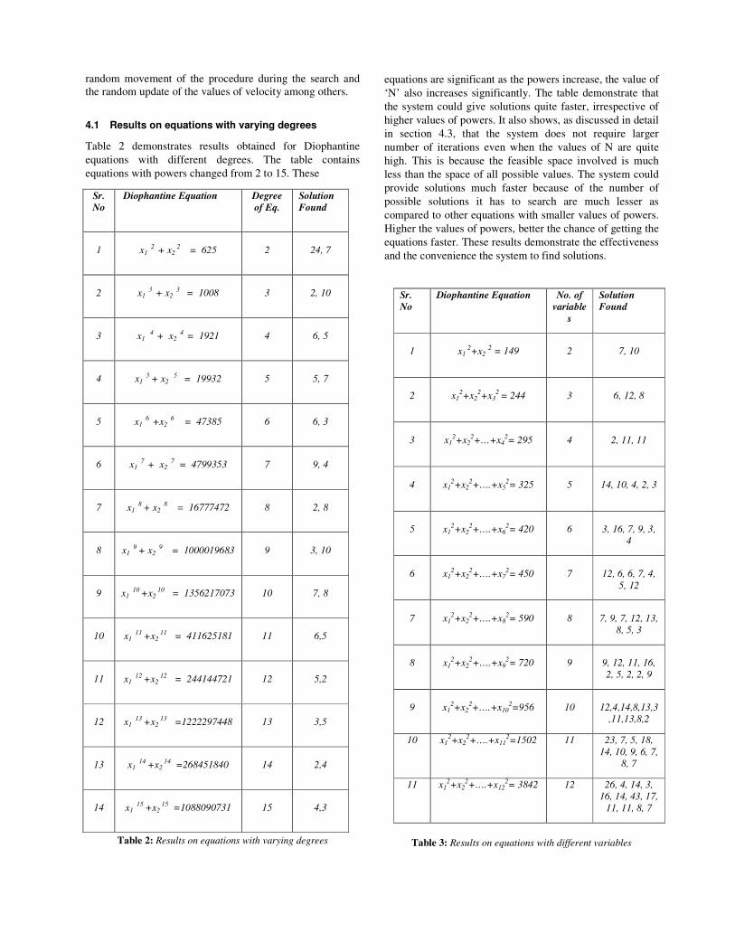
4.1 Results on equations with varying degrees

Table 2 demonstrates results obtained for Diophantine

equations with different degrees. The table contains

equations with powers changed from 2 to 15. These

Table 2: Results on equations with varying degrees

equations are significant as the powers increase, the value of

‘N’ also increases significantly. The table demonstrate that

the system could give solutions quite faster, irrespective of

higher values of powers. It also shows, as discussed in detail

in section 4.3, that the system does not require larger

number of iterations even when the values of N are quite

high. This is because the feasible space involved is much

less than the space of all possible values. The system could

provide solutions much faster because of the number of

possible solutions it has to search are much lesser as

compared to other equations with smaller values of powers.

Higher the values of powers, better the chance of getting the

equations faster. These results demonstrate the effectiveness

and the convenience the system to find solutions.

Table 3: Results on equations with different variables

Sr.

No

Diophantine Equation

Degree

of Eq.

Solution

Found

1

x1 2 + x2

2 = 625

2

24, 7

2

x1 3 + x2

3 = 1008

3

2, 10

3

x1 4 + x2

4 = 1921

4

6, 5

4

x1 5 + x2

5 = 19932

5

5, 7

5

x1 6 +x2

6 = 47385

6

6, 3

6

x1 7 + x2

7 = 4799353

7

9, 4

7

x1 8 + x2

8 = 16777472

8

2, 8

8

x1 9 + x2

9 = 1000019683

9

3, 10

9

x1 10 +x2

10 = 1356217073

10

7, 8

10

x1 11 +x2

11 = 411625181

11

6,5

11

x1 12 +x2

12 = 244144721

12

5,2

12

x1 13 +x2

13 =1222297448

13

3,5

13

x1 14 +x2

14 =268451840

14

2,4

14

x1 15 +x2

15 =1088090731

15

4,3

Sr.

No

Diophantine Equation No. of

variable

s

Solution

Found

1

x1 2+x2

2 = 149

2

7, 10

2

x12+x2

2+x3

2 = 244

3

6, 12, 8

3

x12+x2

2+…+x42= 295

4

2, 11, 11

4

x12+x2

2+….+x52= 325

5

14, 10, 4, 2, 3

5

x12+x2

2+….+x62= 420

6

3, 16, 7, 9, 3,

4

6

x12+x2

2+….+x72= 450

7

12, 6, 6, 7, 4,

5, 12

7

x12+x2

2+….+x82= 590

8

7, 9, 7, 12, 13,

8, 5, 3

8

x12+x2

2+….+x92= 720

9

9, 12, 11, 16,

2, 5, 2, 2, 9

9

x12+x2

2+….+x102=956

10

12,4,14,8,13,3

,11,13,8,2

10 x12+x2

2+….+x112=1502 11 23, 7, 5, 18,

14, 10, 9, 6, 7,

8, 7

11 x12+x2

2+….+x122= 3842 12 26, 4, 14, 3,

16, 14, 43, 17,

11, 11, 8, 7

4.2 Results on equations with varying number of

variables

Table 3 shows the results obtained when the system was run

on Diophantine equations with varying number of variables.

The table consists of a list of equations of representative

nature. Here the equations have the number of variables

change from 2 to 12. As the table shows, the system

provides solutions even when the number of variables is

competitively high. The solutions found show the nature of

solution offered by the procedure. The coordinates of the

solution are varied, different and not closely placed. The

number of generations used to find the solution also reveals

the random nature of the procedure. There is a connection between the number of variables of the equations and the number of generations required to find solutions. If the number of variables is less the system gives the solutions much faster as discussed in the next section.

4.3 Comparing graphs of number of iterations on degree

and no of variables.

Figures 3 and 4 show the relation between generations

required to find solution of a given Diophantine equation

and the type of the equation. Figure 3 conveys the same

between the number of variables in the first nine equations

given in the table 3 and the number of generations used by

the system to find the first solution. It shows that if the

number of variables is less the system provides the solution

much faster. As the number of variables increases the

generations required and hence the time taken to provide a

solution also increases. As the number of variables in an

equation increases, the search space also increases and

hence the complexity of the search becomes large. Hence,

finding of the solution of a given Diophantine equation

becomes a slow process.

Figure 3: No of variables and generation

However, there is no such relation between the number of generations and the powers used in the equations. Figure 4 shows the effect of different of powers in finding the solution of first nine Diophantine equations given in the table 2. The graph shows that there is no apparent connection between the value of the power and the number of generations required. It shows that increase in the maximum power of an equation does not slow down the optimization process. However, in some situations, the procedure could offer the solution much faster than we expected. The powers of an equation do not affect the convergence process because as the powers increase, the search space does not increase substantially on comparison with that of the number of variables. As is the case here, the corresponding increase in values of ‘N’ does not affect the procedure in the faster offering of solution.

Thus, the figure 3 and figure 4 show the slightly

different effect of the number of variables and powers in the

finding of solutions. On comparision, as the number of

variables have much greater say in slowing down the

optimization processs than the powers of an equation. It has

been observed that as the number of variables increase, the

iterations required to find a solution increase tremendously.

This is because,as the number of variables increases, there is

an expoential increase in the number of possible solutions in

the search space.

4.4 Results on equations with varying number of

variables and powers

Table 3 shows the results obtained for different equations

which have both powers and number of variables changed.

These elementary equations are representative in nature and

show the tendency of the system to deal with such the

powers in the range of 2 and 5. The results show the

Figure 4: Powers and generations

similar trend shown by the system in the earlier cases. These

equations have non-identity coefficients unlike the

equations given in table 2 and table 3. The equations have

number of variables change from 3 to 5 and powers do not

have much impact in slowing the system in giving the

solution. However, increasing number of variables has a

deeper impact on the delay in producing the solution. If the

number of variables is large, the system

Table 3: Results on equations with different variables and powers

takes lots of time in giving solution. This is because, as the

number of variables increases, the number of elements in

the search space increases exponentially slowing down the

search substantially.

Figure 5 shows the number of generations required by

these equations to provide the first solutions. Here, the

x- axis represents the serial number of the equations given

in table 3 and y-axis represents the number of generations

required to find the first solution. The figure conveys that

these equations take larger number of iterations to find

solutions on comparing with equations where the powers or

the number of variables alone change. This comparatively

larger number of generations is due to the fact that as both

powers and variables change, there will be large variations

of the fitness values of the particles. This variation is

supported by the non-identity coefficients in the equations.

These coefficients support the fitness value of the concerned

particle change much significantly. Even slight change in

the value of the coordinate has a larger impact on the fitness

value. As the fitness values fluctuate over a larger range, the

process takes time to be steady and mature. When the

procedure becomes stabilized, the procedure is more

directed towards giving solutions.

Figure 5: No of generations

As the variations become more predominant in the initial

stage, the system takes more effort and time to settle the

procedure to direct towards a solution. In this process, as

discussed, the existence of coefficients having values other

one in the equations still reduce the speed of convergence of

the process. This is because larger values of coefficients will

have greater role in the fluctuations of the fitness values and

hence takes more time to settle down. Though, the system

takes little more time to provide the solutions, the figure

suggests that simultaneous influence of variables, powers

and non-identity coefficients can only slightly delay the

process of a finding solution.

4.5 Convergence of pbest Values

Figure 6 shows the convergence of the averages of the

fitness values of the ‘pbest’ particles for the equation

x1 2

+ x2 2

= 4500. Initially, the averages reduce rapidly

and then settle slowly. Finally, the convergence process

gives the solution (60, 30) at the 29th

generation. This is

typical for any convergences procedure of ‘pbest’ averages.

The rapid reduction at the initial stage of the optimization is

due to realization of better ‘pbest’ values initially. Once the

process becomes matured and steady, the ‘pbest’ values

Sr.

No

Diophantine Equation

Solution

Found

1

2x1 2+6 x2

3+ x3 2 = 1825

3,40,6

2

3 x1 3+13 x2 2+10 x3 3= 25632

12,24,36

3

17 x1 3+12 x2 2+2 x3 3= 59050

10,30,25

4

8 x1 4+12 x2

2+2 x3 3+7 x3 3=

97800

10,20,30,40

5

5 x1 5+9 x2

3+3 x3 2+7 x4 2+

2 x52= 60500

5,15,25,35,45

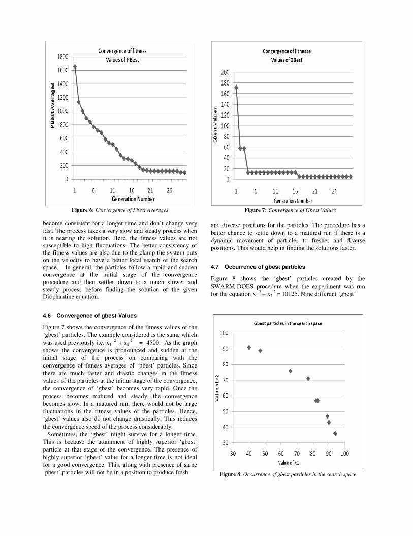
Figure 6: Convergence of Pbest Averages

become consistent for a longer time and don’t change very

fast. The process takes a very slow and steady process when

it is nearing the solution. Here, the fitness values are not

susceptible to high fluctuations. The better consistency of

the fitness values are also due to the clamp the system puts

on the velocity to have a better local search of the search

space. In general, the particles follow a rapid and sudden

convergence at the initial stage of the convergence

procedure and then settles down to a much slower and

steady process before finding the solution of the given

Diophantine equation.

4.6 Convergence of gbest Values

Figure 7 shows the convergence of the fitness values of the

‘gbest’ particles. The example considered is the same which

was used previously i.e. x1 2

+ x2 2

= 4500. As the graph

shows the convergence is pronounced and sudden at the

initial stage of the process on comparing with the

convergence of fitness averages of ‘pbest’ particles. Since

there are much faster and drastic changes in the fitness

values of the particles at the initial stage of the convergence,

the convergence of ‘gbest’ becomes very rapid. Once the

process becomes matured and steady, the convergence

becomes slow. In a matured run, there would not be large

fluctuations in the fitness values of the particles. Hence,

‘gbest’ values also do not change drastically. This reduces

the convergence speed of the process considerably.

Sometimes, the ‘gbest’ might survive for a longer time.

This is because the attainment of highly superior ‘gbest’

particle at that stage of the convergence. The presence of

highly superior ‘gbest’ value for a longer time is not ideal

for a good convergence. This, along with presence of same

‘pbest’ particles will not be in a position to produce fresh

Figure 7: Convergence of Gbest Values

and diverse positions for the particles. The procedure has a

better chance to settle down to a matured run if there is a

dynamic movement of particles to fresher and diverse

positions. This would help in finding the solutions faster.

4.7 Occurrence of gbest particles

Figure 8 shows the ‘gbest’ particles created by the

SWARM-DOES procedure when the experiment was run

for the equation x1 2 + x2

2 = 10125. Nine different ‘gbest’

Figure 8: Occurrence of gbest particles in the search space

positions of the particle where created, which were used in

the subsequent generations to find the positions of the

particles. The graph shows the occurrence of the ‘gbest’

particles in the search of the given Diophantine equation.

The occurrence of these particles are scattered throughout

the search space. The location of such nodes in the search

space demonstrates the directed random nature of the

SWARM-DOES methodology. During the process of

finding numerical solution to the given Diophantine

equation, the procedure could use these ‘gbest’ values

effectively to manoeuvre the search space successfully. The

number of ‘gbest’ particles encountered depends on the type

and nature of the equation. There is no direct relation

between the number of ‘gbest’ particles created and the

solution obtained. The quality of the ‘gbest’ is important

than the number of such particles.

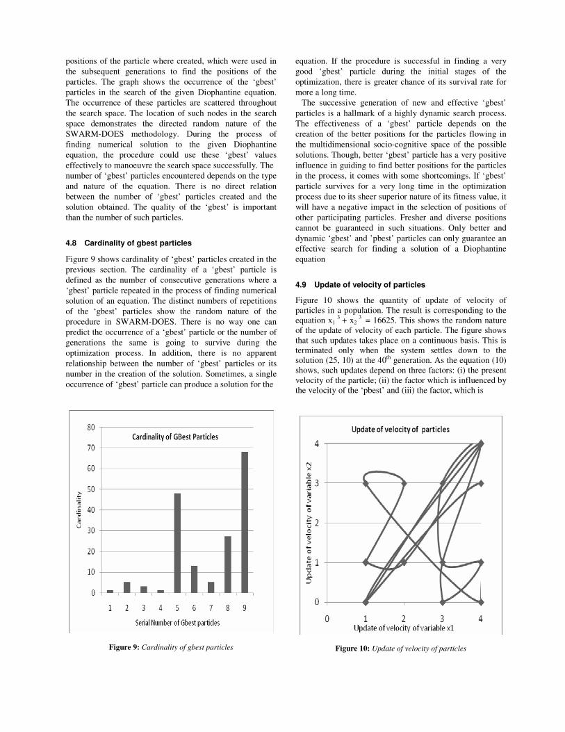
4.8 Cardinality of gbest particles

Figure 9 shows cardinality of ‘gbest’ particles created in the

previous section. The cardinality of a ‘gbest’ particle is

defined as the number of consecutive generations where a

‘gbest’ particle repeated in the process of finding numerical

solution of an equation. The distinct numbers of repetitions

of the ‘gbest’ particles show the random nature of the

procedure in SWARM-DOES. There is no way one can

predict the occurrence of a ‘gbest’ particle or the number of

generations the same is going to survive during the

optimization process. In addition, there is no apparent

relationship between the number of ‘gbest’ particles or its

number in the creation of the solution. Sometimes, a single

occurrence of ‘gbest’ particle can produce a solution for the

Figure 9: Cardinality of gbest particles

equation. If the procedure is successful in finding a very

good ‘gbest’ particle during the initial stages of the

optimization, there is greater chance of its survival rate for

more a long time.

The successive generation of new and effective ‘gbest’

particles is a hallmark of a highly dynamic search process.

The effectiveness of a ‘gbest’ particle depends on the

creation of the better positions for the particles flowing in

the multidimensional socio-cognitive space of the possible

solutions. Though, better ‘gbest’ particle has a very positive

influence in guiding to find better positions for the particles

in the process, it comes with some shortcomings. If ‘gbest’

particle survives for a very long time in the optimization

process due to its sheer superior nature of its fitness value, it

will have a negative impact in the selection of positions of

other participating particles. Fresher and diverse positions

cannot be guaranteed in such situations. Only better and

dynamic ‘gbest’ and ’pbest’ particles can only guarantee an

effective search for finding a solution of a Diophantine

equation

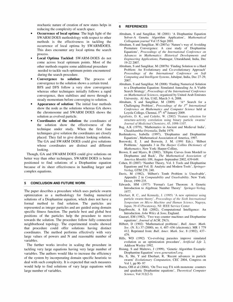
4.9 Update of velocity of particles

Figure 10 shows the quantity of update of velocity of

particles in a population. The result is corresponding to the

equation x1 3

+ x2 3

= 16625. This shows the random nature

of the update of velocity of each particle. The figure shows

that such updates takes place on a continuous basis. This is

terminated only when the system settles down to the

solution (25, 10) at the 40th

generation. As the equation (10)

shows, such updates depend on three factors: (i) the present

velocity of the particle; (ii) the factor which is influenced by

the velocity of the ‘pbest’ and (iii) the factor, which is

Figure 10: Update of velocity of particles

influenced by the velocity of ‘gbest’ of the particle. The

updates within a smaller range of (0, 4) is due to the

restriction the system imposed on the velocity changes,

which was facilitated using vmax. The presence of vmax

restricts the update of larger values and hence the large

variation in the positions of the particles. Such a clamp on

velocity provides better and thorough local search in the

process of finding numerical solution of a Diophantine

equation. If the vmax was not available, the velocity values

would have taken larger updates and hence particle might

take positions, by skipping the solution position in the

process.

4.10 Statistical measures of Fitness function

Figure 11 shows different statistical measures generated

corresponding to the equation x12

+ x22

= 10000. The

statistical measures used are mean, median and standard

deviation. The measures are based on the fitness values of

the particles in the SWARM-DOES process. These

Figure 11: Measures of values of fitness function

measures reveal the characteristics of the optimization

process undertaken in the procedure. The graph shows that

mean and median show a random and fluctuating nature of

the fitness function values encountered in the procedure.

Initially, there is much deeper change in these measures due

to better positions encountered by particles. Once the

process becomes stabilized and mature, such drastic changes

become less. Both the measures mean and median show

similar tendency as the figure shows. It reveals that the

process has a stabilization capacity inbuilt in the procedure.

The standard deviation lies within a small range showing

the effectiveness of the procedure to direct towards the

solution even when randomness plays its role. It shows the

lesser variability of the fitness values of the particles with

respect to its mean value during the process of finding

solution to a Diophantine equation. These measures as a

whole demonstrate the inbuilt strength and capacity to steer

the complex search space quite effectively.

4.11 Effect of population size

Figure 12 shows the effect of population size on speeding

up the optimization process. The figure shows the results

obtained for the equation x12

+ x22

= 2600. The experiments

were conducted for the equation with different population

size as mentioned. The number of particles taken in the

experiment varied from 10 to 100 with an interval of 10. If

the population size is very small, the number of generation

required for finding a solution is comparatively large. Any

population size in the vicinity of around 30 to 50 is

sufficiently good. After that, just by increasing the

population size does not give much better result. Though the

results were shown for an elementary equation, similar

results were obtained for other equations also.

Figure 12: Effect of population size

4.12 Comparison with other techniques

Table 5 gives the comparative study of the results obtained

by SWARM DOES methodology with other techniques.

The techniques covered in the discussion are BFS, DFS,

Steepest Ascent Hill Climbing, A* Algorithm, Genetic

algorithm and SWARM DOES. The comparative study has

been done on parameters which are common to the

techniques discussed.

• Representation of solutions: The candidate

solutions are represented as vectors in all methods

except on GA and SWARM DOES where they are

represented as chromosomes (or strings) and

particles respectively. The proper representation

helps to find solution of the equation in each of the

case. The vector representation comes quite natural

to the first four methods as the same is in sync with

the requirement of these algorithms. The string

representation in GA helps to have the meeting of

the proper requirements of the particular equation

along with that of the genetic algorithm. The

particles in the SWARM DOES system are

represented as arrays.

• Computation Style: The computation style

followed in the methods is sequential except on

GA and SWARM-DOES where the style is

parallel. The parallel computation style of the GA

and SWARM-DOES works effectively while

dealing with huge number of candidate solutions in

the search space. In the case of GA, a population of

strings are in search of solutions concurrently

while in the case of SWARM DOES, a population

of swarm perform at the search. This parallel

computing framework of chromosomes or particles

help to find the solutions of the equation much

more effectively than other algorithms discussed in

the work.

• Procedure type: The procedure followed in all the

techniques except GA and SWARM DOES are

deterministic where they follow randomly.

Though, the sequential way of moving towards the

solution have many advantages, especially when

the equations are elementary and easy to manage,

often they bring lot of computational complexity.

These methods are not guaranteed to give solutions

when the equations are quite large and the value of

‘N’ is very high as the number of candidate

solutions in the search space is extremely large.

The directed random nature of GA and SWARM-

DOES are effective in managing the complexity of

search space.

• Mathematical structure: The mathematical

structure followed in BFS, DFS, A* and Hill

Climbing are tree structure. Nodes are generated as

and when a new candidate state is searched and

finding solution is translated to traversing through

the tree. While GA does not have a formal

mathematical structure, SWARM DOES follows

a proper structure. It uses fully connected graph as

the neighbourhood topology. Through this, the

procedure maintains a relation between each and

every particles participating in the optimization

process. It helps to keep track of each particle and

link with its best performance, which is

incorporated in the procedure for optimum results.

The linking with the all the particles in the

population, not just a couple of neighbours, help to

fine tune each particle’s search mechanism in a

way that is in tune with the best performance of

other particles.

• New states formed: The new candidate solutions

are formed using typical production rules in the

first four techniques where as GA and

SWARMDOES follow stochastically. The

Table 5: Comparative study

Character

istics.

BFS

DFS

A*

Hill

Climbi

ng

GA

SWAR

M

DOES

Represe

ntation of

solution

Vecto

r

Vecto

r

Vector

Vecto

r

Chro

moso

mes

Partic

les

Computational

style

Seque

ntial

Seque

ntial

Seque

ntial

Seque

ntial

Parall

el

Parall

el

Procedu

re type

Deter-

minist

ic

Deter

minist

ic

Deter

minist

ic

Deter

minist

ic

Rand

om

Rand

om

Mathe-

matical

struct-

ure

Tree

Tree

Tree

Tree

NA

Grap

h

New

state

formed

Using

produ

ct-ion

rules

Using

produ

ct-ion

rules

Using

produ

ct-ion

rules

Using

produ

ct-ion

rules

Stoch

a-

sticall

y

Stoch

a-

sticall

y

Occurre

nce of Local

Optima

No

Yes

No

Yes

Yes

No

Local

optima

Tackled

NA

Back

tracki

ng

NA

Back

tracki

ng

By

Coevo

lution

NA

Converg

ence to

solution

Slow

Slow

Rapid,

then

steady

Rapid

, then

steady

Rapid

, then

steady

Rapid

, then

steady

Appear-

ance of

Solution

Node

Node

Node

Node

Evolv

ed-

chrom

Evolv

ed-

partic

le

Coordin

ates of

solution

Close

Close

Close

Close

Distin

ct

Distin

ct

stochastic nature of creation of new states helps in

reducing the complexity of search space.

• Occurrence of local optima: The high light of the

SWARM DOES methodology with respect to other

methods is the effectiveness in tackling the

occurrence of local optima by SWARMDOES.

This does encounter any local optima the search

process.

• Local Optima Tackled: SWARM-DOES do not

come across local optimum points. Most of the

other methods require some additional procedure

needed to tackle such optimum points encountered

during the search procedure.

• Convergence to solution: The process of

convergence to the solution shows a certain trend.

BFS and DFS follow a very slow convergence

whereas other techniques initially follows a rapid

convergence, then stabilises and move through a

steady momentum before converging to solution.

• Appearance of solution: The initial four methods

show the node as the solutions whereas GA shows

the chromosome and SWARM DOES shows the

solution as evolved particle.

• Coordinates of the solution: the coordinates of

the solution show the effectiveness of the

technique under study. When the first four

techniques give solution the coordinates are closely

placed. They fail to give distinct looking solution.

The GA and SWARM DOES could give solutions

whose coordinates are distinct and different

looking.

Though, GA and SWARM DOES could give solutions on

better way than other techniques, SWARM DOES is better

positioned to find solutions of a Diophantine equation

because of its sheer effectiveness in handling larger and

complex equations.

5 CONCLUSION AND FUTURE WORK

The paper describes a procedure which uses particle swarm

optimization as a methodology for finding numerical

solutions of a Diophantine equation, which does not have a

formal method to find solution. The particles are

represented as integer particles and are guided using domain

specific fitness function. The particle best and global best

positions of the particles help the procedure to move

towards the solution. The procedure follow fully connected

neighborhood topology. The experimental results showed

that procedure could offer solutions having distinct

coordinates. The method performs effectively with very

large values of powers and N and reasonable number of

variables.

The further works involve in scaling the procedure in

tackling very large equations having very large number of

variables. The authors would like to increase the efficiency

of the system by incorporating domain specific heuristic to

deal with such complexity. It is expected that such measures

would help to find solutions of vary large equations with

large number of variables.

6 REFERENCES

Abraham, S and Sanglikar, M (2001) ‘A Diophantine Equation Solver-A Genetic Algorithm Application’, Mathematical

Colloquium journal Vol 15 Sept 2001. Abraham, S and Sanglikar, M (2007a) ‘Nature’s way of Avoiding

Premature Convergence: A case study of Diophantine Equations’, Proceedings of the International Conference on Advances in Mathematics: Historical Developments and Engineering Applications, Pantnagar, Uttarakhand, India, Dec 19-22 2007.

Abraham, S and Sanglikar, M (2007b) ‘Finding Solution to a Hard Problem: An Evolutionary and Co-evolutionary Approach’ Proceedings of the International Conference on Soft Computing and Intelligent Systems, Jabalpur, India, Dec 27-29, 2007.

Abraham, S and Sanglikar, M (2008) ‘Finding Numerical Solution to a Diophantine Equation: Simulated Annealing As A Viable Search Strategy’, Proceedings of the International Conference

on Mathematical Sciences, organized by United Arab Emirates University, Al Ain, UAE, March 3- 6, 2008.

Abraham, S and Sanglikar, M (2009) ‘A* Search for a Challenging Problem’, Proceedings of the 3rd International Conference on Mathematics and Computer Science held at Loyola College, Chennai, 5th- 6th January 2009.

Agrafiotis, D. K., and Cedeño, W. (2002) ‘Feature selection for structure-activity correlation using binary particle swarms’ Journal of Medicinal Chemistry, 45, 1098-1107.

Bag, A.K (1979), ‘Mathematics in Ancient and Medieval India’, Chaukhambha Orientalia, Delhi 1979.

Bashmakova, Isabella (1997), ‘Diophantus and Diophantine Equations’, Mathematical Association of America, 1997.

Borowski, E. J. and Borwein, J. M. (1991 Eds.). ‘Hilbert Problems.’ Appendix 3 in The Harper Collins Dictionary of

Mathematics, New York: Harper-Collins, Brown, E and Myers, B (2002), ‘Elliptic Curves from Mordell to

Diophantus and Back’, The Mathematical Association of

America Monthly 109, August–September 2002, 639-649. Cohen, H (2007) ‘Number Theory, Vol. I: Tools and Diophantine

Equations and Vol. II: Analytic and Modern Tools’, Springer-

Verlag, GTM 239, 240. Davis, M (1982), ‘Hilbert's Tenth Problem is Unsolvable’,

Appendix 2 in Computability and Unsolvability. New York: Dover, 1999-235.

Edwards, HM (1977) ‘Fermat's Last Theorem: A Genetic Introduction to Algebraic Number Theory’ Springer-Verlag. 1977.

Eberhart, R. C., and Kennedy, J. (1995) ‘A new optimizer using particle swarm theory’, Proceedings of the Sixth International

Symposium on Micro Machine and Human Science, Nagoya, Japan, 39-43.Piscataway, NJ: IEEE Service Center

Engelbrecht, A Edi (2002), Computational Intelligence: An Introduction. John Wiley & Sons, England.

Guarari, EM (1982), ‘Two way counter machines and Diophantine equations’, Journal of ACM, 29(3).

Hilbert, D (1902) ‘Mathematical problems’, Bull. Amer. Math. Soc. (N. S.) 37 (2000), no. 4, 407–436 (electronic). MR 1 779 412. Reprinted from: Bull. Amer. Math. Soc. 8 (1902), 437–479.

Hills, WD (1992) ‘Co-evolving parasites improve simulated evolution as an optimization procedure’, Artificial Life 2, Addison Wesley 1992.

Hsiung, S and Mattews, J (1999), ‘Genetic Algorithm Example: Diophantine Equation’ www.generation5.org.

Hu, X, Shi, Y and Eberhart, R, ‘Recent advances in particle swarm’ Evolutionary Computation, CEC 2004, Congress on Vol 1, pp 90- 97

Ibarra, OH et al (2004), ‘On Two way FA with monotone counters and quadratic Diophantine equations’, Theoretical Computer Science, Vol 312(2-3)

Joya, G, Atencla, M. A. and Sandoval, F., ‘Application of Higher order Hopfield neural networks to the solution of Diophantine equation’, Lecture Notes in Computer Science, Springer Berlin / Heidelberg, Volume 540/1991

Kennedy, J and Eberhart, R (1995), ‘Particle swarm optimization’ Proc. of the IEEE Int. Conf. on Neural Networks, Piscataway, NJ, pp. 1942–1948.

Kennedy, J and Eberhart, R (1997), ‘A discrete binary version of the particle swarm algorithm’. Proc. of Conf. on Systems, Man, and Cybernetics, 4104-4109. Piscataway, NJ: IEEE Service Center.

Kennedy, J (1999). ‘Small worlds and mega minds: Effects of neighborhood topology on particle swarm performance’ Proceeding of the 1999 Conference on Evolutionary Computation, 1931-1938.

Kennedy J., and Mendes, R. (2002) ‘Population structure and particle swarm performance’, Proceeding of the 2002 Congress on Evolutionary Computation, Honolulu, Hawaii, May 12-17,

Koblitz, Neil (1984) ‘Introduction to Elliptic Curves and Modular Forms’ Springer- Verlag.

Laih CS et al (1997), ‘Cryptanalysis of Diophantine equation oriented public key cryptosystem’, IEEE Transactions on Computers, Vol 46, April 1997.

Lin, CH et al (1995): Lin CH et al: ‘A new public-key cipher system based upon Diophantine equations’, IEEE Transactions on Computers, Vol 44, Jan 1995.

Luger (2006): George Lugar, “Artificial Intelligence: Structures and Strategies for Complex Problem solving”, 4e Pearson Education.

Matiyasevich, YV (1993), ‘Hilbert’s Tenth Problem’, MIT press

1993. Michalewich (1992) ‘GA + Data Structures = Evaluation

Programs’, Springer Verlag 1992

Paredis, J (1996), ‘Coevolutionary Computation’, Artificial Life Journal, 2(3), 1996.

Poonen, B(2000), ‘Computing Rational Points On Curves’, Proceedings of the Millennial Conference on Number Theory, University of Illinois at Urbana-Champaign, May 21–26.

Ratnaweera, A., Halgamuge, S. K., and Watson, H. C. (2004). ‘Self-organizing hierarchical particle swarm optimizer with time varying accelerating Coefficients’. IEEE Transactions on Evolutionary Computation

Rosin and Belew (1997) ‘New methods for competitive coevolution’ Evolutionary Computation 5(1):1–29.

Rossen, Kenneth (1987), ‘Elementary Number theory and its applications’, Addison-Wesley Publication.

Russell and Norwig (2003), ‘Artificial Intelligence-A modern approach’ Second Edition, Pearson Publication

Shi, Y and Eberhart R. C(1998), ‘A modified particle swarm optimizer’, Proceedings of the IEEE Congress on Evolutionary Computation, Piscatway, NJ, pp.69-73.

Shi, Y., and Eberhart, R. C. (1998a), ‘Parameter selection in particle swarm optimization’ Proceedings of the 1998 Annual Conference on Evolutionary Computation, March 1998

Shi, Y., and Eberhart, R. C. (1999), ‘Empirical study of particle swarm optimization’ Proceedings of the 1999 Congress on Evolutionary Computation, 1945-1950.Piscataway, NJ: IEEE Service Center.

Shi, Y., and Eberhart, R. C. (2001a). Fuzzy adaptive particle swarm optimization, Proc.Congress on Evolutionary Computation 2001, Seoul, Korea. Piscataway, NJ: IEEE Service Center.

Shi, Y., and Eberhart, R. C. (2001b), ‘Particle swarm optimization with fuzzy adaptive inertia weight’, Proceedings of the Workshop on Particle Swarm Optimization 2001, Indianapolis, IN.

Shi, Y (2004), ‘Particle Swarm Optimization’, IEEE Neural Network Society, February 2004

Shirali, S and Yogananda, CS (2003), ‘Fermat’s Last Theorem: A Theorem at Last’, Number theory: Echoes from resonance, University press.

Sierra, M and Coello, C (2006), ‘Multiobjective particle swarm optimizers: A survey if the state of the art’, International journal of computational intelligence and research Vol.2, No.3 (2006), pp. 287–308

Stroeker and Tzanakis (1994), ‘Solving elliptic Diophantine equations by estimating linear forms in elliptic logarithms’, Acta Arithmetica LXVII.2.

Tzen, TH and Ni LM (1993), ‘Trapezoid self-scheduling: a practical scheduling scheme for parallel compilers’, IEEE Trans. Parallel Distributed Systems, 4(1), 87-98.

Velu (2000]: Velu, Pillai K, ‘Computable Economics: The Arne Memorial Lecture Series’, Oxford University Press, 2000

Wiegand, P (2003) ‘An Analysis of Cooperative Coevolutionary Algorithms’, PhD dissertation, George Mason University 2003.

Zhiyu, S, Li Z, Yew, PC (1989), ‘An Empirical study on array subscripts and data dependencies’, CSRD Report 840, August

Zuckerman, N (1980), ‘An introduction to the theory of numbers’, 3rd edition, Wiley Publication, 1980

WEBSITES

http://www.swarmintelligence.org http://www.softcomputing.net http://www.mauriceclerc.net. http://www.wikipedia.org http://www.scholarpedia.org http://www.birs.ca/workshops/2007/07w5063/report07w5063

(