particle swarm optimization -...

Chapter 16

Particle Swarm Optimization

The particle swarm optimization (PSO) algorithm is a population-based search al-gorithm based on the simulation of the social behavior of birds within a flock. Theinitial intent of the particle swarm concept was to graphically simulate the gracefuland unpredictable choreography of a bird flock [449], with the aim of discovering pat-terns that govern the ability of birds to fly synchronously, and to suddenly changedirection with a regrouping in an optimal formation. From this initial objective, theconcept evolved into a simple and efficient optimization algorithm.

In PSO, individuals, referred to as particles, are “flown” through hyperdimensionalsearch space. Changes to the position of particles within the search space are basedon the social-psychological tendency of individuals to emulate the success of otherindividuals. The changes to a particle within the swarm are therefore influenced bythe experience, or knowledge, of its neighbors. The search behavior of a particle isthus affected by that of other particles within the swarm (PSO is therefore a kind ofsymbiotic cooperative algorithm). The consequence of modeling this social behavioris that the search process is such that particles stochastically return toward previouslysuccessful regions in the search space.

The remainder of this chapter is organized as follows: An overview of the basic PSO,i.e. the first implementations of PSO, is given in Section 16.1. The very importantconcepts of social interaction and social networks are discussed in Section 16.2. Basicvariations of the PSO are described in Section 16.3, while more elaborate improvementsare given in Section 16.5. A discussion of PSO parameters is given in Section 16.4.Some advanced topics are discussed in Section 16.6.

16.1 Basic Particle Swarm Optimization

Individuals in a particle swarm follow a very simple behavior: to emulate the success ofneighboring individuals and their own successes. The collective behavior that emergesfrom this simple behavior is that of discovering optimal regions of a high dimensionalsearch space.

A PSO algorithm maintains a swarm of particles, where each particle represents apotential solution. In analogy with evolutionary computation paradigms, a swarm is

Computational Intelligence: An Introduction, Second Edition A.P. Engelbrechtc©2007 John Wiley & Sons, Ltd

289

290 16. Particle Swarm Optimization

similar to a population, while a particle is similar to an individual. In simple terms,the particles are “flown” through a multidimensional search space, where the positionof each particle is adjusted according to its own experience and that of its neighbors.Let xi(t) denote the position of particle i in the search space at time step t; unlessotherwise stated, t denotes discrete time steps. The position of the particle is changedby adding a velocity, vi(t), to the current position, i.e.

xi(t + 1) = xi(t) + vi(t + 1) (16.1)

with xi(0) ∼ U(xmin,xmax).

It is the velocity vector that drives the optimization process, and reflects both theexperiential knowledge of the particle and socially exchanged information from theparticle’s neighborhood. The experiential knowledge of a particle is generally referredto as the cognitive component, which is proportional to the distance of the particlefrom its own best position (referred to as the particle’s personal best position) foundsince the first time step. The socially exchanged information is referred to as the socialcomponent of the velocity equation.

Originally, two PSO algorithms have been developed which differ in the size of theirneighborhoods. These two algorithms, namely the gbest and lbest PSO, are summa-rized in Sections 16.1.1 and 16.1.2 respectively. A comparison between gbest and lbestPSO is given in Section 16.1.3. Velocity components are decsribed in Section 16.1.4,while an illustration of the effect of velocity updates is given in Section 16.1.5. Aspectsabout the implementation of a PSO algorithm are discussed in Section 16.1.6.

16.1.1 Global Best PSO

For the global best PSO, or gbest PSO, the neighborhood for each particle is the entireswarm. The social network employed by the gbest PSO reflects the star topology(refer to Section 16.2). For the star neighborhood topology, the social component ofthe particle velocity update reflects information obtained from all the particles in theswarm. In this case, the social information is the best position found by the swarm,referred to as y(t).

For gbest PSO, the velocity of particle i is calculated as

vij(t + 1) = vij(t) + c1r1j(t)[yij(t)− xij(t)] + c2r2j(t)[yj(t)− xij(t)] (16.2)

where vij(t) is the velocity of particle i in dimension j = 1, . . . , nx at time stept, xij(t) is the position of particle i in dimension j at time step t, c1 and c2 arepositive acceleration constants used to scale the contribution of the cognitive andsocial components respectively (discussed in Section 16.4), and r1j(t), r2j(t) ∼ U(0, 1)are random values in the range [0, 1], sampled from a uniform distribution. Theserandom values introduce a stochastic element to the algorithm.

The personal best position, yi, associated with particle i is the best position theparticle has visited since the first time step. Considering minimization problems, the

16.1 Basic Particle Swarm Optimization 291

personal best position at the next time step, t + 1, is calculated as

yi(t + 1) ={

yi(t) if f(xi(t + 1)) ≥ f(yi(t))xi(t + 1) if f(xi(t + 1)) < f(yi(t))

(16.3)

where f : Rnx → R is the fitness function. As with EAs, the fitness function measureshow close the corresponding solution is to the optimum, i.e. the fitness functionquantifies the performance, or quality, of a particle (or solution).

The global best position, y(t), at time step t, is defined as

y(t) ∈ {y0(t), . . . ,yns(t)}|f(y(t)) = min{f(y0(t)), . . . , f(yns

(t))} (16.4)

where ns is the total number of particles in the swarm. It is important to note thatthe definition in equation (16.4) states that y is the best position discovered by anyof the particles so far – it is usually calculated as the best personal best position. Theglobal best position can also be selected from the particles of the current swarm, inwhich case [359]

y(t) = min{f(x0(t)), . . . , f(xns(t))} (16.5)

The gbest PSO is summarized in Algorithm 16.1.

Algorithm 16.1 gbest PSO

Create and initialize an nx-dimensional swarm;repeat

for each particle i = 1, . . . , ns do//set the personal best positionif f(xi) < f(yi) then

yi = xi;end//set the global best position if f(yi) < f(y) then

y = yi;end

endfor each particle i = 1, . . . , ns do

update the velocity using equation (16.2);update the position using equation (16.1);

enduntil stopping condition is true;

16.1.2 Local Best PSO

The local best PSO, or lbest PSO, uses a ring social network topology (refer to Sec-tion 16.2) where smaller neighborhoods are defined for each particle. The social compo-nent reflects information exchanged within the neighborhood of the particle, reflectinglocal knowledge of the environment. With reference to the velocity equation, the social


contribution to particle velocity is proportional to the distance between a particle andthe best position found by the neighborhood of particles. The velocity is calculated as

vij(t + 1) = vij(t) + c1r1j(t)[yij(t)− xij(t)] + c2r2j(t)[yij(t)− xij(t)] (16.6)

where yij is the best position, found by the neighborhood of particle i in dimension j.The local best particle position, yi, i.e. the best position found in the neighborhoodNi, is defined as

yi(t + 1) ∈ {Ni|f(yi(t + 1)) = min{f(x)}, ∀x ∈ Ni} (16.7)

with the neighborhood defined as

Ni = {yi−nNi(t),yi−nNi

+1(t), . . . ,yi−1(t),yi(t),yi+1(t), . . . ,yi+nNi(t)} (16.8)

for neighborhoods of size nNi. The local best position will also be referred to as the

neighborhood best position.

It is important to note that for the basic PSO, particles within a neighborhood haveno relationship to each other. Selection of neighborhoods is done based on particleindices. However, strategies have been developed where neighborhoods are formedbased on spatial similarity (refer to Section 16.2).

There are mainly two reasons why neighborhoods based on particle indices are pre-ferred:

1. It is computationally inexpensive, since spatial ordering of particles is not re-quired. For approaches where the distance between particles is used to formneighborhoods, it is necessary to calculate the Euclidean distance between allpairs of particles, which is of O(n2

s) complexity.

2. It helps to promote the spread of information regarding good solutions to allparticles, irrespective of their current location in the search space.

It should also be noted that neighborhoods overlap. A particle takes part as a memberof a number of neighborhoods. This interconnection of neighborhoods also facilitatesthe sharing of information among neighborhoods, and ensures that the swarm con-verges on a single point, namely the global best particle. The gbest PSO is a specialcase of the lbest PSO with nNi

= ns.

Algorithm 16.2 summarizes the lbest PSO.

16.1.3 gbest versus lbest PSO

The two versions of PSO discussed above are similar in the sense that the social com-ponent of the velocity updates causes both to move towards the global best particle.This is possible for the lbest PSO due to the overlapping neighborhoods.

There are two main differences between the two approaches with respect to theirconvergence characteristics [229, 489]:


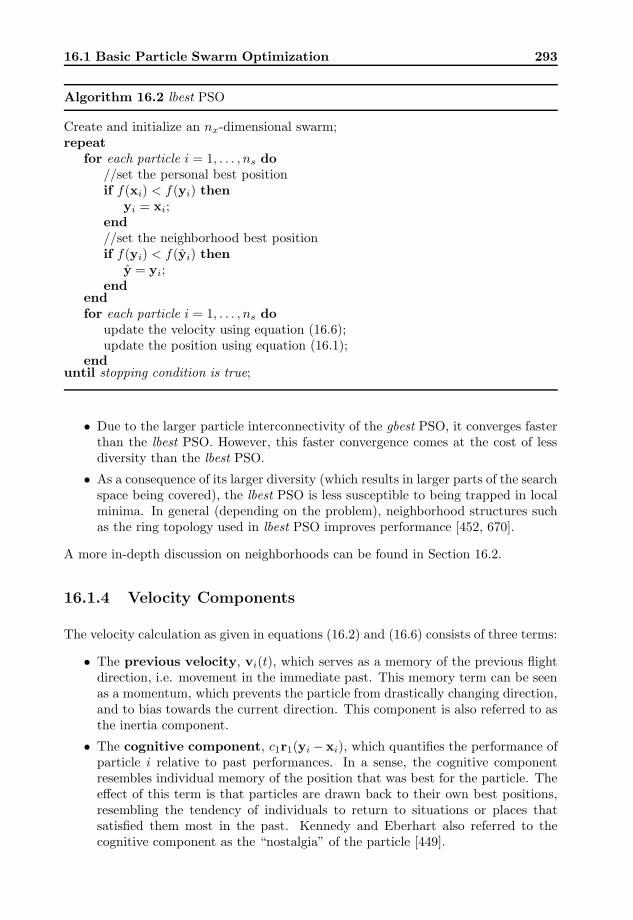
Algorithm 16.2 lbest PSO


for each particle i = 1, . . . , ns do//set the personal best positionif f(xi) < f(yi) then

yi = xi;end//set the neighborhood best positionif f(yi) < f(yi) then

y = yi;end




• Due to the larger particle interconnectivity of the gbest PSO, it converges fasterthan the lbest PSO. However, this faster convergence comes at the cost of lessdiversity than the lbest PSO.

• As a consequence of its larger diversity (which results in larger parts of the searchspace being covered), the lbest PSO is less susceptible to being trapped in localminima. In general (depending on the problem), neighborhood structures suchas the ring topology used in lbest PSO improves performance [452, 670].

A more in-depth discussion on neighborhoods can be found in Section 16.2.

16.1.4 Velocity Components

The velocity calculation as given in equations (16.2) and (16.6) consists of three terms:

• The previous velocity, vi(t), which serves as a memory of the previous flightdirection, i.e. movement in the immediate past. This memory term can be seenas a momentum, which prevents the particle from drastically changing direction,and to bias towards the current direction. This component is also referred to asthe inertia component.

• The cognitive component, c1r1(yi − xi), which quantifies the performance ofparticle i relative to past performances. In a sense, the cognitive componentresembles individual memory of the position that was best for the particle. Theeffect of this term is that particles are drawn back to their own best positions,resembling the tendency of individuals to return to situations or places thatsatisfied them most in the past. Kennedy and Eberhart also referred to thecognitive component as the “nostalgia” of the particle [449].


social velocity

cognitive velocity

inertia velocity

new velocity

x(t)y(t)

x(t + 1)

y(t)

x1

x2

(a) Time Step t

new velocity

cognitive velocity

social velocity

inertiavelocity

x(t)

y(t + 1)

x1

x2

y(t + 1)

x(t + 1)

x(t + 2)

(b) Time Step t + 1

Figure 16.1 Geometrical Illustration of Velocity and Position Updates for a SingleTwo-Dimensional Particle

• The social component, c2r2(y−xi), in the case of the gbest PSO or, c2r2(yi−xi), in the case of the lbest PSO, which quantifies the performance of particle irelative to a group of particles, or neighbors. Conceptually, the social componentresembles a group norm or standard that individuals seek to attain. The effect ofthe social component is that each particle is also drawn towards the best positionfound by the particle’s neighborhood.

The contribution of the cognitive and social components are weighed by a stochasticamount, c1r1 or c2r2, respectively. The effects of these weights are discussed in moredetail in Section 16.4.

16.1.5 Geometric Illustration

The effect of the velocity equation can easily be illustrated in a two-dimensional vectorspace. For the sake of the illustration, consider a single particle in a two-dimensionalsearch space.

An example movement of the particle is illustrated in Figure 16.1, where the particlesubscript has been dropped for notational convenience. Figure 16.1(a) illustrates thestate of the swarm at time step t. Note how the new position, x(t + 1), moves closertowards the global best y(t). For time step t + 1, as illustrated in Figure 16.1(b),assume that the personal best position does not change. The figure shows how thethree components contribute to still move the particle towards the global best particle.

It is of course possible for a particle to overshoot the global best position, mainly dueto the momentum term. This results in two scenarios:

1. The new position, as a result of overshooting the current global best, may be a


better position than the current global best. In this case the new particle positionwill become the new global best position, and all particles will be drawn towardsit.

2. The new position is still worse than the current global best particle. In subse-quent time steps the cognitive and social components will cause the particle tochange direction back towards the global best.

The cumulative effect of all the position updates of a particle is that each particleconverges to a point on the line that connects the global best position and the personalbest position of the particle. A formal proof can be found in [863, 870].

x2

x1

y

(a) At time t = 0

x2

x1

y

(b) At time t = 1

Figure 16.2 Multi-particle gbest PSO Illustration

Returning to more than one particle, Figure 16.2 visualizes the position updates withreference to the task of minimizing a two-dimensional function with variables x1 andx2 using gbest PSO. The optimum is at the origin, indicated by the symbol ‘×’.Figure 16.2(a) illustrates the initial positions of eight particles, with the global bestposition as indicated. Since the contribution of the cognitive component is zero for eachparticle at time step t = 0, only the social component has an influence on the positionadjustments. Note that the global best position does not change (it is assumed thatvi(0) = 0, for all particles). Figure 16.2(b) shows the new positions of all the particlesafter the first iteration. A new global best position has been found. Figure 16.2(b) nowindicates the influence of all the velocity components, with particles moving towardsthe new global best position.

Finally, the lbest PSO, as illustrated in Figure 16.3, shows how particles are influencedby their immediate neighbors. To keep the graph readable, only some of the movementsare illustrated, and only the aggregate velocity direction is indicated. In neighborhood1, both particles a and b move towards particle c, which is the best solution withinthat neighborhood. Considering neighborhood 2, particle d moves towards f , so doese. For the next iteration, e will be the best solution for neighborhood 2. Now d and


x

x 1

2

i

g ba

c

h

efk

j

1

2

3

4

d

(a) Local Best Illustrated – Initial Swarm

x

x 1

2

f d

e

2

(b) Local Best – Second Swarm

Figure 16.3 Illustration of lbest PSO

f move towards e as illustrated in Figure 16.3(b) (only part of the solution space isillustrated). The blocks represent the previous positions. Note that e remains the bestsolution for neighborhood 2. Also note the general movement towards the minimum.

More in-depth analyses of particle trajectories can be found in [136, 851, 863, 870].

16.1.6 Algorithm Aspects

A few aspects of Algorithms 16.1 and 16.2 still need to be discussed. These aspectsinclude particle initialization, stopping conditions and defining the terms iteration andfunction evaluation.

With reference to Algorithms 16.1 and 16.2, the optimization process is iterative. Re-peated iterations of the algorithms are executed until a stopping condition is satisfied.One such iteration consists of application of all the steps within the repeat...untilloop, i.e. determining the personal best positions and the global best position, andadjusting the velocity of each particle. Within each iteration, a number of functionevaluations (FEs) are performed. A function evaluation (FE) refers to one calculationof the fitness function, which characterizes the optimization problem. For the basicPSO, a total of ns function evaluations are performed per iteration, where ns is thetotal number of particles in the swarm.

The first step of the PSO algorithm is to initialize the swarm and control parameters.In the context of the basic PSO, the acceleration constants, c1 and c2, the initial veloc-ities, particle positions and personal best positions need to be specified. In addition,the lbest PSO requires the size of neighborhoods to be specified. The importance ofoptimal values for the acceleration constants are discussed in Section 16.4.


Usually, the positions of particles are initialized to uniformly cover the search space. Itis important to note that the efficiency of the PSO is influenced by the initial diversityof the swarm, i.e. how much of the search space is covered, and how well particles aredistributed over the search space. If regions of the search space are not covered by theinitial swarm, the PSO will have difficulty in finding the optimum if it is located withinan uncovered region. The PSO will discover such an optimum only if the momentumof a particle carries the particle into the uncovered area, provided that the particleends up on either a new personal best for itself, or a position that becomes the newglobal best.

Assume that an optimum needs to be located within the domain defined by the twovectors, xmin and xmax, which respectively represents the minimum and maximumranges in each dimension. Then, an efficient initialization method for the particlepositions is:

x(0) = xmin,j + rj(xmax,j − xmin,j), ∀j = 1, . . . , nx, ∀i = 1, . . . , ns (16.9)

where rj ∼ U(0, 1).

The initial velocities can be initialized to zero, i.e.

vi(0) = 0 (16.10)

While it is possible to also initialize the velocities to random values, it is not necessary,and it must be done with care. In fact, considering physical objects in their initialpositions, their velocities are zero – they are stationary. If particles are initialized withnonzero velocities, this physical analogy is violated. Random initialization of positionvectors already ensures random positions and moving directions. If, however, velocitiesare also randomly initialized, such velocities should not be too large. Large initialvelocities will have large initial momentum, and consequently large initial positionupdates. Such large initial position updates may cause particles to leave the boundariesof the search space, and may cause the swarm to take more iterations before particlessettle on a single solution.

The personal best position for each particle is initialized to the particle’s position attime step t = 0, i.e.

yi(0) = xi(0) (16.11)

Different initialization schemes have been used by researchers to initialize the particlepositions to ensure that the search space is uniformly covered: Sobol sequences [661],Faure sequences [88, 89, 90], and nonlinear simplex method [662].

While it is important for application of the PSO to solve real-world problems, in thatparticles are uniformly distributed over the entire search space, uniformly distributedparticles are not necessarily good for empirical studies of different algorithms. Thistypical initialization method can give false impressions of the relative performance ofalgorithms as shown in [312]. For many of the benchmark functions used to evaluatethe performance of optimization algorithms (refer, for example, to Section A.5.3),uniform initialization will result in particles being symmetrically distributed aroundthe optimum of the function to be optimized. In most cases it is then trivial for an


optimization algorithm to find the optimum. Gehlhaar and Fogel suggest initializingin areas that do not contain the optima, in order to validate the ability of the algorithmto locate solutions outside the initialized space [312].

The last aspect of the PSO algorithms concerns the stopping conditions, i.e. criteriaused to terminate the iterative search process. A number of termination criteria havebeen used and proposed in the literature. When selecting a termination criterion, twoimportant aspects have to be considered:

1. The stopping condition should not cause the PSO to prematurely converge, sincesuboptimal solutions will be obtained.

2. The stopping condition should protect against oversampling of the fitness. If astopping condition requires frequent calculation of the fitness function, compu-tational complexity of the search process can be significantly increased.

The following stopping conditions have been used:

• Terminate when a maximum number of iterations, or FEs, has beenexceeded. It is obvious to realize that if this maximum number of iterations (orFEs) is too small, termination may occur before a good solution has been found.This criterion is usually used in conjunction with convergence criteria to forcetermination if the algorithm fails to converge. Used on its own, this criterion isuseful in studies where the objective is to evaluate the best solution found in arestricted time period.

• Terminate when an acceptable solution has been found. Assume thatx∗ represents the optimum of the objective function f . Then, this criterionwill terminate the search process as soon as a particle, xi, is found such thatf(xi) ≤ |f(x∗) − ε|; that is, when an acceptable error has been reached. Thevalue of the threshold, ε, has to be selected with care. If ε is too large, the searchprocess terminates on a bad, suboptimal solution. On the other hand, if ε is toosmall, the search may not terminate at all. This is especially true for the basicPSO, since it has difficulties in refining solutions [81, 361, 765, 782]. Furthermore,this stopping condition assumes prior knowledge of what the optimum is – whichis fine for problems such as training neural networks, where the optimum isusually zero. It is, however, the case that knowledge of the optimum is usuallynot available.

• Terminate when no improvement is observed over a number of itera-tions. There are different ways in which improvement can be measured. Forexample, if the average change in particle positions is small, the swarm can beconsidered to have converged. Alternatively, if the average particle velocity overa number of iterations is approximately zero, only small position updates aremade, and the search can be terminated. The search can also be terminatedif there is no significant improvement over a number of iterations. Unfortu-nately, these stopping conditions introduce two parameters for which sensiblevalues need to be found: (1) the window of iterations (or function evaluations)for which the performance is monitored, and (2) a threshold to indicate whatconstitutes unacceptable performance.

• Terminate when the normalized swarm radius is close to zero. When


the normalized swarm radius, calculated as [863]

Rnorm =Rmax

diameter(S)(16.12)

where diameter(S) is the diameter of the initial swarm and the maximum radius,Rmax, is

Rmax = ||xm − y||, m = 1, . . . , ns (16.13)

with||xm − y|| ≥ ||xi − y||, ∀i = 1, . . . , ns (16.14)

is close to zero, the swarm has little potential for improvement, unless the globalbest is still moving. In the equations above, || • || is a suitable distance norm,e.g. Euclidean distance.

The algorithm is terminated when Rnorm < ε. If ε is too large, the search processmay stop prematurely before a good solution is found. Alternatively, if ε is toosmall, the search may take excessively more iterations for the particles to forma compact swarm, tightly centered around the global best position.

Algorithm 16.3 Particle Clustering Algorithm

Initialize cluster C = {y};for about 5 times do

Calculate the centroid of cluster C:

x =

∑|C|i=1,xi∈C xi

|C| (16.15)

for ∀xi ∈ S doif ||xi − x|| < ε then

C ← C ∪ {xi};end

endForendFor

A more aggressive version of the radius method above can be used, where parti-cles are clustered in the search space. Algorithm 16.3 provides a simple particleclustering algorithm from [863]. The result of this algorithm is a single cluster,C. If |C|/ns > δ, the swarm is considered to have converged. If, for example,δ = 0.7, the search will terminate if at least 70% of the particles are centeredaround the global best position. The threshold ε in Algorithm 16.3 has the sameimportance as for the radius method above. Similarly, if δ is too small, the searchmay terminate prematurely.

This clustering approach is similar to the radius approach except that the clus-tering approach will more readily decide that the swarm has converged.

• Terminate when the objective function slope is approximately zero.The stopping conditions above consider the relative positions of particles in thesearch space, and do not take into consideration information about the slope of


the objective function. To base termination on the rate of change in the objectivefunction, consider the ratio [863],

f′(t) =

f(y(t))− f(y(t− 1))f(y(t))

(16.16)

If f′(t) < ε for a number of consecutive iterations, the swarm is assumed to have

converged. This approximation to the slope of the objective function is superiorto the methods above, since it actually determines if the swarm is still makingprogress using information about the search space.

The objective function slope approach has, however, the problem that the searchwill be terminated if some of the particles are attracted to a local minimum,irrespective of whether other particles may still be busy exploring other parts ofthe search space. It may be the case that these exploring particles could havefound a better solution had the search not terminated. To solve this problem,the objective function slope method can be used in conjunction with the radiusor cluster methods to test if all particles have converged to the same point beforeterminating the search process.

In the above, convergence does not imply that the swarm has settled on an optimum(local or global). With the term convergence is meant that the swarm has reached anequilibrium, i.e. just that the particles converged to a point, which is not necessarilyan optimum [863].

16.2 Social Network Structures

The feature that drives PSO is social interaction. Particles within the swarm learnfrom each other and, on the basis of the knowledge obtained, move to become moresimilar to their “better” neighbors. The social structure for PSO is determined bythe formation of overlapping neighborhoods, where particles within a neighborhoodinfluence one another. This is in analogy with observations of animal behavior, wherean organism is most likely to be influenced by others in its neighborhood, and whereorganisms that are more successful will have a greater influence on members of theneighborhood than the less successful.

Within the PSO, particles in the same neighborhood communicate with one anotherby exchanging information about the success of each particle in that neighborhood.All particles then move towards some quantification of what is believed to be a betterposition. The performance of the PSO depends strongly on the structure of the socialnetwork. The flow of information through a social network, depends on (1) the degreeof connectivity among nodes (members) of the network, (2) the amount of clustering(clustering occurs when a node’s neighbors are also neighbors to one another), and (3)the average shortest distance from one node to another [892].

With a highly connected social network, most of the individuals can communicate withone another, with the consequence that information about the perceived best memberquickly filters through the social network. In terms of optimization, this means faster

16.2 Social Network Structures 301

convergence to a solution than for less connected networks. However, for the highlyconnected networks, the faster convergence comes at the price of susceptibility to localminima, mainly due to the fact that the extent of coverage in the search space is lessthan for less connected social networks. For sparsely connected networks with a largeamount of clustering in neighborhoods, it can also happen that the search space isnot covered sufficiently to obtain the best possible solutions. Each cluster containsindividuals in a tight neighborhood covering only a part of the search space. Withinthese network structures there usually exist a few clusters, with a low connectivitybetween clusters. Consequently information on only a limited part of the search spaceis shared with a slow flow of information between clusters.

Different social network structures have been developed for PSO and empirically stud-ied. This section overviews only the original structures investigated [229, 447, 452,575]:

• The star social structure, where all particles are interconnected as illustratedin Figure 16.4(a). Each particle can therefore communicate with every otherparticle. In this case each particle is attracted towards the best solution foundby the entire swarm. Each particle therefore imitates the overall best solution.The first implementation of the PSO used a star network structure, with theresulting algorithm generally being referred to as the gbest PSO. The gbest PSOhas been shown to converge faster than other network structures, but with asusceptibility to be trapped in local minima. The gbest PSO performs best forunimodal problems.

• The ring social structure, where each particle communicates with its nN im-mediate neighbors. In the case of nN = 2, a particle communicates with itsimmediately adjacent neighbors as illustrated in Figure 16.4(b). Each parti-cle attempts to imitate its best neighbor by moving closer to the best solutionfound within the neighborhood. It is important to note from Figure 16.4(b) thatneighborhoods overlap, which facilitates the exchange of information betweenneighborhoods and, in the end, convergence to a single solution. Since informa-tion flows at a slower rate through the social network, convergence is slower, butlarger parts of the search space are covered compared to the star structure. Thisbehavior allows the ring structure to provide better performance in terms of thequality of solutions found for multi-modal problems than the star structure. Theresulting PSO algorithm is generally referred to as the lbest PSO.

• The wheel social structure, where individuals in a neighborhood are isolatedfrom one another. One particle serves as the focal point, and all informationis communicated through the focal particle (refer to Figure 16.4(c)). The focalparticle compares the performances of all particles in the neighborhood, andadjusts its position towards the best neighbor. If the new position of the focalparticle results in better performance, then the improvement is communicatedto all the members of the neighborhood. The wheel social network slows downthe propagation of good solutions through the swarm.

• The pyramid social structure, which forms a three-dimensional wire-frame asillustrated in Figure 16.4(d).

• The four clusters social structure, as illustrated in Figure 16.4(e). In this


(a) Star (b) Ring

(c) Wheel (d) Pyramid

(e) Four Clusters (f) Von Neumann

Figure 16.4 Example Social Network Structures

16.3 Basic Variations 303

network structure, four clusters (or cliques) are formed with two connectionsbetween clusters. Particles within a cluster are connected with five neighbors.

• The Von Neumann social structure, where particles are connected in a gridstructure as illustrated in Figure 16.4(f). The Von Neumann social network hasbeen shown in a number of empirical studies to outperform other social networksin a large number of problems [452, 670].

While many studies have been done using the different topologies, there is no outrightbest topology for all problems. In general, the fully connected structures perform bestfor unimodal problems, while the less connected structures perform better on multi-modal problems, depending on the degree of particle interconnection [447, 452, 575,670].

Neighborhoods are usually determined on the basis of particle indices. For example,for the lbest PSO with nN = 2, the neighborhood of a particle with index i includesparticles i− 1, i and i + 1. While indices are usually used, Suganthan based neighbor-hoods on the Euclidean distance between particles [820].

16.3 Basic Variations

The basic PSO has been applied successfully to a number of problems, includingstandard function optimization problems [25, 26, 229, 450, 454], solving permutationproblems [753] and training multi-layer neural networks [224, 225, 229, 446, 449, 854].While the empirical results presented in these papers illustrated the ability of the PSOto solve optimization problems, these results also showed that the basic PSO has prob-lems with consistently converging to good solutions. A number of basic modificationsto the basic PSO have been developed to improve speed of convergence and the qualityof solutions found by the PSO. These modifications include the introduction of an in-ertia weight, velocity clamping, velocity constriction, different ways of determining thepersonal best and global best (or local best) positions, and different velocity models.This section discusses these basic modifications.

16.3.1 Velocity Clamping

An important aspect that determines the efficiency and accuracy of an optimizationalgorithm is the exploration–exploitation trade-off. Exploration is the ability of asearch algorithm to explore different regions of the search space in order to locate agood optimum. Exploitation, on the other hand, is the ability to concentrate the searcharound a promising area in order to refine a candidate solution. A good optimizationalgorithm optimally balances these contradictory objectives. Within the PSO, theseobjectives are addressed by the velocity update equation.

The velocity updates in equations (16.2) and (16.6) consist of three terms that con-tribute to the step size of particles. In the early applications of the basic PSO, it wasfound that the velocity quickly explodes to large values, especially for particles far


from the neighborhood best and personal best positions. Consequently, particles havelarge position updates, which result in particles leaving the boundaries of the searchspace – the particles diverge. To control the global exploration of particles, velocitiesare clamped to stay within boundary constraints [229]. If a particle’s velocity exceedsa specified maximum velocity, the particle’s velocity is set to the maximum velocity.Let Vmax,j denote the maximum allowed velocity in dimension j. Particle velocity isthen adjusted before the position update using,

vij(t + 1) =

{v

′ij(t + 1) if v

′ij(t + 1) < Vmax,j

Vmax,j if v′ij(t + 1) ≥ Vmax,j

(16.17)

where v′ij is calculated using equation (16.2) or (16.6).

The value of Vmax,j is very important, since it controls the granularity of the searchby clamping escalating velocities. Large values of Vmax,j facilitate global exploration,while smaller values encourage local exploitation. If Vmax,j is too small, the swarmmay not explore sufficiently beyond locally good regions. Also, too small values forVmax,j increase the number of time steps to reach an optimum. Furthermore, theswarm may become trapped in a local optimum, with no means of escape. On theother hand, too large values of Vmax,j risk the possibility of missing a good region.The particles may jump over good solutions, and continue to search in fruitless regionsof the search space. While large values do have the disadvantage that particles mayjump over optima, particles are moving faster.

This leaves the problem of finding a good value for each Vmax,j in order to balancebetween (1) moving too fast or too slow, and (2) exploration and exploitation. Usually,the Vmax,j values are selected to be a fraction of the domain of each dimension of thesearch space. That is,

Vmax,j = δ(xmax,j − xmin,j) (16.18)

where xmax,j and xmin,j are respectively the maximum and minimum values of thedomain of x in dimension j, and δ ∈ (0, 1]. The value of δ is problem-dependent, aswas found in a number of empirical studies [638, 781]. The best value should be foundfor each different problem using empirical techniques such as cross-validation.

There are two important aspects of the velocity clamping approach above that thereader should be aware of:

1. Velocity clamping does not confine the positions of particles, only the step sizesas determined from the particle velocity.

2. In the above equations, explicit reference is made to the dimension, j. A max-imum velocity is associated with each dimension, proportional to the domainof that dimension. For the sake of the argument, assume that all dimensionsare clamped with the same constant Vmax. Therefore if a dimension, j, existssuch that xmax,j − xmin,j << Vmax, particles may still overshoot an optimumin dimension j.

While velocity clamping has the advantage that explosion of velocity is controlled,it also has disadvantages that the user should be aware of (that is in addition to


position updatevelocity update

x1

v2(t + 1)

v1(t + 1) xi(t)

v′2(t + 1)

x′i(t + 1)

xi(t + 1)

x2

Figure 16.5 Effects of Velocity Clamping

the problem-dependent nature of Vmax,j values). Firstly, velocity clamping changesnot only the step size, but also the direction in which a particle moves. This effect isillustrated in Figure 16.5 (assuming two-dimensional particles). In this figure, xi(t+1)denotes the position of particle i without using velocity clamping. The position x

′i(t+1)

is the result of velocity clamping on the second dimension. Note how the searchdirection and the step size have changed. It may be said that these changes in searchdirection allow for better exploration. However, it may also cause the optimum not tobe found at all.

Another problem with velocity clamping occurs when all velocities are equal to themaximum velocity. If no measures are implemented to prevent this situation, particlesremain to search on the boundaries of a hypercube defined by [xi(t)−Vmax,xi(t) +Vmax]. It is possible that a particle may stumble upon the optimum, but in generalthe swarm will have difficulty in exploiting this local area. This problem can be solvedin different ways, with the introduction of an inertia weight (refer to Section 16.3.2)being one of the first solutions. The problem can also be solved by reducing Vmax,j

over time. The idea is to start with large values, allowing the particles to explore thesearch space, and then to decrease the maximum velocity over time. The decreasingmaximum velocity constrains the exploration ability in favor of local exploitation atmature stages of the optimization process. The following dynamic velocity approacheshave been used:

• Change the maximum velocity when no improvement in the global best position


has been seen over τ consecutive iterations [766]:

Vmax,j(t + 1) ={

γVmax,j(t) if f(y(t)) ≥ f(y(t− t′)) ∀ t

′= 1, . . . , nt′

Vmax,j(t) otherwise(16.19)

where γ decreases from 1 to 0.01 (the decrease can be linear or exponentialusing an annealing schedule similar to that given in Section 16.3.2 for the inertiaweight).

• Exponentially decay the maximum velocity, using [254]

Vmax,j(t + 1) = (1− (t/nt)α)Vmax,j(t) (16.20)

where α is a positive constant, found by trial and error, or cross-validationmethods; nt is the maximum number of time steps (or iterations).

Finally, the sensitivity of PSO to the value of δ (refer to equation (16.18)) can bereduced by constraining velocities using the hyperbolic tangent function, i.e.

vij(t + 1) = Vmax,j tanh

(v

′ij(t + 1)Vmax,j

)(16.21)

where v′ij(t + 1) is calculated from equation (16.2) or (16.6).

16.3.2 Inertia Weight

The inertia weight was introduced by Shi and Eberhart [780] as a mechanism tocontrol the exploration and exploitation abilities of the swarm, and as a mechanismto eliminate the need for velocity clamping [227]. The inertia weight was successful inaddressing the first objective, but could not completely eliminate the need for velocityclamping. The inertia weight, w, controls the momentum of the particle by weighingthe contribution of the previous velocity – basically controlling how much memory ofthe previous flight direction will influence the new velocity. For the gbest PSO, thevelocity equation changes from equation (16.2) to

vij(t + 1) = wvij(t) + c1r1j(t)[yij(t)− xij(t)] + c2r2j(t)[yj(t)− xij(t)] (16.22)

A similar change is made for the lbest PSO.

The value of w is extremely important to ensure convergent behavior, and to opti-mally tradeoff exploration and exploitation. For w ≥ 1, velocities increase over time,accelerating towards the maximum velocity (assuming velocity clamping is used), andthe swarm diverges. Particles fail to change direction in order to move back towardspromising areas. For w < 1, particles decelerate until their velocities reach zero (de-pending on the values of the acceleration coefficients). Large values for w facilitateexploration, with increased diversity. A small w promotes local exploitation. However,too small values eliminate the exploration ability of the swarm. Little momentum isthen preserved from the previous time step, which enables quick changes in direc-tion. The smaller w, the more do the cognitive and social components control positionupdates.


As with the maximum velocity, the optimal value for the inertia weight is problem-dependent [781]. Initial implementations of the inertia weight used a static value forthe entire search duration, for all particles for each dimension. Later implementationsmade use of dynamically changing inertia values. These approaches usually start withlarge inertia values, which decreases over time to smaller values. In doing so, particlesare allowed to explore in the initial search steps, while favoring exploitation as timeincreases. At this time it is crucial to mention the important relationship betweenthe values of w, and the acceleration constants. The choice of value for w has to bemade in conjunction with the selection of the values for c1 and c2. Van den Bergh andEngelbrecht [863, 870] showed that

w >12(c1 + c2)− 1 (16.23)

guarantees convergent particle trajectories. If this condition is not satisfied, divergentor cyclic behavior may occur. A similar condition was derived by Trelea [851].

Approaches to dynamically varying the inertia weight can be grouped into the followingcategories:

• Random adjustments, where a different inertia weight is randomly selectedat each iteration. One approach is to sample from a Gaussian distribution, e.g.

w ∼ N(0.72, σ) (16.24)

where σ is small enough to ensure that w is not predominantly greater than one.Alternatively, Peng et al. used [673]

w = (c1r1 + c2r2) (16.25)

with no random scaling of the cognitive and social components.

• Linear decreasing, where an initially large inertia weight (usually 0.9) is lin-early decreased to a small value (usually 0.4). From Naka et al. [619], Rat-naweera et al. [706], Suganthan [820], Yoshida et al. [941]

w(t) = (w(0)− w(nt))(nt − t)

nt+ w(nt) (16.26)

where nt is the maximum number of time steps for which the algorithm is ex-ecuted, w(0) is the initial inertia weight, w(nt) is the final inertia weight, andw(t) is the inertia at time step t. Note that w(0) > w(nt).

• Nonlinear decreasing, where an initially large value decreases nonlinearly to asmall value. Nonlinear decreasing methods allow a shorter exploration time thanthe linear decreasing methods, with more time spent on refining solutions (ex-ploiting). Nonlinear decreasing methods will be more appropriate for smoothersearch spaces. The following nonlinear methods have been defined:

– From Peram et al. [675],

w(t + 1) =(w(t)− 0.4)(nt − t)

nt + 0.4(16.27)

with w(0) = 0.9.


– From Venter and Sobieszczanski-Sobieski [874, 875],

w(t + 1) = αw(t′) (16.28)

where α = 0.975, and t′is the time step when the inertia last changed. The

inertia is only changed when there is no significant difference in the fitnessof the swarm. Venter and Sobieszczanski-Sobieski measure the variationin particle fitness of a 20% subset of randomly selected particles. If thisvariation is too small, the inertia is changed. An initial inertia weightof w(0) = 1.4 is used with a lower bound of w(nt) = 0.35. The initialw(0) = 1.4 ensures that a large area of the search space is covered beforethe swarm focuses on refining solutions.

– Clerc proposes an adaptive inertia weight approach where the amount ofchange in the inertia value is proportional to the relative improvement ofthe swarm [134]. The inertia weight is adjusted according to

wi(t + 1) = w(0) + (w(nt)− w(0))emi(t) − 1emi(t) + 1

(16.29)

where the relative improvement, mi, is estimated as

mi(t) =f(yi(t))− f(xi(t))f(yi(t)) + f(xi(t))

(16.30)

with w(nt) ≈ 0.5 and w(0) < 1.Using this approach, which was developed for velocity updates without thecognitive component, each particle has its own inertia weight based on itsdistance from the local best (or neighborhood best) position. The local bestposition, yi(t) can just as well be replaced with the global best position y(t).Clerc motivates his approach by considering that the more an individualimproves upon his/her neighbors, the more he/she follows his/her own way,and vice versa. Clerc reported that this approach results in fewer iterations[134].

• Fuzzy adaptive inertia, where the inertia weight is dynamically adjusted onthe basis of fuzzy sets and rules. Shi and Eberhart [783] defined a fuzzy systemfor the inertia adaptation to consist of the following components:

– Two inputs, one to represent the fitness of the global best position, and theother the current value of the inertia weight.

– One output to represent the change in inertia weight.– Three fuzzy sets, namely LOW, MEDIUM and HIGH, respectively imple-

mented as a left triangle, triangle and right triangle membership function[783].

– Nine fuzzy rules from which the change in inertia is calculated. An examplerule in the fuzzy system is [229, 783]:if normalized best fitness is LOW, andcurrent inertia weight value is LOW

then the change in weight is MEDIUM


• Increasing inertia, where the inertia weight is linearly increased from 0.4 to0.9 [958].

The linear and nonlinear adaptive inertia methods above are very similar to the tem-perature schedule of simulated annealing [467, 649] (also refer to Section A.5.2).

16.3.3 Constriction Coefficient

Clerc developed an approach very similar to the inertia weight to balance theexploration–exploitation trade-off, where the velocities are constricted by a constantχ, referred to as the constriction coefficient [133, 136]. The velocity update equationchanges to:

vij(t + 1) = χ[vij(t) + φ1(yij(t)− xij(t)) + φ2(yj(t)− xij(t))] (16.31)

whereχ =

2κ

|2− φ−√φ(φ− 4)| (16.32)

with φ = φ1 + φ2, φ1 = c1r1 and φ2 = c2r2. Equation (16.32) is used under theconstraints that φ ≥ 4 and κ ∈ [0, 1]. The above equations were derived from a formaleigenvalue analysis of swarm dynamics [136].

The constriction approach was developed as a natural, dynamic way to ensure conver-gence to a stable point, without the need for velocity clamping. Under the conditionsthat φ ≥ 4 and κ ∈ [0, 1], the swarm is guaranteed to converge. The constrictioncoefficient, χ, evaluates to a value in the range [0, 1] which implies that the velocity isreduced at each time step.

The parameter, κ, in equation (16.32) controls the exploration and exploitation abili-ties of the swarm. For κ ≈ 0, fast convergence is obtained with local exploitation. Theswarm exhibits an almost hill-climbing behavior. On the other hand, κ ≈ 1 resultsin slow convergence with a high degree of exploration. Usually, κ is set to a constantvalue. However, an initial high degree of exploration with local exploitation in thelater search phases can be achieved using an initial value close to one, decreasing it tozero.

The constriction approach is effectively equivalent to the inertia weight approach.Both approaches have the objective of balancing exploration and exploitation, andin doing so of improving convergence time and the quality of solutions found. Lowvalues of w and χ result in exploitation with little exploration, while large values resultin exploration with difficulties in refining solutions. For a specific χ, the equivalentinertia model can be obtained by simply setting w = χ, φ1 = χc1r1 and φ2 = χc2r2.The differences in the two approaches are that

• velocity clamping is not necessary for the constriction model,

• the constriction model guarantees convergence under the given constraints, and

• any ability to regulate the change in direction of particles must be done via theconstants φ1 and φ2 for the constriction model.


While it is not necessary to use velocity clamping with the constriction model, Eberhartand Shi showed empirically that if velocity clamping and constriction are used together,faster convergence rates can be obtained [226].

16.3.4 Synchronous versus Asynchronous Updates

The gbest and lbest PSO algorithms presented in Algorithms 16.1 and 16.2 perform syn-chronous updates of the personal best and global (or local) best positions. Synchronousupdates are done separately from the particle position updates. Alternatively, asyn-chronous updates calculate the new best positions after each particle position update(very similar to a steady state GA, where offspring are immediately introduced intothe population). Asynchronous updates have the advantage that immediate feedbackis given about the best regions of the search space, while feedback with synchronousupdates is only given once per iteration. Carlisle and Dozier reason that asynchronousupdates are more important for lbest PSO where immediate feedback will be more ben-eficial in loosely connected swarms, while synchronous updates are more appropriatefor gbest PSO [108].

Selection of the global (or local) best positions is usually done by selecting the absolutebest position found by the swarm (or neighborhood). Kennedy proposed to select thebest positions randomly from the neighborhood [448]. This is done to break theeffect that one, potentially bad, solution drives the swarm. The random selection wasspecifically used to address the difficulties that the gbest PSO experience on highlymulti-modal problems. The performance of the basic PSO is also strongly influencedby whether the best positions (gbest or lbest) are selected from the particle positionsof the current iterations, or from the personal best positions of all particles. Thedifference between the two approaches is that the latter includes a memory componentin the sense that the best positions are the best positions found over all iterations. Theformer approach neglects the temporal experience of the swarm. Selection from thepersonal best positions is similar to the “hall of fame” concept (refer to Sections 8.5.9and 15.2.1) used within evolutionary computation.

16.3.5 Velocity Models

Kennedy [446] investigated a number of variations to the full PSO models presentedin Sections 16.1.1 and 16.1.2. These models differ in the components included in thevelocity equation, and how best positions are determined. This section summarizesthese models.

Cognition-Only Model

The cognition-only model excludes the social component from the original velocityequation as given in equation (16.2). For the cognition-only model, the velocity update


changes tovij(t + 1) = vij(t) + c1r1j(t)(yij(t)− xij(t)) (16.33)

The above formulation excludes the inertia weight, mainly because the velocity modelsin this section were investigated before the introduction of the inertia weight. However,nothing prevents the inclusion of w in equation (16.33) and the velocity equations thatfollow in this section.

The behavior of particles within the cognition-only model can be likened to nostalgia,and illustrates a stochastic tendency for particles to return toward their previous bestposition.

From empirical work, Kennedy reported that the cognition-only model is slightly morevulnerable to failure than the full model [446]. It tends to locally search in areas whereparticles are initialized. The cognition-only model is slower in the number of iterationsit requires to reach a good solution, and fails when velocity clamping and the accelera-tion coefficient are small. The poor performance of the cognitive model is confirmed byCarlisle and Dozier [107], but with respect to dynamic changing environments (referto Section 16.6.3). The cognition-only model was, however, successfully used withinniching algorithms [89] (also refer to Section 16.6.4).

Social-Only Model

The social-only model excludes the cognitive component from the velocity equation:

vij(t + 1) = vij(t) + c2r2j(t)(yj(t)− xij(t)) (16.34)

for the gbest PSO. For the lbest PSO, yj is simply replaced with yij .

For the social-only model, particles have no tendency to return to previous best posi-tions. All particles are attracted towards the best position of their neighborhood.

Kennedy empirically illustrated that the social-only model is faster and more efficientthan the full and cognitive models [446], which is also confirmed by the results fromCarlisle and Dozier [107] for dynamic environments.

Selfless Model

The selfless model is basically the social model, but with the neighborhood best solu-tion only chosen from a particle’s neighbors. In other words, the particle itself is notallowed to become the neighborhood best. Kennedy showed the selfless model to befaster than the social-only model for a few problems [446]. Carlisle and Dozier’s resultsshow that the selfless model performs poorly for dynamically changing environments[107].


16.4 Basic PSO Parameters

The basic PSO is influenced by a number of control parameters, namely the dimensionof the problem, number of particles, acceleration coefficients, inertia weight, neighbor-hood size, number of iterations, and the random values that scale the contributionof the cognitive and social components. Additionally, if velocity clamping or con-striction is used, the maximum velocity and constriction coefficient also influence theperformance of the PSO. This section discusses these parameters.

The influence of the inertia weight, velocity clamping threshold and constriction co-efficient has been discussed in Section 16.3. The rest of the parameters are discussedbelow:

• Swarm size, ns, i.e. the number of particles in the swarm: the more particlesin the swarm, the larger the initial diversity of the swarm – provided that agood uniform initialization scheme is used to initialize the particles. A largeswarm allows larger parts of the search space to be covered per iteration. How-ever, more particles increase the per iteration computational complexity, andthe search degrades to a parallel random search. It is also the case that moreparticles may lead to fewer iterations to reach a good solution, compared tosmaller swarms. It has been shown in a number of empirical studies that thePSO has the ability to find optimal solutions with small swarm sizes of 10 to 30particles [89, 865]. Success has even been obtained for fewer than 10 particles[863]. While empirical studies give a general heuristic of ns ∈ [10, 30], the op-timal swarm size is problem-dependent. A smooth search space will need fewerparticles than a rough surface to locate optimal solutions. Rather than usingthe heuristics found in publications, it is best that the value of ns be optimizedfor each problem using cross-validation methods.

• Neighborhood size: The neighborhood size defines the extent of social inter-action within the swarm. The smaller the neighborhoods, the less interactionoccurs. While smaller neighborhoods are slower in convergence, they have morereliable convergence to optimal solutions. Smaller neighborhood sizes are lesssusceptible to local minima. To capitalize on the advantages of small and largeneighborhood sizes, start the search with small neighborhoods and increase theneighborhood size proportionally to the increase in number of iterations [820].This approach ensures an initial high diversity with faster convergence as theparticles move towards a promising search area.

• Number of iterations: The number of iterations to reach a good solution is alsoproblem-dependent. Too few iterations may terminate the search prematurely.A too large number of iterations has the consequence of unnecessary addedcomputational complexity (provided that the number of iterations is the onlystopping condition).

• Acceleration coefficients: The acceleration coefficients, c1 and c2, togetherwith the random vectors r1 and r2, control the stochastic influence of the cogni-tive and social components on the overall velocity of a particle. The constantsc1 and c2 are also referred to as trust parameters, where c1 expresses how much

16.4 Basic PSO Parameters 313

confidence a particle has in itself, while c2 expresses how much confidence a par-ticle has in its neighbors. With c1 = c2 = 0, particles keep flying at their currentspeed until they hit a boundary of the search space (assuming no inertia). Ifc1 > 0 and c2 = 0, all particles are independent hill-climbers. Each particle findsthe best position in its neighborhood by replacing the current best position ifthe new position is better. Particles perform a local search. On the other hand,if c2 > 0 and c1 = 0, the entire swarm is attracted to a single point, y. Theswarm turns into one stochastic hill-climber.

Particles draw their strength from their cooperative nature, and are most effec-tive when nostalgia (c1) and envy (c2) coexist in a good balance, i.e. c1 ≈ c2. Ifc1 = c2, particles are attracted towards the average of yi and y [863, 870]. Whilemost applications use c1 = c2, the ratio between these constants is problem-dependent. If c1 >> c2, each particle is much more attracted to its own personalbest position, resulting in excessive wandering. On the other hand, if c2 >> c1,particles are more strongly attracted to the global best position, causing parti-cles to rush prematurely towards optima. For unimodal problems with a smoothsearch space, a larger social component will be efficient, while rough multi-modalsearch spaces may find a larger cognitive component more advantageous.

Low values for c1 and c2 result in smooth particle trajectories, allowing particlesto roam far from good regions to explore before being pulled back towards goodregions. High values cause more acceleration, with abrupt movement towards orpast good regions.

Usually, c1 and c2 are static, with their optimized values being found empirically.Wrong initialization of c1 and c2 may result in divergent or cyclic behavior[863, 870].

Clerc [134] proposed a scheme for adaptive acceleration coefficients, assumingthe social velocity model (refer to Section 16.3.5):

c2(t) =c2,min + c2,max

2+

c2,max − c2,min

2+

e−mi(t) − 1e−mi(t) + 1

(16.35)

where mi is as defined in equation (16.30). The formulation of equation (16.30)implies that each particle has its own adaptive acceleration as a function of theslope of the search space at the current position of the particle.

Ratnaweera et al. [706] builds further on a suggestion by Suganthan [820] to lin-early adapt the values of c1 and c2. Suganthan suggested that both accelerationcoefficients be linearly decreased, but reported no improvement in performanceusing this scheme [820]. Ratnaweera et al. proposed that c1 decreases linearlyover time, while c2 increases linearly [706]. This strategy focuses on explorationin the early stages of optimization, while encouraging convergence to a goodoptimum near the end of the optimization process by attracting particles moretowards the neighborhood best (or global best) positions. The values of c1(t)and c2(t) at time step t is calculated as

c1(t) = (c1,min − c1,max)t

nt+ c1,max (16.36)

c2(t) = (c2,max − c2,min)t

nt+ c2,min (16.37)


where c1,max = c2,max = 2.5 and c1,min = c2,min = 0.5.

A number of theoretical studies have shown that the convergence behavior of PSO issensitive to the values of the inertia weight and the acceleration coefficients [136, 851,863, 870]. These studies also provide guidelines to choose values for PSO parametersthat will ensure convergence to an equilibrium point. The first set of guidelines areobtained from the different constriction models suggested by Clerc and Kennedy [136].For a specific constriction model and selected φ value, the value of the constrictioncoefficient is calculated to ensure convergence.

For an unconstricted simplified PSO system that includes inertia, the trajectory of aparticle converges if the following conditions hold [851, 863, 870, 937]:

1 > w >12(φ1 + φ2)− 1 ≥ 0 (16.38)

and 0 ≤ w < 1. Since φ1 = c1U(0, 1) and φ2 = c2U(0, 1), the acceleration coefficients,c1 and c2 serve as upper bounds of φ1 and φ2. Equation (16.38) can then be rewrittenas

1 > w >12(c1 + c2)− 1 ≥ 0 (16.39)

Therefore, if w, c1 and c2 are selected such that the condition in equation (16.39)holds, the system has guaranteed convergence to an equilibrium state.

The heuristics above have been derived for the simplified PSO system with no stochas-tic component. It can happen that, for stochastic φ1 and φ2 and a w that violatesthe condition stated in equation (16.38), the swarm may still converge. The stochastictrajectory illustrated in Figure 16.6 is an example of such behavior. The particle fol-lows a convergent trajectory for most of the time steps, with an occasional divergentstep.

Van den Bergh and Engelbrecht show in [863, 870] that convergent behavior will beobserved under stochastic φ1 and φ2 if the ratio,

φratio =φcrit

c1 + c2(16.40)

is close to 1.0, where

φcrit = sup φ | 0.5 φ− 1 < w, φ ∈ (0, c1 + c2] (16.41)

It is even possible that parameter choices for which φratio = 0.5, may lead to convergentbehavior, since particles spend 50% of their time taking a step along a convergenttrajectory.

16.5 Single-Solution Particle Swarm Optimization

Initial empirical studies of the basic PSO and basic variations as discussed in this chap-ter have shown that the PSO is an efficient optimization approach – for the benchmark

16.5 Single-Solution Particle Swarm Optimization 315

-30

-20

-10

0

10

20

30

40

0 50 100 150 200 250

t

x(t

)

Figure 16.6 Stochastic Particle Trajectory for w = 0.9 and c1 = c2 = 2.0

problems considered in these studies. Some studies have shown that the basic PSOimproves on the performance of other stochastic population-based optimization algo-rithms such as genetic algorithms [88, 89, 106, 369, 408, 863]. While the basic PSOhas shown some success, formal analysis [136, 851, 863, 870] has shown that the per-formance of the PSO is sensitive to the values of control parameters. It was also shownthat the basic PSO has a serious defect that may cause stagnation [868].

A variety of PSO variations have been developed, mainly to improve the accuracy ofsolutions, diversity and convergence behavior. This section reviews some of these vari-ations for locating a single solution to unconstrained, single-objective, static optimiza-tion problems. Section 16.5.2 considers approaches that differ in the social interactionof particles. Some hybrids with concepts from EC are discussed in Section 16.5.3.Algorithms with multiple swarms are discussed in Section 16.5.4. Multi-start methodsare given in Section 16.5.5, while methods that use some form of repelling mechanismare discussed in Section 16.5.6. Section 16.5.7 shows how PSO can be changed to solvebinary-valued problems.

Before these PSO variations are discussed, Section 16.5.1 outlines a problem with thebasic PSO.


16.5.1 Guaranteed Convergence PSO

The basic PSO has a potentially dangerous property: when xi = yi = y, the velocityupdate depends only on the value of wvi. If this condition is true for all particlesand it persists for a number of iterations, then wvi → 0, which leads to stagnation ofthe search process. This point of stagnation may not necessarily coincide with a localminimum. All that can be said is that the particles converged to the best positionfound by the swarm. The PSO can, however, be pulled from this point of stagnationby forcing the global best position to change when xi = yi = y.

The guaranteed convergence PSO (GCPSO) forces the global best particle to searchin a confined region for a better position, thereby solving the stagnation problem[863, 868]. Let τ be the index of the global best particle, so that

yτ = y (16.42)

GCPSO changes the position update to

xτj(t + 1) = yj(t) + wvτj(t) + ρ(t)(1− 2r2(t)) (16.43)

which is obtained using equation (16.1) if the velocity update of the global best particlechanges to

vτj(t + 1) = −xτj(t) + yj(t) + wvτj(t) + ρ(t)(1− 2r2j(t)) (16.44)

where ρ(t) is a scaling factor defined in equation (16.45) below. Note that only theglobal best particle is adjusted according to equations (16.43) and (16.44); all otherparticles use the equations as given in equations (16.1) and (16.2).

The term −xτj(t) in equation (16.44) resets the global best particle’s position to theposition yj(t). The current search direction, wvτj(t), is added to the velocity, andthe term ρ(t)(1− 2r2j(t)) generates a random sample from a sample space with sidelengths 2ρ(t). The scaling term forces the PSO to perform a random search in an areasurrounding the global best position, y(t). The parameter, ρ(t) controls the diameterof this search area, and is adapted using

ρ(t + 1) =

2ρ(t) if #successes(t) > εs

0.5ρ(t) if #failures(t) > εf

ρ(t) otherwise(16.45)

where #successes and #failures respectively denote the number of consecutive suc-cesses and failures. A failure is defined as f(y(t)) ≤ f(y(t + 1)); ρ(0) = 1.0 was foundempirically to provide good results [863, 868]. The threshold parameters, εs and εf

adhere to the following conditions:

#successes(t + 1) > #successes(t) ⇒ #failures(t + 1) = 0 (16.46)#failures(t + 1) > #failures(t) ⇒ #successes(t + 1) = 0 (16.47)

The optimal choice of values for εs and εf is problem-dependent. Van den Bergh et al.[863, 868] recommends that εs = 15 and εf = 5 be used for high-dimensional search


spaces. The algorithm is then quicker to punish poor ρ settings than it is to rewardsuccessful ρ values.

Instead of using static εs and εf values, these values can be learnt dynamically. Forexample, increase sc each time that #failures > εf , which makes it more difficultto reach the success state if failures occur frequently. Such a conservative mechanismwill prevent the value of ρ from oscillating rapidly. A similar strategy can be used forεs.

The value of ρ determines the size of the local area around y where a better positionfor y is searched. GCPSO uses an adaptive ρ to find the best size of the samplingvolume, given the current state of the algorithm. When the global best position isrepeatedly improved for a specific value of ρ, the sampling volume is increased toallow step sizes in the global best position to increase. On the other hand, when εf

consecutive failures are produced, the sampling volume is too large and is consequentlyreduced. Stagnation is prevented by ensuring that ρ(t) > 0 for all time steps.

16.5.2 Social-Based Particle Swarm Optimization

Social-based PSO implementations introduce a new social topology, or change the wayin which personal best and neighborhood best positions are calculated.

Spatial Social Networks

Neighborhoods are usually formed on the basis of particle indices. That is, assuminga ring social network, the immediate neighbors of a particle with index i are particleswith indices (i − 1 mod ns) and (i − 1 mod ns), where ns is the total number ofparticles in the swarm. Suganthan proposed that neighborhoods be formed on thebasis of the Euclidean distance between particles [820]. For neighborhoods of sizenN , the neighborhood of particle i is defined to consist of the nN particles closest toparticle i. Algorithm 16.4 summarizes the spatial neighborhood selection process.

Calculation of spatial neighborhoods require that the Euclidean distance between allparticles be calculated at each iteration, which significantly increases the computa-tional complexity of the search algorithm. If nt iterations of the algorithm is executed,the spatial neighborhood calculation adds a O(ntn

2s) computational cost. Determin-

ing neighborhoods based on distances has the advantage that neighborhoods changedynamically with each iteration.

Fitness-Based Spatial Neighborhoods

Braendler and Hendtlass [81] proposed a variation on the spatial neighborhoods im-plemented by Suganthan, where particles move towards neighboring particles thathave found a good solution. Assuming a minimization problem, the neighborhood of


Algorithm 16.4 Calculation of Spatial Neighborhoods; Ni is the neighborhood ofparticle i

Calculate the Euclidean distance E(xi1 ,xi2), ∀i1, i2 = 1, . . . , ns;S = {i : i = 1, . . . , ns};for i = 1, . . . , ns do

S′= S;

for i′= 1, . . . , nN

i′ do

Ni = Ni ∪ {xi′′ : E(xi,xi′′ ) = min{E(xi,xi′′′ ), ∀xi′′′ ∈ S′};

S′= S

′ \ {xi′′};end

end

particle i is defined as the nN particles with the smallest value of

E(xi,xi′ )× f(xi′ ) (16.48)

where E(xi,xi′ ) is the Euclidean distance between particles i and i′, and f(xi′ ) is the

fitness of particle i′. Note that this neighborhood calculation mechanism also allows

for overlapping neighborhoods.

Based on this scheme of determining neighborhoods, the standard lbest PSO veloc-ity equation (refer to equation (16.6)) is used, but with yi the neighborhood-bestdetermined using equation (16.48).

Growing Neighborhoods

As discussed in Section 16.2, social networks with a low interconnection convergeslower, which allows larger parts of the search space to be explored. Convergence ofthe fully interconnected star topology is faster, but at the cost of neglecting partsof the search space. To combine the advantages of better exploration by neighbor-hood structures and the faster convergence of highly connected networks, Suganthancombined the two approaches [820]. The search is initialized with an lbest PSO withnN = 2 (i.e. with the smallest neighborhoods). The neighborhood sizes are thenincreased with increase in iteration until each neighborhood contains the entire swarm(i.e. nN = ns).

Growing neighborhoods are obtained by adding particle position xi2(t) to the neigh-borhood of particle position xi1(t) if

||xi1(t)− xi2(t)||2dmax

< ε (16.49)

where dmax is the largest distance between any two particles, and

ε =3t + 0.6nt

nt(16.50)


with nt the maximum number of iterations.

This allows the search to explore more in the first iterations of the search, with fasterconvergence in the later stages of the search.

Hypercube Structure

For binary-valued problems, Abdelbar and Abdelshahid [5] used a hypercube neigh-borhood structure. Particles are defined as neighbors if the Hamming distance betweenthe bit representation of their indices is one. To make use of the hypercube topology,the total number of particles must be a power of two, where particles have indicesfrom 0 to 2nN − 1. Based on this, the hypercube has the properties [5]:

• Each neighborhood has exactly nN particles.

• The maximum distance between any two particles is exactly nN .

• If particles i1 and i2 are neighbors, then i1 and i2 will have no other neighborsin common.

Abdelbar and Abdelshahid found that the hypercube network structure provides betterresults than the gbest PSO for the binary problems studied.

Fully Informed PSO

Based on the standard velocity updates as given in equations (16.2) and (16.6), eachparticle’s new position is influenced by the particle itself (via its personal best posi-tion) and the best position in its neighborhood. Kennedy and Mendes observed thathuman individuals are not influenced by a single individual, but rather by a statisticalsummary of the state of their neighborhood [453]. Based on this principle, the veloc-ity equation is changed such that each particle is influenced by the successes of all itsneighbors, and not on the performance of only one individual. The resulting PSO isreferred to as the fully informed PSO (FIPS).

Two models are suggested [453, 576]:

• Each particle in the neighborhood, Ni, of particle i is regarded equally. Thecognitive and social components are replaced with the term

nNi∑m=1

r(t)(ym(t)− xi(t))nNi

(16.51)

where nNi= |Ni|, Ni is the set of particles in the neighborhood of particle i

as defined in equation (16.8), and r(t) ∼ U(0, c1 + c2)nx . The velocity is thencalculated as

vi(t + 1) = χ

(vi(t) +

nNi∑m=1

r(t)(ym(t)− xi(t))nNi

)(16.52)


Although Kennedy and Mendes used constriction models of type 1′

(refer toSection 16.3.3), inertia or any of the other models may be used.

Using equation (16.52), each particle is attracted towards the average behaviorof its neighborhood.

Note that if Ni includes only particle i and its best neighbor, the velocity equa-tion becomes equivalent to that of lbest PSO.

• A weight is assigned to the contribution of each particle based on the performanceof that particle. The cognitive and social components are replaced by∑nNi

m=1φmpm(t)f(xm(t))∑nNi

m=1φm

f(xm(t))

(16.53)

where φm ∼ U(0, c1+c2nNi

), and

pm(t) =φ1ym(t) + φ2ym(t)

φ1 + φ2(16.54)

The velocity equation then becomes

vi(t + 1) = χ

vi(t) +

∑nNim=1

(φmpm(t)f(xm(t))

)∑nNi

m=1

(φm

f(xm(t))

) (16.55)

In this case a particle is attracted more to its better neighbors.

A disadvantage of the FIPS is that it does not consider the fact that the influences ofmultiple particles may cancel each other. For example, if two neighbors respectivelycontribute the amount of a and −a to the velocity update of a specific particle, thenthe sum of their influences is zero. Consider the effect when all the neighbors of aparticle are organized approximately symmetrically around the particle. The changein weight due to the FIPS velocity term will then be approximately zero, causing thechange in position to be determined only by χvi(t).

Barebones PSO

Formal proofs [851, 863, 870] have shown that each particle converges to a point thatis a weighted average between the personal best and neighborhood best positions. Ifit is assumed that c1 = c2, then a particle converges, in each dimension to

yij(t) + yij(t)2

(16.56)

This behavior supports Kennedy’s proposal to replace the entire velocity by randomnumbers sampled from a Gaussian distribution with the mean as defined in equation(16.56) and deviation,

σ = |yij(t)− yij(t)| (16.57)


The velocity therefore changes to

vij(t + 1) ∼ N

(yij(t) + yij(t)

2, σ

)(16.58)

In the above, yij can be the global best position (in the case of gbest PSO), the localbest position (in the case of a neighborhood-based algorithm), a randomly selectedneighbor, or the center of a FIPS neighborhood. The position update changes to

xij(t + 1) = vij(t + 1) (16.59)

Kennedy also proposed an alternative to the barebones PSO velocity in equation(16.58), where

vij(t + 1) ={

yij(t) if U(0, 1) < 0.5N( yij(t)+yij(t)

2 , σ) otherwise(16.60)

Based on equation (16.60), there is a 50% chance that the j-th dimension of the particledimension changes to the corresponding personal best position. This version can beviewed as a mutation of the personal best position.

16.5.3 Hybrid Algorithms

This section describes just some of the PSO algorithms that use one or more conceptsfrom EC.

Selection-Based PSO

Angeline provided the first approach to combine GA concepts with PSO [26], showingthat PSO performance can be improved for certain classes of problems by adding aselection process similar to that which occurs in evolutionary algorithms. The selectionprocedure as summarized in Algorithm 16.5 is executed before the velocity updatesare calculated.

Algorithm 16.5 Selection-Based PSO

Calculate the fitness of all particles;for each particle i = 1, . . . , ns do

Randomly select nts particles;Score the performance of particle i against the nts randomly selected particles;

endSort the swarm based on performance scores;Replace the worst half of the swarm with the top half, without changing the personalbest positions;


Although the bad performers are penalized by being removed from the swarm, memoryof their best found positions is not lost, and the search process continues to build onpreviously acquired experience. Angeline showed empirically that the selection basedPSO improves on the local search capabilities of PSO [26]. However, contrary to oneof the objectives of natural selection, this approach significantly reduces the diversityof the swarm [363]. Since half of the swarm is replaced by the other half, diversity isdecreased by 50% at each iteration. In other words, the selection pressure is too high.

Diversity can be improved by replacing the worst individuals with mutated copies ofthe best individuals. Performance can also be improved by considering replacementonly if the new particle improves the fitness of the particle to be deleted. This isthe approach followed by Koay and Srinivasan [470], where each particle generatesoffspring through mutation.

Reproduction

Reproduction refers to the process of producing offspring from individuals of the cur-rent population. Different reproduction schemes have been used within PSO. One ofthe first approaches can be found in the Cheap-PSO developed by Clerc [134], wherea particle is allowed to generate a new particle, kill itself, or modify the inertia andacceleration coefficient, on the basis of environment conditions. If there is no sufficientimprovement in a particle’s neighborhood, the particle spawns a new particle withinits neighborhood. On the other hand, if a sufficient improvement is observed in theneighborhood, the worst particle of that neighborhood is culled.

Using this approach to reproduction and culling, the probability of adding a particledecreases with increasing swarm size. On the other hand, a decreasing swarm sizeincreases the probability of spawning new particles.

The Cheap-PSO includes only the social component, where the social accelerationcoefficient is adapted using equation (16.35) and the inertia is adapted using equation(16.29).

Koay and Srinivasan [470] implemented a similar approach to dynamically changingswarm sizes. The approach was developed by analogy with the natural adaptation ofthe amoeba to its environment: when the amoeba receives positive feedback from itsenvironment (i.e. that sufficient food sources exist), it reproduces by releasing morespores. On the other hand, when food sources are scarce, reproduction is reduced.Taking this analogy to optimization, when a particle finds itself in a potential opti-mum, the number of particles is increased in that area. Koay and Srinivasan spawnonly the global best particle (assuming gbest PSO) in order to reduce the computa-tional complexity of the spawning process. The choice of spawning only the globalbest particle can be motivated by the fact that the global best particle will be thefirst particle to find itself in a potential optimum. Stopping conditions as given inSection 16.1.6 can be used to determine if a potential optimum has been found. Thespawning process is summarized in Algorithm 16.6. It is also possible to apply thesame process to the neighborhood best positions if other neighborhood networks areused, such as the ring structure.


Algorithm 16.6 Global Best Spawning Algorithm

if y(t) is in a potential minimum thenrepeat

y = y(t);for NumberOfSpawns=1 to 10 do

for a = 1 to NumberOfSpawns doya = y(t) + N(0, σ);if f(ya) < f(y) then

y = ya;end

endend

until f(y) ≥ f(y(t));y(t) = y;

end

Løvberg et al. [534, 536] used an arithmetic crossover operator to produce offspringfrom two randomly selected particles. Assume that particles a and b are selectedfor crossover. The corresponding positions, xa(t) and xb(t) are then replaced by theoffspring,

xi1(t + 1) = r(t)xi1(t) + (1− r(t))xi2(t) (16.61)xi2(t + 1) = r(t)xi2(t) + (1− r(t))xi1(t) (16.62)

with the corresponding velocities,

vi1(t + 1) =vi1(t) + vi2(t)||vi1(t) + vi2(t)||

||vi1(t)|| (16.63)

vi2(t + 1) =vi1(t) + vi2(t)||vi1(t) + vi2(t)||

||vi2(t)|| (16.64)

where r1(t) ∼ U(0, 1)nx . The personal best position of an offspring is initializedto its current position. That is, if particle i1 was involved in the crossover, thenyi1(t + 1) = xi1(t + 1).

Particles are selected for breeding at a user-specified breeding probability. Given thatthis probability is less than one, not all of the particles will be replaced by offspring.It is also possible that the same particle will be involved in the crossover operationmore than once per iteration. Particles are randomly selected as parents, not on thebasis of their fitness. This prevents the best particles from dominating the breedingprocess. If the best particles were allowed to dominate, the diversity of the swarmwould decrease significantly, causing premature convergence. It was found empiricallythat a low breeding probability of 0.2 provides good results [536].

The breeding process is done for each iteration after the velocity and position updateshave been done.

The breeding mechanism proposed by Løvberg et al. has the disadvantage that parentparticles are replaced even if the offspring is worse off in fitness. Also, if f(xi1(t+1)) >


f(xi1(t)) (assuming a minimization problem), replacement of the personal best withxi1(t+1) loses important information about previous personal best positions. Insteadof being attracted towards the previous personal best position, which in this case willhave a better fitness, the offspring is attracted to a worse solution. This problemcan be addressed by replacing xi1(t) with its offspring only if the offspring provides asolution that improves on particle i1’s personal best position, yi1(t).

Gaussian Mutation

Gaussian mutation has been applied mainly to adjust position vectors after the velocityand update equations have been applied, by adding random values sampled from aGaussian distribution to the components of particle position vectors, xi(t + 1).

Miranda and Fonseca [596] mutate only the global best position as follows,

y(t + 1) = y′(t + 1) + η

′N(0, 1) (16.65)

where y′(t + 1) represents the unmutated global best position as calculated from

equation (16.4), η′is referred to as a learning parameter, which can be a fixed value,

or adapted as a strategy parameter as in evolutionary strategies.

Higashi and Iba [363] mutate the components of particle position vectors at a specifiedprobability. Let x

′i(t + 1) denote the new position of particle i after application of the

velocity and position update equations, and let Pm be the probability that a componentwill be mutated. Then, for each component, j = 1, . . . , nx, if U(0, 1) < Pm, thencomponent x

′ij(t + 1) is mutated using [363]

xij(t + 1) = x′ij(t + 1) + N(0, σ)x

′ij(t + 1) (16.66)

where the standard deviation, σ, is defined as

σ = 0.1(xmax,j − xmin,j) (16.67)

Wei et al. [893] directly apply the original EP Gaussian mutation operator:

xij(t + 1) = x′ij(t + 1) + ηij(t)Nj(0, 1) (16.68)

where ηij controls the mutation step sizes, calculated for each dimension as

ηij(t) = ηij(t− 1) eτ′N(0,1)+τNj(0,1) (16.69)

with τ and τ′as defined in equations (11.54) and (11.53).

The following comments can be made about this mutation operator:

• With ηij(0) ∈ (0, 1], the mutation step sizes decrease with increase in time step,t. This allows for initial exploration, with the solutions being refined in latertime steps. It should be noted that convergence cannot be ensured if mutationstep sizes do not decrease over time.


• All the components of the same particle are mutated using the same value,N(0, 1). However, for each component, an additional random number, Nj(0, 1),is also used. Each component will therefore be mutated by a different amount.

• The amount of mutation depends on the dimension of the problem, by the cal-culation of τ and τ

′. The larger nx, the smaller the mutation step sizes.

Secrest and Lamont [772] adjust particle positions as follows,

xi(t + 1) ={

yi(t) + vi(t + 1) if U(0, 1) > c1

y(t) + vi(t + 1) otherwise (16.70)

wherevi(t + 1) = |vi(t + 1)|rθ (16.71)

In the above, rθ is a random vector with magnitude of one and angle uniformly dis-tributed from 0 to 2π. |vi(t + 1)| is the magnitude of the new velocity, calculatedas

|vi(t + 1)| ={

N(0, (1− c2)||yi(t)− y(t)||2) if U(0, 1) > c1

N(0, c2||yi(t)− y(t)||2) otherwise (16.72)

Coefficient c1 ∈ (0, 1) specifies the trust between the global and personal best positions.The larger c1, the more particles are placed around the global best position; c2 ∈ (0, 1)establishes the point between the global best and the personal best to which thecorresponding particle will converge.

Cauchy Mutation

In the fast EP, Yao et al. [934, 936] showed that mutation step sizes sampled froma Cauchy distribution result in better performance than sampling from a Gaussiandistribution. This is mainly due to the fact that the Cauchy distribution has more ofits probability in the tails of the distribution, resulting in an increased probability oflarge mutation step sizes (therefore, better exploration). Stacey et al. [808] appliedthe EP Cauchy mutation operator to PSO. Given that nx is the dimension of particles,each dimension is mutated with a probability of 1/nx. If a component xij(t) is selectedfor mutation, the mutation step size, ∆xij(t), is sampled from a Cauchy distributionwith probability density function given by equation (11.10).

Differential Evolution Based PSO

Differential evolution (DE) makes use of an arithmetic crossover operator that involvesthree randomly selected parents (refer to Chapter 13). Let x1(t) �= x2(t) �= x3(t) bethree particle positions randomly selected from the swarm. Then each dimension ofparticle i is calculated as follows:

x′ij(t + 1) =

{x1j(t) + β(x2j(t)− x3j(t)) if U(0, 1) ≤ Pc or j = U(1, nx)xij(t) otherwise (16.73)


where Pc ∈ (0, 1) is the probability of crossover, and β > 0 is a scaling factor.

The position of the particle is only replaced if the offspring is better. That is, xi(t+1) =x

′i(t + 1) only if f(x

′i(t + 1)) < f(xi(t)), otherwise xi(t + 1) = xi(t) (assuming a

minimization problem).

Hendtlass applied the above DE process to the PSO by executing the DE crossoveroperator from time to time [360]. That is, at specified intervals, the swarm serves aspopulation for the DE algorithm, and the DE algorithm is executed for a number ofiterations. Hendtlass reported that this hybrid produces better results than the basicPSO. Kannan et al. [437] applies DE to each particle for a number of iterations, andreplaces the particle with the best individual obtained from the DE process.

Zhang and Xie [954] followed a somewhat different approach where only the personalbest positions are changed using the following operator:

y′ij(t + 1) =

{yij(t) + δj if U(0, 1) < Pc and j = U(1, nx)yij(t) otherwise (16.74)

where δ is the general difference vector defined as,

δj =y1j(t)− y2j(t)

2(16.75)

with y1j(t) and y2j(t) randomly selected personal best positions. Then, yij(t + 1) isset to y

′ij(t + 1) only if the new personal best has a better fitness evaluation.

16.5.4 Sub-Swarm Based PSO

A number of cooperative and competitive PSO implementations that make use ofmultiple swarms have been developed. Some of these are described below.

Multi-phase PSO approaches divide the main swarm of particles into subgroups, whereeach subgroup performs a different task, or exhibits a different behavior. The behaviorof a group or task performed by a group usually changes over time in response to thegroup’s interaction with the environment. It can also happen that individuals maymigrate between groups.

The breeding between sub-swarms developed by Løvberg et al. [534, 536] (refer toSection 16.5.3) is one form of cooperative PSO, where cooperation is implicit in theexchange of genetic material between parents of different sub-swarms.

Al-Kazemi and Mohan [16, 17, 18] explicitly divide the main swarm into two sub-swarms, of equal size. Particles are randomly assigned to one of the sub-swarms.Each sub-swarm can be in one of two phases:

• Attraction phase, where the particles of the corresponding sub-swarm areallowed to move towards the global best position.

• Repulsion phase, where the particles of the corresponding sub-swarm moveaway from the global best position.


For their multi-phase PSO (MPPSO), the velocity update is defined as [16, 17]:

vij(t + 1) = wvij(t) + c1xij(t) + c2yj(t) (16.76)

The personal best position is excluded from the velocity equation, since a hill-climbingprocedure is followed where a particle’s position is only updated if the new positionresults in improved performance.

Let the tuple (w, c1, c2) represent the values of the inertia weight, w, and accelerationcoefficients c1 and c2. Particles that find themselves in phase 1 exhibit an attractiontowards the global best position, which is achieved by setting (w, c1, c2) = (1,−1, 1).Particles in phase 2 have (w, c1, c2) = (1, 1,−1), forcing them to move away from theglobal best position.

Sub-swarms switch phases either

• when the number of iterations in the current phase exceeds a user specifiedthreshold, or

• when particles in any phase show no improvement in fitness during a user-specified number of consecutive iterations.

In addition to the velocity update as given in equation (16.76), velocity vectors areperiodically initialized to new random vectors. Care should be taken with this process,not to reinitialize velocities when a good solution is found, since it may pull particlesout of this good optimum. To make sure that this does not happen, particle velocitiescan be reinitialized based on a reinitialization probability. This probability starts witha large value that decreases over time. This approach ensures large diversity in theinitial steps of the algorithm, emphasizing exploration, while exploitation is favoredin the later steps of the search.

Cooperation between the subgroups is achieved through the selection of the globalbest particle, which is the best position found by all the particles in both sub-swarms.

Particle positions are not updated using the standard position update equation. In-stead, a hill-climbing process is followed to ensure that the fitness of a particle ismonotonically decreasing (increasing) in the case of a minimization (maximization)problem. The position vector is updated by randomly selecting ς consecutive com-ponents from the velocity vector and adding these velocity components to the cor-responding position components. If no improvement is obtained for any subset of ςconsecutive components, the position vector does not change. If an improvement isobtained, the corresponding position vector is accepted. The value of ς changes foreach particle, since it is randomly selected, with ς ∼ U(1, ςmax), with ςmax initiallysmall, increasing to a maximum of nx (the dimension of particles).

The attractive and repulsive PSO (ARPSO) developed by Riget and Vesterstrøm[729, 730, 877] follows a similar process where the entire swarm alternates betweenan attraction and repulsion phase. The difference between the MPPSO and ARPSOlies in the velocity equation, in that there are no explicit sub-swarms in ARPSO,and ARPSO uses information from the environment to switch between phases. While


ARPSO was originally applied to one swarm, nothing prevents its application to sub-swarms.

The ARPSO is based on the diversity guided evolutionary algorithm developed byUrsem [861], where the standard Gaussian mutation operator is changed to a directedmutation in order to increase diversity. In ARPSO, if the diversity of the swarm,measured using

diversity(S(t)) =1ns

ns∑i=1

√√√√ nx∑j=1

(xij(t)− xj(t))2 (16.77)

where xj(t) is the average of the j-th dimension over all particles, i.e.

xj(t) =∑ns

i=1 xij(t)ns

(16.78)

is greater than a threshold, ϕmin, then the swarm switches to the attraction phase;otherwise the swarm switches to the repulsion phase until a threshold diversity, ϕmax

is reached. The attraction phase uses the basic PSO velocity and position updateequations. For the repulsion phase, particles repel each other using,

vij(t + 1) = wvij(t)− c1r1j(t)(yij(t)− xij(t))− c2r2j(t)(yij(t)− xij(t)) (16.79)

Riget and Vesterstrøm used ϕmin = 5×10−6 and ϕmax = 0.25 as proposed by Ursem.

In the division of labor PSO (DLPSO), each particle has a response threshold, θik, foreach task, k. Each particle receives task-related stimuli, sik. If the received stimuli aremuch lower than the response threshold, the particle engages in the corresponding taskwith a low probability. If sik > θik, the probability of engaging in the task is higher.Let ϑik denote the state of particle i with respect to task k. If ϑik = 0, then particlei is not performing task k. On the other hand, if ϑik = 1, then task k is performedby particle i. At each time step, each particle determines if it should become activeor inactive on the basis of a given probability. An attractive particle performs task kwith probability

P (ϑik = 0 → ϑik = 1) = Pθik(θik, sik) =

sαik

θαik + sα

ik

(16.80)

where α controls the steepness of the response function, Pθ. For high α, high proba-bilities are assigned to values of sik just above θik.

The probability of an active particle to become inactive is taken as a constant, user-specified value, Pϑ.

The DLPSO uses only one task (the task subscript is therefore omitted), namely localsearch. In this case, the stimuli is the number of time steps since the last improvementin the fitness of the corresponding particle. When a particle becomes active, the localsearch is performed as follows: if ϑi = 1, then xi(t) = yi(t) and vi(t) is randomlyassigned with length equal to the length of the velocity of the neighborhood bestparticle. The probability of changing to an inactive particle is Pϑ = 1, meaning that a


particle becomes inactive immediately after its local search task is completed. Inactiveparticles follow the velocity and position updates of the basic PSO. The probability,P (ϑi = 1 → ϑi = 0) is kept high to ensure that the PSO algorithm does not degradeto a pure local search algorithm.

The local search, or exploitation, is only necessary when the swarm starts to con-verge to a solution. The probability of task execution should therefore be small ini-tially, increasing over time. To achieve this, the absolute ageing process introducedby Theraulaz et al. [842] for ACO is used in the DLPSO to dynamically adjust thevalues of the response thresholds

θi(t) = β e−αt (16.81)

with α, β > 0.

Empirical results showed that the DLPSO obtained significantly better results as aGA and the basic PSO [877, 878].

Krink and Løvberg [490, 534] used the life-cycle model to change the behavior of indi-viduals. Using the life-cycle model, an individual can be in any of three phases: a PSOparticle, a GA individual, or a stochastic hill-climber. The life-cycle model used here isin analogy with the biological process where an individual progresses through variousphases from birth to maturity and reproduction. The transition between phases of thelife-cycle is usually triggered by environmental factors.

For the life-cycle PSO (LCPSO), the decision to change from one phase to anotherdepends on an individual’s success in searching the fitness landscape. In the originalmodel, all individuals start as particles and exhibit behavior as dictated by the PSOvelocity and position update equations. The second phase in the life-cycle changes aparticle to an individual in a GA, where its behavior is governed by the process ofnatural selection and survival of the fittest. In the last phase, an individual changesinto a solitary stochastic hill-climber. An individual switches from one phase to thenext if its fitness is not improved over a number of consecutive iterations. The LCPSOis summarized in Algorithm 16.7.

Application of the LCPSO results in the formation of three subgroups, one for eachbehavior (i.e. PSO, GA or hill-climber). Therefore, the main population may at thesame time consist of individuals of different behavior.

While the original implementation initialized all individuals as PSO particles, the ini-tial population can also be initialized to contain individuals of different behavior fromthe first time step. The rationale for starting with PSO particles can be motivated bythe observation that the PSO has been shown to converge faster than GAs. Using hill-climbing as the third phase also makes sense, since exploitation should be emphasizedin the later steps of the search process, with the initial PSO and GA phases focusingon exploration.


Algorithm 16.7 Life-Cycle PSO

Initialize a population of individuals;repeat

for all individuals doEvaluate fitness;if fitness did not improve then

Switch to next phase;end

endfor all PSO particles do

Calculate new velocity vectors;Update positions;

endfor all GA individuals do

Perform reproduction;Mutate;Select new population;

endfor all Hill-climbers do

Find possible new neighboring solution;Evaluate fitness of new solution;Move to new solution with specified probability;


Cooperative Split PSO

The cooperative split PSO, first introduced in [864] by Van den Bergh and Engelbrecht,is based on the cooperative coevolutionary genetic algorithm (CCGA) developed byPotter [686] (also refer to Section 15.3). In the cooperative split PSO, denoted byCPSO-SK , each particle is split into K separate parts of smaller dimension [863, 864,869]. Each part is then optimized using a separate sub-swarm. If K = nx, eachdimension is optimized by a separate sub-swarm, using any PSO algorithm. Thenumber of parts, K, is referred to as the split factor.

The difficulty with the CPSO-SK algorithm is how to evaluate the fitness of theparticles in the sub-swarms. The fitness of each particle in sub-swarm Sk cannot becomputed in isolation from other sub-swarms, since a particle in a specific sub-swarmrepresents only part of the complete nx-dimensional solution. To solve this problem,a context vector is maintained to represent the nx-dimensional solution. The simplestway to construct the context vector is to concatenate the global best positions from theK sub-swarms. To evaluate the fitness of particles in sub-swarm Sk, all the componentsof the context vector are kept constant except those that correspond to the componentsof sub-swarm Sk. Particles in sub-swarm Sk are then swapped into the correspondingpositions of the context vector, and the original fitness function is used to evaluate thefitness of the context vector. The fitness value obtained is then assigned as the fitness


of the corresponding particle of the sub-swarm.

This process has the advantage that the fitness function, f , is evaluated after eachsubpart of the context vector is updated, resulting in a much finer-grained search. Oneof the problems with optimizing the complete nx-dimensional problem is that, even ifan improvement in fitness is obtained, some of the components of the nx-dimensionalvector may move away from an optimum. The improved fitness could have beenobtained by a sufficient move towards the optimum in the other vector components.The evaluation process of the CPSO-SK addresses this problem by tuning subparts ofthe solution vector separately.

Algorithm 16.8 Cooperative Split PSO Algorithm

K1 = nx mod K;K2 = K − (nx mod K);Initialize K1 �nx/K�-dimensional swarms;Initialize K2 �nx/K�-dimensional swarms;repeat

for each sub-swarm Sk,k = 1, . . . , K dofor each particle i = 1, . . . , Sk.ns do

if f(b(k, Sk.xi)) < f(b(k, Sk.yi)) thenSk.yi = Sk.xi;

endif f(b(k, Sk.yi)) < f(b(k, Sk.y)) then

Sk.y = Sk.yi;end

endApply velocity and position updates;


The CPSO-SK algorithm is summarized in Algorithm 16.8. In this algorithm, b(k, z)returns an nx-dimensional vector formed by concatenating the global best positionsfrom all the sub-swarms, except for the k-th component which is replaced with z, wherez represents the position vector of any particle from sub-swarm Sk. The context vectoris therefore defined as

b(k, z) = (S1.y, . . . , Sk−1.y, z, Sk+1.y, . . . , SK .y) (16.82)

While the CPSO-SK algorithm has shown significantly better results than the basicPSO, it has to be noted that performance degrades when correlated components aresplit into different sub-swarms. If it is possible to identify which parameters correlate,then these parameters can be grouped into the same swarm — which will solve theproblem. However, such prior knowledge is usually not available. The problem canalso be addressed to a certain extent by allowing a particle to become the global bestor personal best of its sub-swarm only if it improves the fitness of the context vector.

Algorithm 16.9 summarizes a hybrid search where the CPSO and GCPSO algorithmsare interweaved. Additionally, a rudimentary form of cooperation is implemented


between the CPSO-SK and GCPSO algorithms. Information about the best positionsdiscovered by each algorithm is exchanged by copying the best discovered solutionof the one algorithm to the swarm of the other algorithm. After completion of oneiteration of the CPSO-SK algorithm, the context vector is used to replace a randomlyselected particle from the GCPSO swarm (excluding the global best, Q.y). Aftercompletion of a GCPSO iteration, the new global best particle, Q.y, is split into therequired subcomponents to replace a randomly selected individual of the correspondingCPSO-SK algorithm (excluding the global best positions).

Predator-Prey PSO

The predator-prey relationship that can be found in nature is an example of a compet-itive environment. This behavior has been used in the PSO to balance exploration andexploitation [790]. By introducing a second swarm of predator particles, scattering ofprey particles can be obtained by having prey particles being repelled by the presenceof predator particles. Repelling facilitates better exploration of the search space, whilethe consequent regrouping promotes exploitation.

In their implementation of the predator–prey PSO, Silva et al. [790] use only onepredator to pursue the global best prey particle. The velocity update for the predatorparticle is defined as

vp(t + 1) = r(y(t)− xp(t)) (16.83)

where vp and xp are respectively the velocity and position vectors of the predatorparticle, p; r ∼ U(0, Vmax,p)nx . The speed at which the predator catches the bestprey is controlled by Vmax,p. The larger Vmax,p, the larger the step sizes the predatormakes towards the global best.

The prey particles update their velocity using

vij(t + 1) = wvij(t) + c1r1j(t)(yij(t)− xij(t)) + c2r2j(t)(yj(t)− xij(t))+c3r3j(t)D(d) (16.84)

where d is the Euclidean distance between prey particle i and the predator, r3j(t) ∼U(0, 1), and

D(d) = α e−βd (16.85)

D(d) quantifies the influence that the predator has on the prey. The influence growsexponentially with proximity, and is further controlled by the positive constants α andβ.

Components of the position vector of a particle is updated using equation (16.84)based on a “fear” probability, Pf . For each dimension, if U(0, 1) < Pf , then positionxij(t) is updated using equation (16.84); otherwise the standard velocity update isused.


Algorithm 16.9 Hybrid of Cooperative Split PSO and GCPSO

K1 = nx mod K;K2 = K − (nx mod K);Initialize K1�nx/K�-dimensional swarms:Sk, k = 1, . . . , K;Initialize K2�nx/K�-dimensional swarms:Sk, k = K + 1, . . . , K;Initialize an n-dimensional swarm, Q;repeat

for each sub-swarm Sk, k = 1, . . . , K dofor each particle i = 1, . . . , Sk.ns do

if f(b(k, Sk.xi)) < f(b(k, Sk.yi)) thenSk.yi = Sk.xi;

endif f(b(k, Sk.yi)) < f(b(k, Sk.y)) then

Sk.y = Sk.yi;end

endApply velocity and position updates;

endSelect a random l ∼ U(1, ns/2)|Q.yl �= Q.y;Replace Q.xl with the context vector b;for each particle i = 1, . . . , ns do

if f(Q.xi) < f(Q.yi) thenQ.yi = Q.xi;

endif f(Q.yi) < f(Q.y) then

Q.y = Q.yi;end

endApply GCPSO velocity and position updates;for each swarm Sk, k = 1, . . . , K do

Select a random m ∼ U(1, Sk.ns/2)|Sk.ym �= Sk.y;Replace Sk.xm with the corresponding components of Q.y;


16.5.5 Multi-Start PSO Algorithms

One of the major problems with the basic PSO is lack of diversity when particles startto converge to the same point. As an approach to prevent the premature stagnation ofthe basic PSO, several methods have been developed to continually inject randomness,or chaos, into the swarm. This section discusses these approaches, collectively referredto as multi-start methods.

Multi-start methods have as their main objective to increase diversity, whereby largerparts of the search space are explored. Injection of chaos into the swarm introducesa negative entropy. It is important to remember that continual injection of random


positions will cause the swarm never to reach an equilibrium state. While not all themethods discussed below consider this fact, all of the methods can address the problemby reducing the amount of chaos over time.

Kennedy and Eberhart [449] were the first to mention the advantages of randomlyreinitializing particles, a process referred to as craziness. Although Kennedy men-tioned the potential advantages of a craziness operator, no evaluation of such operatorswas given. Since then, a number of researchers have proposed different approaches toimplement a craziness operator for PSO.

When considering any method to add randomness to the swarm, a number of aspectsneed to be considered, including what should be randomized, when should randomiza-tion occur, how should it be done, and which members of the swarm will be affected?Additionally, thought should be given to what should be done with personal bestpositions of affected particles. These aspects are discussed next.

The diversity of the swarm can be increased by randomly initializing position vectors[534, 535, 863, 874, 875, 922, 923] and/or velocity vectors [765, 766, 922, 923, 924].

By initializing positions, particles are physically relocated to a different, random po-sition in the search space. If velocity vectors are randomized and positions kept con-stant, particles retain their memory of their current and previous best solutions, butare forced to search in different random directions. If a better solution is not founddue to random initialization of the velocity vector of a particle, the particle will againbe attracted towards its personal best position.

If position vectors are initialized, thought should be given to what should be donewith personal best positions and velocity vectors. Total reinitialization will have aparticle’s personal best also initialized to the new random position [534, 535, 923].This effectively removes the particle’s memory and prevents the particle from movingback towards its previously found best position (depending on when the global bestposition is updated). At the first iteration after reinitialization the “new” particle isattracted only towards the previous global best position of the swarm. Alternatively,reinitialized particles may retain their memory of previous best positions. It should benoted that the latter may have less diversity than removing particle memories, sinceparticles are immediately moving back towards their previous personal best positions.It may, of course, happen that a new personal best position is found en route. Whenpositions are reinitialized, velocities are usually initialized to zero, to have a zeromomentum at the first iteration after reinitialization. Alternatively, velocities can beinitialized to small random values [923]. Venter and Sobieszczanski-Sobieski [874, 875]initialize velocities to the cognitive component before reinitialization. This ensures amomentum back towards the personal best position.

The next important question to consider is when to reinitialize. If reinitializationhappens too soon, the affected particles may not have had sufficient time to exploretheir current regions before being relocated. If the time to reinitialization is too long,it may happen that all particles have already converged. This is not really a problem,other than wasted computational time since no improvements are seen in this state.Several approaches have been identified to decide when to reinitialize:


• At fixed intervals, as is done in the mass extinction PSO developed by Xie etal. [923, 924]. As discussed above, fixed intervals may prematurely reinitialize aparticle.

• Probabilistic approaches, where the decision to reinitialize is based on a prob-ability. In the dissipative PSO, Xie et al. [922] reinitialize velocities and po-sitions based on chaos factors that serve as probabilities of introducing chaosin the system. Let cv and cl, with cv, cl ∈ [0, 1], be respectively the chaosfactors for velocity and location. Then, for each particle, i, and each dimen-sion, j, if rij ∼ U(0, 1) < cv, then the velocity component is reinitialized tovij(t + 1) = U(0, 1)Vmax,j . Also, if rij ∼ U(0, 1) < cl, then the position com-ponent is initialized to xij(t + 1) ∼ U(xmin,j , xmax,j). A problem with thisapproach is that it will keep the swarm from reaching an equilibrium state. Toensure that an equilibrium can be reached, while still taking advantage of chaosinjection, start with large chaos factors that reduce over time. The initial largechaos factors increase diversity in the first phases of the search, allowing particlesto converge in the final stages. A similar probabilistic approach to reinitializingvelocities is followed in [765, 766].

• Approaches based on some “convergence” condition, where certain events triggerreinitialization. Using convergence criteria, particles are allowed to first exploittheir local regions before being reinitialized.

Venter and Sobieszczanski-Sobieski [874, 875] and Xie et al. [923] initiate reini-tialization when particles do not improve over time. Venter and Sobieszczanski-Sobieski evaluate the variation in particle fitness of the current swarm. If thevariation is small, then particles are centered in close proximity to the globalbest position. Particles that are two standard deviations away from the swarmcenter are reinitialized. Xie et al. count for each xi �= y the number of times thatf(xi)− f(y) < ε. When this count exceeds a given threshold, the correspondingparticle is reinitialized. Care should be taken in setting values for ε and thecount threshold. If ε is too large, particles will be reinitialized before having anychance of exploiting their current regions.

Clerc [133] defines a hope and re-hope criterion. If there is still hope that theobjective can be reached, particles are allowed to continue in their current searchdirections. If not, particles are reinitialized around the global best position,taking into consideration the local shape of the objective function.

Van den Bergh [863] defined a number of convergence tests for a multi-start PSO,namely the normalized swarm radius condition, the particle cluster condition andthe objective function slope condition (also refer to Section 16.1.6 for a discussionon these criteria).

Løvberg and Krink [534, 535] use self-organized criticality (SOC) to determinewhen to reinitialize particles. Each particle maintains an additional variable,Ci, referred to as the criticality of the particle. If two particles are closer than athreshold distance, ε, from one another, then both have their criticality increasedby one. The larger the criticality of all particles, the more uniform the swarmbecomes. To prevent criticality from building up, each Ci is reduced by a fractionin each iteration. As soon as Ci > C, where C is the global criticality limit,particle i is reinitialized. Its criticality is distributed to its immediate neighbors


and Ci = 0. Løvberg and Krink also set the inertia weight value of each particleto wi = 0.2 + 0.1Ci. This forces the particle to explore more when it is toosimilar to other particles.

The next issue to consider is which particles to reinitialize. Obviously, it will not be agood idea to reinitialize the global best particle! From the discussions above, a num-ber of selection methods have already been identified. Probabilistic methods decidewhich particles to reinitialize based on a user-defined probability. The convergencemethods use specific convergence criteria to identify particles for reinitialization. Forexample, SOC PSO uses criticality measures (refer to Algorithm 16.11), while otherskeep track of the improvement in particle fitness. Van den Bergh [863] proposed arandom selection scheme, where a particle is reinitialized at each tr iteration (alsorefer to Algorithm 16.10). This approach allows each particle to explore its currentregion before being reinitialized. To ensure that the swarm will reach an equilibriumstate, start with a large tr < ns, which decreases over time.

Algorithm 16.10 Selection of Particles to Reinitialize; τ indicates the index of theglobal best particle

Create and initialize an nx-dimensional PSO: S;sidx = 0;repeat

if sidx �= τ thenS.xidx ∼ U(xmin,xmax);

endsidx = (sidx + 1) mod tr;for each particle i = 1, . . . , ns do

if f(S.xi) < f(S.yi) thenS.yi = S.x;

endif f(S.yi) < f(S.y) then

S.y = S.yi;end

endUpdate velocities;Update position;

until stopping condition is true;

Finally, how are particles reinitialized? As mentioned earlier, velocities and/or posi-tions can be reinitialized. Most approaches that reinitialize velocities set each velocitycomponent to a random value constrained by the maximum allowed velocity. Venterand Sobieszczanski-Sobieski [874, 875] set the velocity vector to the cognitive compo-nent after reinitialization of position vectors.

Position vectors are usually initialized to a new position subject to boundary con-straints; that is, xij(t + 1) ∼ U(xmin,j , xmax,j). Clerc [133] reinitializes particles onthe basis of estimates of the local shape of the objective function. Clerc [135] alsoproposes alternatives, where a particle returns to its previous best position, and from


Algorithm 16.11 Self-Organized Criticality PSO

Create and initialize an nx-dimensional PSO: S;Set Ci = 0, ∀i = 1, . . . , ns;repeat

Evaluate fitness of all particles;Update velocities;Update positions;Calculate criticality for all particles;Reduce criticality for each particle;while ∃i = 1, . . . , ns such that Ci > C do

Disperse criticality of particle i;Reinitialize xi;


there moves randomly for a fixed number of iterations.

A different approach to multi-start PSOs is followed in [863], as summarized in Algo-rithm 16.12. Particles are randomly initialized, and a PSO algorithm is executed untilthe swarm converges. When convergence is detected, the best position is recorded andall particles randomly initialized. The process is repeated until a stopping condition issatisfied, at which point the best recorded solution is returned. The best recorded so-lution can be refined using local search before returning the solution. The convergencecriteria listed in Section 16.1.6 are used to detect convergence of the swarm.

16.5.6 Repelling Methods

Repelling methods have been used to improve the exploration abilities of PSO. Twoof these approaches are described in this section.

Charged PSO

Blackwell and Bentley developed the charged PSO based on an analogy of electrostaticenergy with charged particles [73, 74, 75]. The idea is to introduce two opposing forceswithin the dynamics of the PSO: an attraction to the center of mass of the swarmand inter-particle repulsion. The attraction force facilitates convergence to a singlesolution, while the repulsion force preserves diversity.

The charged PSO changes the velocity equation by adding a particle acceleration, ai,to the standard equation. That is,

vij(t + 1) = wvij(t) + c1r1(t)[yij(t)− xij(t)] + c2r2(t)[yj(t)− xij(t)] + aij(t) (16.86)


Algorithm 16.12 Multi-start Particle Swarm Optimization; y is the best solutionover all the restarts of the algorithm

Create and initialize an nx-dimensional swarm, S;repeat

if f(S.y) < f(y) theny = S.y;

endif the swarm S has converged then

Reinitialize all particles;endfor each particle i = 1, · · · , S.ns do

if f(S.xi) < f(S.yi) thenS.yi = S.x;

endif f(S.yi) < f(S.y) then

S.y = S.yi;end

endUpdate velocities;Update position;

until stopping condition is true;Refine y using local search;Return y as the solution;

The acceleration determines the magnitude of inter-particle repulsion, defined as [75]

ai(t) =ns∑

l=1,i =l

ail(t) (16.87)

with the repulsion force between particles i and l defined as

ail(t) =

(QiQl

||xi(t)−xl(t)||3)

(xi(t)− xl(t)) if Rc ≤ ||xi(t)− xl(t)|| ≤ Rp(QiQl(xi(t)−xl(t))R2

c ||xi(t)−xl(t)||)

if ||xi(t)− xl(t)|| < Rc

0 if ||xi(t)− xl(t)|| > Rp

(16.88)

where Qi is the charged magnitude of particle i, Rc is referred to as the core radius,and Rp is the perception limit of each particle.

Neutral particles have a zero charged magnitude, i.e. Qi = 0. Only when Qi �= 0 areparticles charged, and do particles repel from each other. Therefore, the standard PSOis a special case of the charged PSO with Qi = 0 for all particles. Particle avoidance(inter-particle repulsion) occurs only when the separation between two particles iswithin the range [Rc, Rp]. In this case the smaller the separation, the larger therepulsion between the corresponding particles. If the separation between two particlesbecomes very small, the acceleration will explode to large values. The consequencewill be that the particles never converge due to extremely large repulsion forces. To


prevent this, acceleration is fixed at the core radius for particle separations less thanRc. Particles that are far from one another, i.e. further than the particle perceptionlimit, Rp, do not repel one another. In this case ail(t) = 0, which allows particles tomove towards the global best position. The value of Rp will have to be optimized foreach application.

The acceleration, ai(t), is determined for each particle before the velocity update.

Blackwell and Bentley suggested as electrostatic parameters, Rc = 1, Rp =√

3xmax

and Qi = 16 [75].

Electrostatic repulsion maintains diversity, enabling the swarm to automatically detectand respond to changes in the environment. Empirical evaluations of the charged PSOin [72, 73, 75] have shown it to be very efficient in dynamic environments. Three typesof swarms were defined and studied:

• Neutral swarm, where Qi = 0 for all particles i = 1, . . . , ns.

• Charged swarm, where Qi > 0 for all particles i = 1, . . . , ns. All particlestherefore experience repulsive forces from the other particles (when the separa-tion is less than rp).

• Atomic swarm, where half of the swarm is charged (Qi > 0) and the other halfis neutral (Qi = 0).

It was found that atomic swarms perform better than charged and neutral swarms [75].As a possible explanation of why atomic swarms perform better than charged swarms,consider as worst case what will happen when the separation between particles nevergets below Rc. If the separation between particles is always greater than or equal toRc, particles repel one another, which never allows particles to converge to a singleposition. Inclusion of neutral particles ensures that these particles converge to anoptimum, while the charged particles roam around to automatically detect and adjustto environment changes.

Particles with Spatial Extention

Particles with spatial extension were developed to prevent the swarm from prema-turely converging [489, 877]. If one particle locates an optimum, then all particleswill be attracted to the optimum – causing all particles to cluster closely. The spatialextension of particles allows some particles to explore other areas of the search space,while others converge to the optimum to further refine it. The exploring particles maylocate a different, more optimal solution.

The objective of spatial extension is to dynamically increase diversity when particlesstart to cluster. This is achieved by adding a radius to each particle. If two particlescollide, i.e. their radii intersect, then the two particles bounce off. Krink et al. [489]and Vesterstrøm and Riget [877] investigated three strategies for spatial extension:

• random bouncing, where colliding particles move in a random new directionat the same speed as before the collision;


• realistic physical bouncing; and• simple velocity-line bouncing, where particles continue to move in the same

direction but at a scaled speed. With scale factor in [0, 1] particles slow down,while a scale factor greater than one causes acceleration to avoid a collision. Anegative scale factor causes particles to move in the opposite direction to theirprevious movement.

Krink et al. showed that random bouncing is not as efficient as the consistent bouncingmethods.

To ensure convergence of the swarm, particles should bounce off on the basis of aprobability. An initial large bouncing probability will ensure that most collisionsresult in further exploration, while a small bouncing probability for the final steps willallow the swarm to converge. At all times, some particles will be allowed to clustertogether to refine the current best solution.

16.5.7 Binary PSO

PSO was originally developed for continuous-valued search spaces. Kennedy and Eber-hart developed the first discrete PSO to operate on binary search spaces [450, 451].Since real-valued domains can easily be transformed into binary-valued domains (usingstandard binary coding or Gray coding), this binary PSO can also be applied to real-valued optimization problems after such transformation (see [450, 451] for applicationsof the binary PSO to real-valued problems).

For the binary PSO, particles represent positions in binary space. Each element of aparticle’s position vector can take on the binary value 0 or 1. Formally, xi ∈ Bnx , orxij ∈ {0, 1}. Changes in a particle’s position then basically implies a mutation of bits,by flipping a bit from one value to the other. A particle may then be seen to move tonear and far corners of a hypercube by flipping bits.

One of the first problems to address in the development of the binary PSO, is how tointerpret the velocity of a binary vector. Simply seen, velocity may be described bythe number of bits that change per iteration, which is the Hamming distance betweenxi(t) and xi(t + 1), denoted by H(xi(t),xi(t + 1)). If H(xi(t),xi(t + 1)) = 0, zerobits are flipped and the particle does not move; ||vi(t)|| = 0. On the other hand,||vi(t)|| = nx is the maximum velocity, meaning that all bits are flipped. That is,xi(t + 1) is the complement of xi(t). Now that a simple interpretation of the velocityof a bit-vector is possible, how is the velocity of a single bit (single dimension of theparticle) interpreted?

In the binary PSO, velocities and particle trajectories are rather defined in terms ofprobabilities that a bit will be in one state or the other. Based on this probabilisticview, a velocity vij(t) = 0.3 implies a 30% chance to be bit 1, and a 70% chance to bebit 0. This means that velocities are restricted to be in the range [0, 1] to be interpretedas a probability. Different methods can be employed to normalize velocities such thatvij ∈ [0, 1]. One approach is to simply divide each vij by the maximum velocity,Vmax,j . While this approach will ensure velocities are in the range [0,1], consider


what will happen when the maximum velocities are large, with vij(t) << Vmax,j forall time steps, t = 1, . . . , nt. This will limit the maximum range of velocities, andthus the chances of a position to change to bit 1. For example, if Vmax,j = 10, andvij(t) = 5, then the normalized velocity is v

′ij(t) = 0.5, with only a 50% chance

that xij(t + 1) = 1. This normalization approach may therefore cause prematureconvergence to bad solutions due to limited exploration abilities.

A more natural normalization of velocities is obtained by using the sigmoid function.That is,

v′ij(t) = sig(vij(t)) =

11 + e−vij(t)

(16.89)

Using equation (16.89), the position update changes to

xij(t + 1) ={

1 if r3j(t) < sig(vij(t + 1))0 otherwise (16.90)

with r3j(t) ∼ U(0, 1). The velocity, vij(t), is now a probability for xij(t) to be 0 or 1.For example, if vij(t) = 0, then prob(xij(t+1) = 1) = 0.5 (or 50%). If vij(t) < 0, thenprob(xij(t + 1) = 1) < 0.5, and if vij(t) > 0, then prob(xij(t + 1) = 1) > 0.5. Alsonote that prob(xij(t) = 0) = 1 − prob(xij(t) = 1). Note that xij can change even ifthe value of vij does not change, due to the random number r3j in the equation above.

It is only the calculation of position vectors that changes from the real-valued PSO.The velocity vectors are still real-valued, with the same velocity calculation as givenin equation (16.2), but including the inertia weight. That is, xi,yi, y ∈ Bnx whilevi ∈ Rnx .

The binary PSO is summarized in Algorithm 16.13.

Algorithm 16.13 binary PSO


for each particle i = 1, . . . , ns doif f(xi) < f(yi) then

yi = xi;endif f(yi) < f(y) then

y = yi;end





16.6 Advanced Topics

This section describes a few PSO variations for solving constrained problems, multi-objective optimization problems, problems with dynamically changing objective func-tions and to locate multiple solutions.

16.6.1 Constraint Handling Approaches

A very simple approach to cope with constraints is to reject infeasible particles, asfollows:

• Do not allow infeasible particles to be selected as personal best or neighborhoodglobal best solutions. In doing so, infeasible particles will never influence otherparticles in the swarm. Infeasible particles are, however, pulled back to feasiblespace due to the fact that personal best and neighborhood best positions arein feasible space. This approach can only be efficient if the ratio of number ofinfeasible particles to feasible particles is small. If this ratio is too large, theswarm may not have enough diversity to effectively cover the (feasible) space.

• Reject infeasible particles by replacing them with new randomly generated po-sitions from the feasible space. Reinitialization within feasible space gives theseparticles an opportunity to become best solutions. However, it is also possiblethat these particles (or any other particle for that matter), may roam outsidethe boundaries of feasible space. This approach may be beneficial in cases wherethe feasible space is made up of a number of disjointed regions. The strategywill allow particles to cross boundaries of one feasible region to explore anotherfeasible region.

Most applications of PSO to constrained problems make use of penalty methods topenalize those particles that violate constraints [663, 838, 951].

Similar to the approach discussed in Section 12.6.1, Shi and Krohling [784] and Laskariet al. [504] converted the constrained problem to an unconstrained Lagrangian.

Repair methods, which allow particles to roam into infeasible space, have also beendeveloped. These are simple methods that apply repairing operators to change infea-sible particles to represent feasible solutions. Hu and Eberhart et al. [388] developedan approach where particles are not allowed to be attracted by infeasible particles.

The personal best of a particle changes only if the fitness of the current positionis better and if the current position violates no constraints. This ensures that thepersonal best positions are always feasible. Assuming that neighborhood best positionsare selected from personal best positions, it is also guaranteed that neighborhood bestpositions are feasible. In the case where the neighborhood best positions are selectedfrom the current particle positions, neighborhood best positions should be updatedonly if no constraint is violated. Starting with a feasible set of particles, if a particlemoves out of feasible space, that particle will be pulled back towards feasible space.Allowing particles to roam into infeasible space, and repairing them over time by

16.6 Advanced Topics 343

moving back to feasible best positions facilitates better exploration. If the feasiblespace consists of disjointed feasible regions, the chances are increased for particles toexplore different feasible regions.

El-Gallad et al. [234] replaced infeasible particles with their feasible personal bestpositions. This approach assumes feasible initial particles and that personal bestpositions are replaced only with feasible solutions. The approach is very similar tothat of Hu and Eberhart [388], but with less diversity. Replacement of an infeasibleparticle with its feasible personal best, forces an immediate repair. The particle isimmediately brought back into feasible space. The approach of Hu and Eberhartallow an infeasible particle to explore more by pulling it back into feasible space overtime. But, keep in mind that during this exploration, the infeasible particle will haveno influence on the rest of the swarm while it moves within infeasible space.

Venter and Sobieszczanski-Sobieski [874, 875] proposed repair of infeasible solutionsby setting

vi(t) = 0 (16.91)vi(t + 1) = c1r1(t)(yi(t)− xi(t)) + c2r2(t)(y(t)− xi(t)) (16.92)

for all infeasible particles, i. In other words, the memory of previous velocity (directionof movement) is deleted for infeasible particles, and the new velocity depends only onthe cognitive and social components. Removal of the momentum has the effect thatinfeasible particles are pulled back towards feasible space (assuming that the personalbest positions are only updated if no constraints are violated).

16.6.2 Multi-Objective Optimization

A great number of PSO variations can be found for solving MOPs. This sectiondescribes only a few of these but provides references to other approaches.

The dynamic neighborhood MOPSO, developed by Hu and Eberhart [387], dynamicallydetermines a new neighborhood for each particle in each iteration, based on distance inobjective space. Neighborhoods are determined on the basis of the simplest objective.Let f1(x) be the simplest objective function, and let f2(x) be the second objective.The neighbors of a particle are determined as those particles closest to the particlewith respect to the fitness values for objective f1(x). The neighborhood best particleis selected as the particle in the neighborhood with the best fitness according to thesecond objective, f1(x). Personal best positions are replaced only if a particle’s newposition dominates its current personal best solution.

The dynamic neighborhood MOPSO has a few disadvantages:

• It is not easily scalable to more than two objectives, and its usability is thereforerestricted to MOPs with two objectives.

• It assumes prior knowledge about the objectives to decide which is the mostsimple for determination of neighborhoods.


• It is sensitive to the ordering of objectives, since optimization is biased towardsimproving the second objective.

Parsopoulos and Vrahatis [659, 660, 664, 665] developed the vector evaluated PSO(VEPSO), on the basis of the vector-evaluated genetic algorithm (VEGA) developedby Schaffer [761] (also refer to Section 9.6.3). VEPSO uses two sub-swarms, whereeach sub-swarm optimizes a single objective. This algorithm is therefore applicable toMOPs with only two objectives. VEPSO follows a kind of coevolutionary approach.The global best particle of the first swarm is used in the velocity equation of the secondswarm, while the second swarm’s global best particle is used in the velocity update ofthe first swarm. That is,

S1.vij(t + 1) = wS1.vij(t) + c1r1j(t)(S1.yij(t)− S1.xij(t))+ c2r2j(t)(S2.yi(t)− S1.xij(t)) (16.93)

S2.vij(t + 1) = wS2.vij(t) + c1r1j(t)(S2.yij(t)− S2.xij(t))+ c2rij(t)(S1.yj(t)− S.x2j(t)) (16.94)

where sub-swarm S1 evaluates individuals on the basis of objective f1(x), and sub-swarm S2 uses objective f2(x).

The MOPSO algorithm developed by Coello Coello and Lechuga is one of the first PSO-based MOO algorithms that extensively uses an archive [147, 148]. This algorithm isbased on the Pareto archive ES (refer to Section 12.6.2), where the objective functionspace is separated into a number of hypercubes.

A truncated archive is used to store non-dominated solutions. During each iteration,if the archive is not yet full, a new particle position is added to the archive if theparticle represents a non-dominated solution. However, because of the size limit ofthe archive, priority is given to new non-dominated solutions located in less populatedareas, thereby ensuring that diversity is maintained. In the case that members ofthe archive have to be deleted, those members in densely populated areas have thehighest probability of deletion. Deletion of particles is done during the process of sep-arating the objective function space into hypercubes. Densely populated hypercubesare truncated if the archive exceeds its size limit. After each iteration, the numberof members of the archive can be reduced further by eliminating from the archive allthose solutions that are now dominated by another archive member.

For each particle, a global guide is selected to guide the particle toward less dense areasof the Pareto front. To select a guide, a hypercube is first selected. Each hypercubeis assigned a selective fitness value,

fsel(Hh) =α

fdel(Hh)(16.95)

where fdel(Hh) = Hh.ns is the deletion fitness value of hypercube Hh; α = 10 andHh.ns represents the number of nondominated solutions in hypercube Hh. Moredensely populated hypercubes will have a lower score. Roulette wheel selection isthen used to select a hypercube, Hh, based on the selection fitness values. The globalguide for particle i is selected randomly from among the members of hypercube Hh.


Hence, particles will have different global guides. This ensures that particles are at-tracted to different solutions. The local guide of each particle is simply the personalbest position of the particle. Personal best positions are only updated if the new posi-tion, xi(t + 1) ≺ yi(t). The global guide replaces the global best, and the local guidereplaces the personal best in the velocity update equation.

In addition to the normal position update, a mutation operator (also referred to asa craziness operator in the context of PSO) is applied to the particle positions. Thedegree of mutation decreases over time, and the probability of mutation also decreasesover time. That is,

xij(t + 1) = N(0, σ(t))xij(t) + vij(t + 1) (16.96)

where, for exampleσ(t) = σ(0) e−t (16.97)

with σ(0) an initial large variance.

The MOPSO developed by Coello Coello and Lechuga is summarized in Algo-rithm 16.14.

Algorithm 16.14 Coello Coello and Lechuga MOPSO

Create and initialize an nx-dimensional swarm S;Let A = ∅ and A.ns = 0;Evaluate all particles in the swarm;for all non-dominated xi do

A = A ∪ {xi};endGenerate hypercubes;Let yi = xi for all particles;repeat

Select global guide, y;Select local guide, yi;Update velocities using equation (16.2);Update positions using equation (16.96);Check boundary constraints;Evaluate all particles in the swarm;Update the repository, A;

until stopping condition is true;

Li [517] applied a nondominated sorting approach similar to that described in Sec-tion 12.6.2 to PSO. Other MOO algorithms can be found in [259, 389, 609, 610, 940,956].


16.6.3 Dynamic Environments

Early results of the application of the PSO to type I environments (refer to Section A.9)with small spatial severity showed that the PSO has an implicit ability to track chang-ing optima [107, 228, 385]. Each particle progressively converges on a point on theline that connects its personal best position with the global best position [863, 870].The trajectory of a particle can be described by a sinusoidal wave with diminishingamplitude around the global best position [651, 652]. If there is a small change in thelocation of an optimum, it is likely that one of these oscillating particles will discoverthe new, nearby optimum, and will pull the other particles to swarm around the newoptimum.

However, if the spatial severity is large, causing the optimum to be displaced outsidethe radius of the contracting swarm, the PSO will fail to locate the new optimum dueto loss of diversity. In such cases mechanisms need to be employed to increase theswarm diversity.

Consider spatial changes where the value of the optimum remains the same afterthe change, i.e. f(x∗(t)) = f(x∗(t + 1)), with x∗(t) �= x∗(t + 1). Since the fitnessremains the same, the global best position does not change, and remains at the oldoptimum. Similarly, if f(x∗(t)) > f(x∗(t+1)), assuming minimization, the global bestposition will also not change. Consequently, the PSO will fail to track such a changingminimum. This problem can be solved by re-evaluating the fitness of particles at timet + 1 and updating global best and personal best positions. However, keep in mindthat the same problem as discussed above may still occur if the optimum is displacedoutside the radius of the swarm.

One of the goals of optimization algorithms for dynamic environments is to locatethe optimum and then to track it. The self-adaptation ability of the PSO to trackoptima (as discussed above) assumes that the PSO did not converge to an equilibriumstate in its first goal to locate the optimum. When the swarm reaches an equilibrium(i.e. converged to a solution), vi = 0. The particles have no momentum and thecontributions from the cognitive and social components are zero. The particles willremain in this stable state even if the optimum does change. In the case of dynamicenvironments, it is possible that the swarm reaches an equilibrium if the temporalseverity is low (in other words, the time between consecutive changes is large). It istherefore important to read the literature on PSO for dynamic environments with thisaspect always kept in mind.

The next aspects to consider are the influence of particle memory, velocity clampingand the inertia weight. The question to answer is: to what extent do these parametersand characteristics of the PSO limit or promote tracking of changing optima? Theseaspects are addressed next:

• Each particle has a memory of its best position found thus far, and velocityis adjusted to also move towards this position. Similarly, each particle retainsinformation about the global best (or local best) position. When the environ-ment changes this information becomes stale. If, after an environment change,particles are still allowed to make use of this, now stale, information, they are


drawn to the old optimum – an optimum that may no longer exist in the changedenvironment. It can thus be seen that particle memory (from which the globalbest is selected) is detrimental to the ability of PSO to track changing optima.A solution to this problem is to reinitialize or to re-evaluate the personal bestpositions (particle memory).

• The inertia weight, together with the acceleration coefficients balance the explo-ration and exploitation abilities of the swarm. The smaller w, the less the swarmexplores. Usually, w is initialized with a large value that decreases towards asmall value (refer to Section 16.3.2). At the time that a change occurs, the valueof w may have reduced too much, thereby limiting the swarm’s exploration abil-ity and its chances of locating the new optimum. To alleviate this problem, thevalue of w should be restored to its initial large value when a change in the envi-ronment is detected. This also needs to be done for the acceleration coefficientsif adaptive accelerations are used.

• Velocity clamping also has a large influence on the exploration ability of PSO(refer to 16.3.1). Large velocity clamping (i.e. small Vmax,j values) limits thestep sizes, and more rapidly results in smaller momentum contributions thanlesser clamping. For large velocity clamping, the swarm will have great difficultyin escaping the old optimum in which it may find itself trapped. To facilitatetracking of changing objectives, the values of Vmax,j therefore need to be chosencarefully.

When a change in environment is detected, the optimization algorithm needs to reactappropriately to adapt to these changes. To allow timeous and efficient trackingof optima, it is important to correctly and timeously detect if the environment didchange. The task is easy if it is known that changes occur periodically (with the changefrequency known), or at predetermined intervals. It is, however, rarely the case thatprior information about when changes occur is available. An automated approach isneeded to detect changes based on information received from the environment.

Carlisle and Dozier [106, 109] proposed the use of a sentry particle, or more than onesentry particle. The task of the sentry is to detect any change in its local environment.If only one sentry is used, the same particle can be used for all iterations. However,feedback from the environment will then only be from one small part of the environ-ment. Around the sentry the environment may be static, but it may have changedelsewhere. A better strategy is to select the particle randomly from the swarm foreach iteration. Feedback is then received from different areas of the environment.

A sentry particle stores a copy of its most recent fitness value. At the start of thenext iteration, the fitness of the sentry particle is re-evaluated and compared with itspreviously stored value. If there is a difference in the fitness, a change has occurred.

More sentries allow simultaneous feedback from more parts of the environment. Ifmultiple sentries are used detection of changes is faster and more reliable. However,the fitness of a sentry particle is evaluated twice per iteration. If fitness evaluationis costly, multiple sentries will significantly increase the computational complexity ofthe search algorithm.

As an alternative to using randomly selected sentry particles, Hu and Eberhart [385]


proposed to monitor changes in the fitness of the global best position. By monitoringthe fitness of the global best particle, change detection is based on globally providedinformation. To increase the accuracy of change detection, Hu and Eberhart [386]later also monitored the global second-best position. Detection of the second-best andglobal best positions limits the occurrence of false alarms. Monitoring of these globalbest positions is based on the assumption that if the optimum location changes, thenthe optimum value of the current location also changes.

One of the first studies in the application of PSO to dynamic environments came fromCarlisle and Dozier [107], where the efficiency of different velocity models (refer toSection 16.3.5) has been evaluated. Carlisle and Dozier observed that the social-onlymodel is faster in tracking changing objectives than the full model. However, thereliability of the social-only model deteriorates faster than the full model for largerupdate frequencies. The selfless and cognition-only models do not perform well onchanging environments. Keep in mind that these observations were without changingthe original velocity models, and should be viewed under the assumption that theswarm had not yet reached an equilibrium state. Since this study, a number of otherstudies have been done to investigate how the PSO should be changed to track dynamicoptima. These studies are summarized in this section.

From these studies in dynamic environments, it became clear that diversity loss is themajor reason for the failure of PSO to achieve more efficient tracking.

Eberhart and Shi [228] proposed using the standard PSO, but with a dynamic, ran-domly selected inertia coefficient. For this purpose, equation (16.24) is used to selecta new w(t) for each time step. In their implementation, c1 = c2 = 1.494, and velocityclamping was not done. As motivation for this change, recall from Section 16.3.1 thatvelocity clamping restricts the exploration abilities of the swarm. Therefore, removalof velocity clamping facilitates larger exploration, which is highly beneficial. Further-more, from Section 16.3.2, the inertia coefficient controls the exploration–exploitationtrade-off. Since it cannot be predicted in dynamically changing environments if explo-ration or exploitation is preferred, the randomly changing w(t) ensures a good mix offocusing on both exploration and exploitation.

While this PSO implementation presented promising results, the efficiency is limitedto type I environments with a low severity and type II environments where the value ofthe optimum is better after the change in the environment. This restriction is mainlydue to the memory of particles (i.e. the personal best positions and the global bestselected from the personal best positions), and that changing the inertia will not beable to kick the swarm out of the current optimum when vi(t) ≈ 0, ∀i = 1, . . . , ns.

A very simple approach to increase diversity is to reinitialize the swarm, which meansthat all particle positions are set to new random positions, and the personal best andneighborhood best positions are recalculated. Eberhart and Shi [228] suggested thefollowing approaches:

• Do not reinitialize the swarm, and just continue to search from the currentposition. This approach only works for small changes, and when the swarm hasnot yet reached an equilibrium state.


• Reinitialize the entire swarm. While this approach does neglect the swarm’smemory and breaks the swarm out of a current optimum, it has the disadvantagethat the swarm needs to search all over again. If changes are not severe, theconsequence is an unnecessary increase in computational complexity due to anincrease in the number of iterations to converge to the new optimum. The dangeris also that the swarm may converge on a worse local optimum. Reinitializationof the entire swarm is more effective under severe environment changes.

• Reinitialize only parts of the swarm, but make sure to retain the global bestposition. The reinitialization of a percentage of the particle positions injects morediversity, and also preserves memory of the search space by keeping potentiallygood particles (existing particles may be close to the changed optimum). Huand Eberhart experimented with a number of reinitialization percentages [386],and observed that lower reinitialization is preferred for smaller changes. Largerchanges require more particles to be reinitialized for efficient tracking. It wasalso found empirically that total reinitialization is not efficient.

Particles’ memory of previous best positions is a major cause of the inefficiency ofthe PSO in tracking changing optima. This statement is confirmed by the results ofCarlisle and Dozier [107], where it was found that the cognition-only model showedpoor performance. The cognitive component promotes the nostalgic tendency to returnto previously found best positions. However, after a change in the environment, thesepositions become stale since they do not necessarily reflect the search space for thechanged environment. The consequence is that particles are attracted to outdatedpositions.

Carlisle and Dozier [107], and Hu and Eberhart [385] proposed that the personal bestpositions of all particles be reset to the current position of the particle when a changeis detected. This action effectively clears the memory of all particles. Resetting of thepersonal best positions is only effective when the swarm has not yet converged to asolution [386]. If this is the case, w(t)v(t) ≈ 0 and the contribution of the cognitivecomponent will be zero for all particles, since (yi(t) − xi(t)) = 0, ∀i = 1, . . . , ns.Furthermore, the contribution of the social component will also be approximatelyzero, since, at convergence, all particles orbit around the same global best position(with an approximately zero swarm radius). Consequently, velocity updates are verysmall, as is the case for position updates.

To address the above problem, resetting of the personal best positions can be combinedwith partial reinitialization of the swarm [386]. In this case, reinitialization increasesdiversity while resetting of the personal best positions prevents return to out-of-datepositions.

Looking more carefully at the resetting of personal best positions, it may not always bea good strategy to simply reset all personal best positions. Remember that by doingso, all particles forget any experience that they have gained about the search spaceduring the search process. It might just be that after an environment change, thepersonal best position of a particle is closer to the new goal than the current position.Under less severe changes, it is possible that the personal best position remains thebest position for that particle. Carlisle and Dozier proposed that the personal best


positions first be evaluated after the environment change and if the personal bestposition is worse than the current position for the new environment, only then resetthe personal best position [109].

The global best position, if selected from the personal best positions, also adds to thememory of the swarm. If the environment changes, then the global best position isbased on stale information. To address this problem, any of the following strategiescan be followed:

• After resetting of the personal best positions, recalculate the global best positionfrom the more up-to-date personal best positions.

• Recalculate the global best position only if it is worse under the new environment.

• Find the global best position only from the current particle positions and notfrom the personal best positions [142].

The same reasoning applies to neighborhood best positions.

The charged PSO discussed in Section 16.5.6 has been developed to track dynamicallychanging optima, facilitated by the repelling mechanism. Other PSO implementationsfor dynamic environments can be found in [142, 518, 955].

16.6.4 Niching PSO

Although the basic PSO was developed to find single solutions to optimization prob-lems, it has been observed for PSO implementations with special parameter choicesthat the basic PSO has an inherent ability to find multiple solutions. Agrafiotis andCedeno, for example, observed for a specific problem that particles coalesce into asmall number of local minima [11]. However, any general conclusions about the PSO’sniching abilities have to be reached with extreme care, as explained below.

The main driving forces of the PSO are the cognitive and social components. It isthe social component that prevents speciation. Consider, for example, the gbest PSO.The social component causes all particles to be attracted towards the best positionobtained by the swarm, while the cognitive component exerts an opposing force (ifthe global best position is not the same as a particle’s personal best position) towardsa particle’s own best solution. The resulting effect is that particles converge to apoint between the global best and personal best positions, as was formally proven in[863, 870]. If the PSO is executed until the swarm reaches an equilibrium point, theneach particle will have converged to such a point between the global best position andthe personal best position of that particle, with a final zero velocity.

Brits et al. [91] showed empirically that the lbest PSO succeeds in locating a smallpercentage of optima for a number of functions. However, keep in mind that thesestudies terminated the algorithms when a maximum number of function evaluationswas exceeded, and not when an equilibrium state was reached. Particles may thereforestill have some momentum, further exploring the search space. It is shown in [91] thatthe basic PSO fails miserably compared to specially designed lbest PSO niching algo-rithms. Of course, the prospect of locating more multiple solutions will improve with


an increase in the number of particles, but at the expense of increased computationalcomplexity. The basic PSO also fails another important objective of niching algo-rithms, namely to maintain niches. If the search process is allowed to continue, moreparticles converge to the global best position in the process to reach an equilibrium,mainly due to the social component (as explained above).

Emanating from the discussion in this section, it is desirable to rather adapt the basicPSO with true speciation abilities. One such algorithm, the NichePSO is describednext.

The NichePSO was developed to find multiple solutions to general multi-modal prob-lems [89, 88, 91]. The basic operating principle of NichePSO is the self-organizationof particles into independent sub-swarms. Each sub-swarm locates and maintains aniche. Information exchange is only within the boundaries of a sub-swarm. No in-formation is exchanged between sub-swarms. This independency among sub-swarmsallows sub-swarms to maintain niches. To emphasize: each sub-swarm functions asa stable, individual swarm, evolving on its own, independent of individuals in otherswarms.

The NichePSO starts with one swarm, referred to as the main swarm, containing allparticles. As soon as a particle converges on a potential solution, a sub-swarm iscreated by grouping together particles that are in close proximity to the potentialsolution. These particles are then removed from the main swarm, and continue withintheir sub-swarm to refine (and to maintain) the solution. Over time, the main swarmshrinks as sub-swarms are spawned from it. NichePSO is considered to have convergedwhen sub-swarms no longer improve the solutions that they represent. The global bestposition from each sub-swarm is then taken as an optimum (solution).

The NichePSO is summarized in Algorithm 16.15. The different steps of the algorithmare explained in more detail in the following sections.

Algorithm 16.15 NichePSO Algorithm

Create and initialize a nx-dimensional main swarm, S;repeat

Train the main swarm, S, for one iteration using the cognition-only model;Update the fitness of each main swarm particle, S.xi;for each sub-swarm Sk do

Train sub-swarm particles, Sk.xi, using a full model PSO;Update each particle’s fitness;Update the swarm radius Sk.R;

endForIf possible, merge sub-swarms;Allow sub-swarms to absorb any particles from the main swarm that moved intothe sub-swarm;If possible, create new sub-swarms;

until stopping condition is true;Return Sk.y for each sub-swarm Sk as a solution;


Main Swarm Training

The main swarm uses a cognition-only model (refer to Section 16.3.5) to promoteexploration of the search space. Because the social component serves as an attractorfor all particles, it is removed from the velocity update equation. This allows particlesto converge on different parts of the search space.

It is important to note that velocities must be initialized to zero.

Sub-swarm Training

The sub-swarms are independent swarms, trained using a full model PSO (refer toSection 16.1). Using a full model to train sub-swarms allows particle positions to beadjusted on the basis both of particle’s own experience (the cognitive component) andof socially obtained information (the social component). While any full model PSOcan be used to train the sub-swarms, the NichePSO as presented in [88, 89] uses theGCPSO (discussed in Section 16.5.1). The GCPSO is used since it has guaranteedconvergence to a local minimum [863], and because the GCPSO has been shown toperform well on extremely small swarms [863]. The latter property of GCPSO isnecessary because sub-swarms initially consist of only two particles. The gbest PSOhas a tendency to stagnate with such small swarms.

Identification of Niches

A sub-swarm is formed when a particle seems to have converged on a solution. Ifa particle’s fitness shows little change over a number of iterations, a sub-swarm iscreated with that particle and its closest topological neighbor. Formally, the standarddeviation, σi, in the fitness f(xi) of each particle is tracked over a number of iterations.If σi < ε, a sub-swarm is created. To avoid problem-dependence, σi is normalizedaccording to the domain. The closest neighbor, l, to the position xi of particle i iscomputed using Euclidean distance, i.e.

l = arg mina{||xi − xa||} (16.98)

with 1 ≤ i, a ≤ S.ns, i �= a and S.ns is the size of the main swarm.

The sub-swarm creation, or niche identification process is summarized in Algo-rithm 16.16. In this algorithm, Q represents the set of sub-swarms, Q = {S1, · · · , SK},with |Q| = K. Each sub-swarm has Sk.ns particles. During initialization of theNichePSO, K is initialized to zero, and Q is initialized to the empty set.

Absorption of Particles into a Sub-swarm

It is likely that particles of the main swarm move into the area of the search spacecovered by a sub-swarm Sk. Such particles are merged with the sub-swarm, for thefollowing reasons:


Algorithm 16.16 NichePSO Sub-swarm Creation Algorithm

if σi < ε thenk = k + 1;Create sub-swarm Sk = {xi,xl};Let Q ← Q∪ Sk;Let S ← S \ Sk;

end

• Inclusion of particles that traverse the search space of an existing sub-swarmmay improve the diversity of the sub-swarm.

• Inclusion of such particles into a sub-swarm will speed up their progression to-wards an optimum through the addition of social information within the sub-swarm.

More formally, if for particle i,

||xi − Sk.y|| ≤ Sk.R (16.99)

then absorb particle i into sub-swarm Sk:

Sk ← Sk ∪ {xi} (16.100)S ← S \ {xi} (16.101)

In equation (16.99), Sk.R refers to the radius of sub-swarm Sk, defined as

Sk.R = max{||Sk.y− Sk.xi||}, ∀i = 1, . . . , Sk.ns (16.102)

where Sk.y is the global best position of sub-swarm Sk.

Merging Sub-swarms

It is possible that more than one sub-swarm form to represent the same optimum. Thisis due to the fact that sub-swarm radii are generally small, approximating zero as thesolution represented is refined over time. It may then happen that a particle that movestoward a potential solution is not absorbed into a sub-swarm that is busy refining thatsolution. Consequently, a new sub-swarm is created. This leads to the redundantrefinement of the same solution by multiple swarms. To solve this problem, similarsub-swarms are merged. Swarms are considered similar if the hyperspace defined bytheir particle positions and radii intersect. The new, larger sub-swarm then benefitsfrom the social information and experience of both swarms. The resulting sub-swarmusually exhibits larger diversity than the original, smaller sub-swarms.

Formally stated, two sub-swarms, Sk1 and Sk2 , intersect when

||Sk1 .y− Sk2 .y|| < (Sk1 .R + Sk2 .R) (16.103)


If Sk1 .R = Sk2 .R = 0, the condition in equation (16.103) fails, and the followingmerging test is considered:

||Sk1 .y− Sk2 .y|| < µ (16.104)

where µ is a small value close to zero, e.g. µ = 10−3. If µ is too large, the result maybe that dissimilar swarms are merged with the consequence that a candidate solutionmay be lost.

To avoid tuning of µ over the domain of the search space, ||Sk1 .y − Sk2 .y|| are nor-malized to the interval [0, 1].

Stopping Conditions

Any of a number of stopping conditions can be used to terminate the search for multiplesolutions. It is important that the stopping conditions ensure that each sub-swarmhas converged onto a unique solution.

The reader is referred to [88] for a more detailed analysis of the NichePSO.

16.7 Applications

PSO has been used mostly to optimize functions with continuous-valued parameters.One of the first applications of PSO was in training neural networks, as summarized inSection 16.7.1. A game learning application of PSO is summarized in Section 16.7.3.Other applications are listed in Table 16.1.

16.7.1 Neural Networks

The first applications of PSO was to train feedforward neural networks (FFNN) [224,446]. These first studies in training FFNNs using PSO have shown that the PSOis an efficient alternative to NN training. Since then, numerous studies have furtherexplored the power of PSO as a training algorithm for a number of different NNarchitectures. Studies have also shown for specific applications that NNs trained usingPSO provide more accurate results. Section 16.7.1 and Section 16.7.1 respectivelyaddress supervised and unsupervised training. NN architecture selection approachesare discussed in Section 16.7.2.

Supervised Learning

The main objective in supervised NN training is to adjust a set of weights such that anobjective (error) function is minimized. Usually, the SSE error is used as the objectivefunction (refer to equation (2.17)).

16.7 Applications 355

In order to use PSO to train an NN, a suitable representation and fitness functionneeds to be found. Since the objective is to minimize the error function, the fitnessfunction is simply the given error function (e.g. the SSE given in equation (2.17)).Each particle represents a candidate solution to the optimization problem, and sincethe weights of a trained NN are a solution, a single particle represents one completenetwork. Each component of a particle’s position vector represents one NN weight orbias. Using this representation, any of the PSO algorithms can be used to find thebest weights for an NN to minimize the error function.

Eberhart and Kennedy [224, 446] provided the first results of applying the basic PSOto the training of FFNNs. Mendes et al. [575] evaluated the performance of differentneighborhood topologies (refer to Section 16.2) on training FFNNs. The topologiestested included the star, ring, pyramid, square and four clusters topologies. Hirata etal. [367], and Gudise and Venayagamoorthy [338] respectively evaluated the abilityof lbest and gbest PSO to train FFNNs. Al-Kazemi and Mohan applied the multi-phase PSO (refer to Section 16.5.4) to NN training. Van den Bergh and Engelbrechtshowed that the cooperative PSO (refer to Section 16.5.4) and GCPSO (refer to Sec-tion 16.5.1) perform very well as NN training algorithms for FFNNs [863, 864]. Settlesand Rylander also applied the cooperative PSO to NN training [776].

He et al. [359] used the basic PSO to train a fuzzy NN, after which accurate ruleshave been extracted from the trained network.

The real power of PSO as an NN training algorithm was illustrated by Engelbrechtand Ismail [247, 406, 407, 408] and Van den Bergh and Engelbrecht [867] in trainingNNs with product units. The basic PSO and cooperative PSO have been shownto outperform optimizers such as gradient-descent, LeapFrog (refer to Section 3.2.4),scaled conjugate gradient (refer to Section 3.2.3) and genetic algorithms (refer toChapter 9). Paquet and Engelbrecht [655, 656] have further illustrated the power ofthe linear PSO in training support vector machines.

Salerno [753] used the basic PSO to train Elman recurrent neural networks (RNN).The PSO was successful for simple problems, but failed to train an RNN for parsingnatural language phrases. Tsou and MacNish [854] also showed that the basic PSOfails to train certain RNNs, and developed a Newton-based PSO that successfullytrained a RNN to learn regular language rules. Juang [430] combined the PSO as anoperator in a GA to evolve RNNs. The PSO was used to enhance elitist individuals.

Unsupervised Learning

While plenty of work has been done in using PSO algorithms to train supervisednetworks, not much has been done to show how PSO performs as an unsupervisedtraining algorithm. Xiao et al. [921] used the gbest PSO to evolve weights for a self-organizing map (SOM) [476] (also refer to Section 4.5) to perform gene clustering.The training process consists of two phases. The first phase uses PSO to find aninitial weight set for the SOM. The second phase initializes a PSO with the weight setobtained from the first phase. The PSO is then used to refine this weight set.


Messerschmidt and Engelbrecht [580], and Franken and Engelbrecht [283, 284, 285]used the gbest, lbest and Von Neumann PSO algorithms as well as the GCPSO tocoevolve neural networks to approximate the evaluation function of leaf nodes in gametrees. No target values were available; therefore NNs compete in game tournamentsagainst groups of opponents in order to determine a score or fitness for each NN. Duringthe coevolutionary training process, weights are adjusted using PSO algorithms tohave NNs (particles) move towards the best game player. The coevolutionary trainingprocess has been applied successfully to the games of tick-tack-toe, checkers, bao, theiterated prisoner’s dilemma, and a probabilistic version of tick-tack-toe. For moreinformation, refer to Section 15.2.3.

16.7.2 Architecture Selection

Zhang and Shao [949, 950] proposed a PSO model to simultaneously optimize NNweights and architecture. Two swarms are maintained: one swarm optimizes thearchitecture, and the other optimizes weights. Particles in the architecture swarmare two-dimensional, with each particle representing the number of hidden units usedand the connection density. The first step of the algorithm randomly initializes thesearchitecture particles within predefined ranges.

The second swarm’s particles represent actual weight vectors. For each architectureparticle, a swarm of particles is created by randomly initializing weights to correspondwith the number of hidden units and the connection density specified by the architec-ture particle. Each of these swarms is evolved using a PSO, where the fitness functionis the MSE computed from the training set. After convergence of each NN weightsswarm, the best weight vector is identified from each swarm (note that the selectedweight vectors are of different architectures). The fitness of these NNs are then eval-uated using a validation set containing patterns not used for training. The obtainedfitness values are used to quantify the performance of the different architecture speci-fications given by the corresponding particles of the architecture swarm. Using thesefitness values, the architecture swarm is further optimized using PSO.

This process continues until a termination criterion is satisfied, at which point theglobal best particle is one with an optimized architecture and weight values.

16.7.3 Game Learning

Messerschmidt and Engelbrecht [580] developed a PSO approach to train NNs in acoevolutionary mechanism to approximate the evaluation function of leaf nodes in agame tree as described in Section 15.2.3. The initial model was applied to the simplegame of tick-tack-toe.

As mentioned in Section 15.2.3 the training process is not supervised. No target eval-uation of board states is provided. The lack of desired outputs for the NN necessitatesa coevolutionary training mechanism, where NN agents compete against other agents,and all inferior NNs strive to beat superior NNs. For the PSO coevolutionary training

16.8 Assignments 357

algorithm, summarized in Algorithm 16.17, a swarm of particles is randomly created,where each particle represents a single NN. Each NN plays in a tournament againsta group of randomly selected opponents, selected from a competition pool (usuallyconsisting of all the current particles of the swarm and all personal best positions).After each NN has played against a group of opponents, it is assigned a score basedon the number of wins, losses and draws achieved. These scores are then used todetermine personal best and neighborhood best solutions. Weights are adjusted usingthe position and velocity updates of any PSO algorithm.

Algorithm 16.17 PSO Coevolutionary Game Training Algorithm

Create and randomly initialize a swarm of NNs;repeat

Add each personal best position to the competition pool;Add each particle to the competition pool;for each particle (or NN) do

Randomly select a group of opponents from the competition pool;for each opponent do

Play a game (using game trees to determine next moves) against theopponents, playing as first player;Record if game was won, lost or drawn;Play a game against same opponent, but as the second player;Record if game was won, lost or drawn;

endDetermine a score for each particle;Compute new personal best positions based on scores;

endCompute neighbor best positions;Update particle velocities;Update particle positions;

until stopping condition is true;Return global best particle as game-playing agent;

The basic algorithm as given in Algorithm 16.17 has been applied successfully to thezero-sum games of tick-tack-toe [283, 580], checkers [284], and bao [156]. Frankenand Engelbrecht also applied the approach to the non-zero-sum game, the iteratedprisoner’s dilemma [285]. A variant of the approach, using two competing swarms hasrecently been used to train agents for a probabilistic version of tick-tac-toe [654].

16.8 Assignments

1. Discuss in detail the differences and similarities between PSO and EAs.

2. Discuss how PSO can be used to cluster data.

3. Why is it better to base the calculation of neighborhoods on the index assignedto particles and not on geometrical information such as Euclidean distance?


Table 16.1 Applications of Particle Swarm Optimization

Application ReferencesClustering [638, 639]Design [7, 316, 700, 874, 875]Scheduling [7, 470, 707, 754]Planning [771, 775, 856, 886]Controllers [143, 155, 297, 959]Power systems [6, 296, 297, 299, 437, 444]Bioinformatics [627, 705, 921]Data mining [805]

4. Explain how PSO can be used to approximate functions using an n-th orderpolynomial.

5. Show how PSO can be used to solve a system of equations.

6. If the basic PSO is used to solve a system of equations, what problem(s) do youforesee? How can these be addressed?

7. How can PSO be used to solve problems with discrete-valued parameters?

8. For the predator-prey PSO, what will be the effect if more than one predator isused?

9. Critically discuss the following strategy applied to a dynamic inertia weight:Start with an inertia weight of 2.0, and linearly decrease it to 0.5 as a functionof the iteration number.

10. The GCPSO was developed to address a specific problem with the standardPSO. What is this problem? If mutation is combined with the PSO, will thisproblem be addressed?

11. Consider the following adaptation of the standard gbest PSO algorithm: allparticles, except for the gbest particle, use the standard PSO velocity update andposition update equations. The new position of the gbest particle is, however,determined by using the LeapFrog algorithm. Comment on this strategy. Whatadvantages do you see, any disadvantages? Will it solve the problem of thestandard PSO in the question above?

12. Explain why the basic gbest PSO cannot be used to find niches (multiple solu-tions), neither in parallel nor sequentially (assuming that the fitness function isnot allowed to be augmented).

13. Explain why velocities should be initialized to zero for the NichePSO.

14. Can it be said that PSO implements a form of

(a) competitive coevolution?(b) cooperative coevolution?

Justify your answers.

15. Discuss the validity of the following statement: “PSO is an EA.”

particle swarm optimization -...

Documents