Partisan Associations of Twitter Users Based on Their

Self-descriptions and Word Embeddings∗

Patrick Y. Wu† Walter R. Mebane, Jr.‡ Logan Woods§

Joseph Klaver¶ Preston Due‖

August 25, 2019

∗Prepared for presentation at the 2019 Annual Meeting of the American Political Science Association,Washington, D.C., August 29–September 1, 2019. Previous versions were presented at #UMTweetCon2019:A Conference on the Use of Twitter Data for Research and Analytics (University of Michigan), at the NLPand Text-as-Data Speaker Series (New York University), at the Ninth Annual Conference on New Directionsin Analyzing Text as Data (TADA 2018), at the 2018 Summer Meeting of the Political Methodology Societyand at the 2018 Annual Meeting of the Midwest Political Science Association. Thanks to Joseph Park andBenjamin Puzycki for assistance. Work supported by NSF award SES 1523355 and by the Roy PierceScholar Award from the Center for Political Studies, Institute for Social Research, University of Michigan.†Department of Political Science, University of Michigan, Haven Hall, Ann Arbor, MI 48109-

1045 (E-mail: pywu@umich.edu).‡Professor, Department of Political Science and Department of Statistics, University of Michi-

gan, Haven Hall, Ann Arbor, MI 48109-1045 (E-mail: wmebane@umich.edu).§Department of Political Science, University of Michigan, Haven Hall, Ann Arbor, MI 48109-

1045 (E-mail: ltwoods@umich.edu).¶Department of Political Science, University of Michigan, Haven Hall, Ann Arbor, MI 48109-

1045 (E-mail: jrklav@umich.edu).‖Electrical Engineering and Computer Science, University of Michigan, Bob and Betty Beyster

Building, Ann Arbor, MI 48109-2121 (E-mail: prestdue@umich.edu).

Abstract

We use word embeddings (specifically word2vec and doc2vec) to generate partisan associations

from the descriptions (biographies) of a group of Twitter users who reported an election incident

during the 2016 U.S. general election. A partisan association is the cosine similarity between a

description’s document vector and a vector that defines a partisan subspace. Partisan subspaces

might be associated with individual word vectors, but we define them using differences and

averages of word vectors. Our methods include three key innovations: we use document

embeddings to study characteristics of Twitter users; we use a loss function keyed to our

analytical goals to select hyperparameters for the doc2vec algorithm; we use a sampling idea to

generate partisan association scores that are stable. We validate the partisan associations using

other Twitter activities such as partisan retweets, favorites (“likes”), hashtag usage and following.

We show how to take into account hostile usages of the partisan keywords that are the basis for

the partisan associations. We show that the word and document embedding space derived from

Twitter users’ descriptions is portable to another contemporaneous social media domain (Reddit):

in particular we predict the subreddit the user is commenting on using the embedding space

produced from the Twitter descriptions. While we do not discuss how partisan associations may

change over time, we show that descriptions change over time in ways that are plausible given

users’ partisan association scores.

1 Introduction

One of the principal problems facing political research that uses Twitter data is the lack of

measures of Twitter users’ attributes that social scientists often care about, including users’

partisanship. Some have proposed methods that draw on other online behavior such as following

or retweeting elite targets to get at partisan or ideological notions (e.g. Barbera 2015, 2016;

Barbera, Casas, Nagler, Egan, Bonneau, Jost and Tucker 2019), but such methods have trouble

with users who do not engage in those behaviors. While users may or may not follow or retweet

informatively, most users do describe themselves in what Twitter calls “descriptions”1 (sometimes

described as biographies). Using word embeddings (e.g. Mikolov, Chen, Corrado and Dean 2013;

Rheault and Cochrane 2019), we use Twitter descriptions from the last five weeks of the 2016

general election in the United States to compute what we call the “presidential campaign partisan

associations” of individual Twitter users. The self-created descriptions mostly do not include

explicitly political terms, but descriptions that do not include such terms often include terms that

are associated with presidential campaigns or parties. Partisan associations differentiate Twitter

users who describe themselves like “Republicans” or like “MAGA” from those who describe

themselves like “Democrats” or like “Hillary.”

Informally, the idea of our word embeddings method is to learn the non-partisan words that

are in the contextual neighborhood of explicitly partisan words. Even if someone does not

explicitly use partisan words, they may describe themselves with words that descriptions that

feature explicit partisan expressions tend to contain. Our method computes partisan associations

for many more users than do methods that attempt to assess similar notions using other kinds of

online behavior.

This idea resonates with a line of research that studies the association between partisan

sentiments and seemingly non-partisan activities, hobbies, and interests. Cultural objects and

personal traits are increasingly associated with political actors or parties—when presented with

1Twitter describes the user description as “The user-defined UTF-8 string describing their account.” See https://developer.twitter.com/en/docs/tweets/data-dictionary/overview/user-object.html.

1

an image of an individual in a given setting or list of personality traits, individuals frequently

assume that the pictured or described individual is a member of a certain party (Goggin,

Henderson and Theodoridis 2019; Haieshutter-Rice, Neuner and Soroka 2019; Hetherington and

Weiler 2018). While people may or may not describe themselves in explicitly political terms on

social media, they may describe hobbies, fandoms or traits that are associated with partisan

sentiments. Learning the associations between non-partisan terms and partisan terms allows us to

compute partisan associations of users who do not use explicitly partisan terms to describe

themselves. Such associations are likely to be especially salient during the Fall of a presidential

election, which is the time period we examine.

We implement this idea using word embeddings. There have been many recent works on word

embeddings in political science (see, e.g. Monroe and Goist 2018; Rheault and Cochrane 2019).

One major advantage word embeddings have over bag-of-words methods is that they take into

account word ordering. The key assumption of word embeddings methods is the distributional

theory, which contends that the contextual information of a word alone can give a viable

representation of a word. This idea can find its roots in the works of Zellig Harris, John Firth, and

Ludwig Wittgenstein (Gavagai 2015). Word embeddings methods map individual words—and,

depending on the method also map phrases, documents, and covariates—to vectors of real

numbers: the vectors are the embeddings. The vectors exist in a vector space. The vectors of

similar words are closer to one another in vector space, while dissimilar words’ vectors are farther

separated in vector space.

Word vectors preserve a large degree of meaning between words. Some evidence for this is

that linear algebra arithmetic—such as addition and subtraction—works approximately among

the vectors. A famous example, using Google News headlines, is the king is to man as queen is to

woman analogy (Mikolov, Chen, Corrado and Dean 2013). That is, using word vectors, and

denoting vec as the word vector for a specific word,

vec(king) − vec(man) + vec(woman) ≈ vec(queen) .

2

Another famous example involves country capitals (Mikolov, Sutskever, Chen, Corrado and Dean

2013):

vec(Paris) − vec(France) + vec(Poland) ≈ vec(Warsaw) .

Word vectors are useful for expressing how words are related to one another.

In particular, we use doc2vec (Le and Mikolov 2014), a neural network-based word

embeddings method. The method maps both words and documents to vectors in the same vector

space, making documents and words comparable. Our documents are the Twitter descriptions

(biographies), each of which we assume characterizes the user who supplied it. The embeddings

are the input coefficients of the (single) hidden layer in a neural network (Mikolov, Chen, Corrado

and Dean 2013; Mikolov, Sutskever, Chen, Corrado and Dean 2013).

To compute the partisan association of users, we first obtain document and word embeddings

using doc2vec (using skip-gram with negative sampling paired with distributed bag-of-words)

across all user self-provided descriptions in a database of Twitter users. Next, we choose a set of

partisan keywords relevant to the time period of the Twitter users of interest. For example,

because our Twitter users’ descriptions come from the 2016 U.S. general election period, we

choose keywords such as “Trump” and “Clinton” as well as “Republican” and “Democrat.” The

keywords might be considered separately or pooled. Separate treatment may be appropriate when

we want to recognize and explore tensions that existed in the presidential election within parties

concerning their presidential candidates. For instance, prominent Republicans famously declared

“never Trump,” so perhaps keywords like “Trump” and “MAGA” should not be pooled with

“Republican.”

Such distinctions are one aspect of why we describe the associations we derive using the

expression “presidential campaign partisan associations.” The other aspect of that full description

has to do with the special nature of the campaign period and of the 2016 campaign period. We

show some evidence that the partisan sentiments captured by the embeddings persist over time

3

and that the associations we derive using Twitter descriptions carry over to contemporaneous

posts in other social media (in particular Reddit), but we do not examine whether the associations

themselves vary over time. Almost certainly they do vary, at least in detail. In 2012 or even in

2014 “MAGA” was not a thing, and “Republican” probably had different associations in 2004

than it did in 2016.

Thinking about pooled associations, two kinds of considerations arise. Using the linearity

property of word embeddings, we can focus on what words have in common or on how words

differ. While it is natural to think in terms of opposing keywords—e.g., “Republican” versus

“Democrat”—it is important to recognize what the keywords represent that is similar among

them. We will use five Republican keywords and five Democratic keywords. The average of all

ten keywords’ embeddings we call “usage” because it reflects how much descriptions use words

that associate them with both parties and both major party candidates as opposed to not being

associated with the parties or candidates. Differences between pairs of facially similar

keywords—like the difference between vec(Republican) and vec(Democrat)—reflect degrees of

association with one side or the other with the common usage component removed. Even

descriptions that are only slightly associated with partisan usage overall might be associated more

with one side than the other. If we want to ignore the differences between parties and candidates

or campaigns we can also take the average difference between the Republican keywords’

embeddings and the Democratic keywords’ embeddings to create an omnibus “partisan

association subspace” (Bolukbasi, Chang, Zou, Saligrama and Kalai 2016; Gentzkow, Shapiro

and Taddy 2017).

In each case we take the cosine similarity between the document embeddings of each user’s

description and embeddings or vector averages or differences to produce partisan association

scores. The cosine similarity produces a number between −1 and 1. When the cosine similarity is

with an embeddings difference that subtracts Democratic embeddings from Republican

embeddings, similarity values closer to −1 indicate descriptions that are closer to Democratic

keywords, while numbers closer to 1 indicate descriptions that are closer to Republican keywords.

4

We attribute the resulting associations to the users that have the descriptions.

After reviewing related work, we describe the method of generating partisan association

scores, which includes descriptions of three key innovations: using document embeddings to

study characteristics of users; using a loss function keyed to our analytical goals to select

hyperparameters for the doc2vec algorithm; using a sampling idea to generate partisan association

scores that are stable. We apply the method to a group of Twitter users who reported an election

incident during the 2016 U.S. general election. We validate the partisan associations using other

Twitter activities such as partisan retweets, favorites (“likes”), hashtag usage and following. We

show that this technique can be augmented to take into account hostile usages of the partisan

keywords of interest. We show that the word and document embedding space derived from

Twitter users’ descriptions is portable to another contemporaneous social media domain (Reddit).

Specifically, we show that we can predict the subreddit the user is commenting on using the word

and document embedding space produced by users on Twitter. While we do not discuss how

partisan associations may change over time, we show that descriptions change over time in ways

that are plausible given users’ association scores. Lastly, we discuss the implications of the

partisan association score and how we believe that the partisan association score is similar to, but

not equivalent to, measures of party identification known elsewhere in the political science

literature.

2 Background Literature: Estimating Partisan Associations of

Non-Elite Political Actors

A literature that gained traction in the past decade is estimating the ideal points of not only elite

political actors (legislators, executives, judges, etc.) but also of non-elite political actors. Bonica

(2013) created Campaign Finance Scores (CFScores), which uses an item-response theory (IRT)

model to estimate both the ideal points of donors and politicians (Bonica 2013). The choice that

the non-elite political actors are making is dividing up a pot of money among politicians; how

5

they divide up that pot reflects their ideology. This allows him to estimate both the ideal points of

people donating money (the non-political actors) and the ideal points of politicians (who they

receive money from). A major and immediately apparent drawback of his approach is that it relies

on the public donor database kept by the FEC, which only publicly discloses donations that were

more at or more than $200. According to a Pew Research Center of report, however, they found

that most Americans donate less than $100 to political campaigns: among those who donated,

55% reported donating less than $100 (Hughes 2017). Thus, the CFScores are not measuring the

ideology of ordinary Americans, but rather, those wealthy enough and/or are politically conscious

(and active) enough to feel compelled to donate at least $200 to a campaign.

Barbera (2015) develops a technique that measures ideology of both elite and non-elite

political actors on Twitter. Assuming social networks are homophilic, Barbera (2015) develops a

“Bayesian Spatial Following” model that considers ideology as a latent variable, whose value can

be inferred by examining which elite political actors and partisan entities, such as Sean Hannity

or Rachel Maddow, the user follows. The idea is that the more Republican (or Democratic)

politicians an individual follows, the more Republican (or Democratic) the user leans. More

specifically, he argues that the decision for a non-political actor to follow a political actor is based

on the function of the squared Euclidean distance in the latent ideological dimension between

user i and j: −γ‖θi − φ j‖2, where θi ∈ R is the ideal point of user i and φ j ∈ R is the ideal point of

user j, and γ is a normalizing constant (Barbera 2015). He finds that, using this model, that he can

predict up to 90% of users’ political contributions correctly based on their ideal point estimations.

There are a few drawbacks with his approach. First, it does not use any of the text information

in the user’s descriptions or their tweets; he only utilizes the user’s descriptions to the extent that

some explicitly describe their own political positions in order to validate his ideal point

estimations from the user’s network. Second, his assumption that users follow users based on the

IRT model he develops is slightly incompatible with the rise of algorithmic feeds that Twitter

employs. Users can potentially never see their tweets of politicians they no longer agree with on

their personalized newsfeed. Third, Barbera’s method requires extended calls to the Twitter API,

6

which is particularly cumbersome if the analyst only has access to the free Twitter API and the

users of interest follow tens of thousands of users. The method described in this paper only

requires the user’s description. Fourth, Barbera’s method is difficult to update, particularly with

changing political environments. As shown in the 2016 election, particularly on the Republican

side, many new alt-right Twitter users gained a large following. This would require a

re-estimation of the entire model in order to estimate their ideal points and to re-estimate the ideal

points of other political actors and partisan entities. It is unclear if pre-existing political actors and

partisan entities should remain in the list because users may continue to follow them, or if they

should be removed because they may be considered irrelevant in the current political

environment. Lastly, his technique requires the Twitter user to follow 8 or more elite political

actors or partisan accounts in order to have an ideal point estimated; many Twitter users do not

meet this requirement.2

Temporao, Kerckhove, van der Linden, Dufresne and Hendrickx (2018)’s text-based approach

parses the lexicon of political elites using the Wordfish algorithm; users are then scaled by

comparing the words they use on Twitter with the words political elites use on Twitter (Temporao

et al. 2018). They assume that the social media content generated by political elites have a more

“ideological focus relative to the general user base of a given platform,” which means that if a

user users language similar to that of a particular political elite, it may tap into the partisan

association of the user. With social media’s prominence in the last elections, much of the

discourse on social media is often created by non-elite political actors themselves rather than

created by the political elite. For example, many memes surrounding Donald Trump and Hillary

Clinton were created by their respective supporters in 2016, and were often used in tweets and

user descriptions. The candidates themselves, however, rarely engaged with these memes. Thus,

Temporao et al.’s method seems to miss a rich aspect of the text they are examining: the textual

elements that are generated and spread through users participating in the political process on a

social media platform.

2See Section 6.

7

3 Partisan Associations from Word Embeddings

A word embedding method takes words from a given text and maps them into a real vector space,

where each word maps to a single vector of real numbers in this vector space (e.g. Mikolov, Chen,

Corrado and Dean 2013; Pennington, Socher and Manning 2014). The number of dimensions of

this vector space is set by the analyst. The value of a word’s vector takes into account the

surrounding words, so rather than treating words individually, this approach contextualizes words;

this has often been considered an advancement over bag-of-words methods. The idea that the

meaning of words emerges from the linguistic contexts it inhabits across documents and spoken

language is referred to as the distributional hypothesis (Gavagai 2015). This approach to NLP has

dominated statistics and computer science since the development of word2vec in 2013 (Mikolov,

Chen, Corrado and Dean 2013), and has even been applied to non-NLP problems, such as

networks and genomics.

As mentioned before, word embeddings are useful because, although the method for

generating the word embeddings may not be linear, it generates embeddings that are related to

each other in linear ways. We call this the analogy property of word embeddings, because it is

able to solve analogies through basic linear algebra arithmetic. Because of the linear analogy

solving properties, word embeddings can also be directly compared using cosine similarity to see

how similar or dissimilar words (or documents) are, because words with similar meanings are

placed closer in word embedding space than words with dissimilar meanings.

3.1 Word Embedding Methods

3.1.1 Word2vec

This paper focuses on neural network-based embeddings. In particular, we focus on doc2vec (Le

and Mikolov 2014), a variant of word2vec (Mikolov, Chen, Corrado and Dean 2013). The basis

of word2vec is a shallow three-layer neural network (a single hidden layer, input layer, and

8

output layer) that is trained on a fake task.3 We use the skip-gram definition of the classification

task, in which the model uses the current word to predict the surrounding context words. The

input coefficients of the hidden layer are the word embeddings.

The skip-gram model uses the current word to predict the surrounding context words. Given a

sequence of training words w1, ...,wT and with T being the number of words in the sequence, the

objective of the skip-gram model is to maximize the average log probability

L =1T

T∑t=1

∑−c≤ j≤c

j,0

log p(wt+ j|wt) (1)

where c is the size of the training context (Mikolov, Sutskever, Chen, Corrado and Dean 2013).

The larger the value of c is, the more training examples it takes on and can lead to higher accuracy

at the cost of training time.

To calculate the conditional probability in (1), we use the softmax function,

p(wt|wt−1, ...,wt−n+1) =exp(hT v′wt

)∑wi∈W exp(hT v′wi

), (2)

where wt is the current word, h is the output vector of the penultimate network layer, v′w is the

output embedding of word w, and W is the collection of all words.4 In the skip-gram formulation

the probability is

p(wO|wI) =exp

(v′TwO

vwI

)∑W

w=1 exp(v′Tw vwI

) , (3)

where vw and v′w are the “input” and “output” vector representations of w (Mikolov, Sutskever,

Chen, Corrado and Dean 2013), and W is the number of words in the vocabulary. More

informally, vwI is the word2vec word embedding and v′wOis the output layer.5

3For an introduction to neural networks, see Hastie, Tibshirani and Friedman (2009, chapter 11).4Notice that the form of hT v′wt

in (2) means that word embeddings are rotationally invariant: premultiplying hand v′wt

by an orthonormal matrix P leaves the inner product unchanged. Such rotations also do not affect the cosinesimilarities we will use.

5In the notation of Mikolov, Sutskever, Chen, Corrado and Dean (2013), the current word is WI and the surrounding

9

As a computational matter (3) is intractable, because the cost of computing ∇ log p(wO|wI)

(needed for optimization) is proportional to the number of words in the corpus, which can be very

large. Negative sampling makes this approach tractable. Mikolov, Sutskever, Chen, Corrado and

Dean (2013) define negative sampling by the objective function

logσ(v′TwO

vwI

)+

k∑i=1

Ewi∼Pn(w)

[logσ(−vT

wivwI )

]where σ(x) = 1/(1 + exp(−x)) and Pn(w) is a noise distribution; that is, this is a distribution of

words that do not belong in the context of the target word, wI . This function replaces every

log P(wO|wI) term in the skip-gram objective function. The remarkable property of negative

sampling is that it requires k only in the range of 5–20; for small training datasets k can be as

small as 2–5. This dramatically speeds up computational times compared to calculating

∇ log(p(wO|wI)) directly.6

Mikolov, Sutskever, Chen, Corrado and Dean (2013) also propose subsampling frequent

words. The logic is that words that occur very often—such as “in,” “the” and “a”—do not provide

much information, while rarer words, such as “France” and “Paris” provide much more useful

information. They address this issue by discarding words from the training set with probability

P(wi) = 1 −√

t/ f (wi), where f (wi) is the frequency of the word wi and t is a chosen threshold.7

These sampling-based changes greatly improve the computational feasibility of word2vec. In

Section 3.2.5 we address the samplings’ implications for reliability. The state-of-the-art word2vec

implementation is arguably in Python’s gensim package (Rehurek and Sojka 2010). For all the

improvements made to word2vec, word2vec is still largely based on the above model.

words are WO.6The noise distribution Pn(w) is a hyperparameter, but Mikolov, Sutskever, Chen, Corrado and Dean (2013) find

that the unigram distribution U(w) raised to a power of 3/4 (that is, U(w)3/4/Z) outperforms most distributions, butthey do not directly report results of their findings.

7Mikolov, Sutskever, Chen, Corrado and Dean (2013) set the default value t = 10−5.

10

3.1.2 Doc2vec

Doc2vec (Le and Mikolov 2014) extends word2vec by creating a paragraph, or document,

embedding in the same vector space as the word embeddings. This paragraph can be thought of as

another word. The document vector is trained in the same way as the word embeddings, through

stochastic gradient descent where the gradient is obtained by backpropogation.

We use the variant of doc2vec called the Distributed Bag of Words version of Paragraph

Vector (PV-DBOW). This approach is analogous to the skip-gram approach in word2vec. Rather

than trying to predict a target word using the context plus paragraph ID, this approach simply uses

the paragraph vector to try to predict the words that exist within that paragraph. It does not

require that the words be in any particular order, which is where the bag-of-words part of its name

comes from. PV-DBOW does not create word embeddings, but PV-DBOW can be combined with

skip-gram in order to create word embeddings even under PV-DBOW.

3.2 Computing Partisan Associations of Twitter Users

We exploit two key components of word embeddings to compute partisan associations of Twitter

users: the ability for word embeddings to encode its typical contextual neighborhood and the

linearity properties of word embeddings. This section fully describes the methods used to

compute partisan associations of Twitter users using the users’ self-provided biographies (their

Twitter descriptions) using doc2vec.

The major steps are: first, select partisan keywords; second, choose the hyperparameters of

the doc2vec algorithm, which we do guided by a loss function that is keyed to our analytical

interests; third, create what we call the partisan subspaces; fourth, obtain partisan association

scores using the partisan subspaces; fifth, apply a method motivated by sampling ideas to stabilize

the scores. We describe these steps in the context of the 2016 U.S. general election, where our

data (in the applications section) comes from.

11

3.2.1 Selecting Partisan Keywords

We choose keywords to reflect our interests and our ideas about what distinctions were important

for the 2016 presidential campaign. We focus on the major party candidates and their campaign

slogans, as well as the major party names. We use five Republican keywords and five Democratic

keywords, matched pairwise by type. Four of the keywords are candidate names: “Trump,”

“Clinton,” “Donald” and “Hillary.” Two are the candidates’ Twitter handles: “realdonaldtrump”

and “hillaryclinton.” Two are the campaigns’ slogans: “MAGA” and “StrongerTogether.” Two are

the party names: “Republican” and “Democrat.” While other words might also serve as explicitly

partisan keywords, we think these words suffice to represent important partisan aspects of the

presidential campaign period.8

We do not include words that express only disapproval or contempt for candidates or parties.

For example we exclude “NeverTrump” as a possible keyword. We envision that use of the

keywords relates to positive or at least neutral sentiments toward the referent entity. Section 5

describes how we dealt with people using the keywords in a hostile manner.

3.2.2 Hyperparameter Selection

Although there are multiple ways of selecting hyperparameters for word embedding methods, we

select hyperparameters based on an application-specific loss function. Spirling and Rodriguez

(2019) discuss hyperparameter selection when no specific goal is specified for the analysis.

Over the specifications listed in Table 1.9 we chose hyperparameters to minimize loss defined

using a set of models for the number of times each user retweeted or favorited (“liked”) Tweets

from a set of partisan accounts. For each specification, we use averages of ten sample replicates

(see Section 3.2.5). The count model is a zero-inflated negative binomial regression model

8We also explored the usefulness of other keywords such as “left,” “liberal,” “progressive,” “moderate,” “cen-trist,” “right,” “conservative,” “traditionalist,” “libertarian,” “socialist,” “fascist,” “nationalist” and “populist.” We alsochecked the performance of facially nonpartisan words such as “cat,” “dog, “ “pasta,” “hell,” “sofa,” “couch,” “ham-mock,” “seat” and “bench.” All of the latter words except “pasta” showed significant signs of being associated withone or the other of the major parties.

9An exhaustive search over a grid including all possible combinations of hyperparameters was infeasible.

12

(Jackman 2017; Zeileis, Kleiber and Jackman 2008). The loss function measures whether the

coefficients in the count part of the model have the correct (opposite) signs and how strongly a

test rejects the hypothesis that the coefficients are equal.

*** Table 1 about here ***

We use two definitions for the set of partisan Twitter accounts. First are accounts that are

partisan because of the way they are retweeted by members of the U.S. House and Senate:

included is any account retweeted more than 90 percent disproportionally by one party’s members

in the U.S. House or Senate and by at least 50 members of one party.10 We refer to these as

Democratic or Republican accounts. Second are accounts listed as influential partisan or

ideological accounts by three sources (Joyce 2016a,b; Faris, Roberts, Etling, Bourassa,

Zuckerman and Benkler 2017).11 We refer to these as right or left accounts. The two sets overlap.

We use cosine similarities for the ten keywords to specify linear predictors for the means in

the count and zero-inflation parts of the zero-inflated negative binomial model. Using

J = {(trump, clinton), (donald, hillary), (republican, democrat), (realdonaldtrump,

hillaryclinton), (maga, strongertogether)} to denote a set of paired keywords, for paired

keywords j = (k1 j, k2 j) ∈ J the linear predictors µC for the count part of the model and µZ for the

zero-inflation part of the model are

µC ji = a0 j + a1 jk1 ji + a2 jk2 ji (4a)

µZ ji = b0 j + b1 jk j1i + b2 jk2 ji + b3 j log(mi + 1) , (4b)

where mi is the number of retweets in the timeline of user i. We expect sign(a1 j) , sign(a2 j) with

sign(a1 j) > 0 for counts of retweets or favorites of Republican accounts and sign(a1 j) < 0 for

Democratic accounts.10If mD and mR are the counts of retweets of an account by Democratic or Republican members of Congress in the

members’ timelines, the account must satisfy mD/(mD + mR) > .9 or mR/(mD + mR) > .9 and mD > 50 or mR > 50. 320Democratic accounts and 328 Republican accounts satisfy these criteria. See Section 4.1 for the timelines’ source.

11We use 78 right accounts and 55 left accounts.

13

To measure how well estimated coefficients match these expectations, we define a loss

function that uses the indicator function I(sign(a1 j) = sign(a2 j)

)and the chi square statistic

χ(H0: a1 j = a2 j

)for the test of the hypothesis that a1 j = a2 j:12

L =∑j∈J

5I (sign(a1 j) = sign(a2 j)

)−χ(H0: a1 j = a2 j

)√n j

, (5)

where n j is the number of observations for pair j.

3.2.3 Obtaining the Partisan Subspaces

To obtain the partisan subspace, we take advantage of the analogy property of word embeddings.

In the example of gender given by Bolukbasi et al. (2016), notice the assertion that

vec(she) − vec(he) + vec(man) ≈ vec(woman)

Simple rearrangement yields vec(she) − vec(he) ≈ vec(woman) − vec(man). Thus the direction

given by vec(she) − vec(he) captures approximately the same concept as the direction given by

vec(woman) − vec(man). The vector differences define what Bolukbasi et al. (2016) calls the

gender subspace. Given the varying usages of gendered words like “she,” “woman,” “her,” etc.,

they suggest combining the difference vectors by finding principal components of this subspace.

Kozlowski, Taddy and Evans (2018) suggests a simpler approach: simply average the difference

vectors.

We take this idea to obtain partisan subspaces. We use the plural subspaces because we

propose using multiple partisan subspaces. This is unlike Bolukbasi et al. (2016) or Kozlowski,

Taddy and Evans (2018), who create a single gender subspace. Combining the various difference

vectors, using either averages or principal components analysis, may seem to make sense at first

glance. Combining the subspaces is based on the assumption that because there is approximate

equivalence between the difference vectors we can simply combine them in some dimension

12When a1 j and a2 j have different signs the signs are always as expected, so we use equality as the test condition.

14

reduction fashion to capture an overall direction like “gender” in the word embedding space.

However neither Bolukbasi et al. (2016) nor Kozlowski, Taddy and Evans (2018) actually show

that this approximate equivalence is actually true. It is not clear if approximately equivalent

means the the difference vectors should nearly have a cosine similarity of 1, or if a cosine

similarity of 0.5 will suffice. As we show in Section 4.3, such analogies hardly hold up among

partisan keywords.

As defined in Section 4.3, we use various partisan subspaces. For example, using terms from

the 2016 U.S. general election, there is a substantive difference between usages of the words

“Trump” and “Republican.” Many Republicans did not support Trump’s presidential bid, and

many of Trump’s supporters, likewise, did not identify as Republicans. Thus while both

vec(Trump) − vec(Clinton) and vec(Republican) − vec(Democrat) may represent versions of the

partisan subspace, they point to two distinct and interesting versions.

3.2.4 Computing the Partisan Association Score

Obtaining the partisan association scores for the various subspaces is straightforward. Because of

the linearity property of word embedding spaces, we can directly compare document and word

embeddings using the cosine similarity measure.13 Cosine similarity takes a value between −1

and 1: −1 indicates that the vectors are directly opposite; 1 indicates that the vectors are exactly

aligned; 0 indicates the vectors are orthogonal to each other.

The partisan association score is defined as, for description document embedding Di for user i

and P (the difference vector that defines the partisan subspace),

Partisan Association Score =Di · P‖Di‖‖P‖

(1)

P is, in turn, each of the differences discussed in the previous subsection and defined in Section

4.3. By in each case subtracting the Democratic embedding from the Republican embedding,13The cosine similarity measure is defined as, for vectors A and B of the same dimension, cos(A, B) = A ·B/‖A‖‖B‖.

Cosine similarity does not take length of the vectors into account. There is debate in the word embedding literatureabout what the length of the word and document embeddings mean [e.g.][]SchakelWilson.

15

negative numbers represent more Democratic descriptions while positive numbers represent more

Republican descriptions.

3.2.5 Obtaining Stable Partisan Association Scores: Multiple Replicates of Doc2vec

As detailed in sections 3.1.1 and 3.1.2, there are many sampling aspects of doc2vec that help the

algorithm produce good embeddings that preserve meanings in a reasonable time frame. Negative

sampling and subsampling not only help speed up fitting the embeddings, but produce even better

embeddings than the algorithm would produce if it did not use negative sampling and

subsampling. Also stochastic gradient descent involves sampling. Such sampling implies there is

sampling variation across replicates: successive independent executions produce different

embeddings, differences that reflect more than mere rotational differences.14 Parallelization

introduces additional variability: even fixing the seed, one cannot obtain the exact same

embeddings using the same hyperparameters because of ordering jitter from operating system

thread scheduling. The instabilities due to parallelization and stochastic gradient descent are

minimal, but the sampling-induced variations are more substantial.

We adopt a sampling solution to the sampling variations. In general, the average of several

means from independent samples from the same population has smaller variability than any one

of the separate sample means. We view the cosine similarities as such sample means, hence we

use the average of the similarities computed using several replicates. To be more precise, word

embeddings are numbers that result from approximating a function that maps words into numbers.

The word embedding algorithms use various sampling steps to make it feasible to approximate the

function. For N users and K keywords, cosine similarities computed using the word embeddings

are N × K functions of the sample estimates. We generate a number of realizations of the cosine

similarities for each keyword then average them to get average cosine similarities for the keyword.

The averages are more reliable than similarities computed using single replicates. For

instance, the correlations between pairs of replicates using the ten keywords trump, clinton,

14See note 4.

16

donald, hillary, republican, democrat, realdonaldtrump, hillaryclinton, maga and

strongertogether are .96, .93, .95, .95, .95, .94, .94, .94, .95 and .92, but the correlations

between pairs of averages of ten replicates are .99, .99, .99, .99, .99. .99, .98, .99, .99 and .98. The

correlations between pairs of averages of fifteen replicates are all .99 or greater. We use averages

of ten replicates.

4 Application

4.1 Primary Twitter Data

The description data we use were collected by Mebane, Wu, Woods, Klaver, Pineda and Miller

(2018). Mebane, Pineda, Woods, Klaver, Wu and Miller (2017) and Mebane et al. (2018) detail

motivations for collecting the data and the procedures used. Briefly, during October 1–November

8, 2016, Mebane et al. (2017) used Twitter APIs with keywords15 to collect slightly more than six

million original Tweets (excluding retweets) from which, using supervised text classification

methods, Mebane et al. (2017) recovered 315,180 Tweets that apparently reported one or more

election “incidents” (Mebane et al. 2018). 215,230 distinct users posted the Tweets classified as

apparent incidents. Of these, 194,336 users had nonempty descriptions,16 which are the

descriptions we use to compute embeddings. The longest description string contains 395

characters, and the median nonempty string length is 96 characters.

We also use these 215,230 users’ timelines and favorites (“likes”). Timelines were collected

during January 24–February 3, 2018, and favorites were collected during May 14–July 26, 2018.17

Timelines could be obtained for 196,276 users, each timeline containing between one and 3,399

15See Mebane et al. (2017) for these keywords.16Each user’s description is the user$description string included in the Tweet JSON object for the earliest

apparent incident Tweet (during Oct 1–Nov 8) from that user.17To get timelines and favorites we used Twython’s (McGrath 2016) get user timeline and get favorites

methods. Twitter limits the number of Tweets that can be obtained using these methods to “up to 3,200 of a user’smost recent Tweets” (Twitter 2018). Sometimes we obtained a few more Tweets than that limit. We use a PostgreSQL(Stonebraker and Rowe 1986) database to organize data.

17

Tweets. Overall the timelines contain 527,961,969 Tweets, of which 177,802,950 are retweets.18

Favorites could be collected for 185,531 users, and the favorites contain 318,871,273 Tweets. The

first Tweet in most timelines and favorites sets is from well before October 1, 2016, and the last

Tweet in most is from well after November 8, 2016: Figure 1 displays the time ranges covered by

the timelines and favorites for each user. While the last times for all Tweets in timelines

predominantly occur after late 2016, the retweets have last times that are more broadly distributed

since late 2009. The distribution of last times for favorites resembles that for the retweets.

*** Figure 1 about here ***

In addition to the set of initial descriptions from during Oct 1–Nov 8, 2016, from Tweets that

matched keywords used with the APIs and were sent by an incident-Tweeting user we also have

descriptions from all original Tweets during the same time period and from all Tweets during Nov

9–Dec 31, 2016. We also have all descriptions obtained while downloading users’ timelines

during Jan 24–Feb 3, 2018. For the 2016 descriptions the timestamp matches the time of the

Tweet the description was part of. For the 2018 descriptions the description is what the user had

at download time, and timestamps match the time of download. In all we have 647,572 unique

(per user) description strings.

On May 10, 2018, we obtained timelines for all members of the House and Senate who on

May 7 were listed at the Twitter accounts for “HouseGOP,” “HouseDemocrats” or “SenateDems.”

Using a collection we did during February 18–March 5, 2018, of up to 10,000 of the Twitter

“friends” of each of the 215,230 users—a “friend” is another user the user follows—we counted

how many members of the House and Senate the users followed in those “friend” sets.

4.2 Hyperparameter Selection

Table 2 shows loss function values for the hyperparameter specifications.19 Specification 29 has

the smallest loss when the losses for all four sets of counts are summed, and that specification has18192,063 users have at least one retweet in their timeline.19Loss values for specifications 44 and 45 are not shown because they are same as those for specification 29.

18

the smallest loss when only retweets are considered. Specification 36 has the smallest loss when

only favorites are considered (specification 29 has the second or third smallest loss for favorites).

For our embeddings we choose specification 29: the default hyperparameters but with 75 instead

of 300 dimensions.

*** Table 2 about here ***

4.3 Partisan Subspaces and Analogies

We develop four different partisan subspaces. We consider various subspaces because, as we

show, they reflect different types of partisan associations that exist during the presidential

campaign period. For example during the 2016 election, many Republicans did not support

Trump, and many Democrats also did not support Clinton. The partisan subspace generated using

vec(Trump) − vec(Clinton) is substantively different from the partisan subspace generated using

vec(Democrat) − vec(Republican). The subspaces are:

1. Names Subspace:[vec(Trump) + vec(Donald)

]2

−

[vec(Clinton) + vec(Hillary)

]2

2. Parties Subspace: vec(Republican) − vec(Democrat)

3. Slogans Subspace: vec(MAGA) − vec(StrongerTogether)

4. Handles Subspace: vec(realdonaldtrump) − vec(hillaryclinton)

We use the analogy property of word embeddings to support using these partisan subspaces.

Although Mikolov, Chen, Corrado and Dean (2013) assert the analogy property is a core aspect of

word embeddings, it is not a given that every analogy works out as expected. We can directly

analyze this by looking at the words closest to specific vectors. For example, if we take the vector

vec(Trump) − vec(Donald) + vec(Clinton), we might expect the closest vector to be vec(Hillary).

This section examines how well such analogies hold up and why these analogies support our

decision to use separate subspaces rather than combining all subspaces into a single partisan

19

subspace, as the literature (such as Bolukbasi et al. (2016) and Kozlowski, Taddy and Evans

(2018)) has previously done.

To analyze how well the subspaces perform, we use the subspaces and add a Democratic

keyword. The expected result should be the Republican keyword corresponding to the

Democratic keyword added onto the subspace. For example, if we have

vec(Republican) − vec(Democrat) + vec(Clinton) we might expect the closest word vector to be

vec(Trump).

Table 3 lists the linear algebra arithmetic we calculated. Each line starts with one of the above

partisan subspaces, and adds a Democratic keyword. We list the closest word vector to the

resultant vector and the cosine similarity between the closest word vector and the resultant vector.

We also list the expected closest word and its cosine similarity. What we mean by “closest word

vector” is the word vector with the highest cosine similarity to the resulting vector. Calculations

were done using the most similar function in the gensim package. We note if the expected

word vector is not one of the top 10 closest word vectors.

*** Table 3 about here ***

We see that, overall, the subspaces perform as expected. Although it did not always return the

expected word, the closest word vector was usually a Republican-associated word. The subspace

that performed the worst was the Party subspace. We can see that several Democratic keywords

were the closest word vectors to the resultant vectors when it was based on the Party subspace.

Thus the Party subspace seems to be capturing a different aspect of partisan expression than the

other partisan subspaces. Besides the Party subspace performing poorly, we see the Names

subspace performs better when using the two names rather than using the names individually.20

This may come from the fact that the “natural pairing” of “Trump” with “Clinton” and “Donald”

with “Hillary” may not actually be the best pairing: “Trump” might be better paired with

“Hillary” than with “Clinton.”

20“ImWithYou” was a hashtag used by Trump supporters, used as a response to the Democratic candidate hashtag“ImWithHer.”

20

We can further explore the poor performance of the Partisan Party subpsace by running a

different set of analogies. We can, instead of using the partisan subspaces, add together the

“natural pairings” that exists: Clinton-Trump, Donald-Hillary, Republican-Democrat,

realdonaldtrump-hillaryclinton, and MAGA-StrongerTogether. We then subtract out, one-by-one,

one of the other keywords. As an example we would calculate

vec(Trump) + vec(Clinton) − vec(Donald) and see what word vector was closest to this resulting

vector. Here we would expect the closest word vector to be vec(Hillary). See Table 4 for the

results of this analysis.

*** Table 4 about here ***

In Table 4 we see that the closest words when adding together the words “Democrat” and

“Republican” and subtracting out one of the other keywords are words like “committee,”

“county,” “party,” and so on. Thus these seem to be more formal indications of partisan

associations to one of the major parties rather than indicating support for one of the major

candidates in the 2016 election. This analysis reinforces the idea that the different partisan

subspaces capture different aspects of partisan association.

Because the partisan subspaces seem to be capturing different aspects of partisan association,

we eschew generating an overall partisan association score using an averaged partisan subspace in

which the five Democratic vectors are subtracted from the five Republican vectors.

4.4 Partisan Associations

We show the distribution of scores for the four partisan subspaces along with a score computed

using the average of the ten keywords’ vectors. We refer to the latter score as usage, in that it

captures the extent to which users’ tend to use partisan language regardless of directional focus.

usage is based on the average of all ten keyword vectors while party, names, handles and

slogans are based on paired vector differences.21

21party is based on vec(Republican)−vec(Democrat); names is based on vec(Donald)+vec(Trump)−vec(Hillary)−vec(Clinton); handles is based on vec(realdonaldtrump) − vec(hillaryclinton); and slogans is based on vec(maga) −

21

The average vector that is the basis for usage captures what the keyword vectors have in

common, so usage tends to be uncorrelated with the four difference-based associations. Table 5

reports Pearson product-moment correlations between the ten keywords’ scores and the scores for

the average and difference scores. The keywords’ scores are all positively correlated with one

another, although the strength of the correlations varies. usage is strongly and positively

correlated with all ten keyword scores, and the four difference scores are almost always positively

correlated with Republican keywords and negatively correlated with Democratic keywords. A

small but positive correlation between handles and clinton is the exception. usage is

positively but only weakly correlated with the difference scores, and the difference scores are all

positively correlated with one another.

*** Table 5 about here ***

Correlations do not tell the whole story about the joint distribution of the scores. The pairwise

distributions are not exactly elliptical. Scatterplots of usage against the four difference scores in

Figure 2 all exhibit greater variation in the difference score for high values of usage than for low

values. Such variation when usage is high is largest for slogans and second largest for names.

People who do not much use partisan language, according to usage, can be discriminated in their

similarity to Republican as opposed to Democratic language, but the diversity among the set of

low usage people is smaller. In Figure 3, which shows scatterplots of pairs of the difference

scores, the extra dispersion is evident is the noticeable variability in the tails of the plotted points.

Relationships between pairs of difference scores are moderate or strong: the smallest correlation

is .48, between party and handles, and the biggest is .72, between handles and slogans.

*** Figures 2 and 3 about here ***

vec(strongertogether).

22

4.5 Partisan Associations and Retweets, Favorites and Hashtags

We use zero-inflated negative binomial regression models (Jackman 2017; Zeileis, Kleiber and

Jackman 2008) to check how the partisan association scores are conditionally associated with use

of partisan retweets, favorites (or “likes”) and hashtags. The question is whether partisan

associations relate as expected to the frequency with which such partisan actions occur. The more

that happens, the more we view partisan associations as measures of partisan engagement and

sentiment.

Outcome variables for the regression models are the counts of the number of partisan

retweets, favorites or hashtags that occur in each user’s timeline. We have the two definitions

from Section 3.2.2 for partisan retweets and favorites: ”Democratic” versus “Republican”; and

“left” versus “right” retweets or favorites. To identify “left” or “right” hashtags we selected from

hashtags used by a sample of users who had the words “left” or “right” in their descriptions.22

We expect users that have more Republican (or Donald or Trump or realdonaltrump or maga)

than Democrat (or Hillary or Clinton or hillaryclinton or strongertogether) associations to more

frequently retweet and favorite Republican and right than Democratic and left targets, and

likewise more often to use right than left hashtags. This basic directional intuition is subject to

two caveats. One is that, as users often write in Tweets in our data, “retweets are not

endorsements”: that users are retweeting, favoriting or using a target does not mean they have or

mean to express positive sentiments toward that target. This caveat raises interpretational

22Sampling 160 users each from the 6249 users who used the word “left” in their descriptions and from the 6652users who used the word “right,” we used information from their names, descriptions and timelines (e.g., URLs) tolabel each user Left, Right or Other. There were 118 Left users and 163 Right users. We then identified all the hash-tags in the Left and Right users’ timelines and obtained the frequency with which each was used. To represent theleft and right hashtags, we selected from hashtags that were used by both Left and Right users but used much morefrequently by one group than by the other. The left hashtags are (in lower case) “arpx,” “smartnews,” “stoprush,” “gop-taxscam,” “medicareforall,” “trumpcare,” “impeachtrump,” “trumprussia,” “lgbtq,” “theresistance,” “trumpshutdown,”“aca,” “gunsense,” “resistance,” “imwithher,” “demsinphilly,” “womensmarch2018,” “dreamers,” “shitholepresident,”“resist,” “gopshutdown,” “taxscambill,” “removenunes,” “singlepayer,” “notmypresident,” “feelthebern,” “lgbt,” andthe right hashtags are “pjnet,” “trumpadmin,” “ccot,” “qanon,” “schumershutdown,” “tucker,” “iranprotests,” “prolife,”“buildthewall,” “boycottnfl,” “lockherup,” “presidenttrump,” “americafirst,” “tcot,” “draintheswamp,” “releasethe-memo,” “deepstate,” “fisamemo,” “teaparty,” “liberals,” “trumptrain,” “makeamericagreatagain,” “winning,” “ldsconf,”“trump2016,” “maga,” “fisa,” “hannity,” “fakenews,” “benghazi,” “fakenewsawards,” “democrats,” “foxnews,” “isis,”“neverhillary,” “taxreform.”

23

concerns that we address in Section 5.

The other caveat is that in addition to possible directional motivations users may have varying

tendencies to retweet, favorite or use hashtags at all. This consideration enhances the motivation

to use the zero-inflated specification, in that the zero-inflation part of the model can detect users

who do not much engage in such behaviors, let alone with respect to partisan targets. It is easy to

observe that the distributions of retweet, favorite and hashtag counts have excessive zeros

compared to any conventional count distribution (Figure 4). The zero-inflation parts of the models

include counts of the total retweets, favorites or hashtags in each user’s timeline to try to adjust

for relevant variations in general behavior.

*** Figure 4 about here ***

The model specification varies slightly from the specifications used in Section 3.2.2. Now

instead of using paired keywords the regressors are cosine similarities to averages or differences

of embeddings: usage and a member ofD = {party, names, handles, slogans}. For d ∈ D,

the linear predictors µC and µZ for the count and zero-inflation parts of the model are

µCdi = a0d + a1ddi + a2d usagei (6a)

µZdi = b0d + b1ddi + b2d usagei + b3d log(ti + 1) + b4d log(mi + 1) , (6b)

where ti is the number of Tweets (statuses) and mi is the number of either retweets, favorites or

hashtags in the timeline of user i. We expect sign(a1d) > 0 for Republican targets and

sign(a1d) < 0 for Democratic targets: e.g., a more Republican-versus-Democratic association,

which correspond to positive values of party, should tend to mean greater production of

Republican retweets, favorites and hashtags and less production of Democratic ones. It is also

reasonable to expect that those who associate more with partisan language, regardless of

direction, should participate more in the kinds of partisan discourse that retweets, favorites and

hashtags represent, so for all types of targets we also expect sign(a2d) > 0. It may also happen that

there is a directional component to the tendency to produce any rather than no partisan retweets,

24

favorites or hashtags, in which case we should see sign(b1d) < 0 for Republican targets and

sign(b1d) > 0 for Democratic targets.

As Figure 5 shows, expectations for the coefficients in the count part of the model are always

confirmed: sign(a1d) > 0 for Republican and right targets, sign(a1d) < 0 for Democratic and left

targets (Figure 5(a)), and sign(a2d) > 0 for all types of targets (Figure 5(b)).23 The zero-inflation

part of the models partly matches expectations. Figure 5(c) shows that coefficients for Democratic

and left retweets and favorites satisfy sign(b1d) > 0, and those for Republican retweets and

favorites and right retweets satisfy sign(b1d) < 0, but coefficients for only three of four left

hashtags, two of four right hashtags and one of four right favorites satisfy the expectations. While

we have no expectations for the coefficients of usage in the zero-inflation part of the models,

Figure 5(d) shows that b2d is more positive for Democratic and left targets than for Republican

and right targets: higher association with partisan language goes with more use of Republican

targets and less of Democratic ones.

*** Figure 5 and Tables 6, 7, 8, 9, 10, 11, 12, 13, 14 and 15 about here ***

4.6 Partisan Association Score and Other Terms

We examine the distribution of the various partisan association scores of words that were not used

to compute the partisan association subspace in order to see if the scores are placed as expected.

We look at three specific terms: “ImWithHer”, a popular hashtag used by supporters of Hillary

Clinton, “MakeAmericaGreatAgain”, a popular hashtag used by supporters of Donald Trump, and

“NeverTrump”, a hashtag used by both Democrats and Republicans that did not support Donald

Trump’s candidacy.

We graph the distributions of the partisan association scores for users who used one of the

three terms not used to compute the partisan association scores in Figure 6.

*** Figure 6 about here ***

23Tables 6, 7, 8, 9, 10, 11, 12, 13, 14 and 15 report full details about the estimations.

25

The distributions of the partisan association scores, relative to various partisan subspaces,

makes sense for each term. The distribution of the scores for users who used the term

“ImWithHer” tend to be left of the users who used the term “MakeAmericaGreatAgain.” The

most interesting observation is the distribution of users who used the term “NeverTrump” in their

profile, which included both Democratic and Republican users. These are the users who may have

not explicitly affiliate themselves with a campaign, such as Republicans who did not want to vote

for Trump. Thus their center placement makes sense—the left of the scale represents users who

are associated the Democratic campaign, the right are users who associate themselves with the

Republican campaign, and the center represents users who have not clearly associated themselves

with a campaign (only demonstrated a repudiation of a campaign). We see that this pattern holds

across the partisan association scores based on the parties subspace, names subspace, handles

subspace and slogans subspace.

5 Hostile Usages of Keywords

Not everyone uses keywords with affirmation—e.g., not everyone uses the word “Trump” to

express support for Donald Trump. During the 2016 election many Twitter users expressed

contempt toward one (or both) of the main candidates. Many descriptions that contain one or

more of the ten keywords express hostility toward the referent, and probably many of the partisan

associations for descriptions that do not include a keyword do as well. In a sample of descriptions

that contain a keyword or a related word, 18.5 percent contain a hostile expression: 9.5 percent

hostile toward a Republican word, 7.6 percent hostile toward a Democratic target and nine percent

hostile towards referents from both parties.24

Inspired by Gong, Bhat and Viswanath (2016), we develop a classifier25 that differentiates

24We labeled as hostile or not a sample of 500 descriptions from the 4,276 descriptions that contain one or moreof the ten keywords, and another sample of 500 from the remaining 3,776 descriptions plus 1,912 descriptions thatcontains one or more of the words “pence,” “kaine,” “conservative,” “traditionalist,” “liberal,” “progressive,” “dem,”“rep,” “left,” “right,” “moderate,” “middle” and “independent.” Two descriptions in the sample have identical texts.

25For classification purposes a keyword is used if it stands alone or is adjacent to a special character. For example,“#Trump” counts as a use of the keyword “Trump,” but “TrumpTrain” does not. Including keywords adjacent to

26

between hostile and not-hostile usages of the keywords.26 We label keywords as used in a hostile

manner or not, then classify unlabeled keywords. The labeled or classified keywords are used to

compute embeddings.

5.1 Design of the Support Vector Machine Classifier

Using a training set of 1,000 user descriptions that used at least one keyword27, we associate each

keyword contained in a description with the description. If a description contains more than one

keyword, we separate the description into multiple observations. For example, if the description

states, “I support Donald Trump,” we separate this description into two observations: one

for“Donald,” and one for “Trump.” We create a “tall” dataset in this fashion to accommodate

instances where a person may simultaneously use one keyword in a not-hostile fashion while

using another in a hostile manner. Creating such a “tall” dataset we get 1,271 observations in the

training set, each labeled as a not-hostile usage of a keyword or a hostile usage of the keyword.

The main innovation of our approach is in the creation of features beyond simple text features

we used in the classification process. These features are

1. Both: whether the user used both a Democratic and Republican keyword in their biography

2. Republican Word Count: how many Republican keywords the user used

3. Democratic Word Count: how many Democratic keywords the user used

4. Dummy Variables for the Keywords: indicator variables for each of the 10 keywords

which is 1 for the keyword currently being classified as hostile or not-hostile, and 0 for the

other keywords

special characters produces 5,918 descriptions that have keywords. Excluding such (except # and @) produces 4,276.26Newer embeddings methods take into account varying contexts to define multiple embeddings for specific words

(for example, mapping “bank” in “bank of the river” to an embedding that is different from “bank” in “depositingmoney at the bank”), such as BERT (Devlin, Chang, Lee and Toutanova 2018), and further research is needed tounderstand how to adapt these methods to our particular task.

27See note 24.

27

5. Dummy Variables for All Keywords: indicator variables for each of the 10 keywords

which is 1 for any keyword used in the profile and 0 for keywords not used

6. Partisan Affiliation Score: overall partisan affiliation score generated, using the av-

erage of the five Democratic keywords subtracted from the average of the five Republican

keywords, when not taking into account hostile or not-hostile usages of keywords

7. Partisan Affiliation Score, Partisan Keywords Removed: the overall partisan

affiliation score generated, using the average of the five Democratic keywords subtracted

from the average of the five Republican keywords, when we take the cosine similarity be-

tween the average partisan subspace and the inferred document vector of the user description

when all partisan keywords are removed from the user description

In line with the literature, we use a Gaussian kernel support vector machine classifier. We split the

labeled dataset into a training set and a holdout set; to fit the hyperparameters, we use tenfold

crossvalidation on the training set. We then use the SVM classifier on the holdout set. Precision,

recall and F-measure assessments of classification performance, shown in Table 16, match or

exceed the state of the art as found in Gong, Bhat and Viswanath (2016).

*** Table 16 about here ***

5.2 Classifying and Embedding

We classify keywords then use the classified keywords to compute hostility-aware embeddings.

We apply the hostility classification process of Section 5.1 to descriptions that contain keywords

but were not labeled as hostile or not-hostile. Of the 7,500 usages of partisan keywords, 1,376

instances are predicted to be hostile—approximately 18.3% of the instances of keywords. 748 of

the 1,376 instances are hostile usages of Republican partisan keywords (9.97%), while 628 of the

1,376 instances are hostile usages of Democratic partisan keywords (8.37%). These percentages

match the proportions in the training set. To make not-hostile and hostile usages of keywords

28

lexically distinct, we append “ hostile” to the end of keywords that are labeled or classified

hostile (e.g., “clinton hostile”). We then produce a document and word embedding space as

described in Section 3.2, except now not-hostile and hostile usages of the keywords are mapped

onto distinct vectors.

We calculate Names, Party, Handles, and Slogans subspaces using, respectively, only the

not-hostile variants and only the hostile variants of the partisan keywords, and calculate their

respective partisan association scores.28 In the remainder of the paper we refer to the original

partisan associations based on not differentiating between hostile and not-hostile usages as

agnostic partisan associations.

Not-hostile partisan associations relate to one another much as agnostic associations do, but

hostile partisan associations exhibit distinctive patterns. Table 17 shows correlations among the

not-hostile and hostile partisan associations. Correlations among not-hostile associations

resemble those reported for agnostic associations in Table 5. All but one of the correlations

among hostile partisan associations are negative, and most are small. The exception is intriguing:

those closer to “realdonaldtrump hostile” than to “hillaryclinton hostile” tend to be more similar

to “Democrat hostile” than to “Republican hostile” (r = −.40). Correlations between not-hostile

and hostile associations are as likely negative as positive and generally small. The correlations

between not-hostile and hostile usage (r = .67) and between not-hostile handles and hostile

usage (r = .19) are exceptionally large: users whose description is closer to “realdonaldtrump”

than to “hillaryclinton” tend to be closer to more hostile usages averaging over all of the ten

keywords. All the not-hostile partisan association differences are negatively correlated with their

hostile counterparts: so those closer to “Republican” than to “Democrat” tend to be more similar

to “Democrat hostile” than to “Republican hostile” (r = −.099), etc. The scatterplots in Figure 7

emphasize that these negative correlations are small.

*** Table 17 and Figure 7 about here ***

Such negative correlations between corresponding associations appear even more strongly28No usages of “strongertogether” are labeled hostile, so a hostile Slogans subspace cannot be computed.

29

when agnostic partisan associations are related to hostile associations (Table 18). The respective

agnostic versus hostile correlations are: names, r = −.25; party, r = −.16; and handles,

r = −.16. Table 18 shows that correlations between corresponding agnostic and not-hostile

partisan associations range from r = .95 to = .98.

*** Table 18 about here ***

6 Following Members of Congress

While our count of how many members of Congress each user follows based our “friends” data

collection29 is not a perfect measure of such following, the counts suggest how many more users

our partisan association method covers than methods that rely on following activity. Barbera et al.

(2019, 6) require “supporters” of a party to follow three or more members of Congress from that

party and no members of the other party, along with other requirements. In our “friends” sets we

find that 26,938 users follow three or more Republican Congressmen or Senators and 45,656

follow three or more Democrats, and 9,584 follow three or more Republicans and no Democrats

while 22,847 follow three or more Democrats and no Republicans.

We use zero-inflated negative binomial regression models to check how the partisan

association scores are conditionally associated with following members of Congress. Table 19

shows models using each of the differences party, names, handles or slogans along with

usage as regressors in the count model linear predictor, and those variables plus a function of the

number of Tweets (statuses) are used in the linear predictor for the zero-inflation model. The

statuses variable is omitted from the models for Republican member following because it

triggers covariance matrix singularity problems in those zero-inflation models. The partisan

associations used for the models of Table 19 are the agnostic associations. Table 20 shows models

that use the partisan associations computed using the hostile forms of the keywords.

*** Tables 19 and 20 about here ***29See Section 4.1.

30

Our expectations for the zero-inflated regression models concern only coefficients in the count

models. We expect that the agnostic difference partisan associations should have positive

coefficients in the count models for following Republican members and negative coefficients in

count models for following Democratic members. Such coefficients mark straightforward

party-aligned behavior. Agnostic usage should have positive coefficients in the count models for

both parties: higher usage means more similarity to standard partisan language and so likely

more involvement with federal elected officials. The difference partisan associations based on

hostile keyword usages should have signs opposite those observed for the agnostic associations.

Hostile usage we expect to have positive coefficients in the count models for both parties.

With one exception, expectations for the coefficients in the count models are fulfilled. The

exception occurs in Table 20: the sign of the coefficient of names hostile in the model for

following Republican members is positive. As a user’s decription is more similar to

donald hostile + trump hostile than to hillary hostile + clinton hostile, the user

tends to follow more Republican members of Congress. The simplest explanation is that this

pattern relects the activities of Never Trump Republican sympathizers, but of course we can’t be

sure of that.30

Barbera et al. (2019) use voter registration data to help validate their party supporters measure.

We lack such data, but we borrow support for the partisan associations from their validations. The

partisan associations conditionally associate with the number of members of Congress a user

follows, and the conditional associations are plausible—the one unexpected coefficient value

turns out to be plausible as well. More evidence, we think, for partisan associations measuring

partisan engagement and sentiment, and for partisan associations being diverse.

30There is no hostile difference for slogans, because no user used “StrongerTogether” in a hostile manner. See 28.

31

7 Portability of the Twitter Embedding Space

To investigate the extent to which the embeddings found for the Twitter descriptions apply to

other domains, we turn to the social media site Reddit. Our goal is to check whether agnostic

word embeddings learned from the Twitter descriptions appropriately discriminate among texts

produced during the same time period on another social media platform.

Like Twitter, Reddit is one of the most popular sites on the internet and research shows that

Reddit users frequently consume news on the site, including election-related news (Mitchell,

Holcomb, Barthel and Stocking 2017). To find representative content supporting both candidates,

we turn to the most prominent subreddits dedicated to supporting the 2016 major party

presidential candidates: r/The Donald and r/hillaryclinton. These subreddits were selected based

on news articles analyzing discussion of the respective candidates on Reddit (see Martin 2017;

Mitchell et al. 2017; Kaiser 2018). Between October 1 and November 8, 2016, these subreddits

contain respectively 2,316,307 and 316,057 comments.31 Both r/The Donald and r/hillaryclinton

are extreme in containing expressions of support for the respective candidates, abetted by

moderation (see e.g. Sommer 2019).

We include as well a subreddit that on its face appears not to be related to the 2016 presidential

contest nor even to politics in general. We assess lack of relatedness in terms of overlap in users.

We use a subreddit that has minimal similarity in terms of users but also has a substantial number

of comments.32 The subreddit r/pcmasterrace—devoted to general discussion of PC gaming—has

31We obtained Reddit data from Google BigQuery (2019) using SQL queries like SELECT * FROM‘fh-bigquery.reddit comments.2016 10‘ WHERE lower(subreddit) = ’hillaryclinton’ and SELECT* FROM ‘fh-bigquery.reddit comments.2016 11‘ WHERE subreddit = ’The Donald’ . We use the subbreddit com-ments from October and November 2016 that satisfy created utc<1478624401, which are comments posted before2016-11-08 12:00:01 EST.

32We use the Subreddit Similarity Calculator (Martin 2016b) to sort subreddits by similarity in terms of usersto r/The Donald and r/hillaryclinton. Similarities are based on a pointwise mutual information (PPMI) matrix cal-culated based on the number of shared users between 2000 representative subreddits and the remaining subreddits.Similarities are cosine distances in the PPMI matrix (Martin 2016a, 10–11). We use similarities calculated rela-tive to the sum of the PPMI vectors for r/The Donald and r/hillaryclinton (i.e., relative to vecusers(r/The Donald) +

vecusers(r/hillaryclinton)). The smallest similarity is 0.01916262 for r/gonewild (192,585 comments during Oct 1–Nov8), while the subreddit with the smallest similarity (0.05327619) and at least 300,000 comments is r/pokemon (421,981comments). r/pcmasterrace has the smallest similarity (0.07793557) among subreddits with at least 500,000 com-ments. The smallest similarity (0.09632784) among subreddits with at least 1,000,000 comments is r/leagueoflegends(1,115,685 comments).

32

the least measured user similarity to vecusers(r/The Donald) + vecusers(r/hillaryclinton) among

subreddits that have at least 500,000 comments during October 1-November 8, 2016. During that

period r/pcmasterrace has 560,240 comments. We use it because it is intermediate in number of

comments between r/The Donald and r/hillaryclinton. Considering user similarities to

r/The Donald and r/hillaryclinton separately, r/pcmasterrace is about the 8,000th most similar

subreddit to r/The Donald and about the 33,000th most similar to r/hillaryclinton (Martin 2016a).

Using multinomial regression models, we estimate how the comments in the three subreddits

are conditionally associated with which subreddit contains the comments. Comments are made in

response to “posts,” and the number of comments per post varies. We catenate all the comments

for each post together. The 3,192,604 separate comments become 246,638 catenated comments.

Comments for each post are catenated in chronological order. The number of separate comments

in each catenation ranges from 70,264 posts that have one comment to one post that has 18,690

comments. In terms of characters, the shortest catenated comment has one character and the

longest has 1,928,309 characters. Each catenated comment is treated as a document, and for each

document we predict vectors using the Twitter-trained embeddings models. Partisan scores are

computed using cosine similarities with the ten keywords’ embeddings from the Twitter data, with

the cosine similarities being averaged over the ten replicates. Because some catenated comments

contain no usable characters, we obtain 245,915 partisan score observations for each keyword.

The comments are associated with subreddits in expected ways. Table 21 shows four

multinomial logit regressions of the three subreddit identifiers on averages and differences of

partisan scores for the catenated comments. r/pcmasterrace is the reference category. Each

regression includes the usage average and one of the differences party, names, handles or

slogans. Coefficients for usage are always positive, so comments that are more similar to the

ten partisan keywords are marginally more likely to be in r/The Donald or r/hillaryclinton than in

r/pcmasterrace—and more likely to be in r/hillaryclinton than in r/The Donald (the former’s

usage coefficients are more positive). For the difference variables the coefficients are always

more positive for r/The Donald than for r/hillaryclinton, so more Republican-Trump-maga than

33

Democrat-Clinton-strongertogether similarities tend to be associated with r/The Donald rather

than with r/hillaryclinton. The slogans difference marks the largest distinction.

*** Table 21 about here ***

Word embeddings learned from the corpus of Twitter descriptions induce reasonable

document embeddings for the contemporaneous corpus drawn from Reddit. While the Twitter

corpus is curated to come from users who made factual observations about the election process,

no such limitations are imposed on the participants in the subreddits. The partisan features of the

language at that time that we discover from Twitter seem to be portable.

8 Changing Descriptions

While we do not address whether the partisan associations or the underlying embeddings vary

over time, we can observe temporal changes in contents of users’ descriptions33 While changes in

descriptions may coincide with changes in the embeddings or in the cosine similarities,

identifying such changes in the ways words in the corpus are associated with one another raises

issues that go beyond the scope of what we can do here (see Kutuzov, Øvrelid, Szymanski and

Velldal (2018) and Rodman (N.d.) for current work being done on this issue).

First we focus on the changing frequencies of the ten keywords in the descriptions. We find

that during the election period descriptions for our users’ probably contain more explicit uses of

the keywords than our counts based on their initial descriptions may suggest. And we find that by

just over a year after the election the relative frequencies of the keywords had changed.

The first two columns of Table 22 report the percentage of descriptions that contain each

keyword in the initial set of descriptions (“election”) and in the set of descriptions seen in Tweets

after the election through December 31, 2016 (“post-election”). All the keywords are more

frequent in the “post-election” data. It is best not to view the “post-election” distribution as

reflecting only the situation after the election. While our data collection approach means that we33For description data details see Section 4.1.

34

see the referent users’ descriptions only on November 9, 2016, or later, it is most likely that many

of the descriptions were changed earlier than that. The novel “post-election” descriptions are not

all consequences of the election’s outcome. Many of them changed during the last part of the

campaign, even while early voting was occurring or on election day.

*** Table 22 about here ***

The column of Table 22 headed “up to Dec 31” combines the information from the first two

time periods in the way that is most informative for the comparison to the data from 2018. If a

user does not have a new description during November 9-December 31, 2016, then the initial

description from before November 9 is retained, otherwise the first description from during

November 9-December 31, 2016 is used. Not all the percentages in the “up to Dec 31” column

are greater than those in the “election” column, and all the changes are slight: all the Democratic

keywords occur a bit less frequently, as do “republican” and “realdonaldtrump.” Keywords

“trump,” “donald” and “maga” occur a bit more frequently.

By early 2018 the keywords’ distribution changes considerably. The frequency of “maga”

more than doubles, from .873 percent to 2.071 percent. Use of keyword “realdonaldtrump”

increases by about thirty percent (from .078 to .102) and “trump” increases by about twenty-five

percent (from 2.175 to 2.730), increases that are almost matched by the twenty percent increase in

use of “democrat” (from .846 to 1.017). The remaining keywords are less frequent by early 2018.

Next we observe that the agnostic partisan associations computed using users’ initial keywords

are conditionally associated with their subsequent actions to change descriptions. We use

multinomial regresions where the outcome variable indicates the presence of a novel description

for each user in each time period. Table 23 shows that, comparing “election” to “post-election,”

usage is positively associated with having a novel description in the “post-election” data. Given

usage, party and names are negatively associated while handles and maga are positively

associated. Comparing either “election” or “uptoDec31” to “early 2018,” usage is slightly and

negatively associated with having a novel description in the “early 2018” data when party or

names are included as covariates but not otherwise. Given usage, names, handles and slogans

35

are negatively associated with novel “early 2018” descriptions while party is weakly positively

associated. Those more similar to “Hillary,” “Clinton,” “hillaryclinton” and “strongertogether”

are more likely to change descriptions by early 2018 than are those who are more similar to

“Donald,” ’Trump,” “realdonaldtrump” and “maga.” Those more similar to “Democrat” are less

likely to make changes than are those who are more similar to “Republican.”

*** Table 23 about here ***

Altogether the changes in descriptions point to a tendency by early 2018 for users to boost

mentions of Trump and his campaign slogan, and to boost mentions of the Democratic party,

while mentions of Republicans and of Clinton and her campaign diminish. Late during the

campaign (after October 1, 2016) everyone whose description used partisan language was more

likely to change descriptions than were those whose description did not, and those changes tended

to involve more explicit mentions of the major parties, their candidates and those candidates’

campaigns.

9 Discussion

Presidential campaign partisan associations computed from Twitter users’ descriptions behave in

many ways as we should expect measures of partisan engagement and sentiment to behave. They

predict actions with respect to retweets, favorites, hashtags and following: engagement—users

whose descriptions are more similar to partisan keywords regardless of direction (usage) tend to

use more partisan targets whether the items are Republican (or “right”) or Democratic (or “left”);

sentiment—but those whose descriptions are more similar to Donald (or Trump or

realdonaldtrump or maga or Republican) than to Hillary (or Clinton or hillaryclinton or

strongertogether or Democrat) marginally use more Republican (or “right”) items and fewer

Democratic (or “left”) items, and similarly in the opposite directions. The partisan associations

have the distributions we expect when these are assessed relative to terms that have clear partisan

implications that we do not use as keywords: the distributions for those who use the NeverTrump

36

hashtag are intermediate between the distributions for those who use ImWithHer or

MakeAmericaGreatAgain. When applied to a corpus of contemporaneous comments from

Reddit, the embeddings learned from the Twitter description data imply partisan associations for

the Reddit data that correctly associate with the subreddits r/The Donald, r/hillaryclinton and

r/pcmasterrace.

Almost twenty percent of descriptions that use a keyword contain an expression that is hostile

toward the target. Nonetheless for many purposes ignoring the difference between hostile and

not-hostile expressions should cause no problems. The not-hostile partisan associations computed

when hostile expressions are explicitly labeled are so highly correlated with the agnostic partisan

associations—correlations are .95, .97 or .98—that in practice the distinction between them

should make no difference. That does not mean that associations defined relative to hostile usages

of the ten keywords are not useful. In models of the number of members of Congress users

follow, the associations derived from hostile usages behave as expected with one exception—and

that one exception is reasonable in light of Never Trump Republicans.

Is it surprising that robust partisan patterns derive from users’ Twitter descriptions, few of

which include any of the ten keywords and all of which are short (median length 96 characters)?

The length of the strings is immaterial. We note that the classic question used to measure party

identification (Campbell, Converse, Miller and Stokes 1960) uses fewer than 30 words, even

counting the follow up questions. While Twitter descriptions are not responses to survey

questions, users generally craft them to try to characterize themselves efficiently. During the

presidential election period, the contest between the candidates and parties is widely salient.

Indeed, as we observe, after October 1, 2016, and before December 31, 2016, many users change

their description to include one or more of the ten keywords. Also the Twitter users whose

descriptions we use to compute partisan associations are users who apparently reported a personal

experience with the election process, so at least in this sense these are politically engaged people.

It’s not really surprising that such people during that time express their partisanship when

describing themselves, even if perhaps unwittingly.

37

Partisan associations do not measure party identification (Campbell et al. 1960), although they

clearly relate to a less specific notion of partisanship. Party identification is a combination of

psychological attachment and habit, and it is considered to be part of a politically engaged

individual’s identity that can manifest itself in beliefs and behaviors (Campbell et al. 1960). We

have not studied possible dynamics of partisan associations (cf. Green, Palmquist and Shickler

2002), and we have no evidence regarding psychological aspects. Even without considering

psychology, at least two aspects of partisan associations distinguish them from party

identification. First, partisan associations are several: one of the associations we call party, but

that name relates to the two keywords used to derive it and not to any evidence that it connects

more strongly than the other associations do to anything like party identification; the other

associations directly connect to the candidates and campaigns, hence facially they relate strongly

to “short term forces” such as Campbell et al. (1960) sought to distinguish from party

identification. The second consideration that distinguishes partisan associations from party

identification is that the partisan associations do not involve any notion of being an Independent:

having a value of party near zero is not the same thing (cf. Klar and Krupnikov 2016). Perhaps

an Independent notion could be developed using cosine similarity to the word “independent,” but

we have not pursued that.

Even though we use word and document embeddings motivated by the distributional theory,

we do not know whether partisan associations are aligned with other identities (cf. Mason 2018).

Our findings regarding hostile usages of keywords exhibit negative correlations that match

findings regarding negative feelings about political parties with which one does not identify

(Abramowitz and Webster 2018). We show that higher usage is related to more involvement with

partisan retweets, favorites, hashtags, following and subreddits, and the directional associations

are generally related to such involvements as one would expect. But we lack evidence whether the

associations are related to campaign involvement beyond social media (cf. Huddy, Mason and

Aarøe 2015).

We cannot say whether the partisan associations persist beyond the late presidential period

38

precisely as we observe them, but we do know that the sentiments and engagements they entail are

durable. The retweets, favorites and hashtags we show relate plausibly to the partisan associations

span years before and after the 2016 fall election period. The partisan associations relate

plausibly to the pattern of changes we observe in the descriptions by a year after the election.

We use word embedding methods to compute partisan associations of Twitter users, even for

users who do not explicitly label their partisan association. To reiterate, the informal idea is to

learn the associations between partisan words and non-partisan words such that we can compute

the partisan associations of Twitter users who have a self-provided user biography, even if they do

not use any partisan words explicitly. To calculate the partisan association for each subspace, we

obtain document and word vectors using the doc2vec algorithm, and we construct subspaces by

taking the difference between Republican words’ vectors and corresponding Democratic words’

vectors, such as vec(Trump) − vec(Clinton). Then we take the cosine similarity between the

document vector of the user’s description and the subspace of interest. Averages of vectors can

also define subspaces. Key contributions that facilitate this straightforward approach to

calculating partisan associations include: the use of a loss function to choose hyperparameters for

the doc2vec algorithm in a principled, application-specific manner; a direct sampling approach to

reduce instability in estimates of the vectors, based on averaging partisan association scores

across multiple doc2vec replications.

We apply this method to data from the 2016 general election. developing five subspaces of

interest: names, party, handles, slogans and usage. Using the analogies properties of word

embedding methods, we find that it is more appropriate to use the four difference subspaces

separately rather than averaging all Republican keywords and averaging all Democratic keywords

and then taking the difference, as the word embeddings literature has traditionally done with other

concepts. The partisan association scores of users who use partisan words that we do not use to

compute the partisan association scores are distributed as expected: individuals who use words

such as ImWithHer tend to have scores that are more negative (indicating higher Democratic

association), while users who use words such as MakeAmericaGreatAgain tend to have scores

39

that are more positive. The various partisan associations are conditionally associated in plausible

ways with other forms of partisan Twitter behavior—retweets, favorites (or “likes”), hashtag

usages and following. The way partisan associations relate to retweets, favorites, hashtag usages

and to changes we observe in users’ descriptions suggests the sentiments and engagements that

prompt the associations persist over a time much longer than the brief period of weeks during

which the description data were gathered. We do not investigate possible dynamics in

embeddings or associations.

We also take into account the possibility of users using any of the keywords in a hostile

manner (e.g., “I do not like Donald Trump.”). We develop an SVM classifier that classifies usages

of the keywords as hostile or non-hostile. We develop a set of features that are based on the idea

of studying the “shift” in the partisan association scores: that is, what the partisan association

score would be for the full profile, and what the partisan association score would be for the profile

if it did not have any partisan keywords. The idea is that a major shift in the partisan association

score when the partisan keywords are removed may indicate an inconsistent usage of the

keywords. In future work, we will develop this classification process into an independent method

that political scientists may find helpful when working with Twitter data where it may not be clear

if users are engaging in the political process in an affirmative manner or a hostile manner. We find

that not-hostile partisan associations that take into account the not-hostile/hostile distinction are

highly correlated with agnostic partisan associations that ignore the distinction.

The Twitter following behavior we study in relation to partisan associations is how users

follow members of Congress. We find the expected behavior: using agnostic word embeddings,

we find that users with more positive partisan associations on any of the four difference scales

tend to follow more Republican members of Congress, while users with more negative partisan

association scores on any of the four scales tend to follow more Democrats. Using partisan

associations derived from hostile usages of keywords, we again mostly see following behavior

that is expected—the one exception reinforces the diversity of partisan associations, keying on the

distinction between parties by names and the candidates by their names.

40

We show that the word and document embedding space derived from Twitter users’

descriptions is portable to Reddit, another contemporaneous social media domain. In particular

we predict the subreddit to which comments belong using the embedding space derived from the

Twitter descriptions.

As literary theorist Mikhail Bakhtin argued, words uttered are shaped both by the world the

speaker lives in and the audience of the speaker. Usually Twitter users do not use words randomly,

but use specific words to describe the world they live in and what they feel is most important to

convey to the readers of their profiles. Especially they do this when describing themselves.

Because of this purposeful intent we can successfully use word embedding methods to compute

partisan associations for users based on their self-descriptions, and the partisan associations have

many properties we would like to see in measures of partisan engagement and sentiment.

41

References

Abramowitz, Alan I. and Steven W. Webster. 2018. “Negative Partisanship: Why Americans

Dislike Parties But Behave Like Rabid Partisans.” Advances in Political Psychology 39(1):119–

135.

Barbera, Pablo. 2015. “Birds of the Same Feather Tweet Together: Bayesian Ideal Point Estimation

Using Twitter Data.” Political Analysis 23:76–91.

Barbera, Pablo. 2016. “Less is More? How Demographic Sample Weights can Improve Public

Opinion Estimates Based on Twitter Data.” Working Paper.

Barbera, Pablo, Andreu Casas, Jonathan Nagler, Patrick J. Egan, Richard Bonneau, John T. Jost

and Joshua A. Tucker. 2019. “Who Leads? Who Follows? Measuring Issue Attention and

Agenda Setting by Legislators and the Mass Public Using Social Media Data.” American Politi-

cal Science Review doi:10.1017/S0003055419000352.

Bolukbasi, Tolga, Kai-Wei Chang, James Y. Zou, Venkatesh Saligrama and Adam Kalai. 2016.

“Man is to Computer Programmer as Woman is to Homemaker? Debiasing Word Embeddings.”

CoRR abs/1607.06520.

URL: http://arxiv.org/abs/1607.06520

Bonica, Adam. 2013. “Ideology and Interests in the Political Marketplace.” American Journal of

Political Science 57.

Campbell, Angus, Philip E. Converse, Warren E. Miller and Donald E. Stokes. 1960. The American

Voter. John Wiley & Sons.

Devlin, Jacob, Ming-Wei Chang, Kenton Lee and Kristina Toutanova. 2018. “BERT: Pre-training

of Deep Bidirectional Transformers for Language Understanding.” CoRR abs/1810.04805.

URL: http://arxiv.org/abs/1810.04805

Faris, Rob, Hal Roberts, Bruce Etling, Nikki Bourassa, Ethan Zuckerman and Yochai Benkler.

2017. “Partisanship, Propaganda, and Disinformation: Online Media and the 2016 U.S. Presi-

dential Election.” Berkman Klein Center for Internet & Society at Harvard University, August

16, 2017. URL: https://cyber.harvard.edu/publications/2017/08/mediacloud.

42

Gavagai. 2015. “A Brief History of Word Embeddings (And Some Clarifications).”.

URL: https://www.gavagai.io/text-analytics/a-brief-history-of-word-embeddings/

Gentzkow, Matthew, Jesse M. Shapiro and Matt Taddy. 2017. “Measuring Polarization in High-

Dimensional Data: Method and Application to Congressional Speech.” Working Paper.

Goggin, Stephen, John A. Henderson and Alexander G. Theodoridis. 2019. “What Goes with Red

and Blue? Mapping Partisan and Ideological Associations in the Minds of Voters.” Political

Behavior Online First.

Gong, Hongyu, Suma Bhat and Pramod Viswanath. 2016. “Geometry of Compositionality.” CoRR

abs/1611.09799.

URL: http://arxiv.org/abs/1611.09799

Google BigQuery. 2019. “Dataset Details: fh-bigquery:reddit comments.” Accessed Jan 18, 2019,

and Jan 31, 2019. URL: https://bigquery.cloud.google.com/dataset/fh-bigquery:

reddit_comments?pli=1.

Green, Donald, Bradley Palmquist and Eric Shickler. 2002. Partisan Hearts & Minds: Political

Parties and the Social Identities of Voters. Yale University Press.

Haieshutter-Rice, Dan, Fabian G. Neuner and Stuart Soroka. 2019. “Divided by Culture: Partisan

Imagery and Political Evaluations.” Working Paper.

Hastie, Trevor, Robert Tibshirani and Jerome Friedman. 2009. The Elements of Statistical Learn-

ing: Data Mining, Inference, and Prediction. second ed. Springer.

Hetherington, Marc and Jonathan Weiler. 2018. Prius or Pickup?: How the Answers to Four

Simple Questions Explain America’s Great Divide. Houghton Mifflin Harcourt.

Huddy, Leonie, Lilliana Mason and Lene Aarøe. 2015. “Expressive Partisanship: Campaign

Involvement, Political Emotion, and Partisan Identity.” American Political Science Review

109(1):1–17.

Hughes, Adam. 2017. “5 Facts About U.S. Political Donations.”.

Jackman, Simon. 2017. pscl: Classes and Methods for R Developed in the Political Science

Computational Laboratory. Sydney, New South Wales, Australia: United States Studies Centre,

43

University of Sydney. R package version 1.5.2.

URL: https://github.com/atahk/pscl/

Joyce, Gemma. 2016a. “Ranked: The Most Influential Democrats on Twitter.”

Brandwatch Blog, September 23, 2016. URL: https://www.brandwatch.com/blog/

react-the-most-influential-democrats-on-twitter/.

Joyce, Gemma. 2016b. “Ranked: The Most Influential Republicans on Twitter.”

Brandwatch Blog, September 13, 2016. URL: https://www.brandwatch.com/blog/

react-ranked-influential-republicans-twitter/.

Kaiser, Jay. 2018. “A Study Of Reddit Politics.”. https://blog.thedataincubator.com/2018/06/a-

study-of-reddit-politics/.

Klar, Samara and Yanna Krupnikov. 2016. Indepdendent Politics: How American Disdain for

Parties Leads to Political Inaction. Cambridge University Press.

Kozlowski, Austin C., Matt Taddy and James A. Evans. 2018. “The Geometry of Culture: Ana-

lyzing Meaning through Word Embeddings.” Working Paper.

Kutuzov, Andrey, Lilja Øvrelid, Terrence Szymanski and Erik Velldal. 2018. Diachronic word

embeddings and semantic shifts: a survey. In Proceedings of the 27th International Conference

on Computational Linguistics. Santa Fe, New Mexico, USA: Association for Computational

Linguistics pp. 1384–1397.

URL: https://www.aclweb.org/anthology/C18-1117

Le, Quoc and Tomas Mikolov. 2014. “Distributed Representations of Sentences and Documents.”

Proceedings of the 31st International Conference on Machine Learning 32.

Martin, Trevor. 2016a. “Interactive Map of Reddit and Subred-

dit Similarity Calculator.”. URL: https://www.shorttails.io/

interactive-map-of-reddit-and-subreddit-similarity-calculator/.

Martin, Trevor. 2016b. “Reddit Subreddit Similarity and Algebra.”. URL: https://trevor.

shinyapps.io/subalgebra/.

Martin, Trevor. 2017. “Dissecting Trump’s Most Rabid Online Following.”.

44

https://fivethirtyeight.com/features/dissecting-trumps-most-rabid-online-following/.

Mason, Lilliana. 2018. Uncivil Agreement: How Politics Became Our Identity. University of

Chicago Press.

McGrath, Ryan. 2016. “twython.” Version: 3.4.0. URL: https://twython.readthedocs.io/

en/latest/.

Mebane, Jr., Walter R., Alejandro Pineda, Logan Woods, Joseph Klaver, Patrick Wu and Blake

Miller. 2017. “Using Twitter to Observe Election Incidents in the United States.” Paper presented

at the 2017 Annual Meeting of the Midwest Political Science Association, Chicago, April 6–9,

2017.

Mebane, Jr., Walter R., Patrick Wu, Logan Woods, Joseph Klaver, Alejandro Pineda and Blake

Miller. 2018. “Observing Election Incidents in the United States via Twitter: Does Who Ob-

serves Matter?” Paper presented at the 2018 Annual Meeting of the Midwest Political Science

Association, Chicago, April 5–8, 2018.

Mikolov, Tomas, Ilya Sutskever, Kai Chen, Greg Corrado and Jeffrey Dean. 2013. “Distributed

Representations of Words and Phrases and their Compositionality.” Advances in Neural Infor-

mation Processing Systems .

Mikolov, Tomas, Kai Chen, Greg Corrado and Jeffrey Dean. 2013. “Efficient Estimation of Word

Representations in Vector Space.” Proceedings of the International Conference on Learning

Representations .

Mitchell, Amy, Jesse Holcomb, Michael Barthel and Galen Stocking. 2017. “Seven-in-Ten Reddit

Users Get News on the Site.”. https://www.journalism.org/2016/02/25/seven-in-ten-reddit-users-

get-news-on-the-site/.

Monroe, Burt and Mitchell Goist. 2018. “Analysis of Political Texts in Multiple Languages.”

Working Paper .

Pennington, Jeffrey, Richard Socher and Christopher D. Manning. 2014. GloVe: Global Vectors

for Word Representation. In Empirical Methods in Natural Language Processing (EMNLP).

pp. 1532–1543.

45

URL: http://www.aclweb.org/anthology/D14-1162

Rehurek, Radim and Petr Sojka. 2010. Software Framework for Topic Modelling with Large

Corpora. In Proceedings of the LREC 2010 Workshop on New Challenges for NLP Frameworks.

Valletta, Malta: ELRA pp. 45–50. http://is.muni.cz/publication/884893/en.

Rheault, Ludovic and Christopher Cochrane. 2019. “Word Embeddings for the Analysis of Ideo-

logical Placement in Parliamentary Corpora.” Political Analysis 27.

Rodman, Emma. N.d. “A Timely Intervention: Tracking the Changing Meanings of Political

Concepts with Word Vectors.” Political Analysis. Forthcoming.

Sommer, Will. 2019. “Reddit ‘Quarantines’ Pro-Trump Subreddit Over

Anti-Police Threats.” Daily Beast . June 27, URL: https://www.

thedailybeast.com/reddit-quarantines-pro-trump-subreddit-the_

donald-over-anti-police-threats/.

Spirling, Arthur and Pedro L. Rodriguez. 2019. “Word Embeddings: What Works, What Doesn’t,

and How to Tell the Difference for Applied Research.” Working Paper .

Stonebraker, Michael and Lawrence A. Rowe. 1986. The design of POSTGRES. In SIGMOD

’86 Proceedings of the 1986 ACM SIGMOD international conference on Management of data.

Vol. 15 pp. 340–355.

Temporao, Mickael, Corentin Vande Kerckhove, Clifton van der Linden, Yannick Dufresne and

Julien M. Hendrickx. 2018. “Ideological Scaling of Social Media Users: A Dynamic Lexicon

Approach.” Political Analysis 26.

Twitter. 2018. “Get Tweet timelines.” URL: https://developer.twitter.com/en/docs/

tweets/timelines/api-reference/get-statuses-user_timeline.html.

Zeileis, Achim, Christian Kleiber and Simon Jackman. 2008. “Regression Models for Count Data

in R.” Journal of Statistical Software 27(8).

URL: http://www.jstatsoft.org/v27/i08/

46

Table 1: Hyperparameter Specifications Assessed

label hyperparameter descriptiondefaults n=300, window=10, min count=8, dbow, alpha=.03, remove stopwords, stemming,

remove punctuation, remove numbers, remove single words, workers=20spec 11 n = 150spec 12 changing window size from 10 to 5spec 13 changing window size from 10 to 15spec 14 changing minimum count from 8 to 3spec 15 changing minimum count from 8 to 13spec 16 changing distributed bag-of-words (dbow) to distributed memory (dm)spec 17 changing alpha=0.03 to alpha=0.08spec 18 not removing stopwordsspec 19 not stemming wordsspec 20 not removing punctuationspec 21 not removing numbersspec 22 not removing single wordsspec 23 not removing stopwords, not stemming wordsspec 24 not removing stopwords, not stemming words, not removing single wordsspec 25 no preprocessingspec 26 no punctuation but removing hashtags and @ signs on keywordsspec 27 no preprocessing at all (except lowercasing) but removing hashtags and @ signs on

keywordsspec 28 no preprocessing at all, including no lowercasing, but removing hashtags and @ signs

on keywords (and lowercased keywords)spec 29 n = 75spec 30 n = 500spec 31 not removing stopwords and n = 150spec 32 not stemming words and n = 150spec 33 not removing stopwords and not stemming words and n = 150spec 34 n=50spec 35 n=37spec 36 n=25spec 37 n = 75, changing minimum count from 8 to 3spec 38 n = 75, changing minimum count from 8 to 13spec 39 n = 75, changing minimum count from 8 to 3, not removing single wordsspec 40 n = 75, changing minimum count from 8 to 13, not removing single wordsspec 41 changing minimum count from 8 to 3, not removing single wordsspec 42 changing minimum count from 8 to 13, not removing single wordsspec 44 n = 75, 8 workers instead of 20spec 45 n = 75, 1 worker (8 specified seeds) instead of 20

Note: each specification includes the default hyperparameter settings except for the notedchanged details. “spec 1” is the defaults. There were no specifications designated spec 2–10.

Table 2: Hyperparameter Loss Function Values

Democrat Republican left rightlabel retweet favorite sum retweet favorite sumdefaults −77.3 −65.6 −142.8 −87.5 −78.3 −165.8spec 11 −90.3 −76.8 −167.1 −102.2 −91.8 −194.0spec 12 −75.9 −62.7 −138.6 −83.2 −75.0 −158.2spec 13 −75.1 −63.2 −138.4 −84.5 −75.0 −159.4spec 14 −77.4 −66.5 −143.9 −88.1 −79.5 −167.6spec 15 −79.0 −67.3 −146.4 −89.3 −80.9 −170.1spec 16 11.0 7.3 18.2 0.6 5.3 5.9spec 17 −38.7 −34.4 −73.1 −46.0 −44.1 −90.1spec 18 −74.7 −60.6 −135.3 −81.8 −72.9 −154.7spec 19 −74.3 −61.4 −135.7 −83.5 −74.3 −157.8spec 20 −60.1 −51.2 −111.3 −70.4 −60.4 −130.8spec 21 −69.9 −59.5 −129.4 −80.3 −70.9 −151.1spec 22 −75.4 −63.9 −139.3 −86.9 −75.3 −162.2spec 23 −67.2 −56.1 −123.3 −77.1 −68.4 −145.5spec 24 −71.7 −59.1 −130.8 −79.9 −73.1 −153.0spec 25 −59.5 −52.2 −111.7 −67.7 −64.2 −131.9spec 26 −66.3 −57.7 −123.9 −79.0 −67.7 −146.7spec 27 −58.9 −51.3 −110.2 −67.0 −63.1 −130.1spec 28 −62.2 −52.9 −115.1 −72.4 −65.9 −138.3spec 29 −95.1 −80.9 −176.0 −107.4 −99.0 −206.4spec 30 −64.3 −55.4 −119.7 −74.7 −65.4 −140.1spec 31 −89.9 −75.1 −164.9 −100.9 −90.9 −191.8spec 32 −83.3 −70.2 −153.5 −95.0 −86.2 −181.2spec 33 −82.3 −69.5 −151.8 −93.5 −85.0 −178.5spec 34 −91.8 −80.0 −171.8 −105.6 −97.3 −202.9spec 35 −91.9 −81.5 −173.3 −105.9 −98.9 −204.8spec 36 −89.5 −83.2 −172.7 −101.2 −100.7 −201.9spec 37 −91.6 −78.1 −169.7 −105.3 −94.5 −199.8spec 38 −91.6 −76.7 −168.3 −104.2 −94.0 −198.2spec 39 −70.8 −61.6 −132.4 −84.6 −71.8 −156.4spec 40 −93.6 −80.0 −173.6 −108.6 −97.3 −205.9spec 41 −93.3 −79.1 −172.4 −105.9 −95.6 −201.5spec 42 −68.4 −60.0 −128.4 −80.5 −69.3 −149.8

Tabl

e3:

Ana

logi

es

Clo

sest

Wor

dVe

ctor

Cos

ine

Sim

ilari

tyA

nalo

gyA

rith

met

icA

ctua

lE

xpec

ted

Act

ual

Exp

ecte

dTr

ump

-Clin

ton

+H

illar

yM

AG

AD

onal

d0.

815

0.77

7Tr

ump

-Clin

ton

+D

emoc

rat

Rep

ublic

anR

epub

lican

0.69

40.

694

Trum

p-C

linto

n+

hilla

rycl

into

nTr

umpT

rain

Rea

lDon

aldT

rum

p0.

629

0.60

9Tr

ump

-Clin

ton

+St

rong

erTo

geth

erIm

With

You

MA

GA

0.64

70.

624

Don

ald

-Hill

ary

+C

linto

nTr

ump

Trum

p0.

757

0.75

7D

onal

d-H

illar

y+

Dem

ocra

tR

epub

lican

Rep

ublic

an0.

742

0.74

2D

onal

d-H

illar

y+

hilla

rycl

into

nre

aldo

nald

trum

pre

aldo

nald

trum

p0.

606

0.60

6D

onal

d-H

illar

y+

Stro

nger

Toge

ther

Trum

pM

AG

A0.

693

—R

epub

lican

-Dem

ocra

t+C

linto

nD

onal

dTr

ump

0.67

70.

653

Rep

ublic

an-D

emoc

rat+

Hill

ary

Clin

ton

Don

ald

0.74

50.

731

Rep

ublic

an-D

emoc

rat+

hilla

rycl

into

nth

edem

ocra

tre

aldo

nald

trum

p0.

640

0.54

4R

epub

lican

-Dem

ocra

t+St

rong

erTo

geth

erN

ever

Trum

pM

AG

A0.

659

—re

aldo

nald

trum

p-h

illar

yclin

ton

+C

linto

nTr

ump

Trum

p0.

724

0.72

4re

aldo

nald

trum

p-h

illar

yclin

ton

+H

illar

yTr

ump

Don

ald

0.77

90.

735

real

dona

ldtr

ump

-hill

aryc

linto

n+

Dem

ocra

tR

epub

lican

Rep

ublic

an0.

658

0.65

8re

aldo

nald

trum

p-h

illar

yclin

ton

+St

rong

erTo

geth

erTr

umpP

ence

MA

GA

0.69

80.

672

MA

GA

-Str

onge

rTog

ethe

r+C

linto

nTr

umpP

ence

Trum

p0.

718

0.71

8M

AG

A-S

tron

gerT

oget

her+

Hill

ary

Trum

pPen

ceD

onal

d0.

797

0.71

4M

AG

A-S

tron

gerT

oget

her+

Dem

ocra

tco

nser

vativ

eR

epub

lican

0.74

90.

691

MA

GA

-Str

onge

rTog

ethe

r+hi

llary

clin

ton

Trum

pPen

cere

aldo

nald

trum

p0.

711

0.65

4(T

rum

p+

Don

ald

-Clin

ton

-Hill

ary)

/2+

Dem

ocra

tR

epub

lican

Rep

ublic

an0.

754

0.75

4(T

rum

p+

Don

ald

-Clin

ton

-Hill

ary)

/2+

hilla

rycl

into

nre

aldo

nald

trum

pre

aldo

nald

trum

p0.

644

0.64

4(T

rum

p+

Don

ald

-Clin

ton

-Hill

ary)

/2+

Stro

nger

Toge

ther

ImW

ithY

ouM

AG

A0.

658

0.61

4N

ote:

aN

oton

eof

the

top

10cl

oses

twor

ds.

Table 4: AnalogiesAnalogy Arithmetic Closest Word Vector Cosine Similarity

Trump + Clinton - Donald Hillary 0.806Trump + Clinton - Republican Hillary 0.723Trump + Clinton - realdonaldtrump Hillary 0.766Trump + Clinton - MAGA Hillary 0.798Trump + Clinton - Hillary Donald 0.783Trump + Clinton - Democrat Donald 0.711Trump + Clinton - hillaryclinton Donald 0.710Trump + Clinton - StrongerTogether Donald 0.770Donald + Hillary - Trump Clinton 0.790Donald + Hillary - Republican Clinton 0.716Donald + Hillary - realdonaldtrump Clinton 0.771Donald + Hillary - MAGA Clinton 0.770Donald + Hillary - Clinton Trump 0.801Donald + Hillary - Democrat Trump 0.744Donald + Hillary - hillaryclinton Trump 0.808Donald + Hillary - StrongerTogether Trump 0.746Republican + Democrat - Trump committee 0.608Republican + Democrat - Donald committee 0.609Republican + Democrat - realdonaldtrump county 0.569Republican + Democrat - MAGA committee 0.577Republican + Democrat - Clinton party 0.555Republican + Democrat - Hillary party 0.574Republican + Democrat - hillaryclinton conservative 0.596Republican + Democrat - StrongerTogether GOP 0.611realdonaldtrump + hillaryclinton - Trump campaign 0.636realdonaldtrump + hillaryclinton - Donald StrongerTogether 0.659realdonaldtrump + hillaryclinton - Republican Hillary 0.572realdonaldtrump + hillaryclinton - MAGA campaign 0.644realdonaldtrump + hillaryclinton - Clinton TimKaine 0.538realdonaldtrump + hillaryclinton - Hillary TheDemocrat 0.538realdonaldtrump + hillaryclinton - Democrat POTUS 0.558realdonaldtrump + hillaryclinton - StrongerTogether Donald 0.672MAGA + StrongerTogether - Trump ImWithHer 0.743MAGA + StrongerTogether - Donald ImWithHer 0.671MAGA + StrongerTogether - Republican ImWithHer 0.593MAGA + StrongerTogether - realdonaldtrump ImWithHer 0.719MAGA + StrongerTogether - Clinton TrumpPence 0.663MAGA + StrongerTogether - Hillary TrumpPence 0.671MAGA + StrongerTogether - Democrat TrumpPence 0.690MAGA + StrongerTogether - hillaryclinton TrumpPence 0.795

Table 5: Correlations Between Cosine Similarities

clntn donld hilry repub democ redtr hilcl maga strgrtrump .74 .91 .76 .63 .47 .84 .45 .91 .52clinton 1.00 .74 .92 .57 .61 .65 .66 .61 .67donald 1.00 .72 .60 .43 .82 .44 .77 .44hillary 1.00 .58 .66 .66 .74 .66 .79republican 1.00 .80 .56 .45 .63 .42democrat 1.00 .39 .58 .41 .63realdonaldtrump 1.00 .50 .81 .48hillaryclinton 1.00 .38 .79maga 1.00 .47strongertogether 1.00

usage names party handles sloganstrump .89 .35 .28 .41 .44clinton .88 −.28 −.024 .016 −.013donald .85 .39 .29 .40 .37hillary .92 −.29 −.10 −.050 −.065republican .77 .092 .36 .13 .24democrat .73 −.25 −.28 −.18 −.17realdonaldtrump .82 .31 .29 .53 .38hillaryclinton .73 −.35 −.19 −.47 −.35maga .82 .36 .36 .45 .57strongertogether .75 −.35 −.30 −.29 −.45

usage names party handles slogansusage 1.00 .0077 .091 .13 .13names 1.00 .53 .65 .69party 1.00 .48 .64handles 1.00 .72slogans 1.00

Note: product-moment correlations between cosine similarities with keyword word embeddingvectors and with vector averages and differences. n = 194, 336.

Table 6: Left Retweet Counts Regressed on Partisan Associations

Count Models(1) (2) (3) (4)

(Intercept) 2.24 (.0094) 2.34 (.0097) 2.29 (.0096) 2.28 (.0095)party −2.99 (.046)usage 1.25 (.042)names −2.38 (.047)usage 1.04 (.043)handles −1.92 (.046)usage 1.33 (.042)slogans −2.62 (.046)usage 1.17 (.042)log(θ) −1.1 (.0054) −1.11 (.0054) −1.13 (.0054) −1.1 (.0054)

Zero-inflation Models(1) (2) (3) (4)

(Intercept) 4.95 (.070) 4.52 (.069) 4.75 (.070) 4.75 (.069)party 3.91 (.13)usage 1.84 (.12)names 3.96 (.13)usage 2.30 (.12)handles 2.42 (.13)usage 1.89 (.12)slogans 3.92 (.13)usage 1.82 (.12)log(1 + retweet counts) −1.26 (.012) −1.25 (.012) −1.27 (.012) −1.25 (.012)log(1 + statuses counts) .0722 (.0076) .0958 (.0076) .0917 (.0077) .0905 (.0076)log likelihood −4.648e+05 −4.657e+05 −4.667e+05 −4.654e+05

Note: zero-inflated negative binomial regression of counts of retweets of “left” accounts oncosine similarity coefficients derived from doc2vec scores for users’ description strings. Tablereports coefficient estimates (standard errors in parentheses). n = 194, 336.

Table 7: Right Retweet Counts Regressed on Partisan Associations

Count Models(1) (2) (3) (4)

(Intercept) 1.91 (.015) 1.78 (.015) 1.89 (.015) 1.92 (.015)party 4.30 (.072)usage 4.81 (.061)names 5.28 (.071)usage 4.78 (.060)handles 5.35 (.071)usage 4.1 (.063)slogans 6.27 (.067)usage 3.8 (.061)log(θ) −1.97 (.0062) −1.94 (.0062) −1.94 (.0062) −1.91 (.0062)

Zero-inflation Models(1) (2) (3) (4)

(Intercept) 5.71 (.087) 5.85 (.086) 5.83 (.086) 5.89 (.086)party −1.16 (.15)usage −3.45 (.13)names −.536 (.14)usage −3.70 (.13)handles −1.54 (.14)usage −3.54 (.14)slogans −2.65 (.14)usage −3.38 (.13)log(1 + retweet counts) −1.04 (.011) −1.03 (.011) −1.04 (.011) −1.05 (.011)log(1 + statuses counts) −.00918 (.0092) −.0213 (.0091) −.0111 (.0091) −.0135 (.0091)log likelihood −3.68e+05 −3.671e+05 −3.668e+05 −3.65e+05

Note: zero-inflated negative binomial regression of counts of retweets of “left” accounts oncosine similarity coefficients derived from doc2vec scores for users’ description strings. Tablereports coefficient estimates (standard errors in parentheses). n = 194, 336.

Table 8: Democratic Retweet Counts Regressed on Partisan Associations

Count Models(1) (2) (3) (4)

(Intercept) 3.07 (.0097) 3.18 (.010) 3.12 (.0098) 3.11 (.0098)party −3.32 (.048)usage 1.41 (.043)names −2.44 (.049)usage 1.22 (.045)handles −1.80 (.048)usage 1.54 (.043)slogans −2.64 (.049)usage 1.38 (.044)log(θ) −1.28 (.0044) −1.29 (.0044) −1.31 (.0044) −1.28 (.0044)

Zero-inflation Models(1) (2) (3) (4)

(Intercept) 4.03 (.075) 3.51 (.075) 3.77 (.076) 3.74 (.073)party 4.90 (.15)usage 2.03 (.14)names 4.65 (.15)usage 2.65 (.14)handles 3.49 (.16)usage 2.14 (.14)slogans 5.01 (.15)usage 2.17 (.14)log(1 + retweet counts) −1.26 (.012) −1.25 (.012) −1.26 (.012) −1.25 (.012)log(1 + statuses counts) .0947 (.0084) .119 (.0084) .109 (.0085) .112 (.0083)log likelihood −5.796e+05 −5.809e+05 −5.819e+05 −5.806e+05

Note: zero-inflated negative binomial regression of counts of retweets of “left” accounts oncosine similarity coefficients derived from doc2vec scores for users’ description strings. Tablereports coefficient estimates (standard errors in parentheses). n = 194, 336.

Table 9: Republican Retweet Counts Regressed on Partisan Associations

Count Models(1) (2) (3) (4)

(Intercept) 1.52 (.014) 1.44 (.014) 1.52 (.014) 1.55 (.014)party 4.11 (.066)usage 4.27 (.056)names 4.23 (.065)usage 4.33 (.055)handles 4.10 (.063)usage 3.91 (.058)slogans 5.05 (.061)usage 3.60 (.056)log(θ) −1.81 (.0061) −1.80 (.0061) −1.81 (.0061) −1.77 (.0061)

Zero-inflation Models(1) (2) (3) (4)

(Intercept) 5.40 (.09) 5.55 (.090) 5.49 (.090) 5.57 (.090)party −1.26 (.16)usage −3.25 (.14)names −.349 (.15)usage −3.55 (.14)handles −.511 (.15)usage −3.52 (.15)slogans −2.43 (.15)usage −3.19 (.14)log(1 + retweet counts) −1.12 (.012) −1.1 (.012) −1.11 (.012) −1.13 (.012)log(1 + statuses counts) .0572 (.0096) .0407 (.0095) .0495 (.0095) .0491 (.0095)log likelihood −3.56e+05 −3.559e+05 −3.559e+05 −3.542e+05

Note: zero-inflated negative binomial regression of counts of retweets of “left” accounts oncosine similarity coefficients derived from doc2vec scores for users’ description strings. Tablereports coefficient estimates (standard errors in parentheses). n = 194, 336.

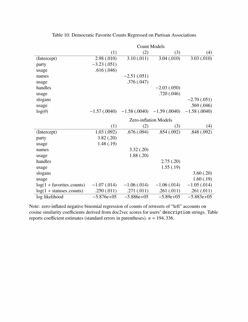
Table 10: Democratic Favorite Counts Regressed on Partisan Associations

Count Models(1) (2) (3) (4)

(Intercept) 2.98 (.010) 3.10 (.011) 3.04 (.010) 3.03 (.010)party −3.23 (.051)usage .616 (.046)names −2.51 (.051)usage .376 (.047)handles −2.03 (.050)usage .720 (.046)slogans −2.70 (.051)usage .569 (.046)log(θ) −1.57 (.0040) −1.58 (.0040) −1.59 (.0040) −1.58 (.0040)

Zero-inflation Models(1) (2) (3) (4)

(Intercept) 1.03 (.092) .676 (.094) .854 (.092) .848 (.092)party 3.82 (.20)usage 1.48 (.19)names 3.32 (.20)usage 1.88 (.20)handles 2.75 (.20)usage 1.55 (.19)slogans 3.60 (.20)usage 1.60 (.19)log(1 + favorites counts) −1.07 (.014) −1.06 (.014) −1.06 (.014) −1.05 (.014)log(1 + statuses counts) .250 (.011) .271 (.011) .261 (.011) .261 (.011)log likelihood −5.876e+05 −5.886e+05 −5.89e+05 −5.883e+05

Note: zero-inflated negative binomial regression of counts of retweets of “left” accounts oncosine similarity coefficients derived from doc2vec scores for users’ description strings. Tablereports coefficient estimates (standard errors in parentheses). n = 194, 336.

Table 11: Republican Favorite Counts Regressed on Partisan Associations

Count Models(1) (2) (3) (4)

(Intercept) 1.59 (.015) 1.46 (.015) 1.56 (.016) 1.60 (.015)party 4.27 (.078)usage 4.21 (.066)names 4.87 (.077)usage 4.25 (.065)handles 4.81 (.076)usage 3.68 (.068)slogans 5.76 (.074)usage 3.40 (.067)log(θ) −2.42 (.0050) −2.41 (.0051) −2.41 (.0050) −2.39 (.0051)

Zero-inflation Models(1) (2) (3) (4)

(Intercept) 1.73 (.14) 1.94 (.14) 1.88 (.14) 1.89 (.14)party −1.77 (.29)usage −3.32 (.27)names −.352 (.28)usage −3.78 (.27)handles −1.31 (.28)usage −3.62 (.28)slogans −3.00 (.27)usage −3.38 (.27)log(1 + favorites counts) −1.00 (.018) −.992 (.017) −1.01 (.018) −1.00 (.017)log(1 + statuses counts) .229 (.016) .212 (.016) .221 (.016) .22 (.016)log likelihood −3.518e+05 −3.514e+05 −3.514e+05 −3.502e+05

Note: zero-inflated negative binomial regression of counts of retweets of “left” accounts oncosine similarity coefficients derived from doc2vec scores for users’ description strings. Tablereports coefficient estimates (standard errors in parentheses). n = 194, 336.

Table 12: Left Favorite Counts Regressed on Partisan Associations

Count Models(1) (2) (3) (4)

(Intercept) 3.65 (.0096) 3.76 (.0099) 3.70 (.0097) 3.69 (.0097)party −3.12 (.047)usage .487 (.042)names −2.53 (.047)usage .235 (.043)handles −2.04 (.047)usage .58 (.042)slogans −2.64 (.047)usage .437 (.043)log(θ) −1.46 (.0035) −1.47 (.0035) −1.48 (.0035) −1.47 (.0035)

Zero-inflation Models(1) (2) (3) (4)

(Intercept) 1.26 (.092) 1.01 (.093) 1.12 (.092) 1.16 (.092)party 3.05 (.20)usage .501 (.19)names 2.51 (.20)usage .778 (.20)handles 2.10 (.20)usage .583 (.19)slogans 2.40 (.20)usage .510 (.19)log(1 + favorites counts) −1.15 (.014) −1.15 (.014) −1.14 (.014) −1.15 (.014)log(1 + statuses counts) .22 (.011) .236 (.011) .228 (.011) .229 (.011)log likelihood −7.134e+05 −7.142e+05 −7.147e+05 −7.141e+05

Note: zero-inflated negative binomial regression of counts of retweets of “left” accounts oncosine similarity coefficients derived from doc2vec scores for users’ description strings. Tablereports coefficient estimates (standard errors in parentheses). n = 194, 336.

Table 13: Right Favorite Counts Regressed on Partisan Associations

Count Models(1) (2) (3) (4)

(Intercept) 2.28 (.012) 2.19 (.011) 2.27 (.012) 2.30 (.011)party 3.56 (.057)usage 3.66 (.050)names 3.63 (.056)usage 3.77 (.049)handles 3.54 (.055)usage 3.35 (.051)slogans 4.56 (.053)usage 3.07 (.050)log(θ) −1.86 (.0040) −1.86 (.0040) −1.86 (.0040) −1.84 (.0040)

Zero-inflation Models(1) (2) (3) (4)

(Intercept) 1.86 (.11) 1.91 (.11) 1.92 (.11) 1.96 (.11)party .105 (.24)usage −1.88 (.22)names 1.01 (.23)usage −1.98 (.22)handles .258 (.23)usage −2.05 (.22)slogans −1.19 (.23)usage −1.95 (.22)log(1 + favorites counts) −1.09 (.015) −1.08 (.015) −1.09 (.015) −1.09 (.015)log(1 + statuses counts) .187 (.013) .178 (.013) .182 (.013) .183 (.013)log likelihood −5.207e+05 −5.205e+05 −5.206e+05 −5.189e+05

Note: zero-inflated negative binomial regression of counts of retweets of “left” accounts oncosine similarity coefficients derived from doc2vec scores for users’ description strings. Tablereports coefficient estimates (standard errors in parentheses). n = 194, 336.

Table 14: Left Hashtag Counts Regressed on Partisan Associations

Count Models(1) (2) (3) (4)

(Intercept) 1.87 (.01) 1.98 (.01) 1.93 (.010) 1.92 (.010)party −3.33 (.049)usage 2.68 (.043)names −2.34 (.049)usage 2.50 (.044)handles −1.63 (.048)usage 2.80 (.044)slogans −2.36 (.047)usage 2.67 (.044)log(θ) −1.39 (.0049) −1.42 (.0048) −1.43 (.0048) −1.41 (.0049)

Zero-inflation Models(1) (2) (3) (4)

(Intercept) 5.20 (.08) 4.91 (.08) 4.94 (.081) 4.98 (.080)party 2.54 (.14)usage −1.26 (.12)names 1.22 (.13)usage −1.04 (.12)handles −.112 (.14)usage −1.02 (.12)slogans .671 (.13)usage −1.15 (.12)log(1 + hashtags counts) −1.27 (.0085) −1.27 (.0085) −1.27 (.0085) −1.27 (.0085)log(1 + statuses counts) −.0141 (.0075) .00836 (.0076) .00634 (.0076) .00516 (.0076)log likelihood −4.547e+05 −4.562e+05 −4.569e+05 −4.561e+05

Note: zero-inflated negative binomial regression of counts of retweets of “left” accounts oncosine similarity coefficients derived from doc2vec scores for users’ description strings. Tablereports coefficient estimates (standard errors in parentheses). n = 194, 336.

Table 15: Right Hashtag Counts Regressed on Partisan Associations

Count Models(1) (2) (3) (4)

(Intercept) 1.48 (.012) 1.34 (.011) 1.41 (.011) 1.45 (.011)party 3.63 (.055)usage 5.19 (.049)names 4.36 (.055)usage 5.29 (.048)handles 4.95 (.054)usage 4.66 (.050)slogans 5.20 (.05)usage 4.55 (.048)log(θ) −1.62 (.0052) −1.61 (.0052) −1.59 (.0052) −1.57 (.0052)

Zero-inflation Models(1) (2) (3) (4)

(Intercept) 4.65 (.082 4.75 (.081) 4.74 (.081) 4.77 (.081)party 1.75 (.13)usage −1.72 (.11)names .476 (.13)usage −1.65 (.11)handles −.202 (.13)usage −1.67 (.12)slogans −.684 (.12)usage −1.6 (.11)log(1 + hashtags counts) −1.21 (.0081) −1.21 (.0081) −1.21 (.0081) −1.21 (.0081)log(1 + statuses counts) .0697 (.0078) .0553 (.0077) .0617 (.0077) .0573 (.0076)log likelihood −4.147e+05 −4.138e+05 −4.127e+05 −4.116e+05

Note: zero-inflated negative binomial regression of counts of retweets of “left” accounts oncosine similarity coefficients derived from doc2vec scores for users’ description strings. Tablereports coefficient estimates (standard errors in parentheses). n = 194, 336.

Table 16: Confusion Matrix for Hostile Usages ClassifierPrecision Recall F1 Score Support

Not Hostile Usage 0.90 0.92 0.91 254Hostile Usage 0.66 0.62 0.63 65

Macro Average 0.78 0.77 0.77 319

Table 17: Correlations Between Not-hostile and Hostile Partisan Associations

not hostile hostileusage names party handles usage names party handles

usage: not hostile 1.00 .075 .17 .10 .67 .10 −.072 −.064names: not hostile 1.00 .58 .69 .17 −.080 .062 −.16party: not hostile 1.00 .52 .087 .0032 −.099 −.020handles: not hostile 1.00 .19 −.078 .0098 −.058usage: hostile 1.00 −.029 −.12 −.039names: hostile 1.00 .019 −.083party: hostile 1.00 −.40handles: hostile 1.00

Note: product-moment correlations between partisan associations computed usinghostility-labeled keywords. n = 194, 336.

Table 18: Correlations Between Agnostic and Hostility-labeled Partisan Associations

not hostileb hostileb

usage names party handles slogans usage names party handlesusagea .98 .10 .15 .11 .11 .75 .12 −.062 −.066namesa .010 .95 .57 .66 .69 .015 −.25 .12 −.14partya .096 .57 .97 .50 .66 .12 .0055 −.16 .014handlesa .11 .68 .50 .98 .71 .22 −.11 .061 −.16slogansa .12 .75 .67 .73 .98 .15 .059 −.0096 −.16

Note: product-moment correlations between partisan associations computed without hostilitylabeling and partisan associations computed using hostility-labeled keywords. n = 194, 336.a partisan associations computed without labeling keywords for hostile usage. b partisanassociations computed with keywords labeled for hostile usage.

Table 19: Congress Following Counts Regressed on Partisan Associations

(a) Republican Members of Congress FollowedCount Models

(1) (2) (3) (4)est SE est SE est SE est SE

(Intercept) −.0567 .026 −.112 .025 −.0909 .025 −.00317 .026diffa 1.53 .075 .478 .071 .672 .069 1.18 .068usage 3.14 .074 3.372 .074 3.24 .075 3.08 .073log(θ) −2.13 .018 −2.16 .018 −2.16 .017 −2.08 .019

Zero-inflation Models(1) (2) (3) (4)

est SE est SE est SE est SE(Intercept) −.915 .081 −1.01 .087 −.960 .082 −.767 .072diffa .0404 .23 .727 .24 1.21 .23 −1.49 .16usage −4.14 .23 −4.38 .26 −4.73 .28 −3.36 .19log likelihood −2.266e+05 −2.268e+05 −2.268e+05 −2.265e+05

(b) Democratic Members of Congress FollowedCount Models

(1) (2) (3) (4)est SE est SE est SE est SE

(Intercept) .686 .011 .773 .011 .71 .011 .699 .011diffa −2.25 .057 −2.25 .056 −1.78 .056 −2.21 .056usage 2.31 .049 2.06 .050 2.28 .049 2.25 .050log(θ) −1.49 .009 −1.50 .0093 −1.55 .0092 −1.51 .0093

Zero-inflation Models(1) (2) (3) (4)

est SE est SE est SE est SE(Intercept) −1.93 .12 −2.40 .13 −1.93 .15 −2.09 .14diffa 7.67 .19 6.89 .18 6.58 .21 6.56 .18usage 3.43 .14 3.77 .15 3.24 .16 3.14 .15log(1 + statuses counts) −.088 .013 −.0556 .014 −.128 .018 −.077 .016log likelihood −3.353e+05 −3.355e+05 −3.363e+05 −3.356e+05

Note: zero-inflated negative binomial regression of counts of members of Congress each userfollows. Table reports coefficient estimates (standard errors in parentheses). n = 194, 336.a partisan association difference variable: (1) party; (2) names; (3) handles; (4) slogans.Partisan associations do not distinguish hostile keyword usages. Estimates using hostility-awarepartisan associations are similar: coefficients for usage are slightly more positive with not-hostilepartisan associations.

Table 20: Congress Following Counts Regressed on Hostile Partisan Associations

(a) Republican Members of Congress FollowedCount Models

(1) (2) (3)est SE est SE est SE

(Intercept) .0601 .018 .0782 .017 .0233 .014diffa −.371 .089 1.39 .095 −.367 .090usage 3.05 .090 3.22 .088 3.20 .085log(θ) −2.35 .0097 −2.33 .011 −2.37 .0072

Zero-inflation Models(1) (2) (3)

est SE est SE est SE(Intercept) −3.11 .28 −3.90 .41 −6.78 1.6diffa 7.37 1.2 −8.94 1.3 17.0 5.5usage −5.65 1.2 −.216 .83 2.19 2.2log likelihood −2.281e+05 −2.279e+05 −2.281e+05

(b) Democratic Members of Congress FollowedCount Models

(1) (2) (3)est SE est SE est SE

(Intercept) .853 .010 .873 .010 .856 .010diffa .879 .062 1.03 .062 .261 .060usage 1.59 .064 1.51 .064 1.48 .064log(θ) −1.73 .0053 −1.72 .0053 −1.73 .0053

Zero-inflation Models(1) (2) (3)

est SE est SE est SE(Intercept) 1.52 .25 1.52 .25 1.57 .25diffa .794 .77 .34 .70 .0845 .68usage 5.37 .73 5.27 .71 5.04 .71log(1 + statuses counts) −.817 .038 −.814 .038 −.817 .038log likelihood −3.384e+05 −3.383e+05 −3.385e+05

Note: zero-inflated negative binomial regression of counts of members of Congress each userfollows. Table reports coefficient estimates (standard errors in parentheses). n = 194, 336.a partisan association difference variable: (1) party; (2) names; (3) handles. Partisanassociations are based on hostile keyword usages.

Table 21: Regressions of Subreddit Identifier on Catenated Comments

r/The Donald r/hillaryclinton

regressor Coef SE Coef SEIntercept −.416 .019 −4.36 .039usage 7.46 .059 10.5 .097party −1.78 .09 −7.87 .16

r/The Donald r/hillaryclinton

regressor Coef SE Coef SEIntercept .200 .021 −3.64 .040usage 7.32 .060 9.75 .096names −8.41 .087 −9.87 .14

r/The Donald r/hillaryclinton

subreddit Coef SE Coef SEIntercept −.351 .020 −4.09 .039usage 7.58 .059 10.9 .098handles −1.81 .081 −7.70 .14

r/The Donald r/hillaryclinton

subreddit Coef SE Coef SEr/The Donald −.345 .019 −4.32 .040r/The Donald 7.71 .059 11.3 .099r/The Donald −3.24 .087 −12.3 .15

Note: multinomial logit regression of subreddit membership on catanated comment vectoraverages and differences. r/pcmasterrace is the reference category. Observations by subreddit:r/The Donald, 207,512; r/hillaryclinton, 11,612; r/pcmasterrace, 26,791.

Table 22: Keyword Frequencies in Novel Descriptions During Each Period

keyword post- up to earlykeyword election election Dec 31 2018trump 2.167 3.813 2.175 2.730clinton .428 .560 .359 .231donald .253 .472 .288 .272hillary .887 1.180 .719 .280republican .404 .487 .399 .385democrat .865 1.114 .846 1.017realdonaldtrump .080 .132 .078 .102hillaryclinton .149 .207 .135 .119maga .797 1.380 .873 2.071strongertogether .098 .138 .083 .051

Note: percentages of initial novel descriptions in each period that contain each keyword string.Number of initial novel descriptions by period: election, 214,458; post-election, 96,055; up toDec 31, 215,164; early 2018, 143,537.

Table 23: Regressions of Novel Description Occurrence on Partisan Associations

(1) (2) (3)election vs election vs up to Dec 31

post-election early 2018 vs early 2018regressor est SE est SE est SEIntercept −.919 .0081 −.337 .0069 −.340 .0069usage .564 .035 −.0722 .031 −.0712 .031party −.197 .039 .0704 .034 .0656 .034

election vs election vs up to Dec 31post-election early 2018 vs early 2018

regressor est SE est SE est SEIntercept −.908 .0081 −.329 .0070 −.332 .0070usage .551 .035 −.0643 .031 −.0638 .031names −.419 .039 −.476 .034 −.478 .034

election vs election vs up to Dec 31post-election early 2018 vs early 2018

regressor est SE est SE est SEIntercept −.916 .0081 −.338 .0069 −.341 .0069usage .534 .035 −.0327 .031 −.0319 .031handles .109 .038 −.299 .033 −.301 .033

election vs election vs up to Dec 31post-election early 2018 vs early 2018

regressor est SE est SE est SEIntercept −.915 .0081 −.342 .0069 −.345 .0069usage .534 .035 −.0307 .031 −.0300 .031slogans .104 .038 −.313 .033 −.315 .033

Note: three multinomial logit regressions of the presence of a novel description during each timeperiod. The first period listed in each column heading is the reference category for the referenttwo-category model.

Figure 1: Timelines and Favorites First and Last Tweet Times

(a) timelines (b) retweets in timelines

(c) favorites

Note: for each user the the earliest Tweet’s time in the retrieved timeline or set of favorites isshown on the x-axis, and the y-axis shows the latest Tweet’s time.

Figure 2: Cosine Similarities for Word Embedding Vector Combinations

(a) usage by party (r = .091) (b) usage by names (r = .0077)

(c) usage by handles (r = .13) (d) usage by slogans (r = .13)

Note: Scatterplots of partisan association average (usage) and difference (party, names,handles, slogans) scores. n = 194, 336. r is the product-moment correlation.

Figure 3: Cosine Similarities for Word Embedding Vector Combinations

(a) party by slogans (r = .64) (b) party by handles (r = .48)

(c) names by party (r = .53) (d) names by slogans (r = .69)

(e) names by handles (r = .65) (f) handles by slogans (r = .72)

Note: Scatterplots of partisan association difference (party, names, handles, slogans) scores.n = 194, 336. r is the product-moment correlation.

Figure 4: Distributions of Retweet, Favorite and Hashtag Counts

Tweets

log(1+Tweets)

Fre

quen

cy

0 5 10 15

010

000

3000

050

000

7000

0

retweets

log(1+retweets)

Fre

quen

cy

2 4 6 8

010

000

2000

030

000

favorites

log(1+favorites)

Fre

quen

cy

0 2 4 6 8 10 12 14

050

0010

000

1500

020

000

2500

0

hashtags

log(1+hashtags)

Fre

quen

cy

0 2 4 6 8

020

000

4000

060

000

8000

012

0000

Democratic retweets

log(1+Democratic retweets)

Fre

quen

cy

0 2 4 6 8

020

000

4000

060

000

8000

0

Republican retweets

log(1+Republican retweets)

Fre

quen

cy

0 2 4 6 8

020

000

6000

010

0000

1400

00

Democratic favorites

log(1+Democratic favorites)

Fre

quen

cy

0 2 4 6 8

020

000

4000

060

000

8000

0

Republican favorites

log(1+Republican favorites)

Fre

quen

cy

0 2 4 6 8

020

000

6000

010

0000

1400

00

left retweets

log(1+left retweets)

Fre

quen

cy

0 2 4 6

0e+

002e

+04

4e+

046e

+04

8e+

041e

+05

right retweets

log(1+right retweets)

Fre

quen

cy

0 2 4 6 8

020

000

6000

010

0000

1400

00

left favorites

log(1+left favorites)

Fre

quen

cy

0 2 4 6 8

020

000

4000

060

000

right favorites

log(1+right favorites)

Fre

quen

cy

0 2 4 6 8

0e+

002e

+04

4e+

046e

+04

8e+

041e

+05

left hashtags

log(1+left hashtags)

Fre

quen

cy

0 2 4 6 8

050

000

1000

0015

0000

2000

00

right hashtags

log(1+right hashtags)

Fre

quen

cy

0 2 4 6 8

050

000

1000

0015

0000

2000

00

Note: histograms of log counts of Tweets (statuses), retweets, favorites or hastags in users’timelines.

Figure 5: Coefficients from Regressions of Retweets, Likes and Hashtags on Partisan Associations

(a) count model: differences (b) count model: usage

−4

−2

02

46

coef

ficie

nt

●●

●

●

●

●

●

●

●●

Rp Fp

Rp Fp

Rp FpHp

Rp

Fp Hp

●●

●

●

●

●

●

●

●

●

Rn Fn

Rn

Fn

Rn FnHn

Rn

Fn

Hn

●

●

●

●

●

●

●

●

●

●

RhFh

Rh

Fh

Rh FhHh

Rh

Fh

Hh

●●

●

●

● ●

●

●

●

●

Rs Fs

Rs

Fs

Rs FsHs

Rs

Fs

Hs

−4

−2

02

46

coef

ficie

nt

●

●

●

●

●

●

●

●

●●

●

●

● ●

●

●

●

●●

●

●

●●

●

●

●

●

●

● ●

●

● ●

●

●

●

●●

●

●

RuRuRuRu

FuFuFuFu

RuRuRu

Ru

FuFu

FuFu

RuRuRuRu

FuFuFuFu

HuHuHuHu

RuRu

RuRuFuFu

FuFu

HuHu

HuHu

(c) zero-inflated model: differences (d) zero-inflated model: usage

−4

−2

02

46

coef

ficie

nt

●

●

●

●

●

●

●

●

●

●

Rp

Fp

Rp

Fp

Rp

FpHp

Rp

Fp

Hp

●

●

● ●

●

●

●

●

●

●

Rn

Fn

RnFn

Rn

Fn

Hn

Rn

FnHn

●

●

●

●

●

●

●

●

●

●

Rh

Fh

Rh

Fh

Rh

Fh

Hh

Rh

FhHh

●

●

●

●

●

●

●

●

●

●

Rs

Fs

Rs

Fs

Rs

Fs

Hs

Rs

Fs

Hs

−4

−2

02

46

coef

ficie

nt

●

●

● ●

●

●●

●

●

●

●

●

●

●

●

●

●

●●

●

●

●●

●

●

●

●

●

●

●●

●

●●

●●

●●

●●

Ru

RuRuRuFu

FuFuFu

RuRu

RuRu

Fu

FuFu

Fu

Ru

RuRuRu

FuFuFuFu

HuHu

HuHu

RuRuRu

Ru

FuFuFuFu

HuHuHuHu

Note: coefficients with 95% confidence intervals from zero-inflated negative binomial countmodels using partisan association regressors (also Tweet counts and retweets, likes or hashtagscounts variables in the zero-inflated models).Color legend: blue, Democratic; red, Republican; green, left; orange, right.Letter legend: R, retweet; F, favorite (like); H, hashtag; p, party; n, names; h, handles; s, slogans;u, usage.

Figure 6: Distribution of the Names Partisan Association Scores of users who used given out-of-sample words

(a) party (b) names

(c) handles (d) slogans

Note: distributions of partisan association scores for users whose descriptions include“ImWithHer”,” “NeverTrump” or “MakeAmericaGreatAgain.”

Figure 7: Not-hostile by Hostile Word Embedding Vector Combinations

(a) party (r = −.099) (b) names (r = −.080)

(c) handles (r = −.058) (d) usage (r = .67)

Note: Scatterplots of not-hostile versus hostile partisan association average (usage) anddifference (party, names, handles) scores. n = 194, 336. r is the product-moment correlation.