passive control of aerodynamic load in wind turbine … · passive control of aerodynamic load in...
TRANSCRIPT

Passive Control of Aerodynamic Load in Wind TurbineBlades
Edgar Sousa Carrolo
Thesis to obtain the Master of Science Degree in
Aerospace Engineering
Supervisor: Professor André Calado Marta
Examination Committee
Chairperson: Professor Filipe Szolnoky Ramos Pinto CunhaSupervisor: Professor André Calado MartaMember of the Committee: Doctor José Lobo do Vale
June 2015

ii

Acknowledgments
I would like to give a word of gratitude in first place, to my supervisor Andre Marta for his total availability
whenever I needed. He trusted in me since the beginning and gave me all the confidence to overcome
the difficulties I had throughout this work. Thank you for everything! The greeting is extended to the Ph
D. student Simao Rodrigues for his technical tips and advices.
I want to thank my dear friends and colleagues Jose and Diogo, for their concern about my progress
and emotional support, not only during the dissertation period but all the university time. All those who
always cared about me are also included.
Finally, I want to thank my family, whose financial support was crucial. They never put pressure on
me, and gave me freedom to follow my own path, always demonstrating their confidence on me. I hope,
from now on, through the working tool you gave me opportunity to get, reward all the effort you done in
my education ever since.
iii

iv

Resumo
As pas de turbinas eolicas com grandes dimensoes tem muitas vantagens em termos de eficiencia
energetica, no entanto o seu dimensionamento representa um maior desafio, devido as elevadas cargas
a que estas estruturas estao sujeitas.
Tradicionalmente, os sistemas de controlo activo permitem a pa adaptar-se de acordo com as
condicoes de vento, e assim manter a sua eficiencia dentro de nıveis aceitaveis. Desde o final do
seculo passado, alguns investigadores tem vindo a discutir acerca de tecnicas de controlo passivo.
A implementacao deste tipo de resposta aerolastica nao introduz peso ou manutencao adicional, ao
contrario do controlo activo, porque nao existem estruturas adicionais ou complementares, e e muito
util para a reducao de cargas de fadiga ou optimizar a energia produzida. O objectivo passou por
conseguir uma reducao efectiva da carga aerodinamica num modelo computacional de uma pa. No
ambito deste trabalho foram desenvolvidos modelos computacionais que simulam a interaccao fluıdo-
estrutura num modelo de pa aperfeicoado, e foi considerado inicialmente num analise acoplada, apenas
a carga aerodinamica e de seguida, combinando-a com carregamentos inerciais. Os resultados demon-
straram que este design reduzir em 2.1% a carga aerodinamica na condicao de um vento de velocidade
maxima de operacao. Uma validacao estatica preliminar foi realizada com sucesso, tendo em conta
valores maximos de referencia.
Palavras-chave: Adaptacao aeroelastica, Acoplamento flexao-torcao, Controlo passivo, Car-
regamento aerodinamico, Interacao fluido-estrutura.
v

vi

Abstract
Large wind turbine blades have many advantages in terms of power efficiency, despite representing an
hazard concerning the high loads applied on the structure. Traditionally, there are active control sys-
tems that allow blades to adapt according to wind conditions, and so maintain power efficiency and
aerodynamic load within acceptable levels. Since the end of the last century, some researchers have
been discussing about passive control techniques. The implementation of this kind of aeroelastic re-
sponse does not bring additional maintenance or weight, unlike active control, because there are no
additional devices or complementary structures, and is very useful either to reduce fatigue loads or op-
timize energy output. The main purpose was to achieve an effective reduction in aerodynamic loading
in a wind turbine blade. In the scope of this work, computational models were developed that simulated
the fluid-structure interaction on a enhanced blade model. Coupled analysis considering first only the
aerodynamic load and then combining it with inertial were performed. The results demonstrated that
this design could reduce 2.1% aerodynamic load in high wind speeds at the cut-out wind speed, thus
proving to be a realistic passive control technique. A preliminary static validation of the enhanced blade
model was successfully done, taking into account maximum reference values.
Keywords: Aeroelastic Tailoring, Bend-twist Coupling, Passive Control, Aerodynamic Load,
Fluid- structure Interaction.
vii

viii

Contents
Acknowledgments . . . . . . . . . . . . . . . . . . . . . . . . . . . . . . . . . . . . . . . . . . . iii
Resumo . . . . . . . . . . . . . . . . . . . . . . . . . . . . . . . . . . . . . . . . . . . . . . . . . v
Abstract . . . . . . . . . . . . . . . . . . . . . . . . . . . . . . . . . . . . . . . . . . . . . . . . . vii
List of Tables . . . . . . . . . . . . . . . . . . . . . . . . . . . . . . . . . . . . . . . . . . . . . . xiii
List of Figures . . . . . . . . . . . . . . . . . . . . . . . . . . . . . . . . . . . . . . . . . . . . . xvii
Nomenclature . . . . . . . . . . . . . . . . . . . . . . . . . . . . . . . . . . . . . . . . . . . . . . xxi
Glossary . . . . . . . . . . . . . . . . . . . . . . . . . . . . . . . . . . . . . . . . . . . . . . . . xxiii
1 Introduction 1
1.1 Motivation . . . . . . . . . . . . . . . . . . . . . . . . . . . . . . . . . . . . . . . . . . . . . 1
1.2 Wind Energy Overview . . . . . . . . . . . . . . . . . . . . . . . . . . . . . . . . . . . . . . 2
1.2.1 Historic Perspective . . . . . . . . . . . . . . . . . . . . . . . . . . . . . . . . . . . 2
1.2.2 Modern Wind Energy Context . . . . . . . . . . . . . . . . . . . . . . . . . . . . . . 4
1.3 Objectives . . . . . . . . . . . . . . . . . . . . . . . . . . . . . . . . . . . . . . . . . . . . . 6
1.4 Thesis Outline . . . . . . . . . . . . . . . . . . . . . . . . . . . . . . . . . . . . . . . . . . 6
2 Horizontal-Axis Wind Turbines 7
2.1 Generic Overview . . . . . . . . . . . . . . . . . . . . . . . . . . . . . . . . . . . . . . . . 7
2.2 Sources of Load on Blades . . . . . . . . . . . . . . . . . . . . . . . . . . . . . . . . . . . 8
2.3 Power and Torque Characteristics . . . . . . . . . . . . . . . . . . . . . . . . . . . . . . . 8
2.4 Blade Design and Properties . . . . . . . . . . . . . . . . . . . . . . . . . . . . . . . . . . 9
2.4.1 Blade Section . . . . . . . . . . . . . . . . . . . . . . . . . . . . . . . . . . . . . . . 9
2.4.2 Blade Material Properties . . . . . . . . . . . . . . . . . . . . . . . . . . . . . . . . 9
2.4.3 Airfoil Optimization . . . . . . . . . . . . . . . . . . . . . . . . . . . . . . . . . . . . 11
2.4.4 Number of Blades . . . . . . . . . . . . . . . . . . . . . . . . . . . . . . . . . . . . 11
2.4.5 Blade Twist Design . . . . . . . . . . . . . . . . . . . . . . . . . . . . . . . . . . . . 12
2.4.6 Blade Thickness . . . . . . . . . . . . . . . . . . . . . . . . . . . . . . . . . . . . . 13
2.4.7 Tip-Speed Ratio . . . . . . . . . . . . . . . . . . . . . . . . . . . . . . . . . . . . . 13
3 Aerodynamic Load Control 15
3.1 Active Load Control . . . . . . . . . . . . . . . . . . . . . . . . . . . . . . . . . . . . . . . 15
3.1.1 Variable Pitch Angle Blades . . . . . . . . . . . . . . . . . . . . . . . . . . . . . . 16
ix

3.1.2 Active Flow Control Techniques . . . . . . . . . . . . . . . . . . . . . . . . . . . . . 16
3.2 Passive Load Control . . . . . . . . . . . . . . . . . . . . . . . . . . . . . . . . . . . . . . 17
3.2.1 Stall Regulation . . . . . . . . . . . . . . . . . . . . . . . . . . . . . . . . . . . . . 17
3.2.2 Aerolastic Tailoring . . . . . . . . . . . . . . . . . . . . . . . . . . . . . . . . . . . . 18
3.2.3 Bend-Twist Coupling . . . . . . . . . . . . . . . . . . . . . . . . . . . . . . . . . . . 18
4 Aerodynamic Model 22
4.1 Incompressible Potential Flow Fundamentals . . . . . . . . . . . . . . . . . . . . . . . . . 22
4.1.1 Boundary Conditions . . . . . . . . . . . . . . . . . . . . . . . . . . . . . . . . . . . 24
4.1.2 Vortex Flow . . . . . . . . . . . . . . . . . . . . . . . . . . . . . . . . . . . . . . . . 25
4.1.3 Actuator Disk Concept . . . . . . . . . . . . . . . . . . . . . . . . . . . . . . . . . . 25
4.1.4 Classical Blade Element Method Theory . . . . . . . . . . . . . . . . . . . . . . . . 27
4.2 Numerical Models . . . . . . . . . . . . . . . . . . . . . . . . . . . . . . . . . . . . . . . . 29
4.2.1 Panel Method . . . . . . . . . . . . . . . . . . . . . . . . . . . . . . . . . . . . . . . 29
4.2.2 BEM Iterative Solution . . . . . . . . . . . . . . . . . . . . . . . . . . . . . . . . . . 30
4.3 Description of Aerodynamic Routine Program aero load.m . . . . . . . . . . . . . . . . . . 32
4.3.1 Purpose and Objectives . . . . . . . . . . . . . . . . . . . . . . . . . . . . . . . . 32
4.3.2 Input Variables . . . . . . . . . . . . . . . . . . . . . . . . . . . . . . . . . . . . . . 32
4.3.3 Pressure distribution . . . . . . . . . . . . . . . . . . . . . . . . . . . . . . . . . . . 33
4.3.4 BEM Computation . . . . . . . . . . . . . . . . . . . . . . . . . . . . . . . . . . . . 33
4.4 Aerodynamic Load Computation . . . . . . . . . . . . . . . . . . . . . . . . . . . . . . . . 34
4.4.1 Program Routine . . . . . . . . . . . . . . . . . . . . . . . . . . . . . . . . . . . . . 35
5 Structural Model 37
5.1 Linear Elasticity Foundations . . . . . . . . . . . . . . . . . . . . . . . . . . . . . . . . . . 37
5.2 Finite Element Matrix Formulation . . . . . . . . . . . . . . . . . . . . . . . . . . . . . . . 38
5.3 Composite materials . . . . . . . . . . . . . . . . . . . . . . . . . . . . . . . . . . . . . . . 40
5.4 Description of Structural Mesh Generator WTB struct model.m . . . . . . . . . . . . . . . 41
5.4.1 Purposes and Objectives . . . . . . . . . . . . . . . . . . . . . . . . . . . . . . . . 41
5.4.2 Input Variables . . . . . . . . . . . . . . . . . . . . . . . . . . . . . . . . . . . . . . 42
5.4.3 Nodes Assembly . . . . . . . . . . . . . . . . . . . . . . . . . . . . . . . . . . . . . 42
5.4.4 Elements Assembly . . . . . . . . . . . . . . . . . . . . . . . . . . . . . . . . . . . 43
5.5 Load and Nodal Constraints Computation . . . . . . . . . . . . . . . . . . . . . . . . . . . 44
6 Fluid-Structure Interaction 45
6.1 Fluid Structure Interaction Methods . . . . . . . . . . . . . . . . . . . . . . . . . . . . . . . 45
6.2 Loose Coupling FSI Schemes . . . . . . . . . . . . . . . . . . . . . . . . . . . . . . . . . . 46
6.3 Simplified Coupling Procedure . . . . . . . . . . . . . . . . . . . . . . . . . . . . . . . . . 48
x
7 Parametric Study 51
7.1 Wind Turbine NREL 5 MW Data . . . . . . . . . . . . . . . . . . . . . . . . . . . . . . . . . 51
7.2 Baseline Blade Parameters . . . . . . . . . . . . . . . . . . . . . . . . . . . . . . . . . . . 52
7.3 Baseline Results . . . . . . . . . . . . . . . . . . . . . . . . . . . . . . . . . . . . . . . . . 55
7.3.1 Structural Performance . . . . . . . . . . . . . . . . . . . . . . . . . . . . . . . . . 55
7.3.2 Aerodynamic Performance . . . . . . . . . . . . . . . . . . . . . . . . . . . . . . . 57
7.4 Fibres Orientation . . . . . . . . . . . . . . . . . . . . . . . . . . . . . . . . . . . . . . . . 57
7.5 Thickness Distribution . . . . . . . . . . . . . . . . . . . . . . . . . . . . . . . . . . . . . . 61
7.6 Shear Webs Location . . . . . . . . . . . . . . . . . . . . . . . . . . . . . . . . . . . . . . 64
7.7 Material Reinforcement . . . . . . . . . . . . . . . . . . . . . . . . . . . . . . . . . . . . . 66
7.8 Parametric Study Summary . . . . . . . . . . . . . . . . . . . . . . . . . . . . . . . . . . . 69
8 Enhanced Blade Design 71
8.1 Design properties . . . . . . . . . . . . . . . . . . . . . . . . . . . . . . . . . . . . . . . . 71
8.2 Coupled Analysis . . . . . . . . . . . . . . . . . . . . . . . . . . . . . . . . . . . . . . . . . 72
8.2.1 Structural Performance . . . . . . . . . . . . . . . . . . . . . . . . . . . . . . . . . 72
8.3 Aerodynamic Performance . . . . . . . . . . . . . . . . . . . . . . . . . . . . . . . . . . . 75
8.4 Static Analysis including Inertial Loads . . . . . . . . . . . . . . . . . . . . . . . . . . . . . 75
9 Conclusions 79
9.1 Achievements . . . . . . . . . . . . . . . . . . . . . . . . . . . . . . . . . . . . . . . . . . . 80
9.2 Future Work . . . . . . . . . . . . . . . . . . . . . . . . . . . . . . . . . . . . . . . . . . . . 80
Bibliography 84
A 85
A.1 von Mises Failure Criterion . . . . . . . . . . . . . . . . . . . . . . . . . . . . . . . . . . . 85
A.2 Thin Airfoil Theory . . . . . . . . . . . . . . . . . . . . . . . . . . . . . . . . . . . . . . . . 85
B 88
B.1 Matlab APDL Code Generator . . . . . . . . . . . . . . . . . . . . . . . . . . . . . . . . . 88
xi

xii

List of Tables
7.1 NREL MW wind turbine specifications [1]. . . . . . . . . . . . . . . . . . . . . . . . . . . . 52
7.2 NREL 5MW wind turbine blade airfoils [1]. . . . . . . . . . . . . . . . . . . . . . . . . . . . 52
7.3 Modified airfoil sections. . . . . . . . . . . . . . . . . . . . . . . . . . . . . . . . . . . . . . 52
7.4 Blade geometrical data [2]. . . . . . . . . . . . . . . . . . . . . . . . . . . . . . . . . . . . 53
7.5 Mechanical properties of fibre glass and epoxy [3], [4]. . . . . . . . . . . . . . . . . . . . . 53
7.6 E-glass/Epoxy composite mechanical properties [5]. . . . . . . . . . . . . . . . . . . . . . 53
7.7 Baseline maximum values. . . . . . . . . . . . . . . . . . . . . . . . . . . . . . . . . . . . 56
7.8 Layers orientation; maximum values. . . . . . . . . . . . . . . . . . . . . . . . . . . . . . . 58
7.9 Multi-directional Laminates stack. . . . . . . . . . . . . . . . . . . . . . . . . . . . . . . . . 58
7.10 Thickness distribution; maximum values . . . . . . . . . . . . . . . . . . . . . . . . . . . . 62
7.11 Number of webs; maximum values. . . . . . . . . . . . . . . . . . . . . . . . . . . . . . . . 64
7.12 Carbon(T300)/epoxy composite mechanical properties [5]. . . . . . . . . . . . . . . . . . . 66
7.13 Material reinforcement; maximum values . . . . . . . . . . . . . . . . . . . . . . . . . . . . 67
8.1 Enhanced blade: maximum values. . . . . . . . . . . . . . . . . . . . . . . . . . . . . . . . 74
8.2 Enhanced blade: parameters deviations between first and last iterations. . . . . . . . . . . 75
xiii

xiv

List of Figures
1.1 Windmill from the 18th century in Northern Holland [6]. . . . . . . . . . . . . . . . . . . . . 2
1.2 Wind turbine from Paul La Cour [7]. . . . . . . . . . . . . . . . . . . . . . . . . . . . . . . . 3
1.3 Wind turbine size evolution [8]. . . . . . . . . . . . . . . . . . . . . . . . . . . . . . . . . . 5
1.4 Global wind energy capacity [8]. . . . . . . . . . . . . . . . . . . . . . . . . . . . . . . . . 5
2.1 Main components of a wind turbine blade [9]. . . . . . . . . . . . . . . . . . . . . . . . . . 7
2.2 Example of blade internal structure with two shear webs[7]. . . . . . . . . . . . . . . . . . 9
2.3 Blade sections. . . . . . . . . . . . . . . . . . . . . . . . . . . . . . . . . . . . . . . . . . . 10
2.4 Evolution in power efficiency [7]. . . . . . . . . . . . . . . . . . . . . . . . . . . . . . . . . 11
2.5 Power efficiency vs. tip speed ratio for different number of blades [7]. . . . . . . . . . . . . 12
2.6 Twist vs Relative blade length ; power coefficient vs tip speed ratio for three different
twisted blades [7]. . . . . . . . . . . . . . . . . . . . . . . . . . . . . . . . . . . . . . . . . 13
3.1 Pitch towards feather and stall [7]. . . . . . . . . . . . . . . . . . . . . . . . . . . . . . . . 16
3.2 Partial active pitch-controlled blade [7]. . . . . . . . . . . . . . . . . . . . . . . . . . . . . . 17
3.3 Comparison of a) conventional blade; b) bending-twist coupled blade [10]. . . . . . . . . . 19
4.1 Circulation [11]. . . . . . . . . . . . . . . . . . . . . . . . . . . . . . . . . . . . . . . . . . . 22
4.2 Schematic representation of a vortex [11]. . . . . . . . . . . . . . . . . . . . . . . . . . . . 23
4.3 Infinity and wall boundary conditions [12]. . . . . . . . . . . . . . . . . . . . . . . . . . . . 24
4.4 Vortex [11]. . . . . . . . . . . . . . . . . . . . . . . . . . . . . . . . . . . . . . . . . . . . . 25
4.5 Schematic representation of 1-D wind turbine blade [9]. . . . . . . . . . . . . . . . . . . . 26
4.6 Wake rotation [13]. . . . . . . . . . . . . . . . . . . . . . . . . . . . . . . . . . . . . . . . . 27
4.7 Domain control volume [14]. . . . . . . . . . . . . . . . . . . . . . . . . . . . . . . . . . . . 28
4.8 Schematic represetation of aerodynamic angles [14]. . . . . . . . . . . . . . . . . . . . . 28
4.9 Surface discretization by panels [12]. . . . . . . . . . . . . . . . . . . . . . . . . . . . . . . 29
4.10 Numerical incompatibility in trailing edge [12]. . . . . . . . . . . . . . . . . . . . . . . . . . 30
4.11 Fluxogram about BEM iterative solution. . . . . . . . . . . . . . . . . . . . . . . . . . . . . 32
4.12 Fluxogram about aerodynamic model framework. . . . . . . . . . . . . . . . . . . . . . . . 35
5.1 4-nodded shell element [15]. . . . . . . . . . . . . . . . . . . . . . . . . . . . . . . . . . . 39
5.2 A stack with various unidirectional layers [16]. . . . . . . . . . . . . . . . . . . . . . . . . . 41
xv

5.3 Airfoil section computation. . . . . . . . . . . . . . . . . . . . . . . . . . . . . . . . . . . . 42
5.4 Mesh example. . . . . . . . . . . . . . . . . . . . . . . . . . . . . . . . . . . . . . . . . . . 43
5.5 Assembled elements. . . . . . . . . . . . . . . . . . . . . . . . . . . . . . . . . . . . . . . 44
6.1 Exchange domain between aerodynamic and structural models. . . . . . . . . . . . . . . 45
6.2 FSI coupling level [17]. . . . . . . . . . . . . . . . . . . . . . . . . . . . . . . . . . . . . . . 46
6.3 Static loose coupling FSI model [18]. . . . . . . . . . . . . . . . . . . . . . . . . . . . . . . 47
6.4 Sobreposition between aerodynamic and structural grid [17]. . . . . . . . . . . . . . . . . 48
6.5 Fluid-structure interaction iterative solution. . . . . . . . . . . . . . . . . . . . . . . . . . . 49
7.1 Fibres orientation. . . . . . . . . . . . . . . . . . . . . . . . . . . . . . . . . . . . . . . . . 54
7.2 Pressure distribution on blade surface. . . . . . . . . . . . . . . . . . . . . . . . . . . . . . 54
7.3 Baseline deformation. . . . . . . . . . . . . . . . . . . . . . . . . . . . . . . . . . . . . . . 55
7.4 Baseline displacement and twist distribution. . . . . . . . . . . . . . . . . . . . . . . . . . 55
7.5 Baseline von Mises equivalent stress. . . . . . . . . . . . . . . . . . . . . . . . . . . . . . 56
7.6 Baseline aerodynamic performance. . . . . . . . . . . . . . . . . . . . . . . . . . . . . . . 57
7.7 Twist distribution for different fibres orientation. . . . . . . . . . . . . . . . . . . . . . . . . 58
7.8 Flapwise displacement at (x/c) = 25% for different fibres orientation. . . . . . . . . . . . . 59
7.9 Edgewise displacement at (x/c) = 25% for different fibres orientation. . . . . . . . . . . . 59
7.10 von Mises equivalent stress distribution: unidirectional stacks. . . . . . . . . . . . . . . . . 60
7.11 von Mises equivalent stress distribution: multidirectional stacks. . . . . . . . . . . . . . . . 61
7.12 Variable thickness distributions. . . . . . . . . . . . . . . . . . . . . . . . . . . . . . . . . 62
7.13 Edgewise displacement at (x/c) = 25% for different thickness distributions. . . . . . . . . 62
7.14 Flapwise displacement at (x/c) = 25% for different thickness distributions. . . . . . . . . . 63
7.15 Twist distribution for different thickness distributions. . . . . . . . . . . . . . . . . . . . . . 63
7.16 von Mises equivalent stress for different thickness distributions. . . . . . . . . . . . . . . . 64
7.17 Edgewise displacement at (x/c) = 25% for different different number of webs. . . . . . . . 65
7.18 Flapwise displacement at (x/c) = 25% for different different number of webs. . . . . . . . 65
7.19 Twist distribution for different number of webs. . . . . . . . . . . . . . . . . . . . . . . . . . 65
7.20 von Mises equivalent stress distribution: number of webs. . . . . . . . . . . . . . . . . . . 66
7.21 Laminate stack with carbon(T300)/epoxy reinforcement. . . . . . . . . . . . . . . . . . . . 67
7.22 Flapwise displacement at (x/c) = 25%. . . . . . . . . . . . . . . . . . . . . . . . . . . . . . 67
7.23 Edgewise displacement at (x/c) = 25% for material reinforcement. . . . . . . . . . . . . . 68
7.24 Twist distribution. . . . . . . . . . . . . . . . . . . . . . . . . . . . . . . . . . . . . . . . . . 68
7.25 von Mises stress distribution: material reinforcement. . . . . . . . . . . . . . . . . . . . . . 68
8.1 Laminate stacks in different blade regions. . . . . . . . . . . . . . . . . . . . . . . . . . . . 72
8.2 Enhanced blade: edgewise displacement at (x/c) = 25%. . . . . . . . . . . . . . . . . . . 73
8.3 Enhanced blade: flapwise displacement displacement at (x/c) = 25%. . . . . . . . . . . . 73
8.4 Enhanced blade: twist distribution. . . . . . . . . . . . . . . . . . . . . . . . . . . . . . . . 73
xvi

8.5 Enhanced blade: von Mises stress plot. . . . . . . . . . . . . . . . . . . . . . . . . . . . . 74
8.6 Enhanced blade: lift coefficient. . . . . . . . . . . . . . . . . . . . . . . . . . . . . . . . . . 75
8.7 Enhanced blade: power coefficient. . . . . . . . . . . . . . . . . . . . . . . . . . . . . . . . 76
8.8 Enhanced blade including inertial loads: flapwise displacement at (x/c) = 25%. . . . . . . 76
8.9 Enhanced blade including inertial loads: edgewise displacement at (x/c) = 25%. . . . . . 77
8.10 Enhanced blade including inertial loads: twist distribution. . . . . . . . . . . . . . . . . . . 77
8.11 Enhanced blade including inertial loads: von Mises stress. . . . . . . . . . . . . . . . . . . 78
A.1 Main airfoil geometric definitions (reproduced from [19]). . . . . . . . . . . . . . . . . . . . 85
A.2 Aerodynamic forces: lift and drag (reproduced from [19]). . . . . . . . . . . . . . . . . . . 87
xvii

xviii

Nomenclature
Greek symbols
α Angle of attack.
β Twist angle.
Γ Circulation.
λ Tip speed ratio.
λr Tip speed ratio in position r of the blade span.
ν Poisson ratio.
Ω Rotor rotational speed.
ω Flow rotation speed.
Φ Potential function.
Ψ Stream function.
ρ Air density.
σ Solidity ratio.
σy Yield strength.
σeqv von Mises equivalent stress.
σUCS Ultimate compressive strength.
θ Pitch angle.
θ0 Design pitch angle.
θa.c. Pitch angle due to active control systems
Π Total potential energy.
σ Stress vector field.
ε Strain vector field.
xix

Roman symbols
[K] Stiffness matrix.
[E] Material elastic matrix.
[G] Gyroscopic matrix, shear modulus
[M ] Mass matrix.
m Mass flow rate.
a Axial induction factor.
B Number of blades.
c Chord.
CP Power coefficient.
Cp Pressure coefficient.
E Young’s modulus.
Ef Composite fibre Young’s modulus.
EI Bending stiffness.
F Force.
GJ Torsional stiffness.
h Thermal expansion vector.
kb Bending curvature.
kt Rate of twist.
Mb Bending moment.
Mt Torsional moment.
P Power.
p0 Atmospheric pressure.
q Nodal displacement vector.
R Rotor radius.
r Rotor radial position.
S Blade wetted surface.
T Torque, Temperature.
xx

U Free-stream wind speed.
u Displacement vector field.
V Fraction in volume, velocity in a flow field in an arbitrary point .
Vrel Relative velocity.
Subscripts
a Aerodynamic.
f Composite fibre.
g Gravity.
l.e. Leading edge.
m Composite matrix.
n.l. Non-linear.
t.e. Trailing edge.
Superscripts
G Global reference frame.
k Iteration number.
S Surface.
T Transpose.
t Thermal.
V Volume.
xxi

xxii

Glossary
BEM Blade Element Method is a 2D classical
method to determine aerodynamic coefficients
and forces applied on a blade annular element.
BTC Bend-Twist Coupling is the elastic coupling
between bending and torsion in composite
structures, similar to beams, governed by the
anisotropic properties of composite materials.
CFD Computational Fuid Dynamics is the computa-
tional fluid mechanics field that uses numerical
tools in to solve fluid flow problems.
CSM Computational Structural Mechanics is the
structural engineering field that applies numeri-
cal methods to solve structural problems, either
static or dynamic.
FEM Finite Element Method is a numerical method
to find approximate solutions of partial differ-
ential equations dividing the domain in smaller
parts called finite elements.
FSI Fluid-Structure Interaction is the interaction of
deformable or moving bodies emerged in a
fluid flow creating steady or oscillatory pertur-
bations.
HAWT Horizontal-Axis Wind Turbines are the most
common configuration of wind rotors, where the
rotation axis is parallel to the ground.
xxiii

xxiv

Chapter 1
Introduction
1.1 Motivation
Along the History, the way humanity has been looking at wind energy has suffered several mutations.
During many centuries, the use of wind energy was limited to charge low-power systems at home, but as
soon as electrical grid became available, wind energy was quickly replaced. Nevertheless, there were
some sparse applications of wind turbines, essentially in Europe, where some avant-garde scientists
wanted to be noticed in this area and contributed with their ideas. Until the last quarter of the twentieth
century, there was in general, little interest to invest in this area.
Since then, several factors have contributed to the way in which we look at wind energy. The dra-
matic rise of oil price forced all entities to seek for alternatives. Wind energy seemed to be a logical
investment, since it had been used in the past in farms (windmills were used to transform wind energy
into mechanical energy), and given that wind is available anywhere on Earth. Furthermore, in that time
developments were made in the technological field, as well as in others, that were significant enough
to sustain the investment and revolutionize wind turbines. These factors, associated with adequate
government policies, contributed to proliferate these devices throughout Europe and North America.
The 1900s enhanced the concern about global warming, from which resulted in a strong demand for
wind power generation. The wind turbines of that time had some technical issues, which were limiting
production quality, but actually there was not a big concern to correct them. The increasing size of wind
turbines caused new advances in many scientific areas, such as aerodynamic, material sciences and
energy conversion, in order to supply the electrical needs of the 21st century. The production costs
dropped in such a way that it became very competitive in comparison with conventional energy sources.
Nowadays, wind turbines are more reliable and cost effective, however, the development in this area
is not over and there are still many opportunities to explore, with the consciousness that the expansion
will bring more issues to overcome.
With design focus on turbine mass and cost for a given performance, it is important to include pas-
sive and active techniques to load control, thereby achieve an overall benefit to the system through
improvements in turbine performance and mitigating both stress and load on the structure.
1

The present work aims to give an additional relevant contribution to the wind energy area and, in
particular, to understand how it is possible to give a response - from a structural point of view - to the
increasing size of the wind turbine blades. In this context, this report will try to give some clues on what
parameters contribute the most to the structural performance of wind turbine blades and, whenever
possible, change them in order to improve the structural performance, specially in situations with high
wind speeds, such as gusts or wind storms.
1.2 Wind Energy Overview
1.2.1 Historic Perspective
It is unanimous that windmills served as an inspiration source to develop wind turbines. There are a few
descriptions about the usage of windmills B.C., although they are not sufficiently documented. In fact,
windmills came to North Europe for the first time between the 10th and 12th century, they all had an
horizontal axis and were used in almost every mechanical task, but mainly for water pumping, grinding
grain and as mechanical tools [9]. An example is illustrated in figure 1.1.
Figure 1.1: Windmill from the 18th century in Northern Holland [6].
Until the industrial revolution, wind was the main source of energy, and only in Europe were installed
about 200 000 windmill, with Germany and Netherlands leading. From technical and technological
developments those devices had already some aerodynamic sophistications. Blades acquired airfoil like
shapes and twist was included. Moreover, rudimentary system of yaw control were implemented. One
of the biggest developments occurred in 18th century, when the British John Smeaton discovered three
basic rules that are still updated in wind energy projects [9].
• The speed of the blade tips is ideally proportional to the wind speed;
• The maximum torque is proportional to the wind speed squared;
• The maximum power is proportional to the wind speed cubed.
After the industrial revolution, coal progressively assumed the role played by windmills. It had great
advantages regarding transportation, since it is possible to move coal to anywhere needed. Further-
more, coal gives the chance to adapt output power according to the actual load, contrasting with what
2

happens in wind energy where there is a direct dependence between output power and wind speed.
The trend of decrease in number of windmills was reinforced with the appearance of the electric grid.
The factories considered that wind energy was an obsolete source of energy and the maintenance costs
of windmills made people invest in steam engines and electricity as main sources of energy.
In the end of the 19th century, a Danish Professor called Paul La Cour gave a great contribution to
wind energy, by converting wind kinetic energy into electrical energy for the first time, based on principles
he developed himself [9]. He inclusively developed his own model, show on figure 1.2.
Figure 1.2: Wind turbine from Paul La Cour [7].
The oil crisis during the 1st World War became an excellent opportunity to spread wind turbines in
Europe. Turbines had up to 20 m height and the output power varied between 10 and 35 kW. However,
the investment dropped some years later due to the decrease in price of diesel, until the 2nd World
War. Even though, this gap in investment allowed an accumulation of technical knowledge, that resulted
in a quite important publication in 1925 by the physicist Albert Betz, where he proved that in a simple
representation of a turbine by a shaped disk, the maximum power coefficient possible to achieve is 59.3
% [13]. This result is still valid in the present days . This kind of progress allowed improvements in rotors
aerodynamics, combined with advances in material science done in aircraft industry.
In the 1950s another stable period in oil prices reigned, which along with intensive programs adopted
by governments to spread electricity in rural areas, discouraged the investment in wind energy. Never-
theless, countless attempts in Europe and United States were made, particularly huge structures, but
the limited hours of operation associated with rudimentary systems, due to lack of funds, conducted to
an unsuccessful period in experimental area.
In the 1970s, environmental impacts of fossil fuels, launched a wide public debate at government level
to seek alternatives aiming to a significant reduction of a dependency on these kind of fuel. Renewable
sources, such as solar and wind energy were considered investment priorities by the companies, mainly
from aerospace sector associated with NASA initiated programs of research. In Europe, Denmark,
Sweden and Germany also made efforts in order to increase levels of ”clean” energy. Public funds were
almost exclusively to build large wind turbine, in Megawatt range. Each country implemented its own
research and experimental programmes, particularly in Canada where several trials were made with
large vertical-axis wind turbines. A 64m diameter rotor still emerged but after a few years, that idea
was abandoned because it was not proved that this design could overcome the efficiency verified by
3

the conventional one. This rotor configuration does not provide a favourable tip speed ratio and present
additional problems on self-starting. However, this design cannot be completely ignored because it does
not need yaw control systems and the generator can be mounted on the ground, thereby reducing the
overall tower weight [20].
Already in European Union scope one seek synergies to further technological developments and tax
benefits were offered in change of electrical supply by wind energy. In the United States, the State of
California also reduced taxes to boost the renewable energies, however they did not have the accumu-
lated knowledge to build turbines in series at competitive price, as the Europeans, namely the Danish.
Therefore, Denmark expanded their production in order to supply the United States needs. The partic-
ular meteorological conditions of California were crucial to the installation of dozens of wind farms, in
such a way that towards the end of the 20th century, approximately half of all wind energy captured in
USA were mainly in California state.
In the beginning of the 21st century, concerns about wind energy competitiveness arised and the
decrease energy production costs happened with construction of bigger structures. That created a new
set of issues that must be solved in order to make the investment in wind energy worth in the next few
decades.
1.2.2 Modern Wind Energy Context
Actual wind turbines are quite large, situated in the range of 1.5-5 MW, and are located in wind farms
directly connected to electrical grid. They convert the torque generated by lift, into mechanical power,
which is later converted in electrical energy by a generator. It is not possible to store that energy,
and given the fact that power varies with wind speed, it is only possible to control output power and,
in case of extreme wind, limit it. In some way, any system connected to wind turbine should account
this fluctuations in energy supply. Despite theoretically larger wind turbines result in higher efficiency
coefficients, several concerns must be taken into account.
• Noise - bigger blades have higher tip speed, thereby are noisier;
• Transportation - bigger blades are more difficult to transport on trucks;
• Manufacturing - composite molds and tools are more complex;
• Mechanical demand - larger blades create more stress on mechanical and gear components.
These issues did not avoid the increasing size of wind rotors, and further, it is expected in the future
bigger blades than those that are being built presently, as illustrated in figure 1.3.
According the rules already described, there is a great dependency between wind speed and out-
put power, therefore, an effort has been made to place wind turbines in areas with high wind speed,
since doubling the wind speed means achieving eight times more power. High towers are used to take
advantage from the increase of wind speed with height.
4

Figure 1.3: Wind turbine size evolution [8].
The effort made towards the end of the 20th century by developed countries resulted in rapid growth
of installed wind turbines, which means greater power capacity. Data collected from European Wind En-
ergy Agency [8] in figure 1.4, show the evolution since 1996 until 2012, and it is evident the continuously
increasing wind power capacity year after year.
Figure 1.4: Global wind energy capacity [8].
Most part of the blades are built with glass fibre, although manufacturers are investing in new materi-
als such as high strength carbon fibres, as they are stiffer and reduce significantly the total weight of the
structure. Other parameters, as composite layer orientation and thickness distribution, are under deep
discussion, but so far, there is not an optimum solution to answer these questions [21], [22].
Recently, the sea is being explored to install offshore wind turbines, because it seems to present
many advantages when comparing with conventional wind turbines: the winds are stronger, more con-
sistent and provide low turbulence [23]. Moreover, the space is not anymore a problem and it is possible
to build big structures without any visual impact. However, technology to hold towers in deep sea is
not fully developed yet, and further investigation should be made in this field in order to explore the
sea without any kind of constraint. Furthermore, sea wind turbines maintenance cost is higher than
onshore wind turbines and require special treatment to avoid corrosion episodes and non-scheduled
maintenance [24].
5

1.3 Objectives
The present work has the objective of identifying and understanding the modern load control techniques
available in wind turbine blades and their different approaches. From the assumptions of previous works,
one will try to characterize the parameters that might contribute the most to the structural response of
wind turbine.
An aerodynamic model will be developed to represent the aerodynamic load exclusively exerted
by wind interaction in the blade structure. Similarly, a structural framework will be developed to study
the static behaviour of computational model, under an aerodynamic load for a prescribed wind speed.
Both models will run as a coupled interactive process in order to analyse the simultaneous response of
aerodynamic load by the deformation of the structure and vice-versa.
Through a parametric study one pretend to observe which variables, due to the fluid-structure in-
teraction, most contribute to the response of the structure, based on structural parameters, such as
displacements and stresses.
Finally, from those findings, one will try to synthesize a blade configuration with corrections in param-
eters of interest that can provide a relief on aerodynamic load.
1.4 Thesis Outline
In chapters 2 and 3, a thorough contextualization to the work will be made. The former, will give some
fundamentals about wind turbines in general and will introduce some design aspects to take into account.
In the latter, it will be explained the importance to control aerodynamic load in a turbine blade, the physic
mechanisms of load control and the existing approaches, with their advantages and disadvantages.
Chapters 4, 5 and 6 are the support chapters, where it is introduced all theoretical and computational
bases to develop the work. In chapter 4 all aerodynamic theory is presented, beginning with simple
mathematical models, until reaching computational models where it is applied the theoretical basis pre-
sented previously. The last section ends with an explanation of a simple aerodynamic model developed
in this work that synthesizes all the background presented in the chapter. Chapter 5 presents the same
structure, with a presentation of both theoretical and computational methods of structural mechanics and
a structural model is developed with inputs from aerodynamic model, namely the load distribution. The
coupling between structural and aerodynamic models is addressed in chapter 6, where is explained how
it is transferred the fluid force, reflected by the pressure distribution, into a structural load distribution.
Chapter 7 includes a parametric study with a catalogued blade, aiming the characterization of the
parameters which most contribute to its structural response and the understanding about a possible
configuration that may actually yield an aerodynamic load mitigation.
An enhanced blade design is designed and analysed in chapter 8, based on the findings of the
parametric study. This chapter qualitatively evaluate the aerodynamic load mitigation obtained with this
design, and whether possible, quantify it. The final remarks are described in chapter 9.
6

Chapter 2
Horizontal-Axis Wind Turbines
2.1 Generic Overview
Wind turbines (WT) are devices that convert kinematic energy from wind to electrical power and have
connection to an electric grid. They respond immediately to the amount of wind available but they do not
allow to store any energy. They are mainly used to reduce fuel dependence [9].
Figure 2.1: Main components of a wind turbine blade [9].
There are two possible designs to build wind turbines: horizontal and vertical axis wind turbines,
although it will only be considered HAWT (rotor axis is parallel to the ground), which is the most common
configuration.
The main components of wind turbines, as illustrated in figure 2.1 are listed below:
• Rotor, consisting of blades and hub;
7

• Drive train, consisting of the rotating parts (excluding rotor);
• Nacelle which includes, main frame, and yaw system;
• Tower and foundation;
• Control systems;
• Electrical systems, which includes cables, switch gears and transformers.
2.2 Sources of Load on Blades
The total load that the blades are subjected have different natures. They can be divided in four distinct
natures:
• Aerodynamic Loads: steady and uniform wind speed with constant rotor speed generates a time-
independent load, which can be calculated from blade element theory 4.1.4, that allows the es-
timation of lift, drag and power coefficients. Additionally, wind turbulence yields a non-periodic
and stochastic component of aerodynamic, which can only be estimated with advanced numerical
models [7];
• Gravitational Loads: result from a periodic spanwise bending moment. The maximum is reached
when blade is horizontally positioned;
• Inertial Loads: including centrifugal loads which generates a fluctuating tensile stress, that can
only be solved by non-linear methods. Moreover, the yaw movement of the rotor induces a per-
pendicular load to the plane of rotation, known as gyroscopic load;
• Operational Load: arising from control systems.
2.3 Power and Torque Characteristics
Power and torque are relevant input variables in the design stage, they define the overall component
dimensions. These quantities are usually made non-dimensional, resulting in power and torque coeffi-
cients respectively, therefore, mathematical treatment becomes simpler, as they become a function of
wind speed:
P =1
2CP ρU
3S, (2.1)
T =1
2CT ρU
2SR, (2.2)
where S is the area swept by the rotor, U∞ is the free-stream wind speed, CP and CT are power
and thrust coefficients respectively, and ρ is the air density. Both coefficients can be calculated from
8

aerodynamic models, as Blade Element Method (BEM) for a given tip speed ratio. For the correct
dimensionalisation in equation (2.2), the rotor radius R, is introduced.
The main rotor features that directly influence CP are [13]:
• Number of rotor blades;
• Chord distribution of blades;
• Aerodynamic airfoil characteristics;
• Twist distribution.
2.4 Blade Design and Properties
2.4.1 Blade Section
The blade structure should be able to support both flexural and torsional loads without compromising
aerodynamic performance. The blade skin itself, would not withstand these solicitations and still maintain
the same aerodynamic features. For this reason, the blades structure is reinforced with one or more
shear webs, as shown in figure 2.2. This solution provides a significant structural improvement in what
concerns supporting out-plane loads.
Figure 2.2: Example of blade internal structure with two shear webs[7].
Even so, the blade root does not give a relevant contribution to the total lift, whereby this zone
has circular section to easily enable the inclusion of pith control bearings. This region also should be
reinforced because reaction moments are concentrated in the interface between hub and blade. Then,
a smooth transition zone is designed to avoid stress concentration points until about 15% of span. Airfoil
sections initially are quite thick (about 40-50% of chord thickness), but that feature is mitigated along the
blade span.
2.4.2 Blade Material Properties
In the past, the initial stage of rotor blade design was a discussion about the most appropriate design.
Nevertheless, blade design is largely conditioned by materials criteria, and actually create barriers,
mainly in manufacturing process [7]. From this assumption, it does not really make sense to select
9

(a) Blade’s root section [7] (b) Blade airfoil section
Figure 2.3: Blade sections.
materials as starting point. From the acquired experience in aircraft materials, it was possible to collect
some potential materials of interest, which may be suitable to apply on a blade structure:
• Aluminium;
• Titanium;
• Steel;
• Wood;
• Fibre composite material, e.g. glass and carbon fibre.
The applied materials should satisfy demanding criteria in order to guarantee structural integrity of
the structure and further, an extended fatigue life. The main factors to take into account are [13]:
• Strength-to-weight ratio;
• Fatigue strength;
• Stiffness-to-weight ratio;
• Stability parameter, EσUCS
.
Glass and carbon fibre composites have the best strength-to-weight ratio when compared with other
materials, however since there are layers oriented in different directions, the overall strength in axial di-
rection is significantly decreased, despite shear load resistance is improved. This kind of material verifies
excellent properties in fatigue strength, namely carbon-fibre support about 30% of ultimate compressive
strength [13].
The stability parameter, defined as E/σUCS is inversely proportional to buckling resistance. Since
these composites have a low Young Modulus, they are not specially suited to resist to buckling. On the
other hand, wood components have excellent properties in this particular point, although its low strength
does not allow their implementation in blade structure, due to high stresses in operation [13].
Some rudimentary blades built in Germany and Sweden in the 1980’s incorporated steel compo-
nents, but they were not succeeded, mainly due their huge weight. Steel-spar blades, where only spars
10

and bearings were made of steel, were also developed and manufactured. These blades despite their
low price, have a low strength-to-weight ratio and present corrosion issues [7]. Additionally, machining
process with steel becomes particularly problematic, mainly when producing twisted sections, whereas
composites can be moulded to obtain the desired form, which make them very interesting [13]. These
two factors make steel usage almost infeasible.
Globally, carbon composites present the most suitable properties to implement in blades but, unfor-
tunately, they are also the most expensive option. Therefore, often one seeks an intermediate solution
with either glass/epoxy or wood/epoxy composites, that still assure good structural performance. They
have excellent performance in fatigue strength, but only when they are combined with other materials to
compensate their low Young’s modulus.
2.4.3 Airfoil Optimization
Standard NACA airfoils employed in aircraft were used in rotor blades for a long time. After years of
investigation, the conclusion was that a potential gain could be obtained, just with new airfoils developed
exclusively to implement in WT, as seen in figure 2.4. These airfoils do not carry extra cost in develop-
ment and can improve the aerodynamic efficiency and ultimately reduce energy cost yielded [7]. Blades
sections present significant differences in root, and in the tip where it incorporates optimized shapes.
Figure 2.4: Evolution in power efficiency [7].
2.4.4 Number of Blades
The number of blades are still a subject of large discussion, even though it is possible to estimate
the output power of a rotor, regardless of its configuration. Therefore, it means that the influence of
the number of blades is sufficiently small to be neglected during these kind of calculations. A simple
argument to support this assumption is that a rotor with less blades is able to rotate faster, thus can
compensate the fact of having a reduced wet area [7].
Figure 2.5 clearly explains itself why rotors usually do not have more than 3 blades. The theoretical
11

Figure 2.5: Power efficiency vs. tip speed ratio for different number of blades [7].
overcome obtained with the addition of one blade is not worth the increase in cost to make it. On the
other hand, rotor single or double-bladed rotors require high tip-speed ratios, which cause high noise
emissions [7].As a fact, preclude the implementation of these design in many regions.
2.4.5 Blade Twist Design
Since the flow velocity increases towards blade tip, the angle of attack also changes along the span. In
order to keep lift coefficient within acceptable values, the geometric shape is twisted, and so maintain
angle of attack constant.
Unfortunately, for constant speed rotors, it is only possible to reach an optimized shape for one wind
speed, which obviously bring losses to other wind speed conditions. From the manufacturing point of
view, it is legitimate to question about whether it is really necessary to build a twisted blade, as it implies
a more expensive design.
Figure 2.6, shows that the aerodynamic benefits underlying this design cannot be neglected, and as
such all WT have some twist in their design.
12

Figure 2.6: Twist vs Relative blade length ; power coefficient vs tip speed ratio for three different twistedblades [7].
2.4.6 Blade Thickness
Whereas in aerodynamic field one seeks thinner airfoil shapes to achieve better aerodynamic perfor-
mances, structural requirements not rarely impose thicker shapes with penalties on the structure weight.
Thus, a trade-off between aerodynamic efficiency and structure stiffness is crucial to obtain an optimum
design. In particular, spar caps thickness represent the major challenge to build a light blade, but yet
sufficiently robust and further with good performance fulfilling the output energy that was designed [7].
2.4.7 Tip-Speed Ratio
The first wind turbines had the rotor speed as close as possible to an electric generator. Otherwise,
heavy gearboxes with high gear ratios were needed, which were also costly. Gradually, they could be
manufactured at much lower price and working more efficiently. Such progress prevented the blades to
have high tip speed ratios1, although eventually some useless weight were added to the blade. Actually,
high tip speed ratios are appreciated and desired because they can avoid the rotor to achieve excessive
rotational speeds [7]. In addition, solidity ratio is mitigated. This quantity is the fraction of volume covered
by the blades, meaning that less material is spent in the manufacturing process, so might be possible to
achieve savings in this point.1see the definition of tip speed ratio on section 4.1.3
13

14

Chapter 3
Aerodynamic Load Control
Whenever a turbine blade is subjected to adverse atmospheric conditions, when extreme wind speeds
might occur, the load for which it is designed can be far exceeded. This assumption is reinforced when
one is dealing with large blades. Thus, arises the concern of mitigating these loads in order to preserve
the structure integrity.
In this context, through aerodynamic load control, it is possible to manage the amount of load carried
by the structure, reduce the fatigue damage and, thereby, enhance the overall efficiency. The final idea
is to change the blade aerodynamic features simultaneously, according the atmospheric conditions,
namely wind speed. The load control can be classified in active or passive, as detailed in the following
sections.
3.1 Active Load Control
In the beginning of wind energy industry, turbines operation was simple due their small dimensions.
Blades were designed to regulate power exclusively by passive stall control. However, the continuous
growth in size of wind turbines challenges the possibility of passive control as they were in the past. The
loads on the outer surface of the blade, under extreme conditions revealed to be very penalizing, even
when compared with pitch-controlled blades, causing this model to become economically unsustainable
on its own [7].
Active control is a response to implementing effective load relief systems. The major advantage of
this approach is that it is possible to adapt the aerodynamic properties of the blade in real time through
sensors and actuators, as function of multiple variables, mainly concerning atmospheric conditions, such
as wind speed, air density and blade surface roughness.
The aerodynamic load can be significantly mitigated with this control technique and, in fact, it has
been completely spread in all wind turbine projects, although it loses effectiveness with increasing blade
size [7]. Even though, an effective load control can prevent sudden ruptures, some studies indicate that
also may extend the fatigue life of the structure [25].
15

3.1.1 Variable Pitch Angle Blades
There are two major distinct methods to load control through the adjustment of angle of attack. The
continuous increase of the blade pitch angle, until the flow separates from the blade surface, leading to
a sudden loss of lift [26]. This aerodynamic phenomenon is know as stall, and as consequence can limit
the power output. With small variations in pitch angle is possible to achieve stall conditions, but it has
been proven that flow separation brings dynamic instabilities, whose modelling becomes too heavy and
amplifies the uncertainty in calculations [7]. On the other hand, a decrease in angle of attack towards
feather, leads to a smoother and steadier solution, and is widely used in large wind turbine blades, rather
than pitch control by stall. Both stall and feather are illustrated in figure 3.1.
Figure 3.1: Pitch towards feather and stall [7].
From the aerodynamic point of view, it is advantageous to introduce pitch control in the full blade
length. In practice, some double-bladed rotors implemented a partial pitch-control from 25-30% of span,
since it still guarantees a good aerodynamic efficiency. Moreover, the manufacturing process is simplified
because it becomes possible to build them in one single piece. However, in periods of extreme wind
speeds, it is not possible to park all the blade in the feathered position, which eventually may cause
troubles in preserving the structure integrity. Additionally, since not all of the blade span is subject to
pitch variation, the variable pitch region needs a wider range compared to a full-pitched span blade.
3.1.2 Active Flow Control Techniques
Active control techniques are not just limited to the variation of wind incidence as it is illustrated in
figure 3.2, and in recent years great efforts have been made to implement simple flap and tab systems,
similarly to what happens in aircrafts.
Donald Lobitz, Dale Berg and Jose Zayas [27], [28] have published studies regarding the influence
of these auxiliar systems, aiming to achieve significant reductions in the energy cost. They affirm that
16
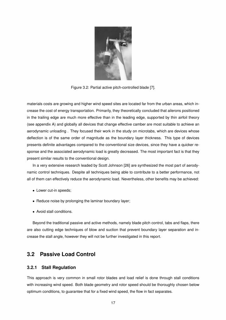
Figure 3.2: Partial active pitch-controlled blade [7].
materials costs are growing and higher wind speed sites are located far from the urban areas, which in-
crease the cost of energy transportation. Primarily, they theoretically concluded that ailerons positioned
in the trailing edge are much more effective than in the leading edge, supported by thin airfoil theory
(see appendix A) and globally all devices that change effective camber are most suitable to achieve an
aerodynamic unloading . They focused their work in the study on microtabs, which are devices whose
deflection is of the same order of magnitude as the boundary layer thickness. This type of devices
presents definite advantages compared to the conventional size devices, since they have a quicker re-
sponse and the associated aerodynamic load is greatly decreased. The most important fact is that they
present similar results to the conventional design.
In a very extensive research leaded by Scott Johnson [26] are synthesized the most part of aerody-
namic control techniques. Despite all techniques being able to contribute to a better performance, not
all of them can effectively reduce the aerodynamic load. Nevertheless, other benefits may be achieved:
• Lower cut-in speeds;
• Reduce noise by prolonging the laminar boundary layer;
• Avoid stall conditions.
Beyond the traditional passive and active methods, namely blade pitch control, tabs and flaps, there
are also cutting edge techniques of blow and suction that prevent boundary layer separation and in-
crease the stall angle, however they will not be further investigated in this report.
3.2 Passive Load Control
3.2.1 Stall Regulation
This approach is very common in small rotor blades and load relief is done through stall conditions
with increasing wind speed. Both blade geometry and rotor speed should be thoroughly chosen below
optimum conditions, to guarantee that for a fixed wind speed, the flow in fact separates.
17

Passive approach is privileged over active control, since it provides an effective blade unloading with-
out any additional moving parts, contrasting with what happens in active control. The obvious conclusion
is that is possible to achieve significant savings in weight. Additionally, all active control systems require
further attention in maintenance, because they are rather more susceptible to fail than a passive control
blade design [10]. Hence, these two factors give a definitive contribution to a lower cost of energy with
lower cost of manufacturing [29], [30].
However, this approach presents unpleasant issues in starting situations, that can only be overcome
by using higher rotor torques. Furthermore, passive techniques do not respond to local variations,
whereas active load approach can independently adapt to each blade and be more beneficial to the
rotor performance [27].
3.2.2 Aerolastic Tailoring
For a long time wind turbine blades have been built with composite materials, which brings a new set of
opportunities regarding the anisotropic properties of those materials. Even so, the research in this field
is not sufficiently developed, specially what regards simulation tools [31].
The baseline idea of aeroelastic tailoring is to take advantage of the blade twist and passively adapt it
to the incident wind loading. Goeij [10] gave an elegant definition of aeroelastic tailoring in his work: ”the
incorporation of directional stiffness into a structural design to control aerolastic deformation, whether
static or dynamic, in such a fashion as to affect the aerodynamic and structural performances of that
structure in a beneficial way”. This design is quite interesting, since it may provide lower fatigue loads
with changes in angle of attack due to sudden wind gusts. Moreover, the angle of attack may be adjusted
to each wind speed to obtain an optimal torque.
3.2.3 Bend-Twist Coupling
At the end of the last century, Goeij and his colleagues [10] studied, for various box beam configurations,
the implementation of bend-twist coupling (BTC) on the blade to reduce the maximum loads. The initial
assumptions behind their work is that the blade deforms as a reaction to the wind incidence, so it both
bends (pure bending) and twists around the rotor axis. It can twist either in the direction of stall, meaning
that there is an increase in the angle of attack, or towards feather, representing a decrease in the angle
of attack. It was concluded that conventional designs with single spar box beams present problems
when the fibre orientation is unidirectional, and the authors suggest adding different orientations to
increase the fatigue resistance. A double spar box beam design is presented. The induced twist of
this configuration is necessarily lower than a conventional design, although the objective maximum load
reduction may still be valid.
BTC can be obtained with a base design that includes sweep along the blade. This design creates
a moment that induces twist on the blade. Another possible solution is to deviate the composite fibres
away from the principal axis sufficiently to generate twist motion and decrease the load applied, taking
advantage from the non-isotropic properties of composite materials.
18

Figure 3.3: Comparison of a) conventional blade; b) bending-twist coupled blade [10].
A very recent study [5], working under the latter assumption, investigated different methods to obtain
bend-twist coupled blades. The initial assumption is that this aeroelastic behaviour can be achieved with
an unbalanced symmetrical stack of composite layers. The results obtained show that more unbalanced
stacks cause higher levels of BTC. The BTC can be quantified from the simplified reduced cross section
stiffness matrix [32],
EI −S
−S GJ
kbkt
=
Mb
Mt
, (3.1)
where EI and GJ are bending and torsional stiffness, respectively, kb is the bending curvature, kt is the
rate of twist, Mb and Mt are bending and torsional moment, respectively and S is the coupling stiffness.
The normalized BTC coefficient β can be estimated by:
β =−S√EI ·GJ
0 < β < 1. (3.2)
In the case of S = 0, the structure show the conventional response, given by
kb =M
EI. (3.3)
The BTC can be modified by changing laminate properties, in such a way that the stack becomes
unbalanced. This can be done, either by changing the layer orientation, its thickness, or by further
19

changing the materials. The results show that BTC is improved when combining the three methods
above, it means that BTC is proportional to the amount of unbalance applied on composite laminate
[24].
Ashvill [33] states that bend-twist coupling can reduce fatigue and limit operating loads. He also
concludes that the potential improvement is quite attractive, namely on the structural properties that can
be obtained. Nevertheless, further technological improvements, such as CFD and 3D validation tools,
should be achieved to justify this design manufacturing.
The comparison between stalled and feathered regulated wind turbine blades with bend-torsion cou-
pling were also investigated [34]. For both cases, the elastic strains are greater than usual and eventually
exceed the elastic limit of composite material. Twist towards feather continuously increases the turbine
output power and may conduct to unstable phenomena. Twist towards stall increases the output until
close to the rated value and then starts a negative trend. However, the output power above the rated
wind speed may compromise the economic viability of this passive control.
BTC design in fixed-speed and variable speed rotors was explored, resulting in an equivalent power
production to the uncoupled blades and significant reductions in fatigue loads. However this kind of
study should be followed by aeroelastic stability studies in order to identify the limits of stable operation
[25].
20

,
21

Chapter 4
Aerodynamic Model
4.1 Incompressible Potential Flow Fundamentals
This kind of flow is also known as irrotational flow, essentially because is assumed that the fluid particles
do not rotate or distort, therefore the vorticty is zero. For this reason, the flow is also inviscid, as viscous
effects are deeply related with the rotation of fluid particles. Figure 4.1 exemplifies an irrotational flow,
where the local reference axis does not rotate in relation to a global reference frame.
Figure 4.1: Circulation [11].
It can be demonstrated that in a velocity field, the velocity is equal to the vorticity [12]:
η = ∇× V (4.1)
Thus, two situation may occur:
• ∇ × V 6= 0: at every point in a flow leads to a rotational flow. The fluid elements have a finite
angular velocity;
• ∇ × V = 0: at every point in a flow leads to a irrotational flow. The fluid elements move in pure
translation.
The total amount of vorticity in any plane region within a flow field is called circulation, Γ. This quantity
can be seen as the vorticity flux in a region A, expressed as:
Γ =
∫ ∫A
∇× V dA ≡∮C
V · ds. (4.2)
22

Thus, circulation is equal to the integration in a line segment ds around a closed curve C (illustrated
in figure 4.22 ) in the flow, whose an arbitrary point has a velocity V . Despite the lack of prediction of
viscous effects on a real flow, potential flow is still extremely useful to study slender bodies at low angles
of attack with attached boundary layers until the trailing edge. These conditions should be guaranteed
in order to achieve accurate results, otherwise low a pressure wake is formed and the friction drag
component greatly increases, which is not predicted by potential flow.
Figure 4.2: Schematic representation of a vortex [11].
From the reasoning already made, it is clear that not only drag depends on the viscous effects, but
also lift only exists if viscosity is not neglected, since that is the condition to vorticity being different from
zero, and therefore the presence of circulation. Thus, how to calculate lift in a inviscid flow? The Kutta
Condition is the solution to that apparent paradox, and states that the flow should leave the trailing edge
smoothly, so the velocity should be finite. That is ensured placing one or more vortices with such a
strength that generates enough circulation to satisfy Kutta condition.
Recalling equation (4.1) for an irrotational flow, and considering a scalar function φ, then
∇× (∇φ) = 0 (4.3)
the curl of the gradient of that function is equal to zero. From equations (4.1) and (4.3), yields
v = ∇φ, (4.4)
which states that, for an irrotational flow, there exists a scalar function φ, with a velocity given by the
gradient of φ
Futhermore, in an imcompressble flow, the time rate of change of volume of a fluid element per unit
volume is zero, since in such flow the volume is constant, yielding:
∇ · V = 0. (4.5)
Combining equations (4.4) and (4.5)
∇ · (∇φ) = 0 (4.6)
is possible to get a very familiar equation:
23

∇2φ = 0, (4.7)
known as the Laplace’s equation.
For an incompressible flow also exists a function ψ(x, y) = constant, denoted by streamline. In
cartesian coordinates:
u =∂ψ
∂y(4.8)
v = −∂ψ∂x
(4.9)
It also can be demonstrated that equation (4.7) can also be satisfied for stream function [12]:
∂2ψ
dx2+∂2ψ
∂y2= 0. (4.10)
The demonstration assumes that any irrotational and incompressible flow have both potential and
stream function in two dimensional flow that both satisfy Laplace’s equation. Conversely, any solution
of Laplace’s equation represents the velocity potential or stream function for any irrotational and in-
compressible flow. The Laplace’s equation is linear, second-partial differential equation, therefore any
solution of linear differential equation is also a solution of the equation.
4.1.1 Boundary Conditions
Far away from the body it is assumed that velocity is alligned with x-axis, as shown in figure 4.3, therefore
it has only one component non-zero:
u = U, (4.11)
v = 0. (4.12)
Figure 4.3: Infinity and wall boundary conditions [12].
Moreover, the fluid cannot penetrate the body; the velocity it has only tangential component on the
surface, yielding
24

(∇φ) · n = 0, (4.13)
where n is a unitary normal vector of the surface. This leads to the conclusion that the body surface
itself is a flow streamline.
4.1.2 Vortex Flow
There are several possible flow fields to model a steady flow, however only the two-dimensional vortex
will be explained with more detail, because it is part of the aerodynamic model developed. This flow can
be seen as a chain of rotating particles spinning around a common axis. Potential and stream function
φ and Φ respectively, are defined as
φ =Γ
2πθ (4.14)
Ψ = − Γ
2πlnr (4.15)
The flow has a singularity when r = 0, however in real situations, the viscous effects would prevent
the flow velocity going to infinity and induce the flow to rotate as a solid body. The velocity only has a
tangential component and the streamlines are concentric circles, as show in figure 4.4 depending only
on the circulation, that measures the velocity of the flow around the origin.
Figure 4.4: Vortex [11].
4.1.3 Actuator Disk Concept
This model was initially very useful in the beginning of last century, in the calculation of performance pa-
rameters about ship propellers. In wind energy field is frequently applied to determine limits of operation
of wind turbine rotors [9]. In this mathematical concept a control volume is defined, whose boundaries
are two cross section and the surface of stream flow. The rotor is represented by an ”actuator disk”
like figure 4.5 , that creates a discontinuity of pressure in the stream flow that is crossing it. Several
assumptions are done to perform this analysis [14]:
• Homogeneous, incompressible, steady state flow;
• No friction drag;
25

Figure 4.5: Schematic representation of 1-D wind turbine blade [9].
• Uniform thrust over rotor area;
• Static pressure far upstream and downstream of the rotor equals the ambient static pressure;
Applying the momentum conservation equation on the control volume, one can relate the total thrust
with upstream and downstream velocities as
T = U1(ρAU)1 − U4(ρAU)4 = m(U1 − U4), (4.16)
where ρ is the air density, A the cross sectional area, Ui the air velocity and m the mass flow rate.
Thrust can also be expressed from the pressure difference in the actuator:
T = A2(p2 − p3) =1
2ρA2(U2
1 − U24 ). (4.17)
Reminding that m = ρA2U2, it is possible to infer about velocity across the disk,
U2 =U1 + U4
2. (4.18)
Hence, in this simple model, the velocity in rotor plane is the average of upstream and downstream
velocity.
The fractional decrease in wind speed velocity between upstream and rotor plane is called axial
induction factor, and is given by
a =U1 − U2
U1. (4.19)
In a rotating wind turbine rotor, the torque imposed to the flow, induces a rotation in the opposite
direction, as a reaction to the force exerted.
The rotational kinetic energy, represented in 4.6, influences negatively the total energy production
and, in general, wind turbines with high torques experience more rotational kinetic energy. In this case,
it is convenient to define another quantity, known as angular induction factor,
a′ =ω
2Ω, (4.20)
26
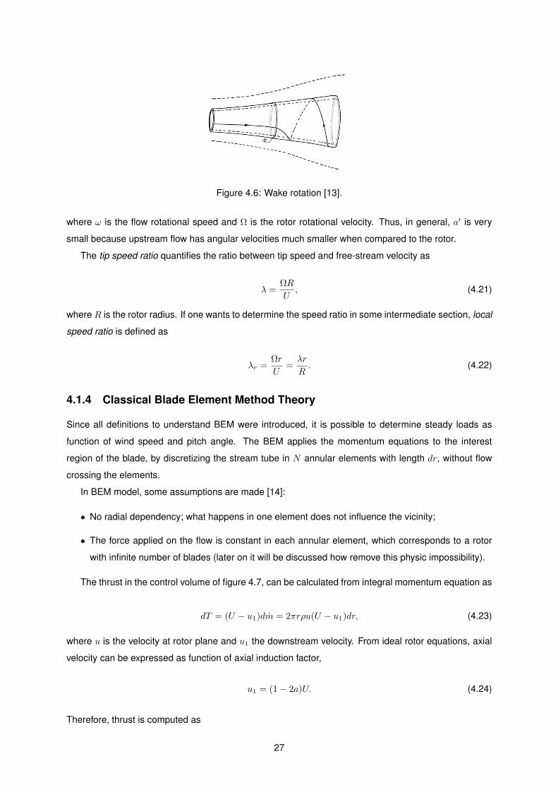
Figure 4.6: Wake rotation [13].
where ω is the flow rotational speed and Ω is the rotor rotational velocity. Thus, in general, a′ is very
small because upstream flow has angular velocities much smaller when compared to the rotor.
The tip speed ratio quantifies the ratio between tip speed and free-stream velocity as
λ =ΩR
U, (4.21)
where R is the rotor radius. If one wants to determine the speed ratio in some intermediate section, local
speed ratio is defined as
λr =Ωr
U=λr
R. (4.22)
4.1.4 Classical Blade Element Method Theory
Since all definitions to understand BEM were introduced, it is possible to determine steady loads as
function of wind speed and pitch angle. The BEM applies the momentum equations to the interest
region of the blade, by discretizing the stream tube in N annular elements with length dr, without flow
crossing the elements.
In BEM model, some assumptions are made [14]:
• No radial dependency; what happens in one element does not influence the vicinity;
• The force applied on the flow is constant in each annular element, which corresponds to a rotor
with infinite number of blades (later on it will be discussed how remove this physic impossibility).
The thrust in the control volume of figure 4.7, can be calculated from integral momentum equation as
dT = (U − u1)dm = 2πrρu(U − u1)dr, (4.23)
where u is the velocity at rotor plane and u1 the downstream velocity. From ideal rotor equations, axial
velocity can be expressed as function of axial induction factor,
u1 = (1− 2a)U. (4.24)
Therefore, thrust is computed as
27

Figure 4.7: Domain control volume [14].
dT = 4πrρU2a(1− a)dr. (4.25)
The velocity component Vrel in an annular section, is the vectorial combination between tangential
and axial velocity in that element. Figure 4.8 makes a schecmatic representation of all velocity compo-
nents and their decomposition.
Figure 4.8: Schematic represetation of aerodynamic angles [14].
θ is the blade local pitch angle, which is the sum of design pitch angle, θ0 and local twist angle, β. The
former is measured between tip chord and rotor plane and the latter is measured relative to tip chord.
φ is the angle between the plane of rotation and relative velocity, Vrel. Thus, the local angle of attack is
defined as
α = φ− θ. (4.26)
From trigonometric properties, φ is given by:
tanφ =(1− a)V0(1 + a′)ωr
. (4.27)
Maintaining the same notation, then V0 = U . It is also necessary to define σ, solidity, which is fraction
of the control volume covered by the blades:
σ(r) =c(r)B
2πr, (4.28)
where B is the number of blades, c(r) is the local chord and r is radial position. From now on, B = 1.
28

4.2 Numerical Models
4.2.1 Panel Method
This well known method, was very popular among the scientific community in the 1970s, since it allows
the calculation of aerodynamic properties of bodies with different shapes, thickness and orientation [12].
The main idea behind panel method is to cover the body of a vortex sheet and wrap it, as it may work as
streamline of the flow [11]. A schematic representation of 2D panel method is shown in figure 4.9.
The body surface is divided in n panels, where for each one exists a vortex of strength γj , usually
dimensionalised by a length unit, and has an unknown value.
Figure 4.9: Surface discretization by panels [12].
An arbitrary point P located at a (x, y) position has an induced potential velocity due to the influence
of a jth panel is given by:
φj = − 1
2π
∫j
θpjγjdsj , (4.29)
where θpj is the angle in relation to x axis of rpj , that is the distance between point P and jth panel.
θpj = atan
(y − yjx− xj
). (4.30)
The influence of all panels in potential velocity at point P is the summation of equation (4.29) over all
panels:
φ(p) =
n∑j=1
φj . (4.31)
At the control points, which are in the mean position of a panel, the normal velocity is zero. This
velocity is the superposition of uniform flow velocity and the induced velocity by all vortex panels. The
normal component of Un in the ith panel is given by
Un = Uncosβi. (4.32)
29

The normal component of induced velocity at point a (xi, yi) position on the vortex panel is given by
Vn,i =∂
∂ni[φ(xi, yi)] = −
n∑j=1
γj2π
∫j
∂θi,j∂ni
dsj . (4.33)
However, the boundary condition states that the summation of the components of velocity must be
zero, yielding
Un + Vn = 0⇔ V∞cosβi −n∑j=1
γj2π
∫j
∂θi,j∂ni
dsj = 0. (4.34)
Equation(4.34) generates a linear algebraic system of equations in order to determine n unknowns
γ1, ..., γn. In figure 4.10, the Kutta condition must be satisfied. This can be done in a couple different
ways. The easiest solution is just equal the velocities in the points that form the trailing edge, but for
an accurate solution, the gap between should be relatively close [19]. Therefore, one more equation is
added to the system of equations, yielding
γj = −γj−1. (4.35)
Therefore, the total number of equation is now n + 1 for n unknowns. One equation should vanish
and be replaced by equation (4.35), so one control point is ignored to turn the linear system possible to
solve.
Figure 4.10: Numerical incompatibility in trailing edge [12].
Another possible solution would be the extrapolation of velocities from upper and lower surface to
estimate the trailing edge velocity [19].
4.2.2 BEM Iterative Solution
This section is fundamental to understand how aerodynamic interaction affects the structure, since with
BEM is possible to estimate the steady load applied on the structure, by implementing the iterative
procedure that will be presented.
As any iterative solution, it is necessary to guess some initial values. In this case, both axial and
angular induction factor, a and a′ respectively, will be set to zero. Another possible guess would be using
equations of optimum blade design [9], that will not be presented.
As shown in equation (4.36), the angle φ depends on a and a′:
30

tanφk =U(1− ak)
Ωr(1 + a′k)=
1− ak(1 + a′k)λr
, (4.36)
where k is kth iteration.
It is usual apply the Prantl’s tip correction factor [13] in order to take into account the pressure loss
on that region:
Fk =
(2
π
)cos−1
[exp
(− (1/2)[1− (r/R)]
(r/R)sinφk
)]. (4.37)
Other corrections can be introduced, such as Gluaert’s correction, which applies an adjustment in
momentum equation due to discrepancies in torque coefficent in case of high axial induction factors,
tipically grater than 0.4, where the wake is predominantly turbulent [35]:
CTk=
8
9+
(4Fk +
40
9
)+
(50
90− 4Fk
)a2k. (4.38)
One more correction is frequently applied to the lift coefficient at inner sections of the blade. In that
region, the centrifugal forces are especially strong and boundary layer thickness is significantly reduced,
thereby delaying the separation phenomena [35]. Thus, the correction in lift coefficient yields:
CL3D= CL3D
+3.1λ
1 + λ2g( cr
)2 [(dCL2D
dα
)linear
sin(ak − a1)− CL2D
], (4.39)
where g is the blending factor that guarantees a smooth geometrical transition of polar curves.
According to equation 4.26, the local angle of attack is computed as follows:
αk = φk − θTk. (4.40)
From airfoil data, is possible to extract an interpolated Cl value and conclude the iterative process
updating new values for axial and angular induction factors, closing the loop with the following expres-
sions:
ak+1 =1
1 + 4Fksin2(φk)σClkcosφk
, (4.41)
a′k+1 =1
4Fkcos(φk)σClk
− 1. (4.42)
This set of routines should be executed until a prescribed convergence criterion is reached. Then, it
is possible to access the corresponding Cp data regarding the converged angle of attack.
In the fluxogram of figure 4.11, it is possible to have a general overview about the set and sequence
of routines usually applied in any BEM code.
31

Guess a and a′
Calculate φ
Calculate α
CL interpolation
Computationof correc-
tion factors
a and a′b haveconverged?
Update ai =a(Cli−1) anda′i = a′(Cli−1)
Load com-putation
no
yes
Figure 4.11: Fluxogram about BEM iterative solution.
4.3 Description of Aerodynamic Routine Program aero load.m
4.3.1 Purpose and Objectives
During the course of this work, it became of particular interest automate the aerodynamic force com-
putation regarding a fixed wind speed, therefore was developed a numerical tool in the commercial tool
MATLAB R©. The algorithm obtains a pressure distribution in a blade surface, following the principles
of panel method and BEM, that were briefly revisited in sections 4.2.1 and 4.2.2.
4.3.2 Input Variables
The code receives previously the mesh computed by structural model, and additionally needs an esti-
mated value for λ .
32

4.3.3 Pressure distribution
From the input variables, the algorithm developed runs in the background an auxiliary software XFoil.
This tool applies a 2-D panel method, in inviscid and incompressible flow conditions [36],[37]. It is open
source, that is why it is very common in early design tests, since provides satisfactory results with very
low computational effort. The software receives input variables regarding flow conditions, such as free-
stream wind speed, air density, Reynolds number and Mach Number. Additionally, the airfoil section
coordinates are necessary in order to perform an aerodynamic analysis. The airfoil can be created
either by XFoil NACA airfoil generator, or from an output file containing the (x, y) coordinates of the
aiorfoil. Whenever the latter option is chosen, it is necessary to pay special attention to the trailing edge
coordinate. The two nearest points of trailing edge should be sufficiently distant in order to XFoil itself,
apply the boundary conditions to meet Kutta condition. Then, the software executes the analysis and
save the Cp output files, one per angle of attack. Once the blade operational angle of attack is initially
unknown, this range should be sufficiently large to include the converged value obtained by BEM later
on.
At the root section, it was created an exception in the Cp calculation due to numerical problems
in XFoil. This region does not have an aerodynamic shape and XFoil does not converge the solution
for a large number of angles of attack. Nevertheless, another simplistic solution was adopted. It was
assumed that this region only contains circular sections and applying the potential flow theory, it is
possible to demonstrate that for any circular section, the Cp distribution is given by [38]
Cpr,j = 1− 4sin2θTr , (4.43)
where the subscript r represent the blade radial position and j is the jth panel. Since XFoil is limited to
2-D Cp distributions, the Cp for all blade surface was estimated through bi-linear interpolations.
4.3.4 BEM Computation
The implementation of BEM is followed step by step as presented in section 4.2.2, so a and a′ are set
to 0 in the first iteration. The relative angle φ, depends on the tip speed ratio, λ, which depends on
the blade geometry and is usually available in WT catalogues. The BEM iterative method reaches a
converged solution very quickly due to the simplicity of the equations. Trials demonstrated that, typically,
with less than six iterations is possible to reach a converged solution.
Recalling equation (4.40), it is important explain in detail the components of θTr. The total pitch has
three origins:
θTr= θ0r + θa.c.r + βr, (4.44)
where θ0i is the designed twist angle and section property, so its value remains always constant; θa.c.i
is the active control pitch angle. It also remains constant during all iterations but should be set in
the beginning of the simulation. This term might be useful to have an insight about coupling between
33

passive and active control systems; βi is the twist of structural reaction. In each solution of BEM, θi
remains constant, however later on when this model is combined with the structural model, in a coupled
iteration, where both aerodynamic and structural models are working, βi will change, due to surface
deformation.
The converged value of angle of attack allows the access of the Cp database created by XFoil, and
pressure distribution may be addressed to all blade surface. It should be noted that in case of two or
more different airfoils are used in the blade geometry, the same number of independent BEM calculations
are done, and, consequently, the number of operational angles of attack is equal to number of airfoils
loaded. Since the span is discretized in a large number of sections, in a region where the same airfoil
is applied (regardless of the maximum chord), an interpolation between two BEM solutions is performed
to compute the remaining values of angle angle of attack.
4.4 Aerodynamic Load Computation
The aerodynamic load is directly obtained from the pressure distribution. The non-dimensional parame-
ter of this quantity in the jth panel is given by:
Cpr,j =pr,j − p0
12ρU
2(4.45)
where the pj is the pressure in the jth panel of a radial position r, p0 is the atmospheric pressure. The
pressure due to the fluid-interaction is given by dropping p0, thus yielding:
pj = Cpj1
2ρU2. (4.46)
34

4.4.1 Program Routine
In the next fluxogram is given a global insight about the set of routines implemented in the code devel-
oped by the author.
Inputs
BEM
BEM solutionhave
converged?
Cp interpolationXFOIL
Pressurecomputation
Output- elemental Pressure
Cp database
α
no
Figure 4.12: Fluxogram about aerodynamic model framework.
35

36

Chapter 5
Structural Model
5.1 Linear Elasticity Foundations
Any body subjected to a force and temperature field experiences a displacement field [39]. Applied
loads, boundary conditions, temperature field and material stress law are necessary to determine a
body displacement field. Corresponding stress and strains are interesting quantities to determine.
The x, y, z displacements can be computed is a displacement vector u, yielding
u = u v w. (5.1)
The strain vector can have up to six independent components:
ε = εx εy εz γxy γyz γzx. (5.2)
Thus, assuming small displacements, the strain vector ε can be determined directly from the dis-
placement vector as
ε = [D]u, (5.3)
where [D] is the matrix differentiation operator given by [39]
[Di] =
∂/∂x 0 0
0 ∂/∂y 0
0 0 ∂/∂z
∂/∂y ∂/∂x 0
0 ∂/∂z ∂/∂y 0
∂/∂z 0 ∂/∂x
. (5.4)
Similarly, the stress vector σ has six diffferent components:
σ = σx σy σz τxy τyz τzx. (5.5)
37

From the Linear Elastic Theory results the Hook’s Law [39], which relates simultaneously stress and
strain components as
σ = [E](ε − εt), (5.6)
with
εt = δT δT δT 0 0 0, (5.7)
where εt represents the part of strain due to temperature, δ is the coefficient of thermal expansion, T
is the temperature. The term ε − εt includes the elastic component of strain only. [E] is the elastic
matrix,
[E] =
λ+ 2µ ξ ξ 0 0 0
ξ ξ + 2µ ξ 0 0 0
ξ ξ ξ + 2µ 0 0 0
0 0 0 µ 0 0
0 0 0 0 µ 0
0 0 0 0 0 µ
, (5.8)
where ξ and µ are constants depending on the elastic modulus E and the poisson ratio ν, given respec-
tively by
λ =νE
(1 + ν)(1− 2ν)(5.9)
and
µ =E
2(1 + ν). (5.10)
5.2 Finite Element Matrix Formulation
The structural model implemented follows the linear finite element formulation applied to 4-node shell
elements. They have six degrees of freedom per node, three translations and three rotations. This kind
of element support a very large range of strain and rotation, dealing with linear and non-linear problems.
Is also possible to model composite shells and sandwich forms, governed by first shear deformation
[16].
Considering an arbitrary three dimensional nodal displacement vector,
q = u1 v1 w1 u2 v2 w2..., (5.11)
the finite element displacement is found by
u = [N ]q (5.12)
38

Figure 5.1: 4-nodded shell element [15]..
where [N ] is the matrix that contains functions of form. The strains can also be obtained directly by
ε = [B]q, (5.13)
where [B] is called the displacement differentiation matrix and is expressed as
[Bi] =
∂Ni/∂x 0 0
0 ∂Ni/∂y 0
0 0 ∂Ni/∂z
∂Ni/∂y ∂Ni/∂x 0
0 ∂Ni/∂z ∂Ni/∂y 0
∂Ni/∂z 0 ∂Ni/∂x
. (5.14)
The solution of finite elements seek to find the minimum total potencial energy Π [39]
Π =∂
∂q
(∫V
1
2εeT σdv −
∫V
uT pV dV −∫S
uT pSdS)
(5.15)
Computing the strains and stress relations and substituting in equation (5.15) yields
Π =
(∫V
1
2
([B]q − εt
)T[E]([B]q − εt
)dV −
∫V
([N ]qT
)pV dV −
∫S
([N ]qT
)pSdS
)(5.16)
The differentiation relative to nodal displacement q, yields
∫V
[B]T [E][B]dV q −∫V
[B][E]εtdV −∫V
[N ]T pV ∫S
[N ]T pSdS = 0 (5.17)
Each integral has a significant meaning:
39

[k] =
∫V
[B]T [E][B]dV q (5.18)
p =
∫V
[B][E]εtdV +
∫S
[N ]T pSdS (5.19)
h =
∫V
[N ]T pV = 0 (5.20)
Where [k] is called the element stifness matrix, f is the load vector and h is the thermal vector,
modelling forces originated by thermal expansion.
Usually, for one element it is applied the following notation:
[k]q = f, (5.21)
f = p+ h. (5.22)
Once obtained all element equations, it is necessary to assemble them in one single system of
equations to reach the final solution. Therefore, the global system of equations is
[KG]QG = FG, (5.23)
and the total minimum potential energy is simply the sum of element potential energies:
ΠG =
num. elem∑i=1
Πi. (5.24)
5.3 Composite materials
Composite materials combine two or more materials on a macroscopic scale to achieve better properties
than the conventional materials, for instance, stiffness, strength, weight reduction, corrosion resistance,
thermal properties and fatigue life [16]. Most part of composite materials are made from two materials:
a reinforcement material called fibre and a base material, called matrix. There are various types of
composites materials, but one is interested in one in special: laminated composites. They are made
of layers of different material, and the fibres and matrix can be either metallic or non-metallic [16]. A
ply is a typical sheet of composite material. A laminate is a set of plies, stacked to achieve the desired
stiffness and thickness. For example, unidirectional plies can be stacked, so that the fibres in each
ply are oriented in the same or different directions, as shown in figure 5.2. The sequence of several
orientations of a composite layer in a laminate is known as stacking sequence.
The micromechanics field developed a set of equations that allow the determination of the elastic
constants of a composite material, assuming [16]:
• Perfect bonding between fibres and matrix;
• Fibres are parallel, and uniformly distributed;
40

• The matrix is free of voids or micro-cracks, and initially is in a stress-free state;
• Both fibres and matrix are isotropic and obey Hooke’s law;
• The applied loads are either parallel or perpendicular to the fibre direction
Figure 5.2: A stack with various unidirectional layers [16].
The constants of a lamina are given by
E11 = EfVf + Em(1− Vf ), (5.25)
E22 =EfEm
Ef (1− V f) + EmVf, (5.26)
ν12 = νfVf + νm(1− Vf ), (5.27)
G12 =GfGm
Gf (1− Vf ) +GmVf(5.28)
where E11 is the longitudinal modulus, E22 is the transversal modulus Ef is the fibre modulus, Em is
the matrix modulus, Vf and is the fibre volume fraction, νm is the matrix Poisson’s ratio, νf is the fibre
Poisson’s ratio, ν12 is the major Poisson’s ratio and G12 is the shear modulus. Matrix and fibre shear
modulus, Gm and Gf , respectively, are given by
Gm =Em
2(1 + νm), (5.29)
Gf = Ef2(1− νf ). (5.30)
5.4 Description of Structural Mesh Generator WTB struct model.m
5.4.1 Purposes and Objectives
The numerical code developed in MATLAB R© builds from a set of inputs defined by the user, a struc-
tured 1 mesh of a wind turbine blade. An output file with APDL code is created and computed in the1The elements of a structured mesh can be all indexed by three index variables i, j, k, whereas in an unstructured mesh, the
connectivity between the elements is not express in such simple manner. The connectivity between elements must be explicitlystored, therefore usually the storage requirements and computation times are more demanding [40].
41

FEM tool ANSY S R© that performs a static simulation and gives an insight about the structural response
of the structure.
5.4.2 Input Variables
The initial inputs necessary to compute the mesh are the number of divisions of blade chord, span and
webs. Additionally, the user may change the web position (in percentage of chord). Furthermore, all
coordinates concerning airfoil sections should be computed in percentage of chord and located in a .txt
file.
5.4.3 Nodes Assembly
The first action taken by MATLAB R© is compute the blade sections. The code reads the airfoil coordi-
nate files and draws them like is illustrated in figure 5.3.
Figure 5.3: Airfoil section computation.
The amount of data collected to build the blade geometry assumes a special relevance, namely
about the number of airfoil sections collected to build it. The accuracy in the interpolation is improved
if more sections are loaded previously, otherwise trailing edge position can suffer significant deviations.
Identically, it is also important to have a sufficiently large number of points in each section, as that may
affect negatively the interpolation of intermediate chord coordinates.
Nevertheless, the user has the freedom to choose the number of divisions in chord, span and webs,
then from the set of computed airfoil sections, all nodes are generated by linear interpolations of two
neighbour sections. A blade nodal representation is illustrated in figure 5.4.
42
Figure 5.4: Mesh example.
5.4.4 Elements Assembly
Following the nodes data, ANSY S R© needs to know which are the nodes that form each finite element.
Therefore, a routine to assemble all the elements was developed. The element chosen was SHELL181,
that is the one most suitable to shell structures [15]. It is constituted by four nodes, so starting in the
leading edge of root section in suction side, a sweep is done towards trailing edge to compute a line of
elements:
e(k)1 = mesh(i, j), (5.31)
e(k)2 = mesh(i+ 1, j), (5.32)
e(k)3 = mesh(i+ 1, j + 1), (5.33)
e(k)4 = mesh(i+ 1, j + 1), (5.34)
where an element k is computed by the four nodes (e1, e2, e3, e4) in the vicinity, in the anti-clockwise
direction. The direction in which the nodes are computed is not arbitrary, since the unitary normal
vector in ANSY S R© follows the right hand rule, this way the routine implemented guarantees that it is
always pointing toward the posite Y-axis. That fact is determinant to apply surface loads, once a positive
pressure load is applied in the opposite direction of the element unitary normal vector. Furthermore,
in case of using composite materials, the stack sequence is oriented according the orientation of this
vector. As soon as the sweep towards trailing edge is done, an increment in span coordinate is done
and the same routine is applied two times the number of span divisions defined by the user. The total
43

number of elements covering the blade surface is then, two times the product between the divisions in
chord and span. The same set of routines is applied to compute the webs elements.
(a) Blade surface. [7] (b) Shear webs. structure
Figure 5.5: Assembled elements.
5.5 Load and Nodal Constraints Computation
It was considered that blade is fully constrained in its root, therefore no nodal displacements nor rotations
are allowed there. The load is computed in each element surface from an APDL code computed by
MATLAB R© (see full APDL code in appendix B.1), then ANSY S R© calculate the respective force to
apply in each mesh node.
44

Chapter 6
Fluid-Structure Interaction
Until now, aerodynamic and structural analyses have being treated separately. These two distinct fields
have different domains, however, they share boundaries and, in fact, a well defined region exists where
the information between both domains can be exchanged. In that region, a three-dimensional surface,
a structural-field interface is defined [41]. On one side, the structural mesh undergoes a displacement
field, that constantly induces changes in the fluid domain, since by definition this fluid must occupy all
space available and fulfil all gaps that might exist due to deformations of the structural mesh. On the
other side, the fluid mesh is sensitive to variations in fluid stress, namely due to pressure and shear, that
will transmit through the interaction surface by means of external load to the structural domain. Thus, a
clear reciprocity is made here, and it makes all sense to couple both models and study the simultaneous
aerodynamic and structural response, as schematically shown in figure 6.1.
Figure 6.1: Exchange domain between aerodynamic and structural models.
The main concern about this topic lies on the correct definition of both mesh boundaries, since it is not
feasible in many situations to represent accordingly the interaction surface. In these cases, questionable
situations appear and it is the competence of the engineer to make the coupled system work properly
and understand ambiguous situations to maintain a valid transfer between displacement and forces.
6.1 Fluid Structure Interaction Methods
In the technical literature three major techniques of fluid-structure interaction (FSI) are presented, where
the main differences lie the on sequence to solve both aerodynamic and structural models. The compu-
tational most demanding technique is the fully coupled method, where both aerodynamic and structural
45
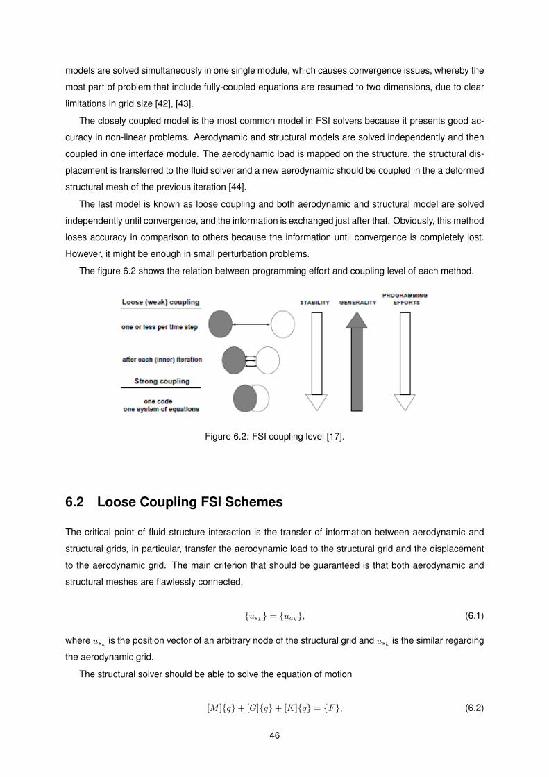
models are solved simultaneously in one single module, which causes convergence issues, whereby the
most part of problem that include fully-coupled equations are resumed to two dimensions, due to clear
limitations in grid size [42], [43].
The closely coupled model is the most common model in FSI solvers because it presents good ac-
curacy in non-linear problems. Aerodynamic and structural models are solved independently and then
coupled in one interface module. The aerodynamic load is mapped on the structure, the structural dis-
placement is transferred to the fluid solver and a new aerodynamic should be coupled in the a deformed
structural mesh of the previous iteration [44].
The last model is known as loose coupling and both aerodynamic and structural model are solved
independently until convergence, and the information is exchanged just after that. Obviously, this method
loses accuracy in comparison to others because the information until convergence is completely lost.
However, it might be enough in small perturbation problems.
The figure 6.2 shows the relation between programming effort and coupling level of each method.
Figure 6.2: FSI coupling level [17].
6.2 Loose Coupling FSI Schemes
The critical point of fluid structure interaction is the transfer of information between aerodynamic and
structural grids, in particular, transfer the aerodynamic load to the structural grid and the displacement
to the aerodynamic grid. The main criterion that should be guaranteed is that both aerodynamic and
structural meshes are flawlessly connected,
usk = uak, (6.1)
where usk is the position vector of an arbitrary node of the structural grid and usk is the similar regarding
the aerodynamic grid.
The structural solver should be able to solve the equation of motion
[M ]q+ [G]q+ [K]q = F, (6.2)
46

where [M ], [G], and [K] are the mass, gyroscopic and stiffness matrices. F is the force vector and q
is the displacement vector. Under steady axial flow conditions, the blade has a constant aerodynamic
load and the equation of motion resumes to equation 5.23. Vector F contains forces from different
natures:
F = F0+ Fg+ Faero+ Fn.l. (6.3)
where F0 is the constant force, Fg is the gravitational load, Faero is the aerodynamic load and
Fn.l. is the non-linear component. Let us assume that the unique constant force is Faero, and
neglect Fn.l. and Fg. The static equilibrium is given by
[K]q = Faero, (6.4)
which has the same meaning of equation (5.21). Faero is obtained from the aerodynamic module.
Dong Ok Yu and Oh Joon Kwon [18] presented in their research two different loose coupling methods
of FSI. The first method consists on a static FSI model running in sequence the structural and aerody-
namic model, the latter on a CFD tool basis. The structural mesh is initially undeformed and the CFD
tool calculates the aerodynamic load for the undeformed structure.
Figure 6.3: Static loose coupling FSI model [18].
47

Then, the output of the CFD solver is coupled to the FEM tool, that will apply the aerodynamic load
on the deformed mesh and give a new output relatively to an updated deformed mesh, which will be
introduced again in CFD solver. The iterative process is repeated until the convergence of Faero and
displacement vector q have been verified. The computation sequence is shown in figure 6.3. The
second method is more suited to unsteady loads and time-varying response, avoiding more demanding
methods as fully-coupled ones. In the first iteration, Faero is computed by a BEM code and the
displacement field is calculated in relation to the undeformed mesh. In its turn, the CFD solver receives
the deformed mesh, and performs the aerodynamic load calculation, regarding the deformed mesh, and
returns it to the CSM solver. This time, the total aerodynamic load in the current iteration k is given by
the CFD solution and the difference between current and previous BEM solutions as
F kaero = F kCFD+ (F kBEM − F k−1BEM). (6.5)
With this method the convergence only depends on the force.
6.3 Simplified Coupling Procedure
The last step of numerical development in the scope of this research was focused on a loose coupling
FSI model. Usually these models incorporate a CFD solver to determine the aerodynamic load which
is interacting with the structure. In this work, it is exaggerated to make that statement but, even so, it
was developed a simplified aerodynamic model which can estimate the aerodynamic load. Since the
objective of this work is to observe a mitigation in load due to the bend-twist coupling (BTC), in this model
only twist is coupled, whereas in a conventional FSI coupling model, both displacements and rotations
are returned to CFD solver. Thus, the load mitigation will be achieved exclusively by the variation in
twist.
The coupling initiates with the structural model. The aerodynamic load is treated in ANSY S R© as
a pressure load on the elements, and both aerodynamic and structural meshes are coincident, as is
illustrated in figure 6.4.
Figure 6.4: Sobreposition between aerodynamic and structural grid [17].
ANSY S R© simulation consists in a steady static analysis of the structure and the nodal displacement
field is returned to MATLAB R©. From the nodal displacements is possible infer about the amount of
twist that the blade is subjected. The correct calculation of twist would be calculating β in relation to the
48

elastic axis, however it is not possible to determine precisely where it is located. Therefore this angle is
calculated taking into account the displacement of leading and trailing edges in each span coordinate:
βi = arctan
(yit.e. − yil.e.xit.e. − xil.e.
). (6.6)
where yil.e. is the y position of the leading edge, yit.e. , is the y position of the trailing edge. The same
notation is applied to xil.e. and xit.e. .
βi is the variable updated in BEM solver, which initially is set to zero and will make the aerodynamic
load change in each iteration. The updated Faero is then introduced in MATLAB R© and the iterative
process is consecutively executed until Faero converges. Theoretically, the computation times should
not be exaggerated, since non linear effects are not being considered during the simulations.
The generic coupling sequence is represented in figure 6.5 and it shows the framework of all numer-
ical models developed during the course of this work.
AerodynamicGrid Structural Grid
BEM
Load Com-putation
Structural LoadComputation
StructuralDisplacement
Convergencecriterion
satisfied?
Final Solution
No
Yes
Figure 6.5: Fluid-structure interaction iterative solution.
49

50

Chapter 7
Parametric Study
In this chapter will be introduced a baseline configuration that will serve as comparison to perform a
parametric study. It will be computed and analysed four different and independent parameters: fibres
laminate orientation, thickness distribution, shear webs number and location and material reinforcement.
The results of each study will be discussed and summarized in the end.
7.1 Wind Turbine NREL 5 MW Data
The computational model developed in the present work has been used to characterize both the aero-
dynamic and structural performance of a wind turbine blade. The blade under test is part of a quite
common wind turbine in offshore applications developed by the National Renewable Energy Laboratory,
NREL [45]. This USA entity intended to gather more knowledge to build sites in american deep waters
and worldwide. From the experience of other companies, it was concluded that a wind turbine becomes
cost-effective on an offshore application when the output power is between 5 and 20 MW. A baseline 5
MW wind turbine was chosen, since there are several publications about this conceptual design, and the
largest wind turbine prototypes in 2009 had this rating [45]. Table 7.1 presents the wind turbine baseline
properties.
The blade is constituted by a mixture of TU Delft and NACA airfoil shapes, while the root region
contains circular sections. The transition region is not clearly documented. In table 7.2 it is possible to
consult the different airfoils used in the NREL 5MW blade. It was not possible to find any data about TU
Delft airfoils, and they were replaced by identical airfoils from NACA series, as shown in table 7.3. The
location of maximum thickness and camber were maintained equal to the values used in tip airfoil.
It was collected additional geometrical data to develop the blade geometry, listed in table 7.4.
51
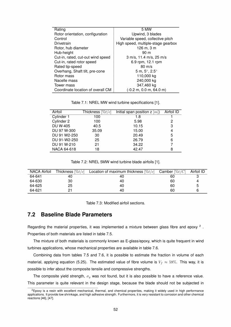
Rating 5 MWRotor orientation, configuration Upwind, 3 bladesControl Variable speed, collective pitchDrivetrain High speed, multiple-stage gearboxRotor, hub diameter 126 m, 3 mHub-height 90 mCut-in, rated, cut-out wind speed 3 m/s, 11.4 m/s, 25 m/sCut-in, rated rotor speed 6.9 rpm, 12.1 rpmRated tip-speed 80 m/sOverhang, Shaft tilt, pre-cone 5 m, 5, 2.5
Rotor mass 110,000 kgNacelle mass 240,000 kgTower mass 347,460 kgCoordinate location of overall CM (-0.2 m, 0.0 m, 64.0 m)
Table 7.1: NREL MW wind turbine specifications [1].
Airfoil Thickness [%t/c] Initial span position z [m]) Airfoil IDCylinder 1 100 1.8 1Cylinder 2 100 5.98 2DU W-405 40.5 10.15 3DU 97 W-300 35.09 15.00 4DU 91 W2-250 30 20.49 5DU 91-W2-250 25 26.79 6DU 91 W-210 21 34.22 7NACA 64-618 18 42.47 8
Table 7.2: NREL 5MW wind turbine blade airfoils [1].
NACA Airfoil Thickness [%t/c] Location of maximum thickness [%t/c] Camber [%t/C] Airfoil ID64-641 40 40 60 364-630 30 40 60 464-625 25 40 60 564-621 21 40 60 6
Table 7.3: Modified airfoil sections.
7.2 Baseline Blade Parameters
Regarding the material properties, it was implemented a mixture between glass fibre and epoxy 2 .
Properties of both materials are listed in table 7.5.
The mixture of both materials is commonly known as E-glass/epoxy, which is quite frequent in wind
turbines applications, whose mechanical properties are available in table 7.6.
Combining data from tables 7.5 and 7.6, it is possible to estimate the fraction in volume of each
material, applying equation (5.25). The estimated value of fibre volume is Vf ≈ 59%. This way, it is
possible to infer about the composite tensile and compressive strengths.
The composite yield strength, σy was not found, but it is also possible to have a reference value.
This parameter is quite relevant in the design stage, because the blade should not be subjected in
2Epoxy is a resin with excellent mechanical, thermal, and chemical properties, making it widely used in high performanceapplications. It provide low shrinkage, and high adhesive strength. Furthermore, it is very resistant to corrosion and other chemicalreactions [46], [47].
52

Span position z [m] Twist Chord Length [m] Airfoil ID2.8667 13.31 3.54 15.6 13.31 3.85 18.33 13.31 4.17 211.75 13.31 4.56 315.85 11.48 4.65 419.95 10.16 4.46 424.05 9.01 4.25 528.15 7.80 4.01 632.25 6.54 3.75 636.35 5.36 3.50 740.45 4.19 3.26 744.55 3.13 3.01 848.65 2.32 2.76 852.75 1.53 2.52 856.17 0.86 2.31 858.17 0.86 2.31 858.90 0.37 2.09 861.63 0.11 1.42 8
Table 7.4: Blade geometrical data [2].
Glass fibre EpoxyDensity ρ [Kg/m3] 2550 1110Tensile modulus E [GPa] 70 5Tensile strength σut [MPa] 3510 80Poisson ratio ν 0.2 0.4Compressive strength σuc [MPa] 910 133Yield strength σy [MPa] — 20.4
Table 7.5: Mechanical properties of fibre glass and epoxy [3], [4].
Density ρ [kg/m3] 1920Longitudinal modulus E11 [GPa] 43.2Transversal modulus E22 [GPa] 12.6Poisson coefficient ν 0.38Distortion modulus G [GPa] 4.2
Table 7.6: E-glass/Epoxy composite mechanical properties [5].
any moment to a stress near this value. The composite yield strength is the stress indexed to the
first material constituting the composite laminate, achieving plastic deformations. In general, the matrix
Young’s modulus is inferior than the fibres, thus it is the first achieving the plastic regime. Therefore, the
composite’s yield strength is given by [48]
σyc = E11σymEm≈ 176.6 MPa. (7.1)
The baseline configuration contains laminates with constant thickness, 8 layers oriented in the blade
plane, +45 degrees in relation to the edgewise axis. Figure 7.1, it is plotted the laminate stack.
The free-stream wind velocity was set to 25 m/s, equal to catalogued rotor cut-out speed, and crosses
the blades from the leading to the trailing edge, as usual. Figure 7.2 illustrates the surface load applied
53

Figure 7.1: Fibres orientation.
on the blade at the suction and pressure sides.
(a) Lower surface. (b) Upper surface.
Figure 7.2: Pressure distribution on blade surface.
The suction pressure is concentrated in the thicker airfoils region of upper surface, whereas high
pressure is distributed by all blade lower surface. In the leading edge, the stagnation points are concen-
trated, which means, velocity tends to zero and high pressure peaks are formed.
Furthermore, it was considered an initial position of shear webs at 45% and 75% of chord. The
simulations performed in the parametric study did not couple the effective blade twist due to the amount
of time that would be spent to study each parameter. At this stage, it is more important to understand
how each parameter affect the structural response and, one iteration is enough to trace this trend. A
structural mesh with a total of 4770 elements was computed, 4000 elements model the skin surface, the
remaining elements model shear webs.
54

7.3 Baseline Results
7.3.1 Structural Performance
The structural analysis shows expected trends in the results, as both edgewise and flapwise displace-
ments continuously increase towards blade tip (in absolute values). The shear webs deformation, in
figure 7.3(b) follows the same pattern of the exterior surface, in figure 7.3(a).
(a) Blade surface (b) Webs
Figure 7.3: Baseline deformation.
(a) Edgewise displacement at (x/c) = 25% (b) Flapwise displacement at (x/c) = 25%
(c) Twist distribution
Figure 7.4: Baseline displacement and twist distribution.
55

With respect to twist in figure 7.4(c), it starts a pronounced curve until 10 m, that is slightly attenuated
by the presence of shear webs since then. The general trend is increase of twist through the span, which
is exactly the opposite desired behaviour. This situation would conduct to a situation of an increase of
blade angle of attack until it gets stalled. The following section will explain more in detail this question
through two contrasting situations. The sudden change in twist reported previously, is the major source
of stress, as shown in figure 7.5, as the maximum is obtained in the same span position illustrated
by 7.4(c). An enhanced configuration should take into account an eventual overstress in this region.
Nevertheless, by now, absolute values fulfil the von Mises failure criterion (that is presented in Appendix
A.1), as confirmed in table 7.7.
Layers θ [] ymax [m] xmax [m] |βmax| [] σeqv,max [MPa]+45 2.36 −0.31 −0, 80 29.8
Table 7.7: Baseline maximum values.
(a) Suction side (b) Pressure side
(c) Webs
Figure 7.5: Baseline von Mises equivalent stress.
56
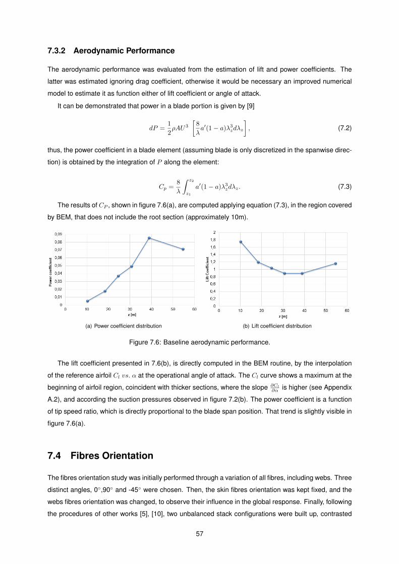
7.3.2 Aerodynamic Performance
The aerodynamic performance was evaluated from the estimation of lift and power coefficients. The
latter was estimated ignoring drag coefficient, otherwise it would be necessary an improved numerical
model to estimate it as function either of lift coefficient or angle of attack.
It can be demonstrated that power in a blade portion is given by [9]
dP =1
2ρAU3
[8
λa′(1− a)λ3zdλz
], (7.2)
thus, the power coefficient in a blade element (assuming blade is only discretized in the spanwise direc-
tion) is obtained by the integration of P along the element:
Cp =8
λ
∫ z2
z1
a′(1− a)λ3zdλz. (7.3)
The results of CP , shown in figure 7.6(a), are computed applying equation (7.3), in the region covered
by BEM, that does not include the root section (approximately 10m).
(a) Power coefficient distribution (b) Lift coefficient distribution
Figure 7.6: Baseline aerodynamic performance.
The lift coefficient presented in 7.6(b), is directly computed in the BEM routine, by the interpolation
of the reference airfoil Cl vs. α at the operational angle of attack. The Cl curve shows a maximum at the
beginning of airfoil region, coincident with thicker sections, where the slope ∂Cl
∂α is higher (see Appendix
A.2), and according the suction pressures observed in figure 7.2(b). The power coefficient is a function
of tip speed ratio, which is directly proportional to the blade span position. That trend is slightly visible in
figure 7.6(a).
7.4 Fibres Orientation
The fibres orientation study was initially performed through a variation of all fibres, including webs. Three
distinct angles, 0,90 and -45 were chosen. Then, the skin fibres orientation was kept fixed, and the
webs fibres orientation was changed, to observe their influence in the global response. Finally, following
the procedures of other works [5], [10], two unbalanced stack configurations were built up, contrasted
57

with a balanced stack. The table 7.9 describe the stack employed in multi-directional laminates.
The recorded results in figures 7.7 to 7.10, evidence in first place that, the layers orientation can
affect significantly the results, therefore the choice criterion should be thorough.
Skin θ [] Webs θ [] ymax [m] xmax [m] |βmax| [] σeqv,max [MPa]0 0 2.26 −0.30 −0.17 31.9−45 −45 2.31 −0.31 0.73 35.990 90 0.77 −0.12 −0.15 27.0
+45 0 2.36 −0.31 −0.8 30.6+45 −45 2.36 −0.31 −0.8 31.8+45 90 2.08 −0.28 −0.69 38.5
Balanced Balanced 1.08 −0.14 −0.15 38.2Unbalanced 1 Unbalanced 1 1.10 −0.15 −0.18 39.0Unbalanced 2 Unbalanced 2 1.09 −0.15 −0.14 37.6
Table 7.8: Layers orientation; maximum values.
Laminate Label Skin θ [] Webs θ []Balanced [902|25|45| − 45| − 25|902] [902|25|45| − 45| − 25|902]
Unbalanced 1 [902|25|45]S [902|25|45]SUnbalanced 2 [902| − 25| − 45]S [902| − 25| − 45]S
Table 7.9: Multi-directional Laminates stack.
Figure 7.7: Twist distribution for different fibres orientation.
The stacks with unidirectional fibres proved to be very ineffective either in the amount of deformation
caused or in the induced twist, presented in table 7.8. This table shows the maximum values, regarding
both the flapwise and edgewise displacement (not necessarily at (x/c) = 25%), twist and stress. Nev-
ertheless, it should be noted that fibres oriented -45 +45, despite the high nodal displacement, bring
great benefits in the induced twist in comparison with baseline results, but only the -45 fibres induce a
positive ∆β, i.e., a reduction in angle of attack. The definitions of β in equation (6.6), and α in equation
(4.26), state that only a positive ∆β, calculated by equation (6.6) can generate a reduction in angle of
58

attack. The response verified by the variation in webs layers orientation is not very different from the
unidirectional stack response.
The introduction of layers in different direction, yielding a multi-directional stack provided significant
savings in maximum displacement, illustrated in figures 7.9 and 7.8, but did not produce desired effect
in twist, as a negative ∆β result in an increase of the angle of attack.
Figure 7.8: Flapwise displacement at (x/c) = 25% for different fibres orientation.
Figure 7.9: Edgewise displacement at (x/c) = 25% for different fibres orientation.
The stress plots in figures 7.10 and 7.11 evidence predominantly stress peaks in the shear webs
insertion, which reinforces the importance of having these structures to provide a relevant source of
stiffness to the structure.
59

(a) von Mises equivalent stress distribution: θskin = 0,θweb = 0 .
(b) θskin = −45, θweb = −45 distribution
(c) θskin = +90, θweb = +90 (d) θskin = +45, θweb = 0 distribution
(e) θskin = +45, θweb = −45 (f) θskin = +45, θweb = 90
Figure 7.10: von Mises equivalent stress distribution: unidirectional stacks.
60

(a) Balanced stack. (b) Unbalanced 1 stack. distribution
(c) Unbalanced 2 stack.
Figure 7.11: von Mises equivalent stress distribution: multidirectional stacks.
7.5 Thickness Distribution
It is known that thickness is closely related with structures stiffness, whereby making this parameter
critical in design. What distinguish this parameter from many others is that by changing it, the mass is
also changing, which may induce not unpredictable responses. Based on similar researches [5], two
simple thickness distributions were implemented in the structural model, as illustrated in figure 7.12.
61

Figure 7.12: Variable thickness distributions.
Both flapwise and edgewise displacements in figures 7.13 and 7.14 are significantly increased in
relation to the baseline configuration, namely in the distribution with thinnest layers. Perhaps, flapwise
displacement with these distributions are unrealistic, because it is only being considered the effect of
aerodynamic load. Adding other sources of load that the blades are subjected (see section 2.2), it would
be possible to achieve tip displacement of about 10% of blade span, that would generate very short
clearance distances to the wind turbine tower. However, looking carefully at the displacement plots
is still, possible to distinguish two different trends. Until half-span, both displacements are lower than
baseline, which means that this region might have a good thickness estimation. The same does not
happen in the second span half, which gives a decisive contribution to the total displacement.
Thickness dist. ymax [m] xmax [m] |βmax| [] σeqv,max [MPa]Baseline 2.36 −0.31 −0, 80 29.8
1 2.95 −0.32 −1, 473 18.92 3.60 −0.37 −1.59 26.4
Table 7.10: Thickness distribution; maximum values
Figure 7.13: Edgewise displacement at (x/c) = 25% for different thickness distributions.
62

Figure 7.14: Flapwise displacement at (x/c) = 25% for different thickness distributions.
The induced twist, illustrated in figure 2.2 is largely benefited with variable thickness, since the re-
duction of thickness, not only reduce flapwise stiffness, EI, as seen in figure 7.14, but also the torsional
stiffness, GJ .
Figure 7.15: Twist distribution for different thickness distributions.
Figures 7.16(a) and 7.16(b) show that the maximum stress is now located much closer to the tip,
where the thickness is significant smaller in comparison with the baseline configuration. Even so, the
maximum absolute values in table 7.10 are lower than baseline.
This analysis proves that the adjustment of laminate thickness should take into account the load
distribution over the blade surface, but also the tolerance to the flapwise displacement.
63

(a) Thickness distribution 1. (b) Thickness distribution 2.
Figure 7.16: von Mises equivalent stress for different thickness distributions.
7.6 Shear Webs Location
The shear webs study seeks to observe the influence on the number of webs, but also their position in
the structural behaviour of the blade. To this end, three different cases were performed; the first includes
a blade with the same outer geometry but with no webs, the second has one web located at 45% of
chord and the last has two webs displaced 30% towards leading edge, i.e., at 15% and 45% of chord.
The results from figures 7.17 to 7.19 are explicit about the importance of shear webs in hollow
structures, since the configuration without webs presents the worst performance from all points of view.
It is also interesting to observe from those figures that both displacement and twist evidence similar
performances regarding the configurations with one and two webs, whereby raises the question about
whether the second web is really necessary or not. The interesting point in this analysis is that the results
of the configuration with one web are so close to the baseline that this latter curve is unnoticeable. This
leads to the obvious conclusion that the use of the second web, where it is in baseline configuration,
have revealed to be useless.
Number of webs Web location %[x/c] ymax [m] xmax [m] βmax [] σeqv,max [MPa]Baseline 45;75 2.36 −0.31 −0.80 29.8
0 — 2.67 −0.40 −0.70 52.81 45 2.37 −0.31 −0.80 30.02 15; 45 2.25 −0.30 −0.78 25.8
Table 7.11: Number of webs; maximum values.
The stress plots in figure 7.20, show equivalent distributions for all configurations, but the absolute
maximum occur, obviously, for the configuration without webs. Observing more carefully to stress val-
ues in table 7.11, one observes that from the introduction of the first web, the maximum is reduced
approximately by 43.2%, whereas from the first to second web that reduction is only of 14%.
64

Figure 7.17: Edgewise displacement at (x/c) = 25% for different different number of webs.
Figure 7.18: Flapwise displacement at (x/c) = 25% for different different number of webs.
Figure 7.19: Twist distribution for different number of webs.
65

(a) Blade with no webs. (b) Blade with one web
(c) Blade with two webs at 15% and 45% of chord.
Figure 7.20: von Mises equivalent stress distribution: number of webs.
7.7 Material Reinforcement
The last study focus the attention on the combination of more than one material in the blade design. It is
very usual the application of carbon fibres in parts of the blade, due the excellent mechanical properties
they present [5]. In table 7.12 is presented the mechanical properties of carbon (T300)/epoxy composite.
Density ρ [kg/m3] 1590Longitudinal modulus E11 [GPa] 155Transversal modulus E22 [GPa] 9Poisson coefficient ν 0.3Distorsion modulus G [GPa] 3.5
Table 7.12: Carbon(T300)/epoxy composite mechanical properties [5].
The longitudinal modulus of this composite is largely superior than e-glass/epoxy, while the transver-
sal and distortion modulus are slightly inferior. Carbon/epoxy composite is applied in two of the interior
layers, as shown in figure 7.21.
Figures 7.23 and 7.22 have shown that provide identical displacement fields, while the twist is signif-
icantly increased, with improvements in the order of 20%, as illustrated in figure 7.24. This result can be
66
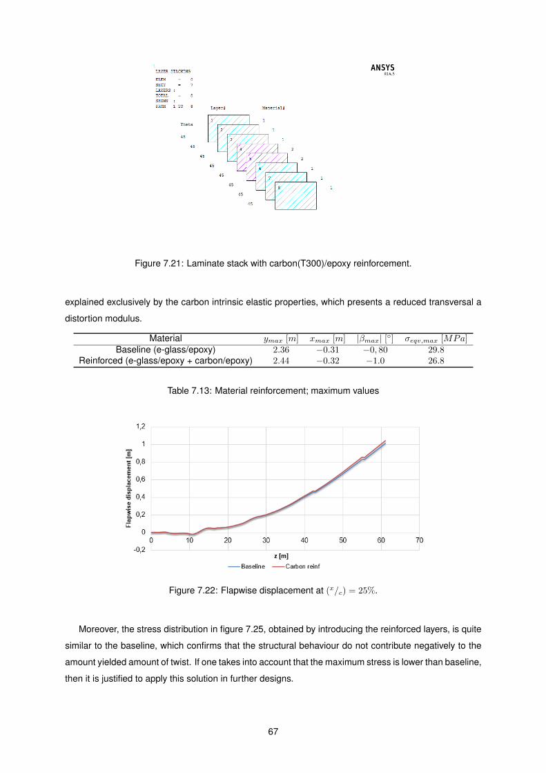
Figure 7.21: Laminate stack with carbon(T300)/epoxy reinforcement.
explained exclusively by the carbon intrinsic elastic properties, which presents a reduced transversal a
distortion modulus.
Material ymax [m] xmax [m] |βmax| [] σeqv,max [MPa]Baseline (e-glass/epoxy) 2.36 −0.31 −0, 80 29.8
Reinforced (e-glass/epoxy + carbon/epoxy) 2.44 −0.32 −1.0 26.8
Table 7.13: Material reinforcement; maximum values
Figure 7.22: Flapwise displacement at (x/c) = 25%.
Moreover, the stress distribution in figure 7.25, obtained by introducing the reinforced layers, is quite
similar to the baseline, which confirms that the structural behaviour do not contribute negatively to the
amount yielded amount of twist. If one takes into account that the maximum stress is lower than baseline,
then it is justified to apply this solution in further designs.
67

Figure 7.23: Edgewise displacement at (x/c) = 25% for material reinforcement.
Figure 7.24: Twist distribution.
Figure 7.25: von Mises stress distribution: material reinforcement.
68

7.8 Parametric Study Summary
All the evaluated parameters proved to the be quite relevant to blade structural behaviour. The fibres
orientation is one parameter that might be adjusted as function of the local required stiffness, and can
provide significant improvements in the overall performance. It was seen that when the fibres are ori-
ented 90, the flapwise stiffness is greatly increased. This kind of stack is useful in regions that are
subjected to high flapwise moments, which is the case of root region [49]. Obviously, this orientation
avoids twist, but it was shown that the root is very resistant to torsional moments, regardless the fibres
orientation, due to its geometrical properties. The remaining blade surface should integrate fibres ori-
ented +45, that can induce the highest amount of twist. As function of the displacement observed 90
fibres may be added to reduce the tip displacement.
The thickness is probably the most sensitive and unpredictable parameter of all studied, and its
refinement should be done very carefully. The results show that thicker laminates should be used near
the root to reduce the maximum flapwise displacement. Twist is sacrificed with this choice, but the
structure integrity in the priority. Followed by other design options, the torsional stiffness increase can
be mitigated.
Concerning the webs analysis, the reason why blades have shear webs was clear. The number
of webs showed no obvious conclusions, though the global structural response is enhanced when the
shear webs are introduced. The questions is whether use one or more webs. That question should be
answered by trying to add more information about an optimal position of single web configuration and
compare with the respective double web configuration. Anyway, theoretically, adding a second web may
be always considered a conservative approach, and that is not an option to discard.
Adding another material with different elastic properties brings a new set of possibilities to improve
the blade design. Looking at the mechanic properties of carbon/epoxy, it would be clever to introduce
it in 90 fibres and take advantage of high longitudinal modulus of this material. Since it also provides
an increase in induced twist, combined with an adequate thickness distribution, then it can be used until
mid-span region, where laminate thickness is still considerable.
69

70

Chapter 8
Enhanced Blade Design
In the last chapter it was possible to collect an amount of data relative to the parameters one should take
in consideration in wind turbine blade design. The parametric study was concluded with clues about an
enhanced version of the blade under study, aiming a mitigation of the aerodynamic load.
8.1 Design properties
Following the sequence of parameters studied in the last chapter, the fibres orientation should be such
way, that it can provide both flapwise stiffness and induced twist on the blade. Therefore, assuming that
the blade root is subjected to high flapwise moments, all layers with 90 fibres (longitudinal direction)
were used, so a high longitudinal stiffness can be achieved with this layup. The root laminate stack is
presented in figure 8.1(a).
Ideally, the remain blade surface should be covered by layers with -45 fibres, but buckling issues
might occur and for that reason, usually real blades have layers with longitudinal fibres [49]. Hence, it
was applied a stack to the blade surface as illustrated in figure 8.1(c).
The region right next to the root, between 10 and 20m, has shown to be region of structural de-
mand, thus two additional longitudinal fibres were replaced from -45, creating an intermediate solution
between root and tip stacks, as illustrated in figure 8.1(b).
The thickness distribution was maintained to the one identified as dist thickness 1 in figure 7.12. The
author believes that the positives effects of new laminate stack, will mitigate adverse effects of having
this thickness distribution, namely the loss of flapwise stiffness.
The shear webs position was changed in relation to the baseline configuration, although the double
web configuration has been maintained. The argument of this modification has to do with the lack of
effectiveness demonstrated by the shear web located closer to the trailing edge. Despite the good
performance evidenced by the single shear web configuration, it is not clear that this performance could
be consistent when a variable thickness distribution is introduced. Furthermore, in the research that
supported this work, the double web configuration is rather used than single one. Further studies would
have be necessary to abandon this conservative solution.
71

(a) Root. (b) Midspan.
(c) Tip.
Figure 8.1: Laminate stacks in different blade regions.
Finally, regarding the reinforcement done in the previous chapter, it revealed to be successful and it
was integrated in the laminates stack, as shown in figures 8.1(a) to ?? labelled by material 2. In root, the
interior layers were changed to the carbon composite, and the remaining blade span, included carbon
fibres not only in the longitudinal layers, but also in the interior layers containing oblique fibres.
8.2 Coupled Analysis
This analysis consisted of a iterative solution, coupling the structural twist ∆β into the aerodynamic
model to obtain an updated surface load, as explained in detail in section 6.3. The simulation has been
ran until the convergence of both displacements and forces have been verified.
8.2.1 Structural Performance
With five iterations was possible to get a converged solution, regarding nodal displacements and twist
distribution.
The results show that the aerodynamic load can effectively be mitigated with this design, and produce
significant reductions in both flapwise and edgwise displacement, which are visible in figures 8.2 and
8.3. The twist distribution in figure 8.4 is also lower when the solution is converged, but that difference
72

Figure 8.2: Enhanced blade: edgewise displacement at (x/c) = 25%.
is not as noticeable, as table 8.2 confirms.
Figure 8.3: Enhanced blade: flapwise displacement displacement at (x/c) = 25%.
Figure 8.4: Enhanced blade: twist distribution.
73

The stress distribution, in figure 8.5 shows that the reinforcement applied after the root region was
not sufficient to mitigate the high stress in that region, although the maximum value exhibited in table
8.1 it is clear lower than the estimated yield strength of composite in the previous chapter. Even though,
since two different materials are being used, the structure will enter in plastic regime when the first of
two materials enter in plastic regime. Hence, it is necessary to guarantee that the maximum stress is not
higher than the carbon/epoxy yield strength. Applying once more equation (7.1), it simple to conclude
that
(σyc)2 ≈ 633.4 MPa, (8.1)
is proportional directly proportional to the composite longitudinal modulus, as the matrix is the same.
The first material to achieve eventual plastic strains is the e-glass/epoxy composite, which is not this
case. Anyway, further investigations should be done in this particular point, as some researchers [10],
[25] affirm that designs implemented high levels of BTC can increase fatigue loads. Therefore, the
impact of this stress in fatigue lifetime should be evaluated.
Figure 8.5: Enhanced blade: von Mises stress plot.
Iteration ymax [m] xmax [m] βmax [] σeqv,max [MPa]1 to 5 2.05 −0.20 1.31 59.2
5 1.35 −0.12 1.14 50.8
Table 8.1: Enhanced blade: maximum values.
The estimated total load in upper and lower blade surfaces were
|F upper(1)| = 87.3 kN and |F lower(1)| = 33.5 kN
74

Iteration ∆ymax [%] ∆ xmax [%] ∆ βmax [%] ∆ σeqv,max [%]5 −35.5 −37.7 −13 −14.2
Table 8.2: Enhanced blade: parameters deviations between first and last iterations.
In the end of coupled analysis, these values were
|F upper(5)| = 85.0 kN and |F lower(5)| = 33.4 kN
Resulting in total aerodynamic load reduction of 2.1%. This result indicates that from modest re-
ductions in aerodynamic load, is possible avoid extreme displacements, verified by the blade, whenever
wind speed is much higher than normal. The benefits may be extended to an increase in blade lifetime.
8.3 Aerodynamic Performance
The aerodynamic parameters are not significantly affected by this enhanced design, nevertheless, it is
visible in both figures 8.6 and 8.7 deviations specially in the second half of span, where the twist is more
appreciable. In the former, that is a direct consequence of the reduction in the angle of attack. The
latter, it is negative effect of induce twist, because the torque exerted on the blade is reduced. Instead
of making the air flow rotate, it is the blade itself that is rotating, losing the rotational kinetic energy that
could be extracted from wind. Therefore, the angular induction factor is lower with this design, which
gives a negative contribution to power production, as can be seen by equation (7.2).
Figure 8.6: Enhanced blade: lift coefficient.
8.4 Static Analysis including Inertial Loads
This final analysis aims to give an insight about the impact of inertial loads on the blade response. This
analysis followed exactly the same procedures of the previous one, but in this case it was considered an
75

Figure 8.7: Enhanced blade: power coefficient.
extreme case, where aerodynamic, gravitational and gyroscopic loads are acting in the same direction,
with the blade parallel to the ground.
The maximum tip deflection used in [49], was 8.46 m, for a rotating situation. In that work, a 70 m
blade was analysed, also developed by NREL, with identical geometrical features. Thus, it is acceptable
to make linear re-scaling to have a reference value about the maximum tip deflection of the blade one is
working. The estimated value was 7.25 m. In [49], it is also applied a safety factor of 1.35 in all forces,
but for convenience, in this analysis it was applied the same safety factor to the maximum tip deflection,
yielding 5.37 m. The reference angular velocity used during the simulations is the rated rotor speed, as
described in table 7.1.
The same trends verified in the previous analysis are visible in figures 8.8 to 8.10. The main dif-
ferences lie on the maximum absolute values, that are quite superior due to the introduction of the
additional sources of load. The reference maximum tip deflection is not reached, but it should be noted
that other types of load can still be added to the ones considered so far, which may induce even higher
displacements.
Figure 8.8: Enhanced blade including inertial loads: flapwise displacement at (x/c) = 25%.
76

Figure 8.9: Enhanced blade including inertial loads: edgewise displacement at (x/c) = 25%.
Figure 8.10: Enhanced blade including inertial loads: twist distribution.
The increase in total load is also reflected on the stress exerted on the blade. The distribution is
similar to the one of analysis, but while in that one the maximum stress clearly below the estimated yield
strength, the actual load yields a maximum much closer to this boundary. Furthermore, applying the
same safety factor to the composite yield strength, in fact this threshold is slightly exceeded. Similarly
as what happens in figure 8.5, from the stress plot in figure 8.11, it is evident an overstressed region
next to the root, due not only to the insertion zone of webs, but also where high suction zones are found.
Therefore, for a more conservative approach, it is prudent, to reinforce this zone either by changing some
of the oblique layers by longitudinal layers or, alternatively, make a slight adjustment in the laminate
thickness.
77

Figure 8.11: Enhanced blade including inertial loads: von Mises stress.
78

Chapter 9
Conclusions
Wind energy is actually one industry in steady evolution and, in the next decades, it is expected that a
significant part of the total yielded clean energy is exclusively extracted from wind. In this context, wind
turbines followed the technological advances and nowadays are quite complex structures, incorporating
not only noble materials but also advanced control systems, aiming power outputs that can justify the
production cost of such devices.
The passive control is a very efficient approach in terms of cost, that can maintain at acceptable
levels the blade power output and reduce the aerodynamic load in case of high wind speeds. The
bend-twist coupling is one technique of passive control that can provide that desired aerodynamic load
mitigation, reducing the wind incidence on the blade. These effects are more noticeable, the greater the
wind speed is.
The selected parameters in the parametric study provide several solutions to produce an enhanced
blade model, and can significantly change both mechanic properties of the blade and the structural
response. They can be adjusted in order to produce the desired effects in terms of the maximum
displacements and in the amount of twist.
The design presented in this work focused in a blade configuration that could provide the maximum
twist possible, in a such way that applying the BTC concept could achieve an effective aerodynamic load
reduction. This reduction is particularly visible in lower maximum displacements and stresses in the
structure.
The developed enhanced design was justified from the findings of a parametric study and confirmed
its proposals. Besides the reduction of total aerodynamic load through the coupling of induced self twist,
both blade flapwise and edgewise maximum deflections were reduced with this design. Taking into
account the reference values and all the developed reasoning, it has been shown that the blade stiffness
was correctly dimensioned, as the maximum stress ranged below the material yield strength.
The integration of inertial loads in the analysis has confirmed that these source of loads are quite
relevant in the design stage, as they represent a significant part of total load exerted upon the blade.
This design maintained enough sturdiness to keep maximum displacements below reference values, so
a sort of static validation of this model was performed successfully.
79

9.1 Achievements
This research allowed a complete, but not exhaustive insight about wind energy. The knowledge about
wind turbines require a lot of different engineering sciences, as aerodynamics, composite materials,
structural mechanics, as many other. Deeper and stronger bases were built in these fields to produce
this report.
A simple mesh generator was developed, capable to compute a parametric structured mesh relative
to a WTB, regardless of its geometry.
The developed aerodynamic model, despite its simplicity, allowed an estimation qualitatively correct
about the pressure distribution.
It was possible to evaluate from a set of parameters what were those who were more relevant to
blade structural behaviour. From the evaluated parameters, it was computed an enhanced design of the
blade under study, that fulfilled the desired goals.
9.2 Future Work
The model developed in the scope of this work should be validated through commercial codes. They
typically rather evolve all WT components than exclusively the blade, therefore extrapolations to the
developed model should be done.
In this work, the emphasis is given to the aerodynamic load, and a brief analysis with inertial loads
was made. Further advances should be done in this field, adding others source of load, and considering
non-linear components. It would be interesting to implement stochastic models, already existent repre-
sentative of the non-periodic wind loads. The study of the impact of fatigue loads, in this context, will be
very useful.
During the parametric study some questions were not answered. The ideal number and the position
of shear webs became inconclusive, and further studies are needed to have clear picture about this
particular point. A buckling analysis, crossing all the gathered data will also add value to this research
The aerodynamic model should suffer several improvements, particularly the pressure distribution in
root, which the estimation is very rough. Other types of tools, as CFD codes, should be employed to
have more precise load distributions.
The developed FSI model should take into account the mesh deformation in further iterations to be
truly considered a loose coupling method.
80

Bibliography
[1] Brian R Resor. Definition of a 5MW / 61 . 5m Wind Turbine Blade Reference Model. 2013.
[2] D Otero, F L Ponta, and L I Lago. Structural Analysis of Complex Wind Turbine Blades: Flexo-
Torsional Vibrational Modes. Advances in Wind Power, 2012. doi: 10.5772/51142.
[3] Pengwen Sun, Zhifu Liu, Yongguang Gao, and Sheng Wu. Lay-up Design and Structural Analysis
of 1.2MW Composite Wind Turbine Blade. 2009. 9781424452682.
[4] Prospector Materials database. https://www.ulprospector.com/en/na. Energy Procedia,
(1876):194–201. Visited in May 2015.
[5] Manudha T. Herath, Aaron K.L. Lee, and B. Gangadhara Prusty. Design of shape-adaptive wind
turbine blades using differential stiffness bend-twist coupling. Ocean Engineering, 95:157–165,
February 2015. doi: 10.1016/j.oceaneng.2014.12.010.
[6] Low Tech Magazine. http://www.lowtechmagazine.com/2009/10/history-of-industrial-
windmills.html. Visited in February 2015.
[7] Erich au. Wind turbines: Fundamentals, technologies, application, economics. Springer, 3rd edi-
tion, 2006. ISBN 10.1007/3-540-29284-5.
[8] European Wind Energy Association. http://www.ewea.org/. Visited in February 2015.
[9] J. F. Manwell, J. G. McGowan, and A. L. Rogers. Wind Energy Explained. John Wiley & Sons LTD,
2nd edition, 2009. ISBN 978-0-470-01500-1.
[10] W.C. de Goeij, M.J.L. van Tooren, and A. Beukers. Implementation of bending-torsion coupling in
the design of a wind turbine rotor blade. Journal of Applied Energy, 2:191–207, 1999.
[11] D M May, S J Jones, and H Crockard. Fundamental of Aerodynamics. Journal of neurosurgery,
85(4):566–573, 1996.
[12] John D. Anderson. Fundamentals of Aerodynamics. Mc Graw Hill, 3rd edition, 2001. ISBN 0-07-
237335-0.
[13] Tony Burton, David Sharpe, Nick Jenkins, and Ervin Bossanyi. Wind Energy Hand Book. John
Wiley & Sons LTD, 2001. ISBN 0 471 48997 2.
81

[14] Martin O. L. Hansen. Aerodynamics of Wind Turbines. EARTHSCAN, 2 edition, 2008. 978-1-
84407-438-9.
[15] ANSYS. Theory Reference for the Mechanical APDL and Mechanical Applications. 12th edition,
2009.
[16] J.N. Reddy. Mechanics of Laminated Composite Plates and Shells. CRC PRESS, 2nd edition,
2004. ISBN 0849315921.
[17] Galina Seiber. Numerical simulation of fluid-structure interaction using loose coupling methods.
Master’s thesis, Technischen Universitat Darmstadt, 2002.
[18] Dong Ok Yu and Oh Joon Kwon. Predicting wind turbine blade loads and aeroelastic response
using a coupled CFD-CSD method. 70:184–196, 2014. doi: 10.1016/j.renene.2014.03.033.
[19] Vasco Brederode. Fundamentos de Aerodinamica Incompressivel. Edicao de autor, 1997.
[20] Peter J. Schubel and Richard J. Crossley. Wind turbine blade design. Energies, 5(9):3425–3449,
2012. doi: 10.3390/en5093425.
[21] Wen-Hsiang Wu and Wen-Bin Young. Structural Analysis and Design of the Composite Wind Tur-
bine Blade. Applied Composite Materials, 19(3-4):247–257, 2012. doi: 10.1007/s10443-011-9193-
z.
[22] Wang Xudong. Shape optimization of wind turbine blades. Wind Energy, 12(8):781–803, 2009.
doi: 10.1002/we.335.
[23] Niels Troldborg and Jn Sø rensen. Numerical validation of a finite elment thin-walled beam model
of a composite wind turbine blade. Wind Energy, 15:203–223, 2012. doi: 10.1002/we.
[24] Wenping Cao, Ying Xie, and Zheng Tan. Wind Turbine Generator Technologies. INTECH, 2012.
doi: http://dx.doi.org/10.577251780.
[25] Don W. Lobitz and Paul S. Veers. Load Mitigation with Bending/Twist-coupled Blades on Rotors
using Modern Control Strategies. Wind Energy, 6(2):105–117, 2003. doi: 10.1002/we.74.
[26] Scott J Johnson, C P Case Van Dam, and Dale E Berg. Active Load Control Techniques for Wind
Turbines. SANDIA NATIONAL LABORATORIES,, 2008.
[27] Dale E. Berg, Jose R. Zayas, Donald W. Lobitz, C. P. van Dam, Raymond Chow, and Jonathon P.
Baker. Active Aerodynamic Load Control of Wind Turbine Blades. Fluid Dynamics Conference,
pages 1119–1127, 2007. doi: 10.1115/FEDSM2007-37604.
[28] Matthew A Lackner and Mario A Rotea. Passive structural control of offshore wind turbines. Wind
Energy, 14:373–388, 2011. doi: 10.1002/we.
[29] E Muljadi, K Pierce, P Migliore, National Wind, and National Renewable. Control strategy for
varaible-speed Stall-Regulated Wind Turbines. NREL Laboratories, 1998.
82

[30] Dimitris Bourlis. A Complete Control Scheme for Variable Speed Stall Regulated Wind Turbines.
INTECH, 2007. University of Leicester.
[31] Christian Deilmann. Passive aeroelastic tailoring of wind turbine blades - A numerical analysis -.
Master’s thesis, Massachussets Institute of Technology, 2009.
[32] V Fedorov and C Berggreen. Bend-twist coupling potential of wind turbine blades. Journal of
Physics: Conference Series, 524:012035, 2014. doi: 10.1088/1742-6596/524/1/012035.
[33] Tom Ashwill. Passive Load Control for Large Wind Turbines. 51st AIAA/ASME/ASCE/AH-
S/ASC Structures, Structural Dynamics, and Materials Conference, pages 1–12, 2010. doi:
10.2514/6.2010-2577.
[34] Andrew T Lee, B E Hons, and Richard G J Flay. Compliant blades for wind turbines. IPENZ
Conference, 1998.
[35] Georgios Pechlivanoglou. Passive and active flow control solutions for wind turbine blades. PhD
thesis, Technischen Universitat Berlin, 2013.
[36] XFOIL. http://web.mit.edu/aeroutil v1.0/xfoil doc.txt. . Visited in March 2015.
[37] M. Drela. XFOIL 6.94 User Guide. 2001.
[38] Aerodynamics for Students. http://www-mdp.eng.cam.ac.uk/web/library/
enginfo/aerothermal dvd only/aero/fprops/poten/node37.html. Visited in March 2015.
[39] G. P. Nikishkov. Introduction To The Finite Element Method. Lecture Notes UCLA, 12 edition, 2004.
[40] CFD-Online. http://www.cfd-online.com/wiki/mesh classification. Visited in May 2015.
[41] S A Brown. Displacement Extrapolations for CFD+CSM Aeroelastic Analysis. 97(1090):291–300,
1997.
[42] Ramji Kamakoti and Wei Shyy. Fluid-structure interaction for aeroelastic applications. Progress in
Aerospace Sciences, 40(8):535–558, 2004. doi: 10.1016/j.paerosci.2005.01.001.
[43] Mauwafak a Tawfik, Mohammed I Abu-tabikh, and Farouk O Hamdoon. Aeroelastic behavior of a
wind turbine blade by a fluid -structure interaction analysis. Al- Khwarizmi Engineering, 9(3):15–25,
2013.
[44] Timur Alexeev. Computational Aeroelasticity Study of Horizontal Axis Wind Turbines with Coupled
Bending-Torsion Blade Dynamics. PhD thesis, 2013.
[45] J Jonkman, S Butterfield, W Musial, G Scott, J Jonkman, S Butterfield, W Musial, and G Scott. Defi-
nition of a 5-MW Reference Wind Turbine for Offshore System Development. 2009. doi: 10.1002/a-
jmg.10175.
[46] Emad S Al-hasani. Study of tensile strength and hardness property for epoxy reinforced with glass
fiber layers. Eng. & Technology, 25(8):988–997, 2007.
83

[47] K Devendra and T Rangaswamy. Strength characterization of e-glass fiber reinforced epoxy com-
posites with filler materials. Minerals and Materials Characterization and Engineering, 1:353–357,
2013.
[48] Barrie S. H. Royce. http://www.princeton.edu/maelabs/mae324/11/11mae 21.htm. Visited in May
2015.
[49] Kevin Cox and Andreas Echtermeyer. Structural design and analysis of a 10MW wind turbine blade.
Energy Procedia, 24(1876):194–201, 2012. doi: 10.1016/j.egypro.2012.06.101.
[50] Jorge Rodrigues and Paulo Martins. Tecnologia Mecanica Vol 1 - Tecnologia da deformacao
plastica. Platano editora, 2010.
84

Appendix A
A.1 von Mises Failure Criterion
The von Mises failure is satisfied if von Mises equivalent stress σv is higher than the yield strength of the
material. von Mises equivalente stress is given by [50]
σv =
[(σ1 − σ2)2 + σ2 − σ3)2 + σ3 − σ1)2
2
]1/2. (A.1)
The von Mises failure criterion is satisfied when
σv ≥ σy. (A.2)
A.2 Thin Airfoil Theory
An airfoil is defined by first drawing a mean camber line. The straight line that joins the leading and
trailing ends of the mean camber line is called the chord line. The length of the chord line is called
chord, c. To the mean camber line, a thickness distribution is added in a direction normal to the camber
line to produce the final airfoil shape. Equal amounts of thickness are added above the camber line, and
below the camber line [12].
Figure A.1: Main airfoil geometric definitions (reproduced from [19]).
An airfoil with no camber (i.e. a flat straight line for camber) is a symmetric airfoil. The angle that a
freestream makes with the chord line is called the angle of attack, α.
Let Y be the pressure force per unit span along the Y- axis. This force may be computed as
85

Y =
∫lower
pdx−∫upper
pdx =
∫(pupper − plower)dx. (A.3)
We can now yield a non-dimensional form, from the above dimensional expression, by dividing the
pressure by the dynamic pressure, and the distances by the chord c. Then:
CY =Y
12ρU
2c=
∫[(pupper − p0)− (plower − p0)]
12ρU
2cdx
c=
∫(CP,upper − CP,lower)d
x
c. (A.4)
We can likewise find the component of force acting along the x- axis. This force and its non-
dimensional form are given by
X =
∫pupper
(dY
dx
)upper
dx−∫plower
(dY
dx
)lower
dx, (A.5)
CX =X
12ρU
2c=
∫ [CP,upper
(dY
dx
)upper
− CP,lower(dY
dx
)lower
]dx
c. (A.6)
The X and Y- forces act along the x- and y- axes, respectively. Lift is defined as the component
of pressure force that is normal to the freestream direction, and drag is defined as the component of
pressure force along the freestream direction. If the airfoil was initially located so that the chord line is
along the x- axis, then the angle between the freestream direction and the x- axis is the angle of attack
α.
Lift and drag are related to the X- and Y- forces as
L = Y cosα−Xsinα, (A.7)
D = Xcosα+ Y sinα, (A.8)
Cl = CY cosα− CXsinα, (A.9)
Cd = CXcosα+ CY sinα. (A.10)
The quantities Cl and Cd are called the lift, and drag coefficients, respectively. By convention, the
lower case subscripts are used in 2-D flows, while upper case subscripts are used to denote lift and drag
coefficients of three-dimensional configurations such as wings.
We can also define the pitching moment about any point on the chord line. Nose up moment is
considered positive. About a general point on the x- axis whose co-ordinates are given by (a,0), the
pitching moment per unit span is given in dimensional and non-dimensional forms respectively by
M =
∫(plower − pupper)(x− a)dx, (A.11)
86

Figure A.2: Aerodynamic forces: lift and drag (reproduced from [19]).
Cm =
∫(cP,lower − CP,upper)(
x
c− a
c)dx
c. (A.12)
While the pitching moment can be defined about any point in space, it is customary to compute the
pitching moment M and the pitching moment coefficient Cm about the quarter chord, i.e. a location
25% downstream of the leading edge.
The centre of pressure is defined as the point about which the pitching moment is zero. As the flow
conditions change (example, angle of attack α changes), the centre of pressure will change.
The aerodynamic centre is defined as the point where the pitching moment (or the pitching moment
coefficient) is independent of α. That is, if we computed the pitching moment about the aerodynamic
centre:
∂M
∂α=∂Cm∂α
= 0. (A.13)
The thin airfoil theory yields the following results:
Cl = 2π(α− α0),∂Cl∂α
= 2π, (A.14)
Cd = 0, (A.15)
∂Cm∂α
= 0, at 25% of chord. (A.16)
The quantity α0 is called the angle of zero lift.. In real flows, Cl, Cd and Cm will differ from this theory,
due to viscous effects. As may be expected, symmetric airfoils will have zero lift at zero angle of attack.
Thus, α0 is zero for symmetric airfoils. For cambered airfoils α0 can have positive or negative, depending
on whether they have a positive (curved up) or negative camber (curved down).
87

Appendix B
B.1 Matlab APDL Code Generator
1 %%%%%%Output F i l e%%%%%%%%%
2
3 c l c ;
4
5
6 %%
7 %%Mate r i a l P rope r t i es
8
9 Ex=43.2e9 ;
10 Ey=12.6e9 ;
11 Ez=12.6e9 ;
12 Gxy=4.2e9 ;
13 Gxz=4.2e9 ;
14 Gyz=4.2e9 ;
15 vL =0.28;
16 dens=1920;
17
18 f i d = fopen ( ’ output MATLAB . t x t ’ , ’ wt ’ ) ;
19
20 %t i t l e
21 f p r i n t f ( f i d , ’ ! Edgar Carro lo \n ! Wind Turbine Blade FEM\n ’ ) ;
22
23 %White screen
24 f p r i n t f ( f i d , ’ FINISH\n /CLEAR, ALL \n /PREP7 \n /RGB, INDEX,100 ,100 ,100 , 0 \n
/RGB, INDEX , 80 , 80 , 80 ,13 \n /RGB, INDEX , 60 , 60 , 60 ,14 \n /RGB, INDEX , 0 ,
0 , 0 ,15 \n /REPLOT\n ’ ) ;
25
88

26
27
28 f p r i n t f ( f i d , ’MPTEMP, , , , , , , , \n MPTEMP,1 ,0 \n MPDATA,EX,1 , ,% f \n MPDATA,EY
,1 , ,% f \n MPDATA, EZ,1 , ,% f \n MPDATA,PRXY,1 , ,% f \n MPDATA,PRYZ, 1 , , \n
MPDATA,PRXZ, 1 , , \n MPDATA,GXY,1 , ,% f \n MPDATA,GYZ,1 , ,% f \n MPDATA,GXZ
,1 , ,% f \n MPTEMP, , , , , , , , \n MPTEMP,1 ,0 \n MPDATA,DENS,1 , ,%d \n ’ ,Ex , Ey ,
Ez , vL , Gxz , Gyz , Gxy , dens ) ;
29
30 %%
31 %Element Prope r t i es
32 f p r i n t f ( f i d , ’ ET,1 ,SHELL181\n KEYOPT,1 ,1 ,0\n KEYOPT,1 ,3 ,2 \nKEYOPT,1 ,8 ,2 \
nKEYOPT,1 ,9 ,0\n ’ ) ;
33
34 %% Thickness d i s t r i b u t i o n
35 t1 =0.0125;
36 t2 =0.0025;
37 t3 =0.005625;
38 t4 =0.00375;
39 t5 =0.00375;
40 t6 =0.0025;
41 t7 =0.0025;
42
43 f p r i n t f ( f i d , ’ \n t1 =0.0125\n t2 =0.0025 \n t3 =0.005625 \n t4 =0.00375 \n t5
=0.00375 \n t6 =0.0025 \n t7 =0.0025 ’ ) ;
44
45
46 %%
47 %%Composite stack and f i b r e l aye r o r i e n t a t i o n
48
49 f p r i n t f ( f i d , ’ \nsect , 1 , she l l , , r oo t \n secdata , t1 ,1 ,90 ,3 \n secdata , t1 ,1 ,90 ,3
\n secdata , t1 ,1 ,25 ,3 \n secdata , t1 ,1 ,−45 ,3 \n secdata , t1 ,1 ,−45 ,3 \n
secdata , t1 ,1 ,25 ,3 \n secdata , t1 ,1 ,90 ,3 \n secdata , t1 ,1 ,90 ,3 \n
seccont ro l ,0 ,0 ,0 ,0 ,1 ,1 ,1 \n seco f f se t , MID ’ ) ;
50 f p r i n t f ( f i d , ’ \nsect , 2 , she l l , , web \n secdata , t2 ,1 ,90 ,3 \n secdata , t2 ,1 ,90 ,3
\n secdata , t2 ,1 ,25 ,3 \n secdata , t2 ,1 ,−45 ,3 \n secdata , t2 ,1 ,−45 ,3 \n
secdata , t2 ,1 ,25 ,3 \n secdata , t2 ,1 ,90 ,3 \n secdata , t2 ,1 ,90 ,3 \n \n \n
seco f f se t , MID \n seccont ro l ,0 ,0 ,0 ,0 ,1 ,1 ,1 \n ’ ) ;
51 f p r i n t f ( f i d , ’ \nsect , 3 , she l l , , sec1 \n secdata , t3 ,1 ,90 ,3 \n secdata , t3
,1 ,90 ,3 \n secdata , t3 ,1 ,25 ,3 \n secdata , t3 ,1 ,−45 ,3 \n secdata , t3 ,1 ,−45 ,3
89

\n secdata , t3 ,1 ,25 ,3 \n secdata , t3 ,1 ,90 ,3 \n secdata , t3 ,1 ,90 ,3 \n
seco f f se t , MID \n seccont ro l ,0 ,0 ,0 ,0 ,1 ,1 ,1 ’ ) ;
52 f p r i n t f ( f i d , ’ \nsect , 4 , she l l , , sec2 \n secdata , t4 ,1 ,90 ,3 \n secdata , t4 ,1 ,90 ,3
\n secdata , t4 ,1 ,25 ,3 \n secdata , t4 ,1 ,−45 ,3 \n secdata , t4 ,1 ,−45 ,3 \n
secdata , t4 ,1 ,25 ,3 \n secdata , t4 ,1 ,90 ,3 \n secdata , t4 ,1 ,90 ,3 \n seco f f se t
, MID \n seccont ro l ,0 ,0 ,0 ,0 ,1 ,1 ,1 ’ ) ;
53 f p r i n t f ( f i d , ’ \nsect , 5 , she l l , , sec3 \n secdata , t5 ,1 ,90 ,3 \n secdata , t5 ,1 ,90 ,3
\n secdata , t5 ,1 ,25 ,3 \n secdata , t5 ,1 ,−45 ,3 \n secdata , t5 ,1 ,−45 ,3 \n
secdata , t5 ,1 ,25 ,3 \n secdata , t5 ,1 ,90 ,3 \n secdata , t5 ,1 ,90 ,3 \n seco f f se t
, MID \n seccont ro l ,0 ,0 ,0 ,0 ,1 ,1 ,1 ’ ) ;
54 f p r i n t f ( f i d , ’ \nsect , 6 , she l l , , sec4\n secdata , t6 ,1 ,90 ,3 \n secdata , t6 ,1 ,90 ,3
\n secdata , t6 ,1 ,25 ,3 \n secdata , t6 ,1 ,−45 ,3 \n secdata , t6 ,1 ,−45 ,3 \n
secdata , t6 ,1 ,25 ,3 \n secdata , t6 ,1 ,90 ,3 \n secdata , t6 ,1 ,90 ,3 \n seco f f se t
, MID \n seccont ro l ,0 ,0 ,0 ,0 ,1 ,1 ,1 ’ ) ;
55 f p r i n t f ( f i d , ’ \nsect , 7 , she l l , , sec5 \n secdata , t7 ,1 ,90 ,3 \n secdata , t7 ,1 ,90 ,3
\n secdata , t7 ,1 ,25 ,3 \n secdata , t7 ,1 ,−45 ,3\n secdata , t7 ,1 ,−45 ,3 \n
secdata , t7 ,1 ,25 ,3 \n secdata , t7 ,1 ,90 ,3 \n secdata , t7 ,1 ,90 ,3 \n seco f f se t
, MID \n seccont ro l ,0 ,0 ,0 ,0 ,1 ,1 ,1 \n ’ ) ;
56
57
58 %%
59 %Node generat ion
60
61 [ y , b ]= s ize (mesh) ;
62 f p r i n t f ( f i d , ’ ! Keypoints L i s t \n !\n ’ ) ;
63 f o r l =1 :1 : y
64 f p r i n t f ( f i d , ’N, %d , %f , %f , %f ! \n ’ , l , mesh( l , 2 ) ,mesh( l , 3 ) ,mesh( l , 4 ) )
;
65 end
66
67 %%
68 %Element generat ion
69
70 [ y , b ]= s ize (A) ;
71 f p r i n t f ( f i d , ’ !\n ! Elements L i s t \n !\n ’ ) ;
72
73 f o r l =1 :1 : y
74 f p r i n t f ( f i d , ’E , %d , %d , %d , %d ! \n ’ ,A( l , 1 ) ,A( l , 2 ) ,A( l , 3 ) ,A( l , 4 ) ) ;
75 end
90

76
77 %%
78 %Assignement o f the ma te r i a l p r o p e r t i e s to the respec t i ve set o f elements
79 f p r i n t f ( f i d , ’ESEL, ALL\n ’ ) ;
80 f p r i n t f ( f i d , ’EMODIF, ALL ,SECNUM,2\n ’ ) ;
81
82 f p r i n t f ( f i d , ’ \nESEL,ELEM,1 ,%d\n ’ ,max( sec roo t ) ) ;
83 f p r i n t f ( f i d , ’EMODIF, ALL ,SECNUM,1\n ’ ) ;
84
85 sec roo t2=max( sec roo t ) +n elemz∗n elemc ;
86 f p r i n t f ( f i d , ’ \nESEL,ELEM,%d,%d\n ’ , n elemc∗n elemz +1 , sec roo t2 ) ;
87 f p r i n t f ( f i d , ’EMODIF, ALL ,SECNUM,1\n ’ ) ;
88
89 f p r i n t f ( f i d , ’ \nESEL,ELEM,%d,%d\n ’ , sec num1 ( 1 ) ,max( sec num1 ) ) ;
90 f p r i n t f ( f i d , ’EMODIF, ALL ,SECNUM,3\n ’ ) ;
91
92 sec2 num1=max( sec num1 ) +n elemz∗n elemc ;
93 f p r i n t f ( f i d , ’ \nESEL,ELEM,%d,%d\n ’ , n elemc∗n elemz+sec num1 ( 1 ) , sec2 num1 ) ;
94 f p r i n t f ( f i d , ’EMODIF, ALL ,SECNUM,3\n ’ ) ;
95
96 f p r i n t f ( f i d , ’ \nESEL,ELEM,%d,%d\n ’ , sec num2 ( 1 ) ,max( sec num2 ) ) ;
97 f p r i n t f ( f i d , ’EMODIF, ALL ,SECNUM,4\n ’ ) ;
98
99 sec2 num2=max( sec num2 ) +n elemz∗n elemc ;
100 f p r i n t f ( f i d , ’ \nESEL,ELEM,%d,%d\n ’ , n elemc∗n elemz+sec num2 ( 1 ) , sec2 num2 ) ;
101 f p r i n t f ( f i d , ’EMODIF, ALL ,SECNUM,4\n ’ ) ;
102
103 f p r i n t f ( f i d , ’ \nESEL,ELEM,%d,%d\n ’ , sec num3 ( 1 ) ,max( sec num3 ) ) ;
104 f p r i n t f ( f i d , ’EMODIF, ALL ,SECNUM,5\n ’ ) ;
105
106 sec2 num3=max( sec num3 ) +n elemz∗n elemc ;
107 f p r i n t f ( f i d , ’ \nESEL,ELEM,%d,%d\n ’ , n elemc∗n elemz+sec num3 ( 1 ) , sec2 num3 ) ;
108 f p r i n t f ( f i d , ’EMODIF, ALL ,SECNUM,5\n ’ ) ;
109
110 f p r i n t f ( f i d , ’ \nESEL,ELEM,%d,%d\n ’ , sec num4 ( 1 ) ,max( sec num4 ) ) ;
111 f p r i n t f ( f i d , ’EMODIF, ALL ,SECNUM,6\n ’ ) ;
112
113 sec2 num4=max( sec num4 ) +n elemz∗n elemc ;
114 f p r i n t f ( f i d , ’ \nESEL,ELEM,%d,%d\n ’ , n elemc∗n elemz+sec num4 ( 1 ) , sec2 num4 ) ;
91

115 f p r i n t f ( f i d , ’EMODIF, ALL ,SECNUM,6\n ’ ) ;
116
117 f p r i n t f ( f i d , ’ \nESEL,ELEM,%d,%d\n ’ , sec num5 ( 1 ) ,max( sec num5 ) ) ;
118 f p r i n t f ( f i d , ’EMODIF, ALL ,SECNUM,7\n ’ ) ;
119
120 sec2 num5=max( sec num5 ) +n elemz∗n elemc ;
121 f p r i n t f ( f i d , ’ \nESEL,ELEM,%d,%d\n ’ , n elemc∗n elemz+sec num5 ( 1 ) , sec2 num5 ) ;
122 f p r i n t f ( f i d , ’EMODIF, ALL ,SECNUM,7\n ’ ) ;
123
124 f p r i n t f ( f i d , ’ \nESEL,ELEM,%d,%d\n ’ , sect2 elem ( 1 ) , sect2 elem ( sect2 num ) ) ;
125 f p r i n t f ( f i d , ’EMODIF, ALL ,SECNUM,2\n ’ ) ;
126
127
128 %%
129 %Cons t ra in ts
130 k =1;
131 f p r i n t f ( f i d , ’ !\n ! Nodal Const ra in a t blades roo t \n !\n ’ ) ;
132 f o r i =1:1:2∗ n elemz+2
133 f o r j =1:1:2∗ n elemc+2
134 i f mesh( k , 4 ) == 0
135 f p r i n t f ( f i d , ’ d,%d , a l l \n ’ , k ) ;
136 end
137 i f k <= 2∗n elemc∗n elemz+2
138 k=k +1;
139 else
140 break ;
141 end
142 end
143 end
144
145 f p r i n t f ( f i d , ’ \nESEL, ALL ’ ) ;
146
147 %%
148 %Force assignment to each elemnet
149
150 f o r i =1 :1 : n elemz∗n elemc
151 f p r i n t f ( f i d , ’ \nESEL,ELEM,%d , ’ , i ) ;
152 f p r i n t f ( f i d , ’ \nSFE, ALL ,2 ,PRES, ,% f , , , ’ ,F ( i ) ) ;
153 end
92

154
155 f o r i =n elemz∗n elemc +1:1 : n elemz∗n elemc∗2
156 f p r i n t f ( f i d , ’ \nESEL,ELEM,%d , ’ , i ) ;
157 f p r i n t f ( f i d , ’ \nSFE, ALL ,1 ,PRES, ,% f , , , ’ ,F ( i ) ) ;
158 end
159
160 f p r i n t f ( f i d , ’ \nESEL, ALL ’ ) ;
161 f c l o s e ( f i d ) ;
93

94