path coordination guide for the 71-76 and 81-86 ghz
TRANSCRIPT

Wireless Communications Association International 1333 H St., NW Suite 700-W
Washington, D.C. 20005 ph. 202-452-7823 fax. 202-452-0041
Website: www.wcai.com
Path Coordination Guide for the 71-76 and 81-86 GHz
Millimeter Wave Bands
WCA 60+ GHz Committee Version 1.0 June 2004
WCA Document number: WCA-PCG-7080-1

WCA-PCG-7080-1, Rev. 1.0 June 2004
© 2004 Wireless Communications Association International Page ii
Modification History
Revision Date Comments
1.0 June 2004 Initial Version
Copyright © 2004 by the Wireless Communications Association International All rights reserved. No part of this publication may be reproduced, stored in a retrieval system, or transmitted by any means (electronic mechanical, photocopying, recording or otherwise) without written permission of the publisher. Organizations may obtain permission to reproduce a limited number of copies through entering into a license agreement with WCAI. Interested organizations should contact: WCAI Engineering Committee Chair, 1333 H St., NW Suite 700-W, Washington, D.C. 2005. � 1-202-452-7823

WCA-PCG-7080-1, Rev. 1.0 June 2004
© 2004 Wireless Communications Association International Page iii
Table of Contents
1 Introduction..............................................................................................................................1 1.1 Limitations on Document Scope ........................................................................................1 1.2 Areas for Further Study ......................................................................................................1
2 System Overview......................................................................................................................3 2.1 System Description.............................................................................................................3 2.2 Interfaces.............................................................................................................................4 2.3 Interference Scenarios.........................................................................................................5
2.3.1 Case A—Mainbeam- to-Mainbeam and Sidelobe-to-Mainbeam Interference in Clear Weather .............6 2.3.2 Case B—Main-Beam-to-Main-Beam Interference in Rain (Correlated Fading) ......................................6 2.3.3 Case C—Sidelobe-to-Main-Beam Interference in Rain (Uncorrelated Rain Fading)...............................7 2.3.4 Case D—Sidelobe-to-Sidelobe Co-sited Transmitter Interference...........................................................8 2.3.5 Case E—Hub-and-Spoke Interference with Short-Range Links...............................................................9 2.3.6 Case F—Hub-and-Spoke Interference During Precipitation ....................................................................9 2.3.7 Case G—Interference from Other Services............................................................................................10
3 Technical Considerations for Path Design ..........................................................................11 3.1 Introduction.......................................................................................................................11 3.2 Calculation of Interference Levels....................................................................................11 3.3 Objectives for Digital Modulation....................................................................................13
3.3.1 Digital Transmitter Interfering with Digital Victim Receiver ................................................................13 3.3.2 Analog Transmitter Interfering with Digital Victim Receiver................................................................14
3.4 Objectives for Analog Modulation ...................................................................................14 3.5 Propagation Models..........................................................................................................14
3.5.1 Free Space Pathloss................................................................................................................................14 3.5.2 Atmospheric Absorption Losses.............................................................................................................15 3.5.3 Precipitation Losses ...............................................................................................................................15
3.5.3.1 Rainfall Model ................................................................................................................................15 3.5.3.2 Calculation of Rain Attenuation......................................................................................................17 3.5.3.3 Rain Cell Model ..............................................................................................................................19 3.5.3.4 Calculation of Total Attenuation of a Path with Raincell Model ....................................................21
3.5.4 Precipitation Induced Depolarization.....................................................................................................23 3.5.5 Fog Loss.................................................................................................................................................25 3.5.6 Snow and Ice Loss..................................................................................................................................25 3.5.7 RF Backscatter Due to Precipitation ......................................................................................................26 3.5.8 Over-the-Horizon Loss...........................................................................................................................27 3.5.9 Building Obstruction Loss......................................................................................................................28
3.6 Building and Tower Sway ................................................................................................28 3.6.1 Building Sway........................................................................................................................................28 3.6.2 Tower Sway............................................................................................................................................29
3.7 Antenna RPE Smearing Due to Geographic Coordinate Inaccuracy................................30 3.8 Recommended ATPC Behavior .......................................................................................31
4 Terrestrial Service Path Coordination Process...................................................................33 4.1 Link Registration Parameters ...........................................................................................33
4.1.1 Measurement and Input of Site Coordinates ..........................................................................................33 4.1.2 Administrative and Geographic Parameters ...........................................................................................33 4.1.3 Antenna and Radio Equipment Parameters ............................................................................................34 4.1.4 Other Parameters Obtained from Radio and Antenna Vendor ...............................................................34 4.1.5 Parameters Supplied by Path Coordinator..............................................................................................36
4.2 Engineering Analysis........................................................................................................36 4.2.1 Objective of the Analysis .......................................................................................................................36
WCA-PCG-7080-1, Rev. 1.0 June 2004
© 2004 Wireless Communications Association International Page iv
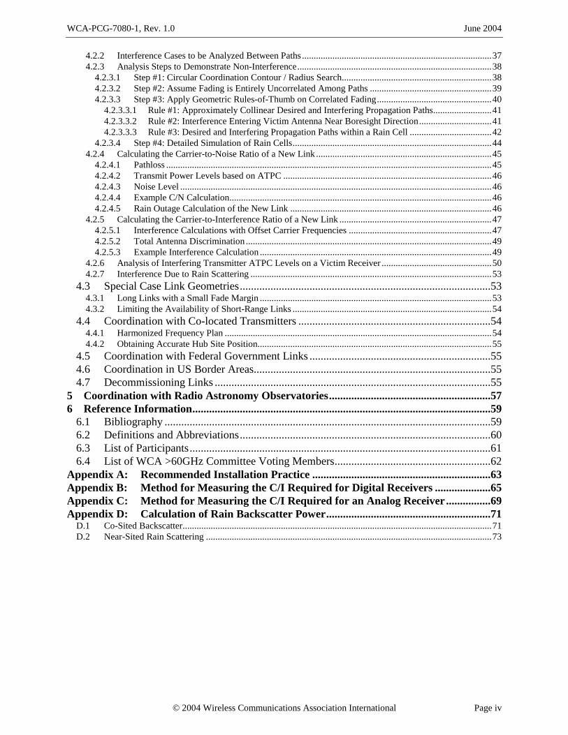
4.2.2 Interference Cases to be Analyzed Between Paths.................................................................................37 4.2.3 Analysis Steps to Demonstrate Non-Interference...................................................................................38
4.2.3.1 Step #1: Circular Coordination Contour / Radius Search................................................................38 4.2.3.2 Step #2: Assume Fading is Entirely Uncorrelated Among Paths ....................................................39 4.2.3.3 Step #3: Apply Geometric Rules-of-Thumb on Correlated Fading.................................................40
4.2.3.3.1 Rule #1: Approximately Collinear Desired and Interfering Propagation Paths.........................41 4.2.3.3.2 Rule #2: Interference Entering Victim Antenna Near Boresight Direction...............................41 4.2.3.3.3 Rule #3: Desired and Interfering Propagation Paths within a Rain Cell ...................................42
4.2.3.4 Step #4: Detailed Simulation of Rain Cells.....................................................................................44 4.2.4 Calculating the Carrier-to-Noise Ratio of a New Link ...........................................................................45
4.2.4.1 Pathloss ...........................................................................................................................................45 4.2.4.2 Transmit Power Levels based on ATPC .........................................................................................46 4.2.4.3 Noise Level .....................................................................................................................................46 4.2.4.4 Example C/N Calculation................................................................................................................46 4.2.4.5 Rain Outage Calculation of the New Link ......................................................................................46
4.2.5 Calculating the Carrier-to-Interference Ratio of a New Link .................................................................47 4.2.5.1 Interference Calculations with Offset Carrier Frequencies .............................................................47 4.2.5.2 Total Antenna Discrimination.........................................................................................................49 4.2.5.3 Example Interference Calculation ...................................................................................................49
4.2.6 Analysis of Interfering Transmitter ATPC Levels on a Victim Receiver ...............................................50 4.2.7 Interference Due to Rain Scattering .......................................................................................................53
4.3 Special Case Link Geometries..........................................................................................53 4.3.1 Long Links with a Small Fade Margin ...................................................................................................53 4.3.2 Limiting the Availability of Short-Range Links .....................................................................................54
4.4 Coordination with Co-located Transmitters .....................................................................54 4.4.1 Harmonized Frequency Plan ..................................................................................................................54 4.4.2 Obtaining Accurate Hub Site Position....................................................................................................55
4.5 Coordination with Federal Government Links .................................................................55 4.6 Coordination in US Border Areas.....................................................................................55 4.7 Decommissioning Links ...................................................................................................55
5 Coordination with Radio Astronomy Observatories..........................................................57 6 Reference Information...........................................................................................................59
6.1 Bibliography .....................................................................................................................59 6.2 Definitions and Abbreviations..........................................................................................60 6.3 List of Participants............................................................................................................61 6.4 List of WCA >60GHz Committee Voting Members........................................................62
Appendix A: Recommended Installation Practice ................................................................63 Appendix B: Method for Measuring the C/I Required for Digital Receivers ....................65 Appendix C: Method for Measuring the C/I Required for an Analog Receiver ................69 Appendix D: Calculation of Rain Backscatter Power...........................................................71
D.1 Co-Sited Backscatter....................................................................................................................................71 D.2 Near-Sited Rain Scattering ..........................................................................................................................73

WCA-PCG-7080-1, Rev. 1.0 June 2004
© 2004 Wireless Communications Association International Page v
Table of Figures
Figure 2-1: Typical Deployment ..................................................................................................... 4 Figure 2-2: Hardware interfaces providing standardized reference planes..................................... 5 Figure 2-3: Case A—Interfering transmitter mainbeam coincident with victim receiver mainbeam
..................................................................................................................................... 6 Figure 2-4: Case A2—Interfering transmitter mainbeam coincident with victim receiver
mainbeam when interfering link path is considerably shorter than victim link path... 6 Figure 2-5: Case B—Correlated rain fading along equal paths from interferer and cooperative
transmitter to victim receiver....................................................................................... 7 Figure 2-6: Case B2—Correlated rain fading along unequal paths from interferer and cooperative
transmitter to victim receiver....................................................................................... 7 Figure 2-7: Case C—Interfering transmitter looking into sidelobe of victim receiver, during rain
event effecting interferer’s path alone ......................................................................... 8 Figure 2-8: Case D—Co-deployment of transmitters on a single rooftop in a hub-and-spoke
geometry ...................................................................................................................... 9 Figure 2-9: Case E—Spoke-to-hub interference with short-range link .......................................... 9 Figure 2-10: Case F—Hub-to-spoke interference during precipitation ........................................ 10 Figure 2-11: Case G—Satellite or airborne transmitter interfering with fixed service receiver... 10 Figure 3-1: Signal Level diagram relating receiver carrier, threshold, and noise floor levels with
faded and unfaded interference objective levels........................................................ 13 Figure 3-2: Specific attenuation due to water vapor and oxygen absorption................................ 15 Figure 3-3: Rain fall rate in mm/hr for 99.999% availability ....................................................... 16 Figure 3-4: α coefficient as a function of frequency..................................................................... 17 Figure 3-5: k coefficient as a function of frequency ..................................................................... 18 Figure 3-6: Specific attenuation as a function of rain fall rate...................................................... 18 Figure 3-7: Specific attenuation for North America for 99.999% rain availability ...................... 19 Figure 3-8: Rain cell model .......................................................................................................... 20 Figure 3-9: Diameter of a rain cell................................................................................................ 20 Figure 3-10: Rain rate attenuation versus distance from center of a typical rain cell ................... 21 Figure 3-11: Path entirely in the rain cell...................................................................................... 22 Figure 3-12: Part of the path is outside the rain cell ..................................................................... 22 Figure 3-13: Atmospheric induced depolarization........................................................................ 24 Figure 3-14: Specific attenuation due to fog................................................................................. 25 Figure 3-15: Rain backscatter, power relative to transmitted power ............................................ 26 Figure 3-16: Rain backscatter for bistatic case as a function of separation distance and pointing
angle........................................................................................................................... 27 Figure 3-17: Types of Towers....................................................................................................... 29 Figure 3-18: Diagram illustrating position error........................................................................... 30 Figure 3-19: Antenna pattern modified by pointing offset ........................................................... 31 Figure 4-1: Sample antenna data................................................................................................... 35 Figure 4-2: Sample T/I curve data ................................................................................................ 35 Figure 4-3: Interference objective................................................................................................. 37 Figure 4-4: Included angle to assume correlated fading ............................................................... 40 Figure 4-5: Correlated fading geometry - ATPC power increase at A does not increase
interference at D......................................................................................................... 41

WCA-PCG-7080-1, Rev. 1.0 June 2004
© 2004 Wireless Communications Association International Page vi
Figure 4-6: Correlated fading geometry - desired signal fading equal to interference signal fading................................................................................................................................... 42
Figure 4-7: Correlated fading geometry - desired signal fades less than interfering signal.......... 42 Figure 4-8: Correlated fading geometry – equal rate-of-fading (dB/km) of interference and
desired signals............................................................................................................ 43 Figure 4-9: Equal-rate (dB/km) fading example........................................................................... 44 Figure 4-10: Example of applicant OOK transmitter partially overlapped in frequency with a
prior coordinated receiver.......................................................................................... 49 Figure 4-11: Example location of a link and an interferer ............................................................ 50 Figure 4-12: Clear air link budget................................................................................................. 51 Figure 4-13: Heavy rain link budget ............................................................................................. 52 Figure 4-14: Reduced rain rate link budget................................................................................... 53 Figure A-1: Example of a detachable digital video camera, boresighted to the antenna used for
initial alignment ..........................................................................................................64 Figure B-1: Laboratory setup for measurement of receiver static threshold..................................65 Figure B-2: Laboratory setup for measurement of receiver threshold-to-interference ratio ..........66 Figure B-3: Example threshold-to-interference ratio curve for a receiver subjected to a
narrowband interferer .................................................................................................67 Figure D-1: Rain backscatter power relative to transmitted power ...............................................72 Figure D-2: Rain-scattered bistatic interference geometry ............................................................73 Figure D-3: Rain backscatter for bistatic case as a function of separation distance and pointing
angle............................................................................................................................75

WCA-PCG-7080-1, Rev. 1.0 June 2004
© 2004 Wireless Communications Association International Page vii
Table of Tables
Table 3-1: Rain fall rate at various cities ...................................................................................... 16 Table 3-2: Specific rain attenuation at various cities (in dB/km) ................................................. 19 Table 3-3: Discrimination Combinations for Example 1.............................................................. 24 Table 3-4: Discrimination Combinations for Example 2.............................................................. 25 Table 4-1: Administrative & Geographic Parameters................................................................... 33 Table 4-2: Antenna and Radio Equipment Parameters................................................................. 34 Table 4-3: Parameters supplied by the Path Coordinator.............................................................. 36 Table 4-4: Parameters for Example 3 ........................................................................................... 39 Table 4-5: Required Coordination Distances for Example 3........................................................ 40 Table 4-6: Example Link C/N Calculations.................................................................................. 46 Table 4-7: Example Interference Calculations.............................................................................. 50 Table 6-1: Abbreviations and Definitions..................................................................................... 60

WCA-PCG-7080-1, Rev. 1.0 June 2004
© 2004 Wireless Communications Association International Page viii
Forward
This millimeter wave Path Coordination Guide is the first technical document published by the Wireless Communications Association. The authors have, in my opinion, done a superb job of creating an interference prevention tool. This document, properly used, should have a tremendous impact in helping to bring a new broadband communications solution forward properly.
It is in order to acknowledge a number of substantial contributions. We would like to thank: the FCC – in particular – OET, for having the insight to initiate the 90 GHz proceeding, Andrew Kreig, the president of the WCA (and his staff) for creating and maintaining the energy flow within the organization, Lou Slaughter and Dr. John Lovberg for initiating the 70 and 80 GHz proceeding, Mike Doolan for being our NTIA observer and perhaps most importantly the authors.
The authors, Dave Stephenson sub-committee chair, Dr. John Lovberg, Joseph Marzin, Dr. Eldad Perahia, Will Perkins, Thomas Rosa and Thomas Wiltsey. Each of these men contributed heavily. On the one hand this is part of the job they do for their companies as leading technologists. On the other hand however, our special thanks are extended because most of the time for these kinds of projects is extracted from “evenings and weekends”, and it becomes a personal contribution.
The millimeter wave technology base behind this document represents a potential force to improve (and or create) the high speed Gigabit class on and off ramps to the fiber optic backbone infrastructure so lacking in most places. Most of us in the communications industry agree this is a really important opportunity and it needs to be implemented correctly. We are dealing with a new frequency range that has a unique set of atmospheric interactions and, therefore, a new set of interference characteristics. This guide, if properly used, can ensure that we prevent radio interference, even in largely uncharted territory.
Doug Lockie Co-Chair WCA Committee for Above 60 GHz Spectrum Issues

Chapter 1: Introduction WCA-PCG-7080-1, Rev. 1.0 June 2004
© 2004 Wireless Communications Association International Page 1
1 Introduction
This Path Coordination Guide provides methodology and criteria for properly coordinating point-to-point radio systems in the 71-76 and 81-86 GHz millimeter wave bands. The Report and Order in FCC WT Docket No. 02-146 allocated spectrum for such systems and implemented the service rules [1] It is worthwhile pointing out that while TSB-10F [2] provides the industry-standard method for path and frequency coordination in the microwave bands, it has not been updated to reflect the differences in radio propagation in the millimeter wave bands—specifically that of correlated rain fading. Because of this, industry participants in the WCA 60+GHz Committee undertook the task to develop such a guide for the 70-80 GHz millimeter wave bands.
Section 2 is an overview of the millimeter wave radio systems including a description of anticipated uses and analysis of various interference scenarios that could occur. Section 3 discusses interference calculations and interference objectives, presents information on propagation conditions that apply to these bands, and recommends guidelines for automatic transmitter power control systems. Section 4 describes the link registration and coordination process. Section 5 discusses the process for coordinating links with the Radio Astronomy Service (RAS). Section 6 lists reference information relevant to development of this Guide, including a bibliography and lists of participants and interested parties.
Throughout this document, the use of automatic transmitter power control (ATPC) is assumed. While the FCC has not yet mandated its use in E-Band, computer simulations of various deployments have shown this technique to be extremely effective in controlling interference levels. ATPC, however, complicates the path coordination process. Because of these reasons, we believe it is an important feature which many manufacturers will implement in their products and important to include in the path coordination process.
1.1 Limitations on Document Scope One of the objectives in creating this document was completing the first version in a relatively short period of time so that 70- and 80-GHz links could be coordinated and deployed as soon as the first systems were manufactured. As such, several important issues will need to be addressed in subsequent versions of this document. The first and perhaps most important is that the industry is expecting both clarifications and amendments to the FCC’s Report and Order [1]. As such, parts of this document may need to be revised and new sections added. Secondly, we chose to exclude coordination of the 92-95 GHz band. While there are many similarities between the 90-GHz band and the 70/80-GHz bands, an important difference is that the 92-95 GHz band permits unlicensed indoor usage with its corresponding challenges in path coordination. Thirdly, while the Report and Order permits the use of analog modulation in these bands, it was the view of the participants (cf. Section 6.3) that systems with digital modulation would be deployed sooner than those employing analog modulation. Thus, we deferred path coordination of systems using analog modulation to a subsequent version of the document. Finally, the NTIA is still working with the National Radio Astronomy Observatories to finalize coordination with transmitters in these (and other) bands. Again, this document should be updated when that process is published (cf. [1] ¶ 27).
1.2 Areas for Further Study During the preparation of this document we found several areas on the subject of radio propagation phenomenon where we believe further research supported by physical measurements will be required. These are listed below in decreasing order of importance:
1. Rain backscatter (cf. Section 3.5.7 and Appendix D).
2. Snow and Ice loss (cf. Section 3.5.6)

Chapter 1: Introduction WCA-PCG-7080-1, Rev. 1.0 June 2004
© 2004 Wireless Communications Association International Page 2
3. Over-the-horizon loss (cf. Section 3.5.8)
Additionally, the path coordination process has been described in great detail in Section 4. However, the last step of the path coordination process requires further study (cf. Section 4.2.3.4).

Chapter 2: System Overview WCA-PCG-7080-1, Rev. 1.0 June 2004
© 2004 Wireless Communications Association International Page 3
2 System Overview
The E-Band (71-76 and 81-86 GHz) fixed services described in this document generally refer to fixed point-to-point radio systems used to convey broadband services between user’s premises and core networks or between buildings in a Campus LAN.
The term “broadband” is usually taken to mean the capability to deliver significant bandwidth to each user. In this document, broadband transmission generally refers to transmission rate of greater than 100 Mbps, though many E-band networks will support significantly higher data rates. The networks are designed to operate transparently, such that users are not aware that these services are delivered by radio. A typical E-band network may support connections to many user premises within a geographical area.
A significant difference between signal propagation at E-band, relative to propagation in lower-frequency point-to-point bands, is the narrower radiation pattern envelope (beamwidth) afforded at E-band by antennas of a given size. As a consequence, technical rules restricting spectral use are generally relaxed in exchange for stricter rules governing the spatial extent of transmitted beams. Simply put, operations in the band are parceled geographically more than spectrally, in much the same way as communications over free space optical (laser) carriers. This new paradigm precludes the use of conventional point-to-multipoint broadcast architectures, but instead allows for hub-and-spoke geometries using aggregated, multiple point-to-point network configurations.
The range of applications for E-band networks is very wide and evolving quickly. It includes voice, data, and entertainment services of many kinds. Each customer may require a different mix of services. Traffic flow may be unidirectional, asymmetrical, or symmetrical, and this balance will change with time. These radio systems compete with other wired and wireless delivery means for “first mile” connections to wired services. Use of radio or wireless techniques will result in a number of benefits, including rapid deployment and relatively low “up-front” costs.
2.1 System Description E-band systems are constrained by FCC rule to narrow-beam transmissions, and thus will exclusively employ point-to-point architectures. The term point-to-point includes single-hop and multiple-hop linear connections as well as star (hub-and-spoke), loop (ring), and mesh architectures. Fixed broadband wireless access systems using this band may include hub stations as aggregation/de-aggregation points, customer terminal stations and equipment, core network equipment, inter-cell links, and active or passive repeaters. Passive repeaters such as periscope antennas and billboard reflectors, however, are beyond the scope of this version of the Path Coordination Guide. A typical campus-area network may include an umbilical “trunk” link from a remote location, establishing a local point of presence which in turn acts as an aggregation node and feeds a multiplicity of dedicated “branch” links within the campus environment.
A reference E-Band system diagram is provided in Figure 2-1. This diagram indicates the relationship between various components of an E-band system. E-band systems may be much simpler and contain only some elements of the network shown in Figure 2-1. In Figure 2-1, the wireless links are shown as solid lines connecting system elements.
Inter-cell links may use wireless or fiber facilities to interconnect two or more wireless hubs. In-band point-to-point radios may be used to provide a wireless backhaul capability between hubs at rates ranging from OC-3 to OC-192.
Some E-band network systems will employ repeaters. Such repeaters are generally used to extend range or to improve coverage to terminals with no direct line of sight to a remote location. A repeater relays information between network terminals. An active repeater is typically no different from a typical radio, employing all of the same network management and clock and data recovery electronics and characterized by receiver, transmitter, and antenna specifications. It may also provide a connection for a local customer, for instance in the case of an extended loop deployment.

Chapter 2: System Overview WCA-PCG-7080-1, Rev. 1.0 June 2004
© 2004 Wireless Communications Association International Page 4
Mesh systems have the same functionality as loop systems, with extra path redundancy provided by cross-loop connectivity. A customer station may be a radio terminal or (more typically) a repeater with local traffic access. Traffic may pass via one or more repeaters to reach a customer station.
Due to the narrow radiation pattern envelope of E-band antennas, it will be possible in many cases to deploy parallel, independent links between individual nodes. A secondary parallel link may act as a redundant backup connection to accommodate potential hardware failures, but may also be used in the absence of failures to double the bandwidth capacity of a single network connection.
Figure 2-1: Typical Deployment
2.2 Interfaces The boundary of the E-band network at its connections to core fiber networks (points of presence) are generally standardized, such as optical fiber interfaces carrying 852 nm (Ethernet) or 1310 nm (SONET) optical wavelengths. The boundary at the customer connection may be either standardized or proprietary, and depending on the bandwidth provided, might include coax or Cat-5 for Fast Ethernet or coax or fiber (for instance) for OC-12, Gig-E, OC-48, or 10-GigE. Reference planes for E-band radio hardware interfaces are shown for transceiver, antenna, and interconnect hardware in Figure 2-2 below. Interfaces are the transceiver RF I/O port (typically a WR-12 flange), the antenna terminal interface (typically a WR-12 flange), and RF interconnect interfaces (typically WR-12 flanges).
SECONDARY NETWORK
DISTRIBUTION POINT
DISTRIBUTION POINT
MICRO NETWORK (2.4/5.8/70 GHz)
PRIMARY GIGABIT WIRELESS NETWORK (70+ GHz 1.25 Gbps )
POINT OF PRESENCE
(POP) FIBER BACKBONE
DISTRIBUTION POINT
SECONDARY NETWORK
DISTRIBUTION POINT
DISTRIBUTION POINT
MICRO NETWORK (2.4/5.8/70 GHz)
PRIMARY GIGABIT WIRELESS NETWORK
(70+ GHz, 1 - 10 Gbps )
POINT OF PRESENCE
(POP) FIBER BACKBONE
DISTRIBUTION POINT

Chapter 2: System Overview WCA-PCG-7080-1, Rev. 1.0 June 2004
© 2004 Wireless Communications Association International Page 5
Figure 2-2: Hardware interfaces providing standardized reference planes
For purposes of equipment certification, the radio interface, “R”, is defined as the transceiver RF port, such that TX power, signal and interference sensitivity, modulation type and filtering (to include band-edge and spurious emissions), and ATPC range are specified and measured by the transceiver manufacturer as referred to this port. The characteristics of any internal diplexer or ortho-mode transducer are folded into the transceiver specification.
The antenna interface, “A”, is defined as the RF antenna input, such that antenna gain and co- and cross-polarization radiation pattern envelopes are specified and measured by the antenna manufacturer as referred to this port.
Scalar or spectral losses from any feedline or external fixed or variable attenuator, diplexer or ortho-mode transducer between the transceiver and antenna are measured by the component manufacturer as referred to the component’s input and output ports, and are described separately in the link coordination application.
2.3 Interference Scenarios Within the E-band spectrum, harmonized transmissions will generally require geographical coordination more than synchronization or frequency coordination. While FCC rules define four channels of equal bandwidth within each of the 71-76 and 81-86 GHz bands, they allow for channel aggregation without limit and without the imposition of guard bands within contiguous channels utilized by a single transmitter. In cases where an operator chooses to coordinate a bandwidth less than the full 5 GHz available in each band, the path coordinator can model interference isolation using a manufacturer’s measured emission suppression curves when available, or by assuming the band-edge emission suppression required by Part 101.111(a)(2). The discussion in this section will focus on un-channelized coordination with worst-case assumptions of maximal spectral overlap; i.e. co-channel interference coordination.
The primary source of interference for narrow-beam E-band links is line-of-sight power directed into the main lobe or a sidelobe of a victim receiver. Other effects such as multipath and atmospheric stratification are not significant for operation in this band due to the extremely narrow beams in which the radiation propagates. Raindrop scatter can be significant, but the narrow transmitted beams diffuse quickly resulting in scattered power flux densities that are generally too low to be of significance—except in the case of transmitters with very high EIRP.
A fundamental property of any millimeter-wave point-to-point system is its link budget, which determines the path availability for a specific deployment. During the worst-case rain fade tolerated by a specific radio deployment, the level of the desired received signal will fall until it just equals the receiver thermal noise, kTBF (where k is Boltzmann’s constant, T is the temperature, B is the receiver bandwidth, and F is the receiver noise figure), plus the specified carrier-to-noise ratio required by the receiver. The conventional method used to account for interference is to measure C/(I+N), the ratio of the carrier power level to the sum of interference and noise power. For example,
Transceiver
Fiber, Coax, or CAT-5
RF Interconnect
Antenna Data Port
RF Port RF Port
A R N

Chapter 2: System Overview WCA-PCG-7080-1, Rev. 1.0 June 2004
© 2004 Wireless Communications Association International Page 6
consider a receiver with a 6 dB noise figure, for which the thermal noise floor is -138 dBW/MHz. Interference power at a level of -138 dBW/MHz would double the total noise, or degrade the link budget by 3 dB. Interference power at a level of -144 dBW/MHz, or 6 dB below the receiver thermal noise level, would increase the total noise and thus degrade the link budget by only 1 dB.
For a given receiver noise figure and antenna gain in a given direction, the link budget degradation can be related to a tolerance threshold for received interference power. In turn, this tolerance can be turned into safe separation distances for various scenarios. For the path coordinator, Case A is always a concern, and is the main focus of the path coordination process, since this type of interference cannot be eliminated by other means. Cases B and C can be of significant concern in an unfavorable near-far path geometry. Case D is a concern for co-sited transmitters unless there is a harmonized band plan for the use of FDD. It will always be of concern for unsynchronized TDD and un-harmonized FDD. Cases E and F are special cases arising in Hub-and-Spoke deployments; due to the expectation that Hub-and-Spoke deployments will be commonplace, description of these cases is deemed important.
2.3.1 Case A—Mainbeam- to-Mainbeam and Sidelobe-to-Mainbeam Interference in Clear Weather
Case A shows link interference in which the mainbeam of an interfering transmitter looks directly into the mainbeam of a victim receiver. FCC rules governing E-band fixed uses mandate very narrow beamwidths for both antennas, ensuring that this situation represents a very rare occurrence. However, this type of interference cannot be eliminated solely by band planning. As a matter of good engineering practice, many point-to-point systems will employ automatic transmitter power control (ATPC) in each direction. In clear air, link power levels from such systems are generally turned down roughly in proportion to the degree of rain fade margin built into the links. The turndown compensates for the high gain of the antennas, and reduces the clear-air separation requirement.
When the interfering transmitter and victim receiver are not boresighted, antenna discrimination provided by the narrow radiation pattern envelope increases isolation and further reduces the clear-air separation requirement. However, in some cases (Case A2), the path distances covered by the interfering and victim links are significantly different. In the worst case a longer interfering link may operate without significant fade margin in clear weather, such that its power may rarely or never be turned down by its ATPC. Such unfavorable “near-far” deployment geometries will identified during path coordination and a new applicant may be required to re-site a transmitter or otherwise mitigate interference prior to receiving authorization to operate.
Figure 2-3: Case A—Interfering transmitter mainbeam coincident with victim receiver mainbeam
Figure 2-4: Case A2—Interfering transmitter mainbeam coincident with victim receiver mainbeam when interfering link path is considerably shorter than victim link path
2.3.2 Case B—Main-Beam-to-Main-Beam Interference in Rain (Correlated Fading)
Case B is similar to Case A, except the interfering signal is assumed to propagate through a rain cell on its way to its

Chapter 2: System Overview WCA-PCG-7080-1, Rev. 1.0 June 2004
© 2004 Wireless Communications Association International Page 7
cooperative receiver, and therefore the interfering transmitter does not have its power turned down by an ATPC function. Because the interferer’s beamwidth is narrow, the interference travels through the same rain cell on its path to the victim receiver, hence the rain fade is correlated. When path lengths from the cooperative and interfering transmitters to the victim receiver are roughly equal, the net result is roughly the same as for Case A and any power control tracks out the effect of rain. In this situation the Case A interference analysis is more conservative; given imperfect power control, any turn-down will be less than, or at most equal to, the fade margin, so the net received power at the victim receiver in clear air may be several dB higher than that in rain.
However, in cases of an undesirable “near-far” geometry (Case B2), where the interfering path is significantly shorter than the desired signal path, fading along the interfering path, though correlated, is still much less than fading along the desired path. The situation depicted in Case B2 is not significantly improved by the use of ATPC, since the cooperative paths of both the victim and interferer links cover longer ranges, such that both ATPC circuits will deliver maximum power to close their respective links. This case generally represents the most restrictive scenario for successful path coordination.
Figure 2-5: Case B—Correlated rain fading along equal paths from interferer and cooperative transmitter to victim receiver
Figure 2-6: Case B2—Correlated rain fading along unequal paths from interferer and cooperative transmitter to victim receiver
2.3.3 Case C—Sidelobe-to-Main-Beam Interference in Rain (Uncorrelated Rain Fading)
Case C is similar to Case B, except the interference is stray radiation from a sidelobe or backlobe of the interfering antenna. In the worst case, the interfering transmitter (terminal “D”) sees rain towards its intended receiver (“C”) and therefore does not turn down its power, but its path to the victim receiver (“A”) is clear (uncorrelated rain fade). There are two situations to consider in this example. The first is when the angles between C-D and D-A are large. This situation is most often resolved by the off-axis RPE suppression for both antennas. The second is when the angles are small enough such that the antenna discrimination is not sufficient to clear the interference. However, this is a rare occurrence since the narrow radiation pattern envelope mandated for E-band will usually imply correlated rain fading; for instance, a link pointed 5° away from an interfering transmitter a distance of 1 mile away has a minimum 36-dB antenna discrimination by FCC rule, yet the cooperative and interfering signal paths are never separated by more than 150 m, or more than 5% of the typical rain cell scale size as described by [9].

Chapter 2: System Overview WCA-PCG-7080-1, Rev. 1.0 June 2004
© 2004 Wireless Communications Association International Page 8
Figure 2-7: Case C—Interfering transmitter looking into sidelobe of victim receiver, during rain event effecting interferer’s path alone
2.3.4 Case D—Sidelobe-to-Sidelobe Co-sited Transmitter Interference
Case D covers backlobe-to-backlobe and sidelobe-to-sidelobe interference. The extremely high degree of antenna isolation in these cases guarantees that this type of interference is encountered only for multiple system deployments in very close proximity, for instance on a single rooftop (for purposes of definition, Case D and “co-sited” will describe multiple deployments on a single rooftop). This situation can be virtually eliminated with harmonized frequency-division duplexing (FDD) via a coordinated band plan. In bucking situations where co-sited transmitters may employ different carrier frequencies which are co-channel to co-located receivers, successful link coordination will require that interference predictions be supported by measurement, and that initial transmitter activation be coordinated with existing licensees within the co-sited area.
A related interference consideration is that arising from signal backscatter from raindrops. For closely-spaced antennas in a near-parallel orientation, backscatter from an interfering transmitter into a victim receiver approximates the transmitter’s self-interference, except that without a harmonized FDD band plan, the victim receiver may not be afforded any added isolation from a frequency diplexer or ortho-mode transducer. Worst case rain backscatter ratios of -55 dBc (cf. Section 3.5.7) will not alone support the isolation (up to 115 dB) that could be required between a powerful transmitter and a sensitive receiver. ATPC is irrelevant in this situation since transmitters will tend to operate at maximum power during strong rain events. Cross-polarizing the victim link relative to the interferer in principle provides additional isolation (rain induced depolarization is negligible for the short reflection paths making up most of the backscatter contribution), but still does not allow for more than two transceiver nodes on a rooftop. On the other hand, as is true for general co-sited transmitter interference, backscatter interference can be virtually eliminated using harmonized FDD via a coordinated band plan.
C D
B
A

Chapter 2: System Overview WCA-PCG-7080-1, Rev. 1.0 June 2004
© 2004 Wireless Communications Association International Page 9
Figure 2-8: Case D—Co-deployment of transmitters on a single rooftop in a hub-and-spoke geometry
2.3.5 Case E—Hub-and-Spoke Interference with Short-Range Links
Case E covers hub-and-spoke deployment where a short range link is adjacent to a long range link and is depicted in Figure 2-9. The interference in this case is in the direction of transmission from the spoke terminals to hub terminals. For a link with a short path length the transmit power level of terminal B may be set at the minimum ATPC power level, but the receive level at terminal A may still be significantly higher than required for the threshold C/N. This will cause increased levels of interference at terminal C from terminal C. Such a situation forces a larger physical separation between terminals A and C at the hub, which reduces the number of radios that can be located at the hub.
Figure 2-9: Case E—Spoke-to-hub interference with short-range link
2.3.6 Case F—Hub-and-Spoke Interference During Precipitation
Case F covers a short range link neighboring a long range link, but with the direction of transmission from hub terminals to spoke terminals (opposite that of Case E) and is depicted in Figure 2-10. In the clear, both hub terminals A and C have reduced their transmit power to minimum. Terminal B achieves a clear-air C/I level based
A B
C
D

Chapter 2: System Overview WCA-PCG-7080-1, Rev. 1.0 June 2004
© 2004 Wireless Communications Association International Page 10
on the interference path from C to B. In the rain, terminal A raises its transmit power a small amount to compensate for the rain attenuation on the short path. Terminal C raises its transmit power a much larger amount to compensate for the rain attenuation on a much longer path. This causes the interference level between C and B to increase much more than the carrier level between A and B. The short range link will suffer much more degradation to C/I in rain than the long range link in this scenario.
Figure 2-10: Case F—Hub-to-spoke interference during precipitation
2.3.7 Case G—Interference from Other Services
At the time of this writing, the 71-76 GHz and 81-86 GHz bands are allocated for fixed, mobile, and satellite services, but specific technical rules for satellite and mobile operations have not yet been promulgated. Case G considers interference from a future satellite downlink or from a mobile services link. The former case can be virtually eliminated by coordination of fixed and satellite services over non-overlapping ranges of path inclination; e.g. fixed services constrained to path inclination/declination less than 25 degrees, satellite services to paths at inclination/declination greater than 25 degrees. For mobile links over land, interference can be coordinated through restrictions on path inclination, in the same way as satellite links (Case G), since restricted horizontal lines-of-sight constrain practical mobile services implementation ranges to distances that can be otherwise served in the Part 15 regulated 57-64 GHz band, and air-to-ground applications can be accommodated for path inclinations above 25 degrees. Over water and in littoral regions, horizontal paths are extremely unlikely to cause interference with fixed services, and need not be restricted.
Figure 2-11: Case G—Satellite or airborne transmitter interfering with fixed service receiver
A
B
C
D
Rain

Chapter 3: Technical Considerations for Path Design WCA-PCG-7080-1, Rev. 1.0 June 2004
© 2004 Wireless Communications Association International Page 11
3 Technical Considerations for Path Design
3.1 Introduction This section explains the considerations in calculating interference to victim receivers. Interference effects are determined a priori by the path coordinator, using the manufacturer’s radio emission spectra data and the manufacturer’s stated static threshold (T) requirement and measured threshold-to-interference (T/I) curves. Theoretical T/I requirements are listed in TSB-10F [2] and serve as a basis for “reasonable” T/I sensitivity levels. The path coordinator may reject a coordination request on the basis of excessive receiver sensitivity to interference even if the radio is the first to be deployed in a given area.
For receivers of broadband digital modulation, the T/I ratio typically depends on the thermal, noise-like spectral characteristic of the digital signal, and not on the stability characteristics of the carrier frequency. Digital interfering signals cause thermal-like interference which increase the equivalent idle noise and degrade a victim receiver’s static threshold level.
E-band link performance is defined by path availability (annual outage duration) and link fidelity (BER) characteristics during available periods. Per ITU-T G.826 specification [3], a digital wireless link is considered in a failed or traffic disconnect state, and thus unavailable for performance prediction or verification, after and then including a 10-second duration outage event. Such long-term outage events are unacceptable to most users, the single exception being predictable rain outage. When properly coordinated, interference has a minimal impact on the path availability (annual short-term outage) and not on the fidelity of an E-band wireless link. A significant consideration in E-band interference calculations is that due to the extremely narrow signal beams mandated in the FCC rules, rain fading is highly correlated between interferer and victim signal paths. In general, this is a mitigating effect and reduces the necessary separation distance between transmitters.
3.2 Calculation of Interference Levels FCC rules divide the upper and lower E-band segments into four channels each; i.e. 71.00-72.25, 72.25-73.50, 73.50-74.75, and 74.75-76.00 GHz in the lower band, and 81.00-82.25, 82.25-83.50, 83.50-84.75, and 84.75-86.00 GHz in the upper band. Licensees may request coordination on any channel or any number of contiguous channels within each band, subject to band-edge radiation suppression on the edges of the contiguous band only (no guard bands), and subject to paired-channel assignations with 10-GHz separation only. The interference analysis for E-band operations is conducted on the basis of the full coordinated bandwidth; i.e. the carrier-to-interference ratio (C/I) is calculated as the ratio of the total carrier power to the total interference power in the 71-76 GHz or 81-86 GHz band, or in the fraction of either band affected by the application. Based upon manufacturer-provided data, for each potential case of interference a threshold-to-interference ratio (T/I) shall be determined that would cause 1.0 dB of degradation to the static threshold (10-6 BER) of a protected receiver. For the entire range of carrier power levels (C) between the clear-air (unfaded) value and the fully-faded static threshold value, a successful coordination guarantees that interference can never cause C/I to be less than that level of T/I, except in special cases (such as very short link ranges) where the availability of the affected receiver will always remain acceptable despite the interference. The methodology for performing these calculations are presented in Section 4.
The advantages of using T/I-based criteria are that the differences in thresholds, due to bit rate, modulation technique (transmission efficiency), coding gain and noise figure, are all taken into account, and that the absolute level of allowable interference can be easily determined by subtracting the T/I ratio from the 10-6 static threshold of a particular digital receiver. However, in any actual situation, the value of T/I is a function of the victim receiver’s

Chapter 3: Technical Considerations for Path Design WCA-PCG-7080-1, Rev. 1.0 June 2004
© 2004 Wireless Communications Association International Page 12
total bandwidth, the interfering signal’s RF spectrum bandwidth, and the separation between their center frequencies. For this reason, the T/I levels for specific receiver types must be measured against a variety of potential interferers, and this data must be provided to the path coordinator prior to the coordination process.
For potential threshold degradation to all types of victim receivers, only “I” or the specific interference signal level must be calculated for all fading conditions. There are many ways of setting up the calculation process, but the results should be identical if the same parameters are used.
Numerous parameters are necessary to perform the required determination of anticipated interference (I) levels and C/I ratios. For example, the following minimum information is necessary:
1. Latitudes, longitudes, ground elevations and antenna heights above sea level of applicant link and potential victim link endpoints, such that all necessary path lengths, azimuths, elevations, and discrimination angles can be calculated.
2. Gain, feed losses, RPE and polarizations of antennas of both systems, to define antenna gains and discrimination values.
3. Manufacturer-stated T and T/I requirements, for specified interference spectra as described below, for determination of allowable interference levels.
4. Power into the transmitter antenna feed, to allow determination of interfering power level.
These data are expected to be provided to the path coordinator by the installer or end user as a routine part of the application for coordination.
To calculate faded interference thresholds, the coordinator uses the T and T/I curves provided by the transceiver manufacturer to determine a value or spectral curve for the interference power objective. Using the output power of the transceiver module provided by the transceiver manufacturer, the gain and radiation pattern envelope for both the interfering and victim antennas provided by the antenna manufacturer(s), and path coordinates provided by the installer or end user, the coordinator calculates C and I for scenarios of (1) minimal fading, (2) maximum fading of the interfering transmitter (up to but not exceeding the fully-faded receiver condition) and (3) fading of the interfering transmitter to the full-power limit of its ATPC range (up to but not exceeding the fully-faded receiver condition). In each scenario, the coordinator verifies that C/I exceeds T/I for each condition, thus accounting for correlated fading of C and I. The coordinator also examines “six-nines” rain-rate statistics (rain rate exceeded for 0.0001% of the time) based upon the ITU-R P.837-4 [6] model for the local region. If the path loss from this rain rate is lower than that causing a “fully-faded” received signal level for an interfering link or the C/I ratio of a victim receiver, the path loss at the six-nines rain condition is used as the maximum fading condition for purposes of the calculation. This provision is included to preclude rejection of a new path application based upon a rain fade rate that is beyond the range experienced in a given geographic region or at least so rare as to represent an unreasonable level of protection to incumbent links in that region.
Figure 3-1 shows a level diagram relating C/I and T/I-based objectives. Note that the T/I objectives recommended in this Guide relate the receiver’s static threshold to the faded interference level, where C/I objectives for the microwave band are typically stated in terms of unfaded interference [2]. It is important for the path coordinator to confirm that C/I objectives will be met over the range of received RF levels from unfaded down to the static threshold.
In calculating the faded interference level present at the victim receiver due to an interferer with less than maximal overlap in these bands, the total faded interference level is reduced by a factor equal to the ratio of the receive filter’s bandwidth to the overlapping interfering signal bandwidth. Additional antenna cross-polarization discrimination may also be accommodated in cases where the interfering and victim links are cross-polarized.

Chapter 3: Technical Considerations for Path Design WCA-PCG-7080-1, Rev. 1.0 June 2004
© 2004 Wireless Communications Association International Page 13
Figure 3-1: Signal Level diagram relating receiver carrier, threshold, and noise floor levels with faded and unfaded interference objective levels
3.3 Objectives for Digital Modulation
3.3.1 Digital Transmitter Interfering with Digital Victim Receiver
At the outset, it is envisioned that digital radios will comprise the vast majority of use of the 71-76 and 81-86 GHz bands in the fixed services. The interference analysis in this case is based upon a comparison of C/I in service with manufacturer-specified T/I limits for a digital receiver. The static (non-faded) threshold of a digital receiver, T, is defined for purpose of interference calculations as that manually faded (with attenuators) receive carrier level that produces a BER of 10-6. Digital receiver thresholds vary because of differences in bit rate, modulation efficiency, and noise figure.
Measurement of T/I requirements for a digital radio is accomplished by fading the receiver to the static threshold point, where a 10-6 BER is present on the link. Then the signal level is increased by 1 dB and interference is injected until a BER of 10-6 is again achieved on the link. The ratio of the initial power level of the desired received signal to the interference power, as measured, is the T/I ratio. The required value of T/I in general depends on the particular interfered (victim) receiver as well as the particular interfering signal. In principle, then, a coordinator would need to know the T/I ratio as a function of modulation spectrum for all possible interferers into a digital receiver. While it would be desirable to require a manufacturer to provide specific T/I curves for all possible interferers, such a requirement is clearly impractical.
It is the intent of this Guide to establish standards for the manufacturer whereby the T/I requirement for specific equipment is to be provided relative to specified interference spectra. One valuable reference is a T/I curve measured against a narrowband interferer, such as would be representative of an unmodulated carrier or relatively narrowband FM-video transmission. Another useful reference is the T/I for a broadband noise spectrum most typical of broadband digital wireless transmitters. Measurements from a like-system interferer will be most meaningful in coordinating co-sited transmitters or dense metropolitan-area networks using radios from a single manufacturer. This Guide thus recommends that the manufacturer provide to the coordinator for each radio type being coordinated the following data: receiver static threshold, a T/I curve using a swept CW interferer, T/I for a white noise source band-limited at the receiver IF bandwidth and swept (within E-band channel limits) at differential frequency across the receiver IF band, and like-signal interference with pseudo-random modulation at the maximum operational data rate of the transceiver pair. An appropriate test setup which may be used by a manufacturer to perform these measurements is shown in Figure B-1 of Appendix B.
The static threshold signal power (T) is one of the most readily available parameters of a digital radio and is expected to be provided by a manufacturer in the coordination application. Measurements of T/I require a millimeter-wave test setup which may or may not be maintained by a manufacturer. If T/I values are not supplied by a manufacturer for a receiver to be coordinated, a path coordinator may generate this information based upon

Chapter 3: Technical Considerations for Path Design WCA-PCG-7080-1, Rev. 1.0 June 2004
© 2004 Wireless Communications Association International Page 14
theoretical values of threshold C/N for common digital radio modulation schemes. Values of T/I are roughly 6 dB greater than the theoretical threshold values of C/N under the assumption that the interferer is a (worst case) thermal-noise-like interference with a bandwidth less than or equal to that of the desired signal. Theoretical C/N requirements for most common digital modulation schemes are given in [2]. Some common schemes include OOK or BPSK (C/N=13 dB), QPSK(13.5 dB), 4FSK (17.6 dB), and 16QAM(20.9 dB).
Coexistence issues require a definition of tolerable interference levels; a common approach defines an acceptable interference threshold level as that which results in a 1 dB degradation to the static (10-6 BER) threshold of a protected receiver. This recommendation recognizes the fact that it is not practical to insist upon an “interference-free” environment. Having once adopted this recommendation, each licensee must accept a 1-dB degradation in receiver sensitivity from an interfering link.
For this Guide, the receiver static threshold T and the threshold-to-interference ratio T/I resulting in this 1-dB threshold degradation will be measured by a transceiver manufacturer and provided on an equipment type basis to the path coordinator to be used in interference predictions. In addition, this Guide recommends as good engineering practice that in estimating path availability percentages, each path designer provide for a multiple exposure allowance (MEA) amounting to an additional 3 dB degradation in receiver sensitivity, for a total interference degradation (TID) of 4 dB. This allowance accommodates a number of simultaneous interferers operating in near-threshold conditions.
Because of the statistical nature of the spatial distribution of deployments, and the wide variation in radio transmitter and receiver parameters and localized rain patterns, it is impossible to prescribe in this document any single mitigation measure appropriate to resolving all possible coexistence problems. In the application of mitigation measures, a case-by-case treatment is preferable to the imposition of pervasive restrictions. To this end, the FCC has mandated that each operator rely upon an FCC-approved path coordinator to coordinate with other known operators prior to deployment and prior to implementing any relevant modification to deployed systems.
Implementing these measures will improve coexistence conditions and have a generally positive effect on intra-system performance. Similarly, simulations performed in the preparation of this Guide suggest that most of the measures undertaken by an operator to promote intra-system performance (e.g. the use of ATPC) will also promote coexistence.
It is deemed outside the scope of this document to make recommendations that touch on intra-system matters such as frequency plans (e.g. harmonized FDD coordination), although such plans will inevitably prove valuable to a coordinator managing a dense metropolitan area deployment.
3.3.2 Analog Transmitter Interfering with Digital Victim Receiver
This section will be completed in a subsequent version of the document.
3.4 Objectives for Analog Modulation This section will be completed in a subsequent version of the document.
Until this section on analog interference objectives are written, path coordination activities may not provide the same level of interference protection and certainty as for digital systems.
3.5 Propagation Models
3.5.1 Free Space Pathloss
The fundamental equation for free space path loss (in dB) is

Chapter 3: Technical Considerations for Path Design WCA-PCG-7080-1, Rev. 1.0 June 2004
© 2004 Wireless Communications Association International Page 15
⋅Dπ
λ4
10log20
where
λ = wavelength in meters
D = path length of the link in meters
3.5.2 Atmospheric Absorption Losses
Specific attenuation due to water vapor and oxygen absorption is described in [4]. Following the outlined procedures in [4], the specific attenuation (at standard temperature, pressure, and water vapor density) as a function of frequency is illustrated below in Figure 3-2.
70 72 74 76 78 80 82 84 860.32
0.34
0.36
0.38
0.4
0.42
0.44
0.46
0.48
Frequency (GHz)
Spe
cific
Att
enua
tion
(dB
/km
)
Pressure = 1013hPa; Temperature = 15oC; water-vapor density = 7.5g/m3
Figure 3-2: Specific attenuation due to water vapor and oxygen absorption
To simplify path loss calculation, a value of 0.4 dB/km should be used for specific attenuation due to atmospheric gases. This value also conforms with the NRAO position that the atmospheric attenuation be no more than 0.4 dB/km for path loss calculations for RAS coordination [5].
3.5.3 Precipitation Losses
3.5.3.1 Rainfall Model
The ITU models are chosen to predict rain fall rate [6] and specific attenuation [7]. To calculate rain fall rate with ITU-R P.837-4, the latitude, longitude, and percentage probability of rain are parameters of the calculation. The use of latitude and longitude eliminates the need of knowledge of the rain region of a particular city. In addition, rain fall rate is now a smooth function of position unlike the step functions caused by discrete rain regions with other models. Rain fall rate is a function of percentage probability of rain, so the calculation based on an arbitrary percentage is possible. This is not the case with other models which only provide rain fall rate information at particular percentages.

Chapter 3: Technical Considerations for Path Design WCA-PCG-7080-1, Rev. 1.0 June 2004
© 2004 Wireless Communications Association International Page 16
The ITU model and Crane model are compared in [7]. In [8], many models are compared including Crane and CCIR (basis for ITU model). In general, the ITU model was found to be as accurate as other models. However, the complexity of the ITU model was much lower than of the Crane model. The ITU models were chosen for simulations in [9].
The figure below illustrates the rain fall rate in mm/hr for the continental US for 99.999% probability (availability) with the model from ITU-R P.837-4 in [6]. Throughout this section, the terms probability and availability will be used synonymously.
40 60 80 100 120 140 160
240 250 260 270 280 29025
30
35
40
45
50
longitude
latit
ude
Rain fall rate (mm/hr) for 99.999% availablility
Figure 3-3: Rain fall rate in mm/hr for 99.999% availability
The table below gives the rain fall rate for several cities at various rain availabilities. We note that more significant figures are provided in the table than make sense from a physical perspective. However this was done so that these values can serve to check different implementations of the ITU equations.
Table 3-1: Rain fall rate at various cities
Rain Availability (mm/hr)
Location 99.9% 99.99% 99.999% 99.9999%
Boston 10.53 37.87 90.85 152.25
Chicago 10.94 44.07 101.09 163.77
Los Angeles 5.11 19.47 61.08 119.74
Miami 33.78 95.62 160.14 225.13
San Jose 9.69 38.87 93.99 156.19

Chapter 3: Technical Considerations for Path Design WCA-PCG-7080-1, Rev. 1.0 June 2004
© 2004 Wireless Communications Association International Page 17
3.5.3.2 Calculation of Rain Attenuation
The specific rainfall attenuation is given by:
(dB/km) αγ kRR = (Equation 3-1)
where R is the rainfall rate in mm/hr. The frequency-dependent coefficients k and α are given for linear polarizations in [10]. Figure 3-4 and Figure 3-5 below illustrate the values for coefficients k and α with horizontal polarization and zero degree elevation angle.
72 74 76 78 80 82 84 860.76
0.765
0.77
0.775
0.78
0.785
0.79
0.795
Frequency (GHz)
α c
oeff
icie
ntHorizontal Polarization; Elevation = 0o
Figure 3-4: α α α α coefficient as a function of frequency

Chapter 3: Technical Considerations for Path Design WCA-PCG-7080-1, Rev. 1.0 June 2004
© 2004 Wireless Communications Association International Page 18
72 74 76 78 80 82 84 86
0.86
0.88
0.9
0.92
0.94
0.96
0.98
1
1.02
Frequency (GHz)
κ co
effic
ient
Horizontal Polarization; Elevation = 0o
Figure 3-5: k coefficient as a function of frequency
Figure 3-6 below illustrates specific attenuation as a function of rain fall rate as outlined in [10]. In the frequency range 71-86 GHz, the results are not very sensitive to frequency, polarization, and elevation angle.
0 50 100 150 200 2500
10
20
30
40
50
60
70
Rain Rate (mm/hr)
Spe
cific
Att
enua
tion
(dB
/km
)
Elevation = 0o
86GHz; Horizonal Pol86GHz; Vertical71GHz; Horizonal Pol71GHz; Vertical
Figure 3-6: Specific attenuation as a function of rain fall rate
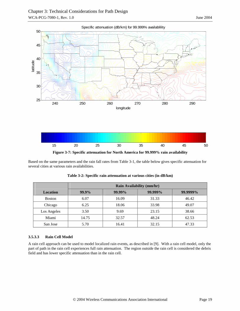
Figure 3-7 below illustrates the specific attenuation in dB/km for North America for 99.999% rain availability. The results are for center frequency of 86 GHz, horizontal polarization, and an elevation angle of 0º.
Chapter 3: Technical Considerations for Path Design WCA-PCG-7080-1, Rev. 1.0 June 2004
© 2004 Wireless Communications Association International Page 19
15 20 25 30 35 40 45 50
240 250 260 270 280 29025
30
35
40
45
50
longitude
latit
ude
Specific attenuation (dB/km) for 99.999% availablility
Figure 3-7: Specific attenuation for North America for 99.999% rain availability
Based on the same parameters and the rain fall rates from Table 3-1, the table below gives specific attenuation for several cities at various rain availabilities.
Table 3-2: Specific rain attenuation at various cities (in dB/km)
Rain Availability (mm/hr)
Location 99.9% 99.99% 99.999% 99.9999%
Boston 6.07 16.09 31.33 46.42
Chicago 6.25 18.06 33.98 49.07
Los Angeles 3.50 9.69 23.15 38.66
Miami 14.75 32.57 48.24 62.53
San Jose 5.70 16.41 32.15 47.33
3.5.3.3 Rain Cell Model
A rain cell approach can be used to model localized rain events, as described in [9]. With a rain cell model, only the part of path in the rain cell experiences full rain attenuation. The region outside the rain cell is considered the debris field and has lower specific attenuation than in the rain cell.

Chapter 3: Technical Considerations for Path Design WCA-PCG-7080-1, Rev. 1.0 June 2004
© 2004 Wireless Communications Association International Page 20
Figure 3-8: Rain cell model
The diameter of the rain cell is a function of the rainfall rate and is given as follows:
km 3.3 08.0−= Rdc (Equation 3-2)
where R is the rainfall rate in mm/hr. Figure 3-9 below illustrates the diameter of rain cell as a function of rain fall rate as outlined in [9]. The size of the rain cell decreases as the rain fall rate increases.
0 50 100 150 200 2502
2.2
2.4
2.6
2.8
3
3.2
3.4
Rain Rate (mm/hr)
Dia
met
er o
f th
e R
ain
Cel
l (km
)
Figure 3-9: Diameter of a rain cell
Within the rain cell, the specific attenuation is defined by (Equation 3-1). The specific attenuation in the debris field decreases as the distance from the center of the rain cell increases. An equation for the attenuation between the edge of the cell and a point outside the rain cell is given in [9]. A more general formulation in terms of the specific attenuation (in dB/km) is derived from the derivative of the debris field attenuation function. The specific attenuation at a distance d (in km) from the center of the rain cell is given as follows:

Chapter 3: Technical Considerations for Path Design WCA-PCG-7080-1, Rev. 1.0 June 2004
© 2004 Wireless Communications Association International Page 21
>
−−
⋅
≤
=Γ
2)cos(
2exp
2
c
m
c
R
cR
dd
r
dd
dd
εγ
γ
(dB/km) (Equation 3-3)
where rm is the scale length for rain attenuation, given by:
19.0)1(5.0 10600 +−−= Rm Rr
and ε is the elevation angle. Figure 3-10 below illustrates the typical specific attenuation versus distance (from center of rain cell) curve for various rain rates.
0 1 2 3 4 5 6 7 8 9 100
5
10
15
20
25
30
35
40
Distance from Center of Rain Cell (km)
Rai
n A
tten
uatio
n (d
B/k
m)
10 mm/hr40 mm/hr80 mm/hr120 mm/hr
Figure 3-10: Rain rate attenuation versus distance from center of a typical rain cell
3.5.3.4 Calculation of Total Attenuation of a Path with Raincell Model
The calculation of total attenuation of a path can be divided into two cases. The first case is where the path is entirely in the rain cell. The second case is where all or part of the path is outside the rain cell.
Case 1: The Path is Entirely in the Rain Cell The size of the rain cell is determined based on the desired rain fall rate with (Equation 3-2). If the path lies entirely with in the rain cell as shown in Figure 3-11, then (Equation 3-1) is used to determine the specific attenuation from the rain fall rate. Multiplying the specific attenuation by the length of the path gives the rain loss for the path.

Chapter 3: Technical Considerations for Path Design WCA-PCG-7080-1, Rev. 1.0 June 2004
© 2004 Wireless Communications Association International Page 22
Figure 3-11: Path entirely in the rain cell
Case 2: Part of the Path is Outside the Rain Cell The size of the rain cell is determined based on the desired rain fall rate with (Equation 3-2). In this case the path (segment AB in Figure 3-12) is divided into two sections. For the part of the path within the rain cell (segment DB in Figure 3-12), the approach in Case #1 is used to determine the rain loss.
For the part of the path outside of the rain cell (segment AD in Figure 3-12), (Equation 3-3) is used to determine the specific attenuation from the rain fall rate. For example, the specific attenuation at point E in Figure 3-12 is calculated based on the distance d between point E and point C (the center of rain). The rain loss along the segment AD can be calculated by integrating the specific attenuation along the path as given in the equation below.
dBin )cos(
2exp
dd
r
dd
RD
A
m
c
RL ∫
−−
⋅=ε
γ
Figure 3-12: Part of the path is outside the rain cell
For paths which are entirely in the debris field outside the rain cell, the path is comparable to segment AD and this same approach is used. Similarly, paths in which the two ends of the link are in the debris field but part of the path passes through the rain cell, can be segmented and this same approach used.

Chapter 3: Technical Considerations for Path Design WCA-PCG-7080-1, Rev. 1.0 June 2004
© 2004 Wireless Communications Association International Page 23
3.5.4 Precipitation Induced Depolarization
Depolarization on atmospheric propagation paths is described in [11]. In this recommendation, the calculation for cross-polarization discrimination (XPD) is outlined for an earth-space telecommunication system in the frequency range of 8 – 35 GHz. The calculation includes a rain dependent term and an ice crystal dependent term. A simplified terrestrial XPD model which excludes the ice crystal dependent term is described in [12]. Further modifications have been made to expand the applicable range of the calculations for higher frequencies based on further measurement data as described in [13].
The equations below calculate the XPD dependence on rain attenuation for frequencies between 71 and 86 GHz. The calculation is based on the modification for higher frequencies in [13] and excludes the ice crystal dependent term as in [12]. Since the only allowable polarization in this band is linear, the equations below are only for linear polarization. The polarization dependent term from the XPD equation in [11] has been fixed to linear. The calculation in [11] also contains a raindrop canting angle distribution term. Since the variation in XPD is very small with respect to raindrop canting angle, the worst case has been used for simplicity.
Equation for calculating XPD [11]:
θCCC Af +−+=15XPD
Frequency dependent term [13]:
35GHzfor )(log26 10 >×= ffC f
f: frequency (GHz)
Rain attenuation dependent term [13]:
35GHz for )(log20 10 >×= fCPACA
CPA: co-polar attenuation (rain attenuation) (dB)
Elevation angle dependent term [11]:
o
o
60for 1.12
60for 180
cos10log40
>
≤
−=θ
θθπθC
θ: path elevation angle (degrees)
Figure 3-13 below illustrates the XPD dependence on rain attenuation for two frequencies, 71 and 86 GHz. The results are given for the worst case elevation angle, 0º.
For the deepest rain fades, the scattering should not reduce the XPD to less than 28 dB, just slightly less than the industry-proposed antenna XPD requirement (assuming a best case rain fade margin of ≈60 dB).
Actual antennas for this band are expected to have a maximum XPD (which will occur in the boresight direction) of no more than 30 to 35 dB. For rain attenuation in the range 0 to ≈30 dB, or for all antenna discrimination angles aside from the boresight direction, the antenna XPD will be less than the atmospheric XPD shown in Figure 3-13. Under any such conditions the reduction in XPD caused by rain is negligible and may be ignored in interference calculations. However, for interference calculations where rain attenuation of more than ≈30 dB is assumed and boresight alignment of both antennas is involved, the reduction in XPD as a result of propagation through the rainy atmosphere should be taken into account. The following examples illustrate these concepts:
Example 1: We are interested in calculating the interference from a vertically polarized transmitter into a horizontally polarized receiver. The interfering antenna, aligned with its mainbeam towards the victim receiver, has discrimination values of 0 dB on the VV pattern and 35 dB on the VH pattern. The victim antenna, aligned with its mainbeam towards the interfering transmitter, has discrimination values of 0 dB on the HH pattern and 33 dB on the HV pattern. The total crosspolar discrimination for V into H in clear air is the lesser of (VV of the interfering antenna plus HV of the victim antenna) or (VH of the interfering antenna plus HH of the victim antenna). Thus interference analysis in clear air would assume total V into H discrimination of 33 dB. However, interference calculations done under the assumption of 60 dB rain fade of the desired signal should only assume total

Chapter 3: Technical Considerations for Path Design WCA-PCG-7080-1, Rev. 1.0 June 2004
© 2004 Wireless Communications Association International Page 24
discrimination of 28 dB as shown in Figure 3-13.1
0 10 20 30 40 50 60 70 80 90 10020
25
30
35
40
45
50
55
60
65
70
Rain attenuation (dB)
Cro
ss P
olar
izat
ion
Dis
crim
inat
ion
(dB
c)
Elevation angle = 0o; Linear Polarization
Freq = 71GHzFreq = 86 GHz
Figure 3-13: Atmospheric induced depolarization
Table 3-3: Discrimination Combinations for Example 1
Interfering AntennaRainy
Atmosphere Victim Antenna Total Worst Case Value
PatternDiscrimination (dB) Pattern
Discrimination (dB) TX -->RX
Discrimination (dB) TX -->RX
Total Discrimination (dB)
VV 0 Co-pol 0 HV 33 VH 33VV 0 X-pol 28 HH 0 VH 28VH 35 Co-pol 0 HH 0 VH 35VH 35 X-pol 28 HV 33 VH 96
VH 28
Example 2: We are interested in calculating the interference from a vertically polarized transmitter into a horizontally polarized receiver. The interfering antenna, aligned with its mainbeam towards the victim receiver, has discrimination values of 0 dB on the VV pattern and 35 dB on the VH pattern. The victim antenna, aligned with its mainbeam 5° from the interfering transmitter, has discrimination values of 35 dB on the HH pattern, 45 dB on the HV pattern, 35 dB on the VV pattern, and 45 dB on the VH pattern. The total crosspolar discrimination for V into H in clear air is the lesser of (VV of the interfering antenna plus HV of the victim antenna) or (VH of the interfering antenna plus HH of the victim antenna). Thus interference analysis in clear air would assume total V into H discrimination of 45 dB. The total co-polar discrimination for V into V in clear air is the lesser of (VV of the interfering antenna plus VV of the victim antenna) or (VH of the interfering antenna plus VH of the victim antenna). Thus interference analysis in clear air would assume total V into V discrimination of 35 dB. The total crosspolar discrimination is only 10 dB greater than the total discrimination for the co-polarized case, and the maximum potential reduction of XPD to 28 dB for up to 60 dB of rain fade shown in Figure 3-13 is negligible.
1 Strictly speaking the contribution of each combination should be added so that the total discrimination would be 26.2 dB here. However, by industry convention, path/frequency coordination calculations typically take the lowest value alone, and we propose to continue this convention for the 71-86 GHz band.

Chapter 3: Technical Considerations for Path Design WCA-PCG-7080-1, Rev. 1.0 June 2004
© 2004 Wireless Communications Association International Page 25
Table 3-4: Discrimination Combinations for Example 2
Interfering AntennaRainy
Atmosphere Victim Antenna Total Worst Case Value
PatternDiscrimination (dB) Pattern
Discrimination (dB) TX -->RX
Discrimination (dB) TX -->RX
Total Discrimination (dB)
VV 0 Co-pol 0 VV 35 VV 35VV 0 X-pol 28 VH 45 VV 73VH 35 Co-pol 0 VH 45 VV 80VH 35 X-pol 28 VV 35 VV 98
VV 0 Co-pol 0 HV 45 VH 45VV 0 X-pol 28 HH 35 VH 63VH 35 Co-pol 0 HH 35 VH 70VH 35 X-pol 28 HV 45 VH 108
VV 35
VH 45
3.5.5 Fog Loss
The calculation for attenuation due to clouds and fog is outlined in [14]. The figure below illustrates the specific attenuation due to fog for a temperature of 15ºC over the range of frequencies from 71-86 GHz.
72 74 76 78 80 82 84 860
0.2
0.4
0.6
0.8
1
1.2
1.4
1.6
1.8
2
Frequency (GHz)
Spe
cific
Att
enua
tion
(dB
/km
)
Temperature = 15oC
Medium FogThick Fog
Figure 3-14: Specific attenuation due to fog
As shown in the figure above, even in thick fog at 86 GHz the attenuation due to fog is less than 2dB/km. This is significantly less than rain attenuation in these frequency bands and therefore attenuation due to fog can be ignored in the path loss calculation. In addition, for terrestrial line-of-sight links attenuation due to clouds can be ignored.
3.5.6 Snow and Ice Loss
In the lower millimeter wave bands, measurements have shown attenuation due to snow and ice one to two orders of magnitude lower than that of rain at similar effective precipitation rates [15]. Based on these measurements, we assume that the same holds true for E-band; further research, however, is required. Rain attenuation will therefore dominate and this propagation loss will be considered negligible for the purposes of availability calculations.

Chapter 3: Technical Considerations for Path Design WCA-PCG-7080-1, Rev. 1.0 June 2004
© 2004 Wireless Communications Association International Page 26
3.5.7 RF Backscatter Due to Precipitation
Backscattered radiation from rain can cause self-interference or near-neighbor interference in a co-sited network geometry. The magnitude of the rain backscatter is considered first in the monostatic case for co-sited geometries, and then in a more general bistatic case. The bistatic case is representative of scenarios in which transmitters are located either on the same rooftop or on different rooftops that are separated by a short distance, say up to 600m. As described in Section 2.3.4, the effects of rain backscatter may cause receiver de-sensitization in bucking scenarios where the signal from a powerful transmitter is reflected into a nearby co-channel receiver. Note that the effects of rain backscatter can be minimized via a harmonized frequency plan.
Co-Sited Backscatter The detailed calculations for rain backscatter are provided in Section D.1 of Appendix D. The results of the analysis are plotted in Figure 3-15. Taking into account the additional propagation loss to rainfall attenuation, the backscatter return flattens out slightly for higher rain rates as shown in the figure.
A transceiver may require up to 115 dB of transmit/receive isolation; much more isolation than rain backscatter will allow. This example isolation requirement derives from a transmitter employing +35 dBm of output power with a sensitivity of -60 dBm and a T/I requirement of 20dB. Automatic Transmitter Power Control is irrelevant in this situation since transmitters will tend to operate at maximum power during strong rain events. Cross-polarizing the receive channel relative to the transmitter in principle provides additional isolation (rain induced depolarization is negligible for the short reflection paths making up most of the backscatter contribution), but still does not allow for clustering transceiver nodes on a rooftop. Dual-band frequency-division duplexing can eliminate this self-interference problem for a single transceiver; co-sited backscatter interference can likewise be eliminated by using harmonized FDD via a coordinated band plan.
Rain Backscatter
-75.00
-70.00
-65.00
-60.00
-55.00
-50.00
0.1 1 10 100 1000
Rain Rate (mm/hr)
Bac
ksca
tter
Po
wer
Rat
io (
dB
)
Backscatter Ratio (73.5 GHz)
Backscatter Ratio (83.5 GHz)
w/ attenuation (73.5 GHz, 2 ft. dish)
w/ attenuation (83.5 GHz, 2 ft. dish)
Figure 3-15: Rain backscatter, power relative to transmitted power
Near-Sited Backscatter The bistatic rain-scattered interference geometry is shown in Figure D-2. Detailed calculations for rain backscatter for the bistatic case are provided in Section D.2 of Appendix D. For this calculation, the scattering cross-section is

Chapter 3: Technical Considerations for Path Design WCA-PCG-7080-1, Rev. 1.0 June 2004
© 2004 Wireless Communications Association International Page 27
assumed constant with angle; this should be true for angles of a few tens of degrees, but may be overly conservative at larger angles.
An accommodation must also be added to the scattered power calculation to account for signal power attenuation in rain; i.e. secondary scattering events. In heavy rain the depth of the effective scattering volume can be determined not only by the geometrical factors but by the signal attenuation as well. In the example shown in Figure 3-16, the 80 dB isolation predicted between two dishes separated by 100m and 10° is insufficient by itself (by 36 dB) to clear a worst-case interfering transmitter with +35 dBm transmit power and receiver with an interference threshold at -81 dBm. However, at 42 mm/hr, signal attenuation due to rain is 16 dB/km, and the scattering volume is about 560m away, so the two-way path signal attenuation is 18 dB. Another 18 dB of isolation is required, which may be realized if elevation differences between beams limit the overlap, and thus the interfering power level in the peak scattering volume. A difference of only 1.2° in elevation will add 22 dB or more of isolation in this case (following recommended FCC radiation pattern envelope restrictions). If scattered radiation cannot be cleared by these means, beam cross-polarization or a harmonized frequency plan may be required.
Figure 3-16: Rain backscatter for bistatic case as a function of separation distance and pointing angle
3.5.8 Over-the-Horizon Loss
The National Spectrum Managers Association (NSMA) has developed a comprehensive over-the-horizon (OH) loss model to calculate path loss for paths that are blocked by terrain or other obstacles [16]. This model generally follows the Longley-Rice approach of Tech Note 101 [17] and implements diffraction from single and multiple knife edges and rounded obstacles as well as troposcattering. The OH loss calculations are based on a profile of the path in question generated from a database of digitized terrain. The profile may also include above-ground obstacles where information about these is available. Although the general approach of the NSMA model is applicable to 71-76 and 81-86 GHz, only the single-knife-edge diffraction portion is expected to work correctly in these bands. The use of the single knife-edge model is recommended initially with the understanding that this model will under-predict the actual OH loss for a conservative approach. In other words, it is expected that actual measured OH loss will be much greater than predicted by this model further reducing a potential interfering signal. Further work is needed on this model with respect to how the loss is calculated for each of the modes and how the choice is made of which mode is controlling for a particular path profile. It is expected that the necessary modifications to the OH loss model can be specified in a future revision of this document.
It is expected that the primary use of OH loss in the 71-76 and 81-86 GHz bands would be to show non-interference to observatories in the radio astronomy service (RAS). These observatories may be quite sensitive to external interference and may therefore require large coordination distances if line-of-sight propagation is assumed. The
)(dBP
P
t
v
θi (degrees)
R = 42 mm/hr G = 50 dBi No rain attenuation σ(θ) = σ(0)
d =100 m
d =200 m
d =400 m

Chapter 3: Technical Considerations for Path Design WCA-PCG-7080-1, Rev. 1.0 June 2004
© 2004 Wireless Communications Association International Page 28
effect of terrain blockage as calculated by the OH loss model may be used to reduce the necessary coordination distance of a proposed fixed-service transmitter.
OH loss may also be used to enhance coordination among terrestrial fixed-service millimeter-wave paths. Based on the EIRP levels that are expected to be used initially in these bands, the length of potential paths of interference will be short enough that OH loss will not often come into play – the shorter the interference path, the less likely it is to be blocked by the intervening terrain. However, with increasing EIRP levels in the future, the length of potential paths of interference will increase, and OH loss will become a more important tool to resolve the interference potential.
3.5.9 Building Obstruction Loss
When diffraction over buildings may produce additional loss on a path of potential interference, the OH loss calculations may be used to quantify the loss. The locations and heights of buildings that would produce such blockage may be identified from site surveys or may be retrieved from accurate GIS building databases, when available.
For diffraction around the sides of buildings or other blockage situations, such as an antenna located inside a building and directed out a window, the OH loss model may not be a valid way to quantify the amount of additional path loss. In these situations, the path coordinator may make qualitative judgments that the blockage is or is not sufficient to mitigate a potential interference case. Of course, resolution of cases in this manner is subject to the condition that the later-coordinated system is always responsible for correcting any actual harmful interference that occurs. To facilitate consideration of shielding blockage in the coordination process, path registrants are expected to provide an accurate description of the location of the antennas (e.g. “10 Main Street, shooting out a 12th floor window, north side”).
3.6 Building and Tower Sway
3.6.1 Building Sway
Minimizing the motion of tall buildings has always been a design requirement to preclude adverse health effects on inhabitants. Early tall buildings were designed to be stiff to resist sway due to high wind; modern tall buildings incorporate dampers to counteract the effects of wind. For example, the John Hancock Tower in Boston uses a huge block of concrete floating in a bed of oil, positioned by computer-controlled hydraulics to offset building sway. Sydney's Chifley Tower utilizes a giant block of concrete hanging by wires. Taipei 101 uses an 18-ft. diameter, 800-ton sphere that swings like a pendulum from the 92nd floor. Water tanks on the roofs of tall buildings, necessary to ensure sufficient water pressure, are sometimes engineered to also serve as wind dampers.
Based on measurements made in tall buildings over 30 stories in downtown Seattle [18], the following observations were made:
• Of thirty-five buildings tested, thirteen exhibited sway (from moderate to high wind) > ± 0.03° during about 10 hours per year.
• It is impossible to predict actual sway behavior of a building based solely on observation (detailed construction details, and wind intensity and paths as influenced by surrounding structures is necessary).
Based on measurements made in buildings less than 30 stories high, in downtown Seattle [18], the following observations were made:
• Of eleven buildings tested, none exhibited sway (from moderate to high wind) of > ± 0.03°.
• It is impossible to predict actual sway behavior of a building based solely on observation (detailed construction details, and wind intensity and paths as influenced by surrounding structures is necessary).

Chapter 3: Technical Considerations for Path Design WCA-PCG-7080-1, Rev. 1.0 June 2004
© 2004 Wireless Communications Association International Page 29
3.6.2 Tower Sway
In general, each individual tower is custom designed for its particular site, intended use and antenna load. Design considerations include: soil type and size of the building lot, environmental impact due to tower shape, cellular or microwave use (which sets limits on allowable bending, swaying, and twisting), number, size, weight, type, and orientation of antennas (which affects static and dynamic loading), wind/ice loading, etc.
There are two basic types of towers: guy- and self-supporting. Guyed towers are relatively slender structures that are supported by cables anchored to the ground (see Figure 3-17a). Guyed towers cost the least of any tower type since the structure requires the least metal; however, a very large building lot is required for locating the guy cable anchors (at a distance from the base as much as 80% of the tower height). Guyed towers can be designed to accommodate the full range of loading from light-duty microwave, cellular, and land mobile radio antennas, to heavy-duty microwave, broadcast, and cable television.
• An existing guyed tower may have sufficient stability for a 0.5° beamwidth E-band antenna if the tower was generously over designed and intended for supporting point-to-point microwave antennas (which generally have beamwidths of about 2°). Mount the E-band antenna as low as possible on the tower.
• Existing guyed towers supporting only cellular or mobile radio antennas (which generally have beamwidths >15°) are probably unsuitable for 0.5° beamwidth E-band antennas: expected tower movement would be very high.
Self-supporting towers are generally available as either monopoles or three- or four-legged, lattice-braced, tapered “boxes” (see Figure 3-17b and c). Monopoles have cross-sections that are usually tubular or tapered along the pole length. Both types of monopoles are intended for relatively light loads and they sway, bend and twist appreciably. However, their low cost (especially considering the small lot size that is required) makes the monopole attractive for cellular applications because of the broad beamwidth of cellular antennas. Most manufacturers rate the sway and bend limits of their monopoles at 3 degrees at the top of the pole for 50 MPH winds. Note that the tapered monopole bends much more at the top than near the base, and that near the base the actual swaying and bending will generally be significantly less than the 3 degree specification.
• It is unlikely that any existing monopole has sufficient stability for supporting a 0.5° beamwidth E-band antenna.
• If an attempt is necessary (i.e. there are no alternatives), mount the E-band antenna as low as possible.
The three- or four- legged, lattice-braced, tapered “box” tower can be designed to accommodate the full range of loading from light to very heavy duty, and is a popular design for towers that include microwave antennas.
• Among existing towers, the three- or four-legged, lattice-braced, tapered “box” tower is probably the most likely to successfully support an E-band antenna installation, especially if the tower is currently supporting point-to-point microwave antennas. Existing towers supporting only cellular or mobile radio antennas are probably unsuitable.
• Mount the E-band antenna as low as possible on the tower.
Figure 3-17: Types of Towers
Guyed towers can θ top The three-legged,
be designed for Since θ top>>θ bot self-supporting
relatively high wind, for a tapered tower can be
freedom from monopole, there is designed for
bending, less bending, sway, relatively high
sway, or θ bot or twist near its freedom from
twist. base. bending, sway,
or twist. (a) Guyed Tower (b) Tapered Monopole (c) Three-legged Self-Supporting

Chapter 3: Technical Considerations for Path Design WCA-PCG-7080-1, Rev. 1.0 June 2004
© 2004 Wireless Communications Association International Page 30
3.7 Antenna RPE Smearing Due to Geographic Coordinate Inaccuracy The position of the transmitters at the two ends of a link will dictate the pointing direction of their antennas. However, if the actual position of the transmitters is different than that reported to the path coordinator, the true pointing angle of the antennas will be different than that calculated by the path coordinator. In such a case, the interference environment will not be accounted for properly. Therefore, uncertainty in the position of the transmitter due to the error in the position measurement must be accounted for in the path coordination interference calculation.
Figure 3-18 below illustrates the reported position of transmitters at two ends of a link. Also illustrated is the possible area in which the transmitters (A & B) could actually be located based on position measurement error. Though exaggerated by the figure, one can see that the path of the link based on the reported position can be different than the actual link. In one possible path, transmitter A could be located in the bottom right hand corner of the error box and receiver B is located in the upper left hand corner of the error box. In this case, the antenna of transmitter A will be oriented such that it is pointed directly at receiver C and will cause much more interference than expected.
Figure 3-18: Diagram illustrating position error
In order to keep positioning error within reasonable bounds, the following are the recommended accuracies for coordinate measurements2:
• For transmitters with >40dBW EIRP, horizontal accuracy of ±1m, vertical accuracy, ±5m
• For transmitters with <40dBW EIRP, horizontal accuracy of ±3m, vertical accuracy±15m
In the case of a 3-meter GPS measurement error on each end the link, the total worst case error will be 6 meters. For a path length of 500 meters, the worst case pointing offset from reported would be 0.7º. This error is comparable to the half power beamwidth of an antenna in this frequency band, thus requiring this effect to be accounted for in the path coordination process.
The maximum amount of pointing offset between the two ends of a link is calculated as follows.
2 and 1location between length path :D
2location at error t measuremenposition :
1location at error t measuremenposition :
degreesin 180
tan
2
1
21
21
p
p
ppD
pp
⋅
−−+
=π
θ
The manner in which the position measurement error is incorporated into the interference calculation is to expand the boresight of the antenna pattern in the interference calculations by the maximum amount of pointing offset in positive and negative angles off boresight.
2 Note that WAAS-enabled GPS receivers are typically capable of ±3m horizontal measurement accuracy.

Chapter 3: Technical Considerations for Path Design WCA-PCG-7080-1, Rev. 1.0 June 2004
© 2004 Wireless Communications Association International Page 31
>−≤
=θψθψθψ
ψfor )(
for )0()(
g
ggm
where )(ψg is the gain of the normal antenna pattern and ψ is the angle off boresight.
Figure 3-19 below illustrates the modification of an example antenna pattern by stretching the boresight of the antenna. The example is for a 0.8º half power beamwidth antenna with a 5º pointing offset (an exaggerated pointing error to more clearly illustrate the effect).
-15 -10 -5 0 5 10 1510
15
20
25
30
35
40
45
50
Angle off Boresight (degrees)
Ant
enna
Gai
n (d
Bi)
Example antenna pattern
Normal antenna patternModified antenna pattern
Figure 3-19: Antenna pattern modified by pointing offset
3.8 Recommended ATPC Behavior Historically, the ATPC guidelines of TSB-10F have limited the coordination advantage to 10 dB in an environment where the link fade margins are typically 30 dB or greater. Thus if a transmitter operates at its maximum ATPC power for a given period of time, it does not directly cause an outage of nearby receivers.
In contrast, the proposed ATPC operation in the 70/80 GHz bands uses a much greater range of power adjustment and greater coordination advantage. Based on the assumption that fading of the desired and interfering signal paths will be closely correlated under rain fading conditions, only a relatively small margin may be considered necessary between the actual C/I produced by interfering links and the critical C/N of the receiver. In this environment, should a transmitter increase its power other than in response to rain fading it could directly cause an outage of nearby receivers. Examples of path conditions that could cause such an ATPC power increase are path obstruction, an antenna becoming misaligned, and equipment malfunctions. The following ATPC requirements for the 70/80 GHz bands are proposed to3:
• Limit the potential impact of ATPC activity on nearby links.
3 Although we have proposed a conservative approach to ATPC (i.e., C/N-based adaptation), we recognize that a C/I+N-based approach may have superior performance. However, further studies supported by measured data on network stability of C/I+N-based approaches should be performed prior to adopting this alternative.

Chapter 3: Technical Considerations for Path Design WCA-PCG-7080-1, Rev. 1.0 June 2004
© 2004 Wireless Communications Association International Page 32
• Allow ATPC to protect against rain outage while forcing corrective action in response to other path problems.
• Decouple ATPC activity among paths in an area by eliminating power increases in response to increased interference alone.
ATPC Guidelines for the 70/80 GHz Bands:
1. The minimum ATPC dynamic range requirements and ATPC adaptation rule as follows are recommended:
a. Minimum ATPC dynamic range = maximum(0, EIRPdBW – 23); note this means that transmitters whose maximum output EIRP is <23 dBW need not employ ATPC.
b. The ATPC function shall set the C/N at the receiver to <T+10 dB, where T is the static threshold of the receiver, or
c. Reduce the transmitter’s output power to the specified minimum (e.g., this situation occurs over a short link range in clear air).
2. The ATPC system shall only increase the transmitter power in response to path fading as identified by a decrease in received signal level (RSL). The ATPC system shall not increase the transmitter power in response to measurement of a degraded BER.
3. The ATPC system shall implement a feedback loop such that the RSL measurements control increases in the power of the associated transmitter at the other end of the link. The ATPC system shall not increase the transmitter power in response to measurement of a decreased RSL at the local receiver alone.
4. Fading greater than 10 dB with respect to the installed RSL (clear air installation assumed) and the associated ATPC activity shall be recorded to allow an operator to either confirm that the fading activity is caused by precipitation or otherwise to troubleshoot the link. This alarm is a warning only and may automatically reset itself when the RSL returns to a normal level.
5. If a usable signal (e.g., defined by BER>10-6 or other metric) is not received for a period of 5 minutes, the ATPC system shall return the transmitter power to its minimum level and trigger an alarm. After this, the transmitter should power up for no more than 1 second every 30 seconds to determine if the link can be re-established.

Chapter 4: Terrestrial Service Path Coordination Process WCA-PCG-7080-1, Rev. 1.0 June 2004
© 2004 Wireless Communications Association International Page 33
4 Terrestrial Service Path Coordination Process
A technically sound and efficient path coordination process has been successful in the lower terrestrial microwave bands for many years. This section recommends guidelines and procedures to implement a similar process adapted to the properties of the E-band while allowing for the implementation of more efficient, automated processes such as web-based link registration, centralized or shared data sets, and near real-time interference analysis results.
4.1 Link Registration Parameters The parameters required to register a new link are categorized into either Administrative and Geographic information or Antenna and Radio Equipment data. Geographic parameters include site coordinates, ground elevation, site name, etc., while the administrative data identifies the licensee, station class, call sign, etc. Equipment parameters consist of radio and antenna types and their associated specifications.
4.1.1 Measurement and Input of Site Coordinates
Obtaining accurate site coordinates for the desired link is critical to a meaningful interference analysis against other operational or planned links due to the short path distances anticipated for this band. Site coordinates are to be either measured with a GPS device or obtained by professional site survey methods. It is important to obtain site coordinates at the intended location of the transmitting antenna. Subsequent changes to the intended antenna location should be re-measured to obtain accurate coordinates, even on the same building rooftop. All coordinates should be given in NAD83 and reported to the hundredths of a second in latitude / longitude.
4.1.2 Administrative and Geographic Parameters
The following table details the administrative and geographic parameters to be submitted for each end of a particular link.
Table 4-1: Administrative & Geographic Parameters
Data Field Units / Type Example
Site Name High Peak
Latitude DD-MM-SS.ss N/S 35-43-22.53 N
Longitude DDD-MM-SS.ss E/W 081-36-29.32 W
Ground Elevation m - AMSL 658.37
Antenna Location Detailed Description
“10 Main Street, shooting out a 12th floor window, north side”
Call Sign WIA422
Licensee Virginia Energy
Station Class FXO
Link Status Proposed
Link ID VE00001

Chapter 4: Terrestrial Service Path Coordination Process WCA-PCG-7080-1, Rev. 1.0 June 2004
© 2004 Wireless Communications Association International Page 34
Data Field Units / Type Example
Registration Date 01/22/04
Registration Time hh-mm-ss 13-04-12 UTC
4.1.3 Antenna and Radio Equipment Parameters
The following table identifies the required antenna and radio equipment parameters for each transmitting or receiving unit at each end of the link.
Table 4-2: Antenna and Radio Equipment Parameters
Data Field Units / Type Example
Antenna Manufacturer Andrew
Antenna Model HP-7080A
Antenna Gain dBi 50.0
Antenna Beamwidth degrees 0.6
Antenna Centerline m - AMSL 52.43
Radio Manufacturer Cisco
Radio Model 4800 GE
Modulation BPSK
Stability % 0.01
Transmit Power4 (min / max) dBm 5.0 / 25.0
Emission Designator 1G25D7W
Emission Bandwidth GHz 1.25
Number of Channels 2
Channel Center Frequencies GHz 73, 75, 83, 85
Receiver Threshold dBm -70.0
Fixed Loss dB 3.0
4.1.4 Other Parameters Obtained from Radio and Antenna Vendor
In addition to the basic descriptions and specifications identified above, antenna vendors must provide radiation pattern envelopes that characterize the antenna performance in all azimuth directions for each polarity combination. An example for RPE data is shown in Figure 4-1.
4 The difference between minimum and maximum transmitter power represents the ATPC range of the transmitter

Chapter 4: Terrestrial Service Path Coordination Process WCA-PCG-7080-1, Rev. 1.0 June 2004
© 2004 Wireless Communications Association International Page 35
Figure 4-1: Sample antenna data
The radio vendor must provide T/I values for their equipment for all pertinent frequency separations; an example is shown in Figure 4-2 (refer also to Appendix B).
Figure 4-2: Sample T/I curve data

Chapter 4: Terrestrial Service Path Coordination Process WCA-PCG-7080-1, Rev. 1.0 June 2004
© 2004 Wireless Communications Association International Page 36
4.1.5 Parameters Supplied by Path Coordinator
The path coordinator provides (through data inputs and calculations) all of the associated parameters needed to determine the various interference conditions with other links in the band. These parameters include distances, bearings, discrimination angles, T/I objectives, calculated interference levels, etc. These values determine specific interference case predictions and allow the licensee to determine their link viability based on the environment link registration database. Once the proposed link has been shown to not cause harmful interference to incumbent links, the parameters shown in Table 4-3 are provided for each end of the link.
In addition, while the basic parameters for links are supplied by the licensee and equipment vendors, the path coordinator typically is charged with maintaining the data sets and updating as needed. For example, when a new radio is certified the path coordinator will typically enter all necessary specifications for the radio into the appropriate data tables. Values for ATPC range, T/I curves, receiver threshold, etc. are updated or entered for use in the appropriate interference analysis. Licensees are encouraged to help obtain new equipment information from the vendors as needed.
Table 4-3: Parameters supplied by the Path Coordinator
Data Field Units / Type Example
Latitude5 DD-MM-SS.ss N/S 35-43-22.53 N
Longitude DDD-MM-SS.ss E/W 081-36-29.32 W
Transmit Power (maximum)6 dBm 20.0
Transmit Frequency GHz 72.25
Polarization V or H V
4.2 Engineering Analysis An interference analysis against a database of registered links is required to determine whether frequencies and polarizations may be assigned to a proposed new link. The proposed link passes the frequency coordination process if it can be determined not to cause harmful interference to or receive harmful interference from any previously registered links.
4.2.1 Objective of the Analysis
We recommend that the interference objectives for these bands should be defined as follows:
For receivers employing digital modulation: based upon manufacturer data and following the procedures in this Guide, for each potential case of interference a threshold-to-interference ratio (T/I) shall be determined that would cause 1.0 dB of degradation to the static threshold of the protected receiver. For the range of carrier power levels (C) between the clear-air (unfaded) value and the fully-faded static threshold value, in no case shall interference cause C/I to be less than the T/I so determined unless it can be shown that the availability of the affected receiver would still be acceptable despite the interference.
Harmful interference should therefore be defined as interference that causes C/I < T/I for any carrier power level C between the clear-air (unfaded) value and the fully-faded static threshold value, and that also unacceptably degrades the reliability of the affected link. 5 The latitude and longitude are included here to identify the endpoint to which the other parameters apply. 6 Note that the coordinated transmit power may be less than the output power capability of the equipment.

Chapter 4: Terrestrial Service Path Coordination Process WCA-PCG-7080-1, Rev. 1.0 June 2004
© 2004 Wireless Communications Association International Page 37
Because of the short path lengths that must be used to ensure highly reliable communications, the sole cause of deep fading in these bands is rain attenuation. Rain fading is often highly correlated among links in an area, meaning that interfering signals may, to some degree depending on the geometry of the links, fade along with the desired signal. By stating the interference objectives this way we can take advantage of the correlated rain fading to enhance the coordination possibilities. This is illustrated graphically in Figure 4-3.
Figure 4-3: Interference objective
4.2.2 Interference Cases to be Analyzed Between Paths
Between a proposed link A-B and an environment link C-D there are, in general, eight potential interference cases that need to be resolved to say that A-B does not have interference with C-D. These cases are A into C, A into D, B into C, B into D, C into A, C into B, D into A, and D into B. In the subsequent discussion it should be understood that all of these cases must be analyzed for every pair of proposed and environment links.
Depending on the duplexing architecture of the links (e.g. FDD or TDD) and the frequency segments used, some of the eight combinations may naturally drop out. For example, if both the proposed and environment links use a dual-band FDD architecture by transmitting in one band segment (71-76 or 81-86 GHz) and receiving in the opposite segment, then the analysis is simplified because four of the above cases are automatically resolved based on sufficient frequency separation. The receivers of the dual-band FDD radios must be able to operate without having interference from their own transmitters, and therefore we can safely assume that there will always be sufficient filtering on these radios so that “high into low” (81-86 GHz into 71-76 GHz) interference, or vice versa, will not occur.
As a result of variation in rain rates within rain cells, and formation and movement of rain cells, there is a possibility that interference paths and desired paths may be instantaneously exposed to different fading conditions despite the following analysis procedure. The desired path fading could instantaneously be greater than the interference path resulting in a short-time violation of the interference objective criteria. The result would be additional seconds of unavailability of the victim receiver. We believe that this differential fading will only occur for small percentages of time that are negligible with respect to the link availability budgets; however, our approach is subject to verification by simulation or field data.
Carrier Level
Interference Limit
Clear Air
Threshold
Sig
nal
Lev
el (
dB
m)
T/I
Rain Attenuation of the Desired Signal (dB)

Chapter 4: Terrestrial Service Path Coordination Process WCA-PCG-7080-1, Rev. 1.0 June 2004
© 2004 Wireless Communications Association International Page 38
4.2.3 Analysis Steps to Demonstrate Non-Interference
The following steps are the recommended approach to interference analysis. The steps move generally from least to most computationally complex and from least to most aggressive in terms of assumptions about correlation of rain fading between the desired and interfering signal paths. By following these steps it is anticipated that nearly all interference cases may be cleared with a simple distance search or with a basic C/I calculation. It is hoped that only a small number of cases are likely to require more detailed calculations taking into account the correlated rain fading. The steps in the interference analysis are:
1. Get feedback from the NTIA site for Federal Government Links (cf. Section 4.4.2) and RAS observatories (cf. Section 5) to ensure the proposed sites will not interfere with these entities.
2. Define a circular coordination zone as described in Section 4.2.3.1 and collect the set of all potentially affected links.
3. For each proposed transmitter, calculate the interference into each registered receiver in the area that uses the same band segment (e.g. 71-76 GHz or 81-86 GHz). Likewise calculate the interference from each registered transmitter in the area into each proposed receiver. These are clear-air calculations but may include the atmospheric absorption loss of the area, nominally 0.4 dB/km. Cases that show interference 6 dB below the receiver thermal noise power or lower, including the effect of any receiver filtering, may be considered resolved and eliminated from further consideration. These calculations are based on the worst-case (and generally unrealistic) assumption that the desired signal is fully rain-faded, but the interfering signal has no rain fading whatsoever. Many links will be able to be cleared with this relatively simple screen. The details of this step are described in Section 4.2.3.2. These calculations will take into account the specific T/I requirements of the receivers.
4. For the cases remaining after step 3, consider the link geometry and apply the appropriate geometric rules of thumb as described in Section 4.2.3.3.1 through Section 4.2.3.3.3. As noted above, these screens are in increasing level of computational complexity and increasing level of assumption on the degree of rain-fading correlation between the desired and interfering paths. Most of the links should be cleared after this step. These calculations will take into account the specific T/I requirements of the receivers.
5. For all remaining cases, the final step is to use the rain cell model to determine if clearing the interference is possible. This is described in Section 4.2.3.4 and basically involves placing a simulated rain cell over a carefully selected set of geographic grid locations and varying the rain rate over the full range of expected rain rates to determine whether interference will occur. These calculations will take into account the specific T/I requirements of the receivers.
6. If the proposed link still cannot be cleared, additional mitigation options may be considered. These may be undertaken at the discretion of the path coordinator and may require additional fees:
• Cross polarization • Terrain/Building/Clutter Blockage (OH Loss) • Vertical antenna discrimination for boresight cases in the azimuth plane • Relocating the antenna
7. Get feedback from the FCC when links are deployed in US border areas and could possibly interfere with links in Canada or Mexico (cf. Section 4.6).
8. If any cases cannot be satisfactorily resolved, the link may not be registered.
4.2.3.1 Step #1: Circular Coordination Contour / Radius Search
Links from the database that are within a radius of the proposed new link should be considered for possible interference while those beyond this radius may be eliminated. A search radius of 100 km around the midpoint of the proposed link is considered adequate to include all necessary environment paths. Note that only GPS coordinates are required for this step.
Although with the highest allowable EIRP (85 dBm), with boresight-to-boresight coupling of large antennas, and under line-of-sight propagation conditions, interference is theoretically possible beyond 100 km, the occurrence of such a case is considered highly unlikely. Such a case would require both exact boresight-to-boresight alignment of antennas with very narrow beams and also that the long path of interference not be blocked by terrain. It is felt that the likelihood of such a situation is negligible for path coordination purposes.

Chapter 4: Terrestrial Service Path Coordination Process WCA-PCG-7080-1, Rev. 1.0 June 2004
© 2004 Wireless Communications Association International Page 39
4.2.3.2 Step #2: Assume Fading is Entirely Uncorrelated Among Paths
Under the worst-case assumption that when the desired signal fades to the static threshold, the interference signal does not fade at all, we can show non-interference by requiring the interfering signal to be T/I below the receiver threshold:
( ) quiredStaticActual ITTI Re/−≤
For all of the possible interference cases between the proposed path and the environment paths within the search radius of Step #1 above, calculate the interference level based on the actual parameters of the links and using the maximum ATPC power of the interfering transmitter. Eliminate (resolve) the cases that satisfy the above equation and keep for further analysis the cases that do not.
Example 3: Table 4-4 shows typical parameters for boresight co-polarized interference from a 60 dBm ATPC-equipped transmitter into a similar receiver, and Table 4-5 shows the distances that are necessary to avoid interference as a function of the discrimination angle, FCC required RPE assuming line-of-sight propagation with absorption loss of 0.4 dB/km.
Table 4-4: Parameters for Example 3
Case ParametersInterfering Transmitter Power (dBm) 10
Interfering TX Antenna Mainbeam Gain (dBi) 50Interfering TX EIRP (dBm) 60
Interfering TX Maximum ATPC Power Reduction (dB) 7Interfering TX Antenna Discrimination Angle (deg) 0
Interfering TX Antenna Discrimination (dB) 0Victim RX Bandwidth (MHz) 1000Victim RX Noise Figure (dB) 8
Victim RX Thermal Noise Power (dBm) -76Interference Objective for 1 dB Threshold Degradation (dBm) -82
Victim RX Antenna Mainbeam Gain (dBi) 50Atmospheric Absorption Loss (dB/km) 0.4
Desired Path Length (km) 2Desired Path Loss (dB) 136.7
Desired Transmitter Power (dBm) 10Desired TX Antenna Mainbeam Gain (dBi) 50
Desired TX EIRP (dBm) 60Carrier Level (dBm) -26.68
Victim RX C/N @ 10^-6 BER (dB) 14Victim RX T/I (dB) 20
Victim RX Threshold @ 10^-6 BER (dBm) -62Victim RX Fade Margin (dB) 35.32

Chapter 4: Terrestrial Service Path Coordination Process WCA-PCG-7080-1, Rev. 1.0 June 2004
© 2004 Wireless Communications Association International Page 40
Table 4-5: Required Coordination Distances for Example 3
Victim RX Antenna Discrimination Angle (deg)
Victim RX Antenna Discrimination (dB)
Required Path Loss (dB)
Coordination Distance (km)
Interference Criteria
-180.0 55 137.00 1.900 I<T-(T/I)-30.0 55 137.00 1.900 I<T-(T/I)-29.9 50 142.00 3.200 I<T-(T/I)-20.0 50 142.00 3.200 I<T-(T/I)-19.9 45 147.00 5.300 I<T-(T/I)-15.0 45 147.00 5.300 I<T-(T/I)-14.9 40 152.00 8.200 I<T-(T/I)-10.0 40 152.00 8.200 I<T-(T/I)-9.9 36 156.00 11.300 I<T-(T/I)-5.0 36 156.00 11.300 I<T-(T/I)-4.9 0 192.00 63.800 I<T-(T/I)0.0 0 192.00 63.800 I<T-(T/I)4.9 0 192.00 63.800 I<T-(T/I)5.0 36 156.00 11.300 I<T-(T/I)9.9 36 156.00 11.300 I<T-(T/I)
10.0 40 152.00 8.200 I<T-(T/I)14.9 40 152.00 8.200 I<T-(T/I)15.0 45 147.00 5.300 I<T-(T/I)19.9 45 147.00 5.300 I<T-(T/I)20.0 50 142.00 3.200 I<T-(T/I)29.9 50 142.00 3.200 I<T-(T/I)30.0 55 137.00 1.900 I<T-(T/I)
180.0 55 137.00 1.900 I<T-(T/I)
4.2.3.3 Step #3: Apply Geometric Rules-of-Thumb on Correlated Fading
For some link geometries we can assume full or partial correlation of link fading to reduce the expected effect of interference and increase the density of link assignments. Paths may be near enough in azimuth that they are affected by the same rain cell and thus have correlated rain fading. The range of azimuths where this applies may be defined by centering a 2-km rain cell on the appropriate endpoint (specified in following text). As shown in Figure 4-4 below, the included angle is:
( )d/1tan2 1−×=θ
where:
θ = included angle in radians d = desired path length (km) corresponding to the victim receiver
Figure 4-4: Included angle to assume correlated fading
Note that the minimum rain cell diameter is 2.1 km per [9] (cf. Figure 3-9). Further, for most practical path lengths, this angle will be large enough to reach discrimination angles where the antenna RPE is down 45 to 50 dB.
To begin the process described in the following subsections, apply the geometric rules-of thumb to the list of cases remaining after the worst-case calculations of Step #2. First, for a case where Rule #1 or Rule #2 or both apply, see if the clear-air C/I satisfies the condition:
quiredActual ITIC Re// ≥
If so, resolve the case because the C/I will be the same or better under rain fading. If Rule #1 applies to the
d 1 km
Included Angle θθθθ
Rain Cell

Chapter 4: Terrestrial Service Path Coordination Process WCA-PCG-7080-1, Rev. 1.0 June 2004
© 2004 Wireless Communications Association International Page 41
case geometry, then the C/I calculation may use the low ATPC power of the interfering transmitter; otherwise, the C/I calculation should use the high ATPC power of the interfering transmitter. Here, the calculation should always use the low ATPC power of the transmitter on the victim path.
Next, for a case where Rule #3 applies, see if the C/I ≥ T/I criteria is satisfied at clear air and under the rain
rates that cause:
1. The victim link carrier level to reach the static threshold,
2. The victim link ATPC to begin to increase the transmitter power,
3. The interfering link ATPC to reach maximum power.
If C/I ≥ T/I at all of these points, then the case is resolved.
In addition the geometry of links may support the conclusion that the desired signal path and the interference signal path would be subject to rain fading at the same rate in dB/km. These geometric arguments lead to the following suggested rules-of-thumb for taking correlated rain fading into account in the interference analysis process. These rules should be applied to the cases remaining after Step #2 of the analysis to resolve as many more as possible.
4.2.3.3.1 Rule #1: Approximately Collinear Desired and Interfering Propagation Paths
If the interference path from interfering transmitter to victim receiver is within the included angle θ around the boresight direction of the interfering transmitter antenna, and the victim receiver is further from the interfering transmitter than its associated receiver, then any rain cell that causes an ATPC power increase of the interfering transmitter must also cause attenuation of the interference path that would fully offset the ATPC power increase. In the Figure 4-5 below, the interference at D from transmitter A under clear-air conditions is the highest that will occur, and under clear-air conditions, transmitter A will be using its reduced ATPC power. Therefore, using ATPC has the effect of significantly reducing the necessary coordination distance in the boresight direction of the antenna versus the distance that would be required for a fixed-power transmitter.
In this geometry, the interference calculations may use the low ATPC power of the interfering transmitter. Otherwise, the high ATPC power should be used.
Figure 4-5: Correlated fading geometry - ATPC power increase at A does not increase interference at D
4.2.3.3.2 Rule #2: Interference Entering Victim Antenna Near Boresight Direction
Interference entering a victim receive antenna from an interfering transmitter near the boresight direction and further away than the victim receiver’s associated transmitter will be attenuated by rain as much or more than the desired signal. As shown in Figure 4-6, a rain cell that occurs on the desired link (C to D) and attenuates the desired signal will also attenuate the interference signal by an equal amount. Furthermore, a rain cell that occurs beyond the desired link may attenuate the interference signal while not affecting the desired signal. This case is illustrated in Figure 4-7. Therefore, the interference level and C/I ratio that are calculated under clear-air conditions are worst-case values that will not be degraded in rain.
A B
C
D
Rain

Chapter 4: Terrestrial Service Path Coordination Process WCA-PCG-7080-1, Rev. 1.0 June 2004
© 2004 Wireless Communications Association International Page 42
When the interference enters the victim antenna within included angle � around the boresight azimuth of the victim receive antenna, a clear-air calculation that C/IActual > T/IReqired will show that the interfering transmitter does not cause harmful interference to the receiver.
Figure 4-6: Correlated fading geometry - desired signal fading equal to interference signal fading
Figure 4-7: Correlated fading geometry - desired signal fades less than interfering signal
4.2.3.3.3 Rule #3: Desired and Interfering Propagation Paths within a Rain Cell
The link geometry may indicate that the interference should fade at the same rate in dB/km as the desired signal,
A
B
C
D
A
B
C
D
Rain
Rain

Chapter 4: Terrestrial Service Path Coordination Process WCA-PCG-7080-1, Rev. 1.0 June 2004
© 2004 Wireless Communications Association International Page 43
such as when the desired path and the interference path are within the same rain cell. This situation is illustrated in Figure 4-8. Here, the amount of attenuation is proportional to the distance traveled through the rain, and the difference in attenuation between the desired link and the interference path is proportional to the ratio of the distances. Based on a minimum 2-km rain cell diameter, this calculation is recommended when the interfering link, the victim link, and the path of interference are all located within 1 km of the victim receiver.
For this situation, C and I may be plotted together to analyze the C/I that exists with the rain fading. Figure 4-9 shows an example of such a plot for an arrangement of links where the victim link is longest and the path of interference is shortest, with the interfering link in between (all links within a 1-km radius of the victim receiver). Both links in this example are using ATPC that operates in a dB-for-dB fashion to hold the link carrier level at 10 dB above threshold. For the links not to interfere, C/I must be greater than T/I for the range of rain rates that cause C to fade from the clear-air value to the static threshold. It should be noted that the worst C/I in this example does not occur at either endpoint (clear-air or threshold) but rather in between at a rain attenuation rate of 44 dB/km. In general it is necessary to analyze the entire range of fading of the victim receiver. However, with this type of ATPC this amounts to checking two additional “critical points” defined by the operation of the ATPC on the interfering and victim links. The additional points that could, depending on the geometry, have the minimum C/I value are where the ATPC of the victim link begins to increase the transmitter power and where the interfering link ATPC reaches maximum power. An analysis of this behavior is provided in Section 4.2.6.
Figure 4-8: Correlated fading geometry – equal rate-of-fading (dB/km) of interference and desired signals
B
A
Rain
D
C

Chapter 4: Terrestrial Service Path Coordination Process WCA-PCG-7080-1, Rev. 1.0 June 2004
© 2004 Wireless Communications Association International Page 44
-80.00
-70.00
-60.00
-50.00
-40.00
-30.00
-20.00
0 25 50
Rain Fade Rate (dB/km)
Po
wer
(dB
m)
Victim Link Carrier Interfering Link Carrier Interference
Figure 4-9: Equal-rate (dB/km) fading example
4.2.3.4 Step #4: Detailed Simulation of Rain Cells
If the proposed transmitter fails previous screening steps, the final step is to incorporate a rain cell model into the interference screen. A simple, but computationally exhaustive, approach is placing a rain cell in the clear air coordination area. The clear air coordination area is divided in to a grid with TBD-km spacing. The center of the rain cell is placed at each grid point and the interference conditions are checked. In addition, the interference conditions are checked over the entire range of rain rates at each grid point. If the interference conditions are acceptable at all grid points and rain rates, the proposed transmitter is acceptable.
In another approach it may be possible to solve an optimization problem to find the rain cell location and rain rate which causes the worst C/I. A set of equations may take the following form (referring to Figure 4-6 and Section 4.2.4):
Minimize: CCD – IAD :
Constraints:
ADADDrDrADpAtAtAtAD
ABArArABpAtAtAtAB
CDCrCrCDpCtCtCtCD
QRLGLGLPI
RLGLGLPC
RLGLGLPC
−−−+−+−=
−−+−+−=
−−+−+−=
,,,,,,
,,,,,,
,,,,,,
C/N of AB and CD constrained to acceptable levels above threshold.

Chapter 4: Terrestrial Service Path Coordination Process WCA-PCG-7080-1, Rev. 1.0 June 2004
© 2004 Wireless Communications Association International Page 45
Rain cell location constrained to clear air coordination area.
Rain fall rate constrained between 0 and the maximum rate supported by links.
R is the rain attenuation and Q is the antenna discrimination between interfering terminals. The antenna gains, antenna discrimination, transmitter and receiver losses, and path losses are all known. The transmit power of terminal A and C are set in accordance to the ATPC algorithm, which will be a function of the rain attenuation. The ATPC algorithm will set the transmit powers such that the C/N of links CD and AB are constrained to acceptable level above threshold. The rain attenuation will be a function of the position of the terminals, the position of the rain cell and the rain fall rate. Since the rain attenuation is a non-linear equation and the ATPC algorithm is also a non-linear function, this will be a non-linear optimization problem.
4.2.4 Calculating the Carrier-to-Noise Ratio of a New Link
C/N is the ratio of the carrier level to the receiver thermal noise power. As shown in Figure 3-1, a minimum C/N is required to demodulate the digital signal and meet a bit-error-rate (BER) requirement of 10-6. Margin above this minimum C/N must be included in the link budget to account for additional attenuation that occurs in rain.
The Carrier Level or Received Signal Level of a link may be calculated as:
rrpttt LGLGLPC −+−+−=
Where:
C = Carrier Level (dBm)
Pt = Transmitter Power (dBm)
Lt = Transmitter Fixed Losses (dB)
Gt = Transmit Antenna Gain (dBi)
Lp = Path Loss (dB)
Gr = Receive Antenna Gain (dBi)
Lr = Receiver Fixed Losses (dB)
The transmitter and receiver fixed losses may be zero for equipment designs where the transmitter output is connected directly to the antenna without the use of any additional transmission line.
4.2.4.1 Pathloss
The pathloss in E-band is made up of free space loss, absorption losses by water vapor and atmospheric gases, and rain attenuation:
rainfoggasesvaporp LLLLfdL ++++×+×+= )(log20 )(log20 45.92 1010
Where:
Lp = Path Loss (dB)
d = distance (km)
f = frequency (GHz)
Lgases = Absorption Loss due to water vapor and oxygen (dB)
Lfo = Loss due to mist and fog (dB)
Lrain = rain attenuation (dB)
The loss of gases other than oxygen and water vapor may be considered negligible. Under clear-air conditions (zero fog and rain losses) and using a nominal 0.4 dB/km for water vapor and oxygen absorption, the path loss simplifies to:

Chapter 4: Terrestrial Service Path Coordination Process WCA-PCG-7080-1, Rev. 1.0 June 2004
© 2004 Wireless Communications Association International Page 46
dfdLp ×+×+×+= 4.0)(log20 )(log20 45.92 1010
4.2.4.2 Transmit Power Levels based on ATPC
An ATPC-equipped transmitter increases its power in response to path fading. From a low or nominal power level used under clear-air conditions, the transmitter may increase power with increasing path fading until the maximum ATPC power is reached. The amount of path fading detected at the far-end receiver must always be greater than or equal to the amount of ATPC power increase above the nominal power.
4.2.4.3 Noise Level
The receiver thermal noise power (N) limits the operating range of the receiver. The receiver thermal noise power N may be calculated as N=kTB where k is Boltzmann’s constant, T is the receiver noise temperature, and B is the receiver bandwidth. In decibel form and assuming that manufacturers will state the receiver noise performance as a noise figure, the receiver thermal noise power may be calculated as:
NFBN +×+−= )(log10114 10
where:
N = Receiver Thermal Noise Power (dBm)
B = Receiver Bandwidth (MHz)
NF = Receiver Noise Figure (dB)
4.2.4.4 Example C/N Calculation
Based on the above discussion, Table 4-6 shows an example link C/N calculation for the E band.
Table 4-6: Example Link C/N Calculations
System ParametersFrequency (GHz) 78.5Path Length (km) 2.0
Atmospheric Absorption Loss (dB/km) 0.4Free Space Path Loss (dB) 136.4
Total Path Loss (dB) 137.2Transmitter Power (dBm) 10.0
Maximum ATPC Power Reduction (dB) 7.0TX Antenna Mainbeam Gain (dBi) 50.0
Clear Air EIRP (dBm) 53.0RX Antenna Mainbeam Gain (dBi) 50.0
Carrier Level (dBm) -34.2RX Bandwidth (MHz) 1000.0RX Noise Figure (dB) 8.0
RX Thermal Noise Power (dBm) -76.0Clear Air C/N (dB) 41.8
4.2.4.5 Rain Outage Calculation of the New Link
A procedure for determining the path attenuation due to rain that is exceeded for a percentage of time may be found in the ITU Recommendations. Specifically, the rain rate exceeded for 0.01% of the year is determined from ITU-R P.837-4 based on the geographic coordinates of the link. The specific attenuation (dB/km) corresponding to this rain rate may then be found from equations in ITU-R P.838. Following ITU-R P.530-10, an effective path length is determined by multiplying the actual path length by a distance factor, and the path attenuation exceeded for 0.01% of the time is estimated as the product of the specific attenuation (dB/km) multiplied by the effective path length (km). ITU-R P.530-10 also gives power law relationships to extrapolate the 0.01% rain attenuation to other time

Chapter 4: Terrestrial Service Path Coordination Process WCA-PCG-7080-1, Rev. 1.0 June 2004
© 2004 Wireless Communications Association International Page 47
percentages of interest between 1% and 0.001% of the time. Since path unavailability corresponds to the time percentage that the rain attenuation exceeds the fade margin, this ITU procedure may be used to predict the path performance. In doing these computations, however, it should be kept in mind that the TID should be subtracted from the rain fade margin to get the usable margin (cf. Section 3.3.1).
The ITU procedure finds the path attenuation that is expected to be exceeded for a percentage of time. By calculating the attenuation corresponding to the link reliability objective, the procedure can determine the target fade margin for the design of the link. To extrapolate to time percentages other than 0.01%, for latitudes greater than or equal to 30°, we have the equation:
)log043.0546.0(
01.0
1012.0 pp pA
A +−=
and for latitudes less than 30°, we have the equation:
)log139.0855.0(
01.0
1007.0 pp pA
A +−=
where:
p = a time percentage between 1% and 0.001% Ap = Path attenuation exceeded for time percentage p A0.01 = Path attenuation exceeded for 0.01% of the time F = rain fade margin
Often we are interested in determining the reliability percentage that corresponds to the fade margin of a certain link design – thus working the rain outage calculation in the opposite direction. Once the path attenuation exceeded for 0.01% of the time, A0.01, is found, an iterative calculation may be used to find the link reliability. By changing the time percentage p incrementally in the appropriate equation above, the link reliability percentage at which the path attenuation Ap equals the link fade margin may be determined.
4.2.5 Calculating the Carrier-to-Interference Ratio of a New Link
C/I is the ratio of the carrier level to interference power. In the presence of interference, C/I objectives are established to limit the performance degradation to an acceptable amount. For each potential case of interference it is necessary to calculate the actual interference level and C/I ratio for comparison to the interference objective. The interference level may be calculated as:
DISCLGLGLPI rrpttt −−+−+−=
Where:
I = Interference Level (dBm)
Pt = Transmitter Power (dBm)
Lt = Transmitter Fixed Losses (dB)
Gt = Transmit Antenna Gain (dBi)
Lp = Path Loss (dB) between the interfering transmitter and victim receiver
Gr = Receive Antenna Gain (dBi)
Lr = Receiver Fixed Losses (dB)
DISC = Total Antenna Discrimination (dB)
Calculation of the interference level includes the total antenna discrimination term to account for the fact that in a particular interference case off-boresight discrimination may be available from either or both antennas. The total antenna discrimination term also accounts for the cross-polarization advantage, if appropriate.
4.2.5.1 Interference Calculations with Offset Carrier Frequencies
By convention, calculation of the actual interference level and C/I ratio does not take into account frequency offset.

Chapter 4: Terrestrial Service Path Coordination Process WCA-PCG-7080-1, Rev. 1.0 June 2004
© 2004 Wireless Communications Association International Page 48
Instead, any difference in operating frequency is considered in the interference objective for the case. Therefore, a higher interference level (lower C/I) may be considered acceptable for adjacent channel cases versus co-channel cases, depending on the filtering of the receiver and the power spectral density of the transmitter.
The recommended practice for this Guide (see Appendix B) provides for the measurement of broadband noise, narrowband (CW), and like-hardware T/I thresholds during the certification process for new equipment, and the dissemination of these data to the path coordinator on an equipment-type basis. Using these data as available, the coordinator is able to adjust applicable interference levels as appropriate to specific interfering transmitter and victim receiver types. The explicit co-frequency, adjacent frequency, and overlapped frequency analysis is best treated by specific example, and then extended to the more general case.
In a representative case illustrated in Figure 4-10, an applicant transmitter is on-off keyed at 1.25 Gbps with a carrier frequency of 72.25 GHz and a transmit filter envelope spanning 2 GHz of spectrum bandwidth between 71.25 and 73.25 GHz. This modulation type maintains an unsuppressed carrier at 10 dB above the transmitter’s band-averaged Power Spectral Density per 100-MHz resolution bandwidth. The coordinator will look for potential interference from this transmitter as a broadband noise source and also as a narrowband (CW) emitter at its carrier frequency. Continuing the example, suppose a previously-coordinated receiver in the vicinity of the applicant transmitter receives in the band 72.5 GHz to 74.5 GHz. The manufacturer of this receiver has provided the static threshold (T) level and threshold-to-interference ratio (T/I) curves for his equipment, allowing the coordinator to perform an equipment-specific analysis in this case. Both the transmitter and receiver have a 2-GHz operating bandwidth, but the spectral overlap is only from 72.5 to 73.25 GHz, or 38% of the full transmitter bandwidth. In this specific case, the narrowband (CW) emitter (at 72.25 GHz) is outside of the sensitive band of the receiver, but (see Figure B-3 in Appendix B) the T/I data are still typically available to provide specific clearance of the interfering tone. Assuming the receiver manufacturer has provided T/I data at carrier offsets between -50% and +50% of his operating bandwidth, the coordinator has access to exact interference thresholds for this case. Because half of the transmitter power is in the unsuppressed carrier tone, and this carrier tone is outside of the receiver operating band, the interferer is treated as a broadband transmitter at half of its actual operating power level. If the receiver manufacturer has only provided co-channel (fully-overlapped) broadband noise data, the partial spectrum overlap is treated by reducing the interferer’s carrier level by another 4.3 dB (to 38%).
To extend this specific case to general cases of zero, partial, or full spectral overlap and cases where the applicant and prior-coordinated radios have different fundamental emissions bandwidths, the coordinator will first normalize the applicant transmitter’s carrier power to the same spectral bandwidth as the potential victim’s receiver, then clear interference against the receiver broadband T/I curve at the appropriate absolute spectral overlap. As a Recommended Practice for the coordinator, whenever the modulated transmitter output includes any tone for which the integrated power in a 100 MHz spectral bandwidth is more than 7 dB (TBR) above the band-averaged PSD, the tone is cleared separately using the receiver manufacturer’s CW tone T/I curve. In cases where the transmitter bandwidth is smaller than the receiver bandwidth and entirely contained within the sensitive band of the victim receiver, no power normalization is performed and the like-signal T/I curve will be used.

Chapter 4: Terrestrial Service Path Coordination Process WCA-PCG-7080-1, Rev. 1.0 June 2004
© 2004 Wireless Communications Association International Page 49
Figure 4-10: Example of applicant OOK transmitter partially overlapped in frequency with a prior coordinated receiver
4.2.5.2 Total Antenna Discrimination
The total antenna discrimination is calculated based on the co-pol and cross-pol antenna patterns published by the manufacturer. The interference calculations use the worst-case (least discrimination) combination of pattern values as shown in Table 3-3 and Table 3-4. Antenna manufacturers typically provide radiation pattern data that is measured in a single plane. Most commonly, the data is provided for the horizontal plane, and sometimes vertical plane data is also provided. To a good approximation, frequency coordination may assume that for parabolic dish antennas, the vertical plane discrimination data, if not provided, is identical to the horizontal plane data. It is anticipated that the total antenna discrimination will initially be evaluated based on horizontal plane discrimination angles. For cases that cannot be resolved with horizontal discrimination, the vertical discrimination may then be taken into account as an additional step. Vertical discrimination is most likely to prove valuable in resolving interference cases when an antenna is aligned on boresight in the horizontal plane but not in the vertical plane.
4.2.5.3 Example Interference Calculation
Table 4-7 shows an example interference calculation into the link of Table 4-6. For boresight-to-boresight antenna coupling, and assuming no blockage between the interfering and victim antennas, a distance of 19.7 km is required between the antennas to meet a clear-air C/I objective of 20 dB. A much greater coordination distance would be required to limit the interference to 6 dB below the receiver thermal noise power and thereby limit the potential threshold degradation to 1 dB. On the other hand, using ATPC to reduce the power of the interfering transmitter as seen by the victim receiver would significantly reduce the necessary coordination distance.
72 73 74 75 76 71
Potential Victim Receiver Filter
Bandwidth
Potential Interferer Spectrum
Spectral Overlap
Frequency (GHz)
0
-5
-10
-15
-20
-25
Rel
ativ
e P
ower
(dB
)

Chapter 4: Terrestrial Service Path Coordination Process WCA-PCG-7080-1, Rev. 1.0 June 2004
© 2004 Wireless Communications Association International Page 50
Table 4-7: Example Interference Calculations
Case ParametersFrequency (GHz) 78.5
Carrier Level (dBm) -34.2Atmospheric Absorption Loss (dB/km) 0.4
Interfering Transmitter Power (dBm) 10.0Interfering TX Antenna Mainbeam Gain (dBi) 50.0
Maximum ATPC Power Reduction (dB) 0.0Interfering TX EIRP (dBm) 60.0
Victim RX Antenna Mainbeam Gain (dBi) 50.0Total Antenna Discrimination (dB) 0.0
Clear Air Interference Level at 5 km Distance (dBm) -36.3Clear Air C/I at 5 km Distance (dB) 2.2
Distance to meet 20 dB Clear Air C/I (km) 19.7
4.2.6 Analysis of Interfering Transmitter ATPC Levels on a Victim Receiver
Typical link budget analysis entails examination of link performance in clear air conditions and heavy rain conditions. Heavy rain conditions have been described in Section 3.5.3. However, situations can arise where a link meets required performance in clear air and heavy rain conditions but fails in light rain conditions. ATPC functionality causes varying transmit power levels and interference levels as rain conditions change.
The figure below illustrates and example location of a new link to be coordinated and an interfering link.
0.60.81.01.21.41.61.82.02.2
6.0 7.0 8.0
km
km
COIInterferer
Figure 4-11: Example location of a link and an interferer
The link budget below illustrates the link performance of the link-of-interest (LOI) in clear air. The link has 0.1-dB of margin. In this case, the LOI and interferer reduce their power level by 12 dB due to ATPC.

Chapter 4: Terrestrial Service Path Coordination Process WCA-PCG-7080-1, Rev. 1.0 June 2004
© 2004 Wireless Communications Association International Page 51
Parameter Carrier Link Interferer Link interferer-to-carrier linkCarrier Freq (GHz) 71 71Transmit Power (dBm) 15.0 15.0
Tx Antenna diameter (deg) 0.6 0.6Antenna boresight gain (dBi) 50.0 50.0 28.0
max EIRP (dBm) 65.0 65.0 43.0power control 12.0 12.0
EIRP (dBm) 53.0 53.0 31.0
Bandwidth (MHz) 1000 1000NF (dB) 8 8Noise Power (dBm) -76.0 -76.0
Oxygen Attenuation (dB/km) 1 1 1
Position of terminals:x1 (km) 6.34 6.73x2 (km) 7.68 6.92y1 (km) 2.02 1.67y2 (km) 0.85 1.50
Path length (km) 1.78 0.26 1.25
Received Antenna gain (dBi) 50.0 50.0 48.5Received Power (dBm) -33.2 -14.9 -53.2Received C/N 42.8 61.1Received C/(N+I) 20.0
Required SINR (dB) 14 14Required T/I (dB) 19.9 19.9
Link Margin (dB) 0.1 41.2
Figure 4-12: Clear air link budget
The link budget below illustrates the link performance of the link-of-interest in heavy rain. The link has 0 dB of margin. In this case, the LOI transmits at maximum power level and the interferer reduces its power level by 12 dB due to ATPC.

Chapter 4: Terrestrial Service Path Coordination Process WCA-PCG-7080-1, Rev. 1.0 June 2004
© 2004 Wireless Communications Association International Page 52
Parameter Carrier Link Interferer Link interferer-to-carrier linkCarrier Freq (GHz) 71 71Transmit Power (dBm) 15.0 15.0
Tx Antenna diameter (deg) 0.6 0.6Antenna boresight gain (dBi) 50.0 50.0 28.0
max EIRP (dBm) 65.0 65.0 43.0power control 0.0 12.0
EIRP (dBm) 65.0 53.0 31.0
Bandwidth (MHz) 1000 1000NF (dB) 8 8Noise Power (dBm) -76.0 -76.0
Rain Attenuation (dB/km) 17.8 17.8 17.8Oxygen Attenuation (dB/km) 1 1 1
Position of terminals:x1 (km) 6.34 6.73x2 (km) 7.68 6.92y1 (km) 2.02 1.67y2 (km) 0.85 1.50
Path length (km) 1.78 0.26 1.25
Received Antenna gain (dBi) 50.0 50.0 48.5Received Power (dBm) -52.9 -19.5 -75.6Received C/N 23.1 56.5Received C/(N+I) 19.9
Required SINR (dB) 14 14Required T/I (dB) 19.9 19.9
Link Margin (dB) 0.0 36.6
Figure 4-13: Heavy rain link budget
Both these conditions pass, giving the impression that this link can be coordinated in the presence of the interferer. However, in lighter rain conditions the link fails as illustrated by the link budget below. In this case the rain is reduced from 17.8 dB/km to 9 dB/km. The LOI and interferer reduce their power level by 12 dB due to ATPC. The receiver C/(I+N) falls 4.9 dB below the required level causing the link to fail.

Chapter 4: Terrestrial Service Path Coordination Process WCA-PCG-7080-1, Rev. 1.0 June 2004
© 2004 Wireless Communications Association International Page 53
Parameter Carrier Link Interferer Link interferer-to-carrier linkCarrier Freq (GHz) 71 71Transmit Power (dBm) 15.0 15.0
Tx Antenna diameter (deg) 0.6 0.6Antenna boresight gain (dBi) 50.0 50.0 28.0
max EIRP (dBm) 65.0 65.0 43.0power control 12.0 12.0
EIRP (dBm) 53.0 53.0 31.0
Bandwidth (MHz) 1000 1000NF (dB) 8 8Noise Power (dBm) -76.0 -76.0
Rain Attenuation (dB/km) 9.0 9.0 9.0Oxygen Attenuation (dB/km) 1 1 1
Position of terminals:x1 (km) 6.34 6.73x2 (km) 7.68 6.92y1 (km) 2.02 1.67y2 (km) 0.85 1.50
Path length (km) 1.78 0.26 1.25
Received Antenna gain (dBi) 50.0 50.0 48.5Received Power (dBm) -49.2 -17.2 -64.5Received C/N 26.8 58.8Received C/(N+I) 15.0
Required SINR (dB) 14 14Required T/I (dB) 19.9 19.9
Link Margin (dB) -4.9 38.9
Figure 4-14: Reduced rain rate link budget
In the path coordination process, interference conditions must be checked in the entire range of rain rates not just in clear air and heaviest rain.
4.2.7 Interference Due to Rain Scattering
In bucking situations, interference from transmitters may be scattered during heavy rainfall into nearby receivers causing harmful interference. The degree to which rain backscatter may occur is described in Section 3.5.7 and Appendix D. From Section 3.5.7 we note that a minimum isolation of 80 dB should be achievable (cf. Figure 3-16). Although a high-powered transceiver may require up to 115 dB of transmit/receive isolation, the first transceivers likely to be deployed in E-Band should require around 100 dB of isolation. This may be calculated by assuming the transmitter has +20 dBm of output power with a sensitivity of -60 dBm and a T/I requirement of 20dB. However, as described in Appendix D, with rain attenuation and elevation differences included (which yield additional isolation), interference from backscatter should be a rare event in the near-term. Therefore, we defer a more thorough analysis and path coordination procedure for rain backscattering to a subsequent version of this document.
4.3 Special Case Link Geometries
4.3.1 Long Links with a Small Fade Margin
The interference objectives are based on meeting the receiver T/I requirements and thus limiting the threshold degradation due to each individual interference case to no more than 1 dB. Because of the expected random alignment of paths and the highly directional antennas that must be used, it is considered unlikely that a single receiver would be exposed to a number of equal interference exposures such that the total threshold degradation would be substantially more that 1 dB. Nevertheless, in rare cases it may occur that a receiver has more than one

Chapter 4: Terrestrial Service Path Coordination Process WCA-PCG-7080-1, Rev. 1.0 June 2004
© 2004 Wireless Communications Association International Page 54
interference exposure of approximately equal power. This possibility is the basis for recommending that up to 4 dB of Total Interference Degradation (TID) should be accounted for in link budgeting and calculating the expected link reliability. For paths that are designed to meet high reliability objectives, significant rain fading margins will be required and path lengths will be limited. With such a design under the condition of heavy rain that would be necessary to cause a path outage, a 4 dB reduction in fade margin caused by interference does not have a large impact in terms of either reduced achievable link range or increased outage seconds. On the steep slope of path attenuation under heavy rain conditions, a 4 dB difference in signal level is relatively inconsequential. For example, a 1 km link in Chicago just meeting 99.999% reliability with no interference would have its reliability degraded only to 99.9985% with a 4 dB reduction in fade margin due to interference. Furthermore only a very small number of coordinated links would suffer even this much degradation.
On the other hand it is possible to envision link designs where the objective is not highly reliable operation but rather establishing communications at the largest possible link distance. Such a design would have very little fade margin and would work under clear air but would fail quickly in light rain or even perhaps during periods of time with increased atmospheric attenuation. The effect of up to 4 dB Total Interference Degradation from multiple exposures or even 1 dB threshold degradation from a single interference case might be significant to such a link. New interference meeting the T/I objectives could even interrupt communication over such a link that had previously been established. Nevertheless we emphasize that the recommended analysis approach of meeting the T/I objectives should apply even in the case of receivers with small fade margins. Use of long links with small fade margins is discouraged as a poor engineering practice, and in cases where such links are used, responsibility for the potential effect of subsequent interference exposures meeting the T/I objectives rests with the user of such a link.
4.3.2 Limiting the Availability of Short-Range Links
E-band transmitters should use the minimum transmitter power to meet the link reliability objective. However, there are no specific rules or guidelines to prevent short links from being registered and installed with fade margins larger than necessary to meet any reasonable reliability objective. The requirement to use high gain antennas makes large fade margins on short links all the more likely. Links that have fade margins larger than necessary to meet the reliability objective may accept more interference degradation than the 1 dB per exposure mandated by the T/I approach without adversely affecting their performance. It is recommended that the maximum link reliability objective that can be claimed in the E-band is 99.9999%. In a case where a link has a larger fade margin than necessary to meet 99.9999% reliability based on ITU rain fade modeling, such a link must accept additional per-exposure interference degradation so that it is left with a fade margin just sufficient for 99.9999% reliability. For this situation the recommended less-stringent interference criteria is that the actual C/I should be greater than the receiver T/I requirement for any rain rate between zero and the 99.9999% rate in the area.
4.4 Coordination with Co-located Transmitters Although highly directional antennas are required in these bands, interference may still result when transmitters and receivers using co-channel or even adjacent channel frequencies in the same band segment (71-76 or 81-86 GHz) are located close to each other. Therefore, coordination among systems is especially important in co-location scenarios such as multiple systems sharing a rooftop.
4.4.1 Harmonized Frequency Plan
First and foremost, effort should be made to ensure that all systems at a site use the same high/low frequency plan. This means that all the transmitters should use one band segment (71-76 or 81-86 GHz) and all the receivers should use the opposite band segment. The frequency separation between transmitters and receivers that comes from respecting the high/low frequency plan will allow filtering to eliminate harmful interference.
In cases where it is not possible to follow the high/low frequency plan, or if systems using time-division duplexing (TDD) share a site with systems using frequency-division duplexing (FDD), frequency separation will not be available. In these cases the later-registered system may be required to provide additional information such as documentation of blockage between the antennas and measurement data to demonstrate non-interference.

Chapter 4: Terrestrial Service Path Coordination Process WCA-PCG-7080-1, Rev. 1.0 June 2004
© 2004 Wireless Communications Association International Page 55
4.4.2 Obtaining Accurate Hub Site Position
It is very important for sites with co-located transmitters such as hub sites, to obtain accurate position information for the transmitting and receiving antennas. The path coordinator may require additional information to evaluate the interference potential in this situation. The information requested could include properly-scaled site sketches, rooftop drawings, or building blueprints reflecting the antenna positions that will allow the path coordinator to determine distances and angles between co-located antennas. Other supplementary information could include measured distances and angles from a known reference point, and clarifying site photographs. The path coordinator will make every attempt to accurately make use of the information provided, but it is ultimately the responsibility of the new entrant to resolve any potential conflicts with prior-registered links.
4.5 Coordination with Federal Government Links Proposed links must pass coordination using the NTIA’s automated mechanism. If a proposed link does not pass the initial stage of NTIA coordination (receive a “green light”), individual applications for the link must be filed with the FCC. The FCC will then forward the applications to NTIA’s Inter-department Radio Advisory Committee (IRAC) which will conduct a detailed coordination and make a final judgment. The FCC is set up as the applicant’s advocate in this process, and it does not appear that there is an opportunity for the applicant to conduct any engineering analysis to demonstrate non-interference.
To coordinate the Federal Government links, NTIA will have access to the registration database of non- Federal Government links and must protect prior-registered links from harmful interference.
4.6 Coordination in US Border Areas To avoid the possibility of harmful interference being caused across international borders, the FCC has defined coordination zones near the United States borders with Canada and Mexico as follows:
1. For a station the antenna of which looks within the 200° sector toward the international border, within 35 miles of the border; and
2. For a station the antenna of which looks within the 160° sector away from the international border, within 5 miles of the border
Links that are in the coordination zone and thus require international coordination are not eligible to operate under blanket authorization. Instead an FCC Form 601 application form must be filed for each station of a link within the border zone. Prior to granting a license for such a station, the FCC will coordinate the frequency assignment with the Canadian or Mexican government as appropriate.
Users are cautioned that the process of filing Form 601 applications and waiting for the FCC to grant individual site licenses after accomplishing international coordination may be a lengthy process. Based on experience in other site-licensed point-to-point microwave bands, it may be necessary to allow several months or more lead time for licensing of links in the border areas.
4.7 Decommissioning Links Links are authorized under blanket licenses and registered in the path database. Unlike under site-by-site licensing, there is no FCC license that must be surrendered if a link is discontinued or never installed. Therefore, the path coordination and registration process must keep track of these links. We recommend that licensees are obliged to notify the database manager as soon as possible of links that will not be constructed or of links that have been removed from service. Furthermore 47 C.F.R. §101.63 sets the construction period for these links at 12 months and 47 C.F.R. §101.65 states that a link authorization is forfeited 30 days after voluntary removal or 1 year of non-operation otherwise. Upon any notification that a registered link is not operating, the database manager will evaluate the status of the link registration in light of these FCC rule sections and, if appropriate, delete the link from the registration database.

Chapter 4: Terrestrial Service Path Coordination Process WCA-PCG-7080-1, Rev. 1.0 June 2004
© 2004 Wireless Communications Association International Page 56
This page intentionally left blank.

Chapter 5: Coordination with Radio Astronomy Observatories WCA-PCG-7080-1, Rev. 1.0 June 2004
© 2004 Wireless Communications Association International Page 57
5 Coordination with Radio Astronomy Observatories
National Science Foundation is expected to publish interference protection criteria between RAS and the other services in the 81-86 GHz band. NTIA is expected to take responsibility for protecting the RAS observatories in the proposed Federal Government automated mechanism for coordination. Based on the interference protection criteria that are published, there may be an opportunity to develop interference calculations to show non-interference with the RAS observatories. These interference calculations could be used to verify the subsequent results of the NTIA automated mechanism. A primary mitigating factor for this interference is expected to be terrain blockage quantified by over-the-horizon (OH) loss calculations. In case of disagreement with NTIA’s results, it appears the matter would have to be resolved through the FCC.

Chapter 5: Coordination with Radio Astronomy Observatories WCA-PCG-7080-1, Rev. 1.0 June 2004
© 2004 Wireless Communications Association International Page 58
This page intentionally left blank.

Chapter 6: Reference Information WCA-PCG-7080-1, Rev. 1.0 June 2004
© 2004 Wireless Communications Association International Page 59
6 Reference Information
6.1 Bibliography [1] “FCC Report and Order, in the matter of Allocation and Service Rules for the 71-76, 81-86 GHz, and
92-95 GHz Bands. WT Docket No. 02-146, released October 16, 2003”, FCC-03-248
[2] TIA TSB-10F, “Telecommunications System Bulletin – Interference Criteria for Microwave Systems”, June 1994
[3] ITU-T Recommendation G.826 (2002), “End-to-end error performance parameters and objectives for international, constant bit-rate digital paths and connections”.
[4] ITU-R Recommendation P.676-5 (2001-02), “Attenuation by atmospheric gases.”
[5] NRAO, “Response to the FCC NPRM, in the matter of Allocation and Service Rules for the 71-76, 81-86 GHz, and 92-95 GHz Bands. WT Docket No. 02-146, released June 28, 2001.”, Dec. 16, 2002.
[6] ITU-R Recommendation P.837-4 (2003), “Characteristics of precipitation for propagation modelling.”
[7] IEEE 802.16cc-99/13, W. Meyers, “Comparison of Propagation Models.”
[8] M. Yamada, Y. Karasawa, M. Yasunaga, “An improved prediction method for rain attenuation in satellite communications operating at 10-20GHz,” Radio Science, vol. 22, no. 6, pg. 1053-1062, Nov. 1987.
[9] ITU-R Recommendation P.452-10 (2001), “Prediction procedure for the evaluation of microwave interference between stations on the surface of the Earth at frequencies above about 0.7 GHz”
[10] ITU-R Recommendation P.838-2 (2003), “Specific attenuation model for rain for use in prediction methods.”
[11] ITU-R Recommendation P.618-7 (2001), “Propagation data and prediction methods for the design of Earth-space telecommunication systems.”
[12] ITU-R Recommendation P.530-9 (2001), “Propagation data and prediction required for the design of terrestrial line-of-sight systems.”
[13] Martelluci, Parboni, “Test and Development of Models of Atmospheric Crosspolar Discrimination for Satellite Communication Systems at Ka and V bands”, 1998, [email protected], http://www.fub.it/.
[14] ITU-R Recommendation P.840-3 (1999), “Attenuation due to clouds and fog.”
[15] Ulaby, F.T., Moore, R.K. and Fung, A.K., “Microwave Remote Sensing, Active and Passive – Vol.1: Microwave Remote Sensing Fundamentals and Radiometry”, Artech House, Norwood, MA, 1981.
[16] National Spectrum Managers Association, Working Group 2- Over The Horizon Propagation Loss, “OH Loss Tutorial, REP.WG2.95.010”, February 10, 2003; Retrieved January 16, 2004 from the World Wide Web at http://www.nsma.org/presentations/OHLoss.zip.
[17] P. L. Rice, A. G. Longley, K. A. Norton, A. P. Barsis; NBS Technical Note 101, Revised Vols I and II,, “Transmission Loss Predictions for Tropospheric Communication Circuits”; U.S. Department of Commerce National Bureau of Standards - National Technical Information Service, Springfield, VA; 1967; Reports AD-687-820 and AD-687-821
[18] Rollins, Baars, Cashion, Herbert, Narigon, Plett, Wiltsey, “Installation Environments for Free-Space Optical Terrestrial Communications Links: Terminal Base Motion”, Proc. SPIE, Vol. 4635, pages 236-247, Free-Space Laser Communications Technologies XIV, G. Stephen Mecherle, Ed. April 2002

Chapter 6: Reference Information WCA-PCG-7080-1, Rev. 1.0 June 2004
© 2004 Wireless Communications Association International Page 60
[19] Richard, Victor W., IEEE Trans Geoscience and Remote Sensing, Vol. 26, No. 3, p. 224, 1988
6.2 Definitions and Abbreviations The following table (Table 6-1) provides a list and definition of the abbreviations used in this document.
Table 6-1: Abbreviations and Definitions
Abbreviation Definition
AMSL above mean sea level
ATPC automatic transmitter power control
BER bit error rate
C.F.R. Code of Federal Regulations
C/I carrier-to-interference ratio
C/I+N carrier-to-interference-plus-noise ratio
C/N carrier-to-noise ratio
CPA co-polarized attenuation
dB decibel
dBi decibels relative to the gain of an isotropic antenna
dBm decibels referenced to 1 milli-Watt
dBW decibels referenced to 1 Watt
deg degree
EIRP effective isotropic radiated power
FCC Federal Communications Commission
FDD frequency division duplexing
FSO free-space optical [link]
ft foot
GHz giga-hertz
GIS geographical information source (database)
GPS Global Positioning System
HH horizontally polarized antenna gain wrt a horizontally polarized incident wave
HPBW half-power beamwidth (of an antenna)
hr hour
HV horizontally polarized antenna gain wrt a vertically polarized incident wave
IEEE Institute of Electrical and Electronics Engineers
IF intermediate frequency
IRAC [NTIA’s] Inter-department Radio Advisory Committee
ITU International Telecommunications Union
km kilometer
LOI link-of-interest
MEA multiple exposure allowance
MHz mega-hertz
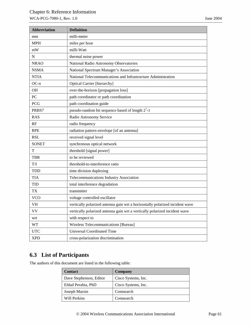
Chapter 6: Reference Information WCA-PCG-7080-1, Rev. 1.0 June 2004
© 2004 Wireless Communications Association International Page 61
Abbreviation Definition
mm milli-meter
MPH miles per hour
mW milli-Watt
N thermal noise power
NRAO National Radio Astronomy Observatories
NSMA National Spectrum Manager’s Association
NTIA National Telecommunications and Infrastructure Administration
OC-n Optical Carrier [hierarchy]
OH over-the-horizon [propagation loss]
PC path coordinator or path coordination
PCG path coordination guide
PRBS7 pseudo-random bit sequence based of length 27-1
RAS Radio Astronomy Service
RF radio frequency
RPE radiation pattern envelope [of an antenna]
RSL received signal level
SONET synchronous optical network
T threshold [signal power]
TBR to be reviewed
T/I threshold-to-interference ratio
TDD time division duplexing
TIA Telecommunications Industry Association
TID total interference degradation
TX transmitter
VCO voltage controlled oscillator
VH vertically polarized antenna gain wrt a horizontally polarized incident wave
VV vertically polarized antenna gain wrt a vertically polarized incident wave
wrt with respect to
WT Wireless Telecommunications [Bureau]
UTC Universal Coordinated Time
XPD cross-polarization discrimination
6.3 List of Participants The authors of this document are listed in the following table:
Contact Company
Dave Stephenson, Editor Cisco Systems, Inc.
Eldad Perahia, PhD Cisco Systems, Inc.
Joseph Marzin Comsearch
Will Perkins Comsearch

Chapter 6: Reference Information WCA-PCG-7080-1, Rev. 1.0 June 2004
© 2004 Wireless Communications Association International Page 62
Contact Company
John Lovberg, PhD LOEA Communications, Inc.
Thomas Rosa Terabeam Corporation
Thomas Wiltsey Terabeam Corporation
The following individual participated as an observer in the workshops employed to develop this document:
Contact Company
Mike Doolan National Telecommunications and Infrastructure Administration (NTIA)
6.4 List of WCA >60GHz Committee Voting Members The following individuals voted to approve this document at the June 21, 2004 meeting of the Over 60GHz Committee:
Contact Company
Doug Lockie Gigabeam Corporation (WCA 60+GHz Committee co-chair)
Randy Sifers Kelley Drye (Gigabeam Legal Counsel)
Ralph Booker Andrew Corporation
Gregg Levin Bridgewave Corporation
Moti Bordeley Ceragon Corporation
Hilik Shivek Ceragon Corporation
Joe Marzin Comsearch
Will Perkins Comsearch
Alex Kanarekin ElvaLink LLC
Don Brown International Wireless Packaging Consortium (IWPC)
Jay Lawrence LOEA Corporation
Mike Sharp Nokia
Randy Jenkins Stratex Networks
Robert Primosch Wilkinson Barker (WCA Legal Counsel)

Appendix A : Recommended Installation Practice WCA-PCG-7080-1, Rev. 1.0 June 2004
© 2004 Wireless Communications Association International Page 63
Appendix A: Recommended Installation Practice The following recommendations are provided to reduce the likelihood of inadvertent disruption of existing radio links during both the pre-installation planning and terminal installation phases. If temporary interruption of existing links is unavoidable, then permission to interrupt should be granted by the existing link owners prior to the disruption. This recommendation is crucial if the newly deployed link is involved in a bucking scenario (its transmitter is co-channel with a nearby incumbent receiver). All reasonable effort should be performed to minimize the down-time of the existing link.
(1) Pre-Installation Planning: Prior to installation, it is recommended that installers perform an onsite inspection and complete the following planning tasks before installing any terminals:
1. Select appropriate locations for all equipment considering path coordination with existing links.
2. Identify a suitable mounting structure (e.g. pole, wall, etc.) for the terminal.
3. Prepare a drawing detailing the location of all equipment, including the terminal, mounting structure, and all cable routing.
4. Develop a detailed cable routing and installation plan, including lengths and types of cables (copper and fiber).
5. Verify that network system equipment provided by others will be available at the specified locations during installation to minimize the number of potential disruptions to other links by work site personnel.
6. Paths must be unobstructed line-of-sight at all times (For example, roof-mounted terminals should be mounted high enough to allow for normal roof maintenance; allowance should be made for seasonal vegetation, growth of trees, power lines, snow buildup on the terminal or on any structures beneath the path, etc.).
(2) Installation (Initial Alignment): To minimize potential interference to existing links, each terminal should be mounted at the correct location as specified during path coordination (e.g., using instruments such as tape measures, GPS locators or transits) and “coarse” aligned without power applied using a spotting scope or camera boresighted to the antenna, or some other suitable means.
1. As a practical matter, a detachable, p.c.-compatible, digital video camera7 boresighted to the antenna, is an excellent alignment tool offering the following benefits:
• Quick, high resolution viewing of the LOS path on a lap-top computer
• Minimal recurring cost for each terminal
• Safe for installation personnel
• Better than ±1.5 degrees initial boresight accuracy8 easily achieved before powering-up the terminal
7 Industrial grade, high resolution, digital video cameras are available from several manufacturers, including Sony, Hitachi, Panasonic, and Basler; these cameras feature direct viewing on a personal computer via. an IEEE-1394 connection. As of the date of this document, cost for monochrome models is about $2,700. 8 Based on a mechanical tolerances study, assuming the antenna main beam has zero squint error from its mounting datum.

Appendix A : Recommended Installation Practice WCA-PCG-7080-1, Rev. 1.0 June 2004
© 2004 Wireless Communications Association International Page 64
2. If the area below the installation does not have restricted access, precautions must be taken to prevent hazards to people or property below, from accidentally falling objects (e.g. terminals, tools, etc.): use of safety “deadlines” (chains or lanyards) securely fastened to the terminal, other equipment, and tools, and a suitable structural support, is recommended.
(3) Installation (Final Alignment): To minimize potential interference to existing links during the final alignment procedure (when the terminal’s transmitter is radiating), the mount should have mechanical stops to limit boresight adjustment to the maximum necessary (typically ±1.5 degrees: refer to “Initial Alignment” above).
Figure A-1: Example of a detachable digital video camera, boresighted to the antenna used for initial alignment

Appendix B : Method for Measuring the C/I Required for Digital Receivers WCA-PCG-7080-1, Rev. 1.0 June 2004
© 2004 Wireless Communications Association International Page 65
Appendix B: Method for Measuring the C/I Required for Digital Receivers
A representative laboratory test setup for the receiver static threshold measurement is shown in Figure C-1 below. The mean output power of the modulated transmitter is first measured with a calibrated power detector. Peak power is assured to be 3 dB above mean power by virtue of a balanced modulation pattern. The transmitter is then coupled to the mated receiver, through a calibrated variable attenuator connected to the waveguide RF ports of each unit. Attenuation is increased until the receiver’s measured bit-error rate (BER) reaches 10-6. The product of the transmitter output power and the attenuation gives the receiver’s static threshold.
For instance, consider a transmitter with a measured average output power of 20 mW (+13 dBm) connected to a receiver under test as shown in Figure B-1. The calibrated attenuator is tuned to simulate path loss, and the measured BER reaches 1.0×10⁻⁶ at an attenuation of 67 dB. Then the measured static threshold is reported as +13 dBm – 67 dB = -54 dBm. For best precision, the measurement is repeated with a large calibrated fixed attenuator in front of the variable attenuator, dropping the variable attenuator nearer to the lower end of its range where it is most precise.
Figure B-1: Laboratory setup for measurement of receiver static threshold
The measurement of threshold-to-interference ratio T/I involves the injection of an interference signal into the setup shown in Figure B-1. This is accomplished using a calibrated coupler and noise generator as shown in Figure B-2. The attenuator is backed off by 1.0 dB from its value at static threshold (for higher precision, fixed attenuators have been substituted to provide the bulk of the required attenuation, such that the variable attenuator reads near the low end of its range at static threshold).
Transmitter Receiver
Cal Att

Appendix B : Method for Measuring the C/I Required for Digital Receivers WCA-PCG-7080-1, Rev. 1.0 June 2004
© 2004 Wireless Communications Association International Page 66
Figure B-2: Laboratory setup for measurement of receiver threshold-to-interference ratio
For instance, in the example given above the variable attenuator is reduced to provide a total path attenuation of -66 dB, raising the received power to -53 dBm, and the measured BER moves down to 6.5×10⁻⁸. Noise is then injected at the coupler to bring the bit-error rate back up to 10-6, and the noise level producing this BER is reported as the threshold interference level. It is further recommended that three types of interfering sources be considered and reported for purposes of interference coordination:
Broadband Noise A broadband noise source, band-limited at the receiver bandwidth and swept in frequency, is constructed using an amplified and filtered Johnson noise source. For instance, assuming a 2 GHz receiver bandwidth, an amplifier at 4-6 GHz might is terminated at its input to generate a thermal noise output. This output is mixed with a swept VCO at 77-80 GHz. At the VCO frequency of 77 GHz, the lower noise sideband at 71-73 GHz minimally overlaps a receiver centered at 73.5 GHz. When the VCO frequency is raised to 78.5 GHz, the overlap is at maximum, and at 80 GHz, it is again minimal. At the same VCO frequencies of 77, 78.5, and 80 GHz, the upper sideband minimally, maximally, and again minimally overlaps an 83.5 GHz transceiver. For each value of frequency within the entire 71-76 GHz or 81-86 GHz band (in 100-MHz increments), the coupled noise power is increased by way of a second variable attenuator until the bit error rate reaches 10-6, and the power level of the injected noise (through the attenuator and coupler) is reported. The result, in this example, is a spectral plot of T/I over 50 frequency points encompassing each receiver band.
CW Interferer A swept frequency generator provides the requisite signal for the narrowband interference measurement. Here again the source is swept across the receiver’s sensitive bandwidth and is adjusted in power until the receiver bit-error rate reaches 10-6. This power level is recorded for each value of the frequency in 100-MHz increments. The result is a spectral plot of T/I over 50 points across the receiver band. A typical T/I curve that might be reported for narrowband interference to a specific receiver, taken across the entire 71-76 GHz band, is shown in Figure B-3 below. In this example the receiver shows its highest sensitivity to tones near 73 GHz (presumably the desired carrier frequency), with strong sensitivity over about 2 GHz of bandwidth (presumably the spectral width of the desired data signal).
Transmitter Receiver
Cal Att
Noise Source
Cal Att
Att
-20 dB Coupler

Appendix B : Method for Measuring the C/I Required for Digital Receivers WCA-PCG-7080-1, Rev. 1.0 June 2004
© 2004 Wireless Communications Association International Page 67
T/I Curve for Narrowband Noise, Radio Model 123-456
- 4 0
- 3 0
- 2 0
- 10
0
10
2 0
3 0
4 0
7 1 7 2 7 3 7 4 7 5 7 6
Ce nt e r ba nd Fr e que nc y of In t e r f e r i ng S i gna l ( GHz )
Figure B-3: Example threshold-to-interference ratio curve for a receiver subjected to a narrowband interferer
Like-Signal Interferer A transmitter of the same type as that in the link under test is used to provide a third interference waveform. The interfering transmitter is modulated with a second bit generator, or, alternatively, with the same generator used for the link under test, after delaying the randomly modulated signal sufficiently to produce an uncorrelated data stream. The interference power level is adjusted by way of the variable attenuator until the bit error rate reaches 10-6, and the injected power level (through the variable attenuator and coupler) is reported as a scalar value.
For instance, following the example from the threshold measurement discussion above, adding coupled noise from a like transmitter modulated with a pseudo-random digital test signal, the BER reaches 1.0×10⁻⁶ when the interfering signal reaches –81dBm. This level is 27 dB below the reported static threshold level of -54 dBm, so the threshold-to-interference ratio T/I is reported as -54 dBm – (-81) dBm = 27 dB.
In the case where a specific receiver has the capability to be tuned to two or more frequency channels within either the 71-76 or 81-86 GHz band, it is recommended that equipment manufacturers repeat this measurement to report adjacent channel interference as well as co-channel interference.

Appendix B : Method for Measuring the C/I Required for Digital Receivers WCA-PCG-7080-1, Rev. 1.0 June 2004
© 2004 Wireless Communications Association International Page 68
This page intentionally left blank.

Appendix C : Method for Measuring the C/I Required for an Analog Receiver WCA-PCG-7080-1, Rev. 1.0 June 2004
© 2004 Wireless Communications Association International Page 69
Appendix C: Method for Measuring the C/I Required for an Analog Receiver
This appendix will be completed in a subsequent version of the document. Until this appendix is written, path coordination activities may not provide the same level of interference protection and certainty as for digital systems.

Appendix C : Method for Measuring the C/I Required for an Analog Receiver WCA-PCG-7080-1, Rev. 1.0 June 2004
© 2004 Wireless Communications Association International Page 70
This page intentionally left blank.
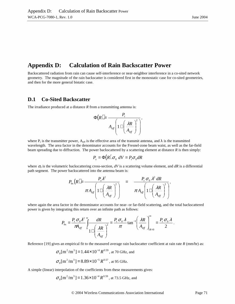
Appendix D: Calculation of Rain Backscatter Power WCA-PCG-7080-1, Rev. 1.0 June 2004
© 2004 Wireless Communications Association International Page 71
Appendix D: Calculation of Rain Backscatter Power Backscattered radiation from rain can cause self-interference or near-neighbor interference in a co-sited network geometry. The magnitude of the rain backscatter is considered first in the monostatic case for co-sited geometries, and then for the more general bistatic case.
D.1 Co-Sited Backscatter The irradiance produced at a distance R from a transmitting antenna is:
( )
+
=Φ2
1eff
eff
t
A
RA
PR
λ,
where Pt is the transmitter power, Aeff is the effective area of the transmit antenna, and λ is the transmitted wavelength. The area factor in the denominator accounts for the Fresnel-zone beam waist, as well as the far-field beam spreading due to diffraction. The power backscattered by a scattering element at distance R is then simply:
( ) dRPdVRP ts 00 σσ =Φ=
where σ0 is the volumetric backscattering cross-section, dV is a scattering volume element, and dR is a differential path segment. The power backscattered into the antenna beam is:
( )
+
=
+
=2
20
2
2
11eff
eff
t
effeff
sbs
A
RA
dRP
A
RA
PRP
λπ
λσ
λπ
λ,
where again the area factor in the denominator accounts for near- or far-field scattering, and the total backscattered power is given by integrating this return over an infinite path as follows:
2tan
1
0
0
10
02
20 λσλ
πλσ
λπλσ t
Reff
t
eff
eff
tbs
P
A
RP
A
R
dR
A
PP =
=
+
=∞
=
−∞
∫ .
Reference [19] gives an empirical fit to the measured average rain backscatter coefficient at rain rate R (mm/hr) as:
59.04320 1044.1]/mm[ R−×=σ , at 70 GHz, and
57.05320 1089.8]/mm[ R−×=σ , at 95 GHz.
A simple (linear) interpolation of the coefficients from these measurements gives:
59.04320 1036.1]/mm[ R−×=σ , at 73.5 GHz, and

Appendix D: Calculation of Rain Backscatter Power WCA-PCG-7080-1, Rev. 1.0 June 2004
© 2004 Wireless Communications Association International Page 72
58.04320 1014.1]/mm[ R−×=σ , at 83.5 GHz.
The corresponding backscatter ratios are thus:
59.071077.2 RP
P
t
bs −×= , at 73.5 GHz, and
58.071005.2 RP
P
t
bs −×= , at 83.5 GHz.
These results are plotted in Figure D-1. The simple mathematical treatment given above neglects the effect of beam attenuation by absorption and secondary forward scattering; however, beam attenuation due to water can be significant at rain rates above 10 mm/hr and must be considered in calculating total backscatter return. Since half of the return is due to near-field scatter, and the near field boundary for a 2-ft dish antenna is near 50m, an estimate of this effect is given by considering the attenuation of the propagating beam over that distance. At a rain rate of 100 mm/hr, beam attenuation over 50m is approximately 1.5 dB. The near-field scatter, which itself accounts for half of the total return power, is reduced by somewhat less than 1.5 dB, since the average two-way propagation distance of the scattered radiation represented by the near-field term is 50m. The far-field return is reduced by a factor greater than 1.5 dB because of the longer propagation paths it represents; the net effect is about a 1.5 dB overall reduction in the total return power. Taking this effect into account, the backscatter return flattens out slightly for higher rain rates as shown in Figure D-1.
Rain Backscatter
-75.00
-70.00
-65.00
-60.00
-55.00
-50.00
0.1 1 10 100 1000
Rain Rate (mm/hr)
Bac
ksca
tter
Po
wer
Rat
io (
dB
)
Backscatter Ratio (73.5 GHz)
Backscatter Ratio (83.5 GHz)
w/ attenuation (73.5 GHz, 2 ft. dish)
w/ attenuation (83.5 GHz, 2 ft. dish)
Figure D-1: Rain backscatter power relative to transmitted power
A transceiver may require up to 115 dB of transmit/receive isolation; much more isolation than rain backscatter will allow. Automatic Transmitter Power Control is irrelevant in this situation since transmitters will tend to operate at maximum power during strong rain events. Cross-polarizing the receive channel relative to the transmitter in principle provides additional isolation (rain induced depolarization is negligible for the short reflection paths making up most of the backscatter contribution), but still does not allow for clustering transceiver nodes on a rooftop. Dual-band frequency-division duplexing can eliminate this self-interference problem for a single transceiver; co-sited

Appendix D: Calculation of Rain Backscatter Power WCA-PCG-7080-1, Rev. 1.0 June 2004
© 2004 Wireless Communications Association International Page 73
backscatter interference can likewise be eliminated by using harmonized FDD via a coordinated band plan.
D.2 Near-Sited Rain Scattering The near-sited, or bistatic, rain-scattered interference geometry is shown in Figure D-2.
Figure D-2: Rain-scattered bistatic interference geometry
For an antenna separation distance d and victim and interfering antenna pointing angles θv and θi respectively (angles pointing inward are both taken positive by definition), the distance between each antenna and the scattering volume, in terms of the antenna separation and pointing angles, is:
( ) ( ).sin
cos and ,
sin
cos
iv
vi
iv
iv
dR
dR
θθθ
θθθ
+=
+=
The irradiance produced by the interferer at the location of the scattering volume is:
( ) ,
1
2
,,
+
=Φ
ieff
iieff
ti
A
RA
PR
λ
where Pt is the interfering transmitter power, Aeff,i is the effective area of the interfering transmitter’s antenna, and λ is the transmitted wavelength. The area factor in the denominator accounts for the Fresnel zone beam waist as well as the far-field beam spread due to diffraction. The power reflected by the scattering element in the direction of the victim is then simply:
( ) ( ) ,dVRP viis θθσ +Φ=
where σ(θ) is the angular-dependent scattering cross-section and dV is a scattering volume element.
The scattered power received by the victim antenna is likewise:
S
Rv
V
Ri
I d
θθθθi θθθθv
H
dV
Scattering volume
dRv
Victim beam cross-section

Appendix D: Calculation of Rain Backscatter Power WCA-PCG-7080-1, Rev. 1.0 June 2004
© 2004 Wireless Communications Association International Page 74
( ) ,
1
2
,,
2
+
=
veff
vveff
svv
A
RA
PRP
λπ
λ
where again the area factor in the denominator accounts for near- or far-field scattering.
Using the approximations that: 1) the irradiance produced by the interferer at smaller volume elements within a cross-sectional slice of the scattering volume (as shown in Figure D-2) is constant, and 2) variations in θv within the scattering volume are negligible, the scattered power integral becomes one-dimensional. The first approximation is less valid in the near field but adequate for estimating interference in all practical scenarios of interest to within 1 dB.
The second approximation is typically quite good. Noting also that Ri = Rv*cos(θv)/cos(θi), the power received by the victim antenna becomes:
( )∫
+
+=max,
min,
2
,
,
2
cos
cos1
v
v
R
R
iieff
vv
v
ieff
vitv
A
R
dR
A
PP
θθλπ
λθθσ
.)cos(
)cos(tan
)cos(
)cos(tan
)cos(
)cos()(
,
min_1
,
max_1
−
+= −−
i
v
ieff
v
i
v
ieff
v
v
iivt
A
R
A
RP
θθλ
θθλ
θθ
πλθθσ
The bounds on the integral are given in terms of the interfering dish diameter Di by:
.
2sin
2cos and ,
2sin
2cos
max,min,
−+
−
=
++
+
=
ivi
ii
v
ivi
ii
v
D
DdR
D
DdR
λθθ
λθ
λθθ
λθ
For far-field distances where the arctangent arguments are greater or equal to 1, the equation reduces to the well known form:
( ) ( )( ) .
11
cos
cos
2
11
cos
cos
max,min,2
2
2
2
max,min,2
2,
−
+=
−+=
vvv
ivitt
vvv
iieffvitv RR
GP
RR
APP
θθ
πθθσλ
θθ
πθθσ
Using the empirical cross-sections as before:
σ0[m2/m3] = 1.36 × 10⁻⁴ R0.59, at 73.5 GHz, and
σ0[m2/m3] = 1.14 × 10⁻⁴ R0.58, at 83.5 GHz,
an example calculation is given below, for a victim antenna pointing angle of 0°, an interfering antenna gain of 50 dB, a transmit frequency of 83.5 GHz, and a rain rate of 42 mm/hr (σ0 = 0.001 m2/m3):

Appendix D: Calculation of Rain Backscatter Power WCA-PCG-7080-1, Rev. 1.0 June 2004
© 2004 Wireless Communications Association International Page 75
Figure D-3: Rain backscatter for bistatic case as a function of separation distance and pointing angle
For this calculation, the scattering cross-section is assumed constant with angle; this should be true for angles of a few tens of degrees, but may be overly conservative at larger angles.
In the typical case, where the closest interaction distance of the interfering and victim beam centerlines is greater than zero (imperfect overlap), a multiplicative factor 0 ≤ γ ≤1 must be included to account for radiation suppression from the interfering and victim antenna pattern envelopes at the point of closest approach. An accommodation must also be added to the scattered power calculation to account for signal power attenuation in rain; i.e. secondary scattering events. In heavy rain the depth of the effective scattering volume can be determined not only by the geometrical factors but by the signal attenuation as well. In the example shown above, the 80 dB isolation predicted between two dishes separated by 100m and 10° is insufficient by itself (by 36 dB) to clear a worst-case interfering transmitter with +35 dBm transmit power and receiver with an interference threshold at -81 dBm. However, at 42 mm/hr, signal attenuation due to rain is 16 dB/km, and the scattering volume is about 560m away, so the two-way path signal attenuation is 18 dB. Another 18 dB of isolation is required, which may be realized if elevation differences between beams limit the overlap, and thus the interfering power level in the peak scattering volume. A difference of only 1.2° in elevation will add 22 dB or more of isolation in this case (following recommended FCC radiation pattern envelope restrictions). If scattered radiation cannot be cleared by these means, beam cross-polarization or a harmonized frequency plan may be required.
)(dBP
P
t
v
θi (degrees)
R = 42 mm/hr G = 50 dBi No rain attenuation σ(θ) = σ(0)
d =100 m
d =200 m
d =400 m