path following for a car-like mobile robot based on fuzzy-logic

International Master’s Thesis

Path Following for a Car-like Mobile Robot based onFuzzy-logic

Wenjie LinTechnology

Studies from the Department of Technology at Örebro University 0örebro 2012

Path Following for a Car-like Mobile Robot based onFuzzy-logic

Studies from the Department of Technologyat Örebro University 0

Wenjie Lin

Path Following for a Car-like MobileRobot based on Fuzzy-logic

© Wenjie Lin, 2012

Title: Path Following for a Car-like Mobile Robot based on Fuzzy-logic

ISSN 1650-8580

Abstract

The aim of this Master’s thesis is to investigate a path following approach forcar-like robots using fuzzy logic. The approach takes into account the vehiclenon-holonomic constraints. The thesis covers also the generation of a continu-ous path given a set of waypoints. The continuous path is modeled using uni-form cubic splines. The method is evaluated using a simulated robot running inthe 2D simulator Stage, part of the Player robot middleware.

i

Acknowledgements

I am sincerely thankful to my supervisor Abdelbaki Bouguerra for his helpfulguidance during this work, I would also thank Amy Loutfi and Jonas Ullbergfor their enthusiastic help.

iii

Contents

1 Introduction 11.1 Aim of the thesis . . . . . . . . . . . . . . . . . . . . . . . . . . 11.2 Motivation . . . . . . . . . . . . . . . . . . . . . . . . . . . . . 11.3 Work description . . . . . . . . . . . . . . . . . . . . . . . . . . 2

1.3.1 Research objectives . . . . . . . . . . . . . . . . . . . . . 21.3.2 Limitations . . . . . . . . . . . . . . . . . . . . . . . . . 21.3.3 Development work . . . . . . . . . . . . . . . . . . . . . 3

1.4 Organization . . . . . . . . . . . . . . . . . . . . . . . . . . . . 3

2 Background and Related work 52.1 Car-like vehicles . . . . . . . . . . . . . . . . . . . . . . . . . . . 52.2 Path generation and modeling . . . . . . . . . . . . . . . . . . . 62.3 Path following . . . . . . . . . . . . . . . . . . . . . . . . . . . 7

2.3.1 Traditional control . . . . . . . . . . . . . . . . . . . . . 82.3.2 Neural prediction controllers . . . . . . . . . . . . . . . 82.3.3 Reinforcement Learning . . . . . . . . . . . . . . . . . . 92.3.4 Hybrid methods . . . . . . . . . . . . . . . . . . . . . . 102.3.5 Fuzzy controllers . . . . . . . . . . . . . . . . . . . . . . 10

3 Continuous path generation using B-splines 153.1 Description . . . . . . . . . . . . . . . . . . . . . . . . . . . . . 153.2 Path representation . . . . . . . . . . . . . . . . . . . . . . . . . 163.3 Spline modification . . . . . . . . . . . . . . . . . . . . . . . . . 173.4 Collision checking . . . . . . . . . . . . . . . . . . . . . . . . . 19

4 Path following using Fuzzy logic 214.1 Knowledge base of fuzzy controller . . . . . . . . . . . . . . . . 21

4.1.1 Fuzzification . . . . . . . . . . . . . . . . . . . . . . . . 224.1.2 Rule inference . . . . . . . . . . . . . . . . . . . . . . . . 224.1.3 Defuzzification . . . . . . . . . . . . . . . . . . . . . . . 23

4.2 Design of the fuzzy controller . . . . . . . . . . . . . . . . . . . 23

v

vi CONTENTS

4.2.1 Position error control . . . . . . . . . . . . . . . . . . . . 244.2.2 Orientation error control . . . . . . . . . . . . . . . . . . 284.2.3 The structure of the fuzzy controller . . . . . . . . . . . 28

5 Experiments and evaluation 315.1 Implementation . . . . . . . . . . . . . . . . . . . . . . . . . . . 315.2 Newton-Rhapson method . . . . . . . . . . . . . . . . . . . . . 345.3 Position errors and orientation errors analyze . . . . . . . . . . 36

6 Conclusions 416.1 Summary . . . . . . . . . . . . . . . . . . . . . . . . . . . . . . 416.2 Further work . . . . . . . . . . . . . . . . . . . . . . . . . . . . 41

References 43

Chapter 1Introduction

1.1 Aim of the thesis

This thesis is the result of a master’s degree project done at AASS Learning Sys-tem lab. The aim of the current work is to develop control strategies to followpaths by car-like robots. The results of this work can, therefore, be implementedon vehicles destined to operate safely in dynamic environments.

1.2 Motivation

Car-like Mobile Robots have been widely researched with the goal to use themin application areas such as industry, military, mining, planet exploration, etc[2]. Such robot systems are considered as vehicles whose kinematic models ap-proximate the mobility of a car. Path following is one of the essential motiontasks for robots where a robot tries to reach and follow a geometric path (repre-sented as a set of oriented waypoints from a given initial configuration) withouthuman intervention. The position and orientation of robot’s main body and theangle of the steering wheels form the configuration of the robot. To achieve thistask in the classical approach, stationary obstacles and configuration of mobilerobot are presented in a two-dimensional map, the waypoints are generated bya planner that has to take into account the geometrical structure and kinemat-ics of the robot. The generated path contains waypoints with feasible curvaturethat avoid collision with obstacles. Modifying the path in advance is effectivefor robot system since it is much easier for the robots to achieve the motionautonomy in a priori known and well-modified environment, robots can movewithout receiving extra visual or range information. Besides, generating smoothpaths can avoid non-smooth motions that may lead to slipping of the wheelsand reduce the robot’s dead-reckoning ability. After obtaining the smooth path,the controller guides the vehicle to follow this path as closely as possible at exe-cution time. The motivation for using a fuzzy controller to follow the path is itsability to handle complex systems in a manner inspired from human expertise.

1

2 CHAPTER 1. INTRODUCTION

1.3 Work description

Car-like robots have kinematics constraints, specifically, they can not drive side-ways or rotate in place. They may need to perform many manoeuvres to reachthe target position. For example, they may need to stop and move backwardsin order to take a sharp turn. Such constraints that limit the possible direc-tions of motion at a point but can be “undone” by local maneuvering is callednonholonomic constraints [23]. "Since nonholonomic control systems are non-linear systems in essence, linear control strategies can’t be used directly to solvesuch kind of problems" [25].

1.3.1 Research objectives

This thesis is intended to do some introductory research in the area of path fol-lowing by mobile vehicles. The chief goal is developing a softerware controllerto achieve smooth and collision-free path following.

The input of the system is a set of waypoints and a group of polygonalobstacles. The waypoints are determined by both position and orientation. Toachieve our goal, we should first generate a continuous path to connect all thegiven waypoints. Because car-like robots have steering constraints, the curva-ture of the generated path should be easy to modify. Cubic B-splines are adaptedin this work, since the curvature can simply be obtained by a function that op-erates on the derivatives of the curve. Besides, cubic B-splines allow sectionaladjustments by moving some of their control points.

To achieve path following, the thesis presents a fuzzy controller that is testedin a 2D multiple-robot simulator. Even if the working environment is well-known, sensor signal is uncertain and imprecise, the robot itself, is a systemwhose kinematics and dynamics are complex and non-linear, hence it is hardto find an adaptive control system which is accurate and complete. Intelligentcontrol theory [31] has been φ: the wheel steering angle.introduced to solvecomplex nonlinear behavior problems. Fuzzy controller, whose main compo-nent is a set of fuzzy rules encoding the reactive behaviors of the vehicle, isbased on typical intelligent control. It is the control mechanism that straight-forwardly handles the problems of behavior arbitration and command fusion.This permits an easy and incremental construction of the fuzzy rule base andalso to develop and test the basic behaviors separately.

1.3.2 Limitations

Although the principle tasks were implemented and the expected goal has beenachieved, still some issues are ignored and many capabilities can be improvedin future work.

Firstly, only stationary obstacles were considered. In this project, the work-ing environment is assumed to be static. That is, the obstacles are stationary

1.4. ORGANIZATION 3

and neither added nor removed at execution time. Moving objects(obstacles)are not considered in this work. Thus the continuous path generation is lim-ited to simple environments. Therefore, there’s lack of capabilities for handlingemergency cases.

Secondly, only path-forward motion was considered. In the developed behavior-based approach, the robot is assumed to follow the generated path by forwardmotion. i.e., the robot never moves backwards. Because the environment iscompletely known and stationary, only wheel turning e.g. right-low, right-high,left-low, left-high was used to tune the orientation and position errors. This ap-proach makes the robot reach the target as soon as possible. But only forwardand turning motions are not enough sometimes, as they can result in inefficien-cies and deadlock situations.

1.3.3 Development work

The implementation of the path following controller has been done in C++programming language. The controller was implemented as a Player driver [6].The testing and evaluation were carried using the 2D simulator Stage.

1.4 Organization

This thesis is organized as follows:

• Chapter 2 introduces background and related work. The chapter includesalso a summary of different robot controllers with an emphasis on fuzzylogic.

• Chapter 3 presents an approach of building uniform cubic B-splines pathsgiven for sets of oriented waypoints.

• Chapter 4 describes work to develop a fuzzy controller, several rules rep-resenting behaviors of an intelligent system have been established. Thefuzzy controller is implemented as a Player driver.

• Chapter 5 reports experiments for testing and evaluating the developedcontroller.

• Chapter 6 summarizes the work developed in this thesis. It also discussesthe obtained results and concludes with remarks regarding possible direc-tions for future work.

Chapter 2Background and Related work

This chapter gives some background of the material presented in this thesis.The first part describes the features and constraints of car-like robots that makethe path following more complex. The second part gives a summary overviewof the existing methods on generating the continuous path by a given set ofwaypoints. A particular way of path generation is based on cubic B-splines. Thespline function and modification will be explained in detail in the next chapter.The rest of chapter introduces the main types of existing controllers of pathfollowing category based on artificial intelligence; such as neural prediction,reinforcement learning and hybrid methods, the advantage of fuzzy controlleris emphasized and a brief introduction of fuzzy theory is given in the end of thischapter.

2.1 Car-like vehicles

A Car-like robot (see Figure 2.1) has similar locomotion structure to a car. Itis a mobile vehicle whose two front wheels can be steered in parallel and thetwo rear wheels are parallel and fixed. Car-like robots can’t drive sidewayssince they are not able to rotate in place. Car-like robots can be consideredas a three-dimensional system moving on the plane. Their motions are limitedby non-slipping and curvature constraints. The minimal length paths for suchrobots are composed by a finite sequence of arcs of circles and straight-linesegments. However, the curvatures of these two parts are discontinuous. If therobot wants to follow such a path, it has to stop at the points whose curvaturesare discontinuous to adjust its angular velocity and linear velocity. Therefore,the key problem of related research is how to generate a path that has continu-ous curvature. In the figure 2.1, x and y are the coordinates of robot’s positionin XY frame, θ is the vehicle’s orientation angle, φ is vehicle’s steering angle,R is the middle point of rear axle which represents the origin of the vehiclereference frame, l is the distance between wheel axles, v is the linear velocity ofpoint R. The motion is expressed as in Equation (2.1) [7].

5

6 CHAPTER 2. BACKGROUND AND RELATED WORK

q

x

y

f

X

Y

R

l

v

Figure 2.1: A Car-like robot. (For the robots we consider in this thesis, a givenposition and orientation is known as a 3-tuple configuration (x,y, θ).)

x = v cos θ

y = v sin θ

θ =v

ltanφ

(2.1)

2.2 Path generation and modeling

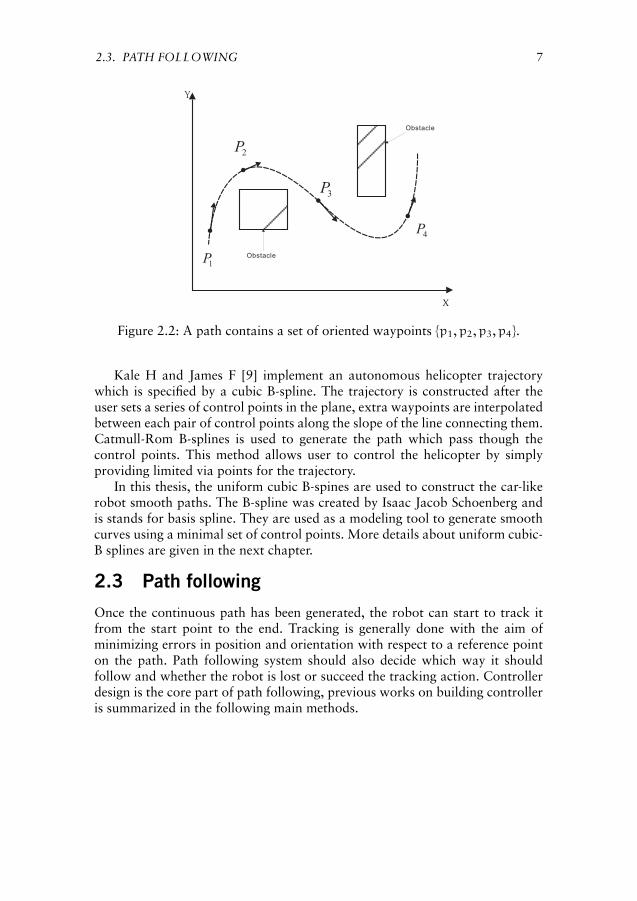
In this work, the input of the execution system is a set of discrete orientedwaypoints. As shown in Figure 2.2, the oriented waypoint set includes fourpoints, they are represented as {p1,p2,p3,p4}, each point is set into the mapwith both position coordinates and orientation that are represented by arrowline segments. A smooth path is a continuous curve that goes through eachwaypoint while avoiding collision with the obstacles in the meantime. To solvethe path-planning problem, many prior works use different splines to generatesmooth paths. John C and Gabriel E [3] have presented a method to generatean efficient and collision free path by bending and adjusting a B-spline. Jung-Hung H and Arkin R [11] realized a supervisory control by generating a Beziercurve on-line trajectory. Shin D and Singh S [20] using clothoidal curves tobuild a trajectory for robot vehicles. Wagner P and Kotzian J [24] discussedpath planning and tracking based on cubic hermite splines in real-time.

2.3. PATH FOLLOWING 7

1P

2P

3P

4P

x

Y

Obstacle

Obstacle

Figure 2.2: A path contains a set of oriented waypoints {p1,p2,p3,p4}.

Kale H and James F [9] implement an autonomous helicopter trajectorywhich is specified by a cubic B-spline. The trajectory is constructed after theuser sets a series of control points in the plane, extra waypoints are interpolatedbetween each pair of control points along the slope of the line connecting them.Catmull-Rom B-splines is used to generate the path which pass though thecontrol points. This method allows user to control the helicopter by simplyproviding limited via points for the trajectory.

In this thesis, the uniform cubic B-spines are used to construct the car-likerobot smooth paths. The B-spline was created by Isaac Jacob Schoenberg andis stands for basis spline. They are used as a modeling tool to generate smoothcurves using a minimal set of control points. More details about uniform cubic-B splines are given in the next chapter.

2.3 Path following

Once the continuous path has been generated, the robot can start to track itfrom the start point to the end. Tracking is generally done with the aim ofminimizing errors in position and orientation with respect to a reference pointon the path. Path following system should also decide which way it shouldfollow and whether the robot is lost or succeed the tracking action. Controllerdesign is the core part of path following, previous works on building controlleris summarized in the following main methods.


PID Mobile robot model

errorInput Output

+-

å å

Figure 2.3: The structure of PID controller [15].

2.3.1 Traditional control

Traditional control systems are based on the concept of feedback. Value innegative feedback is calculated by an “error” as the difference between a mea-sured process variable and a desired value. This kind of controller attempt tominimize the error by adjusting the process control inputs. A. De Luca andG. Oriolo described a very detailed way of using feedback control techniquesto achieve car-like robot motion tasks [14]. Most of the applications belongto the form of closed-loop control. One of the developed closed-loop controlis PID (Proportional-Integral-Differential) control. It requires three terms op-erating on the error signal to produce a control signal Figure 2.3. Since PIDcontroller is easy to model, and it is robust, some researchers use it to buildthe path-tracking controller. In Julio E and Ismael A’s work [15], a PID basedpath tracking controller is successfully implemented in a synchro-drive mobilerobot. But it is only adapted to a linear model with simple parameters. Anotherform of control is on-off control. System output is in the form of on or off withthe movement provider. Servomechanism type control is widely used in robotpath planning as well. Servomechanism is one kind of automatic device thatuse error-sensing negative feedback to control mechanical position, speed orother parameters [26]. For the position control, the inputs are compared withthe actual positions that measured by sorts of transducer at the outputs. Anydifference between the actual and desired value is amplified and converted toreduce the error and lead the system go to acceptable area.

2.3.2 Neural prediction controllers

Some prior works use a neural predictive controller for path tracking. The ideaof predictive controller is computing a future control action that is based onoutput values predicted by a model [18]. Neural networks are an attractiveway to model complex non-linear systems due to their inherent ability to ap-proximate arbitrary continuous function. Gu D and Hu H [8] presents a model-based predictive controller(MPC) based on multi-layer back-propagation neu-ral network. As shown in Figure 2.4, the two basic value sources for networktraining are the desired states with control vector and the measured states.The path generation module produces the desired states, which are representedby Z (k) = [z (x) , z (y) , z (θ)], where k is the sample time. The control vec-


Figure 2.4: The structure of back propagation network [8].

tor consist of two variables, the speed of robot v(k − 1) and the steer angleα(k − 1). Both control vector and measured states formed the inputs of back-propagation neural network. The measured states are represented by the cur-rent states of robots, which obtained from the position estimation module asX (k− 1) = [x (k− 1) ,y (k− 1) , θ (k− 1)]T . Then the network start the for-wards training though the hidden layer functions, yielding outputs are repre-sented as X (k) = [x (k) ,y (k) , θ (k)]

T . The errors E between Z(k) and X(k) areobtained and set as feedback signals, which are further decomposed into tan-gential and normal errors. If E is larger than a threshold, the back propagationhappens, the weight of each hidden layer will be modified, and the iterationwill continue until the errors are small and less than the given thresholds.

2.3.3 Reinforcement Learning

Some of the researchers use the reinforcement learning strategies to controlrobot behavior. Reinforcement learning (RL) is a supervised learning [22], whichfine-tune the behavior by rewards or punishments. There are three main groupsof methods of RL, they are dynamic programming (DP) methods, monte carlo(MC) methods and temporal difference (TD) methods. They are divided by twofactors, models of the environment and bootstrapping. In RL system, Boot-strapping is used to update the estimate of state values and action values basedon the estimate of later states. DP requires both bootstrapping and completemodel of the environment. MC and TD methods do not require the model ofenvironment, and TD methods need do bootstrap but MC methods do not. Itis hard to use DP methods based on models of well-known environments, sincethe environment of the robot is the real world and it might change often. Onthe other hand, TD methods learn faster than MC methods during exploring


because of TD bootstrap allowed estimate to update other estimate, that is,TD methods update value after each time step, rather than after each episode.TD methods can know whether an explored choice is good or bad immediatelyand update the policy at each time step, they do not need to wait until theend of the episode to decide the policy is better or worse than previous one.So many researchers choose TD method to training the robot. Q learning is apopular method of TD methods. Lavi M and Sara K use Q learning to realizethe path following of a koolio robot [30]. J.Baltes and Yuming manage to use acase-based function approximator to expand the RL to deal with path-trackingproblem with a car-like robot [1]. Each case is represented as a collection of thestate and the action. Some of the cases that similar to the inputs are found togenerate a nearest neighbor set. Q learning is adapted to choose the next stateand update the system inputs.

2.3.4 Hybrid methods

In some previous works, to achieve more complicated motions, more than onecontroller is used to cooperate with each other in order to achieve better results.Philippe G and Cyril N implement a hybrid controller that is made of escapelines controller and fuzzy one on Praxitele cars [5]. The escape lines controllerbuilt the free escape lines set and compare with the catch-up curve which isbuilt by the path planner, then chose the nearest free escape line as the follow-ing path and send it to fuzzy controller. The fuzzy controller follows this pathtaking into account obstacles detected by sensors. By this hybrid controller,the priori given path by a path planner is adapted to the real and dynamicenvironment. Matthias H and Oliver W present a hybrid feedback controllerthat integrate a local obstacle-avoidance controller and a global path replan-ning controller for a mobile robot [10]. This controller enables collision-freetracking for preplanned path in both indoor and outdoor environments.

2.3.5 Fuzzy controllers

Fuzzy methods became one of the most popular ways to design controllersfor nonlinear, time varying and uncertain system. Fuzzy logic controllers arecheaper to develop, they cover a wider range of operating conditions, and theyare easier to understand in natural language terms [17]. As early as 1965, Zadehof California University published a first paper about fuzzy logic. Later he an-alyzed his ideas in a 1973 paper, which introduced the concept of “linguisticvariables” [29]. In 1987, Japanese researcher Takeshi Yamakawa demonstratedfuzzy control method by an “inverted pendulum” experiment [27].

Since path-tracking problem for nonhonolomic robots involves both kine-matics and dynamics difficulties and the interaction between the vehicle and theterrain may be hard to model in general, many studies focus on adopting thefuzzy logic control method to solve the path-tracking problems. In most of the


approaches, both position controller and orientation controller are developedto achieve the desired state [16, 4].

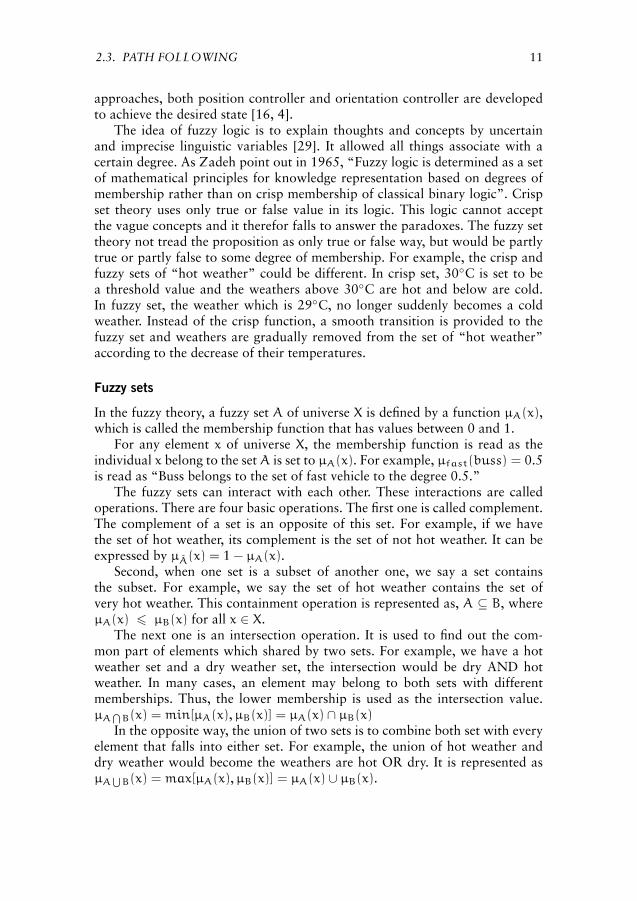
The idea of fuzzy logic is to explain thoughts and concepts by uncertainand imprecise linguistic variables [29]. It allowed all things associate with acertain degree. As Zadeh point out in 1965, “Fuzzy logic is determined as a setof mathematical principles for knowledge representation based on degrees ofmembership rather than on crisp membership of classical binary logic”. Crispset theory uses only true or false value in its logic. This logic cannot acceptthe vague concepts and it therefor falls to answer the paradoxes. The fuzzy settheory not tread the proposition as only true or false way, but would be partlytrue or partly false to some degree of membership. For example, the crisp andfuzzy sets of “hot weather” could be different. In crisp set, 30◦C is set to bea threshold value and the weathers above 30◦C are hot and below are cold.In fuzzy set, the weather which is 29◦C, no longer suddenly becomes a coldweather. Instead of the crisp function, a smooth transition is provided to thefuzzy set and weathers are gradually removed from the set of “hot weather”according to the decrease of their temperatures.

Fuzzy sets

In the fuzzy theory, a fuzzy set A of universe X is defined by a function µA(x),which is called the membership function that has values between 0 and 1.

For any element x of universe X, the membership function is read as theindividual x belong to the setA is set to µA(x). For example, µfast(buss) = 0.5is read as “Buss belongs to the set of fast vehicle to the degree 0.5.”

The fuzzy sets can interact with each other. These interactions are calledoperations. There are four basic operations. The first one is called complement.The complement of a set is an opposite of this set. For example, if we havethe set of hot weather, its complement is the set of not hot weather. It can beexpressed by µA(x) = 1 − µA(x).

Second, when one set is a subset of another one, we say a set containsthe subset. For example, we say the set of hot weather contains the set ofvery hot weather. This containment operation is represented as, A ⊆ B, whereµA(x) 6 µB(x) for all x ∈ X.

The next one is an intersection operation. It is used to find out the com-mon part of elements which shared by two sets. For example, we have a hotweather set and a dry weather set, the intersection would be dry AND hotweather. In many cases, an element may belong to both sets with differentmemberships. Thus, the lower membership is used as the intersection value.µA

⋂B(x) = min[µA(x),µB(x)] = µA(x) ∩ µB(x)

In the opposite way, the union of two sets is to combine both set with everyelement that falls into either set. For example, the union of hot weather anddry weather would become the weathers are hot OR dry. It is represented asµA

⋃B(x) = max[µA(x),µB(x)] = µA(x) ∪ µB(x).


T-norm T-conormMinimum/Maximum a∧ b a∨ b

Algebraic product/sum ab a+ b− ab

Algebraic product/sum 0 ∨ (a+ b− 1) 1 ∧ (a+ b)

Drastic product/sum

a if b = 1b if a = 10 a,b < 1

a if b = 0b if a = 01 a,b > 0

Table 2.1: T-norm and T-conorm operators.

In general, the intersection can be specified by T-norm (triangular norm)operators. A T-norm is a binary operator on [0, 1] which satisfying bound-ary, monotonicity ,commutativity and associativity. There is another class ofoperators, which refer to fuzzy union operation, called T-conorm. The justifi-cation of basic requirements for T-conorm is similar to that of the requirementsfor T-norm operators. Table 2.1shows the most frequently used T-norm and T-conorm operators. Assume that a and b are two membership functions between0 and 1 [12].

Fuzzy rules

Fuzzy rule-based system on fuzzy set theory is the most important tool to buildthe fuzzy controller. Fuzzy rule also known as fuzzy if-then rule, we can expressas the following form:

IF x is A THEN y is B.

where A and B are linguistic values defined by fuzzy sets on universes ofdiscourse X and Y. x and y are linguistic variables. This rule can be representedas A → B. For example, we can set the following rules to a fuzzy controller ofa robot:

IF road is smooth, THEN speed is fast.

IF road is rugged, THEN speed is slow.

Assume that a fuzzy if-then rule be defined as a binary fuzzy relation R onthe product space X. There are two ways to express the fuzzy rule A→ B. Oneof them is “A coupled with B” and the other one is “A entails B”.

If A → B is interpreted as A coupled with B, R = A → B = A × B =∫X×Y µA(x)⊗ µB(x)/(x,y), where ⊗ is a T-norm operator [12].

If A→ B is interpreted as A entails B, then it can be written as four differentformulas [12],


* Material implication: R = A→ B = ¬A ∪ B

* Propositional calculus: R = A→ B = ¬A ∪ (A ∩ B)

* Extended propositional calculus: R = A→ B = (¬A ∩ ¬B) ∪ B

* Generalization of modus ponens:µR(x,y) = sup{c|µA(x)⊗c 6 µB(x) 0 6c 6 1}

Fuzzy inference

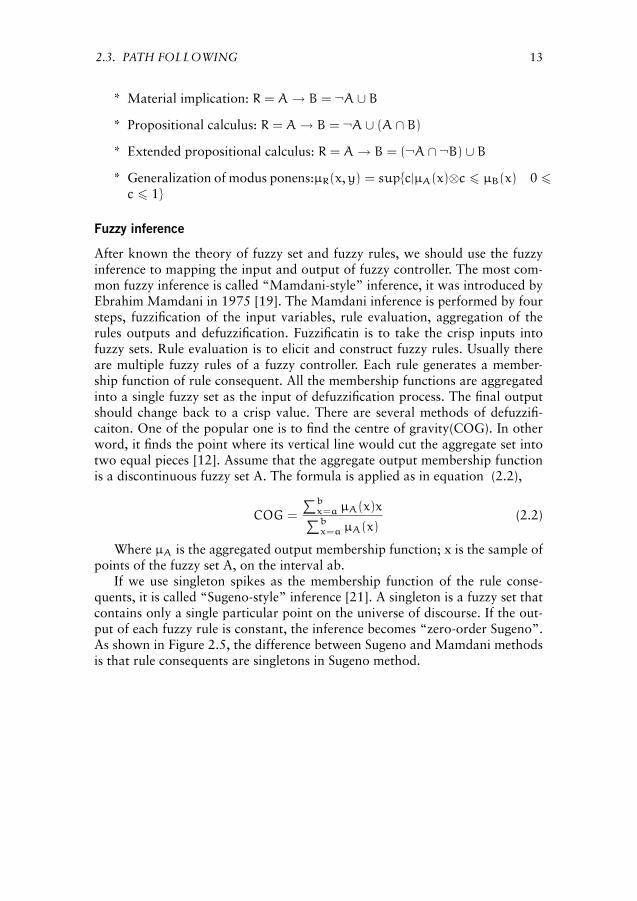
After known the theory of fuzzy set and fuzzy rules, we should use the fuzzyinference to mapping the input and output of fuzzy controller. The most com-mon fuzzy inference is called “Mamdani-style” inference, it was introduced byEbrahim Mamdani in 1975 [19]. The Mamdani inference is performed by foursteps, fuzzification of the input variables, rule evaluation, aggregation of therules outputs and defuzzification. Fuzzificatin is to take the crisp inputs intofuzzy sets. Rule evaluation is to elicit and construct fuzzy rules. Usually thereare multiple fuzzy rules of a fuzzy controller. Each rule generates a member-ship function of rule consequent. All the membership functions are aggregatedinto a single fuzzy set as the input of defuzzification process. The final outputshould change back to a crisp value. There are several methods of defuzzifi-caiton. One of the popular one is to find the centre of gravity(COG). In otherword, it finds the point where its vertical line would cut the aggregate set intotwo equal pieces [12]. Assume that the aggregate output membership functionis a discontinuous fuzzy set A. The formula is applied as in equation (2.2),

COG =

∑bx=a µA(x)x∑bx=a µA(x)

(2.2)

Where µA is the aggregated output membership function; x is the sample ofpoints of the fuzzy set A, on the interval ab.

If we use singleton spikes as the membership function of the rule conse-quents, it is called “Sugeno-style” inference [21]. A singleton is a fuzzy set thatcontains only a single particular point on the universe of discourse. If the out-put of each fuzzy rule is constant, the inference becomes “zero-order Sugeno”.As shown in Figure 2.5, the difference between Sugeno and Mamdani methodsis that rule consequents are singletons in Sugeno method.


1

AND(PROD)

0.20.4

0.08

1

AND(PROD)

0.20.4

0.08

Rule: If x is A1(0.2)And y is B1(0.4) Then z is C2(0.08)

Figure 2.5: The Mamdani rule evaluation(top) and The Sugeno rule evalua-tion(bottom).

Chapter 3Continuous path generationusing B-splines

A path generating method based on cubic B-splines is presented in this chapterto represent a path that connects all the waypoints that are given as the inputsof the control system. A stretch method is adapted to make the path avoidundesired and unnavigable situations, such as too large curvatures for robotsteering or too narrow space for robot passages though obstacles.

3.1 Description

As shown in Figure 3.1, the inputs of the path generator include a set of way-points and a group of obstacles. The waypoints have both position coordinates(x,y) and orientations. The obstacles are presented as a group of polygons on atwo-dimensional map. The output of path generator is represented as a feasiblepath that connects all the waypoints. The path satisfies both smoothness andcollision-free requirements.

1P

2P

3P

4P

1P

2P

3P

4P

Figure 3.1: The inputs and outputs of path generator. Left(input): Orientedwaypoints and obstacles; Right (Output):A continuous path passing throughthe given waypoints.

15

16 CHAPTER 3. CONTINUOUS PATH GENERATION USING B-SPLINES

In our work, we only consider the forward motion of car-like robots thatare not supposed to stop except at the final goal. Considering kinematics con-straints, there are two non-holonomic constraints, The robot can only movealong the main axle which is perpendicular to the rear wheels of robot, andthe front wheel’s steering angle is upper bounded. Therefore the required pathshould be smooth and its curvature should not be larger than the maximumone. On the other hand, collision-free paths are required, i.e., the robot has tofollow the path without colliding with obstacles.

3.2 Path representation

We choose uniform cubic B-splines as the path generating function which is atypical smooth function and its curvature is easy to obtain. A cubic B-splineformulation in t is written as:

St =

n−1∑i=0

PiNi,3(t) 0 6 t 6 1, n− 1 > 3 (3.1)

Where Pi are the control points and Ni,3 is normalized B-spline basis func-tion (blending function), t is a global parameter. n control points design n − 3segments and each segment is related to four control points [7],

The blending function of uniform cubic B-spline can easily be precalculatedand is equal for each segment in this case, it is given as in (3.2),

Si(t) =[t3 t2 t 1

] 16

−1 3 −3 1

3 −6 3 0

−3 0 3 0

1 4 1 0

Pi−1

Pi

Pi+1

Pi+2

(3.2)

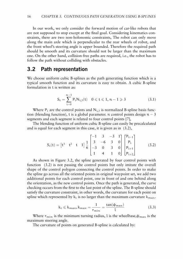
As shown in Figure 3.2, the spline generated by four control points withfunction (3.2) is not passing the control points but only imitate the overallshape of the control polygon connecting the control points. In order to makethe spline go across all the oriented points in original waypoint set, we add twoadditional points for each control point, one in front of and one behind alongthe orientation, as the new control points. Once the path is generated, the curvechecking occurs from the first to the last point of the spline. The B-spline shouldsatisfy the curvature constraint, in other words, the curvature for each point onspline which represented by ki is no larger than the maximum curvature kmax.

ki 6 kmax,kmax =1

rmin=

tan(φmax)

l(3.3)

Where rmin is the minimum turning radius, l is the wheelbase,φmax is themaximum steering angle.

The curvature of points on generated B-spline is calculated by:

3.3. SPLINE MODIFICATION 17

Figure 3.2: A uniform cubic B-spline specified by four control points{p0,p1,p2,p3}.

ki =|x ′y ′′ − y ′x ′′|

(x ′2 + y ′2)32

(3.4)

Where (x,y) is the coordinate of a point on the spline.

3.3 Spline modification

Curvature and collisions should be checked simultaneously. Once either thewrong curvature or obstacle collision is detected, the related segments should bemodified. As mentioned before, each segment is related to four control points,the control points are formed by the original inputs and the additional points.The curve can be modified by increasing or decreasing the stretch weight ofadditional points. When one additional control point changes, all the relatedsegments should be re-measured.

As shown in Figure 3.2, the control polygon is specified by the set of controlpoints.The curve tends to imitate the overall shape of the control polygon whileit passes none of the control points. After adding two extra points along theorientation of each control point, as shown in Figure 3.3, the path is availableto go across the original control points. The additional points is calculated byEquation (3.5),

18 CHAPTER 3. CONTINUOUS PATH GENERATION USING B-SPLINES

3 4 5 6 7 8 9 10 112.8

3

3.2

3.4

3.6

3.8

4

4.2

4.4

Wi=0.2

P3

P2P0

P1

Figure 3.3: A cubic B-spline specified by the original and the additional controlpoints. All points here were placed using wi = 0.2.

3 4 5 6 7 8 9 10 112.8

3

3.2

3.4

3.6

3.8

4

4.2

4.4

Wi=0.1

Wi=0.4

P1 P3

P0 P2

Figure 3.4: The shape of the curve changes by stretching the additional points,i.e.,by changing the values of the weights wi.

3.4. COLLISION CHECKING 19

0R

1R

2R

3R

0P

1P2

P

3P 4

P

O

Figure 3.5: Collision-free detecting of robot and obstacle.

a1 = pi +wiµ

a2 = pi −wiµ(3.5)

Where a1 and a2 are two additional points of pi , θ is the orientation ofpi. wi is the stretch weight and µ is a unit vector, such that µ = (cos θ, sin θ)T ,in Figure 3.3 wi is 0.2. As shown Figure 3.4, one of the curves is specified byadding two additional points for each control points by decrease wi to 0.1,while the other curve is obtained by increasing the wi to 0.4. It is obvious tosee that wi pulling the curve towards control points as it decreases or movingthe curve away as it increases.

In my work, the maximum steering angle is set to be pi/4, the maximumcurvature is calculated using equation (3.3). During the path modification, thepath turns smoother as long as the additional points move further from originalpoints. If the distance between the additional point and original point exceedthe maximum regulated distance we set, the modification process will end andindicate that there is no available path generated.

3.4 Collision checking

The continuous path, once generated, have to be checked for collision avoid-ance.

To detect whether a path is collision-free, we first load robot to current po-sition, as shown in Figure 3.5, the location of robot is represented by O whichis the middle of the robot’s rear axle. In two-dimensional map, we use a sim-ple math method to store the robot and the obstacle as two arrays of triangles{(R0R1R2), (R1R2R3)} and {(P0P1P2), (P1P2P3), (P3P4P1)}, here we use proximityquery package (PQP) to check whether pairs of triangles from different arraysare overlapping [13].

If a collision is detected, the segment of collision area would be selected andthe path modification starts with the related control points.

Chapter 4Path following using Fuzzylogic

In this chapter, we describe the fuzzy rule-based controller that was developed,as part of the work of this thesis, to control a mobile robot to follow a contin-uous path.

4.1 Knowledge base of fuzzy controller

In the fuzzy controller, each fuzzy variable is associated with a fuzzy set thatis characterized by its membership function. We use a piecewise function togenerate variety of membership functions. The function called “RampUp” isimplemented as,

RampUp(xl, xr, x) =

0 if x < xlx−xl

xr−xlif xl < x < xr

1 else(4.1)

Where xl is the left breakpoint and xr is the right breakpoint, then the Ramp-Down function is just reflection.

RampDown(xl, xr, x) =

1 if x < xlxr−xxr−xl

if xl < x < xr

0 else(4.2)

The Trapazoid function is implemented as a combination of the RampUpand RampDown function, “∩ ′′ operation is defined as minimum function whichbelong to T-norm operators.

Trapazoid(xcen, xd, xslope, x) = RampUp(xcen − xd − xsolpe, xcen − xd, x)∩RampDown(xcen + xd, xsolpe + xcen + xd, x)

(4.3)

21

22 CHAPTER 4. PATH FOLLOWING USING FUZZY LOGIC

0

1

Slow Medium Fast

Speed (m/s)

0.5

1

.

RampDown

Trapazoid RampUp

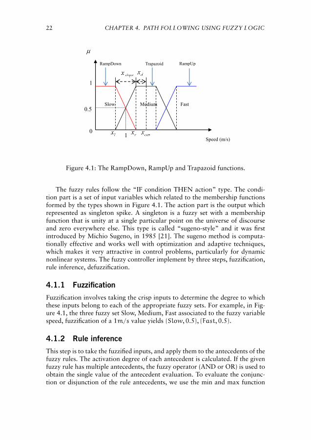
Figure 4.1: The RampDown, RampUp and Trapazoid functions.

The fuzzy rules follow the “IF condition THEN action” type. The condi-tion part is a set of input variables which related to the membership functionsformed by the types shown in Figure 4.1. The action part is the output whichrepresented as singleton spike. A singleton is a fuzzy set with a membershipfunction that is unity at a single particular point on the universe of discourseand zero everywhere else. This type is called “sugeno-style” and it was firstintroduced by Michio Sugeno, in 1985 [21]. The sugeno method is computa-tionally effective and works well with optimization and adaptive techniques,which makes it very attractive in control problems, particularly for dynamicnonlinear systems. The fuzzy controller implement by three steps, fuzzification,rule inference, defuzzification.

4.1.1 Fuzzification

Fuzzification involves taking the crisp inputs to determine the degree to whichthese inputs belong to each of the appropriate fuzzy sets. For example, in Fig-ure 4.1, the three fuzzy set Slow, Medium, Fast associated to the fuzzy variablespeed, fuzzification of a 1m/s value yields (Slow, 0.5), (Fast, 0.5).

4.1.2 Rule inference

This step is to take the fuzzified inputs, and apply them to the antecedents of thefuzzy rules. The activation degree of each antecedent is calculated. If the givenfuzzy rule has multiple antecedents, the fuzzy operator (AND or OR) is used toobtain the single value of the antecedent evaluation. To evaluate the conjunc-tion or disjunction of the rule antecedents, we use the min and max function

4.2. DESIGN OF THE FUZZY CONTROLLER 23

0.9

0

1

3m

Close

Distance

If And

Speed

Medium

5m/s

0.82

1Then

0.82

1

Braking-2m/s

Medium

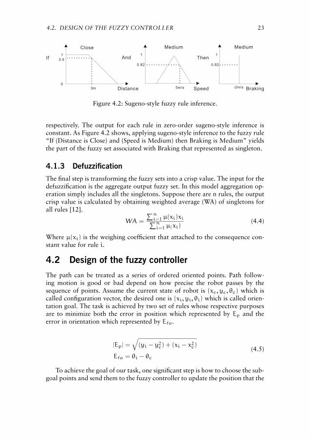
Figure 4.2: Sugeno-style fuzzy rule inference.

respectively. The output for each rule in zero-order sugeno-style inference isconstant. As Figure 4.2 shows, applying sugeno-style inference to the fuzzy rule“If (Distance is Close) and (Speed is Medium) then Braking is Medium” yieldsthe part of the fuzzy set associated with Braking that represented as singleton.

4.1.3 Defuzzification

The final step is transforming the fuzzy sets into a crisp value. The input for thedefuzzification is the aggregate output fuzzy set. In this model aggregation op-eration simply includes all the singletons. Suppose there are n rules, the outputcrisp value is calculated by obtaining weighted average (WA) of singletons forall rules [12].

WA =

∑ni=1 µ(xi)xi∑ni=1 µ(xi)

(4.4)

Where µ(xi) is the weighing coefficient that attached to the consequence con-stant value for rule i.

4.2 Design of the fuzzy controller

The path can be treated as a series of ordered oriented points. Path follow-ing motion is good or bad depend on how precise the robot passes by thesequence of points. Assume the current state of robot is (xc,yc, θc) which iscalled configuration vector, the desired one is (xi,yi, θi) which is called orien-tation goal. The task is achieved by two set of rules whose respective purposesare to minimize both the error in position which represented by Ep and theerror in orientation which represented by Efo.

|Ep| =

√(yi − y2

c) + (xi − x2c)

Efo = θi − θc

(4.5)

To achieve the goal of our task, one significant step is how to choose the sub-goal points and send them to the fuzzy controller to update the position that the


robot should arrive to next. Path is generated by smooth-path generator. Thealgorithm was described in chapter 3. The generated path has several segmentswhich contain a number of oriented points. A constant threshold value is usedwhen choosing the next position the robot should go to. If the distance betweenthe current position and a point on the spline is smaller than the threshold valuethe point is ignored and a point further away on the spline is used. Otherwise,the point will be selected as a sub-goal and sent to controller.

4.2.1 Position error control

As for the fuzzy rules, they were obtained by a straightforward encoding ofcommon sense human experience and knowledge about car driving. When therobot is far away from sub-goal point, the principle assignment is moving therobot to desired place as fast as we can. In this case, only the position modi-fication rules are considered. When the robot gets close to sub-goal, the speedshould slow down and the orientation rules are applied by the fuzzy controllersystem simultaneously. It helps robot to match the orientation goal under thenonholonomic constraints.

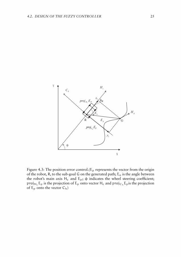
There are several parameters of the car-like robot to take into account (Fig-ure 4.3.): (xc,yc) is the coordinate of point R which is located in the middleof the rear wheels. θc is the heading of the vehicle, i.e., the angle between themain axis Hc of vehicle and the x axis. φ indicates the steering angle of thefront wheels. V represents the velocity of the reference point R measured alongthe main axis of the vehicle.

In the non-holonomic system the angular velocity is dictated by the robotsforward velocity. In this thesis, we constrained the maximum angular velocityto (k · Velc) where Velc represents current linear speed and k represents acoefficient reflect to the curvature of current path.

Input variables

* Eo: an input variable that indicates the angle between the robot’s mainaxis Hc and the vector Ep. It is associated with a five term set of fuzzysets defined over the [−π,π] range that indicates the relative heading to-ward the desired position G point: FrontLeft(FL), SideLeft(SL), Ahead(A),FrontRight(FR), SideRight(SR).

* |Ep|: an input variable that indicates the distance between robot currentposition and desired position. It is associated with a two term set of fuzzysets defined over the [0, |EPMax|] range: Close, Far.

The orientation error Eo is calculated by a two-argument function atan2,

Eo = arctan 2(y1, x1) (4.6)


f

q

R G

Y

X

pE

cH

gH

hC

PH Eprojc

PC Eprojh

oE

1x

1y

Figure 4.3: The position error control.(Ep represents the vector from the originof the robot, R, to the sub-goalG on the generated path; Eo is the angle betweenthe robot’s main axis Hc and Ep; φ indicates the wheel steering coefficient;projHc

Ep is the projection of Ep onto vector Hc and projChEpis the projection

of Ep onto the vector Ch)


where y1 = sgn(Ep · Ch)|projChEp| and x1 = sgn(Ep · Hc)|projHc

Ep|,arctan 2 function is available to distinguish angles come from four quadrants.

The projection of Ep onto Hc is given by,

projHcEp =

Hc · Ep

|Hc|2Hc (4.7)

where projHcEp is the heading vector of robot, Hc · Ep is the dot product,

and the length of the projection is,

|projHcEp| =

|Hc · Ep|

|Hc|(4.8)

The projection of Ep ontoCh that is perpendicular toHc is given by projChEp.

It indicates the sideways vector of the robot.

Output variables

* φ: an output variable which represents the wheel steering coefficient. It isassociated with a five term set of fuzzy sets defined over the [−1, 1] range:LeftLow(LL), LeftHigh(LH), Zero(Z), RightLow(RL), RightHigh(RH).

* V: an output variable which represents the velocity coefficient of the ref-erence point R measured along Hc. It is associated with a two term set offuzzy sets defined over the [0, 1] range: Slow , Fast.

The fuzzy reasoning rules used for modifying position error are presentedas:

* IF Eo is FL THEN φ is LL.

* IF Eo is SL THEN φ is LH.

* IF Eo is A THEN φ is Z.

* IF Eo is FR THEN φ is RL.

* IF Eo is SR THEN φ is RH.

* IF |Ep| is Close THEN V is Slow.

* IF |Ep| is Far THEN V is Fast.


f

RG

Y

X

cH

hC

iq

2x

2y

cq

foE

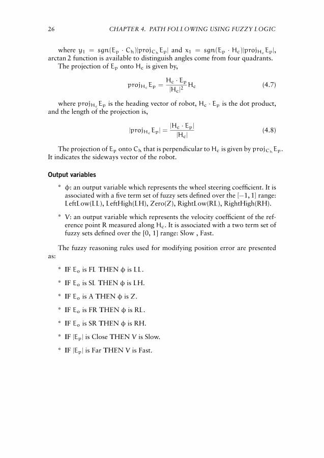
Figure 4.4: The orientation error parameters.(Efo is the angle between sub-goalorientation θi and robot’s main axis Hc; θc is the heading of the vehicle; Efo iscalculated by θi − θc)


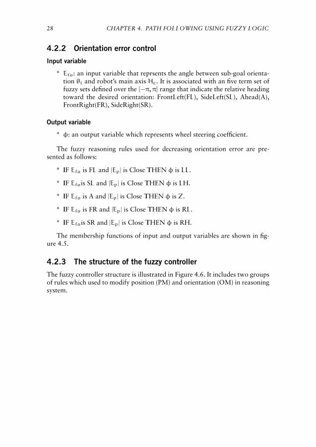
4.2.2 Orientation error control

Input variable

* Efo: an input variable that reprsents the angle between sub-goal orienta-tion θi and robot’s main axis Hc. It is associated with an five term set offuzzy sets defined over the [−π,π] range that indicate the relative headingtoward the desired orientation: FrontLeft(FL), SideLeft(SL), Ahead(A),FrontRight(FR), SideRight(SR).

Output variable

* φ: an output variable which represents wheel steering coefficient.

The fuzzy reasoning rules used for decreasing orientation error are pre-sented as follows:

* IF Efo is FL and |Ep| is Close THEN φ is LL.

* IF Efois SL and |Ep| is Close THEN φ is LH.

* IF Efo is A and |Ep| is Close THEN φ is Z.

* IF Efo is FR and |Ep| is Close THEN φ is RL.

* IF Efois SR and |Ep| is Close THEN φ is RH.

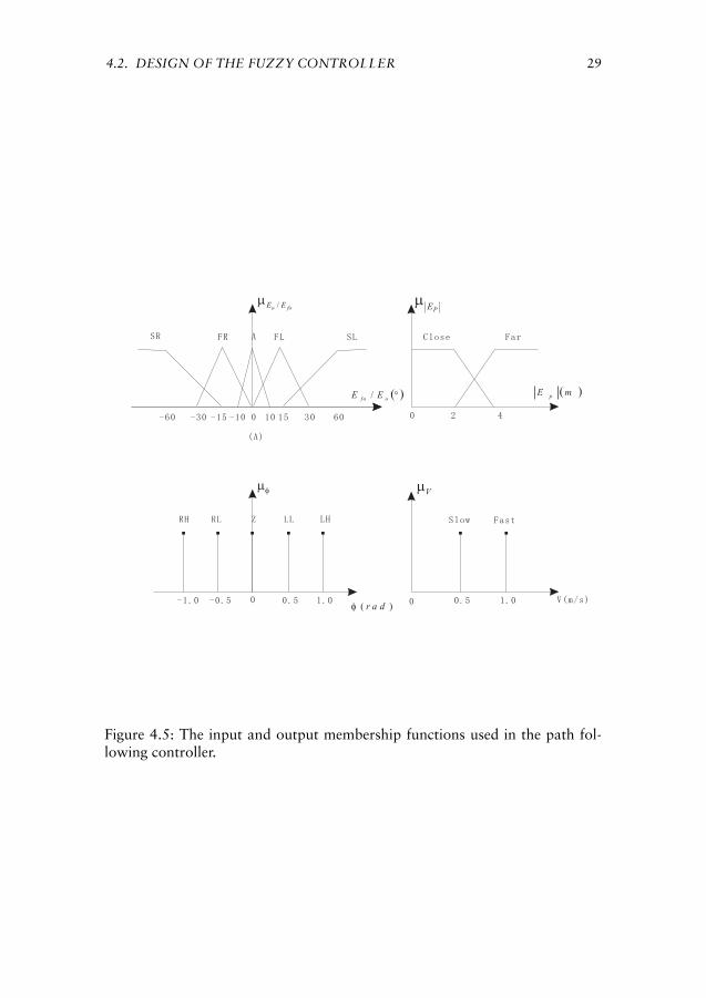
The membership functions of input and output variables are shown in fig-ure 4.5.

4.2.3 The structure of the fuzzy controller

The fuzzy controller structure is illustrated in Figure 4.6. It includes two groupsof rules which used to modify position (PM) and orientation (OM) in reasoningsystem.


0-30-60 -10 10 15 30-15 60 0 2 4

0 0-1.0 -0.5 0.5 1.0 0.5 1.0

( )°ofo EE /

foo EE /m

)( r a df

fm

( )mE p

PEm

V(m/s)

Vm

FR ASR FL SL Close Far

Slow FastRH RL Z LL LH

(A)

Figure 4.5: The input and output membership functions used in the path fol-lowing controller.


PM

oE

OM

foE

pEV

1f

2f

f

Fuzzy controller

Figure 4.6: The structure of the fuzzy controllers.

Chapter 5Experiments and evaluation

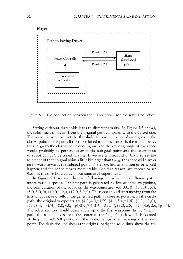
We develop a Player driver to implement our controller. Player is a networksever for robot control. It contains various drivers, which have different func-tions such as path panning and localization for robots. Drivers can send andreceive information from Player by interfaces. Interfaces specify the Player syn-tax and semantics of how the drivers and Player interact. In this Player, “pathfollowing driver” is applied to control a simulated robot to follow continu-ous path. The driver supports the position2D interface in order to read newpositions for the robot’s motors. The driver is written in C++ language andrunning in Ubuntu8.04. The structure of the Player is shown in Figure 5.1. Themost important part of path following driver is the fuzzy controller, it directlycommunicates with Stage to control the similated robot.

We used the 2D robot simulator Stage(version3.0.1) to simulate our robot.Stage is a plugin for Player. It receives instructions from Player and moves asimulated robot in a simulated world. In this test, simple positioning is imple-mented on a car-like kinematic model. The size of robot is [0.44, 0.33], and thesize of the built map is [30, 30] in meters.

5.1 Implementation

As mentioned before in chapter 4.1, a constant threshold value is used to choosethe sub-goal points on the generated path. For a car-like robot, the minimumradius of turning is given by equation (5.1), and all the points inside the circle,that passes by the (x,y) coordinates of the robot and whose radius is rmin, arenot accessible directly using just one combination of translation and rotationvelocities. Therefore, to choose a goal point on the path, we fix the thresholdof distance between the robot and that point to be at least rmin.

rmin =l

tan(φmax)(5.1)

31

32 CHAPTER 5. EXPERIMENTS AND EVALUATION

Stage

simulated

robot

Position2d

Position2d

Fuzzy Controller

Smooth-path

generator

Path following Driver

Player

Figure 5.1: The connection between the Player driver and the simulated robot.

Setting different thresholds leads to different results. As Figure 5.2 shows,the solid track is not far from the original path compares with the dotted one.The reason is when we set the threshold to zero,the robot always goes to theclosest point on the path. If the robot failed to follow the path, the robot alwaystries to go to the closest point once again, and the steering angle of the robotwould probably be perpendicular to the sub-goal point and the orientationof robot couldn’t be tuned in time. If we use a threshold of 0.5m to set thetolerance of the sub-goal point a little bit larger than rmin, the robot will alwaysgo forward towards the subgoal point. Therefore, less orientation error wouldhappen and the robot moves more stable. For that reason, we choose to set0.5m as the threshold value in our simulated experiments.

In Figure 5.3, we test the path following controller with different pathsunder various speeds. The first path is generated by five oriented waypoints,the configuration of the robot on the waypoints are (4.0, 3.0, 0), (6.0, 4.0, 0),(8.0, 3.0, 0), (10.0, 4.0, ), (12.0, 3.0, 0). The robot should start moving from thefirst waypoint and follow the generated path as close as possible. In the circlepath, the original waypoints are (4.0, 4.0,pi/2), (4.6, 5.4,pi/4), (6.0, 6.0, 0),(7.4, 5.4, −pi/4), (8.0, 4.0, −pi/2), (7.4, 2.6, −3pi/4), (6.0, 2.0, −pi), (4.6, 2.6, 3pi/4).The robot motion should begin and stop at the first waypoint. In the "eight"path, the robot moves from the center of the "eight" path which is locatedat the point (4.0, 6.0,pi/4), and the motion stops when arriving at the startpoint. The dash-dot line shows the original path; the solid lines show the tri-

5.1. IMPLEMENTATION 33

4 5 6 7 8 9 10 11 12 13

2.6

2.8

3

3.2

3.4

3.6

3.8

4

4.2

4.4

original paththreshold=0threshold=0.5

Figure 5.2: The results under different thresholds.The dash-dot line representsthe path generated by the given waypoints. The solid line is the track followedby the simulated robot by setting distance threshold to 0.5m while the dottedline is obtained by setting the threshold to 0m


als of path following motions with different speeds, they are 1.0m/s, 2.0m/s,3.0m/s respectively.

5.2 Newton-Rhapson method

For evaluating the results of the proposed path following controller, we ana-lyze the performance of the controller by looking at the errors in position andorientation of the robot with respect to the original path. This means that wehave to find for each point of the resulting path (the trace of the position ofthe robot) the reference point on the original path. In this thesis, we try tocompare the position of the robot with the closest point on the original path.For this matter, we follow two steps: First, we get a rough guess of the closestpoint. Second, we refine the guess with the Newton- Rhapson method appliedto a function that gives the distance from the robot to a point evaluated onthe path. Newton-Rhapson is a method for finding continuous better approx-imations to the zeroes of a real-valued function [28]. The idea of the methodis to use one initial guess which is close to the true root, get the tangent lineof this point and calculate the x-intercept. Then this x-intercept is treated as abetter approximation of the function root and the method is iterated until theaccurate value is found. The iteration function is

xn+1 = xn −f(xn)

f ′(xn)(5.2)

Here we use Newton-Rhapson to solve the minimization problem. In otherwords, we are searching for the minimum of a point to spline distance function.When the derivative is zero, the function is at minimum or maximum value. Theiteration becomes,

Gn+1 = Gn −f ′(Gn)

f ′′(Gn)(5.3)

In my work, the initial guess is determined by detecting the distance betweenthe current position and each point on the original path (the quantity of thepoints on the original path depend on the B-spline parameter increment). Thedistance function in this case is given by

Gt =

√(xi(t) − xr)2 + (yi(t) − yr)2, 0 6 t 6 1, 0 6 i 6 m (5.4)

where i is the index of the spline segments, (xi,yi) are the points of the splinein segment i, (xr,yr) is the poistion of the robot.

We take the point with shortest distance as the initial guess. Since it is hardto calculate the derivative of the distance function, we approximate the deriva-tive by calculating the average value of two slopes of nearby points. In Fig-ure 5.4, we sample two additional points, one before and one after the initialpoint G0 along the spline as G0 + α and G0 − α, the distance from each of the

5.2. NEWTON-RHAPSON METHOD 35

2 4 6 8 10 122

4

6

8

10

12

2 4 6 8

2

4

6

8

2 4 6 8 102

4

6

8

10

Original pathv=1.0m/s

(a) Path following by setting speed to 1.0m/s

2 4 6 8 10 122

4

6

8

10

12

2 4 6 8

2

4

6

8

2 4 6 8 102

4

6

8

10


(b) Path following by setting speed to 2.0m/s

2 4 6 8 10 122

4

6

8

10

12

2 4 6 8

2

4

6

8

2 4 6 8 102

4

6

8

10


(c) Path following by setting speed to 3.0m/s

Figure 5.3: The Results of path following by setting different speeds


R

0G

X

Y

G

)( 0Gf

)(Gf

)( 0 a+Gf)( 0 a-Gf

a-0Ga+0G

Figure 5.4: Using Newton-Rhapson method to find the closest point on thepath to the robot.(f(Gn) is a function that represents the distances between therobot and the points on the path;G0 is a rough guess of the closest point; G0 +αand G0 − α are two nearby points of G0 where α is a small vector.)

three points to current position is easy to calculate. Then we calculate f ′(G0)by,

f ′1(G0) =f(G0 + α) − f(G0)

|α|

f ′2(G0) =f(G0) − f(G0 − α)

|α|

f ′(G0) =f ′1(G0) + f ′2(G0)

2

(5.5)

we calculate f ′′(G0) by,

f ′′(G0) =f ′1(G0) − f ′2(G0)

|α|(5.6)

Finally, we implement Newton-Rhapson method to get the next initial guess.We run this process 10 times to approach the acceptable point.

5.3 Position errors and orientation errors analyze

Figure 5.5 shows the position errors for the different paths. The errors periodi-cally oscillate up and down around an average value. The sharper the curvatureis, the bigger the position error is. From the three figures above, we can see thatunder different speeds, the cycles and trends of error variation are similar. The

5.3. POSITION ERRORS AND ORIENTATION ERRORS ANALYZE 37

0 2 4 6 8 10 12 14 16 18 200

0.05

0.1

0.15

0.2

0.25

0.3

0.35

t(s)

y(m

)

Position errors of wave path following

v=1.0m/sv=2.0m/sv=3.0m/s

(a)

0 5 10 15 20 25 300

0.01

0.02

0.03

0.04

0.05

0.06

0.07

0.08

0.09

t(s)

y(m

)

Position errors of circle path following

v=1.0m/sv=2.0m/sv=3.0m/s

(b)

0 5 10 15 20 25 30 35 40 450

0.05

0.1

0.15

0.2

0.25

t(s)

y(m

)

Position errors of "eight" path following

v=1.0m/sv=2.0m/sv=3.0m/s

(c)

Figure 5.5: The position errors under different speeds for three types of paths,where the x axis represents time in seconts.


Errors Avg(Ep(m)) Avg(Eo(rad))Speed 1.0m/s 2.0m/s 3.0m/s 1.0m/s 2.0m/s 3.0m/s

Wave path 0.1058 0.1132 0.1320 0.3529 0.3587 0.3695Circle path 0.0441 0.0547 0.0630 0.2427 0.2302 0.2179

"Eight" path 0.0609 0.0703 0.0827 0.2516 0.2386 0.2233

Table 5.1: The average position and orientation errors of the different pathsunder different speeds.

maximum error of three paths is lower than 0.26m. It proves that the robotfollows the paths in good way.

Figure 5.6 shows the orientation errors between the robot and the closestpoint on the path for each sampling time increment(x axis indicates the changeof the time). In the Figure 5.6a, the dotted line represents the orientation errorsthat fluctuates from 0 to 1 (rad) during 19.5 seconds with speed 1.0m/s, thesolid line shows the orientation errors oscillated between 0 and 0.9 (rad) during10.0 seconds with speed 2.0m/s, The fluctuation of the dashed line is below0.7 radian during 7.0 seconds. From Figure 5.6b and 5.6c, we can find thatthe range of the three different types of lines are even more closer to eachother comparing with Figure 5.6a. The orientation variation is close to eachother under different speeds. These oscillations seem to happen when the splinecurvature is big. Since both position and orientation errors are oscillating in areasonable area, the path following driver is working fairly well.

It is clear that these results can be improved by tuning the fuzzy rules, andmaybe adding more rules to have a finer coverage of the errors in distance andorientation.

The table below indicates the average position and orientation errors underdifferent speeds for three types of path.

5.3. POSITION ERRORS AND ORIENTATION ERRORS ANALYZE 39

0 2 4 6 8 10 12 14 16 18 200

0.1

0.2

0.3

0.4

0.5

0.6

0.7

0.8

0.9

1

t(s)

y(ra

d)

Orientation errors of wave path following

v=1.0m/sv=2.0m/sv=3.0m/s

(a)

0 5 10 15 20 25 300.05

0.1

0.15

0.2

0.25

0.3

0.35

0.4

t(s)

y(ra

d)

Orientation errors of circle path following

v=1.0m/sv=2.0m/sv=3.0m/s

(b)

0 5 10 15 20 25 30 35 40 450

0.1

0.2

0.3

0.4

0.5

0.6

0.7

0.8

0.9

t(s)

y(ra

d)

Orientation errors of "eight" path following

v=1.0m/sv=2.0m/sv=3.0m/s

(c)

Figure 5.6: The orientation errors under different speeds for three types ofpaths, where the x axis represents time in seconts.

Chapter 6Conclusions

6.1 Summary

This thesis has presented an implementation of a fuzzy-logic-based controllerfor following continuous paths. The controller was implemented a simulatedrobot through the robot middle ware "Player". The result of the simulationexperiments show that with a minimal set of rules, it is possible to get an ac-ceptable path following behavior.

The thesis has also presented a way of generating continuous path from aset of oriented waypoints. Such paths were generated using uniform cubic B-splines, which are a flexible tool used for geometric modeling. The generationof the B-splines takes into account possible collisions with nearby obstacles aswell as the kinematic constraints of the vehicle that is intended to follow thecontinuous path. Additional control points are added along the orientation ofcontrol points, by moving these additional points away or towards the way-points, the curvature of spline is modified to fulfill the steering constrain ofcar-like robot and to avoid the static obstacles.

6.2 Further work

The work presented in this thesis can be considered as an initial step towardsrealizing a robust path-following controller for car-like robots. Therefore, theseare many possible other steps that can be taken to improve our controller.

Firstly, the controller can be extended to react to moving and static objectsby adding more behaviors for that matter.

Secondly, one can improve the controller by considering more rules thatcover different situations of how the robot pose is with respect to the originalpath.

Thirdly, in the thesis we only did experiments to follow paths, a futurework can be testing and tuning the performance of the controller to followtrajectories at different speeds. We expect that the controller to be modified by

41

42 CHAPTER 6. CONCLUSIONS

adding more output sets to be able to cope with the change in the referencepoint of the trajectory.

Another interesting possible future work would be to port and test the con-troller on a real mobile robot.

References

[1] Jacky Baltes and Yuming Lin. Path-tracking control of non-holonomiccar-like robot with reinforcement learning. In Working notes of the IJ-CAI’99 Third International Workshop on Robocup, pages 162–173. IJ-CAI Press, 2000. (Cited on page 10.)

[2] Abdelbaki Bouguerra, Henrik Andreasson, Achim J. Lilienthal, Björn Ås-trand, and Thorsteinn Rögnvaldsson. Malta: A system of multiple au-tonomous trucks for load transportation. In Proceedings of the EuropeanConference on Mobile Robots (ECMR), pages 91–96, 2009. (Cited onpage 1.)

[3] J. Connors and G. H. Elkaim. Manipulating b-spline based paths forobstacle avoidance in autonomous ground vehicles. In ION NationalTechnical Meeting, ION NTM 2007, San Diego, CA, USA, 2007. (Citedon page 6.)

[4] Th. Fraichard and Ph. Garnier. Fuzzy control to drive car-like vehicles.Robotics and Autonomous Systems, 34:1–22, 1997. (Cited on page 11.)

[5] Philippe Garnier, Cyril Novales, and Christian Laugier. An hybrid motioncontroller for a real car-like robot evolving in a multi-vehicle environment.Grenoble Cedex, pages 25–26, 1995. (Cited on page 10.)

[6] Brian P. Gerkey, Richard T. Vaughan, and Andrew Howard. Theplayer/stage project: Tools for multi-robot and distributed sensor systems.In In Proceedings of the 11th International Conference on AdvancedRobotics, pages 317–323, 2003. (Cited on page 3.)

[7] F. Gómez-Bravo, F. Cuesta, A. Ollero, and A. Viguria. Continuous curva-ture path generation based on b-spline curves for parking manoeuvres.Robot. Auton. Syst., 56(4):360–372, April 2008. (Cited on pages 5and 16.)

43

44 REFERENCES

[8] Dongbing Gu and Huosheng Hu. Neural predictive control for a car-like mobile robot. International Journal of Robotics and AutonomousSystems, 39:73–86, 2002. (Cited on pages 8 and 9.)

[9] Kale Harbick, James F. Montgomery, and Gaurav S. Sukhatme. Planarspline trajectory following for an autonomous helicopter. In in IEEE In-ternational Symposium on Computational Intelligence in Robotics andAutomation, pages 237–242, 2001. (Cited on page 7.)

[10] Matthias Hentschel, Oliver Wulf, and Bernardo Wagner. A hybrid feed-back controller for car-like robots - combining reactive obstacle avoidanceand global replanning. Integr. Comput.-Aided Eng., 14(1):3–14, January2007. (Cited on page 10.)

[11] J. H. Hwang, R. C. Arkin, and D. S. Kwon. Mobile robots at your fin-gertip: Bezier curve on-line trajectory generation for supervisory control.In Proceedings of the IEEE/RSJ International Conference on IntelligentRobots and Systems, 2003. (Cited on page 6.)

[12] Jyh-Shing Roger Jang and Chuen-Tsai Sun. Neuro-fuzzy and soft com-puting: a computational approach to learning and machine intelligence.Prentice-Hall, Inc., Upper Saddle River, NJ, USA, 1997. (Cited on pages12, 13, and 23.)

[13] Eric Larsen, Stefan Gottschalk, Ming C. Lin, and Dinesh Manocha. Fastproximity queries with swept sphere volumes. Technical report, 1999.(Cited on page 19.)

[14] Alessandro De Luca, Giuseppe Oriolo, Alessandro De, and Claude Sam-son. Feedback control of a nonholonomic car-like robot, 1997. (Citedon page 8.)

[15] Julio E. Normey-Rico, Ismael Alcalá, Juan Gómez-Ortega, and Eduardo F.Camacho". Mobile robot path tracking using a robust pid controller.Control Engineering Practice, 9(11):1209 – 1214, 2001. (Cited on page8.)

[16] Fares Boudjema Noureddine Ouadah, Lamine Ourak. Car-like mobilerobot oriented positioning by fuzzy controllers. volume 5, 2008. (Citedon page 11.)

[17] P Venkata Subba Reddy. Fuzzy modeling and natural language processingfor paninis sanskrit grammar. Journal of Computer Science and Engineer-ing, 1(1):99–101, 2010. (Cited on page 10.)

[18] Eric Ronco and Peter J. Gawthrop. Neural networks for modelling andcontrol. Technical report, 1997. (Cited on page 8.)

REFERENCES 45

[19] M. Gloria Sánchez-Torrubia, Carmen Torres-Blanc, and Sanjay Krish-nankutty. Mamdani’s fuzzy inference emathteacher: a tutorial for activelearning. W. Trans. on Comp., 7(5):363–374, May 2008. (Cited on page13.)

[20] Dong Hun Shin and Sanjiv Singh. Path generation for robot vehicles us-ing composite clothoid segments. Technical Report CMU-RI-TR-90-31,Robotics Institute, Pittsburgh, PA, December 1990. (Cited on page 6.)

[21] M. Sugeno and G. T. Kang. Structure identification of fuzzy model. FuzzySets Syst., 28(1):15–33, October 1988. (Cited on pages 13 and 22.)

[22] R.S. Sutton and A.G. Barto. Reinforcement Learning: An Introduction.Adaptive Computation and Machine Learning. Mit Press, 1998. (Citedon page 9.)

[23] B. Triggs. Motion planning for nonholonomic vehicles: An introduction.Jun. 1993. (Cited on page 2.)

[24] Petr Wagner, Jiri Kotzian, Jan Kordas, and Viktor Michna. Path planningand tracking for robots based on cubic hermite splines in real-time. InETFA, pages 1–8, 2010. (Cited on page 6.)

[25] Jiajun Wang. Nonlinear control strategies research of nonholonomic con-trol systems. Sep. 2010. (Cited on page 2.)

[26] Lee Weiss, Arthur C Sanderson, and C.P. Neuman. Dynamic visual servocontrol of robots: An adaptive image-based approach. In Proceedings ofthe 1985 IEEE International Conference on Robotics and Automation(ICRA ’85), volume 2, pages 662 – 668, March 1985. (Cited on page 8.)

[27] T. Yamakawa. Stablization of an inverted pendulum by a high-speedfuzzy logic controller hardware system. Fuzzy Sets Syst., 32(2):161–180,September 1989. (Cited on page 10.)

[28] Tjalling J. Ypma. Historical development of the newton-raphson method.SIAM Rev., 37(4):531–551, December 1995. (Cited on page 34.)

[29] L. Zadeh. The concept of a linguistic variable and its application to ap-proximate reasoning. Information Sciences, 8(3):199–249, 1975. (Citedon pages 10 and 11.)

[30] Lavi M. Zamstein. Koolio: Path planning using reinforcement learningon a real robot platform. In University of Florida, pages 25–26, 2006.(Cited on page 10.)

[31] Ali Zilouchian and Mohammad Jamshidi, editors. Intelligent Control Sys-tems Using Soft Computing Methodologies. CRC Press, Inc., Boca Raton,FL, USA, 1st edition, 2000. (Cited on page 2.)

path following for a car-like mobile robot based on fuzzy-logic

Documents