path integral methods for parabolic partial differential ... · pdf filethe mathematica®...

The Mathematica® Journal

Path Integral Methods for Parabolic Partial Differential Equations With Examples from Computational Finance

Andrew LyasoffBy using specific examples—mostly from computational finance—thispaper shows that Mathematica is capable of transforming Feynman-typeintegrals on the pathspace into powerful numerical procedures for solvinggeneral partial differential equations (PDEs) of parabolic type, with bound-ary conditions prescribed at some fixed or free time boundary. Comparedto the widely used finite difference methods, such procedures are moreuniversal, are considerably easier to implement, and do not require anymanipulation of the PDE. An economist or a financial engineer who workswith very general models for asset values, including the so-called stochas-tic volatility models, will find that this method is just as easy to work withas the classical Black–Scholes model, in which asset values can follow onlya geometric Brownian motion process.

‡ 1. IntroductionParabolic partial differential equations (PDEs), of which the standard heatequation is a special case, are instrumental for many applications in physics,engineering, economics, finance, weather forecasting, and many other fields. Inpractice, the solution to most parabolic PDEs can be computed only approxi-mately by way of some special numerical procedure. Currently, in most if not allpractical implementations, this procedure happens to be some variation of thewell-known finite difference method.

This method involves tools and terminology that are familiar to most specialistsin numerical methods. Its underlying principle is relatively easy to understand: itcomes down to solving sequentially a very large number of linear systems.Unfortunately, in most applications

The Mathematica Journal 9:2 © 2004 Wolfram Media, Inc.

Unfortunately, in most applications the size of each system is overwhelming andthe practical implementation of the method is not straightforward, especially inthe case of non-constant coefficients.

It has been well known for nearly as long as the finite difference method hasbeen in existence that the solution of the heat equation can be expressed as a pathintegral (also known as a Feynman integral). For a mathematician, this is nothingbut an expected value relative to Wiener’s probability distribution on the spaceof sample paths. This construction also admits a generalization: the solution of afairly general parabolic PDE can be expressed as an expected value (alias: aFeynman integral) relative to a special probability distribution on the pathspace(alias: the Wiener measure). Although possible in principle, the numericalcalculation of path integrals has always been seen as a formidable task and arather inefficient way to produce a solution to a parabolic PDE. As the examplesincluded in this article demonstrate, not only is this no longer the case, but, withthe advent of Mathematica 4, the solution to a rather general parabolic PDE canbe produced by merely expressing the associated path integral in Mathematica.

The method developed in this paper is a good illustration of the way in whichsignificant new developments in the common man’s computing tools transformthe type of mathematics that is commonly perceived as interesting and impor-tant. We will show with concrete examples (see Section 4 below) that computingthe price of an European call option—a classical problem in computationalfinance—in terms of path integrals is just as easy, just as accurate, and virtuallyjust as fast as calculating the price directly by using the Black–Scholes formula. Inother words, for all practical purposes, the path integral representation of thesolution of the Black–Scholes PDE in Mathematica is just as good as a closedform solution. Unlike the true closed form solution, however, the path integralrepresentation can be used with any reasonably behaved payoff. Of course, thisapproach would have been unthinkable when Black and Scholes developed theirmethod [1]. Their calculation was interesting and profoundly important,although the really important discovery that they made was the principle that ledto the Black–Scholes PDE—not the Black–Scholes formula, as is commonlybelieved.

It is remarkable how Mathematica’s ability to combine advanced symbolic comput-ing with advanced numerical procedures can turn a fairly abstract mathematicalconcept (in this case, integration on the pathspace) into a rather practical comput-ing tool. This brings a method to consumers of computing technology that isboth universal and “smart,” in the sense that it is capable of taking advantage ofthe structure of the PDE. For example, the method will need fewer iterations ifthe coefficients are close to linear, and can work on a very coarse grid in the statespace if the solution is reasonably close to a polynomial. Above all, its implementa-tion is extremely straightforward, involves very little programming, and does notrequire any knowledge of sophisticated numerical methods, which Mathematicauses implicitly. For a financial engineer, this means that pricing an option withany reasonably-behaved payoff function on an asset that follows a rather generaltime-homogeneous Markov process, including options that allow early exercise,would be just as easy as pricing a vanilla European call or put option on an assetthat follows a standard geometric Brownian motion process. Such technologycan have a considerable impact on the financial industry. Indeed, it has long beenrecognized that actual stock prices exhibit self-regulatory patterns that areinconsistent with the properties of the geometric Brownian motion. Yet theBlack–Scholes model remains immensely popular mainly because, with thecurrent level of widely available computing technology, any other model wouldbe virtually intractable for an average practitioner.

400 Andrew Lyasoff


It is remarkable how Mathematica’s ability to combine advanced symbolic comput-ing with advanced numerical procedures can turn a fairly abstract mathematicalconcept (in this case, integration on the pathspace) into a rather practical comput-ing tool. This brings a method to consumers of computing technology that isboth universal and “smart,” in the sense that it is capable of taking advantage ofthe structure of the PDE. For example, the method will need fewer iterations ifthe coefficients are close to linear, and can work on a very coarse grid in the statespace if the solution is reasonably close to a polynomial. Above all, its implementa-tion is extremely straightforward, involves very little programming, and does notrequire any knowledge of sophisticated numerical methods, which Mathematicauses implicitly. For a financial engineer, this means that pricing an option withany reasonably-behaved payoff function on an asset that follows a rather generaltime-homogeneous Markov process, including options that allow early exercise,would be just as easy as pricing a vanilla European call or put option on an assetthat follows a standard geometric Brownian motion process. Such technologycan have a considerable impact on the financial industry. Indeed, it has long beenrecognized that actual stock prices exhibit self-regulatory patterns that areinconsistent with the properties of the geometric Brownian motion. Yet theBlack–Scholes model remains immensely popular mainly because, with thecurrent level of widely available computing technology, any other model wouldbe virtually intractable for an average practitioner.

Finding the most efficient way to present the computational aspects of the pathintegral method and its implementation in Mathematica is a bit of a challenge.Indeed, on the one hand, specialists in (and consumers of) numerical methods forPDEs do not usually speak the language of path integrals. On the other hand,specialists in mathematical physics and probability, who do speak the language ofpath integrals, are not usually interested in numerical methods and computerprogramming. This article grew out of the desire to meet this challenge. In spiteof its use of high-end mathematical jargon, it is mainly about Mathematica andthe impact that Mathematica can make not only on the way in which importantcomputational problems are being solved, but also on our understanding ofwhich mathematical methods are “applied” and which are “theoretical.”

Note about the notation: Following the common convention in Mathematica,in all equations and algebraic expressions, arguments of functions are wrappedwith square brackets and parenthesis are used only for grouping. Double-strucksquare brackets are used to denote intervals: open intervals are denoted as T a, bPand closed intervals are denoted as Pa, bT.

For the purpose of illustration, all time-consuming operations in this notebookare followed by //Timing. The CPU times reflect the speed of a 2.8GhzIntel® Pentium® 4 processor with 768MB of RAM running Mathematica 5.0.

‡ 2. Some Background: Solutions to Second-order Parabolic Partial Differential Equations as Path IntegralsThis section outlines some well-known principles and relations on which themethod developed in this paper is based. A complete, detailed, and rigorousdescription of these principles can be found in the ground-breaking work ofStroock and Varadhan [2] and also in [3, 4]. The computational aspects of themethods developed in these works have not been explored fully, and to a largeextent the present work is a modest attempt to fill this gap.

The Feynman integral of a real function f @D defined on the space !0 Pt, TT, whichconsists of continuous sample paths w : Pt, T T # ! with the property wt = 0, canbe expressed as the following formal expression

(2.1)‡8w œ !0 Pt,TT < f @wD ‰- 1ÅÅÅÅÅ2 ŸtT I „wsÅÅÅÅÅÅÅÅÅÅÅÅ„s M2

„s ikjjjj ÂsœPt,TT „ ws

ÅÅÅÅÅÅÅÅÅÅÅÅÅÅÅÅÅÅÅè!!!!!!!2 p

y{zzzz ,

Path Integral Methods for Parabolic Partial Differential Equations 401


which is understood as the limit of the following sequence of multiple integrals

(2.2)H2 pL- kÅÅÅÅÅ2 ‡!

… ‡!

fk @w0 , wd , …, wkd D ‰-„

i=1

k Iwi d -wHi-1L d M2ÅÅÅÅÅÅÅÅÅÅÅÅÅÅÅÅÅÅÅÅÅÅÅÅÅÅÅÅÅÅÅÅÅÅÅÅÅÅÅÅÅÅÅÅÅ2 d

µ „ Hwd - w0 L … „ Hwkd - wHk-1L d L,where kr1, d := T -tÅÅÅÅÅÅÅÅÅÅÅk and fk @w0 , wd , …, wkd D is the result of the evaluation of f @Dat the piecewise linear sample path from the space !0 Pt, T T, whose values at thepoints t + id, 0 b i b k, are given by the vector Hw0 , wd , …, wkd L. It would not bean exaggeration to say that the convergence of the sequence in (2.2)—andtherefore the fact that the integral in (2.1) is meaningful—is a miracle, withoutwhich very little of what we currently know about the universe would have takenplace. Indeed, “miracle” is the only term that can explain the fact that, as waspointed out in [4], the infinities that arise under the exponent in (2.1) not onlyoffset the infinities that arise under the product sign, but also offset them in sucha way that the result is a perfectly well defined and highly nontrivial probabilitymeasure on the space !0 Pt, T T, known as the Wiener measure. Not only is theintegral in (2.1) the perfectly meaningful “expected value of f @D,” but when f @D isgiven by f @wD := L@x + wT D, w œ !0 Pt, TT, for some fixed x œ ! and somereasonably behaved function L : ! # !, then, as a function of x and t, thisexpected value coincides with the solution of the standard heat equation

(2.3)∑t u@t, xD + " u@t, xD = 0 , " :=1ÅÅÅÅÅÅ2

∑x,x , x œ ! , t b T ,

with boundary condition u@T , xD ª L@xD. In fact, this statement admits a generali-zation: if " is replaced by a general elliptic differential operator of the form

(2.4)" =1ÅÅÅÅÅÅ2

s2 @xD ∑x,x +a@xD ∑x ,

assuming that the coefficients s@D and a@D are reasonably behaved, the solution ofthe boundary value problem (2.3) can still be expressed as a path integral similarto the one in (2.1). The only difference is that in this case the path integral isunderstood as the limit of the sequence

(2.5)‡

!

„ Hwd - xL pd @x, wd D µ ‡!

„ Hw2 d - wd L pd @wd , w2 d Dµ ∫ µ ‡

!

„ Hwkd - wHk-1L d L pd @wHk-1L d , wkd D L@x + wkd D, k r 1 ,

where pt @x, yD is the transition probability density of the Markov process Xt ,t r 0, determined by the stochastic equation

(2.6)„ Xt = s@Xt D „ ßt + a@Xt D „ t,

in which ßt , t r 0, is a given Brownian motion process. In other words,Ht, x, yL ö pt @x, yD is characterized by the fact that for any test function j@D onehas

E@j@Xt+h D » Xt = x D = ‡!

j@yD ph @x, yD „ y.

We will say that the process Xt , t r 0, is a sample path realization of the Markoviansemigroup ‰t " , t r 0, " being the differential operator from (2.4), and will refer tothe transition density Ht, x, yL ö pt @x, yD as the integral kernel of the semigroup‰t" , t r 0. This integral kernel is also known as the fundamental solution of theequation H∑t -"L u@t, xD = 0, that is, a solution which satisfies the initial conditionu@0, xD = d y @xD, where dy @D stands for the usual Dirac delta function with massconcentrated at the point y œ #. This means that, formally, pt @x, yD can beexpressed as pt @x, yD = H‰t" dy L@xD.

402 Andrew Lyasoff


We will say that the process Xt , t r 0, is a sample path realization of the Markoviansemigroup ‰t " , t r 0, " being the differential operator from (2.4), and will refer tothe transition density Ht, x, yL ö pt @x, yD as the integral kernel of the semigroup‰t" , t r 0. This integral kernel is also known as the fundamental solution of theequation H∑t -"L u@t, xD = 0, that is, a solution which satisfies the initial conditionu@0, xD = d y @xD, where dy @D stands for the usual Dirac delta function with massconcentrated at the point y œ #. This means that, formally, pt @x, yD can beexpressed as pt @x, yD = H‰t" dy [email protected] thorough exploration of this generalization of the Feynman integral can befound in the seminal work of Stroock and Varadhan [2]. The terminology issomewhat different from the one used here, that is, instead of “path integrals,” itcomes down to a study of probability distributions on the pathspace associatedwith equations similar to the one in (2.6). Such a framework is much morerigorous and powerful. However, our goal is to develop a numerical procedurethat computes the solution of the PDE in (2.3) as an expected value, and in thisrespect Feynman’s formalism proves to be quite useful.

‡ 3. Path Integrals as Approximation Procedures The multiple integral in (2.5) is actually an iterated integral, which can betranscribed as a recursive rule. More specifically, if for some fixed T r 0, thefunction Ht, xL ö u@t, xD satisfies the equationH∑t +"L u@t, xD = 0 , " ª

1ÅÅÅÅÅÅ2

s2 @xD ∑x,x +a@xD ∑x ,

for t b T and for x œ !, assuming that the map x ö u@T , xD is given, one cancompute the maps x ö u@T - id, xD consecutively for i = 1, 2, …, according tothe following procedure

(3.1)u@T - i d, xD = ‡

!

pd @x, yD µ u@T - Hi - 1L d, yD „ y

= E@u@T - Hi - 1L d, Xd D » X0 = x D , i = 1, 2, ….

As we will soon see, the implementation of this procedure in Mathematica iscompletely straightforward. Since the above identity holds for every choice ofd > 0, this raises the question: why does one need the recursive procedure at all?After all, one can always take d = T - t and then use the recursive rule in (3.1)only for i = 1, which comes down to what is known as the Feynman–Kac formula:

(3.2)u@t, xD = ‡

!

pT -t @x, yD µ u@T , yD „ y ª E@u@T , XT -t D » X0 = x Dª E@L@XT -t D » X0 = x D.

Unfortunately, the integral kernel Ht, x, yL ö pT -t @x, yD ª H‰HT -tL " d y L @xD canonly be expressed in a form that allows one to actually compute this lastintegral—for example, by way of some numerical procedure—for some specialchoice of the coefficients s@D and a@D. The idea, then, is to use the recursive rule(3.1) with some “sufficiently small” d > 0 and hope that for such a choice of d,pd @x, yD can be replaced with some approximate kernel, which, on the one hand,makes the integral (the expected value) on the right side of (3.1) computable and,on the other hand, does not allow the error in the calculation of u@T - i d, xDcaused by this approximation to grow larger than i d oHdL. We will do whatappears to be completely obvious and intuitive: replace s@D and a@D with theirfirst-order Taylor expansions about the point x œ !. Intuitively, it should beclear that when the process Xt , t r 0 is governed by the stochastic equation in(2.6) over a short period of time, its behavior cannot be very different from thebehavior of a process that starts from the same position X0 = x and is governedby the first-order Taylor approximation of the stochastic equation in (2.6)around the point x œ !. The reason why one has to settle for a first-orderapproximation is that, in general, only when the coefficients s@D and a@D in (2.6)are affine functions can one solve this equation explicitly, that is, write thesolution as an explicit function of the driving Brownian motion. In general, theprobability density of this explicit function is not something that is known tomost computing systems and therefore its use in the computation of the integralon the right side of (3.1) is not straightforward. One way around this problem isto compute, once and for all, the transition probability density of a Markovprocess governed by a stochastic differential equation (SDE) with affine coeffi-cients, and then add that function of seven variables (four parameters determinedby the two affine coefficients s@D and a@D plus the variables t, x, and y) to the listof standard functions in the system. In this exposition we will not go that far,however. Instead, we will develop a second level of approximation, in which thesolution of a general SDE with affine coefficients will be replaced by a comput-able function of the starting point x, the time t, and the position of the drivingBrownian motion at time t. After this second level of approximation, the computa-tion of the integral on the right side of (3.1) comes down to computing a Gauss-ian integral, which, as we will soon see, is not only feasible, but is also extremelyeasy to implement. Note that when the coefficients s@D and a@D are linear func-tions, this second level of approximation of the solution of the stochastic equa-tion in (2.6) actually coincides with the exact solution and is therefore redundant.



Unfortunately, the integral kernel Ht, x, yL ö pT -t @x, yD ª H‰HT -tL " d y L @xD canonly be expressed in a form that allows one to actually compute this lastintegral—for example, by way of some numerical procedure—for some specialchoice of the coefficients s@D and a@D. The idea, then, is to use the recursive rule(3.1) with some “sufficiently small” d > 0 and hope that for such a choice of d,pd @x, yD can be replaced with some approximate kernel, which, on the one hand,makes the integral (the expected value) on the right side of (3.1) computable and,on the other hand, does not allow the error in the calculation of u@T - i d, xDcaused by this approximation to grow larger than i d oHdL. We will do whatappears to be completely obvious and intuitive: replace s@D and a@D with theirfirst-order Taylor expansions about the point x œ !. Intuitively, it should beclear that when the process Xt , t r 0 is governed by the stochastic equation in(2.6) over a short period of time, its behavior cannot be very different from thebehavior of a process that starts from the same position X0 = x and is governedby the first-order Taylor approximation of the stochastic equation in (2.6)around the point x œ !. The reason why one has to settle for a first-orderapproximation is that, in general, only when the coefficients s@D and a@D in (2.6)are affine functions can one solve this equation explicitly, that is, write thesolution as an explicit function of the driving Brownian motion. In general, theprobability density of this explicit function is not something that is known tomost computing systems and therefore its use in the computation of the integralon the right side of (3.1) is not straightforward. One way around this problem isto compute, once and for all, the transition probability density of a Markovprocess governed by a stochastic differential equation (SDE) with affine coeffi-cients, and then add that function of seven variables (four parameters determinedby the two affine coefficients s@D and a@D plus the variables t, x, and y) to the listof standard functions in the system. In this exposition we will not go that far,however. Instead, we will develop a second level of approximation, in which thesolution of a general SDE with affine coefficients will be replaced by a comput-able function of the starting point x, the time t, and the position of the drivingBrownian motion at time t. After this second level of approximation, the computa-tion of the integral on the right side of (3.1) comes down to computing a Gauss-ian integral, which, as we will soon see, is not only feasible, but is also extremelyeasy to implement. Note that when the coefficients s@D and a@D are linear func-tions, this second level of approximation of the solution of the stochastic equa-tion in (2.6) actually coincides with the exact solution and is therefore redundant.

Before we can implement the plan that we just outlined, we must address anentirely mundane question: how is each function y öu@T - i d, yD, i r 0, goingto be represented in the computing system? The answer is that we will usepolynomial interpolation; that is, in every iteration, the integral on the right sideof (3.1) (with the approximate integral kernel) will be computed only for

x œ $ := :S + j h

ÅÅÅÅÅÅÅÅm

; -m b j b m>,

where S, h, and m are given parameters. Furthermore, in the actual computationof the integral, the map y öu@T - Hi - 1L d, yD will be replaced by the mapconstructed by way of polynomial interpolation (and extrapolation) from thevalues

uÄÇÅÅÅÅÅÅÅÅT - Hi - 1L d, S + j

hÅÅÅÅÅÅÅÅm

ÉÖÑÑÑÑÑÑÑÑ, -m b j b m.

In other words, our strategy is to store each of the functions u@t, ÿD, fort = T - id, i = 1, 2, …, as a list of 2 m + 1 real values and interpret u@t, ÿD as theresult of polynomial interpolation from that list. This means that we will beconstructing the solution u@t, xD only for x œ PS - h, S + hT and t = T - id,i = 1, 2, …, for some appropriate choice of d > 0. In most practical situations,one needs to construct u@t, ÿD only on some finite interval and only for a fixedt < T . To do this with our method, one must set d = T -tÅÅÅÅÅÅÅÅÅÅÅk for some sufficientlylarge k œ "+ , and then iterate (3.1) k times after choosing S and h so that theinterval of interest is covered by the interval PS - h, S + hT; the number ofinterpolation nodes (2 m + 1) must be chosen so that the polynomial interpola-tion is reasonably accurate. This might appear as a daunting programming task,but, as we will soon see, in Mathematica it involves hardly any programming atall. The reason is that the integration routine can accept as an input the outputfrom the interpolation routine—all in symbolic form. This illustrates perfectlythe point made earlier: new developments in the common man’s computing toolscan change the type of mathematics that one can use in practice.

404 Andrew Lyasoff


In other words, our strategy is to store each of the functions u@t, ÿD, fort = T - id, i = 1, 2, …, as a list of 2 m + 1 real values and interpret u@t, ÿD as theresult of polynomial interpolation from that list. This means that we will beconstructing the solution u@t, xD only for x œ PS - h, S + hT and t = T - id,i = 1, 2, …, for some appropriate choice of d > 0. In most practical situations,one needs to construct u@t, ÿD only on some finite interval and only for a fixedt < T . To do this with our method, one must set d = T -tÅÅÅÅÅÅÅÅÅÅÅk for some sufficientlylarge k œ "+ , and then iterate (3.1) k times after choosing S and h so that theinterval of interest is covered by the interval PS - h, S + hT; the number ofinterpolation nodes (2 m + 1) must be chosen so that the polynomial interpola-tion is reasonably accurate. This might appear as a daunting programming task,but, as we will soon see, in Mathematica it involves hardly any programming atall. The reason is that the integration routine can accept as an input the outputfrom the interpolation routine—all in symbolic form. This illustrates perfectlythe point made earlier: new developments in the common man’s computing toolscan change the type of mathematics that one can use in practice.

A good point can and should be made that approaching (from a purely computa-tional point of view) a general parabolic PDE like the one in (2.3) in the way wedid and with the type of mathematics that we have chosen, namely, integrationon the path space, is more than just natural. Indeed, the connection between thedistribution of the sample paths of the process Xt , t r 0, governed by the stochas-tic equation in (2.6) and the parabolic PDE (2.3) runs very deep (see [2, 3] for adetailed study of this relationship). The point is that the distribution on the spaceof sample paths associated with the SDE (2.6) encodes all the information aboutthe elliptic differential operator " from (2.4) and, therefore, all the informationabout the function

u@t, xD = H‰HT -tL " L L@xD , x œ ! , t b T .

This is analogous to the claim that the integral curves of a vector field encode allthe information about the vector field itself. Actually, this is much more than amere analogy. To see this, notice that if " were a first-order differential operator(i.e., a vector field) in the open interval # Õ !, if t ö Xt were an integral curvefor " starting from X0 = x, and if Ht, xL ö u@t, xD has the propertyH∑t +"L u@t, xD = 0, then one would have

(3.3)u@T , XT -t D - u@t, xD = ‡t

T

∑s u@s, Xs-t D „ s = ‡t

T

0 „ s = 0.

In other words, the integral curves of the vector field " can be characterized as“curves along which any solution of H∑t +"L u@t, xD = 0 remains constant.” This isinteresting as well as quite practical. Indeed, if H∑t +"L u@t, xD = 0 must be solvedfor t b T and x œ # with boundary condition u@T , xD = L@xD, x œ #, one cancompute the solution u@t, xD by first solving the ODE „ÅÅÅÅÅÅÅ„t Xt = "@Xt D with initialdata X0 = x. Here we treat " as a “true” vector field (i.e., as a map of the form" : # # !) and then by evaluating the function L@D (assuming that it is given) atthe point XT -t . Thus, the computation of u@t, xD, for a given x œ # and t < T ,essentially comes down to constructing the integral curve P0, T - tT ú s ö Xsfor the vector field " with initial position X0 = x.



In other words, the integral curves of the vector field " can be characterized as“curves along which any solution of H∑t +"L u@t, xD = 0 remains constant.” This isinteresting as well as quite practical. Indeed, if H∑t +"L u@t, xD = 0 must be solvedfor t b T and x œ # with boundary condition u@T , xD = L@xD, x œ #, one cancompute the solution u@t, xD by first solving the ODE „ÅÅÅÅÅÅÅ„t Xt = "@Xt D with initialdata X0 = x. Here we treat " as a “true” vector field (i.e., as a map of the form" : # # !) and then by evaluating the function L@D (assuming that it is given) atthe point XT -t . Thus, the computation of u@t, xD, for a given x œ # and t < T ,essentially comes down to constructing the integral curve P0, T - tT ú s ö Xsfor the vector field " with initial position X0 = x.

Of course, the remark just made can be found in any primer on PDEs anddemonstrates how natural our approach to parabolic PDEs actually is. Indeed,the Feynman–Kac formula in (3.2) is essentially an analog of the relation in (3.3)in the case where " is a second-order differential operator of elliptic type. Thisamounts to the claim that the solution of the parabolic PDE H∑t +"L u@t, xD = 0remains constant on average along the sample path of the process Xt , t r 0, whichis exactly the sample path representation of the semigroup ‰t" , t r 0. Clearly, forany given starting point X0 = x, the probability distribution of the sample path ofthe process Xt , t r 0, has the meaning of a “distributed integral curve” for thesecond-order differential operator ". This interpretation of the Feynman–Kacformalism is due to Stroock [3] and has been known for quite some time. Theonly “novelty” here is our attempt to utilize its computing power. The recursiverule (3.1) is analogous to a numerical procedure for constructing an integralcurve of a standard (first-order) vector field by solving numerically a first-orderordinary differential equation.

One should point out that the main concept on which all finite difference meth-ods rest is quite natural, too. Indeed, the intrinsic meaning of a partial derivativeis nothing but “a difference quotient of infinitesimally small increments.” How-ever, such a concept is intrinsic in general and not necessarily intrinsic for theequation H∑t +"L u@t, xD = 0. This is very similar to encoding an image of a circleas a list of a few thousand black or white pixels. There are various methods thatwould allow one to compress such an image, but they all miss the main point: acircle is determined only by its radius and center point, and this is the only datathat one actually needs to encode. It is not surprising that, in order to achieve areasonable accuracy, essentially all reincarnations of the finite difference methodrequire a very dense grid on the time scale as well as the state-space.

As was pointed out earlier, path integrals can be used just as easily in the case offree boundary value problems of the following type: given an interval # Õ ! anda number T œ !+ , find a function T - ¶, T T ä # ú Ht, xL ö u@t, xD œ ! and alsoa free time-boundary T - ¶, T T ú t ö x* @tD œ # so that

(3.4)

1L u@t, xD r L@xD, for x œ # ;

2L u@t, xD = L@xD, for x œ # › T - ¶, x* @tDT ;

3L H∑t +"L u@t, xD = 0, for x œ # › T x* @tD, ¶P;

4L limx äx* @tD u@t, xD = L@x* @tDD and H∑x uL@t, x* @tDD = L£ @x* @tDD;5L u@T , xD = L@xD for x œ #.

This is an optimal stopping problem: at every moment t b T , one observes thevalue of the system process Xt , t r 0, which is governed by the stochastic equa-tion in (2.6), and decides whether to collect the termination payoff L@Xt D or takeno action and wait for a better opportunity. The function Ht, xL ö u@t, xD, whichsatisfies the conditions in (3.4), gives the price at time t (t < T) of the right tocollect the payoff at some moment during the time period Pt, TT, assuming thatat time t the observed value of the system process is Xt = x. Also, at time t(t < T), the set T - ¶, x* @tDT › # gives the range of values of the system processfor which it is optimal to collect the payoff immediately, while the setT x* @tD, ¶P › # gives the range of values of the system process for which it isoptimal to wait for a better opportunity. The valuation and the optimal exerciseof an American stock option with payoff L@Xt D, Xt being the price of the underly-ing asset at time t, is a classical example of an optimal stopping problem. Ofcourse, here we assume that the exercise region has the form T - ¶, x* @tDT. Thisassumption is always satisfied if L@D is a decreasing function of the system pro-cess, provided that larger payoffs are preferable. As it turns out, the recursiveprocedure (3.1) can produce, in the limit, the solution T - ¶, TT ä # ú Ht, xL öu@t, xD of the above optimal stopping problem with the following trivial modifica-tion:

406 Andrew Lyasoff


This is an optimal stopping problem: at every moment t b T , one observes thevalue of the system process Xt , t r 0, which is governed by the stochastic equa-tion in (2.6), and decides whether to collect the termination payoff L@Xt D or takeno action and wait for a better opportunity. The function Ht, xL ö u@t, xD, whichsatisfies the conditions in (3.4), gives the price at time t (t < T) of the right tocollect the payoff at some moment during the time period Pt, TT, assuming thatat time t the observed value of the system process is Xt = x. Also, at time t(t < T), the set T - ¶, x* @tDT › # gives the range of values of the system processfor which it is optimal to collect the payoff immediately, while the setT x* @tD, ¶P › # gives the range of values of the system process for which it isoptimal to wait for a better opportunity. The valuation and the optimal exerciseof an American stock option with payoff L@Xt D, Xt being the price of the underly-ing asset at time t, is a classical example of an optimal stopping problem. Ofcourse, here we assume that the exercise region has the form T - ¶, x* @tDT. Thisassumption is always satisfied if L@D is a decreasing function of the system pro-cess, provided that larger payoffs are preferable. As it turns out, the recursiveprocedure (3.1) can produce, in the limit, the solution T - ¶, TT ä # ú Ht, xL öu@t, xD of the above optimal stopping problem with the following trivial modifica-tion:

(3.5)u@T - i d, xD = Max

ÄÇÅÅÅÅÅÅÅÅL@xD, ‡!

pd @x, yD µ u@T - Hi - 1L d, yD „ yÉÖÑÑÑÑÑÑÑÑ,

i = 1, 2, ….

This is simply a rephrasing of Bellman’s principle for optimality in discrete time,and the conditions in (3.4) are simply a special case of Bellman’s equation.

We conclude this section with the remark that the above considerations caneasily be adjusted to the case where the elliptic differential operator " contains a0-order term, that is,

(3.6)" =1ÅÅÅÅÅÅ2

s2 @xD ∑x,x +a@xD ∑x -r

where r œ ! is a given parameter. The reason why such a generalization isactually trivial is that when Ht, xL ö u@t, xD satisfies the equationH∑t +"L u@t, xD = 0 with " = 1ÅÅÅÅÅ2 s2 @xD ∑x,x +a@xD ∑x , then the function Ht, xL ö ‰-HT -tL r u@t, xDsatisfies the same equation, but with " = 1ÅÅÅÅÅ2 s2 @xD ∑x,x +a@xD ∑x -r. In any case, if" is chosen as in (3.6) and not as in (2.4), the only change that one will have tomake in the procedure outlined earlier in this section would be to replace therecursive procedure in (3.1) and (3.5), respectively, with

u@T - i d, xD = ‡!

‰-r d pd @x, yD µ u@T - Hi - 1L d, yD „ y,

i = 1, 2, …,

and

u@T - i d, xD = MaxÄÇÅÅÅÅÅÅÅÅL@xD, ‡

!

‰-r d pd @x, yD µ u@T - Hi - 1L d, yD „ yÉÖÑÑÑÑÑÑÑÑ ,

i = 1, 2, ….



‡ 4. The Black–Scholes Formula versus the Feynman–Kac Representation of the Solution of the Black–Scholes PDEIn the option pricing model developed by F. Black and M. Scholes [1] the assetprice S is assumed to be governed by the stochastic equation

(4.1)„ St = V St „ ßt + m St „ t , t r 0 ,

in which V > 0 and m > 0 are given parameters. At time t > 0 the price of anEuropean call option with payoff L@SD = Max@S - K , 0D, which expires at timeT > t, can be identified with the expression u@t, St D, where Ht, xL ö u@t, xD is thesolution of the PDE:

(4.2)∑t u@t, xD +1ÅÅÅÅÅÅ2

s2 x2 ∑x2 u @t, xD + rx ∑x u @t, xD - ru@t, xD = 0,

t b T , x > 0,

with boundary condition limtâT u@t, xD = L@xD, where r > 0 is a parameter repre-senting the (constant) short-term interest rate and L@D gives the terminationpayoff as a function of the price of the underlying asset. The fact that the optionprice must satisfy the PDE (4.2) may be seen as a consequence of Bellman’sprinciple for optimality, but one has to keep in mind that the use of this principlein finance is somewhat subtle. Notice, for example, that the Feynman–Kacformula (3.2) links the PDE (4.2) not with the stochastic equation in (4.1), but,rather, with the stochastic equation

(4.3)„ Xt = V Xt „ ßt + r Xt „ t , t r 0.

Therefore, the solution of the Black-Scholes equation in (4.2) can be expressed asan expected value of the form

u@t, xD = E@‰-r HT -tL Max@XT -t - K , 0D » X0 = xD, t < T , x œ !+ ,

and not as

u@t, xD = E@‰-r HT -tL Max@ST -t - K , 0D » S0 = xD, t < T , x œ !+ .

In other words, in the context of option pricing, one must use Bellman’s princi-ple as if the predictable part in the system process has the form r Xt „ t, regard-less of the form that the predictable part in the system process actually has. Thisphenomenon is well known and its justification, of which there are several, canbe found in virtually any primer on financial mathematics. Roughly speaking,this is caused by the fact that one must take into account the reward on averagewhich investors collect from the underlying asset (see [5]).

Since the stochastic equation in (4.3) admits an explicit solution given by

Xt = X0 ‰V ßt + Ir- 1ÅÅÅÅÅ2 V2 M t , t r 0,

and since this solution is simple enough, it is possible to implement the recursiveprocedure from (3.1) with a single iteration. This means that, in this special case,the Feynman–Kac formula in (3.2) is directly computable without the need toapproximate the integral kernel of the associated Markovian semigroup. Thisalso eliminates the need for interpolation, if all that one wants to do is computethe solution u@t, xD for some fixed t and some fixed x. Of course, this assumesthat the payoff can be expressed in a way that Mathematica can understand. In ourfirst example, we will compute u@0, 50D, assuming that V = 0.2, r = 0.1 and thatthe boundary condition is u@3, xD = L@xD, where L@xD = Max@x - 40, 0D.

408 Andrew Lyasoff


and since this solution is simple enough, it is possible to implement the recursiveprocedure from (3.1) with a single iteration. This means that, in this special case,the Feynman–Kac formula in (3.2) is directly computable without the need toapproximate the integral kernel of the associated Markovian semigroup. Thisalso eliminates the need for interpolation, if all that one wants to do is computethe solution u@t, xD for some fixed t and some fixed x. Of course, this assumesthat the payoff can be expressed in a way that Mathematica can understand. In ourfirst example, we will compute u@0, 50D, assuming that V = 0.2, r = 0.1 and thatthe boundary condition is u@3, xD = L@xD, where L@xD = Max@x - 40, 0D.In[1]:= T = 3.0; V = 0.2; r = 0.1; L@x_D := Max@x - 40, 0D;In[2]:= OptionPrice@S_D :=

„-T ¥r

ÄÄÄÄÄÄÄÄÄÄÄÄÄÄÄÄÄÄÄÄè!!!!!!!2 p

NIntegrateALAS ¥ „ikjjjr-

V2ÄÄÄÄÄÄÄÄÄÄ2

y{zzz ¥T+Vè!!!!!

T y E ¥ „-y2

ÄÄÄÄÄÄÄÄÄÄÄ2 , 8 y, -•, •<,MaxRecursion Æ 15, WorkingPrecision Æ 20, PrecisionGoal Æ 6E

Here is the result.

In[3]:= OptionPrice@50D êê Timing

Out[3]= 80.13 Second, 20.7449<What we have just computed was the price of an European call option with astrike price of $40 and T = 3 years to maturity, assuming that the current priceof the underlying asset is $50, that the volatility in the stock price is 20percent/year and that the fixed interest rate is 10 percent/year. Of course, theprice of such an option can be computed directly by using the Black–Scholesformula. First, we will express the Black–Scholes formula in symbolic form

In[4]:= ! @x_D :=1ÄÄÄÄÄÄ2

ErfA xÄÄÄÄÄÄÄÄÄÄÄÄÄÄè!!!!

2E +

1ÄÄÄÄÄÄ2

;

BS@r_, V_, x_, K_, T_D := x ¥ ! AikjjjjLogA xÄÄÄÄÄÄÄÄK

E +ikjjjjr +

1ÄÄÄÄÄÄ2

V2 y{zzzz ¥ Ty{zzzz ì JV

"#####T NE -

K ¥ „-r¥T ! AikjjjjLogA xÄÄÄÄÄÄÄÄK

E +ikjjjjr -

1ÄÄÄÄÄÄ2

V2 y{zzzz ¥ Ty{zzzz ì JV

"#####T NEand then compute the price of the same option.

In[5]:= BS@r, V, 50, 40, TD êê Timing

Out[5]= 80. Second, 20.7449<One can see from this example that, from a practical point of view, the Feynman–Kac representation of the solution of the Black–Scholes PDE in Mathematica isjust as good as the “explicit” Black–Scholes formula. (Ironically, the Black–Sc-holes formula takes somewhat longer to type, not to mention the time it mighttake to retrieve it from a book.) However, the Feynman–Kac representation ismuch more universal. Indeed, with no extra work—and no additional complica-tions whatsoever—it allows one to compute the value of an option with a verygeneral payoff. Consider for example an option that pays at maturity the smallestof the payoffs from a call with a strike price of $40 and a put with a strike price of$80.

In[6]:= L@x_D := Min@Max@x - 40, 0D, Max@80 - x, 0DD



With all other parameters kept the same as before (3 years left to maturity, 20percent volatility and 10 percent interest rate), assuming that the stock price is$50, the price of this option is


Out[7]= 80.031 Second, 5.22782<Obviously, the computing time is negligible, but what is much more important isthat the only thing that we had to do in this case was to simply change the defini-tion of the payoff. Here is another example.

In[8]:= L@x_D := Max@50 - 0.05 Hx - 40L2 , 0D; Plot@L@xD, 8x, 0, 100<DFrom In[8]:=

20 40 60 80 100

10

20

30

40

50


Out[9]= 80.015 Second, 16.5291<We will conclude this section with an example of what is known as a cash-or-noth-ing option.

In[10]:= L@x_D := 20 ¥ Max@Sign@x - 40D, 0DIn[11]:= Off @NIntegrate::"slwcon"D; OptionPrice@50D êê Timing

Out[11]= 80.031 Second, 13.4738<The overwhelming majority of the options that are currently traded are somecombination of calls, puts, and cash-or-nothing options. The origins of thistradition are not exactly certain, but it might have something to do with the factthat these are the options for which popular and easy-to-use computing toolshave been widely available. It should be clear from the examples presented in thissection that, in the realm of the Black–Scholes model, essentially any reasonablydefined option is, in fact, trivial to price, and that having a Black–Scholes formulais no longer necessary. Of course, the well-known binomial model does allowone to compute the value of an option with a very general payoff; however, thispopular approach does require some work, and its accuracy and overall efficiencyis far from satisfactory. Furthermore, this method is tied exclusively to theassumption that stock prices follow the law of a geometric Brownian motion; thetechnology that we are developing is not.

One must realize that, in keeping with the method outlined in Section 3, solvingthe PDE in (4.2) is an entirely trivial matter. The point is that the integral kernelof the associated Markovian semigroup happens to be directly computable, in thesense that it can be written in symbolic form that can be understood by Mathemat-ica. However, our main goal is to demonstrate that this same method is just aseasy to implement in much more general situations. In terms of applications tocomputational finance, that would mean that considerably more sophisticatedmodels for asset values—for example, models with stochastic volatility andstochastic return of a rather general form—would be just as easy to use as thebasic Black–Scholes model. The main step in this program is to develop anadequate approximation of the sample path representation of the semigroup ‰t" ,t r 0, for a general elliptic differential operator " (see the next section).

410 Andrew Lyasoff


One must realize that, in keeping with the method outlined in Section 3, solvingthe PDE in (4.2) is an entirely trivial matter. The point is that the integral kernelof the associated Markovian semigroup happens to be directly computable, in thesense that it can be written in symbolic form that can be understood by Mathemat-ica. However, our main goal is to demonstrate that this same method is just aseasy to implement in much more general situations. In terms of applications tocomputational finance, that would mean that considerably more sophisticatedmodels for asset values—for example, models with stochastic volatility andstochastic return of a rather general form—would be just as easy to use as thebasic Black–Scholes model. The main step in this program is to develop anadequate approximation of the sample path representation of the semigroup ‰t" ,t r 0, for a general elliptic differential operator " (see the next section).

‡ 5. Approximation of the Fundamental Solution by Way of a Discrete Dynamic Programming ProcedureIn general, there are many ways in which the solution of a given SDE can beapproximated by a discrete time series (see [6] for a thorough exploration and acomprehensive list of references on this topic). Unfortunately, none of the avail-able approximation schemes was developed for a purpose similar to ours, so wewill develop one which actually is. Another extremely interesting approximationmethod, whose computational aspects are yet to be explored, can be found in [7].

To begin with, notice that the stochastic equation in (2.6) can be written inintegral form as

(5.1)Xt = x + ‡0

ts@Xs D „ ßs + ‡

0

ta@Xs D „ s , X0 = x œ !, t r 0.

One possible approximation of this equation can be obtained by replacing thecoefficients s@D and a@D by constants, which gives the following SDE

Yt = x + ‡0

ts@xD „ ßs + ‡

0

ta@xD „ s, Y0 = x œ !n .

This approximation, which we will call the 0th -order approximation, is so crudethat the SDE it leads to admits a trivial solution:

Yt = x + s@xD ßt + a@xD t, t r 0.

Intuitively, it should be clear that, when t is sufficiently small, the distribution ofthe random variable (r.v.) Yt is not very far from that of the r.v. Xt . If we were toimplement the plan outlined in Section 3 with this level of approximation of theMarkovian semigroup associated with the equation H∑t +"L u@t, xD = 0, therecursive procedure in (3.1) would come down to

uÄÇÅÅÅÅÅÅÅÅT - i

T - tÅÅÅÅÅÅÅÅÅÅÅÅÅÅÅÅÅÅ

k, x

ÉÖÑÑÑÑÑÑÑÑ= H2 pL- 1ÅÅÅÅÅ2 ‡

!

uÄÇÅÅÅÅÅÅÅÅT - Hi - 1L


k, x + s@xD


kg + a@xD T - t

ÅÅÅÅÅÅÅÅÅÅÅÅÅÅÅÅÅÅk

ÉÖÑÑÑÑÑÑÑÑ ‰- g2ÅÅÅÅÅÅÅÅÅ2 „ g,

i = 1, …, k.

Assuming that u@T - Hi - 1L T -tÅÅÅÅÅÅÅÅÅÅÅk , ÿD is the result of polynomial interpolation, theabove integral is certainly computable for every choice of x: in fact, it only has tobe computed for x œ $, where $ stands for the set of interpolation nodes. Onecan show that as k Ø ¶ and as the number of interpolation nodes increases to ¶,u@T - t, ÿD converges to the actual solution uniformly in the interpolation region.However, this convergence is known to be rather slow. The 0th-order approxima-tion of SDEs is as old as the theory of SDEs itself and can be traced back to theoriginal works of Itô—in fact, this approximation is crucial for his constructionof the stochastic integral. One may say that the 0th-order approximation is“optimal” if all that one needs to do is show the existence of solutions to SDEsand derive various properties of the associated probability distributions, in whichcase the speed of the convergence is not an issue. In our case, however, it is andone can do considerably better by using the 1st -order Taylor approximation ofthe coefficients s@ ÿ D and a@ ÿ D. Our plan, then, is to replace the stochastic equa-tion in (5.1) with the following SDE



Assuming that u@T - Hi - 1L T -tÅÅÅÅÅÅÅÅÅÅÅk , ÿD is the result of polynomial interpolation, theabove integral is certainly computable for every choice of x: in fact, it only has tobe computed for x œ $, where $ stands for the set of interpolation nodes. Onecan show that as k Ø ¶ and as the number of interpolation nodes increases to ¶,u@T - t, ÿD converges to the actual solution uniformly in the interpolation region.However, this convergence is known to be rather slow. The 0th-order approxima-tion of SDEs is as old as the theory of SDEs itself and can be traced back to theoriginal works of Itô—in fact, this approximation is crucial for his constructionof the stochastic integral. One may say that the 0th-order approximation is“optimal” if all that one needs to do is show the existence of solutions to SDEsand derive various properties of the associated probability distributions, in whichcase the speed of the convergence is not an issue. In our case, however, it is andone can do considerably better by using the 1st -order Taylor approximation ofthe coefficients s@ ÿ D and a@ ÿ D. Our plan, then, is to replace the stochastic equa-tion in (5.1) with the following SDE

Zt = x + ‡0

t ikjjj s@xD + s£ @xD HZt

x - xL y{zzz „ ßs + ‡0

t ikjjj a@xD + a£ @xD HZt

x - xLy{zzz „ s, t r 0,

which admits this explicit solution

(5.2)

Zt = ‰s£ @xD ßt +Ia£ @xD- 1ÅÅÅÅÅ2 s£ @xD2 M t

µikjjjHa@xD - a£ @xD xL ‡

0

t

‰-s£ @xD ßs -Ia£ @xD- 1ÅÅÅÅÅ2 s£ @xD2 M s „ s

+ Hs@xD - s£ @xD xL ‡0

t

‰-s£ @xD ßs -Ia£ @xD- 1ÅÅÅÅÅ2 s£ @xD2 M s „ ßs + xy{zzz-s£ @xD µ Hs@xD - s£ @xD xL µ ‰s£ @xD ßt +Ia£ @xD- 1ÅÅÅÅÅ2 s£ @xD2 M t

µ ‡0

t‰-s£ @xD ßs -Ia£ @xD- 1ÅÅÅÅÅ2 s£ @xD2 M s „ s .

In spite of the “explicit” form of this solution, the density of the r.v. Zt is stilldifficult to compute. Therefore, we need to develop yet another level of approxi-mation. In order to approximate the random variable in the right side of (5.2)with something computable, notice that if the integrand in the first and the thirdintegral is replaced by the constant 1 this will produce an error of order oHtL (asmall o of t). The approximation of the second integral is somewhat moreinvolved. A straightforward application of the Itô formula yields‡

0

t‰-s£ @xD ßs -Ia£ @xD- 1ÅÅÅÅÅ2 s£ @xD2 M s „ ßs

=1

ÅÅÅÅÅÅÅÅÅÅÅÅÅÅÅÅÅÅs£ @xD I1 - ‰-s£ @xD ßt -Ia£ @xD- 1ÅÅÅÅÅ2 s£ @xD2 M t M

+ikjjs£ @xD -a£ @xD

ÅÅÅÅÅÅÅÅÅÅÅÅÅÅÅÅÅÅs£ @xD y{zz ‡

0

t

‰-s£ @xD ßs -Ia£ @xD- 1ÅÅÅÅÅ2 s£ @xD2 M s „ s,

which shows that‡0

t

‰-s£ @xD ßs -Ia£ @xD- 1ÅÅÅÅÅ2 s£ @xD2 M s „ ßs

=1

ÅÅÅÅÅÅÅÅÅÅÅÅÅÅÅÅÅÅs£ @xD I1 - ‰-s£ @xD ßt -Ia£ @xD- 1ÅÅÅÅÅ2 s£ @xD2 M t M + s£ @xD t -

a£ @xDÅÅÅÅÅÅÅÅÅÅÅÅÅÅÅÅÅÅs£ @xD t + oHtL.

412 Andrew Lyasoff


Thus, (5.2) can be rewritten as

Zt = ‰s£ @xD ßt +Ia£ @xD- 1ÅÅÅÅÅ2 s£ @xD2 M t µ ikjjjHa@xD - a£ @xD xL t + Hs@xD - s£ @xD xLµ ikjjj 1

ÅÅÅÅÅÅÅÅÅÅÅÅÅÅÅÅÅÅs£ @xD I1 - ‰-s£ @xD ßt -Ia£ @xD- 1ÅÅÅÅÅ2 s£ @xD2 M t M -

a£ @xDÅÅÅÅÅÅÅÅÅÅÅÅÅÅÅÅÅÅs£ @xD ty{zzz + xy{zzz + oHtL.

Of course, this identity holds only if s£ @xD ∫ 0, but this is the only truly interest-ing case, since s£ @xD = 0 implies that

Zt = ‰a£ @xD t µikjjjHa@xD - a£ @xD xL t + s@xD ‡

0

t

‰-a£ @xD s „ ßs + xy{zzz + oHtL .

The stochastic integral in this expression is a Gaussian r.v. of variance1ÅÅÅÅÅÅÅÅÅÅÅÅÅÅÅÅ2 a£ @xD H1 - ‰-2 a£ @xD t L = t - a£ @xD t2 + OHt3 L. Thus, we will approximate expressions

of the form E@ f @Zt DD with

(5.3)1

ÅÅÅÅÅÅÅÅÅÅÅÅÅÅÅÅÅÅÅè!!!!!!!2 p ‡

-¶

¶

f @y@t, x, g DD ‰- g2ÅÅÅÅÅÅÅÅÅ2 „ g

where

In[12]:= ∂ = 0.0001; y@t_, x_, g_ D := IfAAbs@s¢ @xDD > ∂,

„s¢ @xD¥ g¥è!!!

t +Ia¢ @xD-1ÄÄÄÄÄ2 s¢ @xD2 M¥t ¥

ikjjjjHa@xD - a¢ @xD ¥ xL ¥ t + Hs@xD - s¢ @xD ¥ xL ¥ikjjjj 1ÄÄÄÄÄÄÄÄÄÄÄÄÄÄÄÄÄÄs¢ @xD J1 - „-s¢ @xD¥ g¥

è!!!t -Ia¢ @xD-

1ÄÄÄÄÄ2 s¢ @xD2 M¥t N -

a¢ @xDÄÄÄÄÄÄÄÄÄÄÄÄÄÄÄÄÄÄs¢ @xD ¥ t

y{zzzz + xy{zzzz,

„a¢ @xD¥t ¥ JHa@xD - a¢ @xD ¥ xL ¥ t + s@xD ¥ g ¥"#############################t - a¢ @xD ¥ t2 + xNE

In particular, the recursive procedure in (3.1) will be replaced with



k, x

ÉÖÑÑÑÑÑÑÑÑ=

1ÅÅÅÅÅÅÅÅÅÅÅÅÅÅÅÅÅÅÅè!!!!!!!2 p

‡-¶

¶



k, y

ÄÇÅÅÅÅÅÅÅÅ T - tÅÅÅÅÅÅÅÅÅÅÅÅÅÅÅÅÅÅ

k, x, g

ÉÖÑÑÑÑÑÑÑÑÉÖÑÑÑÑÑÑÑÑ ‰- g2ÅÅÅÅÅÅÅÅÅ2 „ g,

i = 1, …, k,

in the case of a terminal value problem, and with



k, x

ÉÖÑÑÑÑÑÑÑÑ= Max

ÄÇÅÅÅÅÅÅÅÅÅL@xD, 1ÅÅÅÅÅÅÅÅÅÅÅÅÅÅÅÅÅÅÅè!!!!!!!2 p

‡-¶

¶



k, y

ÄÇÅÅÅÅÅÅÅÅ T - tÅÅÅÅÅÅÅÅÅÅÅÅÅÅÅÅÅÅ

k, x, g

ÉÖÑÑÑÑÑÑÑÑÉÖÑÑÑÑÑÑÑÑ ‰- g2ÅÅÅÅÅÅÅÅÅ2 „ g

ÉÖÑÑÑÑÑÑÑÑÑ,i = 1, …, k,

in the case of a free boundary value problem. In Section 6 we will show that thecomputation in Mathematica of the last two integrals for a fixed x œ $ is com-pletely straightforward when the object u@T - Hi - 1L T -tÅÅÅÅÅÅÅÅÅÅÅk , ÿD is the result ofpolynomial interpolation.



in the case of a free boundary value problem. In Section 6 we will show that thecomputation in Mathematica of the last two integrals for a fixed x œ $ is com-pletely straightforward when the object u@T - Hi - 1L T -tÅÅÅÅÅÅÅÅÅÅÅk , ÿD is the result ofpolynomial interpolation.

It is not hard to check that in the special case where s@xD ª V µ x and a@xD ª r µ xone has

y@D, x, y D = x ‰V y è!!!!D + Ir- 1ÅÅÅÅÅ2 V2 M D ,

which means that, with this choice for s@D and a@D, the solution to the stochasticequation in (5.1) is simply Xt = y@t, x, ßt D.

‡ 6. Dynamic Programming with Mathematica: The Case of American and European Stock OptionsFirst, we will consider several examples of terminal-value problems of the form:

(6.1)H∑t +"L u@t, xD = 0 , x œ ! , t b T , u@T , xD = L@xDwhere " stands for the differential operator 1ÅÅÅÅÅ2 s2 @xD ∑x,x +a@xD ∑x -r. Themethod that we developed in Sections 3 and 5 can be implemented in Mathemat-ica with the following three definitions (in addition to the definition of y@t, x, gDfrom Section 5), in which the interpolation region is the interval PS - h, S + hT,the number of (equally spaced) interpolation nodes is 2 m + 1, and the time stepis T -tÅÅÅÅÅÅÅÅÅÅÅk . The object U@i, ÿ , k, ÿ , ÿ , ÿD represents the list of all 2 m + 1 values ofu@T - i T -tÅÅÅÅÅÅÅÅÅÅÅk , ÿD at the entire set of interpolation nodes $ and, for a given objectf , which Mathematica treats as a function, A@ f , ÿ , ÿ , ÿ , ÿD returns the list ofvalues of E@ f @y@d, x, gDDD for all x œ $.

In[13]:= U @0, T_, k_, S_, h_, m_D := TableALAS + j ¥h

ÄÄÄÄÄÄÄÄm

E, 8 j, -m, m<EIn[14]:= U @i_, T_, k_, S_, h_, m_D :=ikjjjjjjjj f @x_D = ListInterpolation@U@i - 1, T , k, S, h, mD, 88S - h, S + h<<D@xD;

TableA „-r¥TÄÄÄÄÄÄÄk

ÄÄÄÄÄÄÄÄÄÄÄÄÄÄÄÄÄÄÄÄÄè!!!!!!!2 p

¥ NIntegrateA f AyA TÄÄÄÄÄÄÄÄk

, S + j ¥h

ÄÄÄÄÄÄÄÄm

, yEE „- y2ÄÄÄÄÄÄÄÄÄÄÄÄÄÄÄ2 ,

8 y, -7, 7<, MaxRecursion Æ 20E, 8 j, -m, m<Ey{zzzzzzzzNote that we have replaced Ÿ-¶

¶ with Ÿ-77 . This makes the integration procedure

more efficient, while the loss in precision is well within the accuracy of themethod. One must be aware, however, that the interval P-7, 7T may be toonarrow for some problems.

Since our goal here is not to improve Mathematica’s performance, we will ignorethe following error messages.

414 Andrew Lyasoff


In[15]:= Off @InterpolatingFunction::"dmval"D; Off @InterpolatingFunction::"dmvali"D;Off @NIntegrate::"ploss"D; Off @NIntegrate::"ncvb"D;Off @NIntegrate::"slwcon"D; Off @InverseFunction::"ifun"D;Off @Power::"infy"D; Off @$MaxExtraPrecision::"meprec"D; Off @•::"indet"D

In our first example, we take

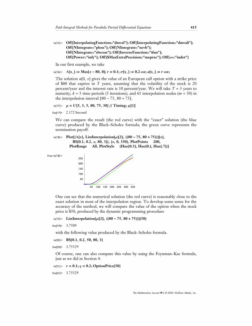
In[16]:= L@x_D := Max@x - 80, 0D; r = 0.1; s@x_D := 0.2 ¥ x; a@x_D := r ¥ x;

The solution u@0, xD gives the value of an European call option with a strike priceof $80 that expires in T years, assuming that the volatility of the stock is 20percent/year and the interest rate is 10 percent/year. We will take T = 3 years tomaturity, k = 5 time periods (5 iterations), and 61 interpolation nodes (m = 30) inthe interpolation interval P80 - 75, 80 + 75T.

In[17]:= m = U@5, 3, 5, 80, 75, 30D êê Timing; mP1TOut[17]= 2.172 Second

We can compare the result (the red curve) with the “exact” solution (the bluecurve) produced by the Black–Scholes formula; the green curve represents thetermination payoff.

In[18]:= Plot@8L@xD, ListInterpolation@mP2T, 8880 - 75, 80 + 75<<D@xD,[email protected], 0.2, x, 80, 3D<, 8x, 0, 350<, PlotPoints Æ 200,

PlotRange Æ All, PlotStyle Æ [email protected], [email protected], [email protected]<DFrom In[18]:=

50 100 150 200 250 300 350

50

100

150

200

250

One can see that the numerical solution (the red curve) is reasonably close to theexact solution in most of the interpolation region. To develop some sense for theaccuracy of the method, we will compare the value of the option when the stockprice is $50, produced by the dynamic programming procedure

In[19]:= ListInterpolation@mP2T, 8880 - 75, 80 + 75<<D@50DOut[19]= 3.7509

with the following value produced by the Black–Scholes formula.

In[20]:= [email protected], 0.2, 50, 80, 3DOut[20]= 3.75529

Of course, one can also compute this value by using the Feynman–Kac formula,just as we did in Section 4.

In[21]:= r = 0.1; V = 0.2; OptionPrice@50DOut[21]= 3.75529

As was pointed out earlier, when the coefficients are linear, y[] gives the exactsolution and one can get away with a single iteration, that is, with a time stepequal to the entire time interval. Essentially this comes down to using theFeynman–Kac formula directly.



As was pointed out earlier, when the coefficients are linear, y[] gives the exactsolution and one can get away with a single iteration, that is, with a time stepequal to the entire time interval. Essentially this comes down to using theFeynman–Kac formula directly.

In[22]:= m = U@1, 3, 1, 80, 75, 30D; ListInterpolation@m, 8880 - 75, 80 + 75<<D@50DOut[22]= 3.75083

The only reason the last two results are different is that U@D applies theFeynman–Kac formula to the interpolated payoff, while OptionPrice@D appliesthe Feynman–Kac formula to the actual payoff. Of course, there is no reason touse the dynamic programming procedure when the coefficients are linear andone deals with a fixed boundary value problem; here we did so only for thepurpose of illustration.

Now we will consider an example in which the coefficients s@D and a@D are notlinear, and therefore the Feynman–Kac formula cannot be used directly, that is,with a single iteration.

In[23]:= s@x_D := 0.3 I1 - 0.9 „-0.02 H40-xL2 M ¥ x; r = 0.1;a@x_D := r ¥ x; L@x_D := Max@x - 40, 0D

With this choice of the coefficients s@D and a@D and the terminal data L@D, thesolution of the PDE in (6.1) will give the price of a call option with a strike priceof $40, but with stochastic volatility for the underlying asset. For the purpose ofillustration, we choose a volatility coefficient that depends on the price of thestock: it decreases to 0.1 when the price of the stock approaches the strike priceof the option and stays constant at 0.2 when the stock price is away from thestrike price.

In[24]:= PlotA s@xDÄÄÄÄÄÄÄÄÄÄÄÄÄÄÄÄ

x, 8x, 0.05, 80<, PlotRange Æ All, PlotPoints Æ 200E

From In[24]:=

20 40 60 800.05

0.15

0.2

0.25

0.3

In[25]:= mk = U @20, 3, 20, 50, 48, 50D êê Timing; mkP1TOut[25]= 14.828 Second

Now we can compare the price of this option with the one produced by theBlack–Scholes formula (the blue line), which ignores the fact that the volatilitydecreases when the stock price approaches the strike price. Just as one wouldexpect, when the stock price is away from the region where the volatilitydecreases, the price of the option looks the same as the price produced under theassumption of constant volatility.

416 Andrew Lyasoff


In[26]:= Plot@[email protected], 0.3, x, 40, 3D, ListInterpolation@mkP2T, 8850 - 48, 50 + 48<<D@xD<,8x, 0, 80<, PlotPoints Æ 400, PlotStyle Æ [email protected], [email protected]<DFrom In[26]:=

20 40 60 80

10

20

30

40

50

When the stock price is $50, the price of this option is

In[27]:= ListInterpolation@mkP2T, 8850 - 48, 50 + 48<<D@50DOut[27]= 20.4144

Notice that we have chosen the interpolation interval P50 - 48, 50 + 48T so thatit is centered around the stock price of interest, namely $50; remember that theaccuracy of the method is the highest at the center of the interpolation interval.Notice also that, while it took much longer to compute, the calculation of theoption price under stochastic volatility did not require any additional work.

Our next example, which is unrelated to finance, will compute the solutionx ö u@0, xD of the equation

∑t u@t, xD + ‰-x2 ∑x,x u@t, xD + Sin@xD ∑x u@t, xD = 0

with boundary condition u@3, xD = [email protected][28]:= s@x_D := "####2 „-

x2ÄÄÄÄÄÄÄÄÄÄ2 ; a@x_D := Sin@xD; L@x_D := Sign@xD; r = 0;

The interpolation interval is P0 - 5, 0 + 5T, the number of interpolation nodes is2 µ 25 + 1 = 51, and the time step is 3ÅÅÅÅÅÅÅ30 = 0.1.

In[29]:= g0 = U@30, 3., 30, 0, 5, 25D êê Timing; g0P1TOut[29]= 10.656 Second

Now we can compare the solution that we just found, that is, the function u@0, ÿ D(pictured as the blue line below) with the terminal data u@3, ÿD (pictured as thered line).

In[30]:= Plot@8L@xD, ListInterpolation@g0P2T, 88-5, 5<<D@xD<,8x, -4.5, 4.5<, PlotStyle Æ 8Hue@0D, [email protected]<, PlotPoints Æ 200DFrom In[30]:=

-4 -2 2 4

-1

-0.5

0.5

1

Sometimes one must use the dynamic programming procedure in a nontrivialway and work with some small time step, even if the coefficients s@D and a@Dhappen to be linear; such a case is an optimal stopping problem, which leads toboundary conditions prescribed along a free boundary. Now we will considerseveral examples that involve stock options in which early exercise is possible (theso-called American options). We only need to change the definition of thefunction U @D; everything else in the procedure will remain the same.



Sometimes one must use the dynamic programming procedure in a nontrivialway and work with some small time step, even if the coefficients s@D and a@Dhappen to be linear; such a case is an optimal stopping problem, which leads toboundary conditions prescribed along a free boundary. Now we will considerseveral examples that involve stock options in which early exercise is possible (theso-called American options). We only need to change the definition of thefunction U@D; everything else in the procedure will remain the same.

In[31]:= U @i_, T_, k_, S_, h_, m_D :=ikjjjjjjjj f @x_D = ListInterpolation@U@i - 1, T , k, S, h, mD, 88S - h, S + h<<D@xD; TableAMaxALAS + j ¥

hÄÄÄÄÄÄÄÄm

E, „-r¥TÄÄÄÄÄÄÄk

ÄÄÄÄÄÄÄÄÄÄÄÄÄÄÄÄÄÄÄÄÄè!!!!!!!2 p

¥ NIntegrateA f AyA TÄÄÄÄÄÄÄÄk

, S + j ¥h

ÄÄÄÄÄÄÄÄm

, yEE „- y2ÄÄÄÄÄÄÄÄÄÄÄÄÄÄÄ2 ,

8 y, -7, 7<, MaxRecursion Æ 20EE, 8 j, -m, m<Ey{zzzzzzzzUnder the Black–Scholes assumption for the price process, American call optionsare the same as European call options because early exercise of such options isnever optimal. Thus, in our first example we consider an American put optionwith a strike price of $40.

In[32]:= L@x_D := Max@40 - x, 0DFirst, we will compute the price of the option under the assumption that—just asin the Black–Scholes model—the stock price follows a geometric Brownianmotion process (of course, the Black–Scholes formula cannot be used in this caseas is, for it is only valid for European options).

In[33]:= r = 0.1; s@x_D := 0.2 ¥ x; a@x_D := r ¥ x;

We will interpolate the solution in the interval P40 - 38, 40 + 38T ª P2, 78T with41 interpolation nodes and use 20 iterations, which amounts to a time step of0.15.

In[34]:= m = U@20, 3, 20, 40, 38, 20D êê Timing; mP1TOut[34]= 6.438 Second

Now we can plot the solution (the red curve below) together with the termina-tion payoff function (the blue curve).

In[35]:= Plot@8L@xD, ListInterpolation@mP2T, 8840 - 38, 40 + 38<<D@xD<,8x, 0, 80<, PlotPoints Æ 200, PlotStyle Æ [email protected], [email protected]<DFrom In[35]:=

20 40 60 80

10

20

30

40

To those familiar with the basics of American options, it should be clear fromthis graph that the approximation that we just produced is not very accurate inthe last 1/4 of the interpolation interval (it is well known that the actual stockprice decreases to 0 monotonically). This is caused by the fact that, when theprocess Xt , t r 0, starts from a point that is close to the end of the interpolationinterval, a sizeable part of the distribution of Xt might be spread in the regionwhere the procedure is forced to use extrapolation. As a result, depending onhow far inside the extrapolation region the essential part of the distribution of Xtgoes, the error from the extrapolation can be significant. In this particularexample, one possible remedy would be to set u@T - Hi - 1L T -tÅÅÅÅÅÅÅÅÅÅÅk , xD to 0 for allsufficiently large values of x, regardless of the value produced by the interpola-tion (or the extrapolation) procedure. This is a common problem in essentiallyall numerical methods for PDEs, and the common way around it is to work witha grid in the state-space which covers a considerably larger region than the onein which an accurate representation of the solution is being sought. It is to benoted, however, that, as k Ø ¶, that is, as the time step converges to 0, thesolution produced after k iterations will converge to the actual solution in theentire interpolation interval. This is because when the process Xt , t r 0, startsfrom one of the end-points of that interval, for a very small value of t, the distribu-tion of Xt will be concentrated mostly around the end-point where the extrapola-tion procedure is still reasonably accurate. Thus, by using the method developedhere, one can construct an arbitrarily accurate representation of the solution inthe entire interpolation interval by simply choosing a sufficiently large number ofinterpolation nodes and a sufficiently small time step. In general, this is not truefor the finite difference method. In order to illustrate this phenomenon, we willnow repeat the above calculation with a time step, which is three times as small(accordingly, the calculation will run about three times longer).

418 Andrew Lyasoff


To those familiar with the basics of American options, it should be clear fromthis graph that the approximation that we just produced is not very accurate inthe last 1/4 of the interpolation interval (it is well known that the actual stockprice decreases to 0 monotonically). This is caused by the fact that, when theprocess Xt , t r 0, starts from a point that is close to the end of the interpolationinterval, a sizeable part of the distribution of Xt might be spread in the regionwhere the procedure is forced to use extrapolation. As a result, depending onhow far inside the extrapolation region the essential part of the distribution of Xtgoes, the error from the extrapolation can be significant. In this particularexample, one possible remedy would be to set u@T - Hi - 1L T -tÅÅÅÅÅÅÅÅÅÅÅk , xD to 0 for allsufficiently large values of x, regardless of the value produced by the interpola-tion (or the extrapolation) procedure. This is a common problem in essentiallyall numerical methods for PDEs, and the common way around it is to work witha grid in the state-space which covers a considerably larger region than the onein which an accurate representation of the solution is being sought. It is to benoted, however, that, as k Ø ¶, that is, as the time step converges to 0, thesolution produced after k iterations will converge to the actual solution in theentire interpolation interval. This is because when the process Xt , t r 0, startsfrom one of the end-points of that interval, for a very small value of t, the distribu-tion of Xt will be concentrated mostly around the end-point where the extrapola-tion procedure is still reasonably accurate. Thus, by using the method developedhere, one can construct an arbitrarily accurate representation of the solution inthe entire interpolation interval by simply choosing a sufficiently large number ofinterpolation nodes and a sufficiently small time step. In general, this is not truefor the finite difference method. In order to illustrate this phenomenon, we willnow repeat the above calculation with a time step, which is three times as small(accordingly, the calculation will run about three times longer).

In[36]:= mm = U@60, 3, 60, 40, 38, 20D êê Timing; mmP1TOut[36]= 14.89 Second

In[37]:= Plot@8L@xD, ListInterpolation@mmP2T, 8840 - 38, 40 + 38<<D@xD<,8x, 0, 80<, PlotPoints Æ 200, PlotStyle Æ [email protected], [email protected]<DFrom In[37]:=

20 40 60 80

10

20

30

40

Let us remember that here we are also solving an optimal stopping problem,whose solution is given by the point, which separates the “exercise” region, thatis, the region where the price of the option coincides with the terminationpayoff, from the “hold” region, where the price of the option is larger than thetermination payoff.



In[38]:= FindRoot@ListInterpolation@mmP2T, 8840 - 38, 40 + 38<<D@xD ä Max@40 - x, 0D,8x, 38, 40<DOut[38]= 8x Ø 34.3<

It is interesting that the solution, which was produced earlier and about threetimes faster by using a three times larger time step, gives the same result.

In[39]:= FindRoot@ListInterpolation@mP2T, 8840 - 38, 40 + 38<<D@xD ä Max@40 - x, 0D,8x, 38, 40<DOut[39]= 8x Ø 34.3<

This illustrates perfectly the point that we made earlier: the result produced withthe larger time step was already reasonably accurate in the middle of the interpola-tion interval.

Now we will compute the price of the same put option, but under the assump-tion that the stock price exhibits stochastic volatility of the type we introducedearlier in conjunction with European-type options.

In[40]:= s@x_D := 0.2 ¥ I1 - 0.5 „-0.01¥H40-xL2 M ¥ x;r = 0.1; a@x_D := r ¥ x; L@x_D := Max@40 - x, 0D

In[41]:= mx = U@60, 3, 60, 40, 38, 30D êê Timing; mxP1TOut[41]= 26.547 Second

Now we can compare the last result (the blue curve below) with the one that wasproduced in the case of constant volatility (the red curve).

In[42]:= Plot@8L@xD, ListInterpolation@mmP2T, 8840 - 38, 40 + 38<<D@xD,ListInterpolation@mxP2T, 8840 - 38, 40 + 38<<D@xD<, 8x, 30, 70<,

PlotPoints Æ 200, PlotStyle Æ [email protected], [email protected], [email protected]<DFrom In[42]:=

40 50 60 70

2

4

6

8

10

We can see that, just as one would expect, the price of this option differs fromthe one produced under the constant volatility assumption only in the regionwhere the volatility decreases. Also, the decrease of the volatility near the exer-cise price actually decreases the range of stock prices for which immediateexercise is optimal, as the following computation shows.

In[43]:= FindRoot@ListInterpolation@mxP2T, 8840 - 38, 40 + 38<<D@xD ä Max@40 - x, 0D,8x, 23, 30<DOut[43]= 8x Ø 30.<

420 Andrew Lyasoff


‡ 7. Concluding RemarksAlthough the examples presented in Section 6 were borrowed mostly from therealm of computational finance, it is important to realize that neither the generalmethod developed in Sections 3 and 5, nor the Mathematica code used inSection 6 takes advantage of the special nature of the problems associated withfinancial applications in any way. The same method—and, indeed, the samecomputer code—can produce an approximate solution to a rather general one-di-mensional parabolic PDE with boundary conditions imposed on some free orfixed boundary. Furthermore, this method does not require any manipulationwhatsoever of the PDE.

As is well known, the “no free lunch” principle reigns in the world of computing,too, and the simplicity, the generality, and the precision with which we were ableto solve some classical option valuation problems in the previous section did notcome easily by any means. In terms of this metaphor, not only was the lunch notfree, but it was, in fact, a rather expensive one. Indeed, an efficient integrationprocedure was absolutely crucial for the implementation of the method inSection 6. As explained in The Mathematica Book (see [8] p. 1071) the functionIntegrate[ ] “uses about 500 pages of Mathematica code and 600 pages of C code.”The role played by the function ListInterpolation[ ] was just as crucial. Indeed, itallowed us to work on an exceptionally coarse grid in the state-space and then“restore” the values at all remaining points by a fairly sophisticated interpolationprocedure. More importantly, we were able to feed NIntegrate[ ] with the objectproduced by ListInterpolation[ ]. There are intrinsic obstacles to such “shortcuts”in essentially all modifications of the finite difference method.

‡ AcknowledgmentThis work is dedicated to D. W. Stroock and S. R. S. Varadhan. All numericalprocedures used here are a mere transcript of their insights.

‡ References[1] F. Black and M. Scholes, “The Pricing of Options and Corporate Liabilities,” Journal of

Political Economy, 81, 1973 pp. 637–659.

[2] D. W. Stroock and S. R. S. Varadhan, “Multidimensional Diffusion Processes,” Grundle-hren der Mathematischen Wissenschaften [Fundamental Principles of MathematicalSciences], 233, New York, Berlin: Springer-Verlag, 1979.

[3] D. W. Stroock, “Lectures on Stochastic Analysis: Diffusion Theory,” London Mathemati-cal Society Student Texts, 6, 1987, Oxford: Cambridge University Press.

[4] D. W. Stroock, Probability Theory, an Analytic View, Oxford: Cambridge UniversityPress, 1993.

[5] A. Lyasoff, “Three Page Primer in Financial Calculus.” (2000) Boston: Boston University.www.bu.edu/mathfn/people/primer1.pdf.



[6] P. E. Kloeden and E. Platen, Numerical Solutions of Stochastic Differential Equations,New York: Springer-Verlag, 1997.

[7] D. Stroock and S. Taniguchi, “Diffusions as Integral Curves, or Stratonovich without Itô,”in Progress in Probability #34, ed. by M. Freidlin, Birkhäuser, 1994, pp. 331–369.

[8] S. Wolfram, The Mathematica Book, 5th ed. Champaign, Oxford: Wolfram Media/Cambridge University Press, 1999.

About the AuthorAndrew Lyasoff is associate professor and director of the M.A. degree program inMathematical Finance at Boston University. His research interests are mostly in thearea of Stochastic Calculus and Mathematical Finance. Over the last few years hehas been using Mathematica extensively to develop new numerical methods for PDEsand new instructional tools for graduate courses in Operations Research and Mathe-matical Finance. In addition, he is developing new theoretical models that reflectlong-range dependencies in market data.

Andrew LyasoffBoston UniversityDepartment of Mathematics and StatisticsBoston, [email protected]

422 Andrew Lyasoff


path integral methods for parabolic partial differential ... · pdf filethe mathematica®...

Documents