Path Planning vs. Obstacle Avoidance

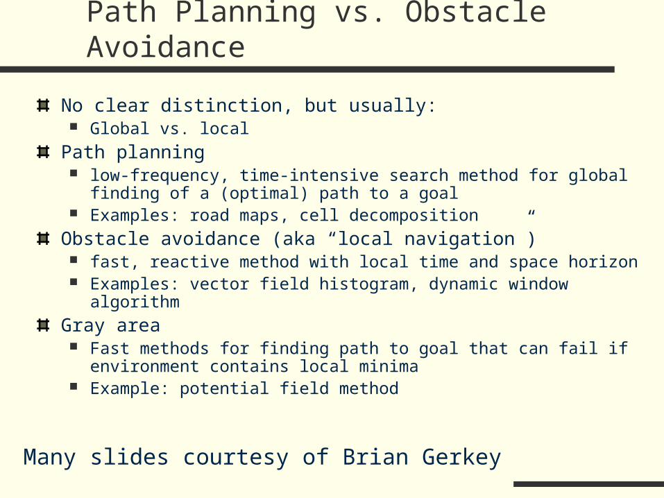
No clear distinction, but usually: Global vs. local

Path planning low-frequency, time-intensive search method for global finding of a (optimal) path

to a goal Examples: road maps, cell decomposition

Obstacle avoidance (aka “local navigation”) fast, reactive method with local time and space horizon Examples: vector field histogram, dynamic window algorithm

Gray area Fast methods for finding path to goal that can fail if environment contains local

minima Example: potential field method

Many slides courtesy of Brian Gerkey

Local minima

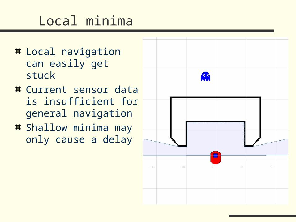
Local navigation can easily get stuck

Current sensor data is insufficient for general navigation

Shallow minima may only cause a delay

Deep minima

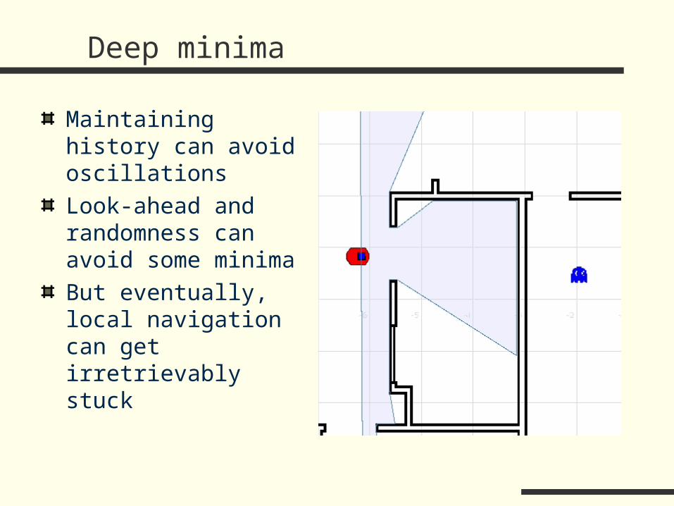
Maintaining history can avoid oscillations

Look-ahead and randomness can avoid some minima

But eventually, local navigation can get irretrievably stuck

Our goal

Given: map robot pose goal pose

Compute: a feasible (preferably

efficient) path to the goal

Also, execute the path may require replanning

Configuration space

workspace (W): The ambient environment in which the robot operates Usually R2 or R3

configuration (q): Complete specification of the position of all points in the robot’s body Set of points in robot’s body is given by R(q)

configuration space, or C-space (Q): Space of all possible configurations C-space dimensionality = # degrees of freedom

Example 1: two-link arm

Two angles fully specify the configuration 2-dimensional configuration

space Q = (1, 2)

Is the position of the end effector a valid configuration specification? Q ?= (X, Y)

Example 2: Sony AIBO

4 legs, 3 dof each 2 in the shoulder 1 in the knee

1 head, 3 dof

15 dof => 15-d C-space Q = (l1,l2,l3,l4,h)

+ 6 DOF real-world pose

Example 3: planar mobile robot

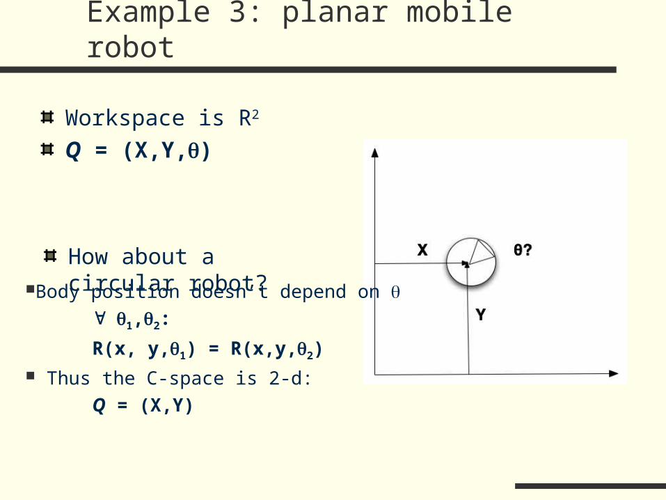
Workspace is R2

Q = (X,Y,)

How about a circular robot?Body position doesn’t depend on

1,2:

R(x, y,1) = R(x,y,2) Thus the C-space is 2-d:

Q = (X,Y)

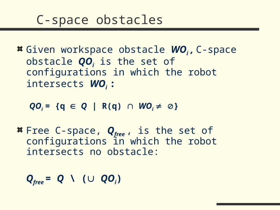
C-space obstacles

Given workspace obstacle WOi , C-space obstacle QOi is the set of configurations in which the robot intersects WOi :

QOi = {q Q | R(q) WOi }

Free C-space, Qfree , is the set of configurations in which the robot intersects no obstacle:

Qfree = Q \ ( QOi)

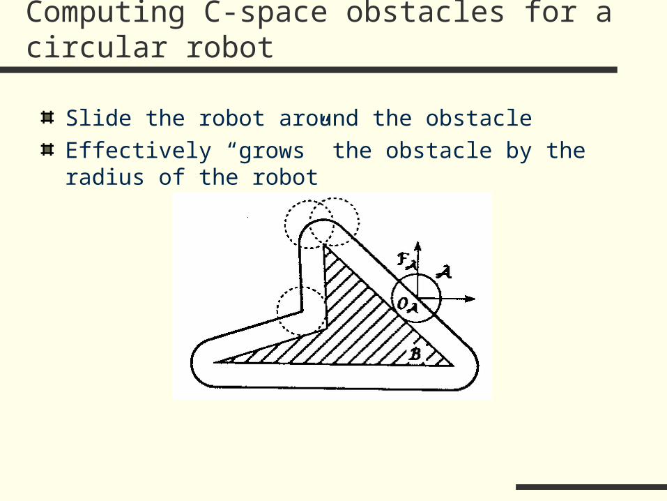
Computing C-space obstacles for a circular robot

Slide the robot around the obstacle

Effectively “grows” the obstacle by the radius of the robot

C-space, radius=1.0m

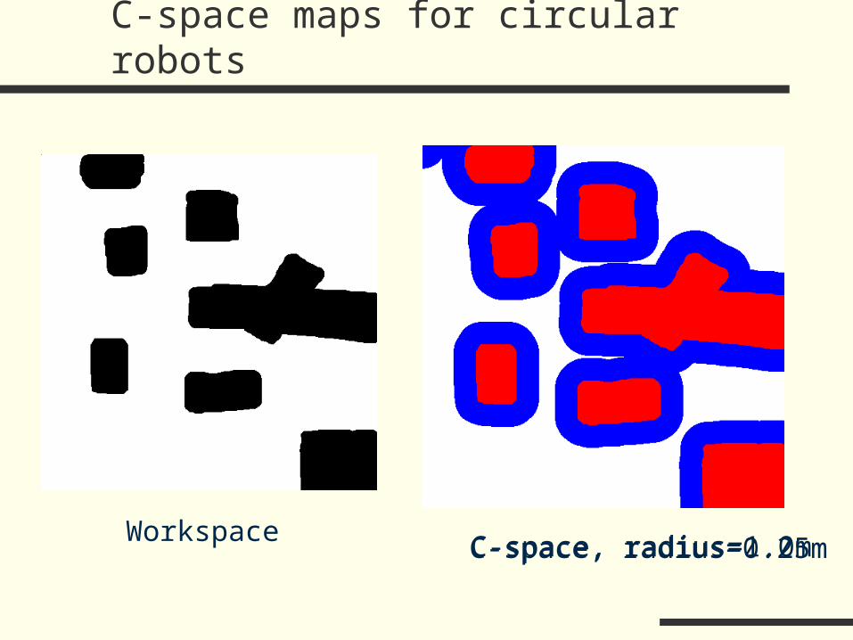
C-space maps for circular robots

WorkspaceC-space, radius=0.25m

10/31/06 CS225B Brian Gerkey

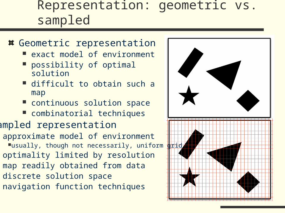
Representation: geometric vs. sampled

Geometric representation exact model of environment possibility of optimal solution difficult to obtain such a map continuous solution space combinatorial techniques

Sampled representation approximate model of environment

usually, though not necessarily, uniform grid optimality limited by resolution map readily obtained from data discrete solution space navigation function techniques

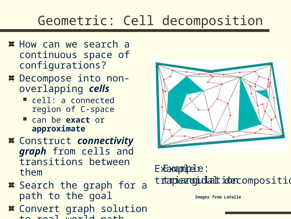
Geometric: Cell decomposition

How can we search a continuous space of configurations?Decompose into non-overlapping cells cell: a connected region of C-space can be exact or approximate

Construct connectivity graph from cells and transitions between themSearch the graph for a path to the goalConvert graph solution to real-world path

Example:trapezoidal decompositionExample:triangulation

Images from LaValle

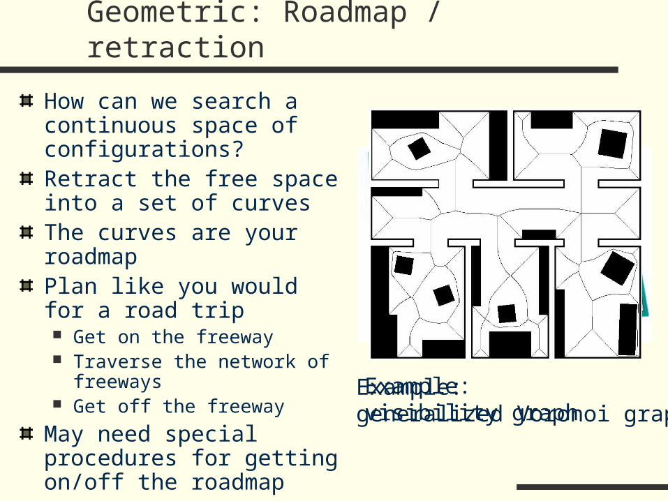
Geometric: Roadmap / retraction

How can we search a continuous space of configurations?Retract the free space into a set of curvesThe curves are your roadmapPlan like you would for a road trip Get on the freeway Traverse the network of freeways Get off the freeway

May need special procedures for getting on/off the roadmap Example:

visibility graphExample:generalized Voronoi graph

10/31/06 CS225B Brian Gerkey

Sampled: potential / navigation functions

For each sampled state, estimate the cost to goal similar to a policy in machine learning

Grid maps: for each cell, compute the cost (number of cells, distance, etc.) to the goalpotential functions are local

Images from LaValle

navigation functions are global

wavefront planner

Given grid map M, robot position p, goal position g

From M, create C-space map MQ

Run brushfire algorithm on MQ: Label grid cell g with a “0” Label free cells adjacent to g with a “1” Label free cells adjacent to those cells with a “2” Repeat until you reach p

Labels encode length of shortest (Manhattan distance) obstacle-free path from each cell to gStarting from p, follow the gradient of labelsComplete

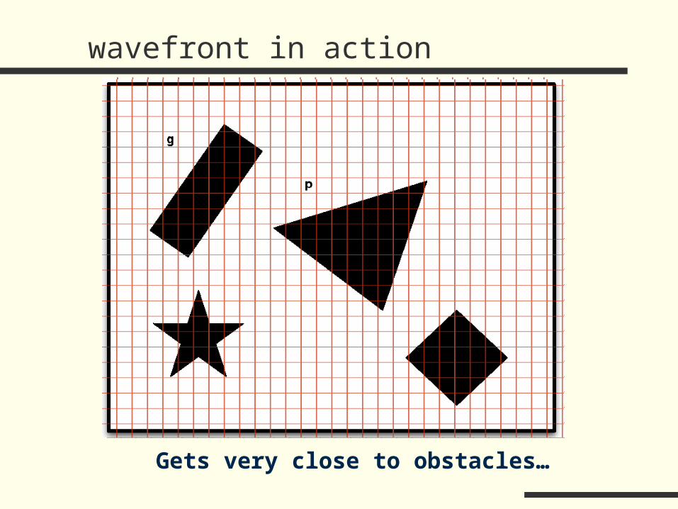
wavefront in action

Gets very close to obstacles…

Inefficient paths

Naïve single-neighbor cost update gives Manhattan distance (maybe with diagonal transitions) The gradient unnecessarily tracks the grid

Graphic fromFerguson and Stentz , Field-D*

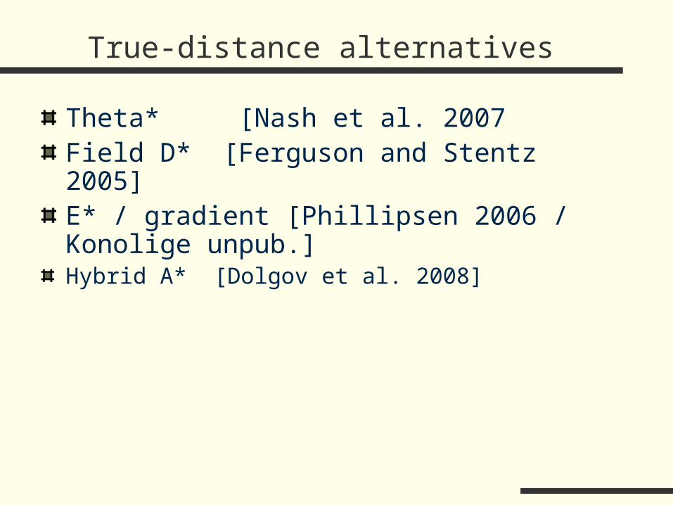
True-distance alternatives

Theta* [Nash et al. 2007Field D* [Ferguson and Stentz 2005]E* / gradient [Phillipsen 2006 / Konolige unpub.]Hybrid A* [Dolgov et al. 2008]

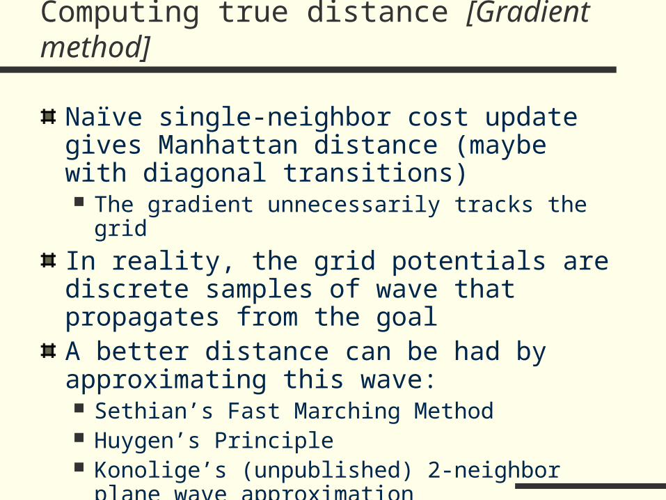
Computing true distance [Gradient method]

Naïve single-neighbor cost update gives Manhattan distance (maybe with diagonal transitions) The gradient unnecessarily tracks the grid

In reality, the grid potentials are discrete samples of wave that propagates from the goalA better distance can be had by approximating this wave: Sethian’s Fast Marching Method Huygen’s Principle Konolige’s (unpublished) 2-neighbor plane wave

approximation

Interpolating a potential function

a

bc?

c = fn(a,b) Planar wave approximation

F

a << b => c = a + F

F is the intrinsic cost of motion

isopotentials

Interpolating a potential function

a

bc?

c = fn(a,b) Planar wave approximation

F

a = b => c = a + (1/sqrt(2))*F

F is the intrinsic cost of motion

isopotentia

ls

Interpolating a potential function

a

bc?

c = fn(a,b) Planar wave approximation

F

a < b => c = ???

F is the intrinsic cost of motion

isopotentials

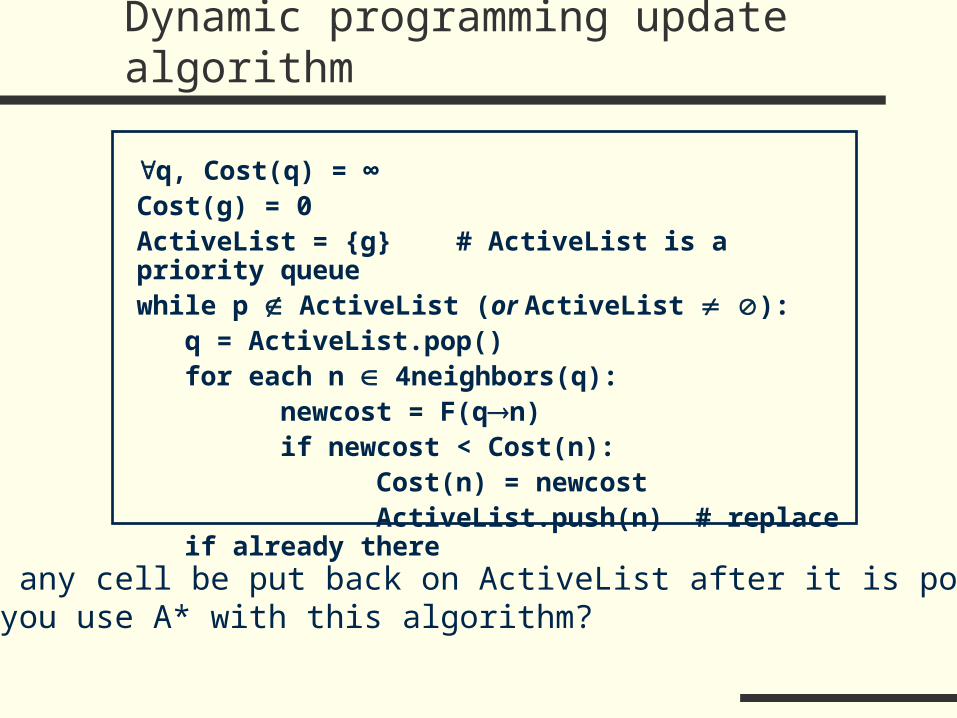
Dynamic programming update algorithm

q, Cost(q) = ∞Cost(g) = 0ActiveList = {g} # ActiveList is a priority queuewhile p ActiveList (or ActiveList ):

q = ActiveList.pop()for each n 4neighbors(q):

newcost = F(qn)if newcost < Cost(n):

Cost(n) = newcostActiveList.push(n) # replace if already

there

Will any cell be put back on ActiveList after it is popped?Can you use A* with this algorithm?

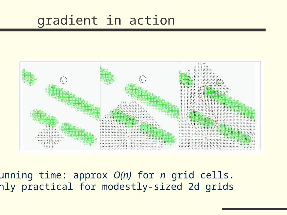
gradient in action

Running time: approx O(n) for n grid cells.Only practical for modestly-sized 2d grids

Obstacle costs

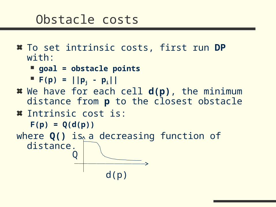
To set intrinsic costs, first run DP with: goal = obstacle points F(p) = ||pj - pi||

We have for each cell d(p), the minimum distance from p to the closest obstacleIntrinsic cost is:F(p) = Q(d(p))

where Q() is a decreasing function of distance.

d(p)

Q

Finding the gradient

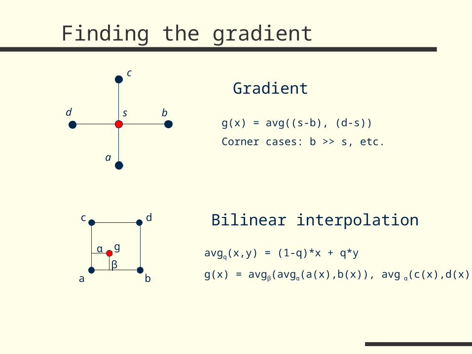
Bilinear interpolation

a b

c d

gα

βavgq(x,y) = (1-q)*x + q*y

g(x) = avgβ(avgα(a(x),b(x)), avg α(c(x),d(x)))

a

bsd

c

Gradient

g(x) = avg((s-b), (d-s))

Corner cases: b >> s, etc.

Gradient in LAGR Test 26A

Gradient with A*

Practical concerns

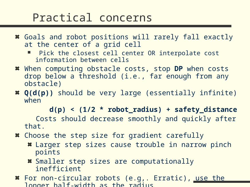
Goals and robot positions will rarely fall exactly at the center of a grid cell Pick the closest cell center OR interpolate cost information between cells

When computing obstacle costs, stop DP when costs drop below a threshold (i.e., far enough from any obstacle)Q(d(p)) should be very large (essentially infinite) when

d(p) < (1/2 * robot_radius) + safety_distance Costs should decrease smoothly and quickly after that.

Choose the step size for gradient carefullyLarger step sizes cause trouble in narrow pinch pointsSmaller step sizes are computationally inefficient

For non-circular robots (e.g,. Erratic), use the longer half-width as the radius No longer complete, but usually works

10/31/06 CS225B Brian Gerkey

Dealing with local obstacles

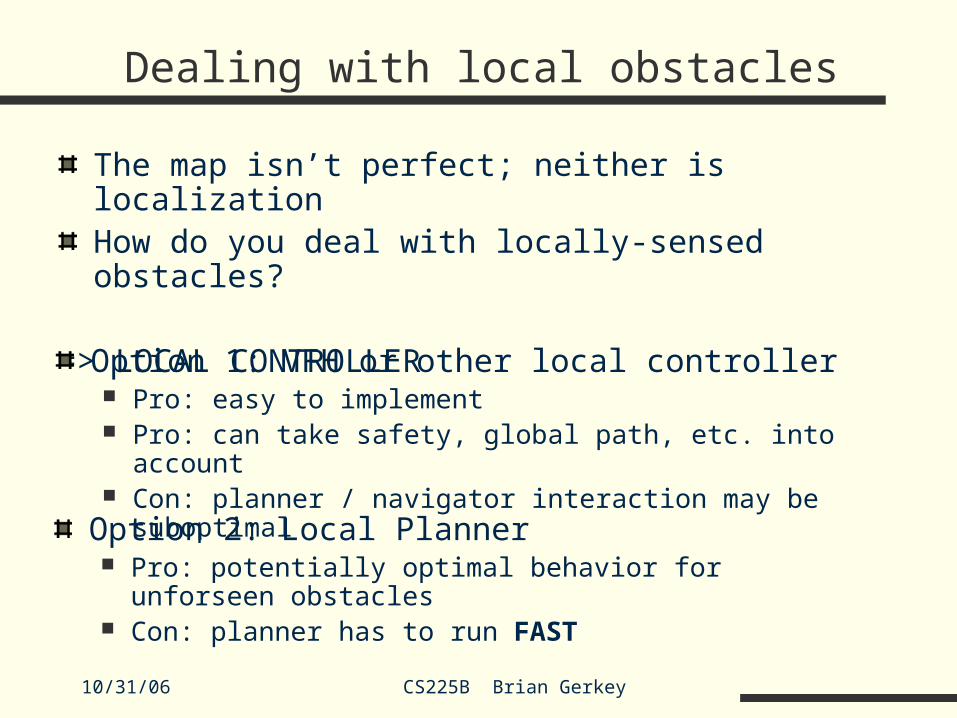
The map isn’t perfect; neither is localizationHow do you deal with locally-sensed obstacles?

=> LOCAL CONTROLLER

Option 1: VFH or other local controller Pro: easy to implement Pro: can take safety, global path, etc. into account Con: planner / navigator interaction may be suboptimal

Option 2: Local Planner Pro: potentially optimal behavior for unforseen obstacles Con: planner has to run FAST

10/31/06 CS225B Brian Gerkey

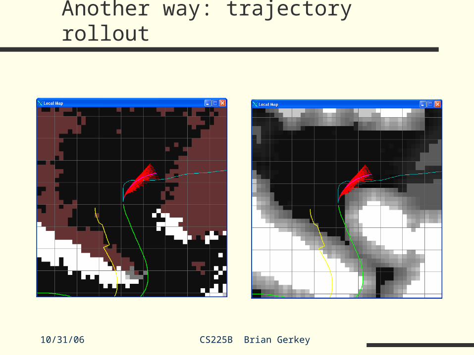
Another way: trajectory rollout

10/31/06 CS225B Brian Gerkey

Gradient + trajectory rollout in exploration: LAGR

Average speed > 1m/s

LAGR-Eucalyptus run

LAGR-Eucalyptus run - montage

LAGR-Eucalyptus run - map

10/31/06 CS225B Brian Gerkey

Local Planner

Pick some small area to do local planning Look ahead on global plan for the local goal point Add in local obstacles from sensors

Things to look out for: How do you track the local path? When do you replan the global plan?

10/31/06 CS225B Brian Gerkey

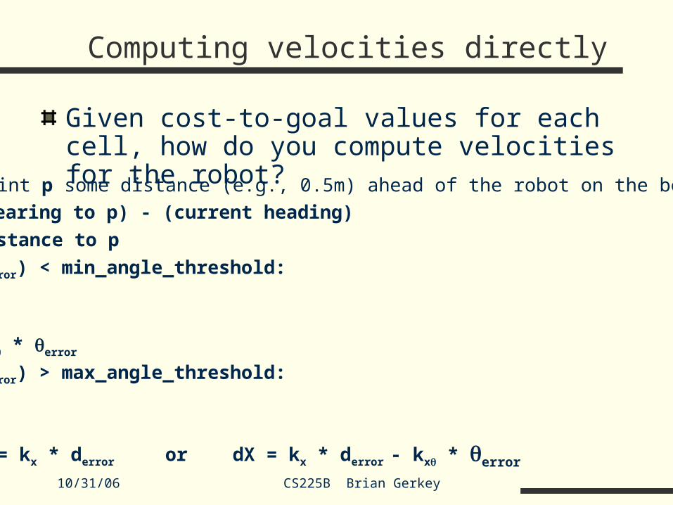
Computing velocities directly

Given cost-to-goal values for each cell, how do you compute velocities for the robot?

Pick a point p some distance (e.g., 0.5m) ahead of the robot on the best path

error = (bearing to p) - (current heading)

derror = distance to p

if abs(error) < min_angle_threshold:d = 0

else:

d = k * error

if abs(error) > max_angle_threshold:dX = 0

else:

dX = kx * derror or dX = kx * derror - kx * error