paths, smoothing, least squares fit cs 551/651 spring 2002
TRANSCRIPT
Paths, Smoothing, Least Squares Fit
CS 551/651
Spring 2002

Following a Path
• How do we compute an object’s first-person view as it follows a path?– Situate a local coordinate system about the
object and orient the system• Positive z-axis points frontward
– Frontward is first derivative, P’(s)
• Positive y-axis points upward– Upward is cross product of z-axis and P’’(s)
• Positive x-axis points left– Cross product of z- and y-axes

Newton-Raphson
• No guarantees that it will find the roots of an equation
• Or that it will be efficient CaughtHere

Cross Product Right Hand Rule
• See: http://www.phy.syr.edu/courses/video/RightHandRule/index2.html
• Orient your right hand such that your palm is at the beginning of A and your fingers point in the direction of A
• Twist your hand about the A-axissuch that B extends perpendicularly from your palm
• As you curl your fingers to make a fist, your thumb will point in the direction of the cross product

Frenet Frame
• The local coordinate system
• If curve has no curvature, technique fails– Use Frenet Frame from before straight
section starts (and interpolate rotation about z-axis if necessary)
• Use dot product of y-axis before and after straight section to determine interpolation amount

Frenet Frame
• Discontinuity in the curvature causes jump in local coordinate system
• Can be jumpy if curve is not very smooth
• Doesn’t reflect desirable camera effects like banking into a corner
• A curve that moves downward in 3-space will cause Frenet frame to orient upside-down

Alternative Orientation Methods
• Define a natural notion of ‘UP’, y-axis– The opposite direction of gravity
• Define a focal point, z-axis– z-axis = focal_point – cur_pos– x-axis = z-axis x UP– y-axis = z-axis x x-axis
• Passing close to focal point causes extreme changes
• How do you automatically update focal point?
Lookahead
• If cur_pos = p(s), the focal point = p(s+s)– Note, should be arc length parameterization
to prevent wandering camera
• What about the end of curve (where s+s is undefined)?– Extrapolate curve in the direction of its
tangent

Smoothing Data
• Frequently we use a series of points to represent paths
• We turn points into piecewise Bezier curve
• But may be overkill
• Alternatives

Smoothing Data
• Average a point with its neighbors
– But this causes flattening of curves
• Fit cubic curve to subsets of points– Curve is inherently smooth– Sample curve at midpoint for new point
11
11
4
1
2
1
4
1
22
iii
iii
i PPP
PPP
P

Cubic Curves
• P(u) = au3 + bu2 + cu + d
• For a point, Pi, build curve from its four neighbors– Pi-2, Pi-1, Pi+1, Pi+2
– Evaluate the cubic at its midpoint (u = ½)
– Average cubic midpoint and Pi

Evaluating the Cubic
• Pi-2 = P(0) = d
• Pi-1 = P(1/4) = a 1/64 + b 1/16 + c1/4 + d
• Pi+1 = P(3/4) = a 27/64 + b 9/16 + c¾ + d
• Pi+2 = P(1) = a + b + c + d
• 4 equations and 4 unknowns… solve

Evaluating Cubic
• What about endpoints?• Pi+1 and Pi+2 don’t exist
– P’0 = P3 + 3 (P1 – P2)
• Second in from beginning or end?– Build a quadratic (parabola)– P(u) = au2 + bu + c– Solve for a, b, and c using P0, P2, P3
– P1 is averaged with P(1/3)

Overconstrained Cubics
• Earlier, we solved for cubic coefficients using Gaussian Elimination / Linear Programming
• We solved for x such that Ax = b
• A was square and invertable
3
2
1
0
23
23
11114
3
4
3
4
3
4
3
14
1
4
1
4
11000
P
P
P
P
d
c
b
a
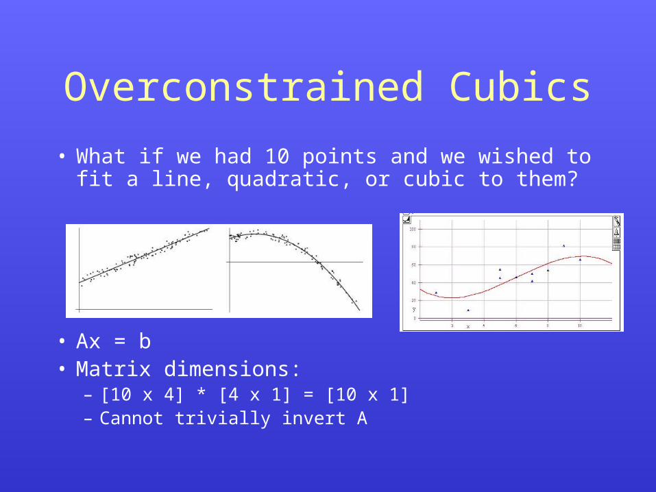
Overconstrained Cubics
• What if we had 10 points and we wished to fit a line, quadratic, or cubic to them?
• Ax = b• Matrix dimensions:
– [10 x 4] * [4 x 1] = [10 x 1]– Cannot trivially invert A

Least Squares Fit
• Select a cubic curve (the x-vector in our example) that minimizes the standard deviation of the distances between the points and the cubic curve:
10
1
2)(i
ii ufy

Least Squares Fit
• E is the error function:
• f(u) is a function of (a, b, c, d) and u– It is the parametric cubic curve
• We want to minimize E
• Wherever E is minimized:
10
1
223
10
1
2)(
iiiiii
iii
dxcxbxaxy
xfyE
0
d
E
c
E
b
E
a
E

Least Squares Fit
• Compute the partial derivative of E w.r.t. a, b, c, and d
• Set each partial derivative equal to 0• We now have four equations and four
unknowns• Solve…• This method is slow and there are better
least squares solution methods

Linear Least Squares
• We just talked about linear least squares– The cubic equation is nonlinear because x is
raised to powers greater than 1• ax3 + bx2 + cx + d
– But fitting a cubic to a set of data is linear curve fitting
• Parameters (a, b, c, d) enter into the formula as simple multipliers of terms that are added together

An example
• Fit a line to data:– The vertical deviation of the ith piece of data
(xi, yi) is:
• di = yi – y = yi – (mxi + b)
• Where m and b are the unknown parameters
– By minimizing square of deviations• d2
i = (yi – y)2 = (yi – (mxi + b))2

An example
• Minimize sum of di and set partials to 0
M
xmyb
xmMby
mxby
mxbyb
D
mxbyD
M
ii
M
ii
M
ii
M
ii
M
ii
M
i
M
ii
M
iii
M
iii
11
11
111
1
1
2
0
0
0)(2
)(
M
ii
M
i
M
iiii
M
i
M
ii
M
iiii
M
iiii
x
xbyxm
xmxbyx
xmxbym
D
1
2
1 1
1 1
2
1
1
0
0)(2
m=
b=

Computer Tools
• Write your own function• Mathematica
– Fit [data, {1, x}, x]
• Excel– Linest (y-array, x-array, count, statistics)
• See http://www.orst.edu/instruct/ch490/lessons/lesson9.htm
for more info

Robustness of Least Squares
• Effective, complete, and appropriate for many problems in science/engineering
• Estimates of unknowns are optimal• Efficient use of data• Not good for extrapolation past
endpoints• Sensitive to presence of outliers
– Model validation is useful
Convolution Kernels
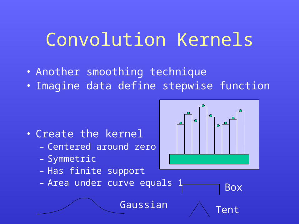
• Another smoothing technique• Imagine data define stepwise function
• Create the kernel– Centered around zero– Symmetric– Has finite support– Area under curve equals 1 Box
Gaussian Tent

Convolution Kernels
• Compute new (averaged) points by convolving kernel with data
• Slide kernel over all points• Watch for overlap at beginning and end
New value for P1 is:
2
0
Overlap) of (AreaP
P
P
Determining a Path on Surface
• Consider a polygonal terrain map
• Assume you have the (x,y,z) coordinates of two endpoints
• What are the values of intermediate points on the line?

Path Determination
• Construct a plane that passes through the two points and is (roughly) perpendicular to the ground plane– How do we compute the perpendicular?– How doe we compute the plane?
• Intersect plane with the terrain polys– How?

Path Determination
• If the terrain is modeled as a parametric surface: f(u, v) = z
• Linearly interpolate between (u1, v1) and (u2, v2) and solve for f(uinterp, vinterp)

Path Determination
• What if ground is constructed from many triangles and we wish to only walk along the edges?– Start from the first point– And then what?
• Consider all coincident edges
• Project each edge to straight line on path. How?
• Dot product (remember to normalize)

Path Determination
• Edge with smallest angle is selected
• Keep applying until destination is reached
• Guaranteed to reach destination?

Downhill Paths
• To go downhill– Cross product of surface normal and ‘up’
gives you a surface tangent vector (perpendicular to down)
– Cross product of surface tangent and normal vector defines downhill vector

Reminder
• Read papers and write questions for Tuesday
• Assignment due Thursday at 9:00 a.m.
• Warping and morphing are next