Pattern Recognition Letters 42 (2014) 11–24

Contents lists available at ScienceDirect

Pattern Recognition Letters

journal homepage: www.elsevier .com/locate /patrec

A review of unsupervised feature learning and deep learningfor time-series modeling q

http://dx.doi.org/10.1016/j.patrec.2014.01.0080167-8655/� 2014 Elsevier B.V. All rights reserved.

q This paper has been recommended for acceptance by A. Petrosino.⇑ Corresponding author. Tel.: +46 19303749.

E-mail addresses: martin.langkvist@oru.se (M. Längkvist), lars.karlsson@oru.se(L. Karlsson), amy.loutfi@oru.se (A. Loutfi).

Martin Längkvist ⇑, Lars Karlsson, Amy LoutfiApplied Autonomous Sensor Systems, School of Science and Technology, Örebro University, SE-701 82 Örebro, Sweden

a r t i c l e i n f o a b s t r a c t

Article history:Received 16 July 2013Available online 28 January 2014

Keywords:Time-seriesUnsupervised feature learningDeep learning

This paper gives a review of the recent developments in deep learning and unsupervised feature learningfor time-series problems. While these techniques have shown promise for modeling static data, such ascomputer vision, applying them to time-series data is gaining increasing attention. This paper overviewsthe particular challenges present in time-series data and provides a review of the works that have eitherapplied time-series data to unsupervised feature learning algorithms or alternatively have contributed tomodifications of feature learning algorithms to take into account the challenges present in time-seriesdata.

� 2014 Elsevier B.V. All rights reserved.

1. Introduction and background

Time is a natural element that is always present when the hu-man brain is learning tasks like language, vision and motion. Mostreal-world data has a temporal component, whether it is measure-ments of natural processes (weather, sound waves) or man-made(stock market, robotics). Analysis of time-series data has beenthe subject of active research for decades [66,26] and is consideredby Yang and Wu [131] as one of the top 10 challenging problems indata mining due to its unique properties. Traditional approachesfor modeling sequential data include the estimation of parametersfrom an assumed time-series model, such as autoregressive models[83] and Linear Dynamical Systems (LDS) [82], and the popularHidden Markov Model (HMM) [103]. The estimated parameterscan then be used as features in a classifier to perform classification.However, more complex, high-dimensional, and noisy real-worldtime-series data cannot be described with analytical equationswith parameters to solve since the dynamics are either too com-plex or unknown [119] and traditional shallow methods, whichcontain only a small number of non-linear operations, do not havethe capacity to accurately model such complex data.

In order to better model complex real-world data, one approachis to develop robust features that capture the relevant information.However, developing domain-specific features for each task isexpensive, time-consuming, and requires expertise of the data.

The alternative is to use unsupervised feature learning [8,5,29] inorder to learn a layer of feature representations from unlabeleddata. This has the advantage that the unlabeled data, which is plen-tiful and easy to obtain, is utilized and that the features are learnedfrom the data instead of being hand-crafted. Another benefit is thatthese layers of feature representations can be stacked to createdeep networks, which are more capable of modeling complexstructures in the data. Deep networks have been used to achievestate-of-the-art results on a number of benchmark data sets andfor solving difficult AI tasks. However, much focus in the featurelearning community has been on developing models for static dataand not so much on time-series data.

In this paper we review the variety of feature learning algo-rithms that has been developed to explicitly capture temporal rela-tionships as well as the various time-series problems that theyhave been used on. The properties of time-series data will be dis-cussed in Section 2 followed by an introduction to unsupervisedfeature learning and deep learning in Section 3. An overview ofsome common time-series problems and previous work using deeplearning is given in Section 4. Finally, conclusions are given inSection 5.

2. Properties of time-series data

Time-series data consists of sampled data points taken from acontinuous, real-valued process over time. There are a number ofcharacteristics of time-series data that make it different from othertypes of data.

Firstly, the sampled time-series data often contain much noiseand have high dimensionality. To deal with this, signal processing

Fig. 1. A 2-layer RBM for static data. The visible units x are fully connected to thefirst hidden layer h1.

12 M. Längkvist et al. / Pattern Recognition Letters 42 (2014) 11–24

techniques such as dimensionality reduction techniques, waveletanalysis or filtering can be applied to remove some of the noiseand reduce the dimensionality. The use of feature extraction hasa number of advantages [97]. However, valuable information couldbe lost and the choice of features and signal processing techniquesmay require expertise of the data.

The second characteristics of time-series data is that it is notcertain that there are enough information available to understandthe process. For example, in electronic nose data, where an array ofsensors with various selectivity for a number of gases are com-bined to identify a particular smell, there is no guarantee thatthe selection of sensors actually are able to identify the targetodour. In financial data when observing a single stock, which onlymeasures a small aspect of a complex system, there is most likelynot enough information in order to predict the future [30].

Further, time-series have an explicit dependency on the timevariable. Given an input xðtÞ at time t, the model predicts yðtÞ, butan identical input at a later time could be associated with a differentprediction. To solve this problem, the model either has to includemore data input from the past or must have a memory of past in-puts. For long-term dependencies the first approach could makethe input size too large for the model to handle. Another challengeis that the length of the time-dependencies could be unknown.

Many time-series are also non-stationary, meaning that thecharacteristics of the data, such as mean, variance, and frequency,changes over time. For some time-series data, the change in fre-quency is so relevant to the task that it is more beneficial to workin the frequency-domain than in the time-domain.

Finally, there is a difference between time-series data and othertypes of data when it comes to invariance. In other domains, forexample computer vision, it is important to have features thatare invariant to translations, rotations, and scale. Most featuresused for time-series need to be invariant to translations in time.

In conclusion, time-series data is high-dimensional and com-plex with unique properties that make them challenging to analyzeand model. There is a large interest in representing the time-seriesdata in order to reduce the dimensionality and extract relevantinformation. The key for any successful application lies in choosingthe right representation. Various time-series problems contain dif-ferent degrees of the properties discussed in this section and priorknowledge or assumptions about these properties is often infusedin the chosen model or feature representation. There is an increas-ing interest in learning the representation from unlabeled data in-stead of using hand-designed features. Unsupervised featurelearning have shown to be successful at learning layers of featurerepresentations for static data sets and can be combined with deepnetworks to create more powerful learning models. However, thefeature learning for time-series data have to be modified in orderto adjust for the characteristics of time-series data in order to cap-ture the temporal information as well.

3. Unsupervised feature learning and deep learning

This section presents both models that are used for unsuper-vised feature learning and models and techniques that are usedfor modeling temporal relations. The advantage of learning fea-tures from unlabeled data is that the plentiful unlabeled data canbe utilized and that potentially better features than hand-craftedfeatures can be learned. Both these advantages reduce the needfor expertise of the data.

3.1. Restricted Boltzmann Machine

The Restricted Boltzmann Machines (RBM) [53,49,76] is a gen-erative probabilistic model between input units (visible), x, and

latent units (hidden), h, see Fig. 1. The visible and hidden unitsare connected with a weight matrix, W and have bias vectors cand b, respectively. There are no connections among the visibleand hidden units. The RBM can be used to model static data. Theenergy function and the joint distribution for a given visible andhidden vector is defined as:

Eðx;hÞ ¼ hT Wxþ bT hþ cTv ð1Þ

Pðx;hÞ ¼ 1Z

expEðx;hÞ ð2Þ

where Z is the partition function that ensures that the distribution isnormalized. For binary visible and hidden units, the probability thathidden unit hj is activated given visible vector x and the probabilitythat visible unit xi is activated given hidden vector h are given by:

PðhjjxÞ ¼ r bj þX

i

Wijxi

!ð3Þ

PðxijhÞ ¼ r ci þX

j

Wijhj

!ð4Þ

where rð�Þ is the activation function. The logistic function,rðxÞ ¼ 1

1þe�x, is a common choice for the activation function. Theparameters W, b, and v, are trained to minimize the reconstructionerror using contrastive divergence [50]. The learning rule for theRBM is:

@ log PðxÞ@Wij

� xihj� �

data � xihj� �

recon ð5Þ

where �h i is the average value over all training samples. SeveralRBMs can be stacked to produce a deep belief network (DBN). In adeep network, the activation of the hidden units in the first layeris the input to the second layer.

3.2. Conditional RBM

An extension of RBM that models multivariate time-series datais the conditional RBM (cRBM), see Fig. 2. A similar model is theTemporal RBM [114]. The cRBM consists of auto-regressive weightsthat model short-term temporal structures, and connections be-tween past visible units to the current hidden units. The bias vec-tors in a cRBM depend on previous visible units and are defined as:

b�j ¼ bj þXn

i¼1

Bixðt � iÞ ð6Þ

c�i ¼ cj þXn

i¼1

Aixðt � iÞ ð7Þ

where Ai is the auto-regressive connections between visible units attime t � i and current visible units, Bi is the weight matrix connect-ing visible layer at time t � i to the current hidden units. The modelorder is defined by the constant n. The probabilities for going up ordown a layer are:

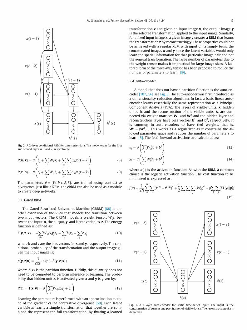
Fig. 2. A 2-layer conditional RBM for time-series data. The model order for the firstand second layer is 3 and 2, respectively.

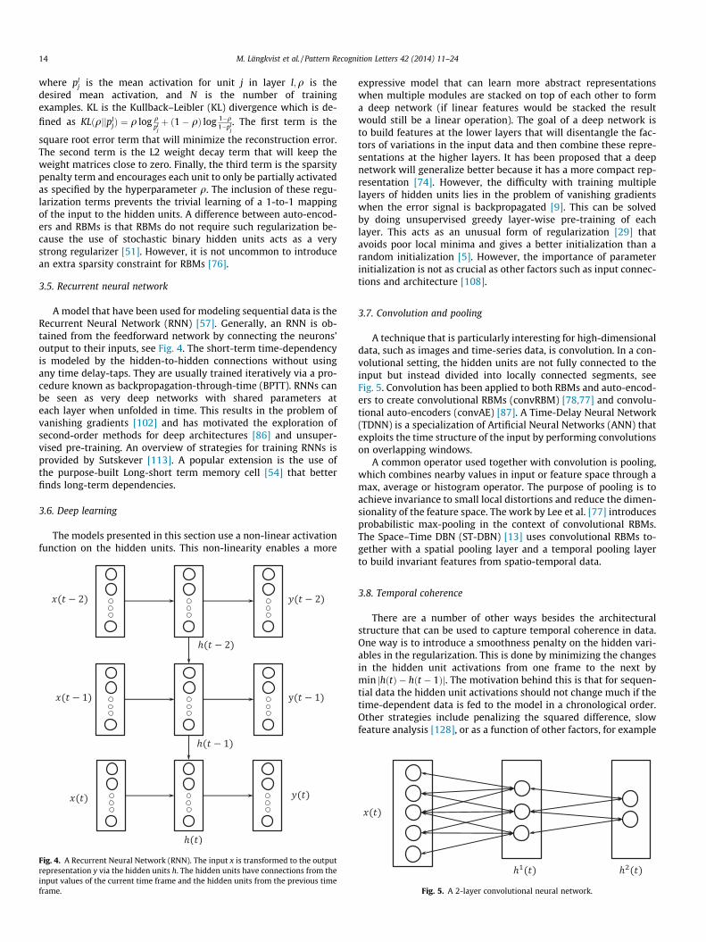
Fig. 3. A 1-layer auto-encoder for static time-series input. The input is theconcatenation of current and past frames of visible data x. The reconstruction of x isdenoted x.

M. Längkvist et al. / Pattern Recognition Letters 42 (2014) 11–24 13

PðhjjxÞ ¼ r bj þX

i

Wijxi þX

k

Xi

Bijkxiðt � kÞ !

ð8Þ

PðxijhÞ ¼ r ci þX

j

Wijhj þX

k

Xi

Aijkxiðt � kÞ !

ð9Þ

The parameters h ¼ fW; b; c;A;Bg, are trained using contrastivedivergence. Just like a RBM, the cRBM can also be used as a moduleto create deep networks.

3.3. Gated RBM

The Gated Restricted Boltzmann Machine (GRBM) [88] is an-other extension of the RBM that models the transition betweentwo input vectors. The GRBM models a weight tensor, Wijk, be-tween the input, x, the output, y, and latent variables, z. The energyfunction is defined as:

Eðy; z; xÞ ¼ �X

ijk

Wijkxiyjzk �X

k

bkzk �X

j

cjyj ð10Þ

where b and c are the bias vectors for x and y, respectively. The con-ditional probability of the transformation and the output image gi-ven the input image is:

pðy; zjxÞ ¼ 1ZðxÞ expð�Eðy; z; xÞÞ ð11Þ

where ZðxÞ is the partition function. Luckily, this quantity does notneed to be computed to perform inference or learning. The proba-bility that hidden unit zi is activated given x and y is given by:

Pðzk ¼ 1jx; yÞ ¼ rX

ij

Wijkxiyj þ bk

!ð12Þ

Learning the parameters is performed with an approximation meth-od of the gradient called contrastive divergence [50]. Each latentvariable zk learns a simple transformation that together are com-bined the represent the full transformation. By fixating a learned

transformation z and given an input image x, the output image yis the selected transformation applied to the input image. Similarly,for a fixed input image x, a given image y creates a RBM that learnsthe transformation z by reconstructing y. These properties could notbe achieved with a regular RBM with input units simply being theconcatenated images x and y since the latent variables would onlylearn the spatial information for that particular image pair and notthe general transformation. The large number of parameters due tothe weight tensor makes it impractical for large image sizes. A fac-tored form of the three-way tensor has been proposed to reduce thenumber of parameters to learn [89].

3.4. Auto-encoder

A model that does not have a partition function is the auto-en-coder [107,7,4], see Fig. 3. The auto-encoder was first introduced asa dimensionality reduction algorithm. In fact, a basic linear auto-encoder learns essentially the same representation as a PrincipalComponent Analysis (PCA). The layers of visible units, x, hiddenunits, h, and the reconstruction of the visible units, x, are con-nected via weight matrices W1 and W2 and the hidden layer andreconstruction layer have bias vectors b1 and b2, respectively. Itis common in auto-encoders to have tied weights, that is,W2 ¼ ðW1ÞT . This works as a regularizer as it constrains the al-lowed parameter space and reduces the number of parameters tolearn [5]. The feed-forward activations are calculated as:

hj ¼ rX

i

W1jixi þ b1

j

!ð13Þ

xi ¼ rX

j

W2ijhj þ b2

i

!ð14Þ

where rð�Þ is the activation function. As with the RBM, a commonchoice is the logistic activation function. The cost function to beminimized is expressed as:

JðhÞ ¼ 12N

XN

n

Xi

ðxðnÞi � xiðnÞÞ

2þ k

2

Xl

Xi

Xj

ðWlijÞ

2þ bX

l

Xj

KLðqjjpljÞ

ð15Þ

14 M. Längkvist et al. / Pattern Recognition Letters 42 (2014) 11–24

where plj is the mean activation for unit j in layer l;q is the

desired mean activation, and N is the number of trainingexamples. KL is the Kullback–Leibler (KL) divergence which is de-fined as KLðqjjpl

jÞ ¼ q log qpl

jþ ð1� qÞ log 1�q

1�plj. The first term is the

square root error term that will minimize the reconstruction error.The second term is the L2 weight decay term that will keep theweight matrices close to zero. Finally, the third term is the sparsitypenalty term and encourages each unit to only be partially activatedas specified by the hyperparameter q. The inclusion of these regu-larization terms prevents the trivial learning of a 1-to-1 mappingof the input to the hidden units. A difference between auto-encod-ers and RBMs is that RBMs do not require such regularization be-cause the use of stochastic binary hidden units acts as a verystrong regularizer [51]. However, it is not uncommon to introducean extra sparsity constraint for RBMs [76].

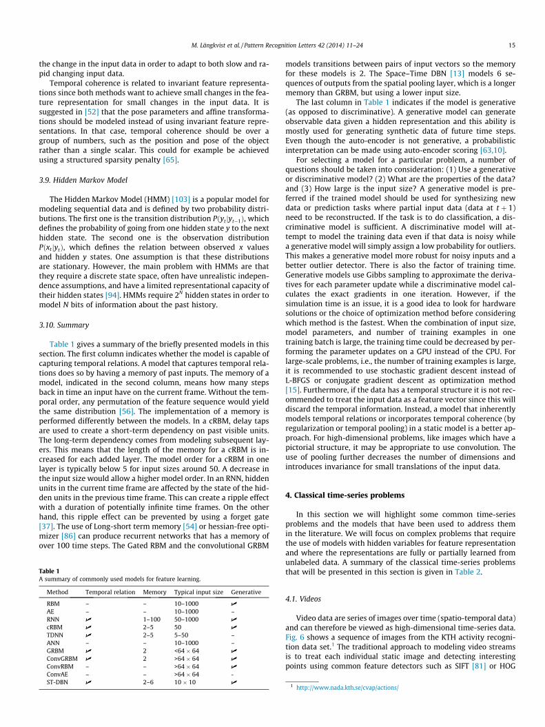
3.5. Recurrent neural network

A model that have been used for modeling sequential data is theRecurrent Neural Network (RNN) [57]. Generally, an RNN is ob-tained from the feedforward network by connecting the neurons’output to their inputs, see Fig. 4. The short-term time-dependencyis modeled by the hidden-to-hidden connections without usingany time delay-taps. They are usually trained iteratively via a pro-cedure known as backpropagation-through-time (BPTT). RNNs canbe seen as very deep networks with shared parameters ateach layer when unfolded in time. This results in the problem ofvanishing gradients [102] and has motivated the exploration ofsecond-order methods for deep architectures [86] and unsuper-vised pre-training. An overview of strategies for training RNNs isprovided by Sutskever [113]. A popular extension is the use ofthe purpose-built Long-short term memory cell [54] that betterfinds long-term dependencies.

3.6. Deep learning

The models presented in this section use a non-linear activationfunction on the hidden units. This non-linearity enables a more

Fig. 4. A Recurrent Neural Network (RNN). The input x is transformed to the outputrepresentation y via the hidden units h. The hidden units have connections from theinput values of the current time frame and the hidden units from the previous timeframe.

expressive model that can learn more abstract representationswhen multiple modules are stacked on top of each other to forma deep network (if linear features would be stacked the resultwould still be a linear operation). The goal of a deep network isto build features at the lower layers that will disentangle the fac-tors of variations in the input data and then combine these repre-sentations at the higher layers. It has been proposed that a deepnetwork will generalize better because it has a more compact rep-resentation [74]. However, the difficulty with training multiplelayers of hidden units lies in the problem of vanishing gradientswhen the error signal is backpropagated [9]. This can be solvedby doing unsupervised greedy layer-wise pre-training of eachlayer. This acts as an unusual form of regularization [29] thatavoids poor local minima and gives a better initialization than arandom initialization [5]. However, the importance of parameterinitialization is not as crucial as other factors such as input connec-tions and architecture [108].

3.7. Convolution and pooling

A technique that is particularly interesting for high-dimensionaldata, such as images and time-series data, is convolution. In a con-volutional setting, the hidden units are not fully connected to theinput but instead divided into locally connected segments, seeFig. 5. Convolution has been applied to both RBMs and auto-encod-ers to create convolutional RBMs (convRBM) [78,77] and convolu-tional auto-encoders (convAE) [87]. A Time-Delay Neural Network(TDNN) is a specialization of Artificial Neural Networks (ANN) thatexploits the time structure of the input by performing convolutionson overlapping windows.

A common operator used together with convolution is pooling,which combines nearby values in input or feature space through amax, average or histogram operator. The purpose of pooling is toachieve invariance to small local distortions and reduce the dimen-sionality of the feature space. The work by Lee et al. [77] introducesprobabilistic max-pooling in the context of convolutional RBMs.The Space–Time DBN (ST-DBN) [13] uses convolutional RBMs to-gether with a spatial pooling layer and a temporal pooling layerto build invariant features from spatio-temporal data.

3.8. Temporal coherence

There are a number of other ways besides the architecturalstructure that can be used to capture temporal coherence in data.One way is to introduce a smoothness penalty on the hidden vari-ables in the regularization. This is done by minimizing the changesin the hidden unit activations from one frame to the next bymin jhðtÞ � hðt � 1Þj. The motivation behind this is that for sequen-tial data the hidden unit activations should not change much if thetime-dependent data is fed to the model in a chronological order.Other strategies include penalizing the squared difference, slowfeature analysis [128], or as a function of other factors, for example

Fig. 5. A 2-layer convolutional neural network.

M. Längkvist et al. / Pattern Recognition Letters 42 (2014) 11–24 15

the change in the input data in order to adapt to both slow and ra-pid changing input data.

Temporal coherence is related to invariant feature representa-tions since both methods want to achieve small changes in the fea-ture representation for small changes in the input data. It issuggested in [52] that the pose parameters and affine transforma-tions should be modeled instead of using invariant feature repre-sentations. In that case, temporal coherence should be over agroup of numbers, such as the position and pose of the objectrather than a single scalar. This could for example be achievedusing a structured sparsity penalty [65].

3.9. Hidden Markov Model

The Hidden Markov Model (HMM) [103] is a popular model formodeling sequential data and is defined by two probability distri-butions. The first one is the transition distribution Pðyt jyt�1Þ, whichdefines the probability of going from one hidden state y to the nexthidden state. The second one is the observation distributionPðxtjytÞ, which defines the relation between observed x valuesand hidden y states. One assumption is that these distributionsare stationary. However, the main problem with HMMs are thatthey require a discrete state space, often have unrealistic indepen-dence assumptions, and have a limited representational capacity oftheir hidden states [94]. HMMs require 2N hidden states in order tomodel N bits of information about the past history.

3.10. Summary

Table 1 gives a summary of the briefly presented models in thissection. The first column indicates whether the model is capable ofcapturing temporal relations. A model that captures temporal rela-tions does so by having a memory of past inputs. The memory of amodel, indicated in the second column, means how many stepsback in time an input have on the current frame. Without the tem-poral order, any permutation of the feature sequence would yieldthe same distribution [56]. The implementation of a memory isperformed differently between the models. In a cRBM, delay tapsare used to create a short-term dependency on past visible units.The long-term dependency comes from modeling subsequent lay-ers. This means that the length of the memory for a cRBM is in-creased for each added layer. The model order for a cRBM in onelayer is typically below 5 for input sizes around 50. A decrease inthe input size would allow a higher model order. In an RNN, hiddenunits in the current time frame are affected by the state of the hid-den units in the previous time frame. This can create a ripple effectwith a duration of potentially infinite time frames. On the otherhand, this ripple effect can be prevented by using a forget gate[37]. The use of Long-short term memory [54] or hessian-free opti-mizer [86] can produce recurrent networks that has a memory ofover 100 time steps. The Gated RBM and the convolutional GRBM

Table 1A summary of commonly used models for feature learning.

Method Temporal relation Memory Typical input size Generative

RBM – – 10–1000 U

AE – – 10–1000 –RNN U 1–100 50–1000 U

cRBM U 2–5 50 U

TDNN U 2–5 5–50 –ANN – – 10–1000 –GRBM U 2 <64 � 64 U

ConvGRBM U 2 >64 � 64 U

ConvRBM – – >64 � 64 U

ConvAE – – >64 � 64 -ST-DBN U 2–6 10 � 10 U

models transitions between pairs of input vectors so the memoryfor these models is 2. The Space–Time DBN [13] models 6 se-quences of outputs from the spatial pooling layer, which is a longermemory than GRBM, but using a lower input size.

The last column in Table 1 indicates if the model is generative(as opposed to discriminative). A generative model can generateobservable data given a hidden representation and this ability ismostly used for generating synthetic data of future time steps.Even though the auto-encoder is not generative, a probabilisticinterpretation can be made using auto-encoder scoring [63,10].

For selecting a model for a particular problem, a number ofquestions should be taken into consideration: (1) Use a generativeor discriminative model? (2) What are the properties of the data?and (3) How large is the input size? A generative model is pre-ferred if the trained model should be used for synthesizing newdata or prediction tasks where partial input data (data at t þ 1)need to be reconstructed. If the task is to do classification, a dis-criminative model is sufficient. A discriminative model will at-tempt to model the training data even if that data is noisy whilea generative model will simply assign a low probability for outliers.This makes a generative model more robust for noisy inputs and abetter outlier detector. There is also the factor of training time.Generative models use Gibbs sampling to approximate the deriva-tives for each parameter update while a discriminative model cal-culates the exact gradients in one iteration. However, if thesimulation time is an issue, it is a good idea to look for hardwaresolutions or the choice of optimization method before consideringwhich method is the fastest. When the combination of input size,model parameters, and number of training examples in onetraining batch is large, the training time could be decreased by per-forming the parameter updates on a GPU instead of the CPU. Forlarge-scale problems, i.e., the number of training examples is large,it is recommended to use stochastic gradient descent instead ofL-BFGS or conjugate gradient descent as optimization method[15]. Furthermore, if the data has a temporal structure it is not rec-ommended to treat the input data as a feature vector since this willdiscard the temporal information. Instead, a model that inherentlymodels temporal relations or incorporates temporal coherence (byregularization or temporal pooling) in a static model is a better ap-proach. For high-dimensional problems, like images which have apictorial structure, it may be appropriate to use convolution. Theuse of pooling further decreases the number of dimensions andintroduces invariance for small translations of the input data.

4. Classical time-series problems

In this section we will highlight some common time-seriesproblems and the models that have been used to address themin the literature. We will focus on complex problems that requirethe use of models with hidden variables for feature representationand where the representations are fully or partially learned fromunlabeled data. A summary of the classical time-series problemsthat will be presented in this section is given in Table 2.

4.1. Videos

Video data are series of images over time (spatio-temporal data)and can therefore be viewed as high-dimensional time-series data.Fig. 6 shows a sequence of images from the KTH activity recogni-tion data set.1 The traditional approach to modeling video streamsis to treat each individual static image and detecting interestingpoints using common feature detectors such as SIFT [81] or HOG

1 http://www.nada.kth.se/cvap/actions/

Table 2A summary of commonly used time-series problems.

Problem Multi-variate Raw data Frequency rich Common features Common method Benchmark set

Stock prediction – U – – ANN DJIAVideo U U – SIFT, HOG ConvRBM KTHSpeech Recognition – (U) U MFCC RBM, RNN TIMITMusic recognition U – U Chroma, MFCC ConvRBM GTZANMotion capture U U – – cRBM CMUE-nose U U – Many TDNN –Physiological data U (U) U Many, spectogram RBM, AE PhysioNET

Fig. 6. Four images from the KTH action recognition data set of a person running at frame 100, 105, 110, and 115. The KTH data set also contains videos of walking, jogging,boxing, hand waving, and handclapping.

16 M. Längkvist et al. / Pattern Recognition Letters 42 (2014) 11–24

[24]. These features are domain-specific for static images and are noteasily extended to other domains such as video [73].

The approach taken by Stavens and Thrun [111] learns its owndomain-optimized features instead of using pre-defined features,but still from static images. A better approach to modeling videosis to learn image transitions instead of working with static images.A Gated Restricted Boltzmann Machine (GRBM) [88] has been usedfor this purpose where the input, x, of the GRBM is the full image inone time frame and the output y is the full image in the subsequenttime frame. However, since the network is fully connected to theimage the method does not scale well to larger images and localtransformations at multiple locations must be re-learned.

A convolutional version of the GRBM using probabilistic max-pooling is presented by Taylor et al. [116]. The use of convolutionreduces the number of parameters to learn, allows for larger inputsizes, and better handles the local affine transformations that canappear anywhere in the image. The model was validated on syn-thetic data and a number of benchmark data sets, including theKTH activity recognition data set.

The work by Le et al. [73] presents an unsupervised spatio-tem-poral feature learning method using an extension of IndependentSubspace Analysis (ISA) [60]. The extensions include hierarchical(stacked) convolutional ISA modules together with pooling. A dis-advantage of ISA is that it does not scale well to large input sizes.The inclusion of convolution and stacking solves this problem bylearning on smaller patches of input data. The method is validatedon a number of benchmark sets, including KTH. One advantage ofthe method is that the use of ISA reduces the need for tweakingmany of the hyperparameters seen in RBM-based methods, suchas learning rate, weight decay, convergence parameters, etc.

Modeling temporal relations in video have also been done usingtemporal pooling. The work by Chen and de Freitas [13] uses con-volutional RBMs as building blocks for spatial pooling and thenperforms temporal pooling on the spatial pooling units. The meth-od is called Space–Time Deep Belief Network (ST-DBN). The ST-DBN allows for invariance and statistical dependencies in bothspace and time. The method achieved superior performance onapplications such as action recognition and video denoising whencompared to a standard convolutional DBN.

The use of temporal coherence for modeling videos is done byZou et al. [135], where an auto-encoder with a L1-cost on the

temporal difference on the pooling units is used to learn featuresthat improve object recognition on still images. The work byHyvärinen [58] also uses temporal information as a criterion forlearning representations.

The use of deep learning, feature learning, and convolution withpooling has propelled the advances in video processing. Modelingstreams of video is a natural continuation for deep learning algo-rithms since they have already been shown to be successful atbuilding useful features from static images. By focusing on learningtemporal features in videos, the performance on static images canbe improved, which motivates the need for continuing developingdeep learning algorithms that capture temporal relations. The earlyattempts at extending deep learning algorithms to video data wasdone by modeling the transition between two frames. The use oftemporal pooling extends the time-dependencies a model canlearn beyond a single frame transition. However, the time-depen-dency that has been modeled is still just a few frames. A possiblefuture direction for video processing is to look at models that canlearn longer time-dependencies.

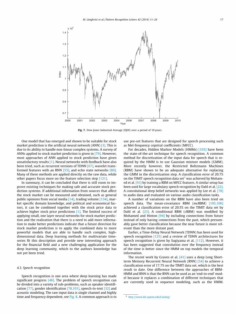
4.2. Stock market prediction

Stock market data are highly complex and difficult to predict,even for human experts, due to a number of external factors, e.g.,politics, global economy, and trader expectation. The trends instock market data tend to be nonlinear, uncertain, and non-station-ary. Fig. 7 shows the Dow Jones Industrial Average (DJOI) over adecade. According to the Efficient Market Hypothesis (EMH) [30],stock market prices follow a random walk pattern, meaning thata stock has the same probability to go up as it has to go down,resulting in that predictions can not have more than 50% accuracy[121]. The EMH state that stock prices are largely driven by ‘‘news’’rather than present and past prices. However, it has also been ar-gued that stock market prices do not follow a random walk andthat they can be predicted [84]. The landscape for acquiring bothnews and stock information looks very different today than it diddecades ago. As an example, it has been shown that predicted stockprices can be improved if further information is extracted from on-line social media, such as Twitter feeds [14] and online chat activ-ity [43].

2000 2001 2002 2003 2004 2006 2007 2008 2009 2010

0.7

0.8

0.9

1

1.1

1.2

1.3

1.4

x 104

Year

Inde

x

Fig. 7. Dow Jones Industrial Average (DJOI) over a period of 10 years.

M. Längkvist et al. / Pattern Recognition Letters 42 (2014) 11–24 17

One model that has emerged and shown to be suitable for stockmarket prediction is the artificial neural network (ANN) [3]. This isdue to its ability to handle non-linear complex systems. A survey ofANNs applied to stock market prediction is given in [79]. However,most approaches of ANN applied to stock prediction have givenunsatisfactory results [1]. Neural networks with feedback have alsobeen tried, such as recurrent versions of TDNN [67], wavelet trans-formed features with an RNN [55], and echo state networks [80].Many of these methods are applied directly on the raw data, whileother papers focus more on the feature selection step [121].

In summary, it can be concluded that there is still room to im-prove existing techniques for making safe and accurate stock pre-diction systems. If additional information from sources that affectthe stock market can be measured and obtained, such as generalpublic opinions from social media [14], trading volume [134], mar-ket specific domain knowledge, and political and economical fac-tors, it can be combined together with the stock price data toachieve higher stock price predictions [1]. The limited success ofapplying small, one layer neural networks for stock market predic-tion and the realization that there is a need to add more informa-tion to make better predictions indicate that a future direction forstock market prediction is to apply the combined data to morepowerful models that are able to handle such complex, high-dimensional data. Deep learning methods for multivariate time-series fit this description and provide new interesting approachfor the financial field and a new challenging application for thedeep learning community, which to the authors knowledge hasnot yet been tried.

2 http://www.ldc.upenn.edu/Catalog/

4.3. Speech recognition

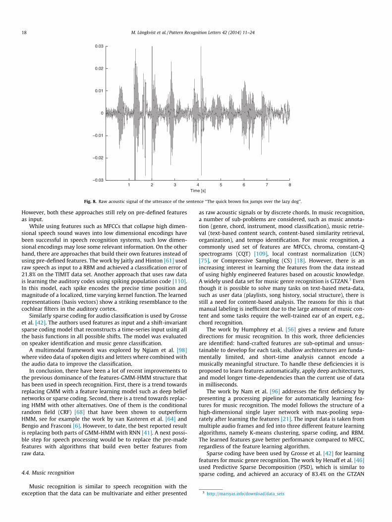
Speech recognition is one area where deep learning has madesignificant progress [48]. The problem of speech recognition canbe divided into a variety of sub-problems, such as speaker identifi-cation [77], gender identification [78,101], speech-to-text [32] andacoustic modeling. The raw input data is single channel and highlytime and frequency dependent, see Fig. 8. A common approach is to

use pre-set features that are designed for speech processing suchas Mel-frequency cepstral coefficients (MFCC).

For decades, Hidden Markov Models (HMMs) [103] have beenthe state-of-the-art technique for speech recognition. A commonmethod for discretization of the input data for speech that is re-quired by the HMM is to use Gaussian mixture models (GMM).More recently however, the Restricted Boltzmann Machines(RBM) have shown to be an adequate alternative for replacingthe GMM in the discretization step. A classification error of 20.7%on the TIMIT speech recognition data set2 was achieved by Moham-ed et al. [93] by training a RBM on MFCC features. A similar setup hasbeen used for large vocabulary speech recognition by Dahl et al. [22].A convolutional deep belief networks was applied by Lee et al. [78]to audio data and evaluated on various audio classification tasks.

A number of variations on the RBM have also been tried onspeech data. The mean-covariance RBM (mcRBM) [105,106]achieved a classification error of 20.5% on the TIMIT data set byDahl et al. [23]. A conditional RBM (cRBM) was modified byMohamed and Hinton [94] by including connections from futureinstead of only having connections from the past, which presum-ably gave better classification because the near future is more rel-evant than the more distant past.

Earlier, a Time-Delay Neural Network (TDNN) has been used forspeech recognition [125] and a review of TDNN architectures forspeech recognition is given by Sugiyama et al. [112]. However, ithas been suggested that convolution over the frequency insteadof the time is better since the HMM on top models the temporalinformation.

The recent work by Graves et al. [41] uses a deep Long Short-term Memory Recurrent Neural Network (RNN) [54] to achieve aclassification error of 17.7% on the TIMIT data set, which is the bestresult to date. One difference between the approaches of RBM-HMM and RNN is that the RNN can be used as an ‘end-to-end’ mod-el because it replaces a combination of different techniques thatare currently used in sequence modeling, such as the HMM.

1 2 3 4 5 6 7 8−0.03

−0.02

−0.01

0

0.01

0.02

0.03

Time [s]

Fig. 8. Raw acoustic signal of the utterance of the sentence ‘‘The quick brown fox jumps over the lazy dog’’.

18 M. Längkvist et al. / Pattern Recognition Letters 42 (2014) 11–24

However, both these approaches still rely on pre-defined featuresas input.

While using features such as MFCCs that collapse high dimen-sional speech sound waves into low dimensional encodings havebeen successful in speech recognition systems, such low dimen-sional encodings may lose some relevant information. On the otherhand, there are approaches that build their own features instead ofusing pre-defined features. The work by Jaitly and Hinton [61] usedraw speech as input to a RBM and achieved a classification error of21.8% on the TIMIT data set. Another approach that uses raw datais learning the auditory codes using spiking population code [110].In this model, each spike encodes the precise time position andmagnitude of a localized, time varying kernel function. The learnedrepresentations (basis vectors) show a striking resemblance to thecochlear filters in the auditory cortex.

Similarly sparse coding for audio classification is used by Grosseet al. [42]. The authors used features as input and a shift-invariantsparse coding model that reconstructs a time-series input using allthe basis functions in all possible shifts. The model was evaluatedon speaker identification and music genre classification.

A multimodal framework was explored by Ngiam et al. [98]where video data of spoken digits and letters where combined withthe audio data to improve the classification.

In conclusion, there have been a lot of recent improvements tothe previous dominance of the features-GMM-HMM structure thathas been used in speech recognition. First, there is a trend towardsreplacing GMM with a feature learning model such as deep beliefnetworks or sparse coding. Second, there is a trend towards replac-ing HMM with other alternatives. One of them is the conditionalrandom field (CRF) [68] that have been shown to outperformHMM, see for example the work by van Kasteren et al. [64] andBengio and Frasconi [6]. However, to date, the best reported resultis replacing both parts of GMM-HMM with RNN [41]. A next possi-ble step for speech processing would be to replace the pre-madefeatures with algorithms that build even better features fromraw data.

3 http://marsyas.info/download/data_sets

4.4. Music recognition

Music recognition is similar to speech recognition with theexception that the data can be multivariate and either presented

as raw acoustic signals or by discrete chords. In music recognition,a number of sub-problems are considered, such as music annota-tion (genre, chord, instrument, mood classification), music retrie-val (text-based content search, content-based similarity retrieval,organization), and tempo identification. For music recognition, acommonly used set of features are MFCCs, chroma, constant-Qspectrograms (CQT) [109], local contrast normalization (LCN)[75], or Compressive Sampling (CS) [18]. However, there is anincreasing interest in learning the features from the data insteadof using highly engineered features based on acoustic knowledge.A widely used data set for music genre recognition is GTZAN.3 Eventhough it is possible to solve many tasks on text-based meta-data,such as user data (playlists, song history, social structure), there isstill a need for content-based analysis. The reasons for this is thatmanual labeling is inefficient due to the large amount of music con-tent and some tasks require the well-trained ear of an expert, e.g.,chord recognition.

The work by Humphrey et al. [56] gives a review and futuredirections for music recognition. In this work, three deficienciesare identified: hand-crafted features are sub-optimal and unsus-tainable to develop for each task, shallow architectures are funda-mentally limited, and short-time analysis cannot encode amusically meaningful structure. To handle these deficiencies it isproposed to learn features automatically, apply deep architectures,and model longer time-dependencies than the current use of datain milliseconds.

The work by Nam et al. [96] addresses the first deficiency bypresenting a processing pipeline for automatically learning fea-tures for music recognition. The model follows the structure of ahigh-dimensional single layer network with max-pooling sepa-rately after learning the features [21]. The input data is taken frommultiple audio frames and fed into three different feature learningalgorithms, namely K-means clustering, sparse coding, and RBM.The learned features gave better performance compared to MFCC,regardless of the feature learning algorithm.

Sparse coding have been used by Grosse et al. [42] for learningfeatures for music genre recognition. The work by Henaff et al. [46]used Predictive Sparse Decomposition (PSD), which is similar tosparse coding, and achieved an accuracy of 83.4% on the GTZAN

4 http://mocap.cs.cmu.edu/

M. Längkvist et al. / Pattern Recognition Letters 42 (2014) 11–24 19

data. In this work, the features are automatically learned from CTQspectograms in an unsupervised manner. The learned features cap-ture information about which chords are being played in a partic-ular frame and produce comparable results to hand-craftedfeatures for the task of genre recognition. A limitation, however,is that it ignores temporal dependencies between frames.

Convolutional DBNs were used by Lee et al. [78] to learn fea-tures from speech and music spectrograms and from engineeredfeatures by Dieleman [25]. The work by Hamel and Eck [45] alsouses convolutional DBN to achieve an accuracy of 84.3% on theGTZAN dataset.

Self-taught learning have also been used for music genre classi-fication. The self-taught learning framework attempts to use unla-beled data that does not share the labels of the classification task toimprove classification performance [104,62]. Self-taught learningand sparse coding are used by Markov and Matsui [85] where unla-beled data from other music genres other than in the classificationtask was used to train the model.

In conclusion, there are many works that use unsupervised fea-ture learning methods for music recognition. The motivation forusing deep networks is that music itself is structured hierarchicallyby a combination of chords, melodies and rhythms that createsmotives, phrases, sections and finally entire pieces [56]. Just likein speech recognition, the input data is often in some form of spec-trograms. Many works leave the natural step of learning featuresfrom raw data as future work [95]. Still, as proposed by Humphreyet al. [56], even though convolutional networks have given goodresults on time-frequency representations of audio, there is roomfor discovering new and better models.

4.5. Motion capture data

Modeling human motion has several applications such as track-ing, activity recognition, style and content separation, person iden-tification, computer animation, and synthesis of new motion data.Motion capture data is collected from recordings of movementsfrom several points on the body of a human actor. These pointscan be captured by cameras that either track the position of strate-gically placed markers (usually at joint centers) or uses vision-based algorithms for tracking points of interest [38]. The pointsare represented as 3D Cartesian coordinates over time and are usedto form a skeletal structure with constant limb lengths by translat-ing the points to relative joint angles. The joint angles can be ex-pressed in Euler angles, 4D quaternions, or exponential mapparameterization [40] and can have 1–3 degrees of freedom(DOF) each. The full data set consists of the orientation and trans-lation of the root and all relative joint angles for each time frame aswell as the constant skeleton model. The data is noisy, high-dimen-sional, and multivariate with complex nonlinear relationships. Ithas a lower frequency compared to speech and music data andsome of the signals may be task-redundant.

Some of the traditional approaches include the work by Brandand Hertzmann [16], which models both the style and content ofhuman motion using Hidden Markov Models (HMMs). The differ-ent styles were learned from unlabeled data and the trained modelwas used to synthesize motion data. A linear dynamical systemswas used by Chiappa et al. [20] to model three different motionsof a human performing the task of holding a cup that has a ball at-tached to it with a string and then try to catch the ball into the cup(game of Balero). A Bayesian mixture of linear Gaussian state-spacemodels (LGSSM) was trained with data from a human learner andused to generate new motions that was clustered and simulated ona robotic manipulator.

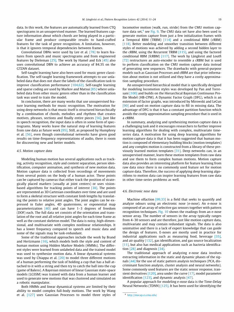
Both HMMs and linear dynamical systems are limited by theirability to model complex full-body motions. The work by Wanget al. [127] uses Gaussian Processes to model three styles of

locomotive motion (walk, run, stride) from the CMU motion cap-ture data set,4 see Fig. 9. The CMU data set have also been used togenerate motion capture from just a few initialization frames witha Temporal RBM (TRBM) [114] and a conditional RBM (cRBM)[118]. Better modeling and smoother transition between differentstyles of motions was achieved by adding a second hidden layer tothe cRBM, using the Recurrent TRBM [115], and using the factoredconditional RBM (fcRBM) [117]. The work by Längkvist and Loutfi[72] restructures an auto-encoder to resemble a cRBM but is usedto perform classification on the CMU motion capture data insteadof generating new sequences. The drawbacks with general-purposemodels such as Gaussian Processes and cRBM are that prior informa-tion about motion is not utilized and they have a costly approxima-tion sampling procedure.

An unsupervised hierarchical model that is specifically designedfor modeling locomotion styles was developed by Pan and Torre-sani [100] and builds on the Hierarchical Bayesian Continuous Pro-file Model (HB-CPM). A Dynamic Factor Graph (DFG), which is anextension of factor graphs, was introduced by Mirowski and LeCun[90] and used on motion capture data to fill in missing data. Theadvantage of DFG is that it has a constant partition function whichavoids the costly approximation sampling procedure that is used ina cRBM.

In summary, analyzing and synthesizing motion capture data isa challenging task and it encourages researchers to further improvelearning algorithms for dealing with complex, multivariate time-series data. A motivation for using deep learning algorithms formotion capture data is that it has been suggested that human mo-tion is composed of elementary building blocks (motion templates)and any complex motion is constructed from a library of these pre-viously learned motion templates [31]. Deep networks can, in anunsupervised manner, learn these motion templates from raw dataand use them to form complex human motions. Motion capturedata also provides an interesting platform for feature learning fromraw data since there is no commonly used feature set for motioncapture data. Therefore, the success of applying deep learning algo-rithms to motion data can inspire learning features from raw datain other time-series problems as well.

4.6. Electronic nose data

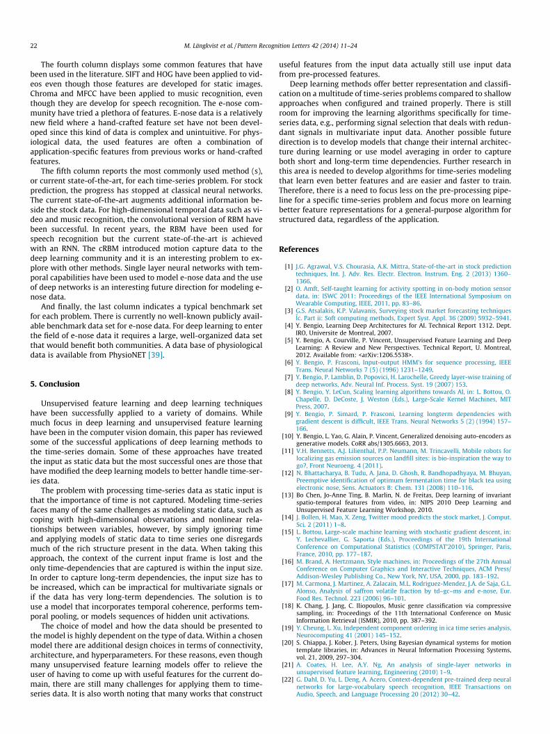
Machine olfaction [99,33] is a field that seeks to quantify andanalyze odours using an electronic nose (e-nose). An e-nose iscomposed of an array of selective gas sensors together with patternrecognition techniques. Fig. 10 shows the readings from an e-nosesensor array. The number of sensors in the array typically rangesfrom 4–30 sensors and are therefore, just like motion capture data,multivariate and may contain redundant signals. The data is alsounintuitive and there is a lack of expert knowledge that can guidethe design of features. E-noses are mostly used in practice forindustrial applications such as measuring food, beverage [35],and air quality [132], gas identification, and gas source localization[11], but also has medical applications such as bacteria identifica-tion [28] and diagnosis [34].

The traditional approach of analyzing e-nose data involvesextracting information in the static and dynamic phases of the sig-nals [44] for the use of static pattern analysis techniques (PCA, dis-criminant function analysis, cluster analysis and neural networks).Some commonly used features are the static sensor response, tran-sient derivatives [120], area under the curve [17], model parameteridentification [123], and dynamic analysis [47].

A popular approach for modeling e-nose data is the Time-DelayNeural Networks (TDNN) [125]. It has been used for identifying the

−20

0

20

Position

−10

−5

0

5

Rotation

−5

0

5

10

Lower back

−6

−4

−2

0

2

Upper back

−6

−4

−2

0

2

Thorax

−15

−10

−5

0

Lower neck

−15

−10

−5

0

5

Upper neck

−2

0

2

Head

−5

0

5

x 10−14 Clavicle

−80−60−40−20

020

Humerus

70

80

90

100

110

Radius

−10

0

10

20

30

Wrist

−40

−20

0

20

40

Hand

6.5

7

7.5

8

Finger

−10

0

10

20

Thumb

−5

0

5

x 10−14 Clavicle 2

−50

0

50

100Humerus 2

−30

−20

−10

0

10 Hand 2

0

20

40Thumb 2

−40

−20

0

20

Femur

40

60

80

100

Libia

−20

−10

0

10

Foot

−30

−20

−10

0

Toes

−40

−20

0

Femur 2

−20

0

20

Foot 2

Fig. 9. A sequence of human motion from the CMU motion capture data set.

10 20 30 40 50 60 700

0.1

0.2

0.3

0.4

0.5

0.6

0.7

0.8

Sample [0.5 Hz]

Sen

sor

valu

e

Fig. 10. Normalized data from an array of electronic nose sensors.

20 M. Längkvist et al. / Pattern Recognition Letters 42 (2014) 11–24

smell of spices [133], ternary mixtures [124], optimum fermenta-tion time for black tea [12], and vintages of wine [130]. An RNNhave been used for odour localization with a mobile robot [27].

The work by Vembu et al. [123] compares the gas discrimina-tion and localization between three approaches: SVM on raw data,SVM on features extracted from auto-regressive and linear dynam-ical systems, and finally a SVMs with kernels specialized for struc-tured data [36]. The SVM with built-in time-aware kernelsperformed better than techniques that used feature extraction,even though the features captured temporal information.

More recently, an auto-encoder, RBM, and cRBM have been usedfor bacteria identification [71] and fast classification of meat spoil-age markers [69].

E-nose data introduces the challenge of improving models thatcan deal with redundant signals. It is not feasible to produce tailor-made sensors for each possible individual gas and combinations ofgases of interest. Therefore the common approach is to use an ar-ray of sensors with different properties and leave the discrimina-tion to the pattern analysis software. It is also not desirable toconstruct new feature sets for each e-nose application so a data-driven feature learning method is useful. The early works on e-nose data create feature vectors of simple features for each signalsuch as the static response or the slope of dynamic response andthen feed it to a classifier. Recently, the use of dynamic modelssuch as neural networks with tapped delays and SVMs with kernelsfor structured data have shown to improve the performance overstatic approaches. The next step is to continue this trend of usingdynamical models that constructs robust features that can dealwith noisy inputs in order to quantify and classify odors in more

M. Längkvist et al. / Pattern Recognition Letters 42 (2014) 11–24 21

challenging open environments with many different simultaneousgas sources.

4.7. Physiological data

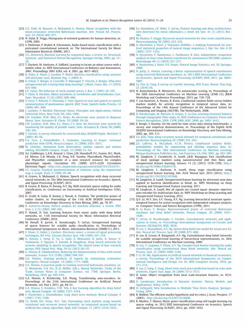
With physiological data we consider recordings such as electro-encephalography (EEG), magnetoencephalography (MEG), electro-cardiography (ECG), and wearable sensors for health monitoring.Fig. 11 shows an example of how physiological data look like.The data can exist both as singular or multiple channels. The useof a feature learning algorithm is particularly beneficial in medicalapplications because acquiring a labeled medical data set is expen-sive since the data sets are often very large and require the labelingof an expert in the field.

The work by Mirowski et al. [92] compares convolutional net-works with logistic regression and SVMs for epileptic seizure pre-diction from intracranial EEG signals. The features that are used arehand-engineered bi-variate features between channels that encoderelationship between pairs of EEG channels. The result was thatconvolutional networks achieved only 1 false-alarm predictionfrom 21 patients while the SVM had 10 false-alarms. TDNN andICA has also been used for EEG-based prediction of epileptic sei-zures [91]. The application of self-organizing maps (SOM) to ana-lyze EMG data is presented by Tucker [122].

A RBM-based method that builds features from raw data forsleep stage classification from 4-channel polysomnography datahas been proposed by Längkvist et al. [70]. A similar setup wasused by Wulsin et al. [129] for modeling single channel EEG wave-forms used for anomaly detection. A DBN is used by Wang andShang [126] to automatically extract features from raw unlabeledphysiological data and achieves better classification than a fea-ture-based approach. These recent works show that DBNs can beapplied to raw physiological data to effectively learn relevantfeatures.

A source separation method tailor-made to EEG and MEG sig-nals is proposed by Hyvärinen et al. [59]. The data is preprocessedby short-time Fourier transforms and then fed to an ICA. The workshows that temporal correlations are adequately taken into ac-count. Independent Component Analysis (ICA) has provided to bea new tool to analyze time series and is a unifying framework that

0 5 10 1

EMG

EOG2

EOG1

EEG2

EEG1

Tim

Fig. 11. Data from EEG (top two signals), EOG (third and fourth signal), and

combines sparseness, temporal coherence, topography and com-plex cell pooling in a single model [58]. A method for how to orderthe independent components for time-series is explored by Cheungand Xu [19].

Self-taught learning has been used with time-series data fromwearable hand-motion sensors [2].

The field of physiological data is large and many different meth-ods have been used. The characteristics of physiological data couldbe particularly interesting for the deep learning community be-cause it can be used to explore the feasibility of learning featuresfrom raw data, which hopefully can inspire similar approaches inother time-series domains.

4.8. Summary

Table 2 gives a summary of the time-series problems that havebeen presented in this section. The first column indicates if thedata is multivariate (or only contains one signal, univariate). Stockprediction is often viewed as a single channel problem, which ex-plains the difficulties to produce accurate prediction systems, sincestocks depend on a myriad of other factors, and arguably not at allon past values of the stock itself. For speech recognition, the use ofmultimodal sources can improve performance [98].

The second column shows which problems have attempted tocreate features purely from raw data. Only a few works have at-tempted this with speech recognition [61,110] and physiologicaldata [129,70,126]. To the authors knowledge, learning featuresfrom raw data has not been attempted in music recognition. Theprocess of constructing features from raw data has been well dem-onstrated for vision-tasks but is cautiously used for time-seriesproblems. Models such as TDNN, cRBM and convolutional RBMsare well suited for being applied to raw data (or slightly pre-pro-cessed data).

The third column indicates which time-series problems havevaluable information in the frequency-domain. For frequency-richproblems, it is uncommon to attempt to learn features from rawdata. A reason for this is that current feature learning algorithmsare yet not well-suited for learning features in the frequency-domain.

5 20 25 30e [s]

EMG (bottom signal), recorded with a polysomnograph during sleep.

22 M. Längkvist et al. / Pattern Recognition Letters 42 (2014) 11–24

The fourth column displays some common features that havebeen used in the literature. SIFT and HOG have been applied to vid-eos even though those features are developed for static images.Chroma and MFCC have been applied to music recognition, eventhough they are develop for speech recognition. The e-nose com-munity have tried a plethora of features. E-nose data is a relativelynew field where a hand-crafted feature set have not been devel-oped since this kind of data is complex and unintuitive. For phys-iological data, the used features are often a combination ofapplication-specific features from previous works or hand-craftedfeatures.

The fifth column reports the most commonly used method (s),or current state-of-the-art, for each time-series problem. For stockprediction, the progress has stopped at classical neural networks.The current state-of-the-art augments additional information be-side the stock data. For high-dimensional temporal data such as vi-deo and music recognition, the convolutional version of RBM havebeen successful. In recent years, the RBM have been used forspeech recognition but the current state-of-the-art is achievedwith an RNN. The cRBM introduced motion capture data to thedeep learning community and it is an interesting problem to ex-plore with other methods. Single layer neural networks with tem-poral capabilities have been used to model e-nose data and the useof deep networks is an interesting future direction for modeling e-nose data.

And finally, the last column indicates a typical benchmark setfor each problem. There is currently no well-known publicly avail-able benchmark data set for e-nose data. For deep learning to enterthe field of e-nose data it requires a large, well-organized data setthat would benefit both communities. A data base of physiologicaldata is available from PhysioNET [39].

5. Conclusion

Unsupervised feature learning and deep learning techniqueshave been successfully applied to a variety of domains. Whilemuch focus in deep learning and unsupervised feature learninghave been in the computer vision domain, this paper has reviewedsome of the successful applications of deep learning methods tothe time-series domain. Some of these approaches have treatedthe input as static data but the most successful ones are those thathave modified the deep learning models to better handle time-ser-ies data.

The problem with processing time-series data as static input isthat the importance of time is not captured. Modeling time-seriesfaces many of the same challenges as modeling static data, such ascoping with high-dimensional observations and nonlinear rela-tionships between variables, however, by simply ignoring timeand applying models of static data to time series one disregardsmuch of the rich structure present in the data. When taking thisapproach, the context of the current input frame is lost and theonly time-dependencies that are captured is within the input size.In order to capture long-term dependencies, the input size has tobe increased, which can be impractical for multivariate signals orif the data has very long-term dependencies. The solution is touse a model that incorporates temporal coherence, performs tem-poral pooling, or models sequences of hidden unit activations.

The choice of model and how the data should be presented tothe model is highly dependent on the type of data. Within a chosenmodel there are additional design choices in terms of connectivity,architecture, and hyperparameters. For these reasons, even thoughmany unsupervised feature learning models offer to relieve theuser of having to come up with useful features for the current do-main, there are still many challenges for applying them to time-series data. It is also worth noting that many works that construct

useful features from the input data actually still use input datafrom pre-processed features.

Deep learning methods offer better representation and classifi-cation on a multitude of time-series problems compared to shallowapproaches when configured and trained properly. There is stillroom for improving the learning algorithms specifically for time-series data, e.g., performing signal selection that deals with redun-dant signals in multivariate input data. Another possible futuredirection is to develop models that change their internal architec-ture during learning or use model averaging in order to captureboth short and long-term time dependencies. Further research inthis area is needed to develop algorithms for time-series modelingthat learn even better features and are easier and faster to train.Therefore, there is a need to focus less on the pre-processing pipe-line for a specific time-series problem and focus more on learningbetter feature representations for a general-purpose algorithm forstructured data, regardless of the application.

References

[1] J.G. Agrawal, V.S. Chourasia, A.K. Mittra, State-of-the-art in stock predictiontechniques, Int. J. Adv. Res. Electr. Electron. Instrum. Eng. 2 (2013) 1360–1366.

[2] O. Amft, Self-taught learning for activity spotting in on-body motion sensordata, in: ISWC 2011: Proceedings of the IEEE International Symposium onWearable Computing, IEEE, 2011, pp. 83–86.

[3] G.S. Atsalakis, K.P. Valavanis, Surveying stock market forecasting techniqueslc. Part ii: Soft computing methods, Expert Syst. Appl. 36 (2009) 5932–5941.

[4] Y. Bengio, Learning Deep Architectures for AI. Technical Report 1312. Dept.IRO, Universite de Montreal, 2007.

[5] Y. Bengio, A. Courville, P. Vincent, Unsupervised Feature Learning and DeepLearning: A Review and New Perspectives. Technical Report, U. Montreal,2012. Available from: <arXiv:1206.5538>.

[6] Y. Bengio, P. Frasconi, Input-output HMM’s for sequence processing, IEEETrans. Neural Networks 7 (5) (1996) 1231–1249.

[7] Y. Bengio, P. Lamblin, D. Popovici, H. Larochelle, Greedy layer-wise training ofdeep networks, Adv. Neural Inf. Process. Syst. 19 (2007) 153.

[8] Y. Bengio, Y. LeCun, Scaling learning algorithms towards AI, in: L. Bottou, O.Chapelle, D. DeCoste, J. Weston (Eds.), Large-Scale Kernel Machines, MITPress, 2007.

[9] Y. Bengio, P. Simard, P. Frasconi, Learning longterm dependencies withgradient descent is difficult, IEEE Trans. Neural Networks 5 (2) (1994) 157–166.

[10] Y. Bengio, L. Yao, G. Alain, P. Vincent, Generalized denoising auto-encoders asgenerative models. CoRR abs/1305.6663, 2013.

[11] V.H. Bennetts, A.J. Lilienthal, P.P. Neumann, M. Trincavelli, Mobile robots forlocalizing gas emission sources on landfill sites: is bio-inspiration the way togo?, Front Neuroeng. 4 (2011).

[12] N. Bhattacharya, B. Tudu, A. Jana, D. Ghosh, R. Bandhopadhyaya, M. Bhuyan,Preemptive identification of optimum fermentation time for black tea usingelectronic nose, Sens. Actuators B: Chem. 131 (2008) 110–116.

[13] Bo Chen, Jo-Anne Ting, B. Marlin, N. de Freitas, Deep learning of invariantspatio-temporal features from video, in: NIPS 2010 Deep Learning andUnsupervised Feature Learning Workshop, 2010.

[14] J. Bollen, H. Mao, X. Zeng, Twitter mood predicts the stock market, J. Comput.Sci. 2 (2011) 1–8.

[15] L. Bottou, Large-scale machine learning with stochastic gradient descent, in:Y. Lechevallier, G. Saporta (Eds.), Proceedings of the 19th InternationalConference on Computational Statistics (COMPSTAT’2010), Springer, Paris,France, 2010, pp. 177–187.

[16] M. Brand, A. Hertzmann, Style machines, in: Proceedings of the 27th AnnualConference on Computer Graphics and Interactive Techniques, ACM Press/Addison-Wesley Publishing Co., New York, NY, USA, 2000, pp. 183–192.

[17] M. Carmona, J. Martinez, A. Zalacain, M.L. Rodriguez-Mendez, J.A. de Saja, G.L.Alonso, Analysis of saffron volatile fraction by td–gc–ms and e-nose, Eur.Food Res. Technol. 223 (2006) 96–101.

[18] K. Chang, J. Jang, C. Iliopoulos, Music genre classification via compressivesampling, in: Proceedings of the 11th International Conference on MusicInformation Retrieval (ISMIR), 2010, pp. 387–392.

[19] Y. Cheung, L. Xu, Independent component ordering in ica time series analysis,Neurocomputing 41 (2001) 145–152.

[20] S. Chiappa, J. Kober, J. Peters, Using Bayesian dynamical systems for motiontemplate libraries, in: Advances in Neural Information Processing Systems,vol. 21, 2009, 297–304.

[21] A. Coates, H. Lee, A.Y. Ng, An analysis of single-layer networks inunsupervised feature learning, Engineering (2010) 1–9.

[22] G. Dahl, D. Yu, L. Deng, A. Acero, Context-dependent pre-trained deep neuralnetworks for large-vocabulary speech recognition, IEEE Transactions onAudio, Speech, and Language Processing 20 (2012) 30–42.

M. Längkvist et al. / Pattern Recognition Letters 42 (2014) 11–24 23

[23] G.E. Dahl, M. Ranzato, A. Mohamed, G. Hinton, Phone recognition with themean-covariance restricted Boltzmann machine, Adv. Neural Inf. Process.Syst. 23 (2010) 469–477.

[24] N. Dalal, B. Triggs, Histograms of oriented gradients for human detection, in:CVPR, 2005.

[25] S. Dieleman, P. Brakel, B. Schrauwen, Audio-based music classification with apretrained convolutional network, in: The International Society for MusicInformation Retrieval (ISMIR), 2011.

[26] T.G. Dietterich, Machine learning for sequential data: a review, in: Structural,Syntactic, and Statistical Pattern Recognition, Springer-Verlag, 2002, pp. 15–30.

[27] T. Duckett, M. Axelsson, A. Saffiotti, Learning to locate an odour source with amobile robot, in: IEEE International Conference on Robotics and Automation,2001. Proceedings 2001 ICRA, vol. 4, 2001, pp. 4017–4022.

[28] R. Dutta, E. Hines, J. Gardner, P. Boilot, Bacteria classification using cyranose320 electronic nose, Biomed. Eng. 1 (2002) 4.

[29] D. Erhan, Y. Bengio, A. Courville, P. Manzagol, P. Vincent, S. Bengio, Why doesunsupervised pre-training help deep learning?, J Mach. Learn. Res. 11 (2010)625–660.

[30] E.F. Fama, The behavior of stock-market prices, J. Bus. 1 (1965) 34–105.[31] T. Flash, B. Hochner, Motor primitives in vertebrates and invertebrates, Curr.

Opin. Neurobiol. 15 (6) (2005) 660–666.[32] S. Furui, T. Kikuchi, Y. Shinnaka, C. Hori, Speech-to-text and speech-to-speech

summarization of spontaneous speech, IEEE Trans. Speech Audio Process. 12(2004) 401–408.

[33] J. Gardner, P. Bartlett, Electronic Noses, Principles and Applications, OxfordUniversity Press, New York, NY, USA, 1999.

[34] J.W. Gardner, H.W. Shin, E.L. Hines, An electronic nose system to diagnoseillness, Sens. Actuators B: Chem. 70 (2000) 19–24.

[35] J.W. Gardner, H.W. Shin, E.L. Hines, C.S. Dow, An electronic nose system formonitoring the quality of potable water, Sens. Actuators B: Chem. 69 (2000)336–341.

[36] T. Gärtner, A survey of kernels for structured data, SIGKDD Explor. Newslett. 5(2003) 49–58.

[37] F.A. Gers, J. Schmidhuber, F. Cummins, Learning to forget: continualprediction with LSTM, Neural Comput. 12 (2000) 2451–2471.

[38] M. Gleicher, Animation from observation: motion capture and motionediting, SIGGRAPH Comput. Graph. 33 (2000) 51–54.

[39] A.L. Goldberger, L.A.N. Amaral, L. Glass, J.M. Hausdorff, P.C. Ivanov, R.G. Mark,J.E. Mietus, G.B. Moody, C.K. Peng, H.E. Stanley, PhysioBank, PhysioToolkit,and PhysioNet: components of a new research resource for complexphysiologic signals, Circulation 101 (2000) e215–e220. CirculationElectronic Pages: <http://circ.ahajournals.org/cgi/content/full/101/23/e215>.

[40] F.S. Grassia, Practical parameterization of rotations using the exponentialmap, J. Graph. Tools 3 (1998) 29–48.

[41] A. Graves, A. Mohamed, G. Hinton, Speech recognition with deep recurrentneural networks, in: The 38th International Conference on Acoustics, Speech,and Signal Processing (ICASSP), 2013.

[42] R. Grosse, R. Raina, H. Kwong, A.Y. Ng, Shift-invariant sparse coding for audioclassification, in: Conference on Uncertainty in Artificial Intelligence (UAI),2007.

[43] D. Gruhl, R. Guha, R. Kumar, J. Novak, A. Tomkins, The predictive power ofonline chatter, in: Proceedings of the 11th ACM SIGKDD InternationalConference on Knowledge Discovery in Data Mining, 2005, pp. 78–87.

[44] R. Gutierrez-Osuna, Pattern analysis for machine olfaction: a review, IEEESens. J. 2 (3) (2002) 189–202.

[45] P. Hamel, D. Eck, Learning features from music audio with deep beliefnetworks, in: 11th International Society for Music Information RetrievalConference (ISMIR), 2010.

[46] M. Henaff, K. Jarrett, K. Kavukcuoglu, Y. LeCun, Unsupervised learningof sparse features for scalable audio classification, in: Proceedings ofInternational Symposium on Music, Information Retrieval (ISMIR’11), 2011.

[47] E. Hines, E. Llobet, J. Gardner, Electronic noses: a review of signal processingtechniques, IEE Proc. Circuits Devices Syst. 146 (1999) 297–310.

[48] G. Hinton, L. Deng, D. Yu, G. Dahl, A. Mohamed, N. Jaitly, A. Senior, V.Vanhoucke, P. Nguyen, T. Sainath, B. Kingsbury, Deep neural networks foracoustic modeling in speech recognition: The shared views of four researchgroups, IEEE Signal Proc. Mag. 29 (6) (2012) 82–97.

[49] G. Hinton, R. Salakhutdinov, Reducing the dimensionality of data with neuralnetworks, Science 313 (5786) (2006) 504–507.

[50] G.E. Hinton, Training products of experts by minimizing contrastivedivergence, Neural Comput. 14 (2002) 1771–1800.

[51] G.E. Hinton, A practical guide to training restricted boltzmann machines, in:G. Montavon, G.B. Orr, K.-R. Müller (Eds.), Neural Networks: Tricks of theTrade, Lecture Notes in Computer Science, vol. 7700, Springer, Berlin,Heidelberg, 2010, pp. 599–619.

[52] G.E. Hinton, A. Krizhevsky, S.D. Wang, Transforming auto-encoders, in:Proceedings of the 21th International Conference on Artificial NeuralNetworks, vol. Part I, 2011, pp. 44–51.

[53] G.E. Hinton, S. Osindero, Y.W. Teh, A fast learning algorithm for deep beliefnets, Neural Comput. 18 (2006) 1527–1554.

[54] S. Hochreiter, J. Schmidhuber, Long short-term memory, Neural Comput. 9(1997) 1735–1780.

[55] T.J. Hsieh, H.F. Hsiao, W.C. Yeh, Forecasting stock markets using wavelettransforms and recurrent neural networks: an integrated system based onartificial bee colony algorithm, Appl. Soft Comput. 11 (2011) 2510–2525.

[56] E.J. Humphrey, J.P. Bello, Y. LeCun, Feature learning and deep architectures:new directions for music informatics, J. Intell. Inf. Syst. 41 (3) (2013) 461–481.

[57] M. Hüsken, P. Stagge, Recurrent neural networks for time series classification,Neurocomputing 50 (2003) 223–235.

[58] A. Hyvärinen, J. Hurri, J. Väyrynen, Bubbles: a unifying framework for low-level statistical properties of natural image sequences, J. Opt. Soc. Am. A 20(2003) 1237–1252.

[59] A. Hyvärinen, P. Ramkumar, L. Parkkonen, R. Hari, Independent componentanalysis of short-time Fourier transforms for spontaneous EEG/MEG analysis,NeuroImage 49 (1) (2010) 257–271.

[60] A. Hyvèarinen, J. Hurri, P.O. Hoyer, Natural Image Statistics, vol. 39, Springer,2009.

[61] N. Jaitly, G. Hinton, Learning a better representation of speech soundwavesusing restricted Boltzmann machines, in: 2011 IEEE International Conferenceon Acoustics, Speech and Signal Processing (ICASSP), IEEE, 2011, pp. 5884–5887.

[62] S.J. Pan, Q. Yang, A survey on transfer learning, IEEE Trans. Knowl. Data Eng.22 (2010) 56.

[63] H. Kamyshanska, R. Memisevic, On autoencoder scoring, in: Proceedings ofthe 30th International Conference on Machine Learning (ICML-13), JMLRWorkshop and Conference Proceedings, 2013, pp. 720–728.

[64] T. van Kasteren, A. Noulas, B. Kröse, Conditional random fields versus hiddenmarkov models for activity recognition in temporal sensor data, in:Proceedings of the 14th Annual Conference of the Advanced School forComputing and Imaging (ASCI’08), The Netherlands, 2008.

[65] K. Kavukcuoglu, M. Ranzato, R. Fergus, Y. Le-Cun, Learning invariant featuresthrough topographic filter maps, in: IEEE Conference on Computer Vision andPattern Recognition, 2009. CVPR 2009, IEEE, 2009, pp. 1605–1612.

[66] E. Keogh, S. Kasetty, On the need for time series data mining benchmarks: asurvey and empirical demonstration, in: Proceedings of the Eighth ACMSIGKDD International Conference on Knowledge Discovery and Data Mining,2002, pp. 102–111.

[67] S.S. Kim, Time-delay recurrent neural network for temporal correlations andprediction, Neurocomputing 20 (1998) 253–263.

[68] J.D. Lafferty, A. McCallum, F.C.N. Pereira, Conditional random fields:probabilistic models for segmenting and labeling sequence data, in:Proceedings of the 18th International Conference on Machine Learning,Morgan Kaufmann Publishers Inc., San Francisco, CA, USA, 2001, pp. 282–289.

[69] M. Längkvist, S. Coradeschi, A. Loutfi, J.B.B. Rayappan, Fast classificationof meat spoilage markers using nanostructured ZnO thin films andunsupervised feature learning, Sensors 13 (2) (2013) 1578–1592, http://dx.doi.org/10.3390/s130201578.

[70] M. Längkvist, L. Karlsson, A. Loutfi, Sleep stage classification usingunsupervised feature learning, Adv. Artif. Neural Syst. 2012 (2012), http://dx.doi.org/10.1155/2012/107046.

[71] M. Längkvist, A. Loutfi, Unsupervised feature learning for electronic nose dataapplied to bacteria identification in blood, in: NIPS Workshop on DeepLearning and Unsupervised Feature Learning, 2011.

[72] M. Längkvist, A. Loutfi, Not all signals are created equal: dynamic objectiveauto-encoder for multivariate data, in: NIPS Workshop on Deep Learning andUnsupervised Feature Learning, 2012.

[73] Q.V. Le, W.Y. Zou, S.Y. Yeung, A.Y. Ng, Learning hierarchical invariant spatio-temporal features for action recognition with independent subspace analysis,in: Computer Vision and Pattern Recognition (CVPR), 2011.

[74] N. Le Roux, Y. Bengio, Representational power of restricted Boltzmannmachines and deep belief networks, Neural Comput. 20 (2008) 1631–1649.

[75] Y. LeCun, K. Kavukvuoglu, C. Farabet, Convolutional networks and appli-cations in vision, in: Proceedings International Symposium on Circuits andSystems (ISCASar10), IEEE, 2010.

[76] H. Lee, C. Ekanadham, A.Y. Ng, Sparse deep belief net model for visual area V2,Adv. Neural Inf. Process. Syst. 20 (2008) 873–880.

[77] H. Lee, R. Grosse, R. Ranganath, A.Y. Ng, Convolutional deep belief networksfor scalable unsupervised learning of hierarchical representations, in: 26thInternational Conference on Machine Learning, 2009.

[78] H. Lee, Y. Largman, P. Pham, A.Y. Ng, Unsupervised feature learning for audioclassification using convolutional deep belief networks, Adv. Neural Inf.Process. Syst. 22 (2009) 1096–1104.

[79] Y. Li, W. Ma, Applications of artificial neural networks in financial economics:a survey, Proceedings of the 2010 International Symposium on Compu-tational Intelligence and Design, vol. 01, IEEE Computer Society, 2010, pp.211–214.

[80] X. Lin, Z. Yang, Y. Song, Short-term stock price prediction based on echo statenetworks, Expert Syst. Appl. 36 (2009) 7313–7317.

[81] D. Lowe, Object recognition from local scale-invariant features, in: ICCV,1999.

[82] D. Luenberger, Introduction to Dynamic Systems: Theory, Models, andApplications, Wiley, 1979.

[83] H. Lütkepohl, New Introduction to Multiple Time Series Analysis, Springer-Verlag, 2005.

[84] B. Malkiel, The efficient market hypothesis and its critics, J. Econ. Perspect. 17(2003). http://dx.doi.org/10.2307/3216840.

[85] K. Markov, T. Matsui, Music genre classification using self-taught learning viasparse coding, in: 2012 IEEE International Conference on Acoustics, Speechand Signal Processing (ICASSP), 2012, pp. 1929–1932.

24 M. Längkvist et al. / Pattern Recognition Letters 42 (2014) 11–24

[86] J. Martens, I. Sutskever, Training deep and recurrent neural networks withhessian-free optimization, in: Neural Networks: Tricks of the Trade, LectureNotes in Computer Science, vol. 7700, Springer, Berlin, Heidelberg, 2012.

[87] J. Masci, U. Meier, D. Cires�an, J. Schmidhuber, Stacked convolutional auto-encoders for hierarchical feature extraction, in: Proceedings of the 21thInternational Conference on Artificial Neural Networks, vol. Part I, 2011, pp.52–59.

[88] R. Memisevic, G. Hinton, Unsupervised learning of image transformations,IEEE Conference on Computer Vision and Pattern Recognition (CVPR) (2007)1–8.

[89] R. Memisevic, G.E. Hinton, Learning to represent spatial transformations withfactored higher-order Boltzmann machines, Neural Comput. 22 (2010) 1473–1492.

[90] P. Mirowski, Y. LeCun, Dynamic factor graphs for time series modeling, Mach.Learn. Knowl. Discovery Databases (2009) 128–143.

[91] P. Mirowski, D. Madhavan, Y. LeCun, Time-delay neural networks andindependent component analysis for eeg-based prediction of epilepticseizures propagation, in: Association for the Advancement of ArtificialIntelligence Conference, 2007.

[92] P.W. Mirowski, Y. LeCun, D. Madhavan, R. Kuzniecky, Comparing SVM andconvolutional networks for epileptic seizure prediction from intracranial EEG,in: IEEE Workshop on Machine Learning for Signal Processing, 2008. MLSP2008, IEEE, 2008, pp. 244–249.

[93] A. Mohamed, G.E. Dahl, G. Hinton, Acoustic modeling using deep beliefnetworks, IEEE Trans. Audio Speech Lang. Process. Arch. 20 (1) (2012) 14–22.

[94] A. Mohamed, G. Hinton, Phone recognition using restricted Boltzmannmachines, in: 2010 IEEE International Conference on Acoustics Speech andSignal Processing (ICASSP), 2010, pp. 4354–4357.

[95] J. Nam, Learning feature representations for music classification (Ph.D.thesis), Stanford University, 2012.

[96] J. Nam, J. Herrera, M. Slaney, J.O. Smith, Learning sparse featurerepresentations for music annotation and retrieval, in: The InternationalSociety for Music Information Retrieval (ISMIR), 2012, pp. 565–570.

[97] A. Nanopoulos, R. Alcock, Y. Manolopoulos, Feature-based classification oftime-series data, Int. J. Comput. Res. 10 (2001) 49–61.

[98] J. Ngiam, A. Khosla, M. Kim, J. Nam, H. Lee, A.Y. Ng, Multimodal deep learning,in: Proceedings of the 28th International Conference on Machine Learning,2011.

[99] G.R. Osuna, T.H. Nagle, B. Kermani, S.S. Schiffman, Signal Conditioning andPreprocessing, HandBook of Machine Olfaction, Electronic Nose Technology,Wiley-Vch Verlag GmbH & Co. KGaA, 2003. pp. 105–132.

[100] W. Pan, L. Torresani, Unsupervised hierarchical modeling of locomotionstyles, in: Proceedings of the 26th Annual International Conference onMachine Learning, 2009, pp. 785–792.

[101] E. Parris, M. Carey, Language independent gender identification, in: 1996 IEEEInternational Conference on Acoustics, Speech, and Signal Processing, 1996.ICASSP-96. Conference Proceedings, vol. 2, 1996, pp. 685–688.

[102] R. Pascanu, T. Mikolov, Y. Bengio, Understanding the exploding gradientproblem, Computing Research Repository (CoRR) abs/1211.5063, 2012.

[103] L. Rabiner, B. Juang, An introduction to hidden Markov models, IEEE ASSPMag. 3 (1) (1986) 4–16.

[104] R. Raina, A. Battle, H. Lee, B. Packer, A.Y. Ng, Self-taught learning: transferlearning from unlabeled data, in: Proceedings of the 24th InternationalConference on Machine Learning, 2007.

[105] M. Ranzato, G. Hinton, Modeling pixel means and covariances usingfactorized third-order Boltzmann machines, in: Proceedings of ComputerVision and Pattern Recognition Conference (CVPR 2010), 2010.

[106] M. Ranzato, A. Krizhevsky, G. Hinton, Factored 3-way restricted Boltzmannmachines for modeling natural images, in: Proceedings of the InternationalConference on Artificial Intelligence and Statistics, 2010.

[107] M. Ranzato, C. Poultney, S. Chopra, Y. LeCun, Efficient learning of sparserepresentations with an energy-based model, in: J. Platt et al. (Eds.),Advances in Neural Information Processing Systems (NIPS 2006), MIT Press,2006.

[108] A. Saxe, P. Koh, Z. Chen, M. Bhand, B. Suresh, A.Y. Ng, On random weights andunsupervised feature learning, in: Proceedings of the 28th InternationalConference on Machine Learning, 2011.

[109] C. Schoerkhuber, A. Klapuri, Constant-q transform toolbox for musicprocessing, in: Seventh Sound and Music Computing Conference, 2010.

[110] E. Smith, M.S. Lewicki, Learning efficient auditory codes using spikes predictscochlear filters, in: Advances in Neural Information Processing Systems, MITPress, 2005.

[111] D. Stavens, S. Thrun, Unsupervised learning of invariant features using video,in: 2010 IEEE Conference on Computer Vision and Pattern Recognition(CVPR), 2010, pp. 1649–1656.

[112] M. Sugiyama, H. Sawai, A. Waibel, Review of tdnn (time delay neuralnetwork) architectures for speech recognition, in: IEEE InternationalSympoisum on Circuits and Systems, vol. 1, 1991, pp. 582–585.

[113] I. Sutskever, Training recurrent neural networks (Ph.D. thesis), University ofToronto, 2012.

[114] I. Sutskever, G. Hinton, Learning multilevel distributed representations forhigh-dimensional sequences, Technical Report, University of Toronto, 2006.

[115] I. Sutskever, G.E. Hinton, G.W. Taylor, The recurrent temporal restrictedBoltzmann machine, Adv. Neural Inf. Process. Syst. (2008) 1601–1608.

[116] G. Taylor, R. Fergus, Y. LeCun, C. Bregler, Convolutional learning of spatio-temporal features, in: Proceedings European Conference on Computer Vision(ECCV’10), 2010.

[117] G. Taylor, G. Hinton, Factored conditional restricted Boltzmann machines formodeling motion style, in: Proceedings of the 26th International Conferenceon Machine Learning (ICML), 2009.

[118] G. Taylor, G.E. Hinton, S. Roweis, Modeling human motion using binary latentvariables, in: Advances in Neural Information Processing Systems, 2007.

[119] G.W. Taylor, Composable, distributed-state models for high-dimensionaltime series (Ph.D. thesis), Department of Computer Science, University ofToronto, 2009.

[120] M. Trincavelli, S. Coradeschi, A. Loutfi, B. Söderquist, P. Thunberg, Directidentification of bacteria in blood culture samples using an electronic nose,IEEE Trans. Biomed. Eng. 57 (2010) 2884–2890.

[121] C.F. Tsai, Y.C. Hsiao, Combining multiple feature selection methods for stockprediction: union, intersection, and multi-intersection approaches, Decis.Support Syst. 50 (2010) 258–269.

[122] C. Tucker, Self-organizing maps for time series analysis of electromyographicdata, in: International Joint Conference on Neural Networks, 1999. IJCNN ’99,1999, pp. 3577–3580.

[123] S. Vembu, A. Vergara, M.K. Muezzinoglu, R. Huerta, On time series featuresand kernels for machine olfaction, Sens. Actuators B: Chem. 174 (2012) 535–546.

[124] S.D. Vito, A. Castaldo, F. Loffredo, E. Massera, T. Polichetti, I. Nasti, P. Vacca, L.Quercia, G.D. Francia, Gas concentration estimation in ternary mixtures withroom temperature operating sensor array using tapped delay architectures,Sens. Actuators B: Chem. 124 (2007) 309–316.

[125] A. Waibel, T. Hanazawa, G. Hinton, K. Shikano, K. Lang, Phoneme recognitionusing time-delay neural networks, IEEE Trans. Acoust. Speech Signal Process.37 (1989) 328–339.

[126] D. Wang, Y. Shang, Modeling physiological data with deep belief networks,Int. J. Inf. Educ. Technol. 3 (2013).

[127] J.M. Wang, D.J. Fleet, A. Hertzmann, Multi-factor Gaussian process models forstyle-content separation, in: International Conference of Machine Learning(ICML), 2007, pp. 975–982.

[128] L. Wiskott, T.J. Sejnowski, Slow feature analysis: unsupervised learning ofinvariances, Neural Comput. 14 (2002) 715–770.

[129] D. Wulsin, J. Gupta, R. Mani, J. Blanco, B. Litt, Modeling electroen-cephalography waveforms with semi-supervised deep belief nets: fasterclassification and anomaly measurement, J. Neural Eng. 8 (2011) 1741–2552.

[130] A. Yamazaki, T. Ludermir, M.C.P. De Souto, Classification of vintages of wineby artificial nose using time delay neural networks, Electron. Lett. 37 (2001)1466–1467.

[131] Q. Yang, X. Wu, 10 Challenging problems in data mining research, Int. J. Inf.Technol. Decis. Making 05 (2006) 597–604.

[132] S. Zampolli, I. Elmi, F. Ahmed, M. Passini, G. Cardinali, S. Nicoletti, L. Dori, Anelectronic nose based on solid state sensor arrays for low-cost indoor airquality monitoring applications, Sens. Actuators B: Chem. 101 (2004) 39–46.

[133] H. Zhang, M.O. Balaban, J.C. Principe, Improving pattern recognition ofelectronic nose data with time-delay neural networks, Sens. Actuators B:Chem. 96 (2003) 385–389.

[134] X. Zhu, H. Wang, L. Xu, H. Li, Predicting stock index increments by neuralnetworks: the role of trading volume under different horizons, Expert Syst.Appl. 34 (2008) 3043–3054.

[135] W.Y. Zou, A.Y. Ng, K. Yu, Unsupervised learning of visual invariance withtemporal coherence, in: NIPS 2011 Workshop on Deep Learning andUnsupervised Feature Learning, 2011.