pavement friction management (pfm) – a step towards … · pavement friction management (pfm) –...
TRANSCRIPT
Pavement Friction Management (PFM) – A Step towards Zero
Fatalities
Dissertation submitted to the faculty of the Virginia Polytechnic Institute and State University in
partial fulfillment of the requirements for the degree of
Doctor of Philosophy
in
Civil Engineering
Shahriar Najafi
Gerardo W. Flintsch, Chair
Antonio A. Trani
Saied Taheri
Feng Guo
December 2, 2015
Blacksburg, Virginia
Keywords: Friction, pavement, safety, management.

Pavement Friction Management (PFM) – A Step towards Zero Fatalities
Shahriar Najafi
ABSTRACT It is important for highway agencies to monitor the pavement friction periodically and
systematically to support their safety management programs. The collected data can help
implement preservation policies that improve the safety of the roadway network and decrease the
number of skidding-related crashes. This dissertation introduces new approaches to effectively
use tire-pavement friction data for supporting asset management decisions. It follows a
manuscript format and is composed of five papers. The first chapter of the dissertation discusses
the principles of tire pavement friction and surface texture. Methods for measuring friction and
texture are further discussed in this chapter. The importance of friction in safety design of
highways is also highlighted. The second chapter discusses a case study on developing pavement
friction management program. The proposed approach in this chapter can be used by highways
agencies to develop pavement friction management program. Contrary to general perception, that
friction is only influencing wet condition crashes, this study indicated that friction is associated
with both wet and dry condition crashes.
The third and fourth chapters of the dissertation introduce a soft-computing approach for
pavement friction management. Artificial Neural Network and Fuzzy Logic approach are
presented. The learning ability of Neural Network makes it appealing as it can learn from
examples; however, Neural Network is generally complicated and hard to understand for
practical purposes. The Fuzzy system on the other hand is easy to understand. The advantage of
Fuzzy system over Artificial Neural Network is that it uses linguistic and human like rules.
Sugeno Neuro-Fuzzy approach is used to tune the proposed Fuzzy Logic model. Neuro-Fuzzy
approach has the benefit of incorporating both “learning ability” of neural network and human
ruled based decision making aspect of fuzzy logics. The application of the fuzzy system in real-
time slippery spot warning system is demonstrated in chapter five.
Finally, the sixth chapter of the dissertation evaluates the potential of grinding and grooving
technique to restore friction properties of the pavement. Once sleek spots are identified through
pavement friction management program, this technique can be used to restore the friction
without compromising the roadway smoothness.

ACKNOWLEDGEMENTS
I would like to express my sincerest gratitude to my supervisor, Dr. Gerardo Flintsch, who
supported me throughout my dissertation with his patience and knowledge. Without him, this
dissertation would not have been completed.
I would like to thank the rest of my committee members: Dr. Taheri, Dr. Trani, and Dr. Guo for
their valuable help throughout my studies.
I would like to thank all of my friends and fellows at the Center for Sustainable Transportation
Infrastructures (CSTI) group: Ryland, Billy, Edgar, Samer, Saeid, James, Lijie, Akiyaa, Flippo,
Chris, Daniel and Paul for all the fun we had together in the last several years.
I would like to thank my colleagues at the Virginia Department of Transportation (VDOT):
Allen, Ray, Ruth, Pat, James, Tammy, Robin, David, Travis, Kevin, Brian, Affan, Tanveer and
Raja for their help and support throughout my studies.
Lastly, and most importantly, I would like to thank my parents for supporting me throughout all
my studies. To them I dedicate this dissertation.
iii

TABLE OF CONTENTS
ABSTRACT ....................................................................................................................................... ii
ACKNOWLEDGEMENTS .................................................................................................................. iii
LIST OF FIGURES.......................................................................................................................... vii
LIST OF TABLES ............................................................................................................................. ix
CHAPTER 1 - INTRODUCTION ......................................................................................................... 1 Problem Statement ...................................................................................................................... 1 Objective ..................................................................................................................................... 2 Organization of the Dissertation ................................................................................................. 2 Significance ................................................................................................................................ 3 Background ................................................................................................................................. 4
Effect of Tire Pavement Friction on Roadway Safety ............................................................ 4 Friction and Surface Texture................................................................................................... 5 Measuring tire-pavement friction............................................................................................ 9 Pavement Friction Management ........................................................................................... 21 Achieving and Maintaining Adequate Tire-pavement Friction ............................................ 25
Summary ................................................................................................................................... 26 References ................................................................................................................................. 27
CHAPTER 2 - LINKING ROADWAY CRASHES AND TIRE–PAVEMENT FRICTION: A CASE STUDY .. 32 Abstract ..................................................................................................................................... 32 Introduction ............................................................................................................................... 33 Background ............................................................................................................................... 34 Objective ................................................................................................................................... 36 Data Collection ......................................................................................................................... 36 Data Analysis ............................................................................................................................ 37
Regression Analysis .............................................................................................................. 38 Conclusion ................................................................................................................................ 42 Achnowledgement .................................................................................................................... 43 References ................................................................................................................................. 45
CHAPTER 3 - PAVEMENT FRICTION MANAGEMENT – ARTIFICIAL NEURAL NETWORK APPROACH....................................................................................................................................................... 48
Introduction ............................................................................................................................... 49 Background ............................................................................................................................... 49 Objective ................................................................................................................................... 52 Data collection .......................................................................................................................... 52 Data analysis ............................................................................................................................. 53
Artificial neural network (ANN)........................................................................................... 58
iv
Selection of Learning Algorithm .......................................................................................... 65 Discussion ................................................................................................................................. 70 Summary of Findings ................................................................................................................ 72 Conclusions ............................................................................................................................... 73 Acknowledgments .................................................................................................................... 73 References ................................................................................................................................. 73
CHAPTER 4 – DEVELOPING A PAVEMENT FRICTION MANAGEMENT (PFM) FRAMEWORK UZINF FUZZY LOGIC ..................................................................................................................... 77
Abstract ..................................................................................................................................... 77 Introduction ............................................................................................................................... 78 Background ............................................................................................................................... 79 Objective ................................................................................................................................... 80 Data Collection ......................................................................................................................... 80 Data Analysis ............................................................................................................................ 82
Mamdani Fuzzy Inference System ........................................................................................ 82 Sugeno Fuzzy Inference System ........................................................................................... 87
Discussion ................................................................................................................................. 89 Example Application ................................................................................................................ 89 Findings and Conclusions ......................................................................................................... 91 Acknowledgement .................................................................................................................... 92 References ................................................................................................................................. 92
CHAPTER 5 – APPLICATION OF FUZZY LOGIC INFERENCE SYSTEM IN A REAL-TIME SLIPPERY ROAD WARNING SYSTEM -A PROOF OF CONCEPT STUDY ......................................................... 96
Introduction ............................................................................................................................... 96 Real-time Friction Estimation ................................................................................................... 97
Slip-slope based Friction Estimation .................................................................................... 98 CarSim Simulation Results ................................................................................................. 100
Findings and Conclusions ....................................................................................................... 102 References ............................................................................................................................... 103
CHAPTER 6 - OPTIMIZING PAVEMENT SURFACE CHARACTERISTICS THROUGH DIAMOND GRINDING AND GROOVING TECHNIQUE – A CASE STUDY AT THE VIRGINIA SMART ROAD... 105
Abstract ................................................................................................................................... 105 Introduction ............................................................................................................................. 106 Objective ................................................................................................................................. 107 Background ............................................................................................................................. 107 Test Procedure ........................................................................................................................ 108
Texture ................................................................................................................................ 109 Friction ................................................................................................................................ 110 Smoothness ......................................................................................................................... 113
Findings and Conclusions ....................................................................................................... 118 Acknowledgements ................................................................................................................. 119 References ............................................................................................................................... 119
v
CHAPTER 7 - SUMMARY, FINDINGS, CONCLUSIONS, AND RECOMMENDATIONS ...................... 121 Findings .................................................................................................................................. 121 Conclusions ............................................................................................................................. 123 Recommendations for Future Research .................................................................................. 124 Appendix A – SAS Code for Crash Analysis ......................................................................... 125 Appendix B – MATLAB Neural Network Code for Levenberg-Marquardt Learning Algorithm ................................................................................................................................................ 126 Appendix C – MATLAB Neural Network Code for Conjugate Gradient Learning Algorithm ................................................................................................................................................ 129 Appendix D – MATLAB Neural Network Code for Resilient Back Propagation Learning Algorithm ................................................................................................................................ 132 Appendix E – MATLAB Neural Network Code for Dry Crash Prediction ........................... 135 Appendix F – MATLAB Neural Network Code for Wet Crash Prediction ........................... 138 Appendix G – MATLAB Code for Mamdani Fuzzy Inference System ................................. 141 Appendix H – SUGENO Fuzzy InFerence System for Dry Crash Prediction ....................... 144 Appendix I – SUGENO Fuzzy InFerence System for Wet Crash Prediction ........................ 151 Appendix J – CARSIM Simulation Inputs ............................................................................. 158
vi
LIST OF FIGURES Figure 1 Force body diagram for rotating wheel. ........................................................................... 5 Figure 2 Influence of texture wavelength on tire-pavement interaction (after Henry (2000)). ...... 6 Figure 3 Key components of tire pavement friction (after Hall et al. (2009)). ............................... 7 Figure 4 Force-body diagram for a wheel traveling round a curve with constant speed (after Hall et al. (2009)). ................................................................................................................................. 11 Figure 5 Locked-wheel friction tester. .......................................................................................... 12 Figure 6 GripTester. ...................................................................................................................... 13 Figure 7 Friction versus slip (after Henry (2000)). ....................................................................... 14 Figure 8 Normalized longitudinal tire forces versus slip ratio (after Rajamani et al. (2010)). ..... 16 Figure 9 Circular Track Meter (CTMeter). ................................................................................... 18 Figure 10 Effect of water film thickness on skid measurements (after Henry (2000)). ............... 20 Figure 11 Friction deterioration curve (after Hall et al. (2009)). .................................................. 22 Figure 12 Investigatory and Intervention friction level based on friction deterioration and crash rate (after Hall et al. (2009)). ........................................................................................................ 23 Figure 13 Investigatory and intervention level of friction based on friction distribution and wet-to-dry crash ratio (after Hall et al. (2009)). ................................................................................... 24 Figure 14 Locked-wheel trailer. ................................................................................................... 35 Figure 15 Residual plots. .............................................................................................................. 40 Figure 16 Crash rate vs. friction. .................................................................................................. 44 Figure 17 Friction deterioration curve (after Hall et al. (2009)). .................................................. 50 Figure 18 Investigatory and intervention friction level based on friction deterioration and crash rate (after Hall et al. (2009)). ........................................................................................................ 51 Figure 19 Investigatory and intervention level of friction based on friction distribution and wet-to-dry crash ratio (after Hall et al. (2009)). ................................................................................... 52 Figure 20 Friction distribution and wet-to-dry crash ratio (urban principal arterial). .................. 55 Figure 21 Friction distribution and wet-to-dry crash ratio (urban interstate). .............................. 56 Figure 22 Friction distribution and wet-to-dry crash ratio (urban minor arterial). ....................... 56 Figure 23 Friction distribution and wet-to-dry crash ratio (urban freeway expressway). ............ 57 Figure 24 Neuron model (after Khdair 2006). .............................................................................. 59 Figure 25 Validation performance for dry crashes. ...................................................................... 66 Figure 26 Error distribution for dry crashes. ................................................................................ 67 Figure 27 Regression plots for ANN outputs vs. targets: (a) training data (dry); (b) validation data (dry); (c) test data (dry); (d) all date (dry). ............................................................................ 68 Figure 28 Regression plots for ANN outputs vs. targets: (a) training data (wet); (b) validation data (wet); (c) test data (wet); (d) all date (wet). .......................................................................... 69 Figure 29 ANN-predicted normalized crash rate vs. friction: (a) dry crashes; (b) wet crashes. .. 71 Figure 30 ANN-based PFM framework. ...................................................................................... 72 Figure 31 Locked-wheel skid trailer. ............................................................................................ 81 Figure 32 Crash distribution for fatal and injury causing crashes. ............................................... 81 Figure 33 Friction membership function. ..................................................................................... 84 Figure 34 AADTmembership function. ........................................................................................ 84 Figure 35 Average speed limit membership function. .................................................................. 85
vii
Figure 36 Dry crash rate membership function. ........................................................................... 85 Figure 37 Wet crash rate membership function. ........................................................................... 85 Figure 38 Sugeno rules 3D surface – friction and speed (mph) vs. dry crash rate. ...................... 88 Figure 39 Sugeno rules 3D surface – friction and speed (mph) vs. wet crash rate. ...................... 89 Figure 40 Sensitivity analysis. ...................................................................................................... 91 Figure 41 Tire Friction Force versus slip ratio (after Rajamani et al. (2010)). ............................. 98 Figure 42 B-Class Sport Car (CarSim, (2015)). ......................................................................... 101 Figure 43 Friction vs. slip ratio estimation – high friction surface (friction coefficient = 0.8). . 101 Figure 44 Friction vs. slip ratio estimation – slippery surface (friction coefficient = 0.2). ........ 102 Figure 45 Fuzzy controller real-time slippery road warning system framework........................ 103 Figure 46 Grooving on PCC section. .......................................................................................... 109 Figure 47 Test sections layout. ................................................................................................... 111 Figure 48 Correlation between skid number and speed. ............................................................. 113 Figure 49 IRI ride statistics for PCC before- & after- diamond grinding and grooving. ........... 115 Figure 50 Continuous roughness distribution profile of Unit-2 and SURPRO on ground and grooved PCC section [Base-length = 7.6 meter (25 feet)]. ......................................................... 116 Figure 51 PSD plot for profiles passed through high-pass cut-off wavelength of 1.6 meter (5.25 feet). ............................................................................................................................................ 117 Figure 52 PSD plot for profiles passed through high-pass cut-off wavelength of 8 meter (26.2 feet) and low-pass cut-off wavelength 1.6 meter (5.25 feet). ..................................................... 117 Figure 53 PSD plot for profiles passed through high-pass cut-off wavelength of 40 meter (131.2 feet) and low-pass cut-off wavelength 8 meter (26.2 feet). ........................................................ 117
viii
LIST OF TABLES Table 1 Fatal and Injury-Causing Accident Counts ...................................................................... 37 Table 2 SAS Outputs for Analysis of Variance (ANOVA) for Urban Principle Arterial Roads . 38 Table 3 Analysis of Variance (ANOVA) on Transformed Model for Urban Principle Arterial Roads............................................................................................................................................. 41 Table 4 Summary Statistics of the Models ................................................................................... 42 Table 5 Fatal and injury-causing accident counts (after Najafi et al. 2014). ................................ 53 Table 6 Fatal and injury-causing crash count. .............................................................................. 54 Table 7 Investigatory and intervention friction thresholds. .......................................................... 55 Table 8 Comparison of learning algorithms. ................................................................................ 66 Table 9 Mamdani Fuzzy Rules ..................................................................................................... 87 Table 10 Macrotexture Measurements Using CT-Meter. ........................................................... 110 Table 11 Summary of locked wheel skid trailer measurements ................................................. 111 Table 12 Summary of the profiler tests....................................................................................... 114
ix

This Page Intentionally Left Blank
x
CHAPTER 1 - INTRODUCTION
Frictional properties of the pavements play a significant role in road safety as the friction
between tire and pavement is a critical contributing factor in reducing potential crashes. When a
tire is free rolling in a straight line, the tire contact patch is instantaneously stationary and there is
little or no friction developed at the tire/road interface, although there may be some interactions
that contribute to rolling resistance. However, when a driver begins to execute a maneuver that
involves a change of speed or direction, forces develop at the interface in response to
acceleration, braking, or steering that cause a reaction between the tire and the road (called
friction) which enables the vehicle to speed up, slow down, or track around a curve. To reduce
the number of fatalities, injuries, and properties damage due to car crashes, the Federal Highway
Administration (FHWA) recommends that highway agencies implement safety management
programs that include pavement friction (FHWA 2010).
Car crashes can be due to several factors related with the driver, the vehicle, the
environment, and the roadway infrastructure. As lack of sufficient friction between the tire and
pavement is one of the factors that can increase the risk of car crashes, it is important for
Departments of Transportation (DOTs) to monitor the friction of their pavement networks
frequently and systematically and take pro-active measures to reduce skidding crashes.
PROBLEM STATEMENT
FHWA policies recommend highways agencies to develop a Pavement Friction Management
(PFM) program to reduce the risk of fatal and injury causing crashes and take corrective actions
to address friction deficiencies. This requires an in-depth understanding of the tire-pavement
friction and its relationship to vehicle crashes as well as developing appropriate methods to
correct friction deficiencies.
FHWA technical advisory T5040.36 and the American Association of State Highway and
Transportation Officials (AASHTO) Guide for Pavement Friction Management have presented
several approaches to define minimum and desirable friction levels. Most approaches require
historical friction and accident data which may not be available. This necessitates alternative
1

methods to model the relationship between vehicle crashes and friction and use the model to
manage desirable network level of friction.
OBJECTIVE
The objective of this dissertation is to develop a framework for PFM program to minimize fatal
and injury causing vehicle crashes. Specifically, the research aims to answer the following
questions:
1. Is there a relationship between the rate of vehicle crashes and tire-pavement friction?
2. Can soft-computing techniques being used to develop a PFM program?
3. What is the best approach to incorporate PFM in real-time application and connected
vehicles framework?
4. How to achieve an optimal surface texture level that improves tire-pavement friction
without compromising ride quality?
ORGANIZATION OF THE DISSERTATION
This dissertation follows a manuscript format and is composed of five papers. The first chapter
provides background information on the principles of tire-pavement friction and surface texture.
Methods for measuring friction and texture are further discussed in this chapter. The importance
of friction in safety design of highways is also highlighted.
The second chapter of the dissertation discusses a case study on developing pavement
friction management program. The study suggests that both wet and dry crashes have to be
considered when developing a PFM. Contrary to general perception, that friction is only
influencing wet condition crashes, this study indicated that friction is associated with both wet
and dry condition crashes.
The third and fourth chapters of the dissertation introduce a soft-computing approach for
pavement friction management. Chapter three presents the Artificial Neural Network approach.
The current methods of developing PFM suggested by the AASHTO guide for pavement friction
2
were examined and their limitations were discussed. The results suggest that Neural Network
model can reliably predict the rate of crashes.
The learning ability of Neural Network makes it appealing as it can learn from examples;
however, Neural Network is generally complicated and hard to understand for practical purposes.
The Fuzzy system on the other hand is easy to understand. The advantage of Fuzzy system over
Neural Network is that it uses linguistic and human like rules. The application of the Fuzzy
system in PFM is presented in chapter four. Sugeno Neuro-Fuzzy approach is used to tune the
proposed Fuzzy Logic-based model. Neuro-Fuzzy approach has the benefit of incorporating both
“learning ability” of neural network and human ruled based decision making aspect of fuzzy
logics. The application of the Fuzzy system in a real-time slippery spot warning system is
demonstrated as a proof of concept in chapter five.
Finally, the sixth chapter of the dissertation evaluates the potential of grinding and
grooving technique to restore friction properties of the pavement. Once sleek spots are identified
through pavement friction management program, this technique can be used to restore the
friction without compromising the roadway smoothness.
SIGNIFICANCE
This dissertation introduces a new approach for developing PFM based on soft-computing.
Furthermore, it introduces the concept of real-time slippery spot road warning system to be
utilized in connected vehicle studies.
Several researchers have studied the association between wet condition car crashes and
friction. This dissertation evaluates the effect of friction on both wet and dry car crashes. Finally,
it introduces a methodology to achieve and optimal pavement surface with high friction and low
roughness.
3
BACKGROUND1
The principles of friction and texture are explained in this section. Methods for measuring
pavement surface friction and texture and the factors that can affect these measurement are
further discussed. The importance of friction in safety design of highways is also highlighted in
the proceeding.
Effect of Tire Pavement Friction on Roadway Safety
Each year many people around the world lose their lives in vehicle crashes, which are one of the
leading causes of death in the United States (U.S.) (Roa 2008). This has led Federal Highway
Administration (FHWA) to implement new policies that require the state Departments of
Transportation (DOTs) to implement highway safety programs with the purpose of reducing car
crashes.
The friction between tire and pavement is a critical factor in reducing crashes (Hall et al.
2009; Henry 2000; Ivey et al. 1992). Most of the skidding problems occur when the road surface
is wet due to friction deficiencies. The study performed in Kentucky in 1972 revealed that the
rate of wet crashes increases as the surface friction drops below a certain value. The data for the
study were collected on rural interstates and parkways. The study also confirmed the relationship
between the rate of wet to dry crashes and pavement friction (Hall et al. 2009). In the study that
was performed in Texas, it was found that higher percentage of crashes happen on roads with
low friction while a few crashes happen on roads with high friction (Hall et al. 2009). Many
researchers have developed models to predict the association between car crashes and friction.
Most studies confirm the association between high rate of car crashes and low level of pavement
friction.
Rizenbergs et al. (1972) did a friction study on rural interstate routes in Kentucky using a
ribbed-tire locked-wheel friction tester. They found that wet crash rates as well as wet-to-dry
crash ratios increased once the friction numbers dropped below 40 (Rizenbergs et al. 1972).
McCullough and Hankins (1996) studied the relationship between friction and crashes for 571
1 Part of this chapter has been published under “The Little Book of Tire-Pavement Friction”. Co-authors include: Gerardo Flintsch, Edgar de Leon, and Kevin McGhee.
4
sites in Texas. The result of the study revealed that the majority of crashes happened on the sites
with low friction, while a few crashes happened on the sites with high friction values. They
proposed a minimum desirable friction threshold of 0.4 measured at 30 mph (McCullough and
Hankins 1966).
Xiao et al. used fuzzy-logic to predict the risk of wet pavement crashes (2000). They used
the accident and traffic data from 123 sections of highways in Pennsylvania. The data were
collected from 1984 to 1986. The inputs to the model were skid number, posted speed, average
daily traffic, percentage wet time and driving difficulty and the output was the number of wet
crashes. The researchers found that fuzzy-logic can be used to predict the rate crashes.
Furthermore, it can be used to determine the corrective action to be taken to improve the safety
(Xiao et al. 2000).
Friction and Surface Texture
Basic Concepts of Friction
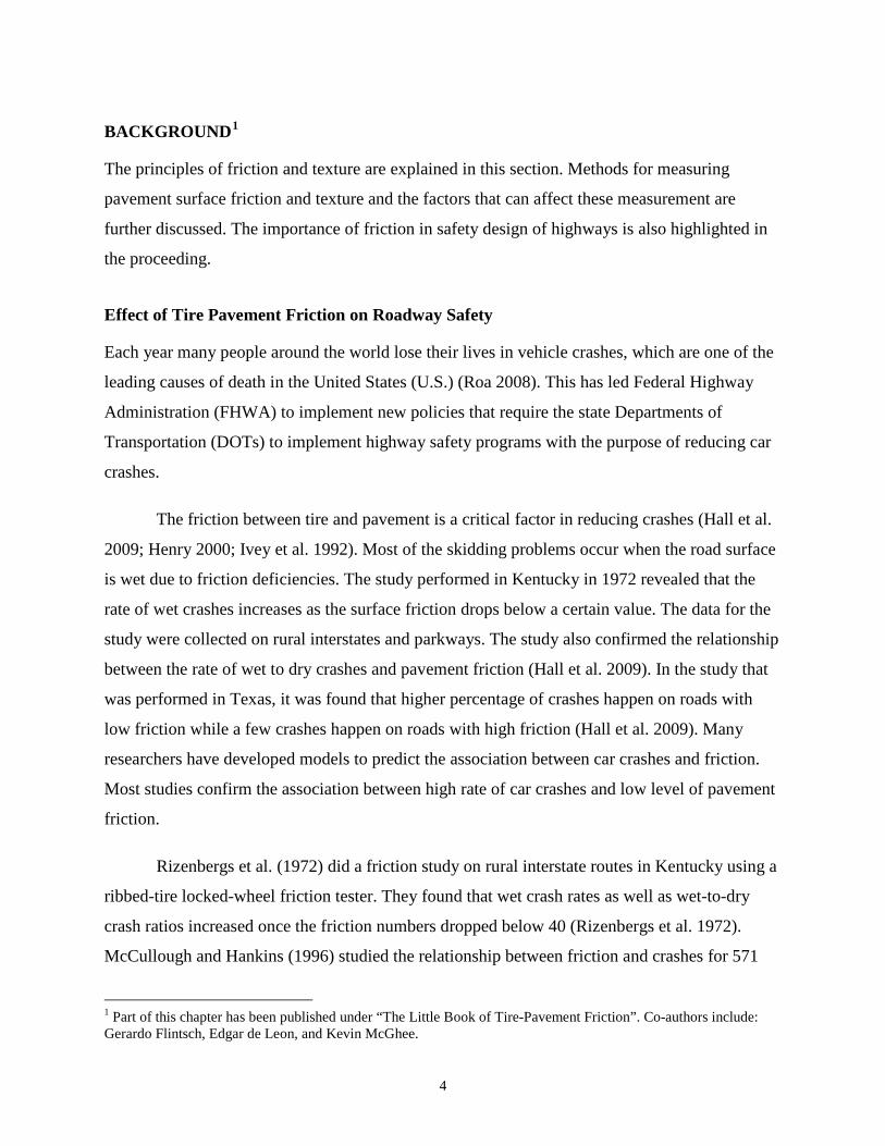
According to the AASHTO Guide for Pavement Friction; “pavement friction is the force that
resists the relative motion between a vehicle tire and a pavement surface” (FHWA 2010). The
friction force between tire and pavement is generally characterized by a dimensionless
coefficient known as coefficient of friction (µ), which is the ratio of tangential force at the
contact interface to the longitudinal force on the wheel. These forces are demonstrated in Figure
1.
Weight, Fw
Friction Force, F
Direction of motion
Rotation FwF
=m
Figure 1 Force body diagram for rotating wheel.
5
Tire-pavement friction is the result of the interaction between the tire and the pavement
not a property of the tire or the road surface individually. This interaction plays a critical role in
highway safety as it keeps the vehicles on the road by allowing drivers to make safe maneuvers.
It is also used in highway geometric design to determine the adequate minimum stopping
distance (Hall et al. 2009).
Pavement Surface Texture
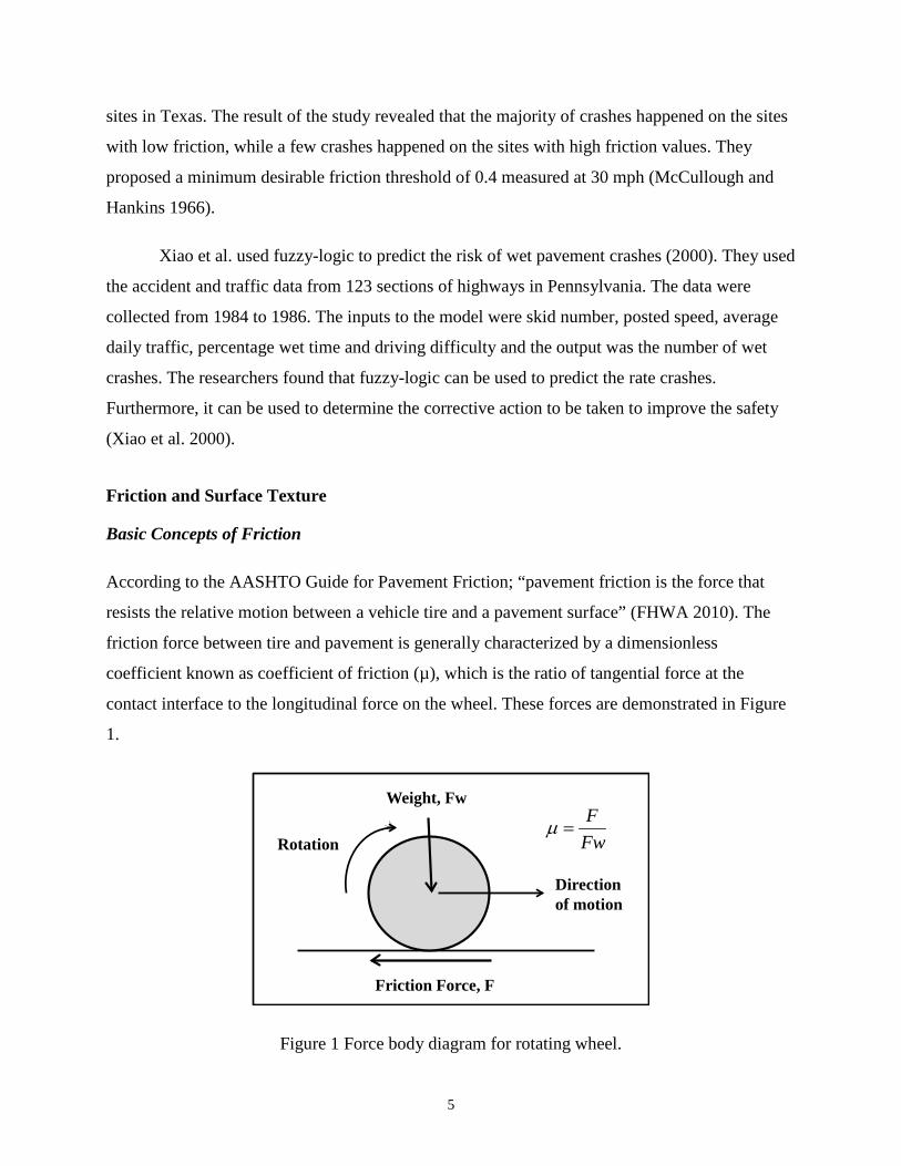
Pavement texture is defined by the AASHTO Guide for Pavement Friction as “the deviations of
the pavement surface from a true planar surface” (Hall et al. 2009). To classify the characteristics
of these deviations and their impact on pavement surface performance, the Permanent
International Association of Road Congress (PIARC) has defined a scale based on the
wavelength of the deviations (Figure 2).
0.00001 0.0001 0.001 0.01 0.1 1 10 100 ft10-6' 10-5' 10-4' 10-3' 10-2' 10-1' 100' 101' m
Int. Noise
Splash/Spray
Rolling Resistance
Tire Wear Tire/Vehicle Damage
Texture Wavelength
Microtexture Macrotexture Megatexture Roughness/Unevenness
Friction
Ext. Noise
Figure 2 Influence of texture wavelength on tire-pavement interaction (after Henry (2000)).
Tire-pavement friction is dominated by the texture of the surface, with different texture
components making different contributions. Of fundamental importance on both wet and dry
roads is the microtexture, that is, the fine-scale texture (below about 0.5 mm) on the surface of
the coarse aggregate in asphalt or the sand in cement concrete that interacts directly with the tire
6
rubber on a molecular scale and provide adhesion. This component of the texture is especially
important at low speeds but needs to be present at any speed.
On wet pavements, as speed increases skid resistance decreases and the extent to which
this occurs depends on the macrotexture, typically formed by shape and size of the aggregate
particles in the surface or by grooves cut into some surfaces. Generally, surfaces with greater
macrotexture have better friction at high speeds for the same low-speed friction (Roe and Sinhal
1998) but this is not always the case. Since all friction test methods can be insensitive to
macrotexture under specific circumstances, it is recommended that friction testing be
complemented by macro-texture measurement (ASTM E-1845). It has been found that at speeds
above 56 mph on wet pavements, macrotexture is responsible for a large portion of the friction,
regardless of the slip speed (Hall et al. 2009).
Components of Tire Pavement Friction
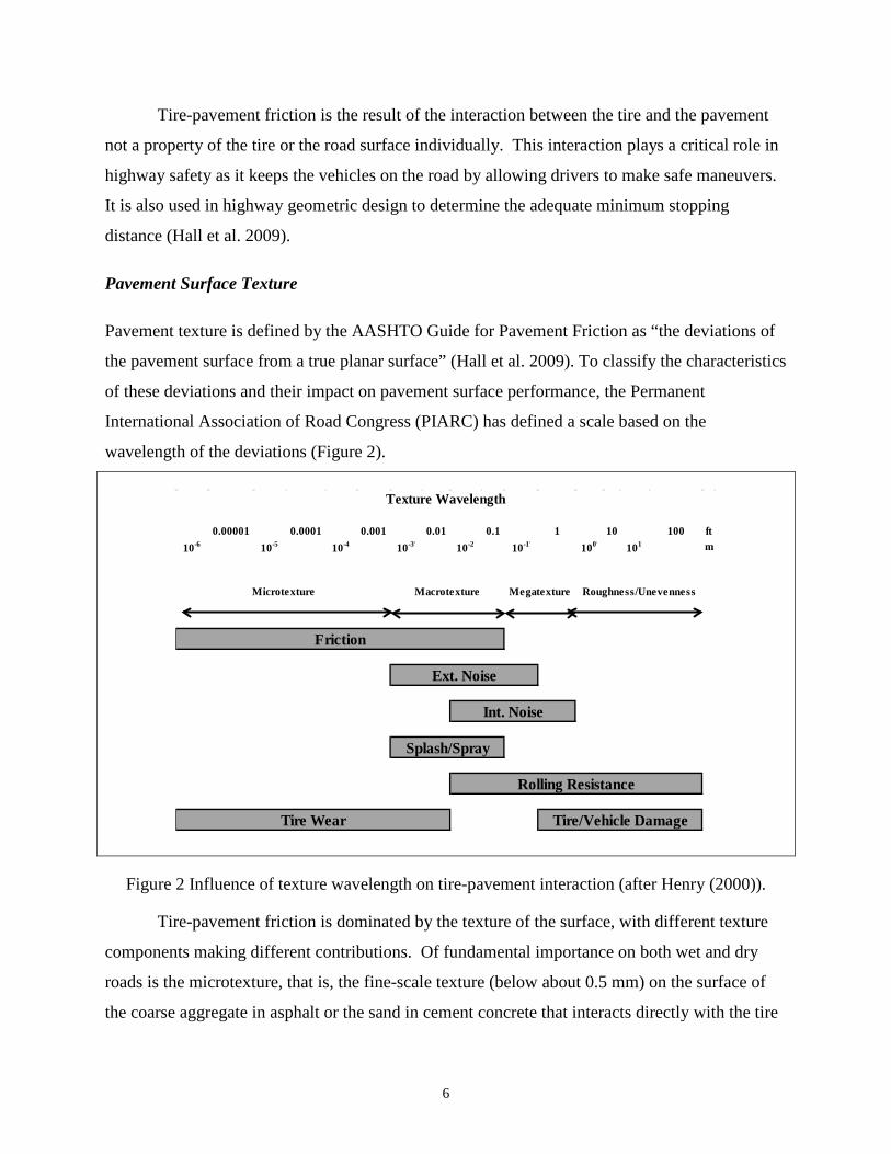
Tire pavement friction is the result of two main forces, adhesion and hysteresis. Adhesion is due
to the molecular bonding between the tire and the pavement surface while hysteresis is the result
of energy loss due to tire deformation. As the tire passes through pavement, surface texture
causes deformation in the tire rubber. This deformation is the potential energy stored in the tire.
As the tire relaxes part of this energy will be recovered and part of it will be dissipated in form of
heat. The generated heat (energy loss) is known as hysteresis. Both hysteresis and adhesion are
related to surface characteristics and tire properties (Hall et al. 2009). The key components of tire
pavement friction are illustrated in Figure 3.
Figure 3 Key components of tire pavement friction (after Hall et al. (2009)).
7

Braking, Accelerating, and Cornering
When a tire is free rolling in a straight line, the tire contact patch is instantaneously stationary
and there is little or no friction developed at the tire/road interface, although there may be some
interactions that contribute to rolling resistance. However, when a driver begins to execute a
maneuver that involves a change of speed or direction, forces develop at the interface in response
to acceleration, braking, or steering that cause a reaction between the tire and the road which
enables the vehicle to speed up, slow down, or track around a curve.
During braking, as the braking force increases, the reacting force increases until it
approaches a point at which the peak coefficient of friction available between the tire and the
road is exceeded (this normally occurs between 18 and 30 percent slip). At this point
(commonly known as “peak friction”), the tire continues to slow down relative to the vehicle
speed and to slip over the road surface, even though the wheel is still rotating. If the braking
force continues, the tire slips even more. Eventually complete locking of the wheel occurs, at
which time the wheel stops rotating and the tire contact patch skids over the road surface.
On a dry road surface, there is often little difference between peak and sliding friction
and relatively little effect of speed. However, on a wet road, peak friction is often lower than in
dry conditions, the sliding friction is typically lower than peak friction, and both usually (but not
always) decrease with increasing speed. The differences between wet and dry and peak and
sliding friction depend not only on vehicle speed and tire properties (including tread depth and
pattern), but also to a large extent on the characteristics of the road surface, particularly its state
of microtexture, the form and magnitude of the macrotexture, and the amount of water and other
contaminants on the pavement (the importance of which is discussed further below).
An analogous situation occurs during acceleration: although in normal circumstances the
tire contact patch remains instantaneously stationary, too great a demand for acceleration can
overcome the peak friction available and the wheel will start to slip, or in the extreme, to spin
with little or no vehicle acceleration (as on ice).
Similarly, in cornering, the side forces generated make the vehicle follow a curved path.
If the combination of forward speed and the effective radius of curvature (influenced by the
8
geometry of the road and steering angle) result in a demand for friction that exceeds what the
road can provide, the wheel may slip sideways. If the demand is high enough to overcome peak
friction, the wheel may slide sideways causing the vehicle to yaw. In this situation, a marked
difference between peak and sliding friction could lead to a rapid loss of control.
The situation is exacerbated when braking and cornering occur simultaneously, because
the available friction has to be shared between the two mechanisms. If the peak is exceeded, the
side-force goes down to near zero and the operator loses all control of steering. This is why anti-
lock braking systems (ABS) are important. They detect the onset of wheel slip and momentarily
release and then re-apply the brakes to make sure the peak friction is not exceeded and to reduce
the likelihood of side-slip occurring, thus helping the driver to maintain control. Similar ideas
are used in some modern vehicle control systems to reduce the risk of side-slip occurring under
simultaneous acceleration and cornering.
However, it is important to appreciate that while the instantaneous deceleration rates (and
inversely stopping distances) with ABS functioning may be greater than for a vehicle skidding
with locked wheels, there can be situations (particularly when the road is wet and the friction
level is low) when the average friction (including the times when the wheel is released as well as
those when it is slipping) will be less than in the locked-wheel condition.
Measuring tire-pavement friction
Since the friction depends on the interaction between the tire and the pavement, different
measurements are obtained for different testing conditions. This has led to the development of
different testing devices, which operate under different conditions. As the tire freely roles on the
pavement surface, longitudinal frictional forces generate at the tire and the pavement interface.
The relative speed between the tire circumference and the pavement surface (slip speed) is zero
(or very low) during free rolling (no braking) condition. Applying a constant brake to the tire
will increase the slip speed to the potential maximum equivalent of the vehicle speed. This
relationship can be mathematically expressed as follow (Hall et al. 2009):
)68.0( rVVVS P ××−=−= ω (1)
Where: S = Slip speed (mph)
9

V = Vehicle directional speed (mph) Vp = Average peripheral speed of tire (mph) ω = Angular velocity of the tire (radians/Second) r = Average radius of the tire (ft)
If the average peripheral speed of tire (Vp) is equal to the vehicle speed therefore the slip
speed (S) will be zero. During the fully locked wheel braking condition Vp is zero. This makes
the slip speed to be equal to vehicle speed. Most literature referred to locked wheel condition as
100 percent slip ratio and the free rolling condition as the zero slip ratio (fully locked condition).
The slip ratio can be mathematically expressed as follow (Hall et al. 2009):
100100 ×=×−
=VS
VVVSR P (2)
Where: SR = slip ratio.
When the vehicle steers around a curve or changes lanes another type of friction force
generates at the tire pavement interface. This type of friction is called lateral (side-force) friction
(Hall et al. 2009; Shahin 2005). The angle between test wheel and direction of travel is known as
“yaw angle”. The force-body diagram of a vehicle steering on a curve is shown in Figure 4.
According to the diagram the side force friction can be defined as (Shahin 2005).
surfaceroadandtirebetweenreactionverticalforcesidewaysSFC
⋅⋅⋅⋅⋅⋅⋅
= , (3)
Where: SFC = sideways friction coefficient.
The slip ratio of the test wheel is related to the yaw angle of the wheel and it can be
calculated as follow:
)(αSinAngleSlip =⋅ (4)
Where: α = Yaw angle.
10
Figure 4 Force-body diagram for a wheel traveling round a curve with constant speed (after Hall et al. (2009)).
Similar to slip speed, the slip ratio is zero during free rolling and it is maximum (100
percent) during fully locked condition. When a tire is free rolling in a straight line, the tire
contact patch is instantaneously stationary and there is little or no friction developed at the
tire/road interface, although there may be some interactions that contribute to rolling resistance.
However, when a driver begins to execute a maneuver that involves a change of speed or
direction, forces develop at the interface in response to acceleration, braking, or steering that
cause a reaction between the tire and the road which enables the vehicle to speed up, slow down,
or track around a curve.
Principles of Friction Measuring Equipment
Several different friction measuring devices have been developed over the years. They all rely
on the broad principle of sliding rubber over a road surface and measuring the reaction forces
developed in some way. There are essentially four general principles.
(i) Sliders, attached either to the foot of a pendulum arm or to a rotating head, which slow
down on contact with the road surface. The rate of deceleration is used to derive a value
representing the skid resistance of the road. A variant of this approach, still used by
police forces in some parts of the world, is to measure the reaction force when a sled
(with sliders representing car tires) is dragged over the road surface.
(ii) Sideway Force Coefficient (SFC) measurement uses an instrumented measuring wheel
set at an angle to the direction of travel of the vehicle. Although normally freely rotating
11
because it is set at an angle, the tire is made to slip over the road surface and the resulting
force along the wheel axle (the “side force”) is measured. The ratio of vertical and side
forces averaged over a defined measuring length provides the value that is recorded to
represent skid resistance. The wheel angle determines the slip ratio and the vehicle speed
determines the slip speed.
(iii) Longitudinal Friction Coefficient (LFC) measurement uses an instrumented measuring
wheel aligned with the direction of travel. A fixed gear or braking system forces the test
wheel to rotate slower than the forward speed. Consequently, the tire contact patch slips
over the road surface and a frictional force is developed that can be measured. Typically,
the ratio of vertical and drag forces is calculated (averaged over a fixed measuring length)
to provide a value representing the LFC that is recorded. Within this category there is a
wide range of slip ratios that may be used by individual devices. The slip ratio is usually
governed by the control system to a fixed proportion of the forward speed which, in turn,
determines the slip speed. Locked wheels (Figure 5) measure the longitudinal friction by
completely locking the brake of the measuring wheel, regardless of the test vehicle speed.
This simulates emergency braking without anti-lock brakes system (ABS). Locked
wheels can either use ribbed tire or smooth tire. Ribbed tires are knows to be less
sensitive to pavement macrotexture and water film depth than smooth tires. Figure 6
shows an example of a fixed-slip friction tester.
Figure 5 Locked-wheel friction tester.
12
Figure 6 GripTester.
(iv) Decelerometers are typically custom-made units mounted in a test vehicle, used to
measure the deceleration of a vehicle under emergency braking. Widely used by police
forces to assess road surface friction for collision investigations, and more recently in
experimental naturalistic driving studies, these devices are not suitable for road network
assessment or quality control purposes. They are further discussed later in this chapter.
Over the last several years, agencies around the world have started using Continuous
Friction Measuring Equipment (CFME) for highway friction management (mainly fixed-slip
technology). CFME has the advantage of operating under conditions similar to those of vehicles
equipped with ABS. They are designed to test the friction at a slip ratio between 10 to 30
percent, which is around the critical slip of most ABSs. Another advantage of these systems
over locked-wheels is that they continuously measure the friction across the entire stretch of a
road, providing greater detail about spatial variability of the tire-pavement frictional properties.
Furthermore, the locked-wheel testers and fixed slip devices like the GirpTester cannot measure
the lateral friction at curves as side force equipment does (Najafi et al. 2011).
To better understand the function of ABSs, the interaction between friction and the slip
ratio is illustrated in Figure 7. At zero slip (free rolling) there is no friction. Friction starts to
increase as the slip increases and reaches a peak friction value. Peak friction happens around
critical slip (typically between 10 to 30 percent). ABSs are designed to maintain the slip near the
13
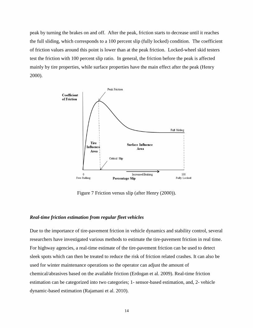
peak by turning the brakes on and off. After the peak, friction starts to decrease until it reaches
the full sliding, which corresponds to a 100 percent slip (fully locked) condition. The coefficient
of friction values around this point is lower than at the peak friction. Locked-wheel skid testers
test the friction with 100 percent slip ratio. In general, the friction before the peak is affected
mainly by tire properties, while surface properties have the main effect after the peak (Henry
2000).
Figure 7 Friction versus slip (after Henry (2000)).
Real-time friction estimation from regular fleet vehicles
Due to the importance of tire-pavement friction in vehicle dynamics and stability control, several
researchers have investigated various methods to estimate the tire-pavement friction in real time.
For highway agencies, a real-time estimate of the tire-pavement friction can be used to detect
sleek spots which can then be treated to reduce the risk of friction related crashes. It can also be
used for winter maintenance operations so the operator can adjust the amount of
chemical/abrasives based on the available friction (Erdogan et al. 2009). Real-time friction
estimation can be categorized into two categories; 1- sensor-based estimation, and, 2- vehicle
dynamic-based estimation (Rajamani et al. 2010).
14

Sensor-based Friction Estimation
Special sensors can be installed in the vehicle chassis or in the tire carcass to measure the friction
in real time. Varieties of sensors capable of measuring tire-pavement friction are documented in
the literature (Rajamani et al. 2010).
Acoustical sensors can be mounted in the car to record the sound made by the tire at the
interface and use that to estimate the friction at the tire-pavement interface (Rajamani et al.
2010). The correlation between tire noise levels and friction has been documented (Eichhorn and
Roth 1992). Correlation model between tire noise and friction can be used to estimate the friction
at the interface in real-time (Breuer et al. 1992; Eichhorn and Roth 1992).
Stresses and strains in the tire can also be used to estimate the tire-pavement friction
(Breuer, et al. 1992; Eichhorn and Roth 1992; Rajamani et al. 2010). Strain sensors can measure
the deformation in the tire at the contact patch in various directions and use that to estimate the
forces interfering at the tire-pavement interface. Using the magnitude and direction of these
forces will allow the estimation of friction at the contact patch possible (Rajamani et al. 2010).
Various types of optical sensors have also been implemented to estimate the road friction.
Optical sensors can detect surface type based on the ground reflection (Rajamani et al. 2010).
Several commercial systems are available that use the same concept to detect the snow and ice
on the road surface (SENSICE ; VAISALA). These systems are mostly used for winter
maintenance monitoring purposes. Some laser-based optical sensor cannot operate during wet
condition as the water on the pavement refracts the laser beam.
The main drawback of sensor-based estimation of tire-pavement friction is the cost
associated with acquiring the sensors. Sensors also have a limited service life which makes them
less desirable for frequent test applications. Frequent calibration requirements can also cause
user-time delays and it can increase the maintenance costs. Installing the sensors in the tire
carcass can also raise liability issues. Optical laser also have limited application during wet
weather condition. So for the above reasons this method was not implemented in this
dissertation.
15

Vehicle Dynamic Control-based Friction Estimation
In this approach tire-pavement friction is estimated based on the vehicle motion. This method
uses the measurements from the sensors already installed in the vehicle which gives it leverage
over sensor-based approach that requires additional sensors being installed in the car.
As the tire freely roles on the pavement surface, longitudinal frictional forces generate at
the tire and the pavement interface. The relative speed between the tire circumference and the
pavement surface (slip speed) is very low during free rolling (no braking) condition. Applying a
constant brake to the tire will increase the slip speed to the potential maximum equivalent of the
vehicle speed. The coefficient of friction can be determined based on the relationship between
normalized forces on the tire and the slip ratio (Rajamani et al. 2010). This relationship can be
explained by the “magic formula” tire model (Bakker et al. 1989; Pacejka and Bakker 1992). The
relationship between normalized tire forces versus slip ratio for various road surfaces with
different friction levels is presented in Figure 8.
Wet AsphaltHard SnowIce
Dry Concrete
0 0.05 0.1 0.15-0.05-0.1-0.15
0
0.40.2
0.60.81.0
-0.2-0.4-0.6-0.8-1.0
Longitudinal Slip
Nor
mal
ized
Lon
gitu
dina
l For
ce
Figure 8 Normalized longitudinal tire forces versus slip ratio (after Rajamani et al. (2010)).
16
For small slip ratios, the normalized tire forces are “proportional” to slip ratio (Rajamani
et al. 2010). The coefficient of friction can be determined based on the slope at the low slip
region – commonly known as “slip-slope” (Rajamani et al. 2010). The low slip/force data can be
measured from traction which usually happens during acceleration condition (Uchanski et al.
2003). Some references argue that tire properties influence the “shape” of the low slip region
versus the road surface properties (Henry 2000; Uchanski et al. 2003). It is cited that for slip
ratios greater than 0.005, the slip-slope method can reliably estimate the coefficient of friction
(Rajamani, Piyabongkarn et al. 2010). References (Dieckmann 1992; Germann et al. 1994;
Gustafsson 1997; Yi et al. 1999; Hwang and Song 2000) have used this method to estimate the
tire-pavement friction.
Another approach to finding the coefficient of friction is based upon the “saturated”
normal tire force (the peak force). As can be seen from Figure 2, normalized forces on the tire
“saturate” at high slip ratios and begin to decrease as the longitudinal slip increases. The
“saturated” normalized forces on the tire are proportional to the coefficient of friction and can be
used to estimate the coefficient of friction (Rajamani et al. 2010). Medium to high slip/force data
can be measured from braking (Uchanski et al. 2003).This method is demonstrated in Müller et
al. (2001) and Ray (1997).
Macrotexture Measuring Techniques
Macrotexture can be measured using both highway speed profilers and static methods. While
static devices can be used for project level measurements, the high speed devices are more
appropriate for network level data collection. There are two basic measurement techniques. The
oldest of these is the volumetric “patch” test in which a known volume of sand or glass beads (or
grease) is placed on the road surface and spread into a circular patch, filling the voids. The area
of the circle is measured and thus the average depth below the peaks in the surface is calculated
to give a value known as Mean Texture Depth (MTD).
In more recent years, laser displacement sensors, which measures along a narrow line
traversed by the laser (rather than across the area of a patch of sand or glass beads), have been
used to determine a surface profile from which a number of different parameters may be
calculated to represent the texture depth. Of these, root mean square (RMS) texture depth has
17

been used extensively both in research and as part of friction management in other countries.
However, the most widely used parameter internationally, and defined in the ASTM E-1845
standard, is the Mean Profile Depth (MPD), which also attempts to estimate the average depth
below the peaks in the surface. The standard device for measuring macrotexture is Circular
Track Meter (CTMeter) (ASTM E 2157). This static texture measuring device (Figure 9) has a
displacement sensor mounted on an arm at which rotates at a fixed elevation from the surface
collecting a high-resolution profile. The device is controlled by a computer that records the data
and reports the processed data as MPD and RMS. This device was found to have good
correlation with mean texture depth (MTD), which has been found highly correlated to speed
constant in the PIARC experiment described in the next section (Wambold et al. 1995).
Figure 9 Circular Track Meter (CTMeter).
Research is showing that although both are useful in some situations, an alternative to
RMS or MPD measures will likely be necessary to fully characterize road surface behavior.
What that index should be is not clear at the moment. A device that measures both, friction and
macrotexture, concurrently is needed to determine both low-speed and high-speed friction
performance (and their relative relevance in different situations) from a single measurement pass.
On dry pavement with good texture, the tire envelopes the texture and the depth of the
penetration in the footprint is a tire property; however, when wet, water can partially prevent the
penetration if the macrotexture is not deep enough. Tire tread and macrotexture sometimes are
18
not enough to allow the water to escape and thus causes the water to be present in the tire
pavement interface. MPD accounts for some of this, but not all and this needs to be taken into
consideration.
Operational Factors Affecting Friction Measurements
There are several operational factors that can affect the friction measurement. Better
understanding of these factors can help highway agencies to establish standard testing condition
and approaches for correcting measurement taken under other conditions.
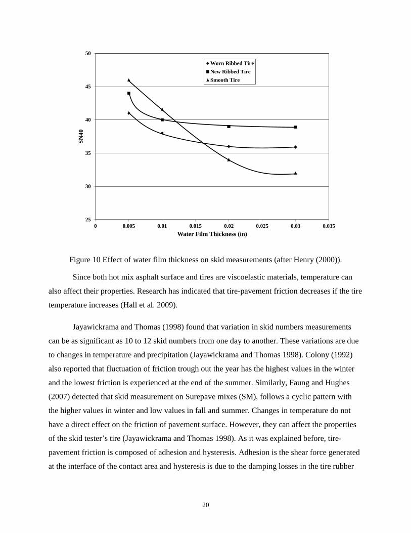
Water film thickness is one of the factors that have been proven to affect the friction
measurements. The water on the pavement surface decreases the tire-pavement contact area
which results in reduction in friction. This effect is known to be more noticeable at higher speeds
(>40 mph) compared to lower speeds (Hall et al. 2009). Worn tires are known to be more
sensitive to water film thickness. Pavement macrotexture and tires threads can provide channels
for water to escape through the tire-pavement contact area which result in increasing the traction
between tire and the pavement surface. The effect of water film thickness on locked wheel skid
trailer measurements is illustrated in Figure 10. The friction measurements (skid numbers) are
collected at 40 mph. Figure 10 suggests that smooth tires are more sensitive to the changes of
water film thickness. Due to the less sensitivity of ribbed tires to operational test conditions and
water film thickness some recommends them as the preferred choice for friction measurements
(Henry 2000). However, since ribbed tires are less sensitive to the pavement macrotecxture is it
recommended that their measurements be accompanied by macrotexture measurements. Recent
studies have also confirmed the sensitivity of Continuous Friction Measuring Equipment
(CFME) to water film thickness and other operational test conditions (Najafi et al. 2012).
19
25
30
35
40
45
50
0 0.005 0.01 0.015 0.02 0.025 0.03 0.035
SN40
Water Film Thickness (in)
Worn Ribbed TireNew Ribbed TireSmooth Tire
Figure 10 Effect of water film thickness on skid measurements (after Henry (2000)).
Since both hot mix asphalt surface and tires are viscoelastic materials, temperature can
also affect their properties. Research has indicated that tire-pavement friction decreases if the tire
temperature increases (Hall et al. 2009).
Jayawickrama and Thomas (1998) found that variation in skid numbers measurements
can be as significant as 10 to 12 skid numbers from one day to another. These variations are due
to changes in temperature and precipitation (Jayawickrama and Thomas 1998). Colony (1992)
also reported that fluctuation of friction trough out the year has the highest values in the winter
and the lowest friction is experienced at the end of the summer. Similarly, Faung and Hughes
(2007) detected that skid measurement on Surepave mixes (SM), follows a cyclic pattern with
the higher values in winter and low values in fall and summer. Changes in temperature do not
have a direct effect on the friction of pavement surface. However, they can affect the properties
of the skid tester’s tire (Jayawickrama and Thomas 1998). As it was explained before, tire-
pavement friction is composed of adhesion and hysteresis. Adhesion is the shear force generated
at the interface of the contact area and hysteresis is due to the damping losses in the tire rubber
20
(Li et al. 2004). Higher temperature makes the tire more flexible. This reduces the energy loss of
the tire (hysteresis) and decreases the measured skid number. Nevertheless there is no proof
available for this mechanism in the literature. While some studies stated that the effect of
temperature is a very insignificant; many others indicate that temperature is a significant factor
(Jayawickrama and Thomas 1998). Bazlamit and Reza (2005) indicated that regardless of the
surface texture, increasing the temperature decreases the hysteresis component of surface friction
while for adhesion component, surface texture affects this behavior (Bazlamit and Reza 2005).
Since hysteresis accounts for greater part of total friction, the combined friction of the surface
decreases with increasing temperature (Bazlamit and Reza 2005).
Hill and Henry (1982) proposed a model that predicts the seasonal variation in the skid
number intercept (SN0). The analysis was based on the data collected on test sites in
Pennsylvania from 1978 to 1980.
Pavement Friction Management
Pavement friction management includes both engineering practices to provide a pavement
surface with adequate and durable friction and also periodic data collection and analysis to
ensure the effectiveness of these practices.
If the reason that the road is slippery is due to some external factor, such as ice on the
surface or a local oil spillage, there is little that the road engineer can do, apart from taking
measures to prevent ice from forming or having procedures in place to clean up spills. If,
however, the road has inherently poor skid resistance because of the materials of which it is
made and how those materials have reacted to the passage of traffic over time, then it can be said
that the road may contribute to crashes and road engineers should be able to detect such
situations and take appropriate action. Inadequate cross slope and/or grade can also contribute to
crashes by contributing to flooding the road.
Friction demand
Friction demand is the level of friction needed to safely perform braking, steering, and
acceleration maneuvers. Factors such as traffic volume, geometrics (curves, grades, sight
distance, etc.), potential for conflicting vehicle movements, and intersections should be
21
considered for determining friction demand. Curves and intersections also tend to lose friction at
a faster rate than other roadway locations and thus justify a higher friction demand. Highway
agencies can establish Investigatory Level (desirable) and Intervention Level (minimum) values
for pavement friction and texture in accordance with AASHTO Guide for Pavement Friction.
AASHTO “Guide for Pavement Friction” has defined three methods to establish two
distinctive friction threshold levels – investigatory and intervention. The sites with the friction
values below investigatory level will be selected for detailed investigation to determine if there is
a need for posting warning signs. The sites with friction values below intervention level are
typically selected for corrective action such as resurfacing or other programmatic maintenance
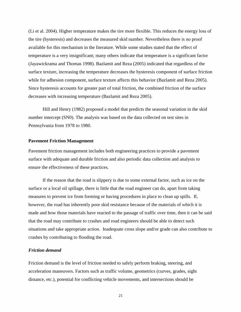
treatment. The first method uses the friction deterioration curve by plotting friction loss versus
pavement age. The friction value at which significant loss rapidly begins is selected as
investigatory level as shown in Figure 17. An intervention level can be defined at a fixed
percentage below the investigatory level (Hall et al. 2009).
Figure 11 Friction deterioration curve (after Hall et al. (2009)).
The second method uses both friction deterioration curve as well as the historical crash
data. The investigatory level is set where there is a significant drop in friction level and the
intervention method is set where there is significant increase in crashes (Figure 18) (Hall et al.
2009).
22

Figure 12 Investigatory and Intervention friction level based on friction deterioration and crash rate (after Hall et al. (2009)).
Finally, the third method uses the friction distribution and crash rate for each roadway
category to determine the investigatory and intervention level of friction. The histogram of
pavement friction and wet-to-dry crash ratio is plotted first (Figure 19). The mean and standard
deviation of friction distribution are then calculated. The investigatory level is set as the mean
friction minus “X” (e.g. 1.5 or 2.0) standard deviation and it is adjusted to where wet-to-dry
crashes begin to increase considerably. The intervention level is set as the mean friction minus
“Y” (e.g. 2.5 or 3.0) standard deviation and it is adjusted to minimum satisfactory wet-to-dry
crash rate or by the point where enough funding is available to address the friction deficiencies
(Hall et al. 2009). This method is more practical than other two approaches since agency can
adjust the intervention friction level based on available funding.
23
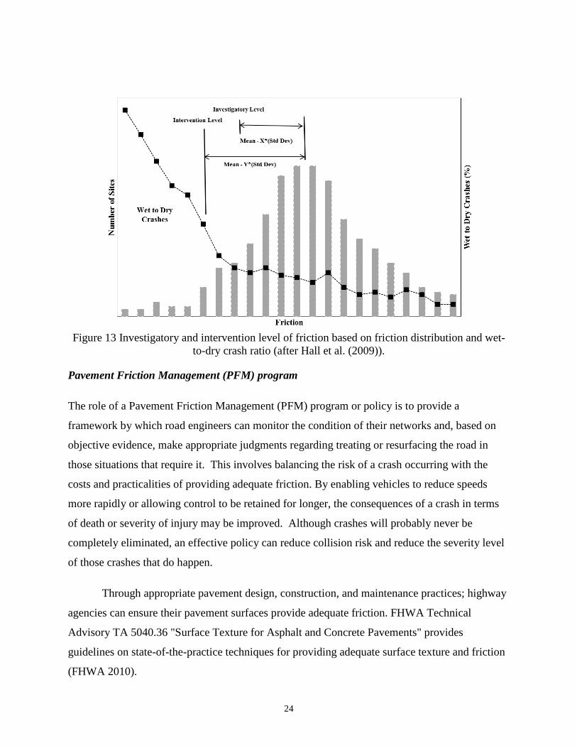
Figure 13 Investigatory and intervention level of friction based on friction distribution and wet-to-dry crash ratio (after Hall et al. (2009)).
Pavement Friction Management (PFM) program
The role of a Pavement Friction Management (PFM) program or policy is to provide a
framework by which road engineers can monitor the condition of their networks and, based on
objective evidence, make appropriate judgments regarding treating or resurfacing the road in
those situations that require it. This involves balancing the risk of a crash occurring with the
costs and practicalities of providing adequate friction. By enabling vehicles to reduce speeds
more rapidly or allowing control to be retained for longer, the consequences of a crash in terms
of death or severity of injury may be improved. Although crashes will probably never be
completely eliminated, an effective policy can reduce collision risk and reduce the severity level
of those crashes that do happen.
Through appropriate pavement design, construction, and maintenance practices; highway
agencies can ensure their pavement surfaces provide adequate friction. FHWA Technical
Advisory TA 5040.36 "Surface Texture for Asphalt and Concrete Pavements" provides
guidelines on state-of-the-practice techniques for providing adequate surface texture and friction
(FHWA 2010).
24

Locations with high rate of wet-weather crashes need to be identified and investigated for the
purposes of minimizing friction-related crash rates. The procedure is commonly done by
calculating the ratio between wet weather crashes and total crashes (wet + dry) and then
following one of the subsequent approaches (FHWA 2010):
• Agencies may use a specific value for the wet crash ratio above which a location will be
identified as an elevated wet-weather crash location. Depending on geographical and
climate circumstances this ratio can vary between 0.25 and 0.5.
• Agencies may compare the wet crash ratio with the average ratio for that functional class
of highway in that area. If the computed ratio is above the average by a specified
percentage that location is identified as an elevated wet-weather crash location.
• A minimum number of wet-weather or total crashes within a segment is another criterion
that some agencies use in order for a segment to be identified as an elevated wet-
weather crash location.
Frequency of friction testing
The facilities with the highest traffic volumes, the highest likelihood of changes in friction over
time, and the highest friction demand justify the most frequent monitoring of friction. A risk-
based approach can be implemented to determine the frequency of the friction test for roadway
networks. Facilities with higher friction demand require more frequent friction monitoring. Many
agencies monitor the friction of their important roadway network on an annual basis. While a 2
to 3 year cycle may be appropriate for the part of network with lower-risk (FHWA 2010).
Achieving and Maintaining Adequate Tire-pavement Friction
Designing for Friction
Pavement friction design involves utilizing proper materials and construction techniques to
achieve high level of microtexture and microtexture in the pavement surface. Type of the
aggregates used in the surface mix directly affects the microtexture while gradation and size of
aggregates governs the macrotexture properties of pavement surface. In asphalt mixtures, large
25

aggregates govern the frictional properties of the surface while for concrete mixes, fine
aggregates control the frictional properties (Hall et al. 2009).
The wear characteristics of aggregates are also important in maintaining proper friction
level. Aggregates mineralogy and hardiness directly affect the durability and polish ability of the
aggregates. It is generally better to have aggregates with different size and wear characteristics in
the mix so they can constantly renew the surface (Hall et al. 2009).
Restoring Friction
There are several methods that can be used to restore the frictional properties of old pavements.
Diamond grooving is a technique that is used in order to improve the frictional properties of the
pavement surfaces (Martinez 1977). This method is mostly used for concrete pavements. The
method uses diamond infused steel cutting blades for grinding and grooving concrete pavement.
For grinding, the blades are spaced close together so that they can cut the pavement’s unevenness
(megatexture) and leave a rough pavement surface (high microtexture). For grinding, the blades
are further spaced out so they create channels on the pavement surface (high macrotexture).
Diamond grooving is mainly used for new concrete pavement to texture the pavement which
increases the friction by improving water drainage (Wulf et al. 2008). More discussion on the
effect of diamond grinding and grooving on restoring pavement friction is provided in the
chapter 5 of the dissertation.
Using High Friction Surfaces (HFS) and epoxy overlays is another option to increase the
surface friction. This method can increase the surface friction without jeopardizing other surface
characteristics including noise and durability. HFS treatments utilize a durable aggregate and
some type of resin (binder) to hold the aggregate particles together and glued to the road surface.
There are several types of HFS commercially available in the market including: Cargill,
Tyregrip, Italgrip, Crafco, and Flexogrid (Roa 2008).
SUMMARY
The principles of friction and texture and the factors affecting these measurements were
discussed in this chapter. The importance of friction in safety was also highlighted. Most of the
26

past literature is focused on the effect of friction on wet crashes. Chapter two of the dissertation
investigates the effect of friction on dry crashes as well.
Several methods for defining minimum acceptable friction threshold were demonstrated.
Most of these methods require historical friction data which is not readily available. Chapter
three and four introduce an alternative method based on soft-computing to define an allowable
friction threshold.
REFERENCES
Adewole, A. (2008). "Deliverable 02: Report on Dissemination Strategy, Tyre and Road Surface
Optimisation for Skid Resistance and Further Effects (TYROSAFE), Forum of European
National Highway Research Laboratories (FEHRL)."
Arndt, M., E. Ding, et al. (2004). “Identification of cornering stiffness during lane change
maneuvers”. Control Applications, 2004. Proceedings of the 2004 IEEE International
Conference on, IEEE.
Baffet, G., A. Charara, et al. (2006). “Sideslip angle, lateral tire force and road friction
estimation in simulations and experiments”. Computer Aided Control System Design, 2006
IEEE International Conference on Control Applications, 2006 IEEE International Symposium on
Intelligent Control, 2006 IEEE, IEEE.
Bakker, E., H. B. Pacejka, et al. (1989). "A new tire model with an application in vehicle
dynamics studies." SAE paper 890087.
Bazlamit, S., and Reza, F. (2005). "Changes in Asphalt Friction Components and Adjustment
Number for Temperature." The Journal of Transportation Engineering, ASCE 2005:131-470.
Breuer, B., U. Eichhorn, et al. (1992). “Measurement of tyre/road-friction ahead of the car and
inside the tyre”. International Symposium on Advanced Vehicle Control, 1992, Yokohama,
Japan.
Colony, D. (1992). "Influence of traffic, surface age and environment on skid number." Ohio
Department of Transportation Project Number 14460 Final Report, Columbus, Ohio.
27
Dieckmann, T. (1992). "Assessment of Road Grip byWay of Measured Wheel Variables."
Proceedings of FISITA ’92 Congress, London, GB, 2:75–81, June 7–11. ‘‘Safety the Vehicle and
the Road.’’.
Eichhorn, U. and J. Roth (1992). “Prediction and monitoring of tyre/road friction”. XXIV
FISITA Congress, 7-11 June 1992, London. Helt at the Automotive Technology Servicing
Society. Technical Papers. “Safety, The vehicle and the road”. Volume 2, (IMECHE NO
C389/321 AND FISITA NO 925226).
Erdogan, G., L. Alexander, et al. (2009). "Friction coefficient measurement for autonomous
winter road maintenance." Vehicle System Dynamics 47(4): 497-512.
Faung, H., and Hughes, W. (2007). "Friction Monitoring of SuperPave Mixes in Virginia."
Virginia Highway & Transportation Research Council: 8-9.
FHWA (2010). "Technical Advisory T5040.38, Pavement Friction Management."
Flintsch, G. W., K. K. McGhee, et al. (2012). "The Little Book of Tire Pavement Friction."
Germann, S., M. Wurtenberger, et al. (1994). “Monitoring of the friction coefficient between tyre
and road surface”. Control Applications, 1994., Proceedings of the Third IEEE Conference on,
IEEE.
Gustafsson, F. (1997). "Slip-based tire-road friction estimation." Automatica 33(6): 1087-1099.
Gustafsson, F. (1998). "Monitoring tire-road friction using the wheel slip." Control Systems,
IEEE 18(4): 42-49.
Gustafsson, F. (2000). “Adaptive filtering and change detection”, Wiley New York.
Hahn, J.-O., R. Rajamani, et al. (2002). "GPS-based real-time identification of tire-road friction
coefficient." Control Systems Technology, IEEE Transactions on 10(3): 331-343.
Hall, J. W., K. L. Smith, et al. (2009). “Guide for pavement friction”, National Cooperative
Highway Research Program, Transportation Research Board of the National Academies.
28

Henry, J. J. (2000). "Evaluation of Pavement Friction Characteristics: A Synthesis of Highway
Practice, NCHRP Synthesis 291, Transportation Research Board, National Research Council,
Washington, D.C.".
Hosking, J. (1986). "Relationship between skidding resistance and accident frequency estimates
based on seasonal variation." TRRL Research Report 76, Transport Research Laboratory,
Crowthorne, UK.
Hwang, W. and B.-S. Song (2000). “Road condition monitoring system using tire-road friction
estimation”. Proceedings of AVEC 2000 5th International Symposium of Advanced Vehicle
Control.
Ivey, D. L., Griffin III, L. I., Lock, J. R., and Bullard, D. L. (1992). "Texas Skid Initiated
Accident Reduction Program."
Jayawickrama, P., and Thomas, B. (1998). "Correction of Field Skid Measurements for Seasonal
Variations in Texas." Transportation Research Board 1639:147-152.
Li, S., Noureldin, S., and Zhu, K. (2004). "Upgrading the INDOT Pavement Friction Testing
Program." Joint Transportation Research Program, Perdue Libraries: 6-9.
Martinez, J. (1977). "Effects of pavement grooving on friction, braking, and vehicle control."
McCullough, B.V., and Hankins, K.D., 1966. “Skid resistance guidelines for surface
improvements on Texas highways”. Highway Research Record, 131, 204–217.
Müller, S., M. Uchanski, et al. (2001). “Slip-based tire-road friction estimation during braking”.
Proceeding of IMECE’01 (2001 asme International Engineering Congress and Exposition).
Najafi, S., Flintsch, G. W., and McGhee, K. K. (2012). "Assessment of operational
characteristics of continuous friction measuring equipment (CFME)."
Najafi, S., Flintsch, G. W., de Leon Izeppi, E. D., McGhee, K. K., and Katicha, S.
"Implementation of Cross-Correlation to Compare Continuous Friction Measuring Equipment
(CFME)."
29
NHTSA, N. H. T. S. A. "2010 Motor Vehicle Crashes: Overview." [online], available at:
http://www-nrd.nhtsa.dot.gov/Pubs/811552.pdf. accessed on March 20, 2013.
Pacejka, H. B. and E. Bakker (1992). "The magic formula tyre model." Vehicle System
Dynamics 21(S1): 1-18.
Rajamani, R., N. Piyabongkarn, et al. (2010). "Tire-road friction-coefficient estimation." Control
Systems, IEEE 30(4): 54-69.
Ray, L. R. (1997). "Nonlinear tire force estimation and road friction identification: simulation
and experiments." Automatica 33(10): 1819-1833.
Rizenbergs, R.L., Burchett, J.L., and Napier, C.T., 1972. “Skid resistance of pavements, Part II”.
Lexington, Kentucky: Kentucky Department of Highways, Report No. KYHPR-64-24.
Roa, J. A. (2008). "Evaluation of International Friction Index and High Friction Surfaces."
Virginia Polytechnic Institute and State University.
Roe, P. G., and Sinhal, R. (1998). "The Polished Stone Value of aggregates and in-service
skidding resistance." TRL Report 322, TRL, Crowthorne, UK.
Sastry, S. and M. Bodson (2011). “Adaptive control: stability, convergence and robustness”,
Courier Dover Publications.
SENSICE [online], available at: http://www.sensice.com/. accessed on March 20, 2013.
Shahin, M. Y. (2005). “Pavement management for airports, roads, and parking lots”, Springer
Verlag.
Sierra, C., E. Tseng, et al. (2006). "Cornering stiffness estimation based on vehicle lateral
dynamics." Vehicle System Dynamics 44(sup1): 24-38.
TTI, T. T. I. (Accessed on June 13, 2012). [online] available at:
http://tti.tamu.edu/group/crashtesting/research-areas/#area4.
30
Uchanski, M., K. Hedrick, et al. (2003). "Estimation of the maximum tire-road friction
coefficient." Journal of dynamic systems, measurement, and control 125(4): 607-617.
VAISALA [online], available at: http://www.vaisala.com. accessed on March 20, 2013.
Viner, H. E., Parry, A. R., and Sinhal, R. (2005). "Linking road traffic accidents with skid
resistance – recent UK developments, International Conference on Surface Friction of Roads and
Runways, Christchurch, New Zealand."
Wambold, J., Antle, C., Henry, J., and Rado, Z. (1995). "PIARC (Permanent International
Association of Road Congress) Report." International PIARC Experiment to Compare and
Harmonize Texture and Skid Resistance Measurement, C-1 PIARC Technical Committee on
Surface Characteristics, France.
Wulf, T., Dare, T., and Bernhard, R. (2008). "The effect of grinding and grooving on the noise
generation of Portland Cement Concrete pavement." Journal of the Acoustical Society of
America, 123(5), 3390.
Xiao, J., B. T. Kulakowski, and M. El-Gindy (2000). “Prediction of Risk of Wet-Pavement
Accidents: Fuzzy Logic Model”, Transportation Research Record 1717, Transportation Research
Board, Washington, D.C.
Yi, K., K. Hedrick, et al. (1999). "Estimation of tire-road friction using observer based
identifiers." Vehicle System Dynamics 31(4): 233-261.
31
CHAPTER 2 - LINKING ROADWAY CRASHES AND TIRE–PAVEMENT
FRICTION: A CASE STUDY2
ABSTRACT
Tire-pavement friction is a factor that can affect the rate of car crashes. Several studies have
suggested that reduced friction during wet weather conditions, due to water on the pavement
surface reducing the contact area between the tire and the pavement, increases vehicle crashes.
This study evaluates the effect of friction on both wet- and dry-condition crashes. The data for
the study were provided by the New Jersey Department of Transportation. Regression analysis
was performed to verify the effect of friction on the rate of wet- and dry-condition car crashes for
various types of urban roads. It was found that friction is not only associated with the rate of
wet-condition car crashes, but it also impacts the rate of dry-condition car crashes. The analysis
also suggested that the developed regression models could be used to define the friction demand
for different road categories.
2 This manuscript has been published in the International Journal of Pavement Engineering (IJPE). DOI:10.1080/10298436.2015.1039005. Co-authors include: Gerardo Flintsch, and Alejandra Medina.
32
INTRODUCTION
Each year many people around the world lose their lives in vehicle crashes, which are one of the
leading causes of death in the United States. According to a National Transportation Safety
(N.T.S.) report, car crashes injure or disable more than 3.2 million people each year in the United
States. Every twelve minutes, one person dies in a motor vehicle crash in the United States.
These accidents have a great influence on economics and health services (Roa 2013). This has
led the Federal Highway Administration (FHWA) to implement new policies that require the
state Departments of Transportation (DOTs) to implement highway safety programs with the
purpose of reducing car crashes. Several factors, including the driver, the vehicle, the
environment, and the roadway infrastructure, can influence the rate of car crashes. Of all these
factors, transportation engineers can control only the roadway design factor, which includes road
geometry, grade, and surface friction (Flintsch et al. 2012). Highway agencies generally monitor
pavement friction as part of their asset management efforts due to its importance in reducing car
crashes.
The relationship between friction and car crashes has been well studied by several
researchers. Kuttesch developed a model to quantify the effect of friction on wet-weather crashes
for the state of Virginia (Kuttesch 2013). Larson et al. studied the effect of friction on wet-
condition crashes for the Ohio Department of Transportation (ODOT). The result of the study
was a comprehensive list of recommendations for ODOT to improve their roadway network
safety (Larson et al. 2013). Schram performed a correlation analysis between the ratio of wet-
condition to dry-condition crashes and friction using Iowa DOT data. He further used the model
to define the minimum desirable friction level and a specification for aggregate frictional
qualities (Schram 2011). Davies et al. studied the effect of friction and texture depth on crash
risk for New Zealand’s state highway network. They also incorporated the effect of geometry
(e.g., curvature, gradient), surface condition (e.g., roughness, rut depth), and roadway
characteristics (e.g., region, urban versus rural, traffic flow) into the study (Davies et al. 2005).
Viner et al. investigated the link between friction and accidents for the United Kingdom (U.K.)
highway network. They found that although skid resistance is an important factor affecting the
rate of accidents, the “nature” of this effect is “site specific” (Viner et al. 2004). They later
developed a new investigatory friction level for various site categories (Viner et al. 2005).
33

BACKGROUND
Friction is an important performance parameter of the road surface. It is defined as the force that
provides resistance to slipping when the tires are prevented from rolling (Shahin 2005). The
friction between tire and pavement is a critical factor in reducing crashes (Henry 2000, Ivey
1992). Most skidding problems occur when the road surface has friction deficiencies due to
wetness (Flintsch et al. 2012). According to some sources, one third of all wet-condition crashes
are related to surface characteristics of roadways (Fwa 2005). Traditionally, it has been found
that pavement friction is high during dry conditions. Data collected with a Sideway-force
Coefficient Routine Investigation Machine (SCRIM) device has proven that dry friction is very
similar for various surfaces (Fwa 2005). Once the pavement gets wet, surface friction drops
significantly. Pavement surface friction gradually drops as the water film thickness increases;
however, the changes in pavement surface friction are not substantial (Fwa 2005). Several
studies have quantified the effect of water film thickness on surface friction (Najafi et al. 2013,
Kulakowski et al. 1990, Rose et al. 1997).
Several factors can affect pavement friction. According to Hall et al. (2009) these factors
can be classified into four groups: (1) pavement surface characteristics (i.e., microtexture,
macrotexture, material properties, and temperature), (2) vehicle operating parameters (i.e., slip
speed, driving maneuver), (3) tire properties (i.e., footprint, tread design, inflation pressure,
rubber composition, and temperature), and (4) environment (i.e., climate, temperature, water,
snow and ice, and contamination) (Hall et al. 2009). Seasonal variations can have a significant
effect on pavement friction (Fwa 2005). This effect can be explained by changes in temperate
and precipitation (Jayawickrama 1998). Overalls friction is lower in summer months compared
to other times of the year. This is mainly due to accumulation of polished particles from
pavement or contamination from vehicles (Flintsch et al. 2012). Since both hot-mix asphalt
surface and tires are viscoelastic materials, temperature can affect their properties. Several
researchers have studied the effect of temperature on pavement friction measurements (Bianchini
et al. 2011, Bazlamit et al. 2005). Although several attempts have been made to quantify the
effect of seasonal variation on friction measurement (Jayawickrama 1998, Hill et al. 1981,
Flintsch et al. 2009, FHWA 2010), there is no practical model currently available for this
purpose.
34
Friction measurements are typically collected as part of the state’s wet accident reduction
program (WARP) on areas with a high rate of car crashes. This means that data collection is
mostly being done at the project level on specific areas. Statistics show that 55.4% of agencies
collect friction measurements at the project level. Only 33.9% of agencies collect network-level
friction data (Flintsch et al. 2009). To be able to collect network-level friction data, agencies
need to implement equipment with high daily output. In the United States, locked-wheel trailers
are the most predominant friction tester used by state DOTs. They measure the steady state
friction—also called Skid Number (SN)—on a fully locked wheel at a certain speed 64 kph (40
mph) based on the ASTM standard). The locked wheels use two types of test tires; Smooth
(ASTM E-524) and Ribbed (ASTM E-501). Figure 14 shows a locked-wheel skid trailer. The
SCRIM is the most commonly used friction tester in Europe. SCRIM devices can measure
friction continuously. The device has a bigger water tank compared to locked-wheel trailers, so it
can test a longer length of roadway network, on average, 200 km (125 miles) of roadway every
day (Fwa 2005).
Figure 14 Locked-wheel trailer.
Friction data can be used in developing Pavement Friction Management (PFM) programs.
PFM includes engineering practices and periodic data collection to ensure an adequate friction
level for the riding surface. This can be achieved by using appropriate pavement design,
35
construction, and maintenance techniques. Guidelines and techniques for providing adequate
surface texture and friction levels can be found in FHWA Technical Advisory TA 5040.36,
“Surface Texture for Asphalt and Concrete Pavements” (FHWA 2013). Locations with high rates
of wet-condition crashes need to be identified and further investigated. This can be done by
computing the ratio between wet-condition crashes and total crashes (wet- and dry-condition)
and then using one of the following procedures (FHWA 2013):
• Set a specific threshold for the wet-condition crash ratio, above which a location will be
identified as an elevated wet-condition crash location. This ratio can vary between 0.25
and 0.5, depending on geographical and climate conditions.
• Compare the wet-condition crash ratio with the average crash ratio for a specific highway
functional class in that area. The location will be identified as an elevated wet-condition
crash location if the computed ratio is above the average by a specified percentage.
• Set the threshold at the minimum of the total number of crashes within a segment.
The American Association of State Highway and Transportation Officials (AASHTO) Guide
for Pavement Friction Management outlines several methods for highway agencies to establish
Investigatory Level (desirable) and Intervention Level (minimum) thresholds for pavement
friction and texture (Hall et al. 2009). Most of these methods require historical data for pavement
friction, which are not readily available for most states.
OBJECTIVE
This paper investigates the effect of friction on the rate of fatal and injury-causing car crashes on
urban roads. The effect of friction on the rate of both wet-condition and dry-condition crashes is
evaluated. The data for this study were provided by New Jersey Department of Transportation.
DATA COLLECTION
The friction database includes the network-level friction measurements collected by a ribbed-tire,
locked-wheel skid trailer. The friction database also includes traffic (Annual Average Daily
Traffic (AADT)), speed limit, road functional class (Urban Interstate, Urban Principle Arterial,
etc.), and the location (route name and the milepost) of the collected data.
36
The crash database includes the location information of the crashes (route and milepost),
type of accident (fatal, injury-causing, etc.), road surface condition at the time of accident (wet,
dry, etc.), and the date of the accident. The analysis of this project considered only the crashes
that had at least one injury or fatality. For practicality, only the data for one year (2007) were
analyzed.
DATA ANALYSIS
The first step for analyzing the data was to match up the friction measurements with
corresponding crash location. This was done by comparing the route and milepost information. If
the difference between the milepost of the crash location and the friction measurement that were
on the same route was less than 0.1 miles they were matched. The summary of the crashes that
were successfully matched with friction locations are provided in Table 1. Since urban collector,
urban local, and all rural roads had very few matched locations compared to other types of roads,
they were not included in further analysis.
Table 1 Fatal and Injury-Causing Accident Counts
# of sites with accidents
Functional Class Surface
Condition Dry Wet
Urban Principal Arterial 20308 5010 Urban Interstate 3963 1251 Urban Minor Arterial 2979 714 Urban Freeway Expressway 2409 665 Urban Collector 20 11 Urban Local 12 4 Rural Principal Arterial 758 166 Rural Interstate 510 170 Rural Major Collector 687 158
Friction measurements were divided into intervals (bins) with increments of two friction
units (20: SN below 20, 22: 20 < SN ≤ 22, etc.) and the numbers of crashes for each friction
37
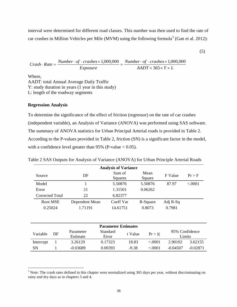
interval were determined for different road classes. This number was then used to find the rate of
car crashes in Million Vehicles per Mile (MVM) using the following formula3 (Gan et al. 2012):
(5)
LYAADT
crashesofNumberExposure
crashesofNumberRateCrash×××
×⋅⋅=
×⋅⋅=⋅
365000,000,1000,000,1
Where, AADT: total Annual Average Daily Traffic Y: study duration in years (1 year in this study) L: length of the roadway segments
Regression Analysis
To determine the significance of the effect of friction (regressor) on the rate of car crashes
(independent variable), an Analysis of Variance (ANOVA) was performed using SAS software.
The summary of ANOVA statistics for Urban Principal Arterial roads is provided in Table 2.
According to the P-values provided in Table 2, friction (SN) is a significant factor in the model,
with a confidence level greater than 95% (P-value < 0.05).
Table 2 SAS Outputs for Analysis of Variance (ANOVA) for Urban Principle Arterial Roads
Analysis of Variance
Source DF Sum of Squares
Mean Square F Value Pr > F
Model 1 5.50876 5.50876 87.97 <.0001 Error 21 1.31501 0.06262 Corrected Total 22 6.82377
Root MSE Dependent Mean Coeff Var R-Square Adj R-Sq 0.25024 1.71191 14.61751 0.8073 0.7981
Parameter Estimates
Variable DF Parameter Estimate
Standard Error t Value Pr > |t| 95% Confidence
Limits Intercept 1 3.26129 0.17323 18.83 <.0001 2.90102 3.62155 SN 1 -0.03689 0.00393 -9.38 <.0001 -0.04507 -0.02871
3 Note: The crash rates defined in this chapter were normalized using 365 days per year, without discriminating on rainy and dry days as in chapters 3 and 4.
38
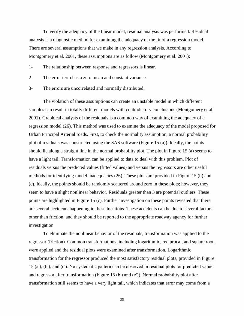
To verify the adequacy of the linear model, residual analysis was performed. Residual
analysis is a diagnostic method for examining the adequacy of the fit of a regression model.
There are several assumptions that we make in any regression analysis. According to
Montgomery et al. 2001, these assumptions are as follow (Montgomery et al. 2001):
1- The relationship between response and regressors is linear.
2- The error term has a zero mean and constant variance.
3- The errors are uncorrelated and normally distributed.
The violation of these assumptions can create an unstable model in which different
samples can result in totally different models with contradictory conclusions (Montgomery et al.
2001). Graphical analysis of the residuals is a common way of examining the adequacy of a
regression model (26). This method was used to examine the adequacy of the model proposed for
Urban Principal Arterial roads. First, to check the normality assumption, a normal probability
plot of residuals was constructed using the SAS software (Figure 15 (a)). Ideally, the points
should lie along a straight line in the normal probability plot. The plot in Figure 15 (a) seems to
have a light tail. Transformation can be applied to data to deal with this problem. Plot of
residuals versus the predicted values (fitted values) and versus the regressors are other useful
methods for identifying model inadequacies (26). These plots are provided in Figure 15 (b) and
(c). Ideally, the points should be randomly scattered around zero in these plots; however, they
seem to have a slight nonlinear behavior. Residuals greater than 3 are potential outliers. These
points are highlighted in Figure 15 (c). Further investigation on these points revealed that there
are several accidents happening in these locations. These accidents can be due to several factors
other than friction, and they should be reported to the appropriate roadway agency for further
investigation.
To eliminate the nonlinear behavior of the residuals, transformation was applied to the
regressor (friction). Common transformations, including logarithmic, reciprocal, and square root,
were applied and the residual plots were examined after transformation. Logarithmic
transformation for the regressor produced the most satisfactory residual plots, provided in Figure
15 (a′), (b′), and (c′). No systematic pattern can be observed in residual plots for predicted value
and regressor after transformation (Figure 15 (b′) and (c′)). Normal probability plot after
transformation still seems to have a very light tail, which indicates that error may come from a
39
distribution that has a slightly lighter tail than a normal distribution. Because there is no evidence
of model inadequacy, we can conclude that the transformation was satisfactory.
Norm
al C
umul
ative
Dist
ribut
ion
0.0
0.2
0.4
0.6
0.8
1.0
CDF of RSTUDENT0.0 0.1 0.2 0.3 0.4 0.5 0.6 0.7 0.8 0.9 1.0
(a) Normal probability plot (NPP) before
transformation
Norm
al C
umul
ative
Dist
ribut
ion
0.0
0.2
0.4
0.6
0.8
1.0
CDF of RSTUDENT0.0 0.1 0.2 0.3 0.4 0.5 0.6 0.7 0.8 0.9 1.0
(a′) Normal probability plot (NPP) after transformation
Stud
entiz
ed R
esid
ual w
ithou
t Cur
rent
Obs
-2
-1
0
1
2
3
4
Predicted Value0.8 1.0 1.2 1.4 1.6 1.8 2.0 2.2 2.4 2.6
(b) Residual plot for predicted values
St
uden
tized
Res
idua
l with
out C
urre
nt O
bs
-2
-1
0
1
2
3
4
Predicted Value1.0 1.2 1.4 1.6 1.8 2.0 2.2 2.4 2.6 2.8
(b′) Residual plot for predicted values after
transformation (x → Ln(x))
Stud
entiz
ed R
esid
ual w
ithou
t Cur
rent
Obs
-2
-1
0
1
2
3
4
SN20 25 30 35 40 45 50 55 60 65
(c) Residual plot for regressor
Stud
entiz
ed R
esid
ual w
ithou
t Cur
rent
Obs
-2
-1
0
1
2
3
4
logSN2.8 3.0 3.2 3.4 3.6 3.8 4.0 4.2
(c′) Residual plot for regressor after transformation (x →
Ln(x)) Figure 15 Residual plots.
Potential Outlier
40

Once the transformations were verified, ANOVA was conducted on the transformed
model. ANOVA results are provided in Table 3. It can be seen from the table that transformation
has improved the model’s coefficient of determination (R-square). The regressor in the model is
still satisfactory (P-value < 0.0001).
Table 3 Analysis of Variance (ANOVA) on Transformed Model for Urban Principle Arterial Roads
Analysis of Variance
Source DF Sum of Squares
Mean Square F Value Pr > F
Model 1 5.77753 5.77753 115.97 <.0001 Error 21 1.04624 0.04982 Corrected Total 22 6.82377 Root MSE Dependent Mean Coeff Var R-Square Adj R-Sq 0.22321 1.71191 13.0384 0.8467 0.8394
Parameter Estimates
Variable DF Parameter Estimate
Standard Error t Value Pr > |t| 95% Confidence
Limits Intercept 1 7.11387 0.50379 14.12 <.0001 6.06619 8.16155 Ln(SN) 1 -1.46691 0.13622 -10.77 <.0001 -1.75019 -1.18363
Similar analysis was performed for other road classes. Proper transformation was applied
for each model.
Table 4 summarizes the model’s parameters. According to P-values, friction is a
significant factor in all the models except for Urban Freeway Expressway wet-condition crashes
(in which P-value > 0.05). The slope of the regression line is negative for all cases except for
Urban Freeway Expressway dry-condition crashes. It is noted that the coefficient of
determination for this type of roadway is very low. This supports the hypothesis that increasing
the friction level decreases the rate of both dry- and wet-condition car crashes.
41
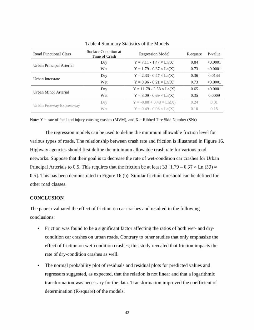
Table 4 Summary Statistics of the Models
Road Functional Class Surface Condition at Time of Crash Regression Model R-square P-value
Urban Principal Arterial Dry Y = 7.11 - 1.47 × Ln(X) 0.84 <0.0001 Wet Y = 1.79 - 0.37 × Ln(X) 0.73 <0.0001
Urban Interstate Dry Y = 2.33 - 0.47 × Ln(X) 0.36 0.0144 Wet Y = 0.96 - 0.21 × Ln(X) 0.73 <0.0001
Urban Minor Arterial Dry Y = 11.78 - 2.58 × Ln(X) 0.65 <0.0001 Wet Y = 3.09 - 0.69 × Ln(X) 0.35 0.0009
Urban Freeway Expressway Dry Y = -0.88 + 0.43 × Ln(X) 0.24 0.01 Wet Y = 0.49 - 0.08 × Ln(X) 0.10 0.15
Note: Y = rate of fatal and injury-causing crashes (MVM), and X = Ribbed Tire Skid Number (SNr)
The regression models can be used to define the minimum allowable friction level for
various types of roads. The relationship between crash rate and friction is illustrated in Figure 16.
Highway agencies should first define the minimum allowable crash rate for various road
networks. Suppose that their goal is to decrease the rate of wet-condition car crashes for Urban
Principal Arterials to 0.5. This requires that the friction be at least 33 [1.79 – 0.37 × Ln (33) ≈
0.5]. This has been demonstrated in Figure 16 (b). Similar friction threshold can be defined for
other road classes.
CONCLUSION
The paper evaluated the effect of friction on car crashes and resulted in the following
conclusions:
• Friction was found to be a significant factor affecting the ratios of both wet- and dry-
condition car crashes on urban roads. Contrary to other studies that only emphasize the
effect of friction on wet-condition crashes; this study revealed that friction impacts the
rate of dry-condition crashes as well.
• The normal probability plot of residuals and residual plots for predicted values and
regressors suggested, as expected, that the relation is not linear and that a logarithmic
transformation was necessary for the data. Transformation improved the coefficient of
determination (R-square) of the models.
42

Factors such as seasonal variation and temperature changes can also affect the friction
measurement. This effect needs to be further investigated and incorporated into the pavement
friction management program. Furthermore, the relationship between friction and crash rates can
be used by DOTs and highway agencies to define acceptable levels of friction for various types
of roadways in their networks.
ACHNOWLEDGEMENT
The authors would like to acknowledge the New Jersey Department of Transportation and, in
particular, Susan Gresavage for their contribution and support in providing the data for this
study, as well as Dr. Feng Guo for his guidance in the statistical analysis.
43
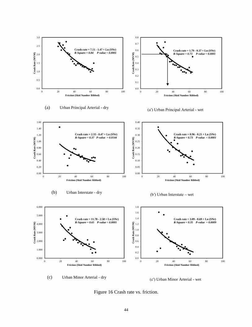
0.0
0.5
1.0
1.5
2.0
2.5
3.0
0 20 40 60 80 100
Cra
sh R
ate
(MV
M)
Friction (Skid Number Ribbed)
Crash rate = 7.11 - 1.47 × Ln (SNr)R-Square = 0.84 P-value < 0.0001
(a) Urban Principal Arterial - dry
0.0
0.1
0.2
0.3
0.4
0.5
0.6
0.7
0.8
0 20 40 60 80 100
Cra
sh R
ate
(MV
M)
Friction (Skid Number Ribbed)
Crash rate = 1.79 - 0.37 × Ln (SNr)R-Square = 0.73 P-value < 0.0001
(a′) Urban Principal Arterial - wet
0.00
0.20
0.40
0.60
0.80
1.00
1.20
1.40
1.60
0 20 40 60 80 100
Cra
sh R
ate
(MV
M)
Friction (Skid Number Ribbed)
Crash rate = 2.33 - 0.47 × Ln (SNr)R-Square = 0.37 P-value = 0.0144
(b) Urban Interstate - dry
0.00
0.05
0.10
0.15
0.20
0.25
0.30
0.35
0.40
0 20 40 60 80 100
Cra
sh R
ate
(MV
M)
Friction (Skid Number Ribbed)
Crash rate = 0.96 - 0.21 × Ln (SNr)R-Square = 0.73 P-value < 0.0001
(b′) Urban Interstate – wet
0.000
1.000
2.000
3.000
4.000
5.000
6.000
0 20 40 60 80 100
Cra
sh R
ate
(MV
M)
Friction (Skid Number Ribbed)
Crash rate = 11.78 - 2.58 × Ln (SNr)R-Square = 0.65 P-value < 0.0001
(c) Urban Minor Arterial - dry
0.0
0.2
0.4
0.6
0.8
1.0
1.2
1.4
1.6
1.8
0 20 40 60 80 100
Cra
sh R
ate
(MV
M)
Friction (Skid Number Ribbed)
Crash rate = 3.09 - 0.69 × Ln (SNr)R-Square = 0.35 P-value = 0.0009
(c′) Urban Minor Arterial - wet
Figure 16 Crash rate vs. friction.
44
REFERENCES
Bazlamit, S. M., and F. Reza. “Changes in Asphalt Pavement Friction Components and
Adjustment of Skid Number for Temperature”. Journal of Transportation Engineering, 131,
2005, pp. 470–476.
Bianchini, A., M. Heitzman, and S. Maghsoodloo. “Evaluation of Temperature Influence on
Friction Measurements”. Journal of Transportation Engineering, 137, 2011, pp. 640–647.
Davies, R. B., P. D. Cenek, and R. J. Henderson. “The Effect of Skid Resistance and Texture on
Crash Risk”. Paper presented at the International Conference on Surface Friction for Roads and
Runways, Christchurch, NZ, 2005.
FHWA. Technical Advisory T5040.38, “Pavement Friction Management”. Federal Highway
Administration, 2010. http://www.fhwa.dot.gov/pavement/t504038.cfm. Accessed July 30, 2013.
Flintsch, G. W., and K. K. McGhee. “NCHRP Synthesis 401: Quality Management of Pavement
Condition Data Collection”. Transportation Research Board, National Research Council,
Washington, D.C., 2009.
Flintsch, G. W., K. K. McGhee, E. de León Izeppi, and S. Najafi. “The Little Book of Tire
Pavement Friction”. Surface Properties Consortium, 2012.
https://secure.hosting.vt.edu/www.apps.vtti.vt.edu/1-
pagers/CSTI_Flintsch/The%20Little%20Book%20of%20Tire%20Pavement%20Friction.pdf.
Accessed July 30, 2013.
Fwa, T. F. “The Handbook of Highway Engineering”. CRC Press, Taylor and Francis Group,
2005.
Gan, A., K. Haleem, P. Alluri, and D. Saha. “Standardization of Crash Analysis in Florida,
Technical Report No. 1214”. Department of Transportation Office of University Research, 2012.
Gonzalez, O. D. “Evaluation of Pavement Surface Friction Seasonal Variations”. Virginia
Polytechnic Institute and State University, 2009. http://scholar.lib.vt.edu/theses/available/etd-
02082009-174223/unrestricted/Thesis2009-02-20.pdf. Accessed July 30, 2012.
45
Hall, J. W., K. L. Smith, L. Titus‐Glover, J. C. Wambold, T. J. Yager, and Z. Rado. “Guide for
Pavement Friction”. National Cooperative Highway Research Program, Transportation Research
Board of the National Academies, 2009.
Henry, J. J. “Evaluation of Pavement Friction Characteristics: A Synthesis of Highway Practice”,
NCHRP Synthesis 291. Transportation Research Board, National Research Council,
Washington, D.C., 2000.
Hill, B. J., and J. J. Henry. “Short-Term, Weather-Related Skid Resistance Variations”.
Transportation Research Record, No. 1654, Transportation Research Board of the National
Academics, Washington, D.C., 1981, pp. 76–81.
Ivey, D. L., L. I. Griffin III, J. R. Lock, and D. L. Bullard. “Texas Skid Initiated Accident
Reduction Program”, Final Report, Research Report 910-1F, TTI: 2-18-89/910, TX-92/910-1F.
Texas Department of Transportation, Austin, Texas, 1992.
Jayawickrama, P., and B. Thomas. “Correction of Field Skid Measurements for Seasonal
Variations in Texas”. Transportation Research Record, No. 1639, Transportation Research Board
of the National Academics, Washington, D.C., 1998, pp. 147–152.
Kulakowski, B. T., and D. W. Harwood. “Effect of Water-Film Thickness on Tire-Pavement
Friction”. Surface Characteristics of Roadways: International Research and Technologies,
American Society for Testing and Materials, 1990, pp. 50–60.
Kuttesch, J. S. “Quantifying the Relationship Between Skid Resistance and Wet Weather
Accidents for Virginia Data”. Virginia Polytechnic Institute and State University, 2004.
http://scholar.lib.vt.edu/theses/available/etd-10312004-
081948/unrestricted/Kuttesch_ThesisFinal.pdf. Accessed July 30, 2013.
Larson, R. M., T. E. Hoerner, K. D. Smith, and A. S. Wolterss. “Relationship Between Skid
Resistance Numbers Measured with Ribbed and Smooth Tire and Wet Accident Locations”.
Prepared for Ohio Department of Transportation office of Research and Development, 2008.
http://www.dot.state.oh.us/Divisions/Planning/SPR/Research/reportsandplans/Reports/2008/Pave
ment/ODOT%20134323%20-%20FINAL%20Report.pdf. Accessed July 30, 2013.
46

Montgomery, D. C., E. A. Peck, G. G. Vining, and J. Vining. “Introduction to Linear Regression
Analysis”. Wiley, New York, 2001.
Najafi, S., G. W. Flintsch, and K. K. McGhee. “Assessment of Operational Characteristics of
Continuous Friction Measuring Equipment (CFME)”. International Journal of Pavement
Engineering, Vol. 14, No. 8, 2013, pp. 706–714.
Roa, J. A. “Evaluation of International Friction Index and High Friction Surfaces”. Virginia
Polytechnic Institute and State University, 2008. http://scholar.lib.vt.edu/theses/available/etd-
12182008-225503/unrestricted/Thesis.pdf. Accessed July 30, 2013.
Rose, J. G., and B. M. Gallaway. “Water Depth Influence on Pavement Friction”. Transportation
Engineering Journal 103, 1997, pp. 491–506.
Schram, S. “Specifications for Aggregate Frictional Qualities in Flexible Pavements”. In
Transportation Research Record: Journal of the Transportation Research Board No. 2209,
Transportation Research Board of the National Academics, Washington, D.C., 2011, pp. 18–25.
Shahin, M. Y. “Pavement Management for Airports, Roads, and Parking Lots”. Springer Science
Business Media, LLC, 2005.
Viner, H., R. Sinhal, and A. Parry. “Linking Road Traffic Accidents with Skid Resistance-
Recent UK Developments”. TRL Paper reference PA/INF4520/05, 2005.
Viner, H., R. Sinhal, and T. Parry. “Review of UK Skid Resistance Policy”. In Symposium on
Pavement Surface Characteristics [of Roads and Airports], 5th, 2004, Toronto, Ontario, Canada,
2004.
Wambold, J. C., J. Henry, C. Antle, B. Kulakowski, W. Meyer, A. Stocker, J. Button, and D.
Anderson. “Pavement Friction Measurement Normalized for Operational, Seasonal, and Weather
Effects”. Pennsylvania State University, Pennsylvania Transportation Institute, 1987.
47

CHAPTER 3 - PAVEMENT FRICTION MANAGEMENT – ARTIFICIAL
NEURAL NETWORK APPROACH4
Abstract
The Highway Safety Improvement Program (HSIP) requires state highway agencies to improve
their roadway network safety through a ‘strategic’ and ‘data-driven’ approach. As part of HSIP,
the Federal Highway Administration (FHWA) mandates that states develop a Pavement Friction
Management (PFM) System to reduce the rate of fatal and injury-causing crashes and prioritize
their safety improvement projects based on the crash risk. This paper aims to predict the rate of
wet and dry vehicle crashes based on surface friction, traffic level, and speed limit using an
artificial neural network (ANN). Three learning algorithms, Levenberg-Marquardt, conjugate
gradient, and resilient back-propagation, were examined to train the network. Levenberg-
Marquardt produced the best precision and was used to develop the model. The results of the
study suggest that the ANN model can reliably predict the rate of crashes. The prediction model
can be used as a scale to prioritize safety improvement projects based on the rate of fatal and
injury-causing crashes.
4 This manuscript will be submitted to the International Journal of Pavement Engineering (IJPE) for publication. Co-authors include: Gerardo Flintsch, and Seyedmeysam Khaleghian.
48

INTRODUCTION
The ‘Moving Ahead for Progress in the 21st Century Act (MAP-21)’ was signed into law on July
6, 2012, and went into effect on October 1, 2012, (United States Department of Transportation
2013). MAP-21 ‘continued the Highway Safety Improvement Program (HSIP) as a core Federal-
aid program’ (FHWA 2014). The goal of HSIP is to reduce traffic fatalities and serious injuries.
As part of HSIP, the Federal Highway Administration (FHWA) has established measures for
state highway agencies to assess the rate of fatal and injury-causing crashes (Federal Highway
Administration 2014). HSIP project selection is based on ‘crash experience, crash potential, or
other data supported means as identified by the State, and establishes the relative severity of
those locations’ (Federal Highway Administration 2010). To establish criteria to prioritize
projects for HSIP funds, states should implement a pavement friction management (PFM)
program (Federal Highway Administration 2010). PFM allows states to incorporate safety into
their asset management decision making process. Locations with high risk of fatal and injury-
causing crashes are identified and corrective measures taken to address friction deficiencies in
those locations. Projects can be prioritized based on the crash risk.
In 2009, the American Association of State Highway and Transportation Officials
(AASHTO) published the Guide for Pavement Friction to provide guidelines for state highway
agencies to develop and implement a PFM program (Hall et al. 2009). The AASHTO guide
suggests three methods to define investigatory and intervention levels for friction. The methods
provided in the AASHTO guide are based on traditional regression analysis. This paper
investigates the suitability of one of the methods provided by the AASHTO guide to be
implemented in PFM and it proposes an alternative approach based on an artificial neural
network (ANN) to model the relationship between friction and crashes. The proposed method
can be used as a scale to prioritize projects for safety improvements.
BACKGROUND
The effect of tire-pavement friction on the rate of vehicle crashes is well known among
researchers (Flintsch et al. 2012). Several researchers have attempted to define an acceptable
level of friction at which the rate of crashes will be minimized. Rizenbergs et al. (1972) did a
friction study on rural interstate routes in Kentucky using a ribbed-tire locked-wheel friction
49
tester. They found that wet crash rates as well as wet-to-dry crash ratios increased once the
friction numbers dropped below 40 (Rizenbergs et al. 1972). McCullough and Hankins (1996)
studied the relationship between friction and crashes for 571 sites in Texas. The result of the
study revealed that the majority of crashes happened on the sites with low friction, while a few
crashes happened on the sites with high friction values. They proposed a minimum desirable
friction threshold of 0.4 measured at 30 mph (McCullough and Hankins 1966).
The AASHTO Guide for Pavement Friction has defined three methods to establish two
distinctive friction threshold levels, investigatory level and intervention level. Sites with friction
values below the investigatory level will be selected for detailed investigation to determine if
there is a need for posting warning signs. Sites with friction values below the intervention level
will be selected for corrective action, such as resurfacing or other programmatic maintenance
treatment. The first AASHTO method uses the friction deterioration curve by plotting friction
loss versus pavement age. The friction value at which significant loss rapidly begins is selected
as the investigatory level. The intervention level is defined at a fixed percentage below
investigatory level (Figure 17) (Hall et al. 2009).
Figure 17 Friction deterioration curve (after Hall et al. (2009)).
The second AASHTO method uses both the friction deterioration curve and historical
crash data. The investigatory level is set where there is a significant drop in friction level and the
50
intervention method is set where there is a significant increase in crashes (Figure 18) (Hall et al.
2009).
Figure 18 Investigatory and intervention friction level based on friction deterioration and crash rate (after Hall et al. (2009)).
The third AASHTO method uses the friction distribution and crash rate for each roadway
category to determine the investigatory and intervention levels of friction. The histogram of
pavement friction and wet-to-dry crash ratio is plotted first (Figure 19). The mean and standard
deviation of the friction distribution are then calculated. The investigatory level is set as the
mean friction minus X (e.g., 1.5 or 2.0) standard deviations and it is adjusted to where wet-to-dry
crashes begin to increase considerably. The intervention level is set as the mean friction minus Y
(e.g., 2.5 or 3.0) standard deviations and it is adjusted to a minimum satisfactory wet-to-dry crash
rate or by the point where enough funding is available to address the friction deficiencies (Hall et
al. 2009). This method is more robust than other two approaches since an agency can adjust the
intervention friction level based on available funding.
51
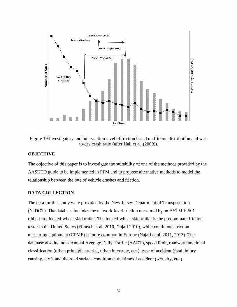
Figure 19 Investigatory and intervention level of friction based on friction distribution and wet-to-dry crash ratio (after Hall et al. (2009)).
OBJECTIVE
The objective of this paper is to investigate the suitability of one of the methods provided by the
AASHTO guide to be implemented in PFM and to propose alternative methods to model the
relationship between the rate of vehicle crashes and friction.
DATA COLLECTION
The data for this study were provided by the New Jersey Department of Transportation
(NJDOT). The database includes the network-level friction measured by an ASTM E-501
ribbed-tire locked-wheel skid trailer. The locked-wheel skid trailer is the predominant friction
tester in the United States (Flintsch et al. 2010, Najafi 2010), while continuous friction
measuring equipment (CFME) is more common in Europe (Najafi et al. 2011, 2013). The
database also includes Annual Average Daily Traffic (AADT), speed limit, roadway functional
classification (urban principle arterial, urban interstate, etc.), type of accident (fatal, injury-
causing, etc.), and the road surface condition at the time of accident (wet, dry, etc.).
52
Fatal and injury-causing crashes for various urban roads were used for this study. The
total number of wet and dry, fatal and injury-causing vehicle crashes, as well as average speed
limit for each roadway type, is provided in Table 5.
Table 5 Fatal and injury-causing accident counts (after Najafi et al. 2014).
Number of sites with accidents
Functional Class Surface
Condition
Speed Limit (kph)
Dry Wet Min Max Urban Principal Arterial
20308 5010 40 88
Urban Interstate
3963 1251 56 104 Urban Minor Arterial
2979 714 40 88
Urban Freeway Expressway 2409 665 40 104
DATA ANALYSIS
The first two methods suggested by the AASHTO guide require historical friction data, which
was not available for this study. Thus, the authors tested only the third method. Friction numbers
were grouped into bins with two-unit increments (i.e., 20 < FN ≤ 22, etc.). The friction and crash
data were then matched using route and milepost information. If the distance between the
location of the crash and the measured friction was less than 0.1 miles, the data were matched.
The total numbers of friction sites for each bin, as well as the ratio of wet-to-dry fatal and injury-
causing crashes for each friction bin, were then calculated. The summary of data is provided in
Table 6.
53
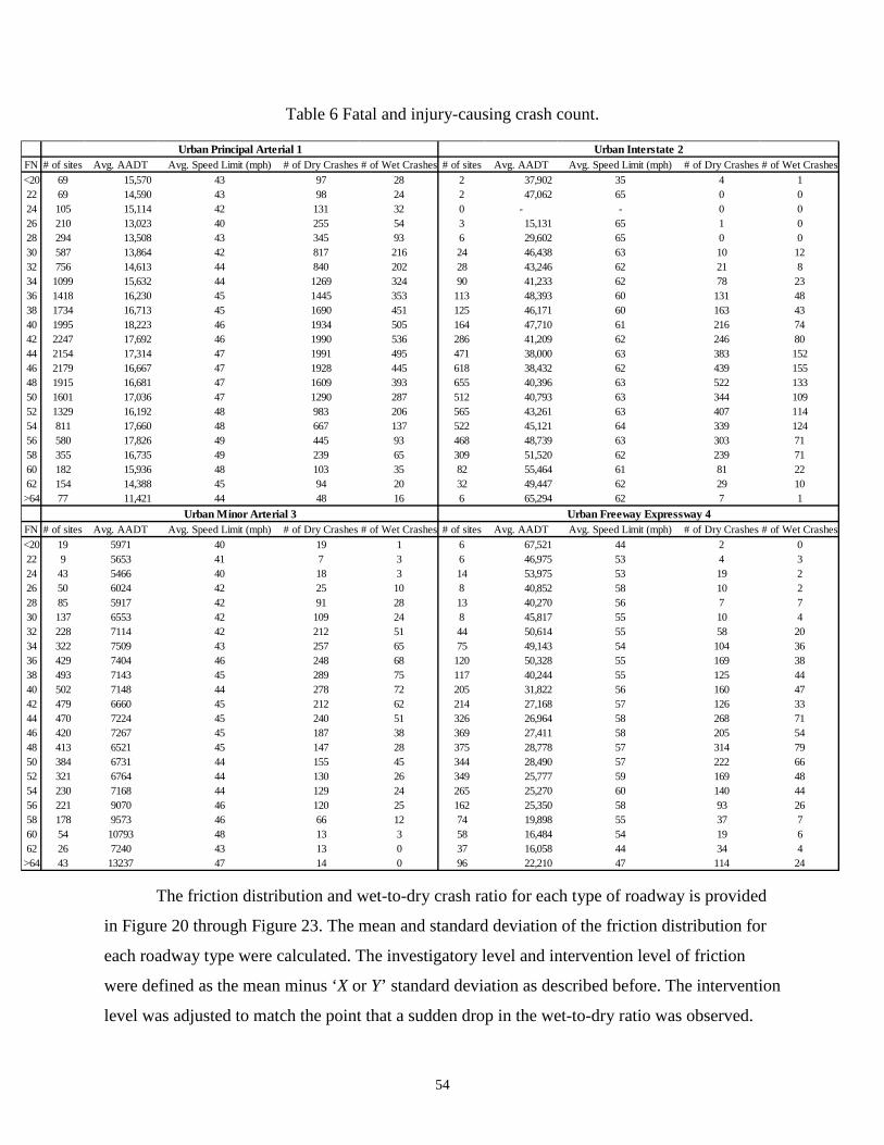
FN # of sites Avg. AADT Avg. Speed Limit (mph) # of Dry Crashes # of Wet Crashes # of sites Avg. AADT Avg. Speed Limit (mph) # of Dry Crashes # of Wet Crashes<20 69 15,570 43 97 28 2 37,902 35 4 122 69 14,590 43 98 24 2 47,062 65 0 024 105 15,114 42 131 32 0 - - 0 026 210 13,023 40 255 54 3 15,131 65 1 028 294 13,508 43 345 93 6 29,602 65 0 030 587 13,864 42 817 216 24 46,438 63 10 1232 756 14,613 44 840 202 28 43,246 62 21 834 1099 15,632 44 1269 324 90 41,233 62 78 2336 1418 16,230 45 1445 353 113 48,393 60 131 4838 1734 16,713 45 1690 451 125 46,171 60 163 4340 1995 18,223 46 1934 505 164 47,710 61 216 7442 2247 17,692 46 1990 536 286 41,209 62 246 8044 2154 17,314 47 1991 495 471 38,000 63 383 15246 2179 16,667 47 1928 445 618 38,432 62 439 15548 1915 16,681 47 1609 393 655 40,396 63 522 13350 1601 17,036 47 1290 287 512 40,793 63 344 10952 1329 16,192 48 983 206 565 43,261 63 407 11454 811 17,660 48 667 137 522 45,121 64 339 12456 580 17,826 49 445 93 468 48,739 63 303 7158 355 16,735 49 239 65 309 51,520 62 239 7160 182 15,936 48 103 35 82 55,464 61 81 2262 154 14,388 45 94 20 32 49,447 62 29 10
>64 77 11,421 44 48 16 6 65,294 62 7 1
FN # of sites Avg. AADT Avg. Speed Limit (mph) # of Dry Crashes # of Wet Crashes # of sites Avg. AADT Avg. Speed Limit (mph) # of Dry Crashes # of Wet Crashes<20 19 5971 40 19 1 6 67,521 44 2 022 9 5653 41 7 3 6 46,975 53 4 324 43 5466 40 18 3 14 53,975 53 19 226 50 6024 42 25 10 8 40,852 58 10 228 85 5917 42 91 28 13 40,270 56 7 730 137 6553 42 109 24 8 45,817 55 10 432 228 7114 42 212 51 44 50,614 55 58 2034 322 7509 43 257 65 75 49,143 54 104 3636 429 7404 46 248 68 120 50,328 55 169 3838 493 7143 45 289 75 117 40,244 55 125 4440 502 7148 44 278 72 205 31,822 56 160 4742 479 6660 45 212 62 214 27,168 57 126 3344 470 7224 45 240 51 326 26,964 58 268 7146 420 7267 45 187 38 369 27,411 58 205 5448 413 6521 45 147 28 375 28,778 57 314 7950 384 6731 44 155 45 344 28,490 57 222 6652 321 6764 44 130 26 349 25,777 59 169 4854 230 7168 44 129 24 265 25,270 60 140 4456 221 9070 46 120 25 162 25,350 58 93 2658 178 9573 46 66 12 74 19,898 55 37 760 54 10793 48 13 3 58 16,484 54 19 662 26 7240 43 13 0 37 16,058 44 34 4
>64 43 13237 47 14 0 96 22,210 47 114 24
Urban Principal Arterial 1 Urban Interstate 2
Urban Minor Arterial 3 Urban Freeway Expressway 4
Table 6 Fatal and injury-causing crash count.
The friction distribution and wet-to-dry crash ratio for each type of roadway is provided
in Figure 20 through Figure 23. The mean and standard deviation of the friction distribution for
each roadway type were calculated. The investigatory level and intervention level of friction
were defined as the mean minus ‘X or Y’ standard deviation as described before. The intervention
level was adjusted to match the point that a sudden drop in the wet-to-dry ratio was observed.
54
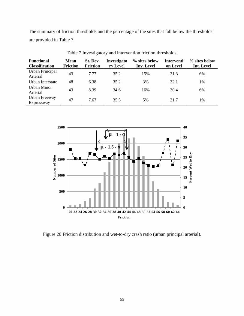
The summary of friction thresholds and the percentage of the sites that fall below the thresholds
are provided in Table 7.
Table 7 Investigatory and intervention friction thresholds.
Functional Classification
Mean Friction
St. Dev. Friction
Investigatory Level
% sites below Inv. Level
Intervention Level
% sites below Int. Level
Urban Principal Arterial 43 7.77 35.2 15% 31.3 6%
Urban Interstate 48 6.38 35.2 3% 32.1 1% Urban Minor Arterial 43 8.39 34.6 16% 30.4 6%
Urban Freeway Expressway 47 7.67 35.5 5% 31.7 1%
0
5
10
15
20
25
30
35
40
0
500
1000
1500
2000
2500
20 22 24 26 28 30 32 34 36 38 40 42 44 46 48 50 52 54 56 58 60 62 64
Perc
ent W
et to
Dry
Num
ber
of S
ites
Friction
µ - 1 × σ
µ - 1.5 × σ
Figure 20 Friction distribution and wet-to-dry crash ratio (urban principal arterial).
55
0
20
40
60
80
100
120
140
0
100
200
300
400
500
600
700
20 22 24 26 28 30 32 34 36 38 40 42 44 46 48 50 52 54 56 58 60 62 64
Perc
ent W
et to
Dry
Num
ber
of S
ites
Friction
µ - 2 × σ
µ - 2.5 × σ
Figure 21 Friction distribution and wet-to-dry crash ratio (urban interstate).
0
5
10
15
20
25
30
35
40
45
0
100
200
300
400
500
600
20 22 24 26 28 30 32 34 36 38 40 42 44 46 48 50 52 54 56 58 60 62 64
Perc
ent W
et to
Dry
Num
ber
of S
ites
Friction
µ - 1 × σ
µ - 1.5 × σ
Figure 22 Friction distribution and wet-to-dry crash ratio (urban minor arterial).
56
0
20
40
60
80
100
120
0
50
100
150
200
250
300
350
400
20 22 24 26 28 30 32 34 36 38 40 42 44 46 48 50 52 54 56 58 60 62 64
Perc
ent W
et to
Dry
Num
ber
of S
ites
Friction
µ - 1.5 × σ
µ - 2 × σ
Figure 23 Friction distribution and wet-to-dry crash ratio (urban freeway expressway).
High variability with some peak crash rates can be observed for low friction numbers.
For all cases except urban principal arterial roads, a significant drop in the wet-to-dry crash ratios
was observed around friction number 32. However, no clear trend can be observed for wet-to-dry
crash ratios for urban principal arterial roads, which account for the majority of the network. A
previous study by the authors showed a significant relationship between both wet and dry crash
ratio and friction that can explain the lack of relationship between the wet-to-dry crash ratio and
friction (Najafi et al. 2014). It should also be noted that there are only a few sites with extremely
low (and high) friction values. Defining friction threshold based on a small sample size may not
be appropriate.
To consider the effect of wet and dry crashes separately, the wet and dry crash rate for
each interval was computed by dividing the crash count by exposure (Gan et al. 2012):
LYnAADT
crashesofNumberExposure
crashesofNumberRateCrash××××⋅⋅
=×⋅⋅
=⋅000,000,1000,000,1
(6)
where
AADT: total AADT (averaged for each bin)
57
n: wet or dry time exposure
Y: study duration in years
L: length of the roadway segments.
Weather information was extracted from the National Oceanic and Atmospheric
Administration (NOAA) database (2015).The crash rates were then normalized between zero and
one for each roadway type and crash type (wet or dry):
)()(
)(RateCrashMINRateCrashMAX
RateCrashMINRateCrashRateCrashNormalized i
i ⋅−⋅⋅−⋅
=⋅⋅ (7)
where Normalized Crash Rate(i) corresponds to the normalized crash rate for the ith friction bin.
In a previous study, the authors used linear regression to model the relationship between the
crash rate and friction (Najafi et al. 2015). In this study, ANN was implemented as an alternative
to model the relationship.
Artificial neural network (ANN)
ANN is a soft computing approach that is inspired by the way the human brain and nervous
system work (Khdair 2006). ANN’s processing system consists of several ‘interconnected’
cells—known as neurons—that work harmonious to solve a problem. The pattern and strength of
connectivity between neurons encrypt the knowledge of a network. Similar to a human’s brain,
ANN can learn by example, and it can be trained to predict an unknown system or behavior.
ANN can make generalizations, and it is very suitable in cases for which many examples are
available (Flintsch and Chen 2004). ANN is known to be capable of extracting complex
nonlinear relationships between multiple variables (Somers and Casal, 2009).
ANN has been successfully implemented in the past to support infrastructure asset
management decisions (Flintsch and Chen 2004). Flintsch et al. (1998) used ANN to select
pavement candidates for preservation. Suman and Sinha (2012) and Thube (1997) developed a
pavement condition forecasting model using ANN. The effectiveness of ANN in accident
prediction modeling has also been confirmed by several researchers (Moghaddam et al. 2011,
Duddu and Pulugurtha 2012, Kunt et al. 2012, Jafari et al. 2013). Moghaddam et al. (2011) used
58

ANN to model the relationship between human factors, road, vehicle, weather conditions, traffic
volume, and speed flow on the severity level of crashes on urban. Kunt et al. (2012) predicted the
severity level of crashes on a freeway using ANN.
One of the main benefits of the ANN approach is that it can work with uncertain and
incomplete data. Furthermore, it can learn from examples. This is particularly appealing at the
early stages of friction management program development. The system can be established with
limited data and improved over time as more data become available. The main disadvantage of
ANN is that it behaves like a ‘black box’, which makes it hard to understand.
ANN’s structure consists of input, hidden layers, and output layers (Shekharan 1998).
The number of layers in an ANN depends on the number of hidden layers. Each layer contains
several interconnected neurons. Each neuron has an output, which relates to its activation level,
and it can spread out to other neurons. A simple schematic of neuron function is illustrated in
Figure 24 (Khdair 2006).
Figure 24 Neuron model (after Khdair 2006).
Input signals are received by neurons and are given a weight and summed. This can be
mathematically expressed as follows (Moghaddam et al. 2011):
)( ii
iiji
netfXxwnet
=
=∑ (8)
Where,
59

f is the threshold activation function
Xi is the output signal
xi is the input signal, and
wij is the weight’s coefficient from the i-th neuron of the first layer to the j-th neuron of
the second layer.
Threshold function is typically nonlinear. On a simple from for discrete neural networks
it can be expressed by the step function (Khdair 2006):
<−=
>
=010)(01
)( /
xxxfx
xf (9)
where f′(x) is the previous value of f(x) and X is the summation of the input neuron’s activation
as defined in Equation 8. For non-discrete networks, threshold function can be expressed in
sigmoidal form (Khdair 2006):
( ) xexf −+=
11 (10)
where f(x) is the threshold activation function.
The input data are propagated through the network to generate outputs. The outputs are
then compared with the target values to calculate the error. Using a back-propagation learning
algorithm, the connection weights are modified to minimize the target error. Basically, the back-
propagation algorithm uses the rule repeatedly to calculate the effect of each connection weight
with respect to the error. This can be mathematically expressed as follows (Riedmiller and Braun
1993):
ij
i
i
i
iij wnet
netX
XE
wE
∂∂
∂∂
∂∂
=∂∂
(11)
where E is the error function.
60

Once the partial derivate for the entire network’s connection weight is calculated, the
error function is minimized using a simple gradient descent (Riedmiller and Braun 1993):
)()()1( twEtwtw
ijijij ∂
∂−=+ ε (12)
where
wij(t) is the weight coefficient in step t, from neuron i to neuron j, and
ε is the learning coefficient.
The training process continues unit the error reaches its desired values after many steps
(epochs). The time needed to reach the desired values is directly affected by how learning rate (ε)
is selected. If the learning rate is set too small, many epochs are needed to reach coverage. On
the other hand, if learning rate is set too high, then the network may learn too quickly and may
not learn very well or at all if there is a lot of variation in the data. One way to cope with this
issue is to introduce a momentum term (Riedmiller and Braun 1993):
)1()()( −∆+∂∂
−=∆ twtwEtw ij
ijij αε (13)
where α is the momentum parameter.
The momentum parameter scales the effect of previous step (t) on the current step (t+1). It is
believed that the momentum term makes the learning procedure more stable; however, in
practice this is not always the case. In fact, finding an optimum value for the momentum
parameter is as problematic as finding an optimum value for learning rate (Riedmiller and Braun
1993). To overcome the disadvantages of a gradient-descent-based back-propagation algorithm,
several alternative learning algorithms have been proposed over the years. Levenberg-Marquardt,
conjugate gradient, and resilient back-propagation algorithms were examined in this study to
train the network. The algorithm with the best performance was selected to develop the final
model. All training networks work in a similar fashion as they attempt to reduce the global error
by adjusting the weights.
61

Levenberg-Marquardt algorithm
The Levenberg-Marquardt algorithm can approach second-order timing speed without the need
to calculate a Hessian matrix. The gradient descent in Equation 11 can be expressed as follows:
eJg T= (14)
where
e is the error vector, and
J is the Jacobian matrix of the first derivatives of the network errors (ijw
E∂∂
).
To minimize the gradient descent, the second order partial derivative must be taken,
which requires calculating the Hessian matrix. Calculating the Hessian matrix is typically very
time-consuming. In the Levenberg-Marquardt algorithm, the Hessian matrix for performance
function, in the form of a sum of squares, can be approximated as follows (Kisi and Uncuoglu
2005):
JJH T= (15)
Calculating the Jacobian matrix is much simpler than calculating the Hessian matrix as it
can be calculated through a standard back-propagation technique. The Levenberg-Marquardt
algorithm uses a Newton-like update to approximate the Hessian matrix (Kisi and Uncuoglu
2005):
( ) eJIJJww TTtt
11
−
+ +−= m (16)
where
µ is always positive and called the combination coefficient, and
I is the identity matrix.
This turns into Newton’s method when μ is zero, and it turns into the gradient descent with a
small step size when μ is large. μ is initialized to be large and it is decreased after each successful
62

step, which results in reduction in the performance function. μ is only increased if a tentative step
increased the performance function. This allows the solution to converge quickly to the local
minimum. The goal is to shift to Newton’s method as quickly as possible since it is faster and
more accurate near a minimum error (Kisi and Uncuoglu 2005).
Conjugate gradient algorithm
The back-propagation algorithm adjust the weights in the steepest descent direction (the most
negative gradient), which is the direction that the performance function is decreasing most
rapidly. This approach does not produce the fastest convergence. The conjugate gradient
algorithms search along the conjugate direction, which generally results in a faster convergence
than the steepest descent directions (Kisi and Uncuoglu 2005).
Generally, the step size is adjusted at each iteration, and a search is made along the
conjugate gradient direction in order to find the step size that minimizes the performance
function. The first iteration starts by searching the steepest descent direction (Kisi and Uncuoglu
2005):
00 gp −= (17)
A line search is performed in order to find the optimal distance to move along the current search
direction (Kisi and Uncuoglu. 2005):
kkkk gxx α+=+1 (18)
The next search direction is considered to be conjugate to the previous search direction,
which is generally done by combining the new steepest descent direction with the previous
search direction (Kisi and Uncuoglu 2005):
1−+−= kkkk pgp β (19)
where βk is the ratio of the norm squared on the current gradient to the norm squared on the
previous gradient (Kisi and Uncuoglu 2005):
63

11 −−
=k
Tk
kTk
k gggg
β (20)
Resilient back-propagation algorithm
A resilient back-propagation algorithm modifies the weight step based on gradient information to
make the convergence faster. The magnitude of the weight update ( ij∆ ) is determined by an
adaptive update value, which evolves during the learning process, based on the following rules:
∆
<∂∂
∂∂
∆
>∂∂
∂∂
∆
=∆
−
−−−
−−+
elsewE
wEif
wE
wEif
tij
t
ij
t
ij
tij
t
ij
t
ij
tij
tij
,
0,
0,
)1(
)()1()1(
)()1()1(
)( η
η
(21)
where +− <<< ηη 10 .
If the partial derivative of the weight changes its sign, it means the last update was too
big and the algorithm has passed the local minimum. In that case, the update value ( ij∆ ) is
decreased by the factor −η . On the other hand, if the derivative retains its sign, the update value
will be slightly increased by the factor +η to accelerate convergence. The weight update can be
determined based on update values (Riedmiller and Braun 1993):
<∂∂
∆+
>∂∂
∆−
=∆
elsewEif
wEif
wt
ij
tij
t
ij
tij
tij
,0
0,
0,
)()(
)()(
)( (22)
and
64

)()()1( tij
tij
tij www ∆+=+ (23)
If the derivate is positive, it means the error is increasing, so in that case the weight is
decreased by the update value. If the derivative is negative, the weight will be increased by the
update value. As explained before, if the partial derivate changes sign, it means the last update
was too big and the local minimum was missed. In that case the previous weight update is
revised (Riedmiller and Braun 1993):
0,)()1(
)1()( <∂∂
∂∂
∆−=∆−
−t
ij
t
ij
tij
tij w
EwEifww (24)
The slopes of sigmoidal functions, which are often used as transfer functions, approach
zero as the input gets very large. This causes issues when using the steepest gradient descent to
train the network as a gradient’s magnitude can be very small and result in very small changes in
weights even though they are far from optimum. The resilient back-propagation algorithm is only
dependent on the sign of the partial derivate, and the magnitude of the derivate has no effect on
the weight update, which makes it more efficient than a pure gradient descent-based back-
propagation method (Kisi and Uncuoglu 2005).
Selection of Learning Algorithm
The MATLAB software package was used to develop and train the ANN. The data were
randomly divided into three sets: 70% of data were used to train the network, 15% were used to
validate the network, and 15% were used to test the network. The validation data set is used to
determine a stopping point for the learning algorithm and the test data set is used to assess the
performance of the trained network outside the training set. The inputs to the model are Roadway
Functional Classification, friction number, AADT, and speed limit. The output was dry or wet
normalized crash rate. The mean squared error (MSE) between the network’s outputs and the
targets was used as a measure of prediction accuracy of the trained network. The number of
neurons in the hidden layer was increased to minimize the MSE. All three learning algorithms
were used to train the network. The network with one hidden layer with eight neurons produced
a satisfactory MSE for predicting both wet and dry normalized crash rate. The MSE and training
65

time for each network is provided in Table 8. The Levenberg-Marquardt algorithm had the
highest prediction accuracy (lowest MSE) and the fastest convergence time, and it was selected
for further analysis.
Table 8 Comparison of learning algorithms.
Dry Crash Prediction Wet Crash Prediction
MSE Training Time (s) MSE Training Time (s)
Learning Algorithm Levenberg-Marquardt 0.006 0.988 0.016 0.447 Conjugate gradient 0.023 1.04 0.031 0.546 Resilient back-propagation 0.011 1.677 0.025 0.574
First, the validation performance of the network was evaluated. Figure 25 depicts the
ANN’s validation performance for dry crashes. As explained before, an epoch is the process of
providing the network with inputs and updating the weights for all the neurons within the
network. The error in training data decreases as the network learns. Generally, several epochs are
needed to train the ANN. Training stops once the validation error stops decreasing. The epoch
corresponding to this error is called the optimum epoch number (5 in this case). The error on the
test data indicates how well the network will respond to the new data set.
Figure 25 Validation performance for dry crashes.
66
The distribution of the errors is shown in Figure 26. Most errors are close to zero. Ideally,
the errors should be tightly grouped around zero. The error distribution can be improved by
adding more neurons to the hidden layer. In this case, the number of neurons and error seem to
be satisfactory.
Figure 26 Error distribution for dry crashes.
To have a visual comparison, the regression plots of the outputs are provided in Figure 27
and Figure 28. Ideally, each point should fit close to the unity (dotted) line. Any points far from
the group indicate potential outliers and may require further investigation. Regression lines show
how well the outputs correlate with the targets. The regression line should follow close to the
dotted line. The overall distance between the dotted line and regression line is summarized by the
R value, which should ideally be close to 1.
67
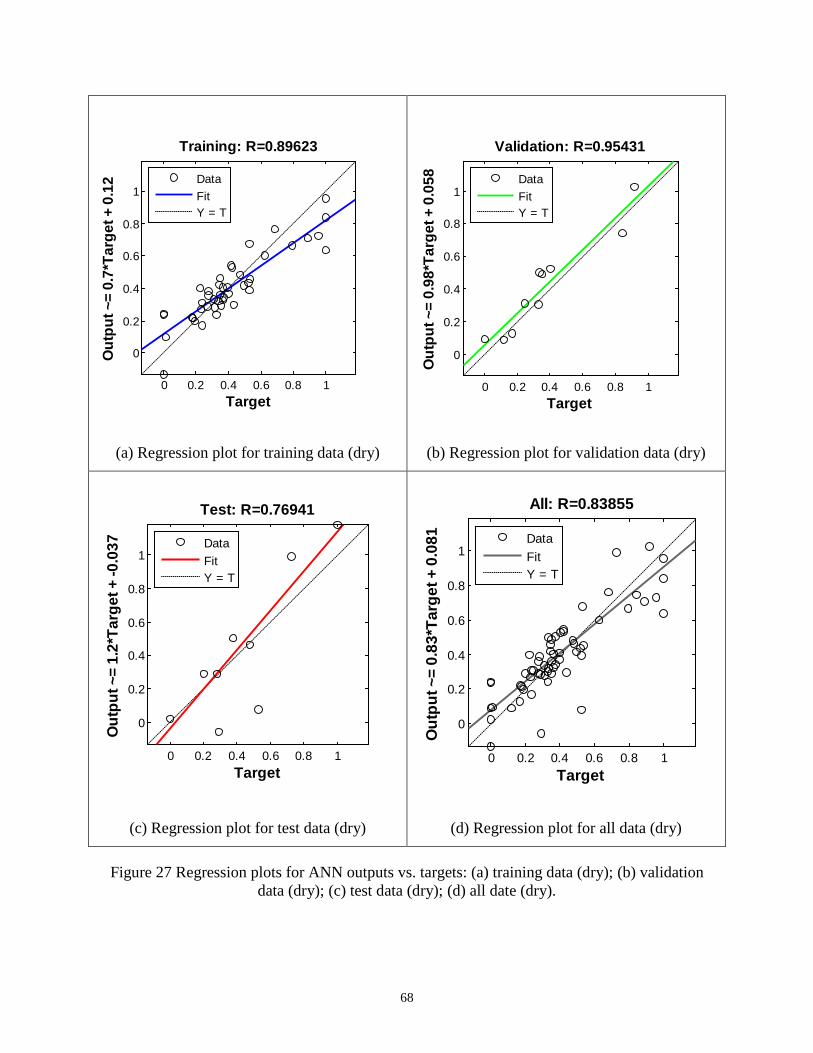
0 0.2 0.4 0.6 0.8 1
0
0.2
0.4
0.6
0.8
1
Target
Out
put ~
= 0.
7*Ta
rget
+ 0
.12
Training: R=0.89623
DataFitY = T
(a) Regression plot for training data (dry)
0 0.2 0.4 0.6 0.8 1
0
0.2
0.4
0.6
0.8
1
TargetO
utpu
t ~=
0.98
*Tar
get +
0.0
58
Validation: R=0.95431
DataFitY = T
(b) Regression plot for validation data (dry)
0 0.2 0.4 0.6 0.8 1
0
0.2
0.4
0.6
0.8
1
Target
Out
put ~
= 1.
2*Ta
rget
+ -0
.037
Test: R=0.76941
DataFitY = T
(c) Regression plot for test data (dry)
0 0.2 0.4 0.6 0.8 1
0
0.2
0.4
0.6
0.8
1
Target
Out
put ~
= 0.
83*T
arge
t + 0
.081
All: R=0.83855
DataFitY = T
(d) Regression plot for all data (dry)
Figure 27 Regression plots for ANN outputs vs. targets: (a) training data (dry); (b) validation data (dry); (c) test data (dry); (d) all date (dry).
68
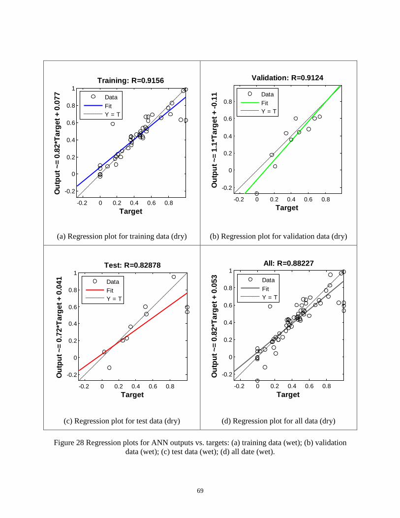
-0.2 0 0.2 0.4 0.6 0.8
-0.2
0
0.2
0.4
0.6
0.8
1
Target
Out
put ~
= 0.
82*T
arge
t + 0
.077
Training: R=0.9156
DataFitY = T
(a) Regression plot for training data (dry)
-0.2 0 0.2 0.4 0.6 0.8
-0.2
0
0.2
0.4
0.6
0.8
TargetO
utpu
t ~=
1.1*
Targ
et +
-0.1
1
Validation: R=0.9124
DataFitY = T
(b) Regression plot for validation data (dry)
-0.2 0 0.2 0.4 0.6 0.8
-0.2
0
0.2
0.4
0.6
0.8
1
Target
Out
put ~
= 0.
72*T
arge
t + 0
.041
Test: R=0.82878
DataFitY = T
(c) Regression plot for test data (dry)
-0.2 0 0.2 0.4 0.6 0.8
-0.2
0
0.2
0.4
0.6
0.8
1
Target
Out
put ~
= 0.
82*T
arge
t + 0
.053
All: R=0.88227
DataFitY = T
(d) Regression plot for all data (dry)
Figure 28 Regression plots for ANN outputs vs. targets: (a) training data (wet); (b) validation data (wet); (c) test data (wet); (d) all date (wet).
69
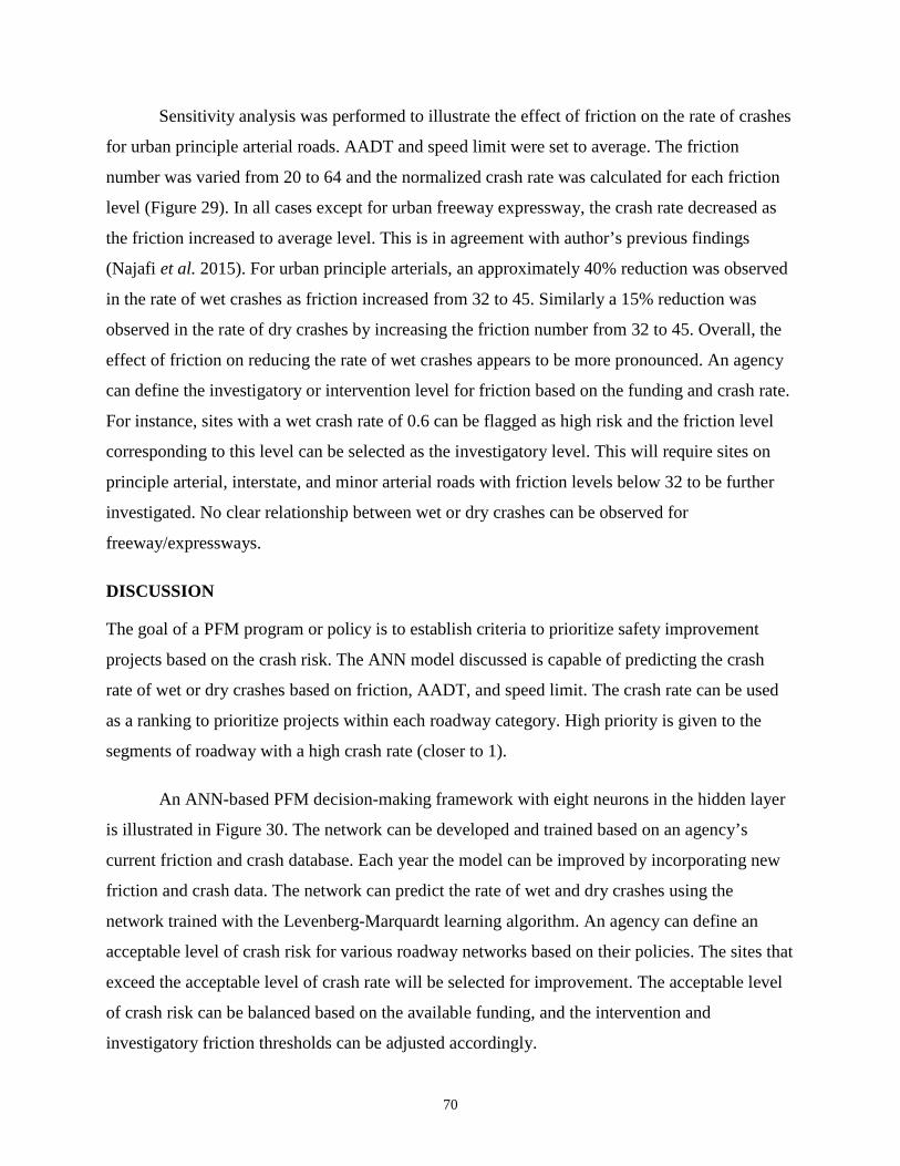
Sensitivity analysis was performed to illustrate the effect of friction on the rate of crashes
for urban principle arterial roads. AADT and speed limit were set to average. The friction
number was varied from 20 to 64 and the normalized crash rate was calculated for each friction
level (Figure 29). In all cases except for urban freeway expressway, the crash rate decreased as
the friction increased to average level. This is in agreement with author’s previous findings
(Najafi et al. 2015). For urban principle arterials, an approximately 40% reduction was observed
in the rate of wet crashes as friction increased from 32 to 45. Similarly a 15% reduction was
observed in the rate of dry crashes by increasing the friction number from 32 to 45. Overall, the
effect of friction on reducing the rate of wet crashes appears to be more pronounced. An agency
can define the investigatory or intervention level for friction based on the funding and crash rate.
For instance, sites with a wet crash rate of 0.6 can be flagged as high risk and the friction level
corresponding to this level can be selected as the investigatory level. This will require sites on
principle arterial, interstate, and minor arterial roads with friction levels below 32 to be further
investigated. No clear relationship between wet or dry crashes can be observed for
freeway/expressways.
DISCUSSION
The goal of a PFM program or policy is to establish criteria to prioritize safety improvement
projects based on the crash risk. The ANN model discussed is capable of predicting the crash
rate of wet or dry crashes based on friction, AADT, and speed limit. The crash rate can be used
as a ranking to prioritize projects within each roadway category. High priority is given to the
segments of roadway with a high crash rate (closer to 1).
An ANN-based PFM decision-making framework with eight neurons in the hidden layer
is illustrated in Figure 30. The network can be developed and trained based on an agency’s
current friction and crash database. Each year the model can be improved by incorporating new
friction and crash data. The network can predict the rate of wet and dry crashes using the
network trained with the Levenberg-Marquardt learning algorithm. An agency can define an
acceptable level of crash risk for various roadway networks based on their policies. The sites that
exceed the acceptable level of crash rate will be selected for improvement. The acceptable level
of crash risk can be balanced based on the available funding, and the intervention and
investigatory friction thresholds can be adjusted accordingly.
70

0
0.1
0.2
0.3
0.4
0.5
0.6
0.7
0.8
0.9
1
20 22 24 26 28 30 32 34 36 38 40 42 44 46 48 50 52 54 56 58 60 62 64
Nor
mal
ized
Cra
sh R
ate
Friction
Urban Principal Arterial Urban InterstateUrban Minor Arterial Urban Freeway Expressway
(a) Dry crashes
0
0.1
0.2
0.3
0.4
0.5
0.6
0.7
0.8
0.9
1
20 22 24 26 28 30 32 34 36 38 40 42 44 46 48 50 52 54 56 58 60 62 64
Nor
mal
ized
Cra
sh R
ate
Friction
Urban Principal Arterial Urban InterstateUrban Minor Arterial Urban Freeway Expressway
(b) Wet crashes Figure 29 ANN-predicted normalized crash rate vs. friction: (a) dry crashes; (b) wet crashes.
Investigatory Level
71
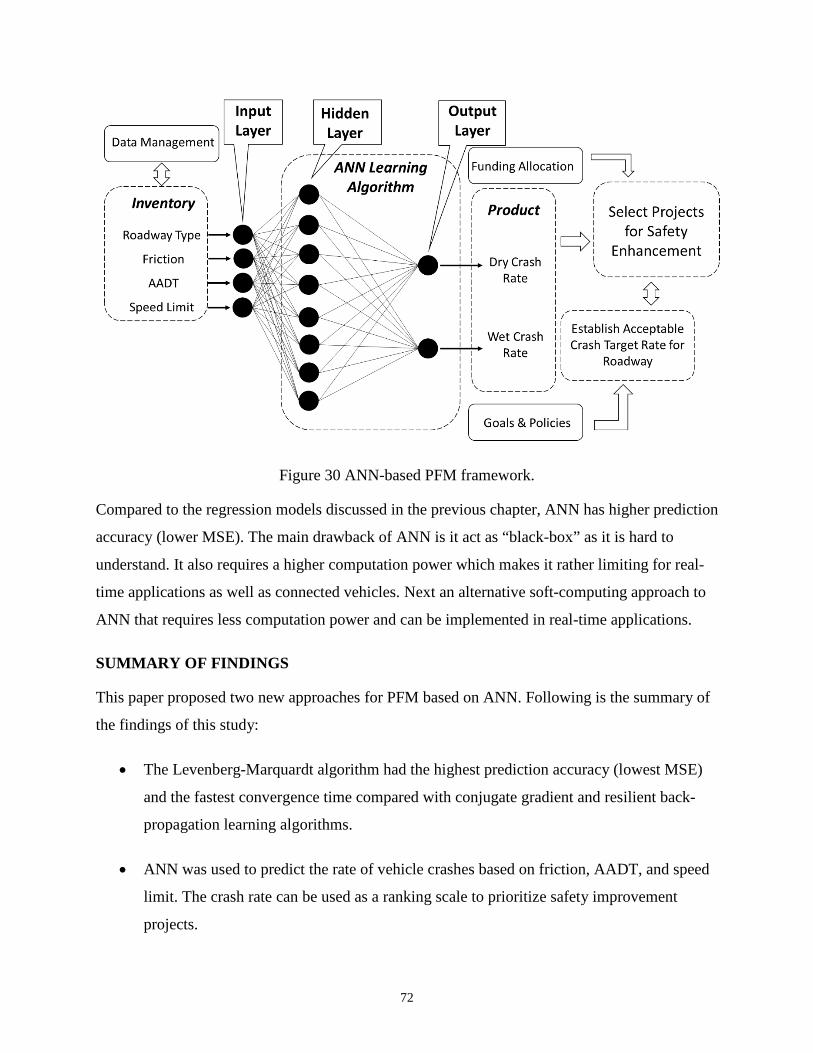
Figure 30 ANN-based PFM framework.
Compared to the regression models discussed in the previous chapter, ANN has higher prediction
accuracy (lower MSE). The main drawback of ANN is it act as “black-box” as it is hard to
understand. It also requires a higher computation power which makes it rather limiting for real-
time applications as well as connected vehicles. Next an alternative soft-computing approach to
ANN that requires less computation power and can be implemented in real-time applications.
SUMMARY OF FINDINGS
This paper proposed two new approaches for PFM based on ANN. Following is the summary of
the findings of this study:
• The Levenberg-Marquardt algorithm had the highest prediction accuracy (lowest MSE)
and the fastest convergence time compared with conjugate gradient and resilient back-
propagation learning algorithms.
• ANN was used to predict the rate of vehicle crashes based on friction, AADT, and speed
limit. The crash rate can be used as a ranking scale to prioritize safety improvement
projects.
72
• The rate of wet crashes observed for site with friction number below 32 was 40 percent
higher than sites with friction higher than networks average (45). In case of dry crashes,
15 percent higher crash rate was observed for sites with friction number below 32
compared to sites with friction level above average.
• The effect of friction on reducing the rate of wet crashes is more pronounced than dry
crashes.
CONCLUSIONS
The learning ability of the proposed approach makes it appealing for developing a PFM
compared with traditional statistical approaches because it can be developed from a limited
database. The prediction accuracy of the network can be improved by incorporating more data
into the system. The model can be updated every year at the end of the friction data collection
cycle.
ACKNOWLEDGMENTS
The authors would like to acknowledge the New Jersey Department of Transportation and, in
particular Susan Gresavage, for their contribution and support in providing the data for this
study.
REFERENCES
Duddu, V. and Pulugurtha, S., 2012. “Neural networks to estimate crashes at zonal level for
transportation planning”. In: European Transport Conference 2012, 8–10 October 2012,
Glasgow, Scotland. London: Association for European Transport.
Federal Highway Administration, 2010. “Technical Advisory 5040.38” [online]. Available from:
https://www.fhwa.dot.gov/pavement/t504038.cfm [accessed 28 December 2014].
Federal Highway Administration, 2014. “Highway Safety Improvement Program (HSIP)”
[online]. Available from: http://safety.fhwa.dot.gov/hsip/ [accessed 3 January 2015].
Flintsch G.W., J. Zaniewski, Delton J, and A. Medina, 1998. “Artificial neural network based
project selection level pavement management system”. In: 4th International Conference on
73

Managing Pavements, 17–21 May 1998, Durbin, South Africa. Pretoria: University of South
Africa, 451–464.
Flintsch, G.W., K. K. McGhee, E. de León Izeppi, and S. Najafi, 2010. “Speed adjustment
factors for locked-wheel skid trailer measurements”. Transportation Research Record: Journal of
the Transportation Research Board, 2155, 117–123.
Flintsch, G.W., K. K. McGhee, E. de León Izeppi, and S. Najafi, 2012. “The little book of tire
pavement friction” [online]. Available from:
https://secure.hosting.vt.edu/www.apps.vtti.vt.edu/1-
pagers/CSTI_Flintsch/The%20Little%20Book%20of%20Tire%20Pavement%20Friction.pdf
[Accessed 30 July 2013].
Flintsch, G.W., and Chen, C., 2004. “Soft computing application in infrastructure management”.
Journal of Infrastructure Systems, 10, 157–166.
Gan, A., K. Haleem, P. Alluri, and D. Saha, 2012. “Standardization of crash analysis in Florida”.
Tallahassee, FL: Florida Department of Transportation, Contract No. BDK80 977-10.
Hall, J.W., K. L. Smith, L. Titus‐Glover, J. C. Wambold, T. J. Yager, and Z. Rado, 2009. “Guide
for pavement friction”. Washington, DC: National Cooperative Highway Research Program,
Transportation Research Board of the National Academies.
Hastie, T., Tibshirani, R., and J. Friedman, 2009. “Elements of statistical learning”. New York:
Springer-Verlag.
Jafari S.A., Jahandideh S, Jahandideh M, E.B. Asadabadi, 2013. “Prediction of road traffic death
rate using neural networks optimised by genetic algorithm”. International Journal of Injury
Control and Safety Promotion [online]. DOI: 10.1080/17457300.2013.857695.
Khdair, R.M., 2006. “Signature recognition using neural network”. Master’s Thesis. Near East
University, Nicosia.
Kisi, O., and Uncuoglu, E., 2005. “Comparison of three back-propogation training algorithms for
two case studies”. Indian Journal of Engineering & Materials Science, 12, 434–442.
74

Kunt, M.M., Aghayana, I., and Noiib, N., 2012. “Prediction for traffic accident severity:
Comparing the artificial neural network, genetic algorithm, combined genetic algorithm and
pattern search methods”. Transport, 26 (4), 353–366, DOI: 10.3846/16484142.2011.635465.
McCullough, B.V., and Hankins, K.D., 1966. “Skid resistance guidelines for surface
improvements on Texas highways”. Highway Research Record, 131, 204–217.
Moghaddam F.R., Afandizadeh, Sh., and Ziyadi, M., 2011. “Prediction of accident severity using
artificial neural networks”. International Journal of Civil Engineering, 9 (1), 41–48.
Najafi, S., 2010. “Evaluation of continuous friction measuring equipment (CFME) for supporting
pavement friction management programs” [online]. Thesis. Virginia Polytechnic Institute and
State University. Available from: http://scholar.lib.vt.edu/theses/available/etd-12132010-
111100/unrestricted/Najafi_Shahriar_2010.pdf [Accessed 15 February 2015].
Najafi, S., G. W. Flintsch, E. de León Izeppi, K. K. McGhee, and S. Katicha, 2011.
“Implementation of cross-correlation to compare continuous friction measuring equipment
(CFME)”. In: Transportation Research Board 90th Annual Meeting Compendium of Papers
DVD, 23–27 January 2011, Washington, DC. Washington, DC: Transportation Research Board,
Paper No. 11-2083.
Najafi, S., Flintsch, G.W., and McGhee, K.K., 2013. “Assessment of operational characteristics
of continuous friction measuring equipment (CFME)”. International Journal of Pavement
Engineering, 14 (8), 706–714.
Najafi, S., Flintsch, G.W., and Medina, A., 2014. “Case study on the evaluation of the effect of
tire-pavement friction on the rate of roadway crashes”. In: Transportation Research Board 93rd
Annual Meeting Compendium of Papers [DVD], 12–16 January 2014, Washington, DC.
Washington, DC: Transportation Research Boartd, Paper No. 14-5617.
Najafi, S., Flintsch, G.W., and Medina, A., 2015. “Linking roadway crashes and tire–pavement
friction: A case study”. International Journal of Pavement Engineering [online]. DOI:
10.1080/10298436.2015.1039005.
75

National Oceanic and Atmospheric Administration, 2015. “Climate data online: Dataset
discovery” [online]. Available from: www.ncdc.noaa.gov/cdo-web/datasets [accessed 30 August
2015].
Riedmiller, M., and Braun, H., 1993. “A direct adaptive method for faster backpropagation
learning: The RPROP algorithm”. In: IEEE International Conference on Neural Networks, 28
March–1 April 1993, San Francisco, CA. New York: IEEE, 586–591. DOI:
10.1109/ICNN.1993.298623
Rizenbergs, R.L., Burchett, J.L., and Napier, C.T., 1972. “Skid resistance of pavements, Part II”.
Lexington, Kentucky: Kentucky Department of Highways, Report No. KYHPR-64-24.
Shekharan, A.R., 1998. “Effect of noisy data on pavement performance prediction by artificial
neural networks”. Transportation Research Record, 1643, 7–13.
Somers, M., and Casal, J., 2009. “Using artificial neural networks to model nonlinearity: The
case of the job satisfaction–job performance relationship”. Organizational Research Methods, 12,
(3), 403–417. DOI: 10.1177/1094428107309326.
Suman S.K., and Sinha, S., 2012. “Pavement condition forecasting through artificial neural
network modelling”. International Journal of Emerging Technology and Advanced Engineering,
2 (11).
Thube, D.T, 1997. “Artificial neural network (ANN) based pavement deterioration models for
low volume roads in India”. Int. J. Pavement Res. Technol., 5 (2), 115–120.
United States Department of Transportation, 2013. “Moving Ahead for Progress in the 21st
Century Act (MAP-21)” [online]. Available from: http://www.dot.gov/map21 [accessed 3
January 2015].
76
CHAPTER 4 – DEVELOPING A PAVEMENT FRICTION MANAGEMENT
(PFM) FRAMEWORK UZINF FUZZY LOGIC5
ABSTRACT
Minimizing roadway crashes and fatalities is one of the primary objectives of highway engineers,
and can be achieved in part through appropriate maintenance practices. Maintaining an
appropriate level of friction is a crucial maintenance practice, due to the effect it has on roadway
safety. This paper presents a fuzzy logic inference system that predicts the rate of vehicle crashes
based on traffic level, speed limit, and surface friction. Mamdani and Sugeno fuzzy controllers
were used to develop the model. The application of the proposed fuzzy control system in friction
management is demonstrated. The results of this study provide a decision support model for
highway agencies to monitor their network’s friction and make appropriate judgments to correct
deficiencies based on crash risk.
5 This manuscript will be submitted to the Journal of Accident Analysis & Prevention for publication. Co-authors include: Gerardo Flintsch and Seyedmeysam Khaleghian.
77
INTRODUCTION
Friction is known to be an important factor affecting the risk of vehicle crashes (Flintsch et al.
2013; Henry 2000). Minimizing roadway crashes and fatalities is one of the Federal Highway
Administration’s (FHWA) and U.S. Department of Transportation’s (USDOT) top priorities
(FHWA 2014). The FHWA’s Highway Safety Improvement Program (HSIP) policy states that
‘each State shall develop, implement, and evaluate on an annual basis a HSIP that has the overall
objective of significantly reducing the occurrence of and the potential for fatalities and serious
injuries resulting from crashes on all public roads’ (FHWA T5040.38). Furthermore, HSIP
project locations shall be selected based on ‘crash experience, crash potential, or other data
supported means as identified by the State, and establishes the relative severity of those
locations’ (FHWA T5040.38). To achieve this to the greatest extent possible, State highway
agencies will require the development of a Pavement Friction Management (PFM) program.
The FHWA has implemented various policies throughout the years to minimize friction-
related vehicle crashes (Najafi et al. 2011). In 1980, the FHWA introduced the Skid Accident
Reduction Program (SARP) (FHWA T 5040.17). The goal of the SARP was to minimize wet-
weather skidding accidents. A subsequent publication supplied new guidelines for selecting
appropriate treatments to achieve optimum surface textures for providing a high level of wet
friction and a low level of tire-pavement noise (FHWA T5040.36). In 2010, the agency canceled
the SARP and introduced the PFM program (FHWA T5040.38). The new program introduces a
more proactive and systemic approach to identifying and correcting friction deficiencies and
prioritizing resources based on needs.
FHWA technical advisory T5040.36 and the American Association of State Highway and
Transportation Officials (AASHTO) Guide for Pavement Friction Management have presented
several approaches to defining minimum and desirable friction levels (Hall et al. 2009). Most
approaches require historical friction and accident data, which may not be readily available. In a
previous study, authors suggested using an Artificial Neural Network (ANN) to model the
relationship between friction and vehicle crashes and used the model to define a desirable
network level friction threshold. And while an ANN provides high prediction accuracy, it is also
hard to understand and typically requires high computational power. Fuzzy logic models, on the
78
other hand, are easy to understand and can be modified based on engineering judgment and
experts’ opinions. This makes them very appealing, since they can be modified based on an
agency’s needs.
BACKGROUND
Fuzzy logic systems are based on traditional rules-based expert systems and can use approximate
data and ‘linguistic rules’ to drive human-like decisions (Zadeh 1965). Experts’ opinions can be
incorporated into the fuzzy logic system through these linguistic rules (Flintsch et al. 2004). The
fuzzy logic inference system consists of a fuzzifier, fuzzy inference engine, fuzzy rules and
defuzzifier (Suman 2012).
The fuzzifier converts the numerical input values into linguistic variables. Several
linguistic sets can be defined for each variable. Input variables can partially belong to more than
one linguistic set. The belonging of any input variable to a certain linguistic set is defined as the
degree of membership to that set and can take any value in the [0, 1] interval (i.e., the degree of
membership will be zero if the value does not belong to the set) (Suman 2012). The inference
engine transforms the inputs into the linguistic set of output based on linguistic rules. Fuzzy rules
can be defined based on expert opinion or based on the observed relationship between the input
variables and the outputs. Finally, the defuzzifier converts the fuzzy output set to a single ‘crisp’
value (Suman 2012).
Over the last few years, several researchers have proposed a fuzzy decision-making
approach to determining pavement maintenance and safety needs based on various pavement
characteristics (Sandra et al. 2000; Chassiakos 2006; Chen 2007; Suman et al. 2012; Xiao et al.
2000). Sandra et al. developed a fuzzy logic-based decision making tool to prioritize pavement
needs based on the severity of various pavement distresses (Sandra et al. 2000). Chen used a
fuzzy approach to predict the life-cycle cost of various pavement maintenance strategies based
on pavement condition (Chen 2007). Both studies used expert opinion to develop fuzzy rules.
Xiao et al. used fuzzy-logic to predict the risk of wet pavement crashes (Xiao et al. 2000). The
researchers used accident and traffic data from 123 sections of highways in Pennsylvania,
collected from 1984 to 1986. Researchers’ results showed that fuzzy-logic can, indeed, be used
79
to predict the rate of crashes. Furthermore, they found that fuzzy-logic can also be used to
determine the corrective action(s) that should be taken to improve safety (Xiao et al. 2000).
OBJECTIVE
This paper uses a fuzzy logic inference system to model friction’s relationship to speed limit,
traffic volume, and crash rate. Mamdani and Sugeno fuzzy controllers are used to develop the
proposed model, which provides a reliable and customizable tool that agencies can use to
establish a relationship between crash rate and friction level and also employ as a scale to
prioritize safety projects based on crash risk. Furthermore, the model can be used in real-time
crash warning systems to alert drivers to potential slippery spots. The application of the proposed
fuzzy system in a real-time crash warning system is demonstrated as a proof of concept.
DATA COLLECTION
The data for this study were provided by the New Jersey Department of Transportation
(NJDOT). The friction data were collected every 0.16 kilometer (km) on more than 3,218 km of
urban principle arterial roads using an ASTM E-501 ribbed-tire locked-wheel skid trailer6
(Figure 31) (Najafi et al. 2014). The data also included crash location (route and milepost),
accident type (fatal, injury-causing, etc.), roadway surface condition at the time of accident (wet,
dry, etc.), annual average daily traffic (AADT), and speed limit. Weather information was
extracted from the National Oceanic and Atmospheric Administration (NOAA) database.
(NOAA, 2015).
6 The results of previous chapters showed promising relationship between friction and crash rate for Urban Principle Arterial roads. For this reason the database for this type of roadway were investigated in this chapter.
80

Figure 31 Locked-wheel skid trailer.
Only fatal and injury causing crashes were considered in the study. Overall, 20,308 dry-
condition and 5,010 wet-condition fatal and injury causing crashes were observed. To aggregate
the data, fictional numbers were divided into bins with two unit increments (20 < SN ≤ 22, 22 <
SN ≤ 24, etc.). The wet/dry crash distribution in relation to friction is illustrated in Figure 32.
0
500
1000
1500
2000
2500
20 22 24 26 28 30 32 34 36 38 40 42 44 46 48 50 52 54 56 58 60 62 64
Cra
sh C
ount
Friction
Dry CrashesWet Crashes
Figure 32 Crash distribution for fatal and injury causing crashes.
81
More dry-condition crashes were observed than wet-condition crashes. This is due to wet
time exposure. Also, more crashes were observed around the average friction range (40-46). This
necessitates normalizing the crashes based on friction distribution and wet time exposure. To
normalize the crashes, the crash rate was derived for each friction interval by dividing the crash
count by exposure (Gan et al. 2012):
(25)
Where,
AADT: total annual average daily traffic (vehicles per day [vpd])
n: wet or dry time exposure (days)
Y: study duration in years (year)
L: length of the roadway segments (km).
The crash rates were then normalized between 0 and 1 for each crash type (wet or dry):
(26)
Where Normalized Crash Rate(i) corresponds to the normalized crash rate for the ith
friction bin.
DATA ANALYSIS
MATLAB software was used to develop Mamdani and Sugeno fuzzy systems. The inputs to the
models are speed limit, traffic and friction and the output is wet or dry crash rate. The discussion
for each system is provided in the following sections.
Mamdani Fuzzy Inference System
The Mamdani fuzzy inference is one of the most widely used fuzzy inference systems. It was
proposed by Mamdani in 1975 to serve as a control system for a steam engine by utilizing sets of
linguistic rules that were determined from experts’ knowledge (Mamdani 1975). In the Mamdani
82
inference, inputs are first fuzzified using membership functions. Let’s assume X is a space of
points and the generic element of X is denoted by x (X = {x}). A membership function fA(x)
characterizes a fuzzy set of A in X in which each point in X is a real number in the [0,1] interval
and the values of fA(x) at x represent the degree of membership of x in A. If the value of fA(x) is
closer to 1, it means x has a higher degree of membership in A (Zadeh 1965). The most
commonly used membership function shapes include triangle, trapezoid, Gaussian, and
sigmoidal. This study used triangular membership functions. The distribution can be
mathematically expressed as follows:
(27)
Where a, b, and c are the x coordinates of the three corners of the triangle.
Membership Functions
Friction, speed limit, and AADT are the inputs of the system and the output is the wet or dry
crash rate. Friction was broken down into five levels: very low (less than 25), low (25 to 35),
medium (35 to 45), high (45 to 55), and very high (above 55). As previously discussed, the
degree of membership to each set is varied between 0 and 1. For example, in Figure 33, the
friction number 22’s degree of belonging (membership) to the very low group and low group are
75%, and 25% respectively. As a friction number increases, its degree of belonging to the low
friction group increases and so on. So at any friction level, we can incorporate some level of
uncertainty by overlapping the sets. Similar membership functions were defined for traffic and
speed limit. Traffic and speed limit were categorized into three levels: low, medium, and high, as
shown in Figure 34 and Figure 35.
Five levels of cash risk were also defined based on the crash rate: very low, low, medium,
high and very high (Figure 36 and Figure 37). The levels can be modified based on the agency’s
83
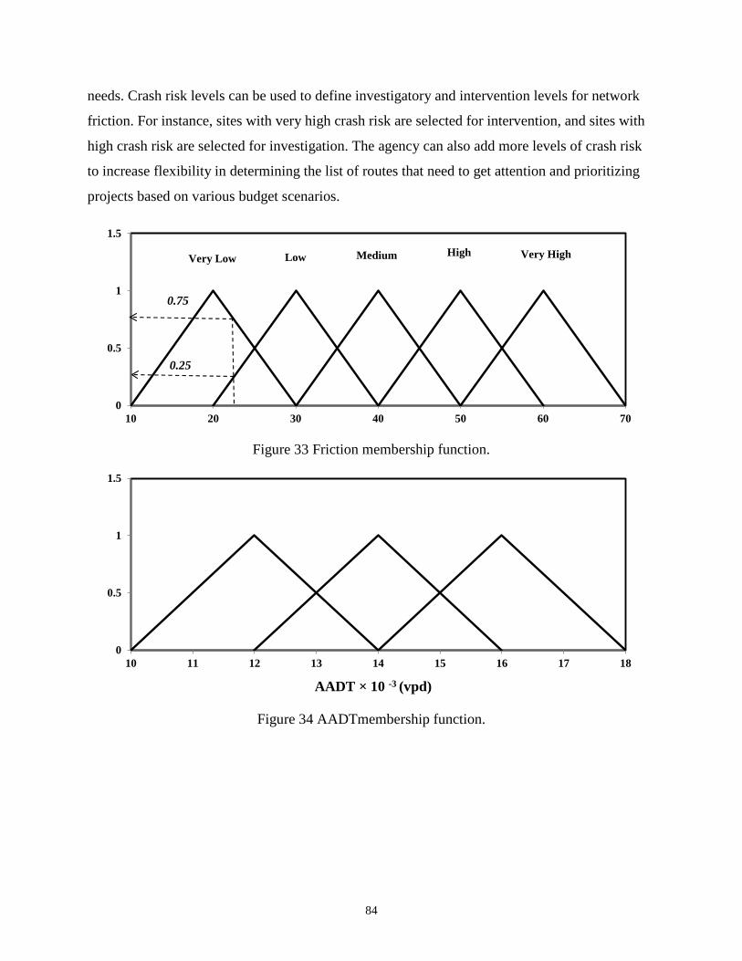
needs. Crash risk levels can be used to define investigatory and intervention levels for network
friction. For instance, sites with very high crash risk are selected for intervention, and sites with
high crash risk are selected for investigation. The agency can also add more levels of crash risk
to increase flexibility in determining the list of routes that need to get attention and prioritizing
projects based on various budget scenarios.
0
0.5
1
1.5
10 20 30 40 50 60 70
Very Low Low Medium High Very High
0.75
0.25
Figure 33 Friction membership function.
0
0.5
1
1.5
10 11 12 13 14 15 16 17 18
AADT × 10 -3 (vpd)
Figure 34 AADTmembership function.
84
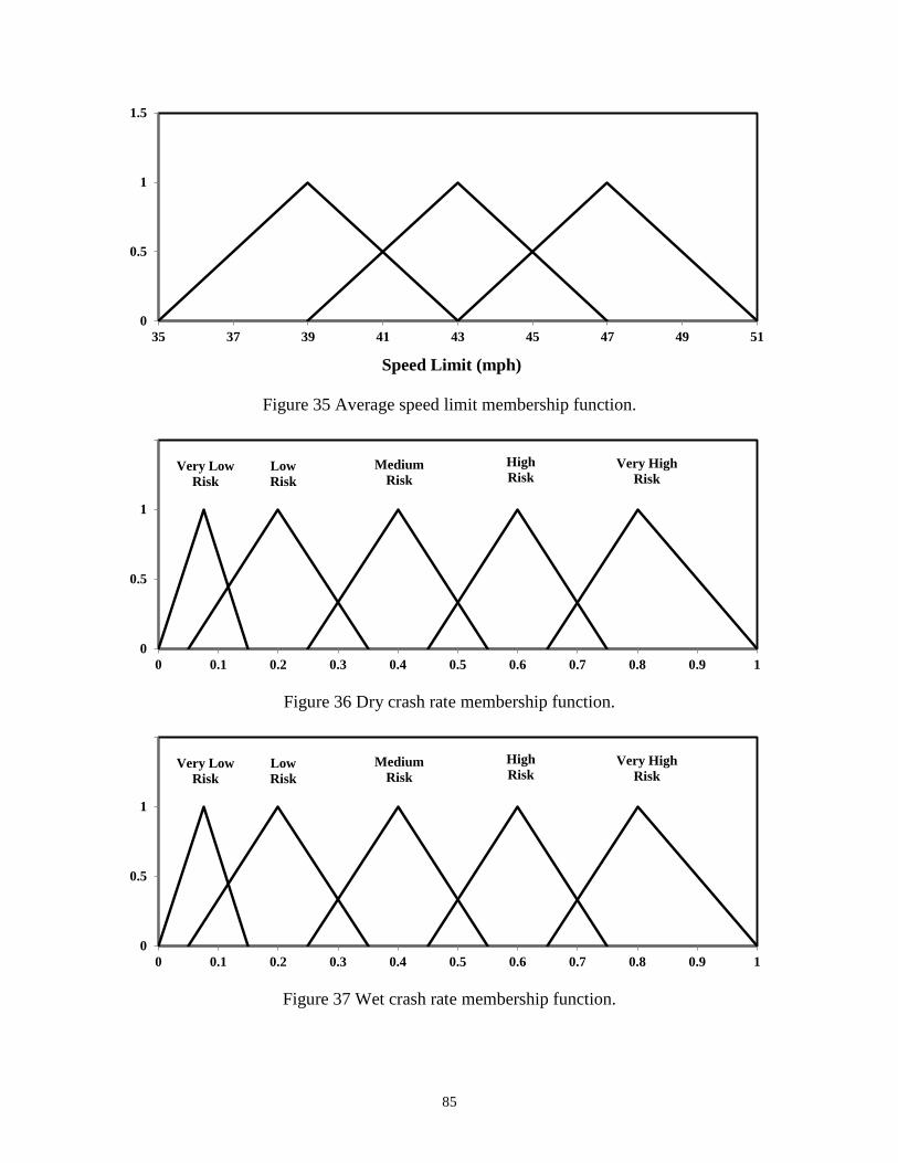
0
0.5
1
1.5
35 37 39 41 43 45 47 49 51
Speed Limit (mph)
Figure 35 Average speed limit membership function.
0
0.5
1
1.5
0 0.1 0.2 0.3 0.4 0.5 0.6 0.7 0.8 0.9 1
Very Low Risk
Low Risk
Medium Risk
HighRisk
Very HighRisk
Figure 36 Dry crash rate membership function.
0
0.5
1
1.5
0 0.1 0.2 0.3 0.4 0.5 0.6 0.7 0.8 0.9 1
Very Low Risk
Low Risk
Medium Risk
HighRisk
Very HighRisk
Figure 37 Wet crash rate membership function.
85

Fuzzy Rules
Once the membership functions are defined, the fuzzified inputs are combined according to
fuzzy rules. Mamdani fuzzy rules are if-then in nature (i.e., IF functional classification is urban
principal arterial AND friction is very low AND speed limit is high AND AADT is high THEN
dry crash rate is high and wet crash rate is high). The rules are then combined to generate the
output distribution. In the Mamdani interface, ‘max’ and ‘min’ operators are used to aggregate
the fuzzy rules. The Mamdani fuzzy logic operator can be mathematically expressed as follows
(Youssefi et al. 2011):
)()())(),(( xxyxf BABA mmmm ∧= (28)
Where µA(x) indicates the membership function of x.
The outputs can then be defuzzified to a ‘crisp’ value using the centroid method (Lee 1990):
dxxxdxxx
i
i
)()(*
mm∫∫
= (29)
Where,
x* is the defuzzified output
µi(x) is the aggregated membership function, and
x is the output variable.
The Graphical User Interface (GUI) of MATLAB software package was used to develop
the Mamdani fuzzy inference system. The inputs to the model included friction, AADT, and
speed limit. The outputs are dry and wet condition crash rates. The centroid method was used to
defuzzify the outputs.
Mamdani fuzzy rules are provided in Table 9. The rules were developed by observing
trends in the database. The mean squared error (MSE) between predicted and actual crash rates
was calculated to estimate the accuracy of the model. A value closer to zero is desirable as it
indicates smaller random error in the model. The MSE between observed and predicted for both
dry and wet crash rates was approximately 0.01.
86

Table 9 Mamdani Fuzzy Rules
Friction AADT Speed Limit Dry Crash Rate Wet Crash Rate very low medium medium very high very high low medium high very high very high low medium low very high high low high high high high medium high high medium medium high high high low very low very high low high low medium very high medium high low very low very high high high very low very low
Sugeno Fuzzy Inference System
The Sugeno fuzzy inference system is similar to Mamdani’s system in several ways. Both
systems fuzzify the inputs in the same way and apply the same fuzzy operator. The main
difference is that Sugeno output functions are either linear or constant. Sugeno fuzzy rules have
the following form (Sugeno 1985):
If (30) Input 1 = x
and Input 2 = y
then z = ax + by + c
Where the output z will be constant if a = b = 0. The outputs will be assigned a weight (wi)
based on their strength. Unlike the Madani system, the Sugeno system doesn’t use
defuzzification to generate outputs. Instead, the weighted average of rule outputs is used to
calculate the crisp output (Sugeno 1985):
∑
∑
=
== n
ii
n
iii
w
zw
1
1η (31)
Where, η is the final crisp output, and
87
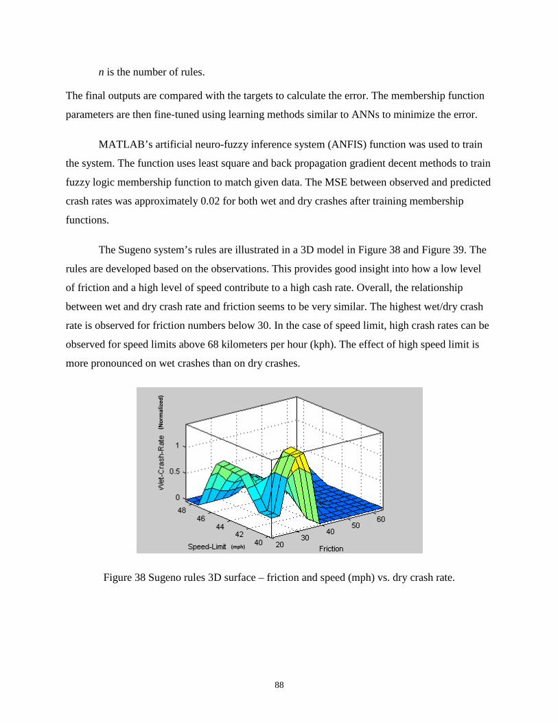
n is the number of rules.
The final outputs are compared with the targets to calculate the error. The membership function
parameters are then fine-tuned using learning methods similar to ANNs to minimize the error.
MATLAB’s artificial neuro-fuzzy inference system (ANFIS) function was used to train
the system. The function uses least square and back propagation gradient decent methods to train
fuzzy logic membership function to match given data. The MSE between observed and predicted
crash rates was approximately 0.02 for both wet and dry crashes after training membership
functions.
The Sugeno system’s rules are illustrated in a 3D model in Figure 38 and Figure 39. The
rules are developed based on the observations. This provides good insight into how a low level
of friction and a high level of speed contribute to a high cash rate. Overall, the relationship
between wet and dry crash rate and friction seems to be very similar. The highest wet/dry crash
rate is observed for friction numbers below 30. In the case of speed limit, high crash rates can be
observed for speed limits above 68 kilometers per hour (kph). The effect of high speed limit is
more pronounced on wet crashes than on dry crashes.
(mph)
(Nor
mal
ized
)
Figure 38 Sugeno rules 3D surface – friction and speed (mph) vs. dry crash rate.
88
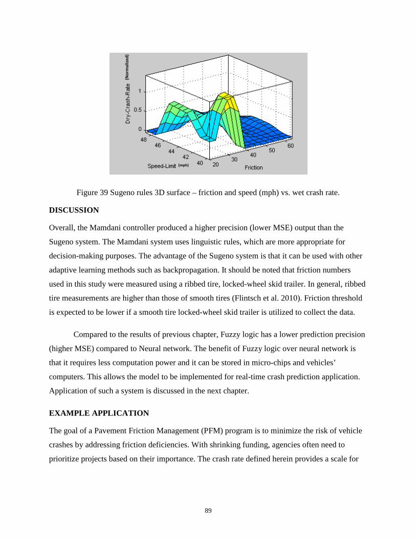
(mph)
(Nor
mal
ized
)
Figure 39 Sugeno rules 3D surface – friction and speed (mph) vs. wet crash rate.
DISCUSSION
Overall, the Mamdani controller produced a higher precision (lower MSE) output than the
Sugeno system. The Mamdani system uses linguistic rules, which are more appropriate for
decision-making purposes. The advantage of the Sugeno system is that it can be used with other
adaptive learning methods such as backpropagation. It should be noted that friction numbers
used in this study were measured using a ribbed tire, locked-wheel skid trailer. In general, ribbed
tire measurements are higher than those of smooth tires (Flintsch et al. 2010). Friction threshold
is expected to be lower if a smooth tire locked-wheel skid trailer is utilized to collect the data.
Compared to the results of previous chapter, Fuzzy logic has a lower prediction precision
(higher MSE) compared to Neural network. The benefit of Fuzzy logic over neural network is
that it requires less computation power and it can be stored in micro-chips and vehicles’
computers. This allows the model to be implemented for real-time crash prediction application.
Application of such a system is discussed in the next chapter.
EXAMPLE APPLICATION
The goal of a Pavement Friction Management (PFM) program is to minimize the risk of vehicle
crashes by addressing friction deficiencies. With shrinking funding, agencies often need to
prioritize projects based on their importance. The crash rate defined herein provides a scale for
89

highway agencies to use for prioritizing safety projects based on crash risk so they can advance a
resurfacing project if the site is already in the queue for resurfacing and the crash risk is high.
To better understand the relationship between friction and crash rate, a sensitivity
analysis for both systems was performed by setting the speed limit and ADDT to average (72
kph and 15,000 vph respectively) and changing the friction level (Figure 40). Both wet and dry
crash rates decreased as friction increased. This is in agreement with previous findings that
friction affects crash rate in both wet and dry conditions (Najafi et al. 2015).
The relationship between friction and crash rate can also be used to define the desirable
friction threshold. For instance, a friction level that induces high crash risk—at any given traffic
level and speed limit—can be selected as the investigatory threshold. An agency can define
multiple levels of friction and crash risk based on their internal policies. This will allow them to
narrow sections of roadway designated for improvement into smaller sets, and gives them the
flexibility to prioritize the sections based on available funds. More sections can be added to the
list as funding becomes available.
90

0
0.1
0.2
0.3
0.4
0.5
0.6
0.7
0.8
0.9
1
20 22 24 26 28 30 32 34 36 38 40 42 44 46 48 50 52 54 56 58 60 62 64
Cra
sh R
ate
Friction
Predicted Dry Crash Rate-Sugeno Predicted Wet Crash Rate-Sugeno
Predicted Dry Crash Rate-Mamdani Predicted Dry Crash Rate-Mamdani
High Risk
Investigatory Level
Figure 40 Sensitivity analysis.
FINDINGS AND CONCLUSIONS
This paper proposed a fuzzy logic approach for PFM. Following are the main findings and
conclusions of the study:
• The fuzzy logic interface system is a reliable tool for the PFM decision-making process.
The system can be easily modified based on agency needs. The model uses linguistic and
human like rules and is easy for practitioners and highway engineers to understand.
• Crash risk can be predicted based on friction, traffic, and speed limit using both Mamdani
and Sugeno controllers. The Mamdani controller produced a higher precision (lower
MSE) prediction than the Sugeno system. The advantage of the Sugeno system is that it
can be used with other adaptive learning methods such as backpropagation. The
91

Mamdani system uses linguistic rules, which are more appropriate for decision-making
purposes.
• The rate of both wet and dry condition crashes increases as the roadway friction
decreases. The highest wet/dry crash rate was observed for friction numbers below 30
and speed limits above 68 kph. Using both wet and dry condition crashes in PFM studies
is suggested.
• The investigatory threshold level of friction can be defined based on the crash risk.
Agencies can modify the level based on available funding. This allows highway agencies
to prioritize resources based on safety needs so they can advance a resurfacing project if
the site is already in the queue for resurfacing and the crash risk is high.
ACKNOWLEDGEMENT
The authors would like to acknowledge the New Jersey Department of Transportation and, in
particular, Susan Gresavage for their contribution and support in providing the data for this
study.
REFERENCES
Chen, C. (2007). “Soft Computing-based Life-Cycle Cost Analysis Tools for Transportation
Infrastructure Management." Virginia Polytechnic Institute and State University.
Chassiakos A.K. (2006), “A Fuzzy-based system for maintenance planning of road pavements”,
Proceeding of the 10th WSEAS International conference on computer, Vouliagmeni, Athens,
Greece, pp535-540, July 13-15.
Dieckmann, T. (1992). "Assessment of Road Grip byWay of Measured Wheel Variables."
Proceedings of FISITA ’92 Congress, London, GB, 2:75–81, June 7–11. ‘‘Safety the Vehicle and
the Road.’’.
Erdogan, G., L. Alexander, et al. (2009). "Friction coefficient measurement for autonomous
winter road maintenance." Vehicle System Dynamics 47(4): 497-512.
92
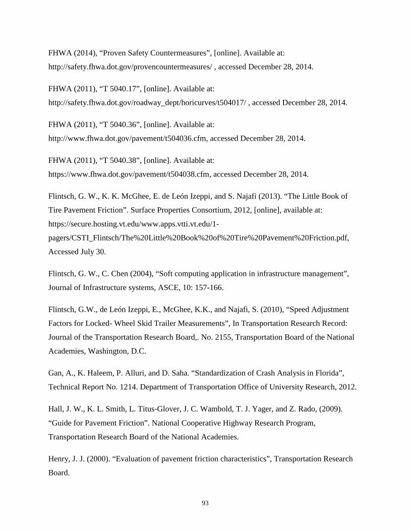
FHWA (2014), “Proven Safety Countermeasures”, [online]. Available at:
http://safety.fhwa.dot.gov/provencountermeasures/ , accessed December 28, 2014.
FHWA (2011), “T 5040.17”, [online]. Available at:
http://safety.fhwa.dot.gov/roadway_dept/horicurves/t504017/ , accessed December 28, 2014.
FHWA (2011), “T 5040.36”, [online]. Available at:
http://www.fhwa.dot.gov/pavement/t504036.cfm, accessed December 28, 2014.
FHWA (2011), “T 5040.38”, [online]. Available at:
https://www.fhwa.dot.gov/pavement/t504038.cfm, accessed December 28, 2014.
Flintsch, G. W., K. K. McGhee, E. de León Izeppi, and S. Najafi (2013). “The Little Book of
Tire Pavement Friction”. Surface Properties Consortium, 2012, [online], available at:
https://secure.hosting.vt.edu/www.apps.vtti.vt.edu/1-
pagers/CSTI_Flintsch/The%20Little%20Book%20of%20Tire%20Pavement%20Friction.pdf,
Accessed July 30.
Flintsch, G. W., C. Chen (2004), “Soft computing application in infrastructure management”,
Journal of Infrastructure systems, ASCE, 10: 157-166.
Flintsch, G.W., de León Izeppi, E., McGhee, K.K., and Najafi, S. (2010), “Speed Adjustment
Factors for Locked- Wheel Skid Trailer Measurements”, In Transportation Research Record:
Journal of the Transportation Research Board,. No. 2155, Transportation Board of the National
Academies, Washington, D.C.
Gan, A., K. Haleem, P. Alluri, and D. Saha. “Standardization of Crash Analysis in Florida”,
Technical Report No. 1214. Department of Transportation Office of University Research, 2012.
Hall, J. W., K. L. Smith, L. Titus‐Glover, J. C. Wambold, T. J. Yager, and Z. Rado, (2009).
“Guide for Pavement Friction”. National Cooperative Highway Research Program,
Transportation Research Board of the National Academies.
Henry, J. J. (2000). “Evaluation of pavement friction characteristics”, Transportation Research
Board.
93

Hwang, W. and B.-S. Song (2000). “Road condition monitoring system using tire-road friction
estimation”. Proceedings of AVEC 2000 5th International Symposium of Advanced Vehicle
Control.
Ivey, D. L., L. I. Griffin III, J. R. Lock, and D. L. Bullard. “Texas Skid Initiated Accident
Reduction Program”, Final Report, Research Report 910-1F, TTI: 2-18-89/910, TX-92/910-1F.
Texas Department of Transportation, Austin, Texas, 1992.
Kou, Kuang-Yang (2005), “The modeling of wet-pavement related crashes by using fuzzy
logic”, 2005 IEEE International Conference on Systems, Man and Cybernetics.
Lee, C. (1990). ‘‘Fuzzy logic in control systems: fuzzy logic controller, Parts I and II’’, IEEE
Trans. Syst., Man, Cybern., vol. 20, pp. 404–435.
Mamdani, E.H. and S. Assilian (1975), "An experiment in linguistic synthesis with a fuzzy logic
controller," International Journal of Man-Machine Studies, Vol. 7, No. 1, pp. 1-13.
Najafi, S., Flintsch, G.W., de León Izeppi, E., McGhee, K.K., and Katicha S. (2011),
“Implementation of Crosscorrelation to Compare Continuous Friction Measuring Equipment
(CFME)”, CD-ROM. Transportation Research Board of the National Academies, Washington,
D.C.
Najafi, S., Flintsch, G.W., Medina, A. (2014), “Case Study on the Evaluation of the Effect of
Friction on the Rate of Fatal and Injury Causing Car Crashes”, 93rd Annual Meeting of
Transportation Research Board of the National Academies, CD-ROM. Washington, D.C.
Najafi, S., G. W. Flintsch, and A. Medina, (2015). “Linking roadway crashes and tire–pavement
friction: a case study”. International Journal of Pavement Engineering, DOI:
10.1080/10298436.2015.1039005.
NOAA, “National Oceanic and Atmospheric Administration” [online]. Available at:
www.ncdc.noaa.gov/cdo-web/datasets, accessed August 30, 2015.
Richard S., “Development of fiction improvement policies and guidelines for the Maryland state
highway administration” [online], available at:
94
http://www.roads.maryland.gov/OPR_Research/MD-09-SP708B4F-Development-of-Friction-
Improvement-Policies-and-Guidelines_Report.pdf accessed December 28, 2014.
Sandra A.K.,Vinayaka Rao V.R.,Raju K.S.,Sarkar A.K. (2010),“Priotization of Pavement
Stretches using Fuzzy MCDM Approach - A Case Study‟. [online], available at:
http://www.cs.armstrong.edu/wsc11/pdf/pap154s2-file1.pdf accessed December 28, 2014.
Suman S.K., S.Sinha, (2012). “Pavement Maintenance Treatment Selection Using Fuzzy Logic Inference
System”. International Journal of Engineering and Innovative Technology (IJEIT). ISSN: 2277-3754.
Volume 2, Issue 6, December 2012.
Sugeno, M. (1985). ‘‘An introductory survey of fuzzy control,’’ Inf. Sci., vol. 36, pp. 59–83.
Xiao, J., B. T. Kulakowski, and M. El-Gindy (2000). “Prediction of Risk of Wet-Pavement
Accidents: Fuzzy Logic Model”, Transportation Research Record 1717, Transportation Research
Board, Washington, D.C.
Youssefi H., V. S. Nahaei, J. Nematian (2011), “A New Method for Modeling System Dynamics
by Fuzzy Logic: Modeling of Research and Development in the National System of Innovation”,
the Journal of Mathematics and Computer Science Vol .2 No.1, 88-99.
Zadeh L. A. (1965), “Fuzzy sets.” Inf. Control, 8 338-353.
95
CHAPTER 5 – APPLICATION OF FUZZY LOGIC INFERENCE SYSTEM
IN A REAL-TIME SLIPPERY ROAD WARNING SYSTEM -A PROOF OF
CONCEPT STUDY
INTRODUCTION
Recently, the USDOT has begun promoting the concept of connected vehicles to improve the
safety of, and ease of mobility throughout, the transportation infrastructure system. Connected
vehicles can increase drivers’ awareness and reduce the risk of crashes through vehicle-to-
vehicle (V2V) and vehicle-to-infrastructure (V2I) data transmission. This application will inform
drivers of roadway hazards in real-time. According to the USDOT, ‘combined V2V and V2I
systems potentially address about 81 percent of all-vehicle target crashes; 83 percent of all light-
vehicle target crashes; and 72 percent of all heavy-truck target crashes annually’ (USDOT 2015).
The USDOT has also performed a safety pilot study to collect V2V and V2I data under
real-world conditions. The safety applications evaluated in the safety pilot include the following:
Blind Spot Warning/Lane Change Warning (warns drivers if there is a car in the blind spot
during an attempted lane change), Forward Collision Warning (warns drivers when a vehicle in
their path is stopped or is traveling slower and they fail to brake), Electronic Emergency Brake
Lights (notifies the driver when a vehicle ahead of them is braking hard), Intersection Movement
Assist (warns the driver if it is unsafe to enter an intersection), Do Not Pass Warning (warns
drivers if they attempt a lane change when there is another vehicle coming from the opposite
direction in the passing zone), Control Loss Warning (warns the driver if another adjacent
vehicle has lost control) (USDOT 2015).
‘Slippery when wet’ and ‘Watch for ICE’ signs have been implemented for years across
US highways and other parts of the world. A real-time slippery road warning system can provide
immediate alerts to drivers for potentially hazardous locations. The information can also be
transmitted to a central traffic control center to be used in snow and ice removal operations or to
plan maintenance activities to correct friction deficiencies. The fuzzy system discussed in the
previous chapter is capable of predicting the crash risk based on available friction and speed
limit. Most modern Global Positioning Systems (GPS) report the speed limit and traffic volume
96

information in real-time. This means the model can be used in real-time if friction can be
measured simultaneously.
REAL-TIME FRICTION ESTIMATION
Due to the importance of tire-pavement friction in vehicle dynamics and stability control,
several researchers have investigated various methods of estimating the tire-pavement friction in
real time. (Erdogan et al. 2009). Real-time friction estimation can be separated into two
categories: 1) sensor-based estimation, and 2) vehicle dynamic-based estimation (Rajamani et al.
2010). The main drawback of sensor-based tire-pavement friction estimation is the cost
associated with acquiring the sensors. Installing the sensors in the vehicle or tire carcass can also
raise liability issues. Some sensor lasers also have limited application during wet weather
conditions. For these reasons, the sensor-based method will not be further investigated for this
study. In the vehicle dynamic control-based approach, tire-pavement friction is estimated based
on the vehicle’s motion. This method uses the measurements from the sensors already installed
in the vehicle, which gives it an advantage over the sensor-based approach, which requires the
installation of additional sensors.
As the tire rolls freely on the pavement surface, longitudinal frictional forces are
generated at the tire and pavement interface. The relative speed between the tire circumference
and the pavement surface is very low during the free rolling (no braking) condition. Applying a
constant brake to the tire will increase the slip speed to the potential maximum equivalent of the
vehicle speed. The slip ratio (Sr) can be calculated from the vehicle’s directional speed (V), the
wheel’s angular velocity (ω ) and the wheel-rolling radius (R):
VRVSr
ω−= (32)
Where slip ratio is zero under normal driving condition ( RV ω= ) and it is 1 when the wheel is
fully locked ( 0=ω ).
The relationship between tire friction force and slip ratio for various road surfaces with
different friction levels is presented in Figure 41. For small slip ratios, the tire friction force is
‘proportional’ to slip ratio (Rajamani et al. 2010). The coefficient of friction can be determined
97
based on the slope at the low slip region; this is commonly known as slip-slope (Rajamani et al.
2010). As illustrated by the figure, the slip-slope for roads with higher friction is larger. Some
references argue that tire properties influence the ‘shape’ of the low slip region more than the
road surface properties (Henry 2000; Uchanski et al. 2003). However, studies show that for slip
ratios greater than 0.005, the slip-slope method can reliably estimate the coefficient of friction
(Rajamani et al. 2010). Several studies (Dieckmann 1992; Germann et al. 1994; Gustafsson
1997; Yi et al. 1999; Hwang and Song 2000) have previously used this method to estimate the
tire-pavement friction.
Wet AsphaltHard SnowIce
Dry Concrete
0 0.05 0.1 0.15-0.05-0.1-0.15
0
0.40.2
0.60.81.0
-0.2-0.4-0.6-0.8-1.0
Slip Ratio
Tire
Fri
ctio
n Fo
rce
Figure 41 Tire Friction Force versus slip ratio (after Rajamani et al. (2010)).
Slip-slope based Friction Estimation
The inputs to the slip-slope based friction estimation method include normalized longitudinal tire
force and slip ratio. The normalized longitudinal tire force (also known as normalized traction
force) can be determined by dividing the traction force (Ff) by the normal force on the drive
wheel (N). For a vehicle in longitudinal motion, this relationship can be expressed as follows:
rf KS
NF
= (33)
98
Where, Ff = Longitudinal traction force
N = Normal tire force, and K = Slip-slope.
The total longitudinal traction forces can be estimated using Newton’s second law of motion
(∑Fx = max). Where m is the mass of the vehicle and ax is the longitudinal acceleration or
deceleration. This relationship can be formulated as follows (Rajamani et al. 2010):
2VDFamF arxf ++= , for acceleration (34)
2VDFamF arxf −−= , for deceleration (35)
And,
mgCF rollr = (36)
ACVD da2
21 ξ= (37)
Where, Fr = Rolling resistance force
Da = Aerodynamic drag force Croll = Rolling resistance coefficient ξ = Air density V = Speed Cd = Aerodynamic drag coefficient A = Frontal area of the vehicle
The longitudinal acceleration/deceleration (ax) can be measured using accelerometers.
The vehicle’s directional speed can be measured with a GPS. The angular speed of the wheels
can be obtained from the antilock brake system (ABS). The normal tire force (N) can be
calculated using a simple static force equilibrium model of the vehicle, assuming that the
vehicle’s weight is known. More details about the procedure can be found in Rajamani et al.
(2010). Assuming that the vehicle is all-wheel-drive, we will have:
rearfrontrearfrontotal rrearrearrfrontfrontfff SNKSNKFFF +=+= (38)
For two-wheel drive vehicles, Kfront or Krear is zero. The ratio between Kfront and Krear is known to
be constant and depends on tire properties and number of tires for front and rear axles (Rajamani
et al. 2010):
99
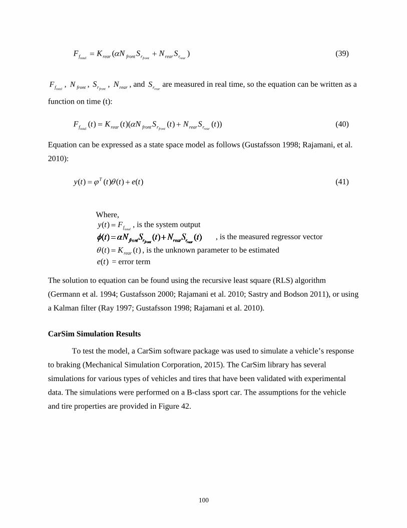
)(rearfronttotal rrearrfrontrearf SNSNKF += α (39)
totalfF , frontN , frontrS , rearN , and
rearrS are measured in real time, so the equation can be written as a
function on time (t):
))()()(()( tSNtSNtKtFrearfronttotal rrearrfrontrearf += α (40)
Equation can be expressed as a state space model as follows (Gustafsson 1998; Rajamani, et al.
2010):
)()()()( tettty T += θϕ (41)
Where, totalfFty =)( , is the system output
, is the measured regressor vector
)()( tKt rear=θ , is the unknown parameter to be estimated )(te = error term
The solution to equation can be found using the recursive least square (RLS) algorithm
(Germann et al. 1994; Gustafsson 2000; Rajamani et al. 2010; Sastry and Bodson 2011), or using
a Kalman filter (Ray 1997; Gustafsson 1998; Rajamani et al. 2010).
CarSim Simulation Results
To test the model, a CarSim software package was used to simulate a vehicle’s response
to braking (Mechanical Simulation Corporation, 2015). The CarSim library has several
simulations for various types of vehicles and tires that have been validated with experimental
data. The simulations were performed on a B-class sport car. The assumptions for the vehicle
and tire properties are provided in Figure 42.
100

Figure 42 B-Class Sport Car (CarSim, (2015)).
The vehicle and tire properties were kept constant and the surface friction was changed to
simulate the braking response. Two surfaces were considered: one with very low friction
(friction coefficient = 0.2) and one with high friction (friction coefficient = 0.8). Longitudinal
and angular velocity, tire longitudinal force, and slip ratio were simulated in real-time for both
surfaces. The simulated data were then used to predict the real-time friction using the Kalman
filter in the MATLAB software package. For brevity, the procedure for the Kalman filtering
process is not provided here. Figure 43 and Figure 44 illustrate the MATLAB’s estimated
friction force versus CarSim’s simulation (real) data. As the figure illustrates, the estimated
friction is almost identical to real friction in the low slip region. As expected, the slip-slop for the
slippery road is lower than for the high friction surface (7% versus 17% respectively).
0 0.2 0.4 0.6 0.8 10
0.2
0.4
0.6
0.8
1
Slip Ratio
realestimated
Fric
tion
Coe
ffici
ent
Figure 43 Friction vs. slip ratio estimation – high friction surface (friction coefficient = 0.8).
101
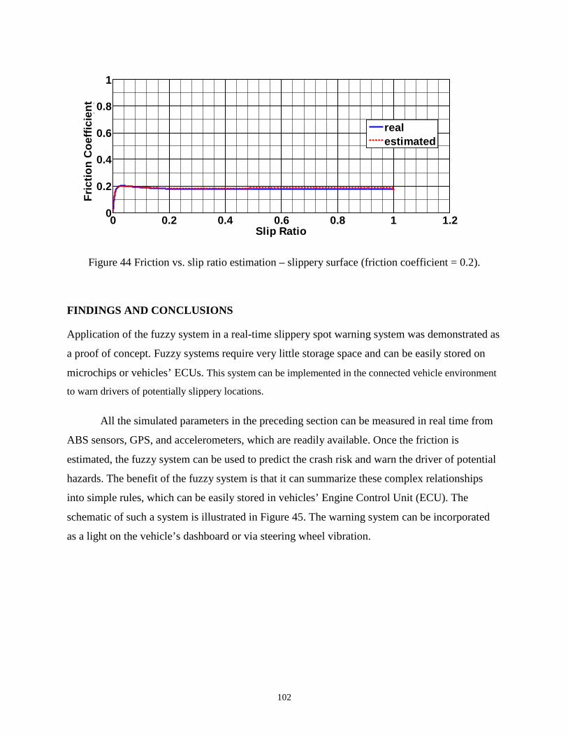
0 0.2 0.4 0.6 0.8 1 1.20
0.2
0.4
0.6
0.8
1
Slip Ratio
(
)
realestimated
Fric
tion
Coe
ffici
ent
Figure 44 Friction vs. slip ratio estimation – slippery surface (friction coefficient = 0.2).
FINDINGS AND CONCLUSIONS
Application of the fuzzy system in a real-time slippery spot warning system was demonstrated as
a proof of concept. Fuzzy systems require very little storage space and can be easily stored on
microchips or vehicles’ ECUs. This system can be implemented in the connected vehicle environment
to warn drivers of potentially slippery locations.
All the simulated parameters in the preceding section can be measured in real time from
ABS sensors, GPS, and accelerometers, which are readily available. Once the friction is
estimated, the fuzzy system can be used to predict the crash risk and warn the driver of potential
hazards. The benefit of the fuzzy system is that it can summarize these complex relationships
into simple rules, which can be easily stored in vehicles’ Engine Control Unit (ECU). The
schematic of such a system is illustrated in Figure 45. The warning system can be incorporated
as a light on the vehicle’s dashboard or via steering wheel vibration.
102
ω
GPS
N
Ff
Accelerometer
ax
Fr
Da
V
K (Friction)
Speed LimitFuzzy Logic Controller
Crash Risk
Traffic
Figure 45 Fuzzy controller real-time slippery road warning system framework.
REFERENCES
Germann, S., M. Wurtenberger, et al. (1994). “Monitoring of the friction coefficient between tyre
and road surface”. Control Applications, 1994., Proceedings of the Third IEEE Conference on,
IEEE.
Gustafsson, F. (1997). "Slip-based tire-road friction estimation." Automatica 33(6): 1087-1099.
Gustafsson, F. (1998). "Monitoring tire-road friction using the wheel slip." Control Systems,
IEEE 18(4): 42-49.
Gustafsson, F. (2000). “Adaptive filtering and change detection”, Wiley New York.
103

Henry, J. J. (2000). “Evaluation of pavement friction characteristics”, Transportation Research
Board.
Rajamani, R., N. Piyabongkarn, et al. (2010). "Tire-road friction-coefficient estimation." Control
Systems, IEEE 30(4): 54-69.
Ray, L. R. (1997). "Nonlinear tire force estimation and road friction identification: simulation
and experiments." Automatica 33(10): 1819-1833.
Sastry, S. and M. Bodson (2011). “Adaptive control: stability, convergence and robustness”,
Courier Dover Publications.
Uchanski, M., K. Hedrick, et al. (2003). "Estimation of the maximum tire-road friction
coefficient." Journal of dynamic systems, measurement, and control 125(4): 607-617.
USDOT (2015), “Connected Vehicle Research in the United States”. [online], available at:
http://www.its.dot.gov/connected_vehicle/connected_vehicle_research.htm. accessed September
12, 2015.
Yi, K., K. Hedrick, et al. (1999). "Estimation of tire-road friction using observer based
identifiers." Vehicle System Dynamics 31(4): 233-261.
104
CHAPTER 6 - OPTIMIZING PAVEMENT SURFACE
CHARACTERISTICS THROUGH DIAMOND GRINDING AND
GROOVING TECHNIQUE – A CASE STUDY AT THE VIRGINIA SMART
ROAD7
ABSTRACT
Providing a smooth, safe, and quite riding surface is an ultimate goal for pavement engineers. To
achieve this goal a balance between high friction level and low roughness and noise level needs
to be made. Diamond grinding and grooving is one of the techniques that can be used to improve
pavement smoothness while increasing the drivers’ safety by improving the frictional properties
of the riding surface. This paper evaluates the effect of diamond grinding and grooving on
various surface characteristics of concrete pavements. Measurements for texture, friction, and
smoothness have been collected on two continuously reinforced concrete pavements at the
Virginia Smart Road. One of the sections was diamond grinded and longitudinally grooved while
the other section was transversely tinned.
The results of the study show that diamond grinding and grooving increases the surface
macrotexture which helps in improving the surface friction. Friction was measured using both
smooth tire and ribbed tire locked wheel trailers. Smooth tire measurements confirmed that
diamond grinding and grooving increases the friction, however, ribbed tire skid trailer did not
show this effect. Several single spot laser profilers and a SURPRO reference profiler were used
to measure the surface smoothness before and after grinding and grooving. Longitudinal
grooving made the single spot laser profilers incapable of measuring the correct road profile.
Power Spectral Density (PSD) analysis revealed that longitudinal grooving introduces artificial
wavelengths in the profiles collected by single spot laser profilers. According to the reference
profiler results, diamond grinding and grooving improved the concrete surface smoothness.
7 This manuscript IJP-P13-02 has been accepted for publication in the International Journal of Pavements and it is in pre-print. Co-authors include: Sameer Shetty, Gerardo Flintsch, and Larry Scofield.
105
INTRODUCTION
Diamond grooving is a technique that is used in order to improve the frictional properties of the
pavement surfaces (Martinez 1997). Most of the developments in diamond grinding and
grooving occurred in the state of California in the early 1960s (Scofield 2012). The main purpose
of this practice was to restore the skid resistance of old concrete pavements (Scofield 2012).
Friction of the pavement surface is an important factor contributing to road safety. Each year
many people around the United States (U.S.) lose their lives as a result of car crashes. Due to the
importance of friction in reducing the rate of car crashes, the Federal Highway administration
(FHWA) has started to implement new policies that require the state Departments of
Transportation (DOTs) to implement highway safety programs. Diamond grinding and grooving
can be a good option for state DOTs to restore the frictional properties of old concrete pavement
in their road network.
Along with friction, roadway smoothness is an important surface characteristic that
affects the ride quality, operation cost, and vehicle dynamics. Currently, most state DOTs use
laser inertial profilers to measure the road roughness. Measurements are summarized using the
International Roughness Index (IRI) which was developed by National Cooperative Highway
Research Program (NCHRP) and World Bank. Smoothness measurements can be used to
evaluate the ride quality of existing road networks or as a quality check for newly constructed
pavements. Due to the importance of ride quality to the road users, highway agencies have
implemented smoothness based specification for newly constructed as well as rehabilitated
pavements. The smoothness specification identifies an acceptable range of smoothness that the
contractor must achieve to obtain full payment. All highway agencies assess penalties if the
achieved smoothness is less than specified, while many highway agencies give bonuses to
contractors who achieve a smoothness level that is higher than the specified level. Diamond
grinding and grooving is one of the methods which can be used to improve the smoothness of
both old and new pavement surfaces.
106
OBJECTIVE
The objective of this paper is to evaluate the effect of diamond grinding and grooving on surface
characteristics of concrete pavement. In particular, the paper investigates the changes in
macrotexture, friction, and smoothness of a concrete pavement subjected to diamond grinding
and longitudinal grooving. Measurements for this study were collected at the Virginia Smart
Road during the 2010 and 2011 annual equipment round up (Rodeo 2010 & 2011).
BACKGROUND
One of the main goals of pavement engineers is to provide a smooth, safe and quiet riding
surface for road users. In order to achieve this goal, a balance should be made between high level
of friction and low level of smoothness and noise. Both, friction and noise are affected by
pavement macrotexture. High macrotexture improves road safety by increasing the draining
properties of the road surface. It also helps reducing the tire-pavement noise level (Karamihas et
al. 2004). Several devices are available for measuring friction. Most state DOTs in the U.S.
currently use the locked wheel friction trailer. The trailer can measure the longitudinal friction in
fully locked condition (100% slip). Because Most of skidding accidents happen during wet
weather condition due to friction deficiencies (Wambold et al. 1986), the device is equipped with
a water distribution system that sprays water in front of the tire during the test so it can measure
the wet friction.
From the functional point of view, smoothness is an important roadway performance
indicator since road users primarily judge the quality of a road based on its roughness and/or ride
quality. According to the national highway user survey (1995 and 2000) (Perera et al. 2002),
pavement roughness/ride quality was rated as one of the top three principal measures of public
satisfaction within a road system. Earlier studies (Karamihas et al. 1999) have shown that rough
roads lead to user discomfort, increased travel time due to lower speeds and higher vehicle
operating cost. As such, road roughness is now widely recognized as one of the principal
measures of pavement performance. Different techniques are available for measuring road
smoothness, most of which measure the vertical deviations of the road surface along a
longitudinal line of travel in a wheel path, known as a profile (Sayers et al. 1998). Traditionally,
the profilograph has been used to measure the smoothness of road pavements. The profile
107
recorded by the profilograph is analyzed to determine the profile index (PI), which is the
smoothness index that is used to judge the ride quality of the pavement. However, several
inherent weaknesses were observed in the profilograph and PI for judging the ride quality of a
pavement, and hence many state highway agencies have instead adopted the International
Roughness Index (IRI) as the ride quality parameter for assessing the smoothness of
new/rehabilitated pavements. Inertial profilers are used to obtain profile data to compute the IRI
(Shahin et al. 2005).
Diamond grinding and grooving is one of the rehabilitation practices that can be used on
old concrete pavements in order to make the surface smoother. The method uses diamond
infused steel cutting blades for grinding and grooving concrete pavement. For grinding, the
blades are spaced close together so that they can cut the pavement’s unevenness (megatexture)
and leave a rough pavement surface (high microtexture). For grinding, the blades are further
spaced out so they create channels on the pavement surface (high macrotexture). Diamond
grooving is mainly used for new concrete pavement to texture the pavement which increases the
friction by improving water drainage (Wulf et al. 2008).
Several studies have recently been performed to investigate the effect of diamond
grinding and grooving on the noise level of pavements. Research has shown that longitudinal
diamond grinding is one of the quietest types of surface finishing for concrete pavement (Dare et
al. 2011). In the U.S. most of the grooving on highways are longitudinal while transverse
grooving is more common for runways (Martinez 1977).
TEST PROCEDURE
The data for this study was collected at the Virginia Smart Road during the annual equipment
roundup (Rodeo) in two consecutive years; 2010 and 2011. The Virginia Smart Road provides a
3.2 km (2 mi) controlled test track available for transportation research. The road consists of two
lanes and it has various types of pavement surfaces. Each year several sate DOTs meet at the
Virginia Smart Road with the purpose of equipment comparison on the available surfaces. This
event is called the annual equipment Rodeo.
The road has three continuously reinforced concrete sections on both east-bound and
west-bound directions that are transversely tinned. These sections were originally built and
108

tinned in 1999, at the time when the Smart Road was constructed. In order to evaluate the effect
of diamond grinding and grooving on Portland Cement Concrete (PCC) pavements, one of the
sections located along the west-bound direction was ground and longitudinally grooved by
International Grooving and Grinding Association (IGGA) in January 2011. The procedure
included a Conventional Diamond Ground (CDG) followed by longitudinal grooving. Two
different groove spacing were used for each half of the lane; 13 mm (½ inch) along the left wheel
path and 19 mm (¾ inch) along the right wheel path (Roberts 2011). Figure 46 illustrates the
close up of grooving on the PCC section.
(a) PCC left wheel path, 13 mm (½ - inch) groove spacing.
(b) PCC right wheel path, 19 mm (¾ - inch) groove spacing.
Figure 46 Grooving on PCC section.
To evaluate the effect of diamond grinding and grooving on surface properties, several
measurements for texture, friction and smoothness were collected. The various tests used to
measure the surface properties are explained below.
Texture
Texture measurements were obtained using the ASTM E-2157 CTMeter. This static device has a
displacement sensor mounted on an arm at a radius of 142 mm (5.6 in) which rotates at a fixed
109

elevation from the surface. The device reports the Mean Profile Depth (MPD) and Root Mean
Square (RMS) according to ASTM E-2157 standard.
In order to determine the effect of diamond grinding and grooving on surface
macrotexture, measurements were collected on both tinned and grooved PCC. The tinned PCC
section is located along the east-bound lane while the grooved section is located along west-
bound lane. All the measurements for both sections were collected in the left wheel path and
overall three sets of measurements were obtained for each section. Table 10 shows the
macrotexture data for each test section.
Table 10 Macrotexture Measurements Using CT-Meter.
Section type # of Measurements Average MPD (mm)
Original tinned PCC 3 0.38
Diamond ground and grooved PCC 3 2.14
From the results of Table 10, it can be seen that diamond grinding and grooving has significantly
increased the macrotexture of the PCC pavement (higher MPD). This high macrotexture can
improve the skid resistance of the surface by reducing the effect of hydroplaning.
Friction
Friction measurements were obtained using two locked-wheel skid trailers. One of the locked
wheels used the ASTM E-524 smooth test tire while the other used the ASTM E-501 ribbed tire.
Five sets of measurements were obtained on both original tinned and grooved PCC at three
speeds; 40, 64, and 88 kph (25, 40, and 55 mph). All measurements were collect during Rodeo
2011. Figure 47 shows the layout of the test sections. The summary of the locked wheel
measurements is presented in Table 11.
110

Direction of the test
Direction of the test
Tinned PCC
Grooved PCC
N
19 mm (3/4-in)
13 mm (1/2-in)
Figure 47 Test sections layout.
Table 11 Summary of locked wheel skid trailer measurements Unit
# Test tire Test section Test speed (kph) # measurements Average skid number
1 Smooth
Original Tinned PCC
40 5 51.23
64 5 36.60
88 5 28.65
Ground and Grooved
PCC
40 5 58.90
64 5 56.07
88 5 44.97
2 Ribbed
Original Tinned PCC
40 5 67.77
64 5 64.07
88 5 53.10
Ground and Grooved
PCC
40 5 62.23
64 5 59.65
88 5 48.82
To evaluate the frictional properties of the tested surfaces, the correlation between skid number
and the test speed was calculated. In a previous study, the authors found a statistically significant
linear relationship between skid number and speed of the test vehicle for the range of speeds
from 32 to 96 kph (20 to 60 mph) (Flintsch et al. 2010).
111

Linear correlations were made for all measurements in Figure 48. Several observations
can be made. Smooth tires results show a significant increase in the skid numbers of the
concrete section subjected to diamond grinding and grooving. This agrees with the higher
measured macrotexture achieved on concrete after grinding and grooving. Another interesting
observation for smooth tires is the slope of the correlation line between skid number and speed
for the sections. This slope is less for ground and grooved PCC than it is for tinned PCC which
suggests that friction is less sensitive to the changes of speed for this section. At lower speeds
(40 kph) smooth tires measurements for both sections seem to be relatively close. However, at
high speeds the difference is much more evident (64 and 88 kph). In general, the effect of
hydroplaning is more pronounced at higher speeds; since the grooved section has a greater
macrotexture, it is less sensitive to hydroplaning and consequently provides increased friction at
high speeds.
Ribbed tires results, on the other hand, do not show a significant difference in the skid
values collected on the two test surfaces. The sensitivity of friction to speed is similar for both
tinned and ground and grooved test sections (parallel slopes). It is surprising that the ribbed tires
skid numbers are slightly higher for tinned PCC than the ground and grooved PCC. This seeming
paradox between smooth tire and ribbed tire results may be explained by sensitivity of the test
tire to the pavement surface texture and surface condition. Smooth tires are more sensitive to
macrotexture while ribbed tires are more sensitive to microtexture. It can therefore be postulated
that tinned PCC has a greater microtexture while ground and grooved concrete has a greater
macrotexture. Since the difference between ribbed tire measurements for the two types of PCC
surfaces is not significant, grooved concrete is a preferred choice for pavement surface as it
prevents hydroplaning at high speeds (i.e., it increases macrotexture). The lack of sensitivity of
ribbed tires to the effect of macrotexture has been cited by other researches (Wambold et al.
1986). There is evidence that pavement grooving significantly decrease the rate of wet-weather
accidents; however, ribbed tires fail to show this effect. For this reason some researchers believe
that smooth tires are a better choice for predicting skidding potentials (Wambold et al. 1986).
112
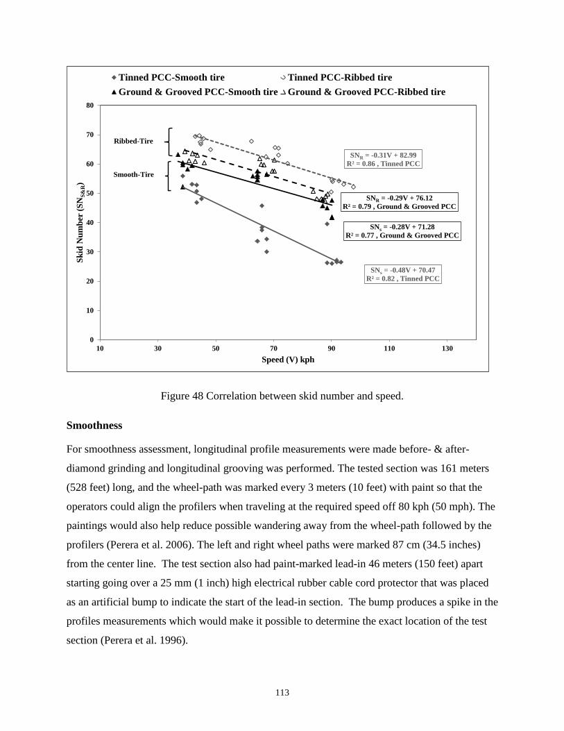
SNs = -0.48V + 70.47R² = 0.82 , Tinned PCC
SNR = -0.31V + 82.99R² = 0.86 , Tinned PCC
SNs = -0.28V + 71.28R² = 0.77 , Ground & Grooved PCC
SNR = -0.29V + 76.12R² = 0.79 , Ground & Grooved PCC
0
10
20
30
40
50
60
70
80
10 30 50 70 90 110 130
Skid
Num
ber
(SN
S&R)
Speed (V) kph
Tinned PCC-Smooth tire Tinned PCC-Ribbed tireGround & Grooved PCC-Smooth tire Ground & Grooved PCC-Ribbed tire
Ribbed-Tire
Smooth-Tire
Figure 48 Correlation between skid number and speed.
Smoothness
For smoothness assessment, longitudinal profile measurements were made before- & after-
diamond grinding and longitudinal grooving was performed. The tested section was 161 meters
(528 feet) long, and the wheel-path was marked every 3 meters (10 feet) with paint so that the
operators could align the profilers when traveling at the required speed off 80 kph (50 mph). The
paintings would also help reduce possible wandering away from the wheel-path followed by the
profilers (Perera et al. 2006). The left and right wheel paths were marked 87 cm (34.5 inches)
from the center line. The test section also had paint-marked lead-in 46 meters (150 feet) apart
starting going over a 25 mm (1 inch) high electrical rubber cable cord protector that was placed
as an artificial bump to indicate the start of the lead-in section. The bump produces a spike in the
profiles measurements which would make it possible to determine the exact location of the test
section (Perera et al. 1996).
113
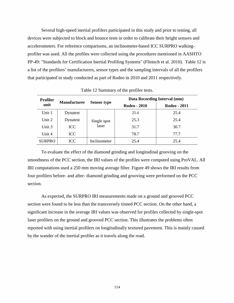
Several high-speed inertial profilers participated in this study and prior to testing, all
devices were subjected to block and bounce tests in order to calibrate their height sensors and
accelerometers. For reference comparisons, an inclinometer-based ICC SURPRO walking-
profiler was used. All the profiles were collected using the procedures mentioned in AASHTO
PP-49: "Standards for Certification Inertial Profiling Systems" (Flintsch et al. 2010). Table 12 is
a list of the profilers’ manufacturers, sensor types and the sampling intervals of all the profilers
that participated in study conducted as part of Rodeo in 2010 and 2011 respectively.
Table 12 Summary of the profiler tests.
Profiler unit Manufacturer Sensor type
Data Recording Interval (mm) Rodeo - 2010 Rodeo - 2011
Unit 1 Dynatest
Single spot laser
25.4 25.4
Unit 2 Dynatest 25.3 25.4
Unit 3 ICC 31.7 30.7
Unit 4 ICC 78.7 77.7
SURPRO ICC Inclinometer 25.4 25.4
To evaluate the effect of the diamond grinding and longitudinal grooving on the
smoothness of the PCC section, the IRI values of the profiles were computed using ProVAL. All
IRI computations used a 250 mm moving average filter. Figure 49 shows the IRI results from
four profilers before- and after- diamond grinding and grooving were performed on the PCC
section.
As expected, the SURPRO IRI measurements made on a ground and grooved PCC
section were found to be less than the transversely tinned PCC section. On the other hand, a
significant increase in the average IRI values was observed for profiles collected by single-spot
laser profilers on the ground and grooved PCC section. This illustrates the problems often
reported with using inertial profilers on longitudinally textured pavement. This is mainly caused
by the wander of the inertial profiler as it travels along the road.
114
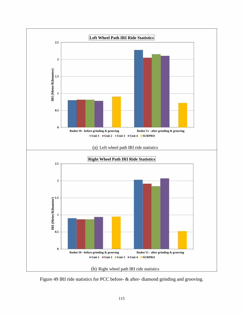
0
0.5
1
1.5
2
2.5
Rodeo'10 - before grinding & grooving Rodeo'11 - after grinding & grooving
IRI (
Met
er/K
ilom
eter
)
Left Wheel Path IRI Ride Statistics
Unit 1 Unit 2 Unit 3 Unit 4 SURPRO
(a) Left wheel path IRI ride statistics
0
0.5
1
1.5
2
2.5
Rodeo'10 - before grinding & grooving Rodeo'11 - after grinding & grooving
IRI (
Met
er/K
ilom
eter
)
Right Wheel Path IRI Ride Statistics
Unit 1 Unit 2 Unit 3 Unit 4 SURPRO
(b) Right wheel path IRI ride statistics
Figure 49 IRI ride statistics for PCC before- & after- diamond grinding and grooving.
115

Figure 50 shows the continuous roughness plots for profile collected by Unit 2 on the left
wheel path of ground and grooved PCC section against the corresponding SURPRO profile. The
plot shows that there are significant differences in the roughness distribution among the profiles
collected by the single spot laser profilers compared to the reference instrument. This difference
is caused by the presence of longitudinal grooves on the pavement surface, which causes the
height-sensor of the single spot laser profiler unit to obtain measurements at the bottom of the
groove as well as on the pavement surface because of lateral wander.
Error! Reference source not found. shows that there is very poor agreement between
the participant profile and the reference profile at short, medium and long wavebands
respectively. Since IRI is most sensitive in the wavelength range of 1 to 30 meter (4 to 100 feet)
(Karamihas et al. 1999), the participant profiles produced IRI that were significantly higher than
that measured by reference instrument.
The difference in PSD is attributed to the presence of the diamond ground texture and the
longitudinal grooves on PCC section which resulted in incorrect recording of the profile data by
the single-spot sensors of the participant units which introduced artificial wavelengths in the
profile and over-estimating the IRI values higher than the 'true' IRI of the pavement section
measured by the reference profiler (Figure 51, Figure 52, and Figure 53).
Figure 50 Continuous roughness distribution profile of Unit-2 and SURPRO on ground and grooved PCC section [Base-length = 7.6 meter (25 feet)].
116
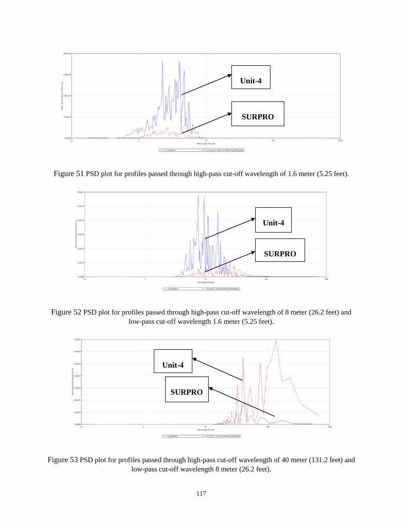
Figure 51 PSD plot for profiles passed through high-pass cut-off wavelength of 1.6 meter (5.25 feet).
Figure 52 PSD plot for profiles passed through high-pass cut-off wavelength of 8 meter (26.2 feet) and low-pass cut-off wavelength 1.6 meter (5.25 feet).
Figure 53 PSD plot for profiles passed through high-pass cut-off wavelength of 40 meter (131.2 feet) and low-pass cut-off wavelength 8 meter (26.2 feet).
SURPRO
Unit-4
Unit-4
SURPRO
Unit-4
SURPRO
117

FINDINGS AND CONCLUSIONS
The paper investigated the effect of diamond grinding and grooving on the surface characteristics
of PCC. Improvements in macrotexture, friction, and smoothness for a PCC pavement subjected
to diamond grinding and grooving was evaluated. Following is the summary of the findings and
conclusions of the study:
• Diamond grinding and grooving significantly increased the macrotexture of the PCC
surface. High macrotexture can aid in removing water from the pavement surface which
can cause hydroplaning and skidding problems during wet-weather condition.
• Friction measurements revealed that friction measured with the smooth tire increased
after applying diamond grinding and grooving to the PCC surface. This effect was found
to be more significant at higher speeds.
• Ribbed tire skid trailers results did not show a significant difference in friction
measurements made on the ground and grooved PCC compared to the tinned PCC. This
was expected as ribbed tire measurements are not very sensitive to pavement
macrotexture.
• SURPRO reference profiler results showed a decrease in IRI values on the PCC surface
after grooving. The improvement in smoothness was substantial on the right wheel path
with 19 mm (¾ inch) grooving compared to the left wheel path with 13 mm (½ inch)
grooves.
• Compared to the reference profiler, single spot laser profilers over-predicted the IRI
values on the ground and grooved PCC. This disagreement is thought to be due to
grooves on the section, which render the single-spot profilers incapable of measuring the
correct profile. PSD analysis confirmed the presence of artificial wavelengths in the
profiles collected by single spot laser profiler which is due to the longitudinal grooving.
The authors recommend using wide-footprint profiling systems in future research on pavement
with longitudinal grooves.
118

ACKNOWLEDGEMENTS
The data for this study was collected during the annual equipment rodeo as part of the Pavement
Surface Properties Consortium. The experiment has been made possible thanks to contribution
of the Virginia Tech Transportation Institute (VTTI), the Virginia Center for Transportation
Innovation and Research, the Federal Highway Administration (FHWA), the Connecticut,
Georgia, Mississippi, Pennsylvania, South Carolina, and Virginia DOTs. The authors would like
to thank William Hobbs, Stephen Valeri, Chris Tomlinson, and James Bryce for their
contribution in data collection and Grinding & Grooving L.D. for their support by grinding and
grooving the test sections at no charge to the study.
REFERENCES
Dare, T., W. Thornton, T. Wulf, and R. Bernhard. “Aucoustical Effects of Grinding and
Grooving on Portland Cement Concrete Pavements”, 2009. http://igga.net/technical-
information/technical-information.cfm?mode=display&article=9. Accessed July 20, 2011.
Flintsch, G. W., E. D. de León Izeppi, K. K. McGhee, and S. Najafi. “Speed Adjustment Factors
for Locked-Wheel Skid Trailer Measurements”. Transportation Research Record: Journal of the
Transportation Research Board, Volume 2155, Transportation Research Board of the National
Academies, Washington, D.C., 2010, pp. 117-123.
Flintsch, G. W., E. D. de León Izeppi, K. K. McGhee, and S. Shetty. “Profiler Certification
Process at the Virginia Smart Road”. Presented at the 89th Annual Meeting of the Transportation
Research Board, Washington D.C., 2010.
Karamihas, S. M., and J. K. Cable. “Developing Smooth, Quiet, Safe Portland Cement Concrete
Pavements”. Publication FHWA-DTFH61-01-X-002. FHWA, U.S. Department of
Transportation, 2004.
Karamihas, S. M., T. D. Gillespie, R. W. Perera, and S. D. Kohn. “Guidelines for longitudinal
pavement profile measurement”. NCHRP report 434, 1999.
119
Martinez, J. E.” Effects of pavement grooving on friction, braking, and vehicle control”.
Transportation Research Record: Journal of the Transportation Research Board, No. 633,
Transportation Research Board of the National Academies, Washington, D.C., 1977, pp. 8-13.
Perera, R. W., and S. D. Kohn. “Issues in pavement smoothness: A summary report”. NCHRP
Project 20-51(1), 2002.
Perera, R. W., S. D. Kohn, and L. J. Wiser. “Factors contributing to differences between profiler
and the international roughness index”. Transportation Research Record: Journal of the
Transportation Research Board, Volume 1974, Transportation Research Board of the National
Academies, Washington, D.C., 2006, pp. 81-88.
Perera, R.W., S.D. Kohn, and S. Bemanian. “Comparison of road profilers”. Transportation
Research Record: Journal of the Transportation Research Board, Volume 1536, Transportation
Research Board of the National Academies, Washington, D.C., 1996, pp. 117-124.
Roberts, J. H. “Virginia Smart Road: Newly constructed test sections will help researchers learn
more about grinding and grooving”. http://www.concreteconstruction.net/roads-and-
highways/virginia-smart-road.aspx, Accessed July 26, 2011.
Sayers, M. W., and S. M. Karamihas. “The Little Book of Profiling: Basic Information about
Measuring and Interpreting Road Profiles”. The Regent of the University of Michigan, 1998.
Scofield, L. “Safe, Smooth, and Quiet Concrete Pavement”. First International Conference on
Pavement Preservation, 2012. http://techtransfer.berkeley.edu/icpp. Accessed July 20, 2011.
Shahin, M.Y. “Pavement management for airports, roads, and parking lots”. Springer LLC., New
York, USA, 2005.
Wambold, J.C., J.J. Henry, and R.R. Hegmon. “Skid resistance of wet-weather accident sites”.
ASTM International, Philadelphia, USA, 1986.
Wulf, T., T. Dare, and R. Bernhard, “The effect of grinding and grooving on the noise generation
of Portland Cement Concrete pavement”. Journal of the Acoustical Society of America, 2008.
120
CHAPTER 7 - SUMMARY, FINDINGS, CONCLUSIONS, AND
RECOMMENDATIONS
It is important for highway agencies to monitor the pavement friction periodically and
systematically to support their safety management programs. The collected data can help
implement preservation policies that improve the safety of the roadway network and decrease the
number of skidding-related crashes. This dissertation evaluates different approaches to model the
relationship between vehicle crashes and friction and provides some guidelines on how to use
this relationship for managing pavement friction.
The study started with an extensive literature review on tire pavement friction and its
relationship to vehicle crashes. It then evaluated the effect of friction on wet and dry crashes
using both, traditional regression analysis and soft-computing approaches. The effectiveness of
diamond grinding and grooving technique for correcting friction deficiencies is also evaluated.
The main finding and conclusions of the study are summarized in this section.
FINDINGS
The results of chapter two show that friction is a significant factor affecting the ratios of both
wet- and dry-condition vehicle crashes. Contrary to other studies that only emphasize the effect
of friction on wet-condition crashes; this study revealed that friction impacts the rate of dry-
condition crashes as well. The normal probability plot of residuals and residual plots for
predicted values and regressors suggested, as expected, that the relation between friction and
vehicle crashes is not linear and that a logarithmic transformation was necessary for the data.
Transformation improved the coefficient of determination (R-square) of the models.
Two alternative soft-computing approaches to traditional regression were used in chapter
three and four: Artificial Neural Network and Fuzzy Logic. Both methods are capable of
predicting the crash rate based on friction, traffic volume and speed limit. Neural network
approach produces the highest precision (lowest MSE) compared to fuzzy logic and regression
method. The down side of neural networks is that it acts as a “black-box”. Fuzzy logic on the
121

other had is easy to understand as it used linguistic rules. Fuzzy logic rules also take less
computation spaces compared to neural network and regression and they can be easily stored on
microchips and vehicles’ ECU. This makes fuzzy logic approach more appropriate for real-time
application.
The learning ability of neural network is very sensitive to the learning rate which is
defined in the back-propagation algorithm. If the learning rate is set to high, the algorithm may
miss the global minimum. On the other hand, if the learning rate is set too high, the algorithm
may not converge. To handle the effect of learning rate in the traditional back-propagation
algorithm, three alternative learning algorithms were implanted: Levenberg-Marquardt,
conjugate gradient, and resilient back-propagation. Levenberg-Marquardt algorithm had highest
prediction accuracy (lowest MSE) and the fastest convergence time compared to conjugate
gradient and resilient back-propagation learning algorithm and was used to train the neural
network model in this study.
The results of ANN analysis show that the rate of wet crashes for sites with friction
number below 32 is 40 percent higher than sites with friction higher than networks average (45)
while for dry crashes the difference was approximately 15 percent. The effect of friction on
reducing the rate of wet crashes is more pronounced than dry crashes.
Fuzzy Logic Interface System provides another reliable tool for PFM decision making
process. The system can be easily modified based on agency needs. The model uses linguistic
and human like rules and it is easy to understand for practitioners and highway engineers. Crash
risk can be predicted based on friction, traffic and speed limit using both Mamdani and Sugeno
controllers. Mamdani controller produced a higher precision (lower MSE) than Sugeno. The
advantage of Sugeno system is that it can be used with other adaptive learning methods such as
backpropagation. Mamdani is using linguistic rules which is easier to use for decision making
purposes.
Fuzzy logic model also confirms that the rate of both wet and dry condition crashes
increase as the friction increases. Highest wet/dry crash rate was observed for friction number
below 30 and speed limit above 42 mph. Authors suggest using both wet and dry condition
crashes in PFM studies. Similar to neural network approach, investigatory threshold level of
122

friction can be defined based on the crash risk. Agency can modify the level based on the
available funding. This allows highway agencies to prioritize resources based on safety needs so
they can advance the resurfacing project if the site is already in the queue for resurfacing and the
crash risk is high. Application of the fuzzy system in real-time slipper spot warning system was
demonstrated as a proof of concept. Fuzzy systems take a very small storage space and they can
be easily stores on microchips or vehicles’ ECU.
Diamond grinding and grooving technique discussed in chapter six, significantly
increased the macrotexture of the PCC surface. High macrotexture can aid in removing water
from the pavement surface which can cause hydroplaning and skidding problems during wet-
weather condition. Friction measurements revealed that friction increased after applying
diamond grinding and grooving to the PCC surface, especially when using the smooth tire. This
effect was found to be more significant at higher speeds. Ribbed tire skid trailers results did not
show a significant difference in friction measurements made on the ground and grooved PCC
compared to the tinned PCC. This was expected as ribbed tire measurements are not very
sensitive to pavement macrotexture.
CONCLUSIONS
Friction is a significant factor affecting the rate of both wet and dry vehicle crashes. Dry crashes
should be considered along with wet crashes in future friction and safety studies. The
relationship between friction and crash rates can be used by DOTs and highway agencies to
define acceptable levels of friction for various types of roadways in their networks. It also
provides them a systemic way to prioritize projects for HSIP funds based on the crash rate.
Both ANN and Fuzzy Logic are valid approaches for developing a PFM. The benefit of
Fuzzy Logic over ANN and regression techniques is that it can be used for real-time application.
This allows the model to be used in connected vehicle applications. Real-time slippery spot
warning system can be developed using the sensors that are already installed in the vehicle. Such
a system can warn the drivers of potential hazardous condition so they can adjusts their speed
based on the available friction; especially in inclement weather condition. The system can also
be used in snow and ice removal operation to detect the areas that need plowing or chemical
treatment as well as monitoring the contractors plowing operation. Such data can be provided to
123
the citizens in form of a state-wide map. The routes can be color coded based on the real-time
available level of friction. This will allow citizens to select safe routes to commute.
RECOMMENDATIONS FOR FUTURE RESEARCH
Friction data is the heart of PFM. Collecting data with locked-wheel skid trailers can be a very
time consuming task. Further research needs to be done on implementing non-contact friction
measurement into PFM. Based on the literature review that was done in chapter 1, it seems that
vehicle dynamic-based friction estimation can be a good alternative to locked-wheel skid trailers.
It can be incorporated into regular fleet vehicles with minimal cost to the agency. The data
collection rate is also very high as it does not require water for testing.
More research needs to be done on the real-time slippery spot detection system. The
potential of the system in ice and snow removal operation need to be further investigate. Such a
system would allow the chemical and brine rate application to be adjusted based on the level of
available friction.
Factors such as seasonal variation and temperature changes can affect the friction
measurement. This effect needs to be further investigated and incorporated into the PFM
program. This will allow the agency to collect friction data throughout the year and make
correction based on the temperature/season to make comparison possible.
124
APPENDIX A – SAS CODE FOR CRASH ANALYSIS
data Project;
input Dry FN Speed Traffic;
lines;
.
.
.
;
run;
proc reg data=Project;
model Dry = FN Speed Traffic /clb clm cli ;
plot RESIDUAL.*PREDICTED.;
run;
proc reg data=Project;
model Dry = FN Speed Traffic /clb clm cli ;
plot Dry*FN Dry*Speed Dry*Traffic RESIDUAL.*FN RESIDUAL.*Speed RESIDUAL.*Traffic RESIDUAL.*PREDICTED.;
run;
125

APPENDIX B – MATLAB NEURAL NETWORK CODE FOR LEVENBERG-MARQUARDT LEARNING ALGORITHM
% Solve an Input-Output Fitting problem with a Neural Network
% Script generated by NFTOOL
% Created Sun Jun 14 09:39:52 EDT 2015
%
% This script assumes these variables are defined:
%
% NDRYINPUT - input data.
% NDRYOUTPUT - target data.
inputs = NDRYINPUT';
targets = NDRYOUTPUT';
% Create a Fitting Network
hiddenLayerSize = 8;
net = fitnet(hiddenLayerSize);
% Choose Input and Output Pre/Post-Processing Functions
% For a list of all processing functions type: help nnprocess
net.inputs{1}.processFcns = {'removeconstantrows','mapminmax'};
net.outputs{2}.processFcns = {'removeconstantrows','mapminmax'};
% Setup Division of Data for Training, Validation, Testing
% For a list of all data division functions type: help nndivide
net.divideFcn = 'dividerand'; % Divide data randomly
126

net.divideMode = 'sample'; % Divide up every sample
net.divideParam.trainRatio = 70/100;
net.divideParam.valRatio = 15/100;
net.divideParam.testRatio = 15/100;
% For help on training function 'trainlm' type: help trainlm
% For a list of all training functions type: help nntrain
net.trainFcn = 'trainlm'; % Levenberg-Marquardt
% Choose a Performance Function
% For a list of all performance functions type: help nnperformance
net.performFcn = 'mse'; % Mean squared error
% Choose Plot Functions
% For a list of all plot functions type: help nnplot
net.plotFcns = {'plotperform','plottrainstate','ploterrhist', ...
'plotregression', 'plotfit'};
% Train the Network
[net,tr] = train(net,inputs,targets);
% Test the Network
outputs = net(inputs);
errors = gsubtract(targets,outputs);
performance = perform(net,targets,outputs)
127

% Recalculate Training, Validation and Test Performance
trainTargets = targets .* tr.trainMask{1};
valTargets = targets .* tr.valMask{1};
testTargets = targets .* tr.testMask{1};
trainPerformance = perform(net,trainTargets,outputs)
valPerformance = perform(net,valTargets,outputs)
testPerformance = perform(net,testTargets,outputs)
% View the Network
view(net)
% Plots
% Uncomment these lines to enable various plots.
%figure, plotperform(tr)
%figure, plottrainstate(tr)
%figure, plotfit(net,inputs,targets)
%figure, plotregression(targets,outputs)
%figure, ploterrhist(errors)
128

APPENDIX C – MATLAB NEURAL NETWORK CODE FOR CONJUGATE GRADIENT LEARNING ALGORITHM
% Solve an Input-Output Fitting problem with a Neural Network
% Script generated by NFTOOL
% Created Sun Jun 14 09:39:52 EDT 2015
%
% This script assumes these variables are defined:
%
% NDRYINPUT - input data.
% NDRYOUTPUT - target data.
inputs = NDRYINPUT';
targets = NDRYOUTPUT';
% Create a Fitting Network
hiddenLayerSize = 8;
net = fitnet(hiddenLayerSize);
% Choose Input and Output Pre/Post-Processing Functions
% For a list of all processing functions type: help nnprocess
net.inputs{1}.processFcns = {'removeconstantrows','mapminmax'};
net.outputs{2}.processFcns = {'removeconstantrows','mapminmax'};
% Setup Division of Data for Training, Validation, Testing
% For a list of all data division functions type: help nndivide
net.divideFcn = 'dividerand'; % Divide data randomly
129

net.divideMode = 'sample'; % Divide up every sample
net.divideParam.trainRatio = 70/100;
net.divideParam.valRatio = 15/100;
net.divideParam.testRatio = 15/100;
% For help on training function 'trainscg' type: help trainscg
% For a list of all training functions type: help nntrain
net.trainFcn = 'trainscg'; % Conjugate-Gradient
% Choose a Performance Function
% For a list of all performance functions type: help nnperformance
net.performFcn = 'mse'; % Mean squared error
% Choose Plot Functions
% For a list of all plot functions type: help nnplot
net.plotFcns = {'plotperform','plottrainstate','ploterrhist', ...
'plotregression', 'plotfit'};
% Train the Network
[net,tr] = train(net,inputs,targets);
% Test the Network
outputs = net(inputs);
errors = gsubtract(targets,outputs);
performance = perform(net,targets,outputs)
130

% Recalculate Training, Validation and Test Performance
trainTargets = targets .* tr.trainMask{1};
valTargets = targets .* tr.valMask{1};
testTargets = targets .* tr.testMask{1};
trainPerformance = perform(net,trainTargets,outputs)
valPerformance = perform(net,valTargets,outputs)
testPerformance = perform(net,testTargets,outputs)
% View the Network
view(net)
% Plots
% Uncomment these lines to enable various plots.
%figure, plotperform(tr)
%figure, plottrainstate(tr)
%figure, plotfit(net,inputs,targets)
%figure, plotregression(targets,outputs)
%figure, ploterrhist(errors)
131

APPENDIX D – MATLAB NEURAL NETWORK CODE FOR RESILIENT BACK PROPAGATION LEARNING ALGORITHM
% Solve an Input-Output Fitting problem with a Neural Network
% Script generated by NFTOOL
% Created Sun Jun 14 09:39:52 EDT 2015
%
% This script assumes these variables are defined:
%
% NDRYINPUT - input data.
% NDRYOUTPUT - target data.
inputs = NDRYINPUT';
targets = NDRYOUTPUT';
% Create a Fitting Network
hiddenLayerSize = 8;
net = fitnet(hiddenLayerSize);
% Choose Input and Output Pre/Post-Processing Functions
% For a list of all processing functions type: help nnprocess
net.inputs{1}.processFcns = {'removeconstantrows','mapminmax'};
net.outputs{2}.processFcns = {'removeconstantrows','mapminmax'};
% Setup Division of Data for Training, Validation, Testing
% For a list of all data division functions type: help nndivide
net.divideFcn = 'dividerand'; % Divide data randomly
132

net.divideMode = 'sample'; % Divide up every sample
net.divideParam.trainRatio = 70/100;
net.divideParam.valRatio = 15/100;
net.divideParam.testRatio = 15/100;
% For help on training function 'trainrp' type: help trainrp
% For a list of all training functions type: help nntrain
net.trainFcn = 'trainrp'; % Resilient-Back-Propagation
% Choose a Performance Function
% For a list of all performance functions type: help nnperformance
net.performFcn = 'mse'; % Mean squared error
% Choose Plot Functions
% For a list of all plot functions type: help nnplot
net.plotFcns = {'plotperform','plottrainstate','ploterrhist', ...
'plotregression', 'plotfit'};
% Train the Network
[net,tr] = train(net,inputs,targets);
% Test the Network
outputs = net(inputs);
errors = gsubtract(targets,outputs);
performance = perform(net,targets,outputs)
133

% Recalculate Training, Validation and Test Performance
trainTargets = targets .* tr.trainMask{1};
valTargets = targets .* tr.valMask{1};
testTargets = targets .* tr.testMask{1};
trainPerformance = perform(net,trainTargets,outputs)
valPerformance = perform(net,valTargets,outputs)
testPerformance = perform(net,testTargets,outputs)
% View the Network
view(net)
% Plots
% Uncomment these lines to enable various plots.
%figure, plotperform(tr)
%figure, plottrainstate(tr)
%figure, plotfit(net,inputs,targets)
%figure, plotregression(targets,outputs)
%figure, ploterrhist(errors)
134

APPENDIX E – MATLAB NEURAL NETWORK CODE FOR DRY CRASH PREDICTION
% Solve an Input-Output Fitting problem with a Neural Network
% Script generated by NFTOOL
% Created Sun Jun 14 09:39:52 EDT 2015
%
% This script assumes these variables are defined:
%
% NDRYINPUT - input data.
% NDRYOUTPUT - target data.
inputs = NDRYINPUT';
targets = NDRYOUTPUT';
% Create a Fitting Network
hiddenLayerSize = 8;
net = fitnet(hiddenLayerSize);
% Choose Input and Output Pre/Post-Processing Functions
% For a list of all processing functions type: help nnprocess
net.inputs{1}.processFcns = {'removeconstantrows','mapminmax'};
net.outputs{2}.processFcns = {'removeconstantrows','mapminmax'};
% Setup Division of Data for Training, Validation, Testing
% For a list of all data division functions type: help nndivide
135

net.divideFcn = 'dividerand'; % Divide data randomly
net.divideMode = 'sample'; % Divide up every sample
net.divideParam.trainRatio = 70/100;
net.divideParam.valRatio = 15/100;
net.divideParam.testRatio = 15/100;
% For help on training function 'trainlm' type: help trainlm
% For a list of all training functions type: help nntrain
net.trainFcn = 'trainlm'; % Levenberg-Marquardt
% Choose a Performance Function
% For a list of all performance functions type: help nnperformance
net.performFcn = 'mse'; % Mean squared error
% Choose Plot Functions
% For a list of all plot functions type: help nnplot
net.plotFcns = {'plotperform','plottrainstate','ploterrhist', ...
'plotregression', 'plotfit'};
% Train the Network
[net,tr] = train(net,inputs,targets);
% Test the Network
outputs = net(inputs);
errors = gsubtract(targets,outputs);
performance = perform(net,targets,outputs)
136

% Recalculate Training, Validation and Test Performance
trainTargets = targets .* tr.trainMask{1};
valTargets = targets .* tr.valMask{1};
testTargets = targets .* tr.testMask{1};
trainPerformance = perform(net,trainTargets,outputs)
valPerformance = perform(net,valTargets,outputs)
testPerformance = perform(net,testTargets,outputs)
% View the Network
view(net)
% Plots
% Uncomment these lines to enable various plots.
%figure, plotperform(tr)
%figure, plottrainstate(tr)
%figure, plotfit(net,inputs,targets)
%figure, plotregression(targets,outputs)
%figure, ploterrhist(errors)
137

APPENDIX F – MATLAB NEURAL NETWORK CODE FOR WET CRASH PREDICTION
% Solve an Input-Output Fitting problem with a Neural Network
% Script generated by NFTOOL
% Created Sun Jun 14 10:30:52 EDT 2015
%
% This script assumes these variables are defined:
%
% NWETINPUT - input data.
% NWETOUTPUT - target data.
inputs = NWETINPUT';
targets = NWETOUTPUT';
% Create a Fitting Network
hiddenLayerSize = 8;
net = fitnet(hiddenLayerSize);
% Choose Input and Output Pre/Post-Processing Functions
% For a list of all processing functions type: help nnprocess
net.inputs{1}.processFcns = {'removeconstantrows','mapminmax'};
net.outputs{2}.processFcns = {'removeconstantrows','mapminmax'};
% Setup Division of Data for Training, Validation, Testing
% For a list of all data division functions type: help nndivide
net.divideFcn = 'dividerand'; % Divide data randomly
138

net.divideMode = 'sample'; % Divide up every sample
net.divideParam.trainRatio = 70/100;
net.divideParam.valRatio = 15/100;
net.divideParam.testRatio = 15/100;
% For help on training function 'trainlm' type: help trainlm
% For a list of all training functions type: help nntrain
net.trainFcn = 'trainlm'; % Levenberg-Marquardt
% Choose a Performance Function
% For a list of all performance functions type: help nnperformance
net.performFcn = 'mse'; % Mean squared error
% Choose Plot Functions
% For a list of all plot functions type: help nnplot
net.plotFcns = {'plotperform','plottrainstate','ploterrhist', ...
'plotregression', 'plotfit'};
% Train the Network
[net,tr] = train(net,inputs,targets);
% Test the Network
outputs = net(inputs);
errors = gsubtract(targets,outputs);
performance = perform(net,targets,outputs)
139

% Recalculate Training, Validation and Test Performance
trainTargets = targets .* tr.trainMask{1};
valTargets = targets .* tr.valMask{1};
testTargets = targets .* tr.testMask{1};
trainPerformance = perform(net,trainTargets,outputs)
valPerformance = perform(net,valTargets,outputs)
testPerformance = perform(net,testTargets,outputs)
% View the Network
view(net)
% Plots
% Uncomment these lines to enable various plots.
%figure, plotperform(tr)
%figure, plottrainstate(tr)
%figure, plotfit(net,inputs,targets)
%figure, plotregression(targets,outputs)
%figure, ploterrhist(errors)
140

APPENDIX G – MATLAB CODE FOR MAMDANI FUZZY INFERENCE SYSTEM
[System]
Name='Crash_Predictor_September'
Type='mamdani'
Version=2.0
NumInputs=3
NumOutputs=2
NumRules=7
AndMethod='min'
OrMethod='max'
ImpMethod='min'
AggMethod='max'
DefuzzMethod='centroid'
[Input1]
Name='Friction'
Range=[0 100]
NumMFs=5
MF1='Very-Low':'trimf',[10 20 30]
MF2='Low':'trimf',[20 30 40]
MF3='Medium':'trimf',[30 40 50]
MF4='High':'trimf',[40 50 60]
MF5='Very-High':'trimf',[50 60 70]
[Input2]
Name='AADT'
141

Range=[0 20]
NumMFs=3
MF1='Low':'trimf',[10 12 14]
MF2='Medium':'trimf',[12 14 16]
MF3='High':'trimf',[14 16 18.3]
[Input3]
Name='Speed-Limit'
Range=[0 70]
NumMFs=3
MF1='Low':'trimf',[33.5 38 42.5]
MF2='Medium':'trimf',[38 42.5 47]
MF3='High':'trimf',[42.5 47 51.5]
[Output1]
Name='Dry-Condition-Crashes'
Range=[0 1]
NumMFs=5
MF1='Very-Low-Risk':'trimf',[0 0.075 0.15]
MF2='Low-Risk':'trimf',[0.05 0.2 0.35]
MF3='Medium-Risk':'trimf',[0.25 0.4 0.55]
MF4='High-Risk':'trimf',[0.45 0.6 0.75]
MF5='Very-High-Risk':'trimf',[0.65 0.8 1]
[Output2]
Name='Wet-Condition-Crashes'
Range=[0 1]
NumMFs=5
142

MF1='Very-Low':'trimf',[0 0.075 0.15]
MF2='Low':'trimf',[0.05 0.2 0.35]
MF3='Medium':'trimf',[0.25 0.4 0.55]
MF4='High':'trimf',[0.45 0.6 0.75]
MF5='Very-High':'trimf',[0.65 0.8 1]
[Rules]
1 2 2, 5 5 (1) : 1
2 2 3, 5 5 (1) : 1
2 2 1, 5 4 (1) : 1
3 3 3, 3 3 (1) : 1
4 3 3, 2 1 (1) : 1
5 1 3, 2 3 (1) : 1
5 2 3, 2 1 (1) : 1
143

APPENDIX H – SUGENO FUZZY INFERENCE SYSTEM FOR DRY CRASH PREDICTION
[System]
Name='Nafise_Dry'
Type='sugeno'
Version=2.0
NumInputs=3
NumOutputs=1
NumRules=45
AndMethod='prod'
OrMethod='probor'
ImpMethod='prod'
AggMethod='sum'
DefuzzMethod='wtaver'
[Input1]
Name='Friction'
Range=[20 64]
NumMFs=5
MF1='in1mf1':'trapmf',[12.3 16.7 23.299988423472 27.69998201196]
MF2='in1mf2':'trapmf',[23.2999913854456 27.6999884234771 34.3000001393631 38.7000017765564]
MF3='in1mf3':'trapmf',[34.299999713892 38.7000001393631 45.3000031421955 49.7000042369533]
MF4='in1mf4':'trapmf',[45.3000044863956 49.7000031421965 56.2999960844553 60.6999971286629]
MF5='in1mf5':'trapmf',[56.2999939031986 60.6999960844557 67.3 71.7]
144

[Input2]
Name='Speed-Limit'
Range=[11.42079221 18.22254035]
NumMFs=3
MF1='in2mf1':'trapmf',[9.040180361 10.400529989 12.440997521194 13.8012891780393]
MF2='in2mf2':'trapmf',[12.4410049098752 13.8013471501842 15.8419567211799 17.2023701298859]
MF3='in2mf3':'trapmf',[15.8419574700658 17.2023063498596 19.242802571 20.603152199]
[Input3]
Name='input3'
Range=[39.73809524 48.73275862]
NumMFs=3
MF1='in3mf1':'trapmf',[36.589963057 38.388895733 41.0872977751319 42.8862403427283]
MF2='in3mf2':'trapmf',[41.0872938627281 42.8862304510758 45.5846268839716 47.3835609463655]
MF3='in3mf3':'trapmf',[45.584623650545 47.3835595599716 50.081958127 51.880890803]
[Output1]
Name='output'
Range=[0 1]
NumMFs=45
MF1='out1mf1':'linear',[0.00482983408312524 0.00241910201291762 0.00738186179956265 0.000185762849350971]
MF2='out1mf2':'linear',[0 0 0 0]
MF3='out1mf3':'linear',[0 0 0 0]
MF4='out1mf4':'linear',[0.00429153397174817 0.00231932434127984 0.00692165551907249 0.000171821505095094]
145

MF5='out1mf5':'linear',[0.00774921472988964 0.00547356549175409 0.0156310511296665 0.000364552331974243]
MF6='out1mf6':'linear',[0 0 0 0]
MF7='out1mf7':'linear',[0 0 0 0]
MF8='out1mf8':'linear',[0 0 0 0]
MF9='out1mf9':'linear',[0 0 0 0]
MF10='out1mf10':'linear',[0.0082376476839911 0.00411550487042829 0.0125847002956306 0.000315275713612044]
MF11='out1mf11':'linear',[0.00219454867212264 0.00105868258945856 0.00333234431484177 7.83767382900944e-005]
MF12='out1mf12':'linear',[0 0 0 0]
MF13='out1mf13':'linear',[0.0145211014250384 0.00697872443637483 0.0213204217838228 0.000518523099829214]
MF14='out1mf14':'linear',[0.00556025858556883 0.00276111206396054 0.00945121565793634 0.000234670268558178]
MF15='out1mf15':'linear',[0 0 0 0]
MF16='out1mf16':'linear',[0 0 0 0]
MF17='out1mf17':'linear',[0.00100412355738779 0.000443472611202026 0.00121200632622665 2.66692733163315e-005]
MF18='out1mf18':'linear',[0 0 0 0]
MF19='out1mf19':'linear',[0 0 0 0]
MF20='out1mf20':'linear',[0 0 0 0]
MF21='out1mf21':'linear',[0 0 0 0]
MF22='out1mf22':'linear',[0 0 0 0]
MF23='out1mf23':'linear',[0.00338953082843443 0.00144404394840397 0.00395874264436442 8.66534953146861e-005]
MF24='out1mf24':'linear',[0.00222481054798854 0.000794432831736099 0.00224246153631363 4.76514409483934e-005]
MF25='out1mf25':'linear',[0 0 0 0]
MF26='out1mf26':'linear',[0.00251293316833102 0.00107006454056108 0.00311835875032929 6.87018128780091e-005]
MF27='out1mf27':'linear',[0.00277898002135836 0.000933419637214528 0.00271934694409705 5.72906193084864e-005]
146

MF28='out1mf28':'linear',[0 0 0 0]
MF29='out1mf29':'linear',[0 0 0 0]
MF30='out1mf30':'linear',[0 0 0 0]
MF31='out1mf31':'linear',[0 0 0 0]
MF32='out1mf32':'linear',[0.000121176044053968 4.3905333757998e-005 0.000123359374416825 2.63426182726018e-006]
MF33='out1mf33':'linear',[0.000921517937405561 0.000370152921882098 0.0010206527185091 2.18984276634642e-005]
MF34='out1mf34':'linear',[0 0 0 0]
MF35='out1mf35':'linear',[0.000186797058895674 6.76815890455568e-005 0.000190162738090462 4.06080562816683e-006]
MF36='out1mf36':'linear',[-0.00274233714339715 -0.000705296340087817 -0.00185940623250555 -3.55253492177377e-005]
MF37='out1mf37':'linear',[0 0 0 0]
MF38='out1mf38':'linear',[0.00304837112329041 0.00054398145590725 0.00210008521983716 4.76307988014126e-005]
MF39='out1mf39':'linear',[0 0 0 0]
MF40='out1mf40':'linear',[0 0 0 0]
MF41='out1mf41':'linear',[0.00108181007556809 0.000251042480461975 0.000790849845694004 1.74485496059369e-005]
MF42='out1mf42':'linear',[-0.000514634485619607 -0.000145195713512136 -0.000427242336129284 -8.79050386544379e-006]
MF43='out1mf43':'linear',[0 0 0 0]
MF44='out1mf44':'linear',[0 0 0 0]
MF45='out1mf45':'linear',[-0.000719090641267726 -0.000207233383704046 -0.000603144353934947 -1.23919724751366e-005]
[Rules]
1 1 1, 1 (1) : 1
1 1 2, 2 (1) : 1
1 1 3, 3 (1) : 1
1 2 1, 4 (1) : 1
147

1 2 2, 5 (1) : 1
1 2 3, 6 (1) : 1
1 3 1, 7 (1) : 1
1 3 2, 8 (1) : 1
1 3 3, 9 (1) : 1
2 1 1, 10 (1) : 1
2 1 2, 11 (1) : 1
2 1 3, 12 (1) : 1
2 2 1, 13 (1) : 1
2 2 2, 14 (1) : 1
2 2 3, 15 (1) : 1
2 3 1, 16 (1) : 1
2 3 2, 17 (1) : 1
2 3 3, 18 (1) : 1
3 1 1, 19 (1) : 1
3 1 2, 20 (1) : 1
3 1 3, 21 (1) : 1
3 2 1, 22 (1) : 1
3 2 2, 23 (1) : 1
3 2 3, 24 (1) : 1
3 3 1, 25 (1) : 1
3 3 2, 26 (1) : 1
3 3 3, 27 (1) : 1
4 1 1, 28 (1) : 1
4 1 2, 29 (1) : 1
4 1 3, 30 (1) : 1
4 2 1, 31 (1) : 1
4 2 2, 32 (1) : 1
148
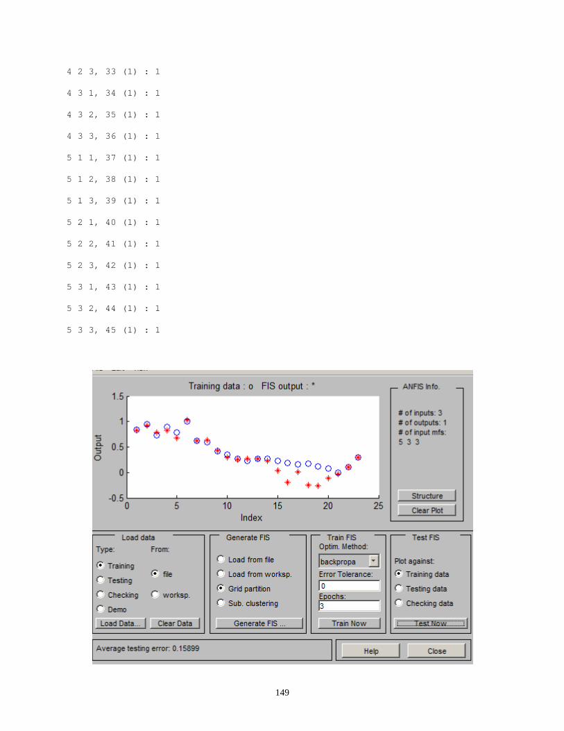
4 2 3, 33 (1) : 1
4 3 1, 34 (1) : 1
4 3 2, 35 (1) : 1
4 3 3, 36 (1) : 1
5 1 1, 37 (1) : 1
5 1 2, 38 (1) : 1
5 1 3, 39 (1) : 1
5 2 1, 40 (1) : 1
5 2 2, 41 (1) : 1
5 2 3, 42 (1) : 1
5 3 1, 43 (1) : 1
5 3 2, 44 (1) : 1
5 3 3, 45 (1) : 1
149
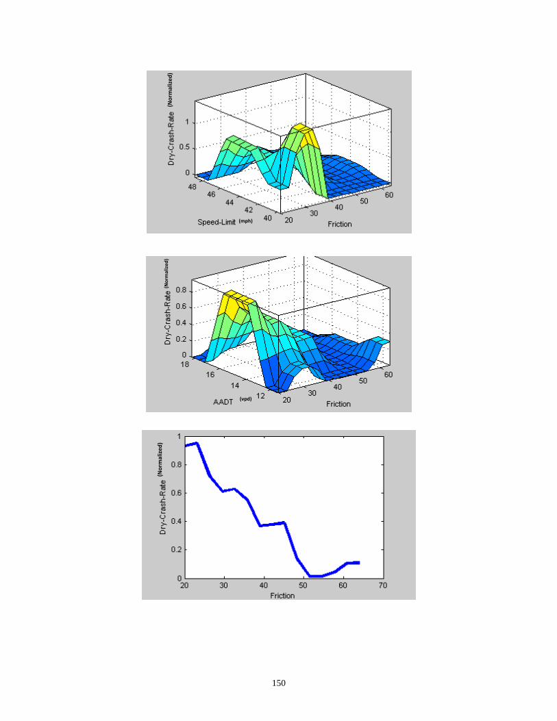
(mph)
(Nor
mal
ized
)
(vpd)
(Nor
mal
ized
)
(Nor
mal
ized
)
150

APPENDIX I – SUGENO FUZZY INFERENCE SYSTEM FOR WET CRASH PREDICTION
[System]
Name='Nafise_Wet'
Type='sugeno'
Version=2.0
NumInputs=3
NumOutputs=1
NumRules=45
AndMethod='prod'
OrMethod='probor'
ImpMethod='prod'
AggMethod='sum'
DefuzzMethod='wtaver'
[Input1]
Name='Friction'
Range=[20 64]
NumMFs=5
MF1='in1mf1':'trapmf',[12.3 16.7 23.2999926542859 27.6999887502761]
MF2='in1mf2':'trapmf',[23.299993987022 27.6999926542881 34.2999996917995 38.7000014539204]
MF3='in1mf3':'trapmf',[34.2999990153264 38.6999996917994 45.3000050679573 49.7000074719509]
MF4='in1mf4':'trapmf',[45.3000051116814 49.7000050679593 56.2999941172106 60.6999962171955]
MF5='in1mf5':'trapmf',[56.299990680464 60.6999941172114 67.3 71.7]
151

[Input2]
Name='Speed-Limit'
Range=[11.42079221 18.22254035]
NumMFs=3
MF1='in2mf1':'trapmf',[9.040180361 10.400529989 12.4409981989535 13.8012669812085]
MF2='in2mf2':'trapmf',[12.4410141884075 13.8013478279169 15.8419750775997 17.2024298851188]
MF3='in2mf3':'trapmf',[15.8419735885896 17.2023247073738 19.242802571 20.603152199]
[Input3]
Name='input3'
Range=[39.73809524 48.67605634]
NumMFs=3
MF1='in3mf1':'trapmf',[36.589963057 38.388895733 41.0873110699916 42.8862693961987]
MF2='in3mf2':'trapmf',[41.0873000914189 42.8862437460096 45.584626483101 47.3835603507286]
MF3='in3mf3':'trapmf',[45.5846230049706 47.3835591591014 50.081958127 51.880890803]
[Output1]
Name='Wet-Crash-Rate'
Range=[0.001799903 1]
NumMFs=45
MF1='out1mf1':'linear',[0.00403585142156673 0.00202142270929338 0.00616834800633493 0.000155225054675644]
MF2='out1mf2':'linear',[0 0 0 0]
MF3='out1mf3':'linear',[0 0 0 0]
MF4='out1mf4':'linear',[0.00345798277984982 0.00194386775518549 0.00576956653201852 0.000143083452024022]
152

MF5='out1mf5':'linear',[0.00724810793531277 0.00551435616068157 0.0154717100940833 0.000361109545183596]
MF6='out1mf6':'linear',[0 0 0 0]
MF7='out1mf7':'linear',[0 0 0 0]
MF8='out1mf8':'linear',[0 0 0 0]
MF9='out1mf9':'linear',[0 0 0 0]
MF10='out1mf10':'linear',[0.00719069271349823 0.00358716987421002 0.0109824220126841 0.000274420054754571]
MF11='out1mf11':'linear',[0.00302350440531358 0.0014585830397467 0.00459108419144812 0.000107982300189771]
MF12='out1mf12':'linear',[0 0 0 0]
MF13='out1mf13':'linear',[0.014526102711803 0.00693713135542547 0.021248087766914 0.000514558433407573]
MF14='out1mf14':'linear',[0.0047955312617654 0.00242737540490173 0.00889256196078528 0.000225664587078229]
MF15='out1mf15':'linear',[0 0 0 0]
MF16='out1mf16':'linear',[0 0 0 0]
MF17='out1mf17':'linear',[0.000981038722402203 0.000429860312852655 0.0011658452677155 2.56026359544277e-005]
MF18='out1mf18':'linear',[0 0 0 0]
MF19='out1mf19':'linear',[0 0 0 0]
MF20='out1mf20':'linear',[0 0 0 0]
MF21='out1mf21':'linear',[0 0 0 0]
MF22='out1mf22':'linear',[0 0 0 0]
MF23='out1mf23':'linear',[0.00354957461140924 0.00152512508099454 0.0041584498053195 9.10943688226852e-005]
MF24='out1mf24':'linear',[0.00207266541538367 0.000734634786084428 0.00207859812273166 4.40582454067726e-005]
MF25='out1mf25':'linear',[0 0 0 0]
MF26='out1mf26':'linear',[0.00253364239779784 0.00112701312133315 0.00329875546644942 7.32022177485687e-005]
MF27='out1mf27':'linear',[0.00192058462353626 0.00058939268034942 0.00179746735894887 3.73230510099656e-005]
153

MF28='out1mf28':'linear',[0 0 0 0]
MF29='out1mf29':'linear',[0 0 0 0]
MF30='out1mf30':'linear',[0 0 0 0]
MF31='out1mf31':'linear',[0 0 0 0]
MF32='out1mf32':'linear',[8.17374198106952e-005 2.96156614562187e-005 8.32101514207051e-005 1.77690043066729e-006]
MF33='out1mf33':'linear',[-0.000473899476754339 -7.61244243379448e-005 -0.000323836694471694 -6.2133892448134e-006]
MF34='out1mf34':'linear',[0 0 0 0]
MF35='out1mf35':'linear',[0.000126012836731792 4.56578335899244e-005 0.000128283315642819 2.73940949416939e-006]
MF36='out1mf36':'linear',[-0.00314994497541608 -0.000839999484946351 -0.00221130774295487 -4.25222871314913e-005]
MF37='out1mf37':'linear',[0 0 0 0]
MF38='out1mf38':'linear',[0.00543718910761521 0.000970265734446074 0.00374579079139064 8.49560798064877e-005]
MF39='out1mf39':'linear',[0 0 0 0]
MF40='out1mf40':'linear',[0 0 0 0]
MF41='out1mf41':'linear',[1.82751362894918e-005 4.24088816374305e-006 1.33599132056446e-005 2.94760262733742e-007]
MF42='out1mf42':'linear',[0.00176443506867425 0.000467236458182481 0.00142151827202665 2.9372084557417e-005]
MF43='out1mf43':'linear',[0 0 0 0]
MF44='out1mf44':'linear',[0 0 0 0]
MF45='out1mf45':'linear',[1.89857980309647e-005 2.36328141221602e-006 1.15229308967072e-005 2.49261733181951e-007]
[Rules]
1 1 1, 1 (1) : 1
1 1 2, 2 (1) : 1
1 1 3, 3 (1) : 1
1 2 1, 4 (1) : 1
154

1 2 2, 5 (1) : 1
1 2 3, 6 (1) : 1
1 3 1, 7 (1) : 1
1 3 2, 8 (1) : 1
1 3 3, 9 (1) : 1
2 1 1, 10 (1) : 1
2 1 2, 11 (1) : 1
2 1 3, 12 (1) : 1
2 2 1, 13 (1) : 1
2 2 2, 14 (1) : 1
2 2 3, 15 (1) : 1
2 3 1, 16 (1) : 1
2 3 2, 17 (1) : 1
2 3 3, 18 (1) : 1
3 1 1, 19 (1) : 1
3 1 2, 20 (1) : 1
3 1 3, 21 (1) : 1
3 2 1, 22 (1) : 1
3 2 2, 23 (1) : 1
3 2 3, 24 (1) : 1
3 3 1, 25 (1) : 1
3 3 2, 26 (1) : 1
3 3 3, 27 (1) : 1
4 1 1, 28 (1) : 1
4 1 2, 29 (1) : 1
4 1 3, 30 (1) : 1
4 2 1, 31 (1) : 1
4 2 2, 32 (1) : 1
155

4 2 3, 33 (1) : 1
4 3 1, 34 (1) : 1
4 3 2, 35 (1) : 1
4 3 3, 36 (1) : 1
5 1 1, 37 (1) : 1
5 1 2, 38 (1) : 1
5 1 3, 39 (1) : 1
5 2 1, 40 (1) : 1
5 2 2, 41 (1) : 1
5 2 3, 42 (1) : 1
5 3 1, 43 (1) : 1
5 3 2, 44 (1) : 1
5 3 3, 45 (1) : 1
156
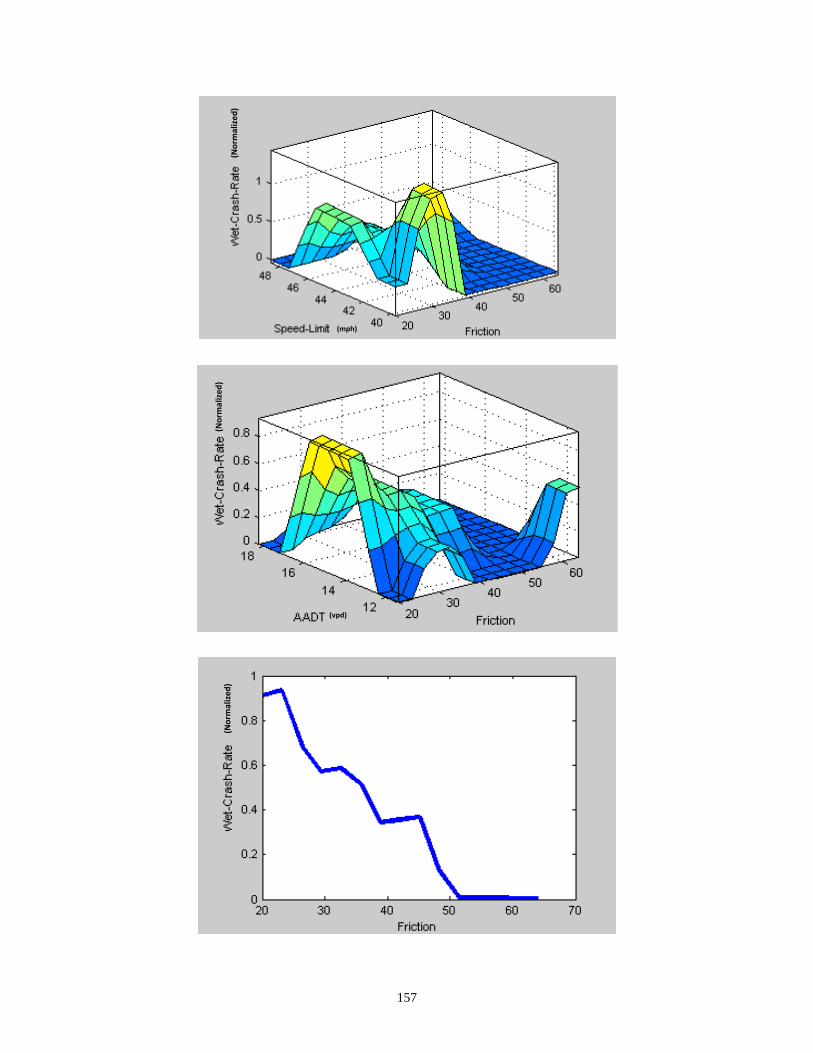
(mph)
(Nor
mal
ized
)
(vpd)
(Nor
mal
ized
)
(Nor
mal
ized
)
157

APPENDIX J – CARSIM SIMULATION INPUTS
158
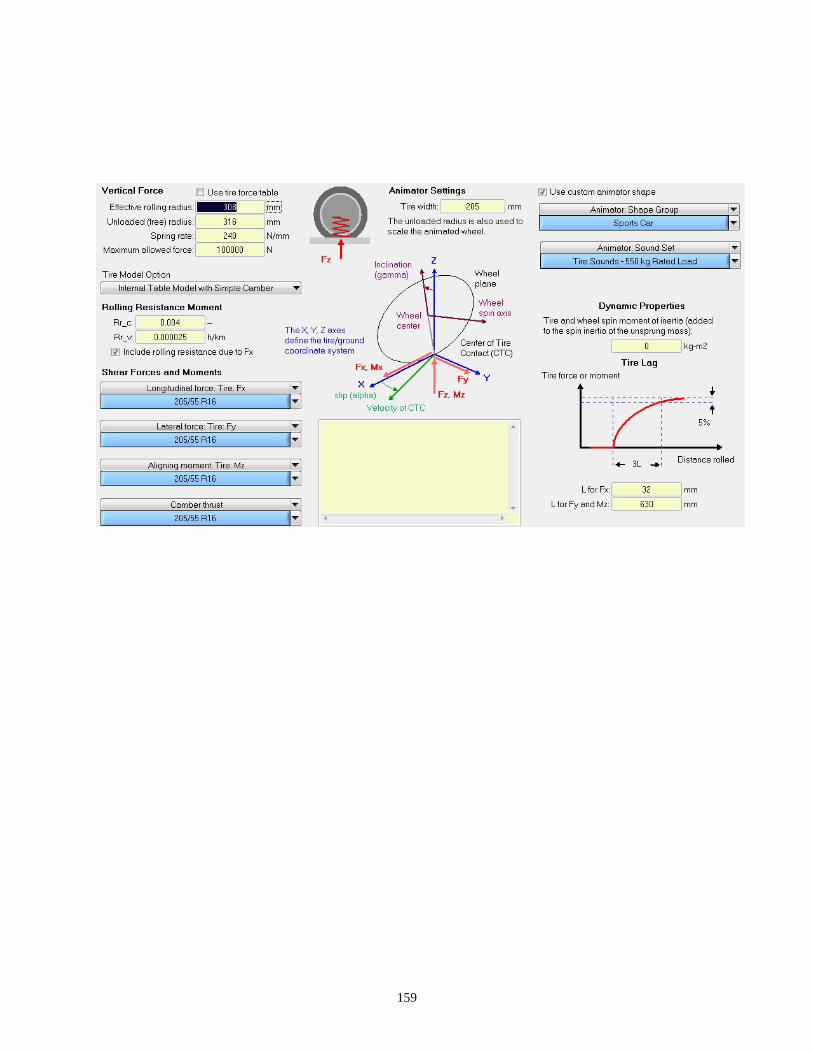
159