pavement performance monitoring using dynamic …

PAVEMENT PERFORMANCE MONITORING USING DYNAMIC CONE

PENETROMETER AND GEOGAUGE DURING CONSTRUCTION

by

AHMED NAWAL AHSAN

Presented to the Faculty of the Graduate School of

The University of Texas at Arlington in Partial Fulfillment

of the Requirements

for the Degree of

MASTER OF SCIENCE IN CIVIL ENGINEERING

THE UNIVERSITY OF TEXAS AT ARLINGTON

December 2014

iii

ACKNOWLEDGEMENTS

First, I would like to express my deepest gratitude to my supervisor Dr. Sahadat Hossain,

for his valuable time, guidance, encouragement, help and unconditional support throughout

my Master’s studies. Without his guidance and support throughout my Master’s study, this

thesis would not have been completed.

I would like to give my special thanks to Dr. Stefan A. Romanoschi and Dr. Xinbao Yu, for

their time and participation as my committee members and for their valuable suggestions

and advice.

My utmost appreciation to Texas Department of Transportation (TxDOT) for their constant

help and collaboration at site.

I am really grateful to Dr. Sadik Khan for his constant guidance, valuable input, cooperation

and assistance in all stages of work.

Special thanks extended to Dr. Golam Kibria, Dr. Sonia Samir, Mohammad Faysal, Asif

Ahmed, Masrur Mahedi and all my colleagues for their active cooperation and assistance.

Finally, and most of all, I would like to thank my parents for all their love, encouragement,

and great support.

November 12, 2014

iv

ABSTRACT

PAVEMENT PERFORMANCE MONITORING USING DYNAMIC CONE

PENETROMETER AND GEOGAUGE DURING CONSTRUCTION

Ahmed Nawal Ahsan

The University of Texas at Arlington, 2014

Supervising Professor: Sahadat Hossain

Proper design life of road network system requires adequate quality control

measures during the construction process to ensure proper material quality and sufficient

strength in between the materials. Laboratory tests are often time consuming and

sometimes, are not practical while the construction work is going on, in-situ techniques can

efficiently evaluate the material properties through simple and less time consuming

procedures. Dynamic Cone Penetrometer and Geogauge can play a vital role as an in-situ

testing equipment because both have the potential to measure the change in material

properties through field tests being performed in the field. Both in-situ techniques was not

extensively used in North Texas area. Frequent use of these two equipment during the

construction process can expedite the whole construction process because both are hand-

held devices and can be conducted within a short amount of time, often in minutes. For

this study, Dynamic Cone Penetrometer and Geogauge was used to assess the material

properties from the tests performed on five construction sites of Horseshoe Project around

Dallas, TX. Several points across the width of the pavement have been considered to

perform these in-situ tests along with Nuclear Density Gauge test in two of these sites. A

v

thorough analysis has been conducted for the material properties to be determined.

Dynamic Cone Penetrometer and Geogauge both were consistent to measure the change

in in-place material characteristics of the pavement materials. The design thickness of

cement treated base layer where the tests were being performed was 6”. DCP was efficient

enough to detect the layer thickness up to a proximity of 0.5 inch and was also able to

distinguish layer anomalies between the pavement layers. Cement stabilized base layer

provided with a DCPI value which ranges from 0.5 mm/blow to 8 mm/blow whereas, DCPI

values were observed to remain within a range of 2 mm/blow to 22 mm/ blow. For the top

6” cement treated base layer, unconfined compressive strength was found vary between

210 psi to 1023.5 psi. The highest resilient moduli value was found at the middle of the

cement stabilized base layer where it varied from 40,500 psi – 623,285 psi. Young’s moduli

values for cement stabilized base layer measured with Geogauge also followed the same

trend of resilient moduli obtained from the measurements taken with Dynamic Cone

Penetrometer.

vi

Table Of Contents

Acknowledgements ............................................................................................................. iii

Abstract ...............................................................................................................................iv

List of Illustrations……………………………………………………………………………......xii

List of Figures…………………………………………………………………………………….xv

Chapter 1- Introduction ....................................................................................................... 1

1.1 Background ................................................................................................................... 1

1.2 Problem Statement ....................................................................................................... 3

1.3 Objectives ..................................................................................................................... 3

1.4 Organization .................................................................................................................. 4

Chapter 2- Literature Review .............................................................................................. 6

2.1 Introduction ................................................................................................................... 6

2.2 Dynamic Cone Penetrometer ........................................................................................ 6

2.2.1 Background ............................................................................................................ 6

2.2.2 Principle ................................................................................................................. 8

2.2.3 Terminology ......................................................................................................... 13

2.2.4 Application Of Dynamic Cone Penetrometer ....................................................... 16

2.2.5 Factors Affecting DCP Measurements ................................................................ 18

2.2.5.1 Material Effects ......................................................................................... 18

2.2.5.2 Vertical Confinement Effects ..................................................................... 20

2.2.5.3 Side Friction Effect .................................................................................... 20

vii

2.2.6. Existing Correlations Between DCP And California Bearing Ratio (CBR) ......... 20

2.2.7 Existing Correlation Between DCP And Different Moduli .................................... 25

2.2.8 Existing Correlation Between DCP And Shear Strength Of Soil ......................... 30

2.2.9 Correlation Between DCPI And Unconfined Compressive Strength ................... 33

2.2.10 Soil Classification Based On DCPI .................................................................... 34

2.3 Soil Stiffness Gauge (Geogauge) ............................................................................... 37

2.3.1 Introduction .......................................................................................................... 37

2.3.2 Principle Of Operation ......................................................................................... 38

2.3.3 Geogauge Stiffness And Moduli Calculation ....................................................... 40

2.3.4 Geogauge Application ......................................................................................... 42

2.3.5 Factors Affecting Geogauge Measurement ......................................................... 43

2.3.6 Correlation Between Geogauge And Resilient Modulus ..................................... 43

2.3.7 Recent Use Of Geogauge ................................................................................... 47

Chapter 3- Site Selection And Test Methodology ............................................................. 48

3.1 Introduction ................................................................................................................. 48

3.2 Site Location And Layout Of The Tests ...................................................................... 49

3.2.1 Location-1 (Avery St.) .......................................................................................... 49

3.2.2 Location-2 (I-35E Northbound Frontage Road) ................................................... 50

3.2.3 Location-3 (S Riverfront Blvd.) ............................................................................ 52

3.2.4 Location-4 (Jefferson Viaduct Blvd.) .................................................................... 53

3.2.5 Location-5 (Near Sylvan Ave.) ............................................................................. 55

viii

3.2.6 Summary Of The Tests Performed In Each Location .......................................... 56

3.3 Test Methodology And Analysis Of Obtained Data .................................................... 57

3.3.1 Dynamic Cone Penetration Test .......................................................................... 57

3.3.2 Analysis Of Dynamic Cone Penetrometer (DCP) Data ....................................... 57

3.3.2.1 DCP Index (DCPI) ..................................................................................... 58

3.3.2.2 Determination Of CBR .............................................................................. 58

3.3.2.3 Determination Of Resilient Modulus (Mr) .................................................. 58

3.3.2.4 Determination Of Unconfined Compressive Strength (qu) ....................... 59

3.3.3 Geogauge Test .................................................................................................... 59

3.3.4 Analysis Of Geogauge Data ................................................................................ 60

3.3.4.1 Determination Of Young’s Modulus, (E) ................................................... 60

3.3.5 Nuclear Density Gauge Test ............................................................................... 60

3.3.6 Analysis Of Nuclear Density Gauge Test Data ................................................... 61

Chapter 4- Results And Analysis ...................................................................................... 62

4.1 Introduction ................................................................................................................. 62

4.2 Data Collection ............................................................................................................ 62

4.3. Field Tests On Avery St. (Location-1) ........................................................................ 62

4.3.1 Approximation Of Level Of Compaction From DCPI Profile With Depth ............. 62

4.3.2 Determination Of Layer Thickness From DCPI Profile ........................................ 64

4.3.3 Resilient Moduli Profile Along Depth ................................................................... 66

4.3.4 Variation Of Resilient Moduli In Different Layers ................................................. 67

ix

4.3.5 Variation Of Unconfined Compressive Strenth In Base Layer Across Width Of

The Pavement .............................................................................................................. 68

4.3.6 Variation Of Young’s Moduli From Geogauge ..................................................... 69

4.3.7 Comaprison Of Resilient Moduli From Dcp Measurement With Young’s Moduli

From Geogauge For Cement Stabilized Base Layer With Prime

Coat………………………………………………………………………………………...….70

4.4 Field Tests Near I-35E Northbouth Frontage Road (Location-2) ................................ 71

4.4.1 Variation Of Young’s Moduli With Moisture Content ........................................... 71

4.4.2 Variation Of Young’s Moduli With Change In Density ......................................... 72

4.5 Field Tests Near South Riverfront Blvd. (Location-3) ................................................. 74






The Pavement .............................................................................................................. 78

4.5.6 Variation Of Young’s Moduli From Geogauge ..................................................... 79

4.5.7 Comaprison Of Resilient Moduli From DCP Measurement With Young’s Moduli


Coat……………………………………………………………………………………………80

4.6 Field Tests Near Jefferson Viaduct Blvd. (Location-4) ............................................... 81

4.6.1 Variation Of Young’s Moduli With Moisture Content ........................................... 81

x

4.6.2 Variation Of Young’s Moduli With Change In Density ......................................... 82

4.7 Field Tests Near Sylvan Ave. (Location-5) ................................................................. 84






The Pavement .............................................................................................................. 88

4.7.6 Variation Of Young’s Moduli From Geogauge: .................................................... 89



Coat…………………………………………………………………………...……………….90

4.8 Comparison With Literature ........................................................................................ 91

4.8.1 Comparison Of Resilient Modulus From DCPI .................................................... 91

4.8.1.1 Cement Stabilized Base With Prime Coat ................................................ 91

4.8.1.2 Lime Stabilized Subgrade ......................................................................... 93

4.8.1.3 Compacted Subgrade ............................................................................... 95

4.8.2 Comparison Of Unconfined Compressive Strength (UCS) From DCPI For

Cement Stabilized Base Materials With Laboratory Data And Literature…………......96

4.8.3 Comparison Of Young’s Modulus From Geogauge……………………………….98

Chapter 5- Conclusions And Recommendations ............................................................ 101

5.1 Summary And Conclusions ....................................................................................... 101

xi

5.2 Recommendations .................................................................................................... 102

References ...................................................................................................................... 103

Biographical Information ................................................................................................. 109

xii

List Of Illustrations

Figure 2.1: Dynamic Cone Penetrometer ........................................................................... 7

Figure 2.2: Dynamic Cone Penetrometer Schematic (Source: MnDOT DCP Design) ....... 9

Figure 2.3: The Dynamic Cone Penetration (DCP) Test Procedure (Salgado and Yoon,

2003) ................................................................................................................................. 11

Figure 2.4: DCPI Profile of a Flexible Pavement (Gudishala, 2004) ................................ 12

Figure 2.5: Foundation Balance Graph (Kleyn) (1 inch = 25.4 mm) ................................. 14

Figure 2.6: Strength-Balance Curve (Kleyn) (1 inch = 25.4 mm) ...................................... 15

Figure 2.7: Average Strength Profile of a Flexible Pavement ........................................... 17

Figure 2.8: Trend among the trends obtained from Laboratory results (Harison, 1987) .. 19

Figure 2.9: Correlation chart between CBR vs DCPI ........................................................ 21

Figure 2.10: Comparison of Different CBR - Modulus Relationships (Wu and Sargand,

2007) ................................................................................................................................. 22

Figure 2.11: Comparison of Predicted UCS and Actual UCS ........................................... 34

Figure 2.12: Geogauge ..................................................................................................... 37

Figure 2.3: Schematic of Geogauge (Humboldt, 1998) .................................................... 39

Figure 3.1: Location of the tests performed on June 09, 2014 ......................................... 49

Figure 3.2: Layout of the Tests performed on June 09, 2014 ........................................... 50

Figure 3.3: Location of the tests performed on June 17, 2014 ......................................... 51

Figure 3.4: Layout of the tests performed ......................................................................... 51

Figure 3.5: Location of the Tests performed on August 2, 2014....................................... 52

Figure 3.6: Layout of the Tests performed on August 2, 2014 ......................................... 53

Figure 3.7: Location of the tests performed on August 27, 2014 ..................................... 54

Figure 3.8: Layout of the tests performed on August 27, 2014......................................... 54

Figure 3.9: Location of the Tests performed on October 3, 2014 ..................................... 55

xiii

Figure 3.10: Layout of the Tests performed on October 3, 2014 ...................................... 56

Figure 3.11: Dynamic Cone Penetrometer Test Photos ................................................... 57

Figure 3.12: Geogauge Test Photos ................................................................................. 59

Figure 3.13: Nuclear Density Gauge Test Photos ............................................................ 60

Figure 4.1: DCPI profile across depth of the pavement .................................................... 63

Figure 4.2: DCPI profile across depth of the pavement obtained from P6…………………65

Figure 4.3: Resilient Moduli Profile across depth of the pavement .................................. 66

Figure 4.1: Variation of Resilient Moduli in Different Layers…………………………………67

Figure 4.5: Variation of Unconfined Compressive Strength in base layer across width of

pavement at Location-1..................................................................................................... 68

Figure 4.6: Variation of Young’s Modulus across Pavement ............................................ 69

Figure 4.7: Variability of Resilient Moduli with Young’s Moduli (Cement Stabilized Base

Layer) ................................................................................................................................ 70

Figure 4.8: Variation of Young’s Moduli with change in Moisture Content ....................... 71

Figure 4.9: Variation of Young’s Moduli with change in Wet Density ............................... 72

Figure 4.10: Variation of Young’s Moduli with change in Dry Density .............................. 73

Figure 4.11: DCPI profile across depth of the pavement .................................................. 74

Figure 4.12: DCPI profile across depth of the pavement obtained from P2 ..................... 75


Figure 4.14: Variation of Resilient Moduli in Different Layers ........................................... 78



Figure 4.16: Variation of Young’s Modulus across Pavement .......................................... 80


Layer) ................................................................................................................................ 81

xiv

Figure 4.18: Variation of Young’s Moduli with change in Moisture Content ..................... 82

Figure 4.19: Variation of Young’s Moduli with change in Wet Density ............................. 83

Figure 4.20: Variation of Young’s Moduli with change in Dry Density .............................. 84

Figure 4.21: DCPI profile across depth of the pavement .................................................. 85


Figure 4.23: Resilient Moduli Profile across depth of the pavement ................................ 87

Figure 4.24: Variation of Resilient Moduli in Different Layers ........................................... 88



Figure 4.26: Variation of Young’s Modulus across Pavement .......................................... 90


Layer) ................................................................................................................................ 91

Figure 4.28: Comparison between Resilient Moduli values obtained from Field Tests and

Literature (Cement Stabilized Base Layer) ....................................................................... 93


Literature (Lime treated Subgrade Layer) ......................................................................... 94


Literature (Compacted Subgrade Layer) .......................................................................... 96

Figure 4.31: Comparison between UCS values obtained from Field Tests and

Literature ........................................................................................................................... 98

Figure 4.32: Comparison between Young’s Moduli values obtained from Field Tests and

Literature ......................................................................................................................... 100

xv

List Of Tables

Table 2.1: Values of B and 2τ0 for Different Types of Soil ............................................... 27

Table 2.2: Properties of Test Materials (Ayers et al., 1989) ............................................. 31

Table 2.3: Correlation between DCPI and Shear Strength (Ayers et al., 1989) ............... 32

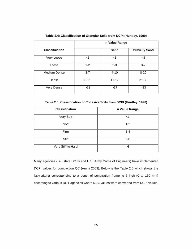
Table 2.4: Classification of Granular Soils from DCPI (Huntley, 1990) ............................ 35

Table 2.5: Classification of Cohesive Soils from DCPI (Huntley, 1990) ........................... 35

Table 2.6: DCP criteria (NDCP) for a penetration of 0 to 6 inch (0 to 150 mm) ............... 36

Table 2.7: Limiting DCPI by MnDOT ................................................................................. 36

Table 2.8: Typical Poisson's Ratio value for Different Types of Materials ........................ 42

Table 2.9: Geogauge and FWD suggested values to characterize base layer ................ 44

Table 3.1: Site Locations of the Pavement Testing for Horseshoe Project, Dallas, TX ... 48

Table 3.2: Summary of the Tests performed in each location .......................................... 56

Table 4.1: Location-wise Resilient Moduli values with Literature Moduli Values (Cement

Stabilized Base Layer) ...................................................................................................... 92

Table 4.2: Location-wise Resilient Moduli values with Literature Moduli Values (Lime

Treated Subgrade Layer) .................................................................................................. 94

Table 4.3: Location-wise Resilient Moduli values with Literature Moduli Values

(Compacted Subgrade Layer) ........................................................................................... 95

Table 4.4: Location-wise UCS values with Literature Values (Cement Stabilized Base

Layer) ................................................................................................................................ 97

Table 4.5: Location-wise Young’s Moduli values measured with Geogauge and TX

Pavement Design Moduli .................................................................................................. 99

1

CHAPTER 1

INTRODUCTION

1.1 Background

United States of America comprises of 4,064,000 miles of public road network throughout

the entire country. The total length of the paved roads is 2,646,000 miles and the rest is

the unpaved roads which is 1,418,000 miles long (Bureau of Transportation Statistics). The

satisfactory performance of the road networks mainly depends on the quality control

measures that were taken during the construction process. In this regard, proper quality

control to ensure the necessary design steps to be performed accordingly needs to be

taken during the construction of the pavement.

The loads coming from the ongoing vehicles mainly pass on to the layers of the pavement

which mainly consists of base course, subbase course and the compacted subgrade

underneath the surface course and the binder course. Hence, proper construction of the

pavement beneath the paved surface is of utmost importance during the construction of

the pavement structure. Proper design life can be ensured if only proper quality control is

maintained throughout the whole construction process.

Several in-situ devices have been used throughout the decades to evaluate the material

properties of the pavement during construction process which can be broken down into

three main major categories (MnDOT):

1. Determination of shear strength:

(i) Dynamic Cone Penetrometer (DCP)

(ii) Rapid Compaction Control Device (RCCD)

2. Determination of Elastic Modulus:

(i) Dynatest Falling Weight Deflectometer (FWD)

(ii) Loadman Portable FWD (PFWD)

2

(iii) PRIMA PFWD

(iv) Humboldt Geogauge

3. Determination of Density:

(i) Sand Cone Method

(ii) Nuclear Density Gauge (NDG)

In the recent decades, popularity of Dynamic Cone Penetrometer and Geogauge are

increasing due to their simplicity in use and less time required to estimate material qualities.

Dynamic Cone Penetrometer has been used by many agencies throughout the years but

the use of Geogauge for assessing the material quality is recent. Dynamic Cone

Penetrometer is a simple hand-held device to measure the in-situ strength of base,

subbase and subgrade and the thickness and location of underlying soil layers and has

been used in geotechnical investigations for a few decades. This equipment can estimate

the strength, pavement condition and variability of granular bases and subgrade soils of

existing pavements.

Geogauge which was formerly known as Soil Stiffness Gauge is a hand-portable gauge

used to measure lift stiffness and soil modulus for compaction process control. Geogauge

measures the impedance at the surface of the soil i.e., the stress imparted to the surface

and the resulting surface velocity as a function of time which provides the stiffness of the

underlying material of the pavement. Few agencies including U.S. Army Corps of

Engineers, Federal Highway Authority (FHWA), Minnesota Department of Transportation

(MnDOT), New York State Department of Transportation (NYSDOT), North Carolina

Department of Transportation (NCDOT) and Texas Department of Transportation (TxDOT)

have recently been using Geogauge in their construction works.

3

1.2 Problem Statement

The Horseshoe Project is a $798 million design-build roadway construction project

undertaken by the Texas Department of Transportation (TxDOT). The project was taken

into account to improve the traffic flow through the heart of the downtown Dallas which

includes construction improvements such as expansion, repaving and addition of new

bridges and roadways along Interstates 30 and 35E and construction of a new signature

bridge named the Margaret McDermott Bridge over I-30. The timeline to complete the

whole project is from April 2013 to summer 2017 which will ensure the improved safety,

increased capacity and improved mobility through the downtown Dallas.

Typically, as a part of the QA/QC program of the horseshoe project, the conventional core

samples are collected to determine the strength and stiffness parameters to assess the

construction quality. However, collecting the core samples followed by laboratory testing is

time consuming and might be expensive. Moreover, the core collection is performed every

few thousand feet and considered that collected core sample is representing the overall

strength of the entire section. However, the strength and stiffness may vary within few feet.

Therefore, adopting the insitu technique as a part of the QA/QC program will provide more

data points which may help to improve the construction quality and compliance. The in-situ

test such as DCP and Geogauge can be performed within the horseshoe project to assess

the construction quality, uniformity, layer stiffness moduli as well as compaction level as a

part of the QA/QC work.

1.3 Objectives

The major objective of this study is to utilize the in-situ test technique such as DCP and

Geogauge to evaluate the construction quality and compliance with the design standard in

different locations of the horseshoe project. The specific objective of the study includes:

4

Perform DCP and Geogauge tests at different location of the Horseshoe project

on monthly basis after placing the base layer.

Determine the layer thickness from DCP Index profile along depth obtained from

Dynamic Cone Penetrometer test.

Assess resilient moduli values and unconfined compressive strength in different

layers of the pavement using Dynamic Cone Penetrometer.

Evaluate the variation of Young’s moduli across the width of the pavement with the

use of Geogauge.

Compare of DCP and Geogauge test results.

Compare DCP and Geogauge test results between current and previous studies.

1.4 Organization

A brief summary of the chapters included in this thesis is presented in the following

paragraphs:

Chapter 1 provides an introduction and presents the problem statement and objectives of

the study that has been conducted under Horseshoe Project.

Chapter 2 presents the background, an overview and use of Dynamic Cone Penetrometer

and Geogauge in the recent research works carried out by different agencies across United

States.

Chapter 3 presents the methodology of the field tests, the layout in which the tests at the

field were carried out and procedures to analyze the data collected from field tests

performed in different locations of Dallas, TX under Horseshoe Project.

5

Chapter 4 describes the analysis results of the in-situ tests performed with Dynamic Cone

Penetrometer, Geogauge and Nuclear Density Gauge and the comparison of the results

obtained from tests performed with the literature.

Chapter 5 discusses the comparison drawn to evaluate the qualitative use of Dynamic

Cone Penetrometer and Geogauge as an in-situ pavement testing technique.

6

CHAPTER 2

LITERATURE REVIEW

2.1 Introduction

This chapter reviews the test devices (i.e., Dynamic Cone Penetrometer and Geogauge)

that were used in this study. This summary contains history, background, working principle,

existing correlations for soil measurements and the current uses of these two devices.

2.2 Dynamic Cone Penetrometer

2.2.1 Background

Efficient construction of pavement as well as its performance evaluation requires a proper

and representative characterization of materials. In geotechnical engineering, in-situ

penetration techniques have become popular and are being widely used to serve this

purpose due to its simplicity and low cost of operation. Two of the most typical in-situ

penetration tests which have been used due to this reason are the Standard Penetration

Test (SPT) and the Cone Penetration Test (CPT). In SPT test, a sampler is driven into the

soil with hammer blow whereas, the principle on which CPT is operated is quasi-static. Due

to its nature of consuming much time during the construction phase, the need of a more

time saving in-situ testing device was realized.

The Dynamic Cone Penetration test (DCP) was first developed by Scala in South Africa as

an in-situ pavement evaluation technique for evaluating pavement layer strength (Scala,

1956). Dynamic Cone Penetrometer (DCP) has been used to measure the in-situ shear

resistance of soil because a soil’s shearing resistance is its ability to withstand load. But a

newer form of the Dynamic Cone Penetrometer was designed by Dr. D. J. van Vuuren with

a 30° cone in 1969. Afterwards, the Transvaal Roads Department in South Africa started

using DCP to investigate road pavement in 1973 (Kleyn, 1975) with a 30° cone tip.

Afterwards the results which were obtained using 30° and 60° cone tip were reported by

7

Kleyn.Kleyn found that when a DCP measurement is plotted against a CBR obtained from

the lab experiments on a log-log graph, the relationship between these two parameters are

linear. Despite giving much effort to find out a way to use the DCP curves as an indicator

of pavement condition, Kleyn was unable to find any pattern that would give any indication

about the pavement condition. Then in 1982, the final conclusion about the Dynamic cone

Penetrometer was drawn by Kleyn after comparing sound pavement sections with failed

pavement sections where he found a minimum strength or suitability for the base course.

It has been extensively used in South Africa, United Kingdom, Australia, New Zealand and

several States in the U.S.A. such as California, Florida, Illinois, Minnesota, Kansas,

Mississippi and Texas for the characterization of the pavement layers and subgrades. The

U. S. Corps of Engineers has also used DCP as an in-situ testing tool. The Dynamic Cone

Penetrometer has been proven as an effective tool in measuring the strength parameter of

the pavement layers and subgrade conditions.

Figure 2.1: Dynamic Cone Penetrometer

California Bearing Ratio (CBR) values for a soil were used as an indicator of shear strength

for the pavement applications in military. CBR is measured with a standardized penetration

shear test and usually performed on laboratory compacted test specimens during the

design phase of the pavement. In these situations to determine the CBR value, destructive

8

test pits were usually dug to determine pavement layer thicknesses and characterization

of subgrade materials. This test was time consuming and impractical during the

construction of the pavement.

The Dynamic Cone Penetration (DCP) is a simple field test method, consumes less time

in practical applications, require less maintenance and a continuous profile of the pavement

layers can be achieved with higher accuracy. Manually driving mechanism is avoided in

the operation of DCP. The greatest advantage of DCP over other in-situ pavement testing

devices is that it can locate the zone of weakness within the pavement easily

2.2.2 Principle

The Dynamic Cone Penetrometer Test is performed by dropping a hammer of a specific

weight from a certain height which constitutes features both of SPT and CPT. The DCP

test is standardized by ASTM D 6951-03. The penetration depth per blow up to a depth

needed is measured thus resembling this to SPT procedures which measures blow count

using the soil sampler. A 60° cone is used to create a cavity during the DCP test instead

of using the split spoon soil sampler, this operation makes it similar to CPT as well. The

principles on which the DCP operates on seem to reduce many of the deficiencies that

occurred during manually getting into the soil.

The Dynamic Cone Penetrometer can provide continuous measurements of the pavement

layers and the underlying subgrade without digging the existing pavement which is

encounters during CBR test [7]. It constitutes an upper fixed travel shaft which is 22.6 inch

(575 mm) long with a 17.6 lbs (8 kg) falling weight which exerts an energy of about 78.5 N

and a lower shaft of 39.4 inch (1000 mm) which contains an anvil and a replaceable cone

with an apex angle of 60° and 0.8 inch (20 mm) diameter. The anvil stops the hammer from

falling further than the standard falling height which ensures a constant driving force of the

cone into the ground. An additional rod which is attached to the lower shaft is used as scale

9

to measure the penetration per blow.The shaft has a smaller diameter than the cone (16

mm) to reduce the skin friction during the penetration of the cone into the soil. A schematic

of the DCP is given below in Figure 2.2.

Figure 2.2: Dynamic Cone Penetrometer Schematic (Source: MnDOT DCP Design)

Few configuration options are available for the DCP in the market for the use which include

changing the mass of the falling weight, type of tip and recording method. The standard

hammer mass is 17.6 lbs (8 kg) but 10.1 lbs (4.6 kg) mass is also available for a weaker

soil. The smaller mass weight can be used on soils with a CBR value up to 80. The bigger

between these two is usually used for the pavement application. The pavement layers are

compacted and requires more energy from the falling weight for the proper penetration to

occur. The tip which is attached to the lower portion of the DCP can be replaceable point

10

or disposable cones. The replaceable point remains for a certain period of time until it

becomes worn out or damaged beyond a certain limit and then it is replaced with a newer

one. On the contrary, the disposable cone remains in the soil after every test. The main

reason behind using disposable cones with the DCP is that it helps to remove the DCP

shaft from the soil after the penetration process is performed.

Performing DCP test requires two persons where one person let the weight fall freely from

a specified height and the other person records the measurement. The lower shaft can

move independently with the scale attached to it for the measurement to be recorded. The

scale stays on the ground surface so that the penetration of the shaft can be measured

with respect to the ground surface. The cone tip is being placed on the surface being tested

at first and afterwards, the test is performed by letting the fall freely. The cone must have

to penetrate a minimum of 25 mm between recorded measurements. Data which are taken

at less than 25 mm penetration increments sometimes results in inaccurate strength

determinations hence, to be avoided. The number of hammer blows between

measurements should be between 1, 2, 3, 5, 10, 20 depending on the cone penetration

rate. The initial reading recorded before any hammer blow is counted as initial penetration

corresponding to blow 0. The falling of the mass is repeated until the desired depth is

reached and the penetration depth for each blow is measured for each hammer drop. The

penetration procedure performed with the DCP is shown in Figure 2.3 (Salgado and Yoon,

2003).

11

Figure 2.3: The Dynamic Cone Penetration (DCP) Test Procedure (Salgado and Yoon, 2003)

While determining the layer thickness, the slope of the curve between number of blows

and depth of penetration (mm/blow) is denoted as the DCP Penetration Index (DCPI). It

can be calculated as (Embacher, 2005):

DCPI = 𝑃(𝑖+1)−𝑃(𝑖)

𝐵(𝑖+1)−𝐵(𝑖)

Where, DCPI = Dynamic Cone Penetration Index (mm/blow)

12

P = Penetration at ith or (i+1)th hammer drops (mm)

B = blow count for ith or (i+1)th hammer drops

A typical plot of DCP test results is presented below in Figure 2.4. The slope of this graph

at any point represents the value of Dynamic Cone Penetration Index (DCPI) in mm/blow

which indicates the amount of resistance the material is exerting towards the cone. The

lower DCPI values indicates a stiffer soil and vice versa.

Figure 2.4: DCPI Profile of a Flexible Pavement (Gudishala, 2004)

13

A standard procedure should be followed while analyzing the data recorded from DCP

measurement for a representative value of penetration per blow. For a specific location, a

representative DCPI value for a certain amount of depth being considered can be obtained

using any of the two methods mentioned below:

Arithmetic Average:

The arithmetic average is obtained using the following equation (Edil and Benson,

2005):

DCPIavg = ΣiN (DCPI)/N

Where, N = Total number of DCPI recorded for a given depth

Weighted Average:

The weighted average is obtained from the following equation (Edil and Benson,

2005):

DCPIwt.avg = 1

𝐻*Σi

N* (DCPIi* Zi)

Where, Z = Penetration Depth per Blow Set

H = Total Penetration Depth

2.2.3 Terminology

From the early stages of the development of DCP, many indices were derived from DCP

data to characterize the pavement layers.

Kleyn et al. defined the DCP Structure Number (DSN) as the number of blows required to

penetrate a layer of material (Kleyn et al., 1982). According to them, DSN of the ith layer,

DSNi, can be defined as the number of blows required to penetrate the layer thickness h i

(mm/inch) at an average PR of DNi (mm/inch) per blow.

DSNi = hi/DNi

14

The pavement DSN was denoted as the number of blows required to penetrate the whole

pavement structure:

DSN = Σ DSNi

The pavement strength balance NDCP was defined as the number of blows required to

penetrate 10 cm (3.9 inch)

Over the past few decades, data taken from DCP measurements have also been

represented in the following chart formats (Kleyn, 1975):

1. The Foundation Balance Graph: A plot of depth over PR with both axes in log scale

which is presented in Figure 2.5.

The DCP Factor: The area enclosed by the foundation balance graph

Figure 2.5: Foundation Balance Graph (Kleyn) (1 inch = 25.4 mm)

15

2. The Strength-Balance Curve (Presented in Figure 2.6: )

Figure 2.6: Strength-Balance Curve (Kleyn) (1 inch = 25.4 mm)

3. The Layer Strength Diagram: The depth in natural numbers and the PR in log scale

4. The DCP Curve: The number of blows needed to reach a certain depth

DCP data have been interpreted in different ways from the beginning of DCP being used

for the pavement characterization. Below are some of the different forms of DCP

measurements which measure the depth of penetration per blow:

i. Penetration Rate (PR)

ii. DCP Number (DN) (Kleyn, 1975)

iii. DCP Index (DI or DCPI) (Harison, 1989)

iv. Blow Number (BN)

In this report, measurement taken from DCP will be denoted as the DCPI.

16

2.2.4 Application Of Dynamic Cone Penetrometer

According to Kleyn, Maree and Savage (1982), Dynamic Cone Penetrometer can be used

in construction projects to evaluate the following:

1. Potentially collapsible soils

2. Construction control

3. Efficiency of compaction

4. Stabilized layers

5. Subgrade moisture content

The MnDOT recommended two applications of DCP as a quality control device:

1. During the compaction of backfill of pavement edge drain trenches.

2. During the compaction of granular base layer.

Each layer of granular base layer requires less than 19 mm per blow (0.75 inches per blow)

to ensure the proper compaction. This DCPI limiting value is valid for freshly compacted

base materials because DCPI value decreases quickly with time and under traffic loading.

MnDOT recommended using other devices along with DCP to ensure proper compaction.

Based on the studies conducted by Siekmeier (1998), MnDOT revised the limiting

penetration rate based on the agreement between the DCPI and percent compaction which

are as follows:

1. 15 mm/blow in the upper 75 mm (3.0 inch)

2. 10 mm/blow at depth between 75 and 150 mm (3 and 6 inch)

3. 5 mm/blow at depth below 150 mm (6 inch)

17

They recommended the following:

(i) The test should be performed consistently and not more than one day after

compaction while the base material is still damp.

(ii) The construction traffic should be distributed uniformly by requiring haul trucks

to vary their path.

(iii) At least two dynamic cone penetrometer tests should be conducted at selected

sites within each 800 cubic meters of constructed base course.

The Wisconsin DOT identified DCP and rolling wheel deflectometer as an effective tool in

identifying weak areas of in-situ subgrade for construction acceptance (Corvetti &

Schabelski, 2001).

Presence of shallow bed rock or less than 3 inch (75 mm) of asphalt concrete layer often

result in misinterpretation of backcalculated moduli from falling weight deflectometer

(FWD). DCP can accurately be used in these kinds of situations where weak subgrade or

base layers can cause large deflections which exceed the calibration limit of the equipment.

A stiffer material results in lower values of DCPI whereas, a soft material provides higher

values of DCPI. The following Figure 2.7 presents the average strength profile of an

existing flexible pavement.

Figure 2.7: Average Strength Profile of a Flexible Pavement

18

Soil layer thickness can also be determined from the change in slope of the depth vs the

profile of the accumulated blows. Livneh (1987) matched the layer thickness obtained from

the measurements taken with the DCP to the thickness obtained from the test pits and

hence, concluded that the DCP test is reliable to determine the layer thickness for

evaluating any project.

2.2.5 Factors Affecting DCP Measurements

2.2.5.1 Material Effects

Many researchers have conducted research activities to evaluate the factors that might

affect the measurements taken with the Dynamic Cone Penetrometer which include soil

type, gradation, moisture content, density, plasticity and maximum aggregate size.

Kleyn& Savage (1982) concluded that the plasticity, density, moisture content and

gradation influentially affect the measurements taken with the DCP. According to Hassan

(1996), DCP measurements are significantly affected by moisture content, AASHTO soil

classification, confining pressures and dry density for fine grained soils whereas, George

(2000) suggested that the DCP data to be affected by the maximum aggregate size and

the coefficient of uniformity. Harison (1987) observed the trend between DCPI, moisture

content and dry unit weight which is presented below in the Figure 2.8.

19

Figure 2.8: Trend among the trends obtained from Laboratory results (Harison, 1987)

20

2.2.5.2 Vertical Confinement Effects

The effect of vertical confinement on strength of soil obtained from the measurement taken

with the DCP was studied by Livneh et al. (1995) and no effect of vertical confinement by

rigid pavement structure or by upper cohesive layers on the DCP data of lower cohesive

subgrade layers have been observed by them. However, vertical confinement effect by the

upper asphaltic layers on the DCP data of the granular pavement layers has been

observed. This influence might be occurred because of the friction developed in the DCP

shaft by tilted penetration or by a collapse of the granular material on the shaft surface

during penetration.

2.2.5.3 Side Friction Effect

Side friction often generated while penetrating is mainly due to the non-vertical penetration

of DCP shaft in to the soil. It can also be generated while penetration occurs in a collapsible

granular material. However, the amount side friction generated in cohesive soils is often

small. According to Livneh (2000), a correction factor can be used to correct the DCP value

for the side friction effect.

2.2.6 Existing Correlations Between DCP And California Bearing Ratio (CBR)

Penetration rates of the cone of Dynamic Cone Penetrometer into the base, sub-base and

subgrade soil can be converted into CBR. Assessing the structural properties of a

pavement layers often requires the DCP values to be converted into CBR. Different

correlations were suggested between the DCPI (mm/blow) and CBR values.

21

Based on the previously performed researches, it has been observed that the relationship

between DCPI and CBR values are often one of the following forms presented below:

Log-Log Equation: Log (CBR) = a + b (Log DCPI)

Where, CBR = California Bearing Ratio

DCPI = Dynamic Cone Penetration Index

a = constant ranging from 1.55 to 3.93

b = constant ranging from -0.55 to -1.65

Inverse Equation: CBR = D (DCPI) E + F

Where, D, E, F = Regression Constants

U.S. Army Corps of Engineers developed a relation between DCPI and CBR based on a

wide range of granular and cohesive materials which was adapted by many researchers

[12].

Log CBR = 2.465 – 1.12 (Log DCPI)

Or, CBR = 292

𝐷𝐶𝑃𝐼^1.12

This correlation can be presented by the chart presented below:

Figure 2.9: Correlation chart between CBR vs DCPI

22

Based on the field CBR and the average of three measurements taken with the DCP within

an area with a radius of less than 1 ft (0.3 m), the North Carolina Department of

Transportation (NCDOT) (Wu, 1987) suggested the following relationship:

Log (CBR) 2.64 – 1.08 (Log DCPI)

Or, CBR = 435

𝑃𝑅^1.08 (R2=0.79)

Figure 2.10: Comparison of Different CBR-Moduli Relationships (Wu and Sargand, 2007)

The study conducted by U.S. Army Corps of Engineers was based on the CBR values

obtained from the lab experiments and the CBR values obtained by NCDOT were from

field. It has been observed that the CBR values obtained from field is twice than the values

obtained from lab experiments. The results of these two experiments were in good

agreements, Webster et al. (1994) refined this equation and suggested correlations

suitable for different soil types.

CBR = 1

(0.002871∗𝐷𝐶𝑃𝐼) (for high plasticity clay soil (CH))

CBR = 1

(0.017019∗𝐷𝐶𝑃𝐼)^2 (for low plasticity clay soil (CL))

23

After performing DCP tests on 2000 sample of pavement materials in standard molds,

Kleyn [8] recommended the following equation. He found out that the measurements taken

from the DCP varied in a way as the CBR varies with the moisture content. According to

him, DCP-CBR relationship was independent of moisture content.

Log CBR = 2.62 – 1.27 (log DCPI)

Smith and Pratt suggested the following correlation based on a field study [9]:

Log CBR = 2.56 – 1.15 (log DCPI)

Observing the small difference between the two relationships above, Livneh et al. (1994)

proposed the following equation as the best correlation:

Log CBR = 2.46 – 1.12 Log (DCPI)

Using a wide range of undisturbed and compacted fine-grained soil samples with or without

saturation, Livneh and Ishia developed a correlation between DCPI and the in-situ CBR.

Compacted granular soils were tested in flexible molds with variable controlled lateral

pressures. The following relationship was developed by them [10]:

Log CBR = 2.2 – 0.71 (Log DCPI)1.5

Livneh, M. (1989) developed the following relationship based on field and laboratory tests:

Log CBR = 2.14 – 0.69 (Log DCPI)1.5

The following relationships were developed by Harrison for different soils [11]. According

to him, soaking process has an insignificant effect on the CBR-DCP relationship

Log CBR = 2.56 – 1.16 Log (DCPI) (clayey-like soil where PR> 10 mm/blow)

Log CBR = 2.70 – 1.12 Log (DCPI) (granular soil where PR<10 mm/blow)

According to tests conducted by Coonse (1999) on piedmont residual soils, he developed

an empirical relationship between CBR and DCP [12]. He concluded that the CBR-DCP

relationship is independent of moisture content, dry density and soaking.

Log (CBR) = 2.53 - 1.14 (Log DCPI)

24

Based on the tests performed on aggregate base course, Ese et al, (1994) developed the

following correlation:

Log (CBR) = 2.44 – 1.07 (Log DCPI)

Ese (Norwegian Road Research Laboratory) correlated field measurements taken with the

DCP with lab CBR values. He suggested the following relationship:

Log (CBRlab) = 2.438 – 1.65 (Log DCPIfield)

Where, CBRlab= CBR values obtained from the lab experiments

CBRfield= CBR values obtained in the field

Webster et al. (1992) suggested the following relationship based on tests performed on

various types of soil.

Log (CBR) = 2.46 – 1.15 (Log DCPI)

Based on the coupled contribution of the subgrade and the aggregate base course

material, Gabr et al. (2000) conducted a regression analysis to develop a relationship

between CBR and DCP and afterwards, the model was validated using data set from four

test sites.

Log (CBR) = 1.55 – 0.55 (Log DCPI) (R2=0.82)

Lee et al. (2014) suggested a correlation between these two parameters based on

laboratory experiments on weathered sandy soil (SP, SM and SW-SM) in Korea with high

R2 value.

Log (CBR) = 3.93 – 1.47 (Log DCPI) (R2=0.93)

Abu-Farsakh et al. (2004) developed a relationship between the CBR value and DCPI

which is given below:

CBR = 5.1

𝐷𝐶𝑃𝐼0.2−1.41 (R2=0.93)

Many correlations have been developed by the researchers and organizations around the

world. Based on the results obtained from different sources, the equation developed by

25

U.S. Army Corps of Engineers was selected as the best correlation among all the equations

and has been adopted.

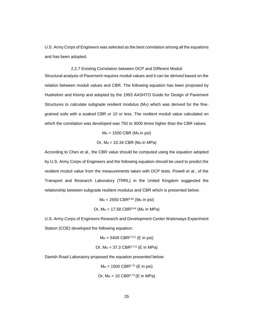
2.2.7 Existing Correlation between DCP and Different Moduli

Structural analysis of Pavement requires moduli values and it can be derived based on the

relation between moduli values and CBR. The following equation has been proposed by

Huekelom and Klomp and adopted by the 1993 AASHTO Guide for Design of Pavement

Structures to calculate subgrade resilient modulus (MR) which was derived for the fine-

grained soils with a soaked CBR or 10 or less. The resilient moduli value calculated on

which the correlation was developed was 750 to 3000 times higher than the CBR values.

MR = 1500 CBR (MR in psi)

Or, MR = 10.34 CBR (MR in MPa)

According to Chen et al., the CBR value should be computed using the equation adopted

by U.S. Army Corps of Engineers and the following equation should be used to predict the

resilient moduli value from the measurements taken with DCP tests. Powell et al., of the

Transport and Research Laboratory (TRRL) in the United Kingdom suggested the

relationship between subgrade resilient modulus and CBR which is presented below:

MR = 2550 CBR0.64 (MR in psi)

Or, MR = 17.58 CBR0.64 (MR in MPa)

U.S. Army Corps of Engineers Research and Development Center Waterways Experiment

Station (COE) developed the following equation:

MR = 5409 CBR0.711 (E in psi)

Or, MR = 37.3 CBR0.711 (E in MPa)

Danish Road Laboratory proposed the equation presented below:

MR = 1500 CBR0.73 (E in psi)

Or, MR = 10 CBR0.73 (E in MPa)

26

The moduli values computed from the above mentioned formulae vary significantly which

is presented below in the chart.

A study was conducted by George et al. using the laboratory resilient modulus to develop

a model from DCP parameters. Two different models were suggested by them which are

given below:

1. Fine-grained Soils:

MR = a0 (DCPI)a1 (γdra2 + (LL/wc)a3)

Where , MR = Resilient Modulus (MPa)

DCPI = Dynamic Cone Penetration Index (mm/blow)

wc = Actual moisture content (%)

γdr = Density Ratio, Filed Density/Maximum Dry Density

LL = Liquid Limit (%)

a0, a1, a2, a3 = Regression Coefficients

2. Coarse-grained Soils:

MR = a0 (DCPI/Log cu)a1 (wcra2 + γdr

a3)

Where, MR = Resilient Modulus (MPa)


cu = Coefficient of uniformity

wcr = Moisture Ration, Field Moisture/Optimum Moisture Content

γdr = Density Ratio, Filed Density/Maximum Dry Density

a0, a1, a2, a3 = Regression Coefficients

27

A regression model was developed by Hassan for fine-grained soils at optimum moisture

content.

MR = 7013.065 – 2040.783 ln (DCPI)

Where, MR= Resilient Modulus in psi

DCPI = Dynamic Cone Penetration Index in inches/blow

According to Pen, the following two relationships between subgrade elastic modulus (Es)

and DCPI can be defined as:

Log (Es) = 3.25 – 0.89 Log (DCPI)

Log (Es) = 3.652 – 1.17 Log (DCPI)

Where, Es = Subgrade Elastic Modulus (MPa)


Chua related cone apex angle to a model to interpret the results of DCP to determine the

elastic modulus using DCPI where the value of elastic modulus depends on the principal

stress differences at failure (2τ0).

Log (Es) = B – 0.4 Log (DCPI)

Where, Es = Elastic Modulus (MPa)

B = constant whose value depends on 2τ0. Different conditions of 2τ0 and B for various

types of soil are given in the table below:

Table 2.1: Values of B and 2τ0 for Different Types of Soil

Soil Type 2τ0 B

Plastic Clay 25 2.22

Clayey Soil 50 2.44

Silty Soil 75 2.53

Sandy Soil 150 2.63

28

A regression analysis was conducted by Chen et al. between the FWD back-calculated

resilient modulus and DCPI and the following relationship was proposed:

MFWD = 338 (DCPI)-0.39 (for 10 mm/blow < DCPI < 60 mm/blow)

Where, MFWD = FWD back-calculated resilient modulus (MPa)

Pandey et al. developed a correlation between DCPI and backcalculated modulus from

falling weight deflectometer, MFWD, which is given below:

MFWD = 357.87 (DCPI)-0.6445

FWD deflection data and DCPI were used byJianzhou et al. to predict the backcalculated

subgrade modulus from measurements taken with DCP.

EFWD = 338 (DCPI)-0.39

Where, EFWD = Backcalculated Elastic Modulus (MPa)

And DCPI is in mm/blow

The correlation developed by Abu-Farsakh et al. (2004)between the DCPI and the back-

calculated modulus obtained from FWD is given below:

ln (MFWD) = 2.35 + 5.21

ln(𝐷𝐶𝑃𝐼) (R2=0.91)

De Beer suggested a relationship between elastic modulus of soil (Es) and DCPI:

Log (Es) = 3.05 – 1.07 Log (DCPI)

Chai et al. suggested the following model based on the DCP test and CBR-DCPI

relationships which was developed in Malaysia during 1987 to calculate the subgrade

elastic modulus.

E = 17.6 (269/DCPI)0.64

Where, E = Subgrade elastic modulus in MN/m2

DCPI = Dynamic Cone Penetration Index in blows/300 mm penetration

29

Chai et al. proposed a relationship correlating the backcalculated elastic modulus to DCPI

which is given below:

E = 2224 (DCPI)-0.996

Where, E = Backcalculated Subgrade Elastic Modulus (MN/m2)

Based on the DCPI of a large DCP with a 51 mm diameter cone and the elastic modulus

of unbound aggregates and natural granular soils back-calculated from plate load tests

(EPLT) (in MPa), Konard and Lachance also suggested a relationship which is as follows:

Log (EPLT) = -0.88405 Log (DCPI) + 2.90625

Abu-Farsakh et al. (2004) conducted a detailed experimental program to assess the

accuracy of in-situ test methods which include DCP, Static Plate Load test, Falling Weight

Deflectometer test and CBR test data which were collected in the field. The correlations

between the DCPI and both the initial modulus and the reloading stiffness of SPLT are

given below:

Relation with Initial Modulus obtained from Plate Load Test in field:

Ei = 17421.2

𝑃𝑅2.05+62.53 – 5.71 (Ei in MPa)

Or, Ei = 2526.7

𝑃𝑅2.05+62.53 – 0.828 (Ei in ksi) (R2=0.94)

Relation with Reloading Modulus obtained from Plate Load Test in field:

ER= 5142.61

𝐷𝐶𝑃𝐼1.57−14.8 – 3.49 (ER in MPa)

Or, ER= 745.87.

𝐷𝐶𝑃𝐼1.57−14.8 – 0.506 (ER in MPa) (R2=0.95)

Based on the laboratory experiments conducted by Mohammadi et al. (2008), two different

relationships between DCPI and Initial modulus (EPLT(i)) and Reloading stiffness modulus

(EPLT(R2)) were developed which are given below:

(i) EPLT(i) = 55.033

𝐷𝐶𝑃𝐼0.54 (R2=0.83) (E in MPa)

30

EPLT(R2) =

53.73

𝐷𝐶𝑃𝐼0.74 (R2=0.94) (E in MPa)

(ii) EPLT(R2) = 0.16 (EPLT(i))1.49 (R2=0.94) (E in MPa)

Chen et al. (2005) developed a correlation using the DCP test results to determine the

Young’s modulus:

E = 78.05 (DCPI)-0.6645 (E in ksi)

Or, E = 537.76 (DCPI)-0.6645 (E in MPa)

R2 value was found to be 0.855.

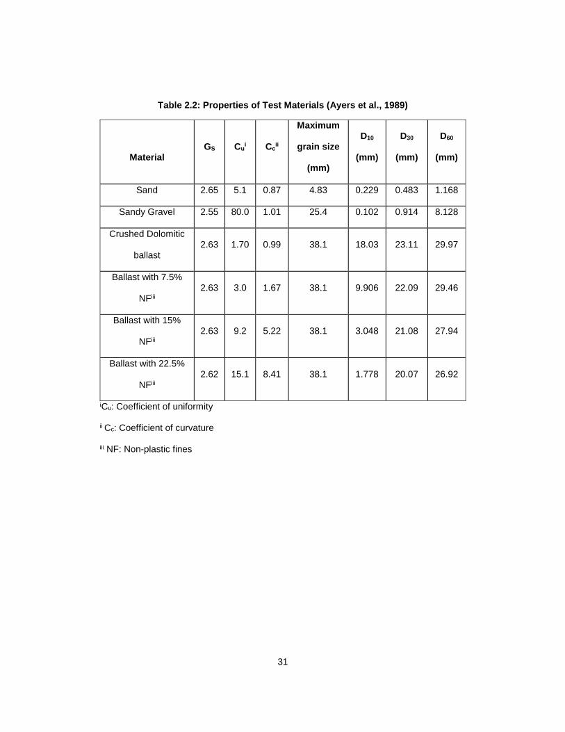
2.2.8 Existing Correlation Between DCP And Shear Strength Of Soil

Ayers et al. (1989) developed equations based on the laboratory tests performed on

different base material for various confining pressures to evaluate the efficiency of the DCP

for determining the shear strength of granular material. Laboratory DCP and triaxial tests

were performed on sand, dense-graded sandy gravel, crushed dolomite ballast, and ballast

with varying amounts of non-plastic crushed dolomitic fines to obtain the DCPI and shear

strength to develop correlations which take form as:

DS = A – B (DCPI)

Where, DS = Shear Strength of soil

DCPI = Dynamic Cone Penetration Index

A, B = Regression Coefficients

The material properties and the correlations between DCPI and shear strength of the above

mentioned materials and confining stress level are given in the Table 2.2 and Table 2.3.

31

Table 2.2: Properties of Test Materials (Ayers et al., 1989)

Material GS Cu

i Ccii

Maximum

grain size

(mm)

D10

(mm)

D30

(mm)

D60

(mm)

Sand 2.65 5.1 0.87 4.83 0.229 0.483 1.168

Sandy Gravel 2.55 80.0 1.01 25.4 0.102 0.914 8.128

Crushed Dolomitic

ballast 2.63 1.70 0.99 38.1 18.03 23.11 29.97

Ballast with 7.5%

NFiii

2.63 3.0 1.67 38.1 9.906 22.09 29.46

Ballast with 15%

NFiii

2.63 9.2 5.22 38.1 3.048 21.08 27.94

Ballast with 22.5%

NFiii

2.62 15.1 8.41 38.1 1.778 20.07 26.92

iCu: Coefficient of uniformity

ii Cc: Coefficient of curvature

iii NF: Non-plastic fines

32

Table 2.3: Correlation between DCPI and Shear Strength (Ayers et al. 1989)

Material Confining Stress (kPa) Correlation

Sand

34.5 DS = 41.3 – 12.8 (DCPI)

103.4 DS = 100.4 – 23.4 (DCPI)

206.9 DS = 149.6 – 12.7 (DCPI)

Sandy Gravel

34.5 DS = 51.3 – 13.6 (DCPI)

103.4 DS = 62.9 – 3.6 (DCPI)

206.9 DS = 90.7 -5.8 (DCPI)

Crushed Dolomitic Ballast

34.5 DS = 64.1 – 13.3 (DCPI)

103.4 DS = 139.0 – 40.6 (DCPI)

206.9 DS = 166.3 – 16.2 (DCPI)

Ballast with 7.5% NF

34.5 DS = 87.2 – 78.7 (DCPI)

103.4 DS = 216.1 – 213.9 (DCPI)

206.9 DS = 282.1 – 233.2 (DCPI)

Ballast with 15% NF

34.5 DS = 47.5 – 0.45 (DCPI)

103.4 DS = 184.2 – 215.5 (DCPI)

206.9 DS = 206.4 – 135.7 (DCPI)

Ballast with 22.5% NF

34.5 DS = 49.7 – 23.1 (DCPI)

103.4 DS = 133.1 – 68.6 (DCPI)

206.9 DS = 192.1 - 95.7 (DCPI)

33

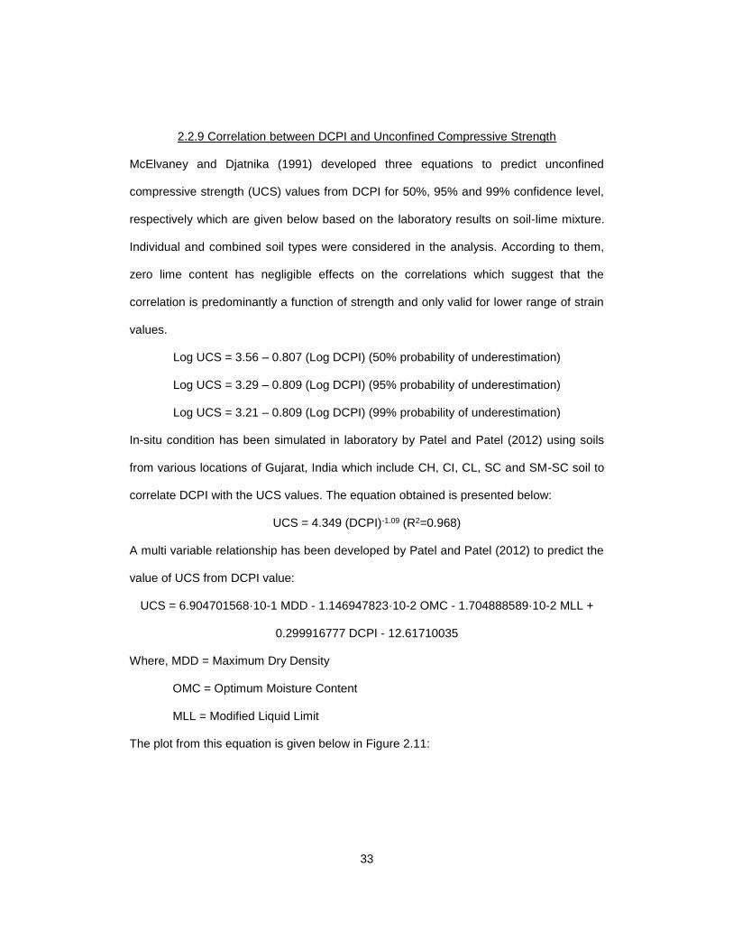
2.2.9 Correlation between DCPI and Unconfined Compressive Strength

McElvaney and Djatnika (1991) developed three equations to predict unconfined

compressive strength (UCS) values from DCPI for 50%, 95% and 99% confidence level,

respectively which are given below based on the laboratory results on soil-lime mixture.

Individual and combined soil types were considered in the analysis. According to them,

zero lime content has negligible effects on the correlations which suggest that the

correlation is predominantly a function of strength and only valid for lower range of strain

values.

Log UCS = 3.56 – 0.807 (Log DCPI) (50% probability of underestimation)



In-situ condition has been simulated in laboratory by Patel and Patel (2012) using soils

from various locations of Gujarat, India which include CH, CI, CL, SC and SM-SC soil to

correlate DCPI with the UCS values. The equation obtained is presented below:

UCS = 4.349 (DCPI)-1.09 (R2=0.968)

A multi variable relationship has been developed by Patel and Patel (2012) to predict the

value of UCS from DCPI value:

UCS = 6.904701568·10-1 MDD - 1.146947823·10-2 OMC - 1.704888589·10-2 MLL +

0.299916777 DCPI - 12.61710035

Where, MDD = Maximum Dry Density

OMC = Optimum Moisture Content

MLL = Modified Liquid Limit

The plot from this equation is given below in Figure 2.11:

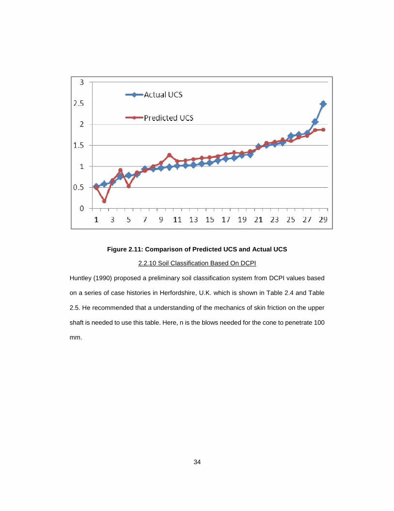
34

Figure 2.11: Comparison of Predicted UCS and Actual UCS

2.2.10 Soil Classification Based On DCPI

Huntley (1990) proposed a preliminary soil classification system from DCPI values based

on a series of case histories in Herfordshire, U.K. which is shown in Table 2.4 and Table

2.5. He recommended that a understanding of the mechanics of skin friction on the upper

shaft is needed to use this table. Here, n is the blows needed for the cone to penetrate 100

mm.

35

Table 2.4: Classification of Granular Soils from DCPI (Huntley, 1990)

Classificaiton

n Value Range

Sand Gravelly Sand

Very Loose <1 <1 <3

Loose 1-2 2-3 3-7

Medium Dense 3-7 4-10 8-20

Dense 8-11 11-17 21-33

Very Dense >11 >17 >33

Table 2.5: Classification of Cohesive Soils from DCPI (Huntley, 1990)

Classification n Value Range

Very Soft <1

Soft 1-2

Firm 3-4

Stiff 5-8

Very Stiff to Hard >8

Many agencies (i.e., state DOTs and U.S. Army Corps of Engineers) have implemented

DCPI values for compaction QC (Amini 2003). Below is the Table 2.6 which shows the

NDCPcriteria corresponding to a depth of penetration fromo to 6 inch (0 to 150 mm)

according to various DOT agencies where NDCP values were converted from DCPI values.

36

Table 2.6: DCP criteria (NDCP) for a penetration of 0 to 6 inch (0 to 150 mm)

Materials ILDOT Iowa DOT MnDot NCDOT

Frictional Soil

6.1i

3.4~4.4ii 12.5iii

4.0iv

Cohesive

Soil

Silt

3.8~4.4ii

6.0iii Clay

iDCP blow counts associated with a CBR of 8

ii Iowa DOT classified the soil either “suitable soil” or “unsuitable soil” in each group of

soil. The values show the ranges of it (Larsen et al., 2007)

iii The criteria of frictional soil apply for “granular” base layer, MnDOT recorded NDCP

values only for blow counts that higher than two (Burnham, 1997)

iv DCP blow counts associated with a CBR of 8 (Gabr et al., 2000)

MnDOT is one of the first states which have been using DCP from 1991 as a tool to

evaluate the strength and uniformity of highway structures. MnDOT defined limiting DCPI

values for each particular subgrade soil and base type after performing more than 700 DCP

tests on Minnesota Road Research project which is presented in Table 2.7. This table was

developed based on the assumption of the presence of adequate confinement near the

testing surface and certainly do not cover all types of materials. It has been suggested by

MnDOT that there is scope to extend the table for other types of base materials.

Table 2.7: Limiting DCPI by MnDOT

Material Limiting DCPI (mm/blow)

Silty/Clay Subgrade <25

Select Granular Subgrade <7

Class 3 Special Gradation Granular Base Materials <5

37

2.3 Soil Stiffness Gauge (Geogauge)

2.3.1 Introduction

Soil Stiffness Gauge measures the in-place stiffness of compacted soil. It is a QC/QA field

tool that measures the uniformity of unbound pavement layers by measuring the variability

in stiffness throughout a structure. Irregularities during the construction process can easily

be detected with the Geogauge. [1]

The technology on which Geogauge operates was first developed by the defense industry

for detecting land mines. The collaboration between Bolts, Beranek, and Newman of

Cambridge, MA, CAN consulting Engineers of Minneapolis, MN, and Humboldt came up

with the product Humboldt Stiffness Gauge which is currently known as Geogauge

presented in Figure 2.12.

Figure 2.12: Geogauge

Geogauge weighs about 22 lbs (10 kilograms) without its case and about 34 lbs (15.5

kilograms) with its case, it has a diameter of 11 inch (280 mm) and a height of 10 inch (254

mm). The carrying case has a dimension of 18.5 inch (470 mm) x 16.5 inch (419 mm) x 13

inch (330 mm). Six D-cell batteries powers the operation of the Geogauge which cover

almost 1000 to 1500 measurements. An annular ring connects the soil with the Geogauge

38

and it has an outside diameter of 4.50 inch (114 mm), an inside diameter of 3.50 inch (89

mm) and a thickness of 0.5 inch (13 mm).

2.3.2 Principle of Operation

The principle of Geogauge is to measure the impedance at the surface of the soil by

measuring the stress imparted to the surface and the resulting surface velocity as a

function of time. It is an effective portable device that can measure the in-situ stiffness of

compacted layers rapidly by imparting small dynamic force to the soil through a ring-

shaped foot at 25 steady state frequencies between 100 and 196 Hz. The displacement it

imparts to the soil layer is less than 0.00005 inch (1.27 x 10 -6 m). According to a laboratory

study conducted by Sawangsuriya et al. (2001), the force generated by the Geogauge is 9

N. The stiffness is determined at each frequency and the average of the 25 measurements

is displayed on the screen. The Stiffness is calculated using the following equation:

K= 𝑃

𝛿

Where, K = Stiffness measured with the Geogauge (MN/m)

P= Applied Force

δ= Deflection imparted by the Geogauge

The shaker of the Geogauge applies a force and this force is transferred to the ground

which is measured by differential displacement across the flexible plate by two velocity

sensors which is presented in Figure 2.13.

39

The expression is as follows:

Fdr= Kflex*(X2 – X1) = Kflex*(V2 – V1)

Where, Fdr= Force applied by Shaker

Kflex= Stiffness of the Flexible Plate

X1 = Displacement at Rigid Plate

X2 = Displacement at Flexible Plate

V1= Velocity at Rigid Plate

V2= Velocity at Flexible Plate

Figure 2.13: Schematic of Geogauge (Humboldt, 1998)

Previously conducted studies based on both finite element analyses and experimental

studies indicated that the Geogauge has an influence radius which covers a range from 9

inch to 12 inch (220 mm to 310 mm).

40

2.3.3 Geogauge Stiffness And Moduli Calculation

The static stiffness, K, of a rigid annular ring on a linear elastic, homogeneous and isotropic

half space has the following functional form (Egorov, 1965):

K = 𝐸∗𝑅

(1−𝑣2)∗𝜔(𝑛)

Where, E= Modulus of Elasticity

𝑣 = Poisson’s Ratio

R = Outside Radius of the Annular ring (2.25 inch)

ω(n) = a function of the ratio of the inside diameter and the outside diameter of the

annular ring.

where, n= 𝑟(𝑖𝑛)

𝑟(𝑜𝑢𝑡) = Radius Ratio of the ring

For the ring geometry of the Geogauge, the parameter ω(n) is equal to 0.565. So,

K = 1.77∗𝑅∗𝐸

(1−𝑣^2 )


E= Modulus of Elasticity

𝑣 = Poisson’s Ratio


According to Lenke et al. (2003), the equations which were used as a principle of operation

of the Geogauge is based on the assumption of infinite elastic half space. This assumption

is violated in the pavement application because pavement sections consist of several finite

thick layers which are made up of material with different strength properties.

The process of measurement takes about 75 seconds as a whole which plays a vital role

to portray the vital role during QC/QA process. The stiffness, K can then be converted into

elastic modulus, E, of soil using the equation proposed by CNA Consulting Engineers:

E= K∗(1−𝑣^2 )

1.77∗𝑅

41

Where, E= Elastic Stiffness Modulus (MPa)

K= Stiffness measured with Geogauge (MN/m)

𝑣= Poisson’s ratio (assumed)

R= Radius of the Geogauge (2.25 inch)

Using the assumed Poisson’s ratio, 𝑣, the shear modulus, G, can also be calculated using

the following equation:

G= 𝑃∗(1−𝑣)

3.54∗𝑅∗𝛿

Where, P= Applied Load

R= Outer Radius of Annular Ring

δ= Induced Surface Deflection

𝑣= Poisson’s ratio (assumed)

Poisson’s ratio has to be assumed to measure stiffness with the Geogauge. For a

Poisson’s ratio of 0.35, a factor of approximately 8.67 can convert the Geogauge Stiffness

(MN/m) to a Stiffness Modulus (MPa). The Geogauge manufacturer (Humboldt)

recommends that Geogauge should be used up to 70 MN/m while measuring layer stiffness

and up to 610 MPa while measuring in-situ moduli value. According to a study conducted

by Chen et al., (2000), it is recommended that Geogauge should be used only up to 23

MN/m and the reason behind this is that the Geogauge may lose accuracy when measuring

stiffness greater than 23 MN/m.

42

Poisson’s Ratio for different materials are shown in Table 2.8.

Table 2.8: Typical Poisson's Ratio value for Different Types of Materials

Material Range Typical Value

Portland Cement Concrete 0.15-0.2 0.15

Untreated Granular

Materials 0.3-0.4 0.35

Cement treated Granular

Materials 0.1-0.2 0.15

Cement treated fine-

grained soils 0.15-0.35 0.25

Lime Stabilized Materials 0.1-0.25 0.2

Lime-Flyash Mixtures 0.1-0.15 0.15

Dense Sand 0.2-0.4 0.35

Fine grained Soil 0.3-0.45 0.4

Saturated Soft Soil 0.4-0.5 0.45

2.3.4 Geogauge Application

Portability, simplicity and less time of operation give Geogauge its main advantage over

other in-situ testing devices. It can measure the in-situ stiffness of compacted soil at a rate

of about one test per 1.25 minute and thus enabling it as a great tool for in-situ testing.

Maintaining uniformity in paving application is of great importance and the mean stiffness

of each layer plays a vital role on how the pavement fatigues, the lifetime of the pavement

and the maintenance procedures. Geogauge paves the way to quick data collection and of

large volume.

43

Non-uniform compaction during earthworks can cause premature failure and non-uniform

structural stiffness is one of the indicators of these effects. Geogauge can easily detect the

non-uniformities of earthworks while revealing voids and discontinuities in the material.

Non-destructive way of testing gives Geogauge the edge over other in-situ testing devices.

Some cases require repeated measurements at the same location over time to satisfy the

design and due to its non-destructive mode of operation, Geogauge can take numerous

measurements at a single location. Geogauge can also be used to ensure satisfactory

performance of pavement and if not, proper maintenance measures can be taken.

Measurement of density is one of main parameters in inspection of materials and

structures. Geogauge can replace the conventional time-consuming devices. It provides a

specific value within a short period of time.

2.3.5 Factors Affecting Geogauge Measurement

According to various studies, it has been observed that the density, moisture content,

boundary conditions and stiffness of underlying layers all affect the Geogauge

measurements.

2.3.6 Correlation Between Geogauge And Resilient Modulus

No attempt has been taken to correlate the Geogauge modulus to resilient modulus

measured in laboratory. But a comparison study between resilient modulus measured in

laboratory and Geogauge modulus measured in the field has been conducted [3][4].

According to Chen et al., the base moduli measured with the FWD are higher than those

measured with the Geogauge [5]. Chen et al. suggested that a general relationship exists

between the Geogauge stiffness and the FWD back-calculated modulus, MFWD:

MFWD = 37.65 HSG – 261.96

Where, MFWD = Moduli measured with FWD (MPa)

HSG = Stiffness measured with Geogauge (MN/m)

44

According to them, the quality of the base layers can be classified by FWD or Geogauge

measurements which are provided in Table 2.9 below:

Table 2.9: Geogauge and FWD suggested values to characterize base layer

Base Quality E(MPa) (Geogauge) K (MN/m)

(Geogauge) MFWD (MPa)

Weak <87 <10 <140

Good 156-209 18-24 310-450

Excellent >261 >30 >700

CNA Consulting Engineers conducted a number of field test to compare the modulus

measured with the Quasi-Static Plate Load Test (QSPLT) with the Stiffness Modulus

measured with the Geogauge. The results indicate that reloading elastic modulus obtained

from QSPLT are similar to the Stiffness Modulus obtained from Geogauge. However,

stiffness modulus measured with Geogauge is nearly 7 times higher than the initial loading

modulus. From the results, it can be observed that the Geogauge stiffness modulus

correlates better with initial modulus than with the reloading and unloading modulus

obtained from QSPLT (Petersen et al., 2002)

E(QPLT)R = 0.8962 (EG) + 25.9 (R2 = 0.23)

E(QPLT)u = 0.6158(EG) + 10.3 (R2 = 0.27)

E(QPLT)i = 0.3388(EG) + 84.7 (R2 = 0.66)

Where, E(QPLT)R = Reloading Modulus obtained from QSPLT

E(QPLT)u = Unloading Modulus obtained from QSPLT

E(QPLT)I = Initial Modulus obtained from QSPLT

EG = Stiffness Modulus obtained from Geogauge

45

Wu et al. [6] proposed the following equation correlating the back calculated resilient

modulus from FWD to Geogauge Stiffness.

MR = 22.69 e0.12*KSSG

Where, MR = Resilient Modulus obtained from FWD (MPa)

KSSG = Stiffness obtained from Geogauge (MN/m)

According to a study conducted by Gudishala, a correlation between Resilient Modulus

and Stiffness Modulus obtained from Geogauge was developed for cohesive soil which is

as follows:

MR = 86.7 * {𝐸(𝐺𝑒𝑜)}^0.3

𝑤 + 2.2γd (R2=0.67)


E(Geo) = Modulus obtained from Geogauge (MPa)

w = measured Water Content (%)

γd= measured Dry Density (KN/m3)

Another model was developed to predict resilient modulus from the moduli values obtained

from Geogauge which was applicable for granular soils and it is as follows:

MR = 20.3 * (EGeo)0.54(R2=0.83)


E(Geo) = Modulus obtained from Geogauge (MPa)

He concluded that the resilient modulus of both cohesive and granular materials is stress

dependent and is affected by physical properties of the material. However, according to

him, models to predict the resilient modulus of granular materials are independent of soil

properties.

Farsakh et al. (2004) conducted a study where potential of three in-situ testing devices

(DCP, Geogauge, LFWD) was evaluated. A model was developed between the Geogauge

data obtained both from laboratory and field with the Plate Load Test data and it has been

46

recommended to adopt the correlation which has been developed using field data to

provide a better correlation.

EPLT(i) = -75.58 + 1.62*EG (R2=0.87)

EPLT(R2) = -65.37 + 1.50*EG (R2=0.90)

Where, EG = Stiffness Modulus obtained from Geogauge

EPLT(i) = Initial Modulus obtained from PLT

EPLT(R2) = Reloading Modulus obtained from PLT

Regression analysis was conducted to develop a model relating Geogauge stiffness

modulus to FWD back-calculated resilient moduli, MFWD.

MFWD = -20.07 + 1.17*EG (R2=0.81)

Where, MFWD = FWD back-calculated Modulus

EG = Stiffness Modulus obtained from Geogauge

During the same study, the Geogauge data based both on the laboratory experiments and

field testing were used to develop a model between Stiffness Modulus obtained from

Geogauge, EG, and CBR value and the correlation based on the field data provided better

correlation between these two parameters which is presented below:

CBR = 0.00392*(EG)2 -5.75 (R2=0.84)

Lee et al. (2014) performed laboratory tests using Soil Stiffness Gauge (SSG), Dynamic

Cone Penetrometer (DCP) and Plate Load Test (PLT) and California Bearing Ratio (CBR)

Test on three uncemented soil groups ( poorly graded sand (SP), silty sand (SM), and well-

graded sand with silt (SW-SM) and and conducted regression analysis to develop possible

correlation of moduli values obtained from Geogauge with moduli values obtained from

PLT and dry unit weight which are presented below:

EPLT = 0.59*ESSG (R2=0.65)

47

𝛾𝑑 = 20.6∗(

𝐷50

𝑒)∗ESSG

(𝐷50

𝑒)∗ESSG+20.6

(R2=0.88)

Where, EPLT = Moduli obtained from PLT (MPa)

ESSG = Moduli obtained from Geogauge (MPa)

𝛾𝑑 = Dry Unit Weight (KN/m3)

e = Void Ratio

Chen et al. (1999) conducted field experiments to evaluate the potential of various non-

destructive testing devices which include Humboldt Stiffness Gauge (HSG), Dirt Seismic

Pavement Analyzer (D-SPA), Falling Weight Deflectometer and Olson Spectral Analysis of

surface Waves (SASW) to determine the resilient moduli (MR) of pavement layers and

developed a correlation between Seismic Modulus (ES) and Stiffness Modulus obtained

from Geogauge (EHSG).

ES = 55.421*EHSG – 162.94 (R2=0.8101)

It has been observed by Chen et al. (1999) that shear velocities less than 250 m/s link the

base layer to be weak whereas, velocities greater than 400 m/s means that the base layer

is in excellent condition.

2.3.7 Recent Use Of Geogauge

Minnesota Department of Transportation (MnDOT) has recently used Geogauge in trunk

highway 610 project in Brooklyn Park, Minn. More than 1300 stiffness values have been

measured using Geogauge in one of the sites. In the recent days, research organizations

and the state transportation departments are using Geogauge to control the compaction

process of subgrade and sub-base. Studies have been conducted to correlate the stiffness

modulus to the resilient modulus

48

CHAPTER 3

SITE SELECTION AND TEST METHODOLOGY

3.1 Introduction

Assessing material properties to maintain proper quality control criterial while

constructing pavement is of greatest importance to state departments of transportation

agencies. In-situ testing techniques play an important role while evaluating material

properties during the construction process. Five sites have been selected within

Horseshoe Project in Dallas, TX under Texas Department of Transportation (TxDOT)

to perform in-situ tests to evaluate the efficiency of Dynamic Cone Penetrometer and

Geogauge as in-situ pavement testing equipment. Nuclear Density Gauge Test was

performed in two of the locations to verify the data obtained with the Geogauge. The

five pavement sites are: (1) Avery St., (2) I-35E Northbouth Frontage Road, (3) South

Riverfront Blvd., (4) Jefferson Viaduct Blvd., and (5) Sylvan Ave. The site locations are

presented in Table 3.1.

Table 3.1: Site Locations of the Pavement Testing for Horseshoe Project, Dallas, TX

Site Location Address

Location-1 Avery St. 229 Avery St, Dallas, TX 75208

Location-2 I-35E Northbound Frontage

Road

1100 E Colorado Blvd, Dallas, TX

75203

Location-3 South Riverfront Blvd. 506 S Riverfront Blvd, Dallas, TX

75207

Location-4 Jefferson Viaduct Blvd. 612 S Riverfront Blvd, Dallas, TX

75207

Location-5 Sylvan Ave. 711 Turnpike Ave, Dallas, TX

75208

49

3.2 Site Location and Layout of The Tests

3.2.1 Location-1 (Avery St.)

The location is situated on Avery St near the Tom Landry Fwy (I-30), Dallas, TX. Nine

points at 5’ apart from each other were considered to perform the DCP and Geogauge test,

respectively, on June 09, 2014. The location of the test and the layout of the points across

the roadway are given below in Figure 3.1 and Figure 3.2, respectively. The pavement

section consisted of three layers:

(i) Cement stabilized base with prime coat (0”~6”)

(ii) Lime treated subgrade (6”~12”)

(iii) Compacted subgrade (12”~)

Figure 3.1: Location of the tests performed on June 09, 2014

50

Figure 3.2: Layout of the Tests performed on June 09, 2014

3.2.2 Location-2 (I-35E Northbound Frontage Road)

The location is situated near the I-35E Northbound Frontage Road, Dallas, TX and tests

were performed on June 17, 2014. Eight points at 5’ apart from each other were considered

to perform the Nuclear Density Gauge (NDG) and Geogauge tests respectively. Dynamic

Cone Penetration test could not be performed on that day due to the higher strength

acquired by the cement stabilized base course layer. The location of the tests performed

and the layout of the tests are shown below in Figure 3.3 and Figure 3.4, respectively. The

pavement section consisted of three layers:




P1

P2

P3

P4

P5

P6

P7

P8

P9

51

Figure 3.3: Location of the tests performed on June 17, 2014

Figure 3.4: Layout of the tests performed

P1

P2

P3

P4

P5

P6

P7

P8

52

3.2.3 Location-3 (S Riverfront Blvd.)

The test location is located at the intersection of S Riverfront Blvd and S Houston St near

the Tom Landry Fwy, Dallas, TX. Ten points at 7’ apart were selected across the width of

the road to perform the Dynamic Cone Penetration and Geogauge tests respectively after

the placement of the cement stabilized base layer on August 2, 2014. The location and

layout of the tests are presented in Figure 3.5 and Figure 3.6, respectively. The pavement

section consisted of three layers:




Figure 3.5: Location of the Tests performed on August 2, 2014

53

Figure 3.6: Layout of the Tests performed on August 2, 2014

3.2.4 Location-4 (Jefferson Viaduct Blvd.)

The field tests performed on August 27, 2014 took place near the Jefferson Viaduct Blvd.,

Dallas, TX which included Nuclear Density Gauge test and Geogauge Test. 6 points at 6

ft apart were considered to evaluate the material properties with the use of Nuclear Density

Gauge and Geogauge. Dynamic Cone Penetrometer test was not performed when the

refusal of the cone while penetration occurs. According to U.S. Army Corps of Engineers,

test should be stopped if the cone does not penetrate 25 mm after 10 blows with the 17.6

lb hammer. The location of the tests performed and the layout of the test points are shown

below in the Figure 3.7 and Figure 3.8, respectively.

P1

P2

P3

P4

P5

P6

P7

P8

P9

P10

54

The pavement section consisted of three layers:




Figure 3.7: Location of the tests performed on August 27, 2014

Figure 3.8: Layout of the tests performed on August 27, 2014

P1

P2

P3

P4

P5

P6

55

3.2.5 Location-5 (Near Sylvan Ave.)

The fifth location where the Dynamic Cone Penetrometer Test and Geogauge Test were

performed was situated near the I-30 Westbound Frontage Road near Sylvan Ave., Dallas,

TX. The tests were conducted on October 3, 2014 and included DCP and Geogauge tests,

respectively. Five points (P1-P5) at 4 ft apart were considered to conduct both tests. The

location of the tests performed and the layout of the test points are presented in Figure 3.9

and Figure 3.10, respectively. It is worth mentioning that P5 was located at the edge of the

pavement whereas, P1-P4 were located at the middle portion of the roadway which can be

seen from Figure 3.10. The pavement section consisted of three layers:




Figure 3.9: Location of the Tests performed on October 3, 2014

56

Figure 3.10: Layout of the Tests performed on October 3, 2014

3.2.6 Summary Of The Tests Performed In Each Location

Five locations were considered to perform Dynamic Cone Penetrometer Test and

Geogauge test with Horseshoe Project under Texas Department of Transportation

(TxDOT). The number of points considered for each test, the number of each test

performed are given below in Table 3.2 in details.

Table 3.2: Summary of the Tests performed in each location

Location Points

considered

Distance

between

tested

points (ft)

Dynamic Cone

Penetrometer

Test

Geogauge

Test

Nuclear

Density

Gauge

Test

Location-1 9 5’ x

Location-2 8 5’ x

Location-3 10 7’ x

Location-4 6 6’ x

Location-5 5 4’ x

P1

P2

P3

P4

P5

57

3.3 Test Methodology and Analysis of Obtained Data

3.3.1 Dynamic Cone Penetration Test

The Dynamic Cone Penetrometer test was performed by raising and dropping the

hammer to drive the cone through the pavement layers. Due to the smaller penetration

depth in aggregate base course, no of blows for each 1” penetration was measured,

recorded and later used to determine the DCP Index. Two persons performed the

Dynamic Cone Penetrometer test while one person operated the hammer and the other

person was positioned at the pavement surface to read and record the no of blows for

each 1” penetration of the cone.

3.3.2 Analysis of Dynamic Cone Penetrometer (DCP) Data

While performing Dynamic Cone Penetrometer (DCP) tests, penetration depth for a set of

blows was measured when the penetration depth exceeded 25 mm. According to Webster

et al. (1992), a minimum 25 mm depth has to be acquired by the penetrating cone to avoid

unnecessary strength determination. Some DCP test photos are presented in Figure 3.11.

Figure 3.11: Dynamic Cone Penetrometer Test Photos

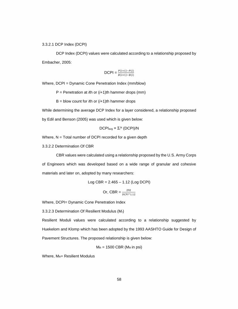
58

3.3.2.1 DCP Index (DCPI)

DCP Index (DCPI) values were calculated according to a relationship proposed by

Embacher, 2005:

DCPI = 𝑃(𝑖+1)−𝑃(𝑖)

𝐵(𝑖+1)−𝐵(𝑖)

Where, DCPI = Dynamic Cone Penetration Index (mm/blow)

P = Penetration at ith or (i+1)th hammer drops (mm)

B = blow count for ith or (i+1)th hammer drops

While determining the average DCP Index for a layer considered, a relationship proposed

by Edil and Benson (2005) was used which is given below:

DCPIavg = ΣiN (DCPI)/N

Where, N = Total number of DCPI recorded for a given depth

3.3.2.2 Determination Of CBR

CBR values were calculated using a relationship proposed by the U.S. Army Corps

of Engineers which was developed based on a wide range of granular and cohesive

materials and later on, adopted by many researchers:

Log CBR = 2.465 – 1.12 (Log DCPI)

Or, CBR = 292

𝐷𝐶𝑃𝐼^1.12

Where, DCPI= Dynamic Cone Penetration Index

3.3.2.3 Determination Of Resilient Modulus (Mr)

Resilient Moduli values were calculated according to a relationship suggested by

Huekelom and Klomp which has been adopted by the 1993 AASHTO Guide for Design of

Pavement Structures. The proposed relationship is given below:

MR = 1500 CBR (MR in psi)

Where, MR= Resilient Modulus

59

3.3.2.4 Determination of Unconfined Compressive Strength (Qu)

Values of unconfined compressive strength from DCP measurements were calculated

according to relationship proposed by Patel and Patel (2012) which was developed based

on CH, CL, SC and SM-SC soil to correlated DCP and UCS value.

UCS = 4.349 (DCPI)-1.09 (R2=0.968)

3.3.3 Geogauge Test

For each point considered for Geogauge, at least three measurements were taken and

then averaged to determine the stiffness of the pavement layer. Geogauge measurement

is sensitive to the seating procedure of the foot. Close contact with the surrounding layer

is necessary for the stiffness to be measured properly. Thus, to ensure close contact with

the immediate pavement layer, a wet sand layer (1

4"~

1

8") was placed on the pavement for

the point to be measured with Geogauge. The wet sand layer ensured the proper contact

between the Geogauge foot and the pavement layer. Some Geogauge test photos from

the field tests are shown below in Figure 3.2.

Figure 3.12: Geogauge Test Photos

60

3.3.4 Analysis Of Geogauge Data

3.3.4.1 Determination of Young’s Modulus, (E)

The value of stiffness, K (in MN/m) obtained from Geogauge has been converted

into Young’s Modulus (E) (in MPa) according to a relationship proposed by CAN Consulting

Engineers. The relationship is given below:

E= K∗(1−𝑣^2 )

1.77∗𝑅


E= Modulus of Elasticity (MPa)

𝑣 = Poisson’s Ratio (assumed as 0.35)


3.3.5 Nuclear Density Gauge Test

Nuclear Density Gauge test was performed with the help of Texas Department of

Transportation (TxDOT) officials at the site. Apart from operating the Gauge during

measurement, every kind of cooperation was provided to TxDOT officials to ensure the

proper measurement using Nuclear Density Gauge at site. Some of the test photos using

Nuclear Density Gauge are shown in Figure 3.13.

Figure 3.13: Nuclear Density Gauge Test Photos

61

3.3.6 Analysis Of Nuclear Density Gauge Test Data

The Nuclear Density Gauge test was performed with the help of TxDOT officials at site.

The density and moisture content data provided by the TxDOT officials were later used in

this study to compare with the Geogauge test data at site.

62

CHAPTER 4

RESULTS AND ANALYSIS

4.1 Introduction

Field assessment for the in-situ tests was performed on base materials for Horseshoe

Project. Analysis of the data obtained from the tests performed for the Horseshoe Project

will be discussed in this chapter.

4.2 Data Collection

For the Horseshoe project, Dynamic Cone Penetrometer (DCP) and Geogauge tests have

been performed on different test locations. Nuclear Density Gauge (NDG) test was also

performed to evaluate the in-situ moisture content and density of the compacted material

with the help of TxDOT officials.

4.3. Field Tests On Avery St. (Location-1)

4.3.1 Approximation Of Level Of Compaction From DCPI Profile With Depth

The DCP Index profiles obtained from the Dynamic Cone Penetrometer Tests performed

on 9 points across the width of the roadway are presented in Figure 4.1.

63

Figure 4.2: DCPI profile across depth of the pavement

DCPI values were observed within the range of 0-8 mm/blow for the upper 6” of cement

stabilized base layer for P2-P8 points. A higher initial value of DCPI can be observed for

each of the cases at the beginning of the penetration and this might happen due to the

presence of open graded layer at the top of the pavement. It is worth mentioning that a

heavy rainfall was observed before the test performed on June 9, 2014.

The values of DCPI vary from 3-22 mm/blow for the immediate 6” after the cement treated

base layer which constitutes of 4% lime treated subgrade, for the points P2-P8. An increase

in the values of DCPI from base layer to subgrade layer was observed which might have

taken place due to the decrease in resistance of the subgrade layer than the base layer.

The DCPI values vary within 8-47 mm/blow for the lower 12” (compacted subgrade) as

presented in the drawings.

The DCPI values obtained from P1 and P9 points do not follow the same range obtained

from P2-P8 points. It can be observed that for P1 and P9, the DCPI values vary within 4-

0

5

10

15

20

25

30

0 10 20 30 40 50 60 70D

ep

th (

inc

h)

DCP index (mm/blow)

P1

P2

P3

P4

P5

P6

P7

P8

P9

Corner Points (P1 and P9)

64

31 mm/blow for the upper 6” cement treated base layer, 11-60 mm/blow for 6” lime treated

subgrade and 24-52 mm/blow for the lower 12” of compacted subgrade, respectively. DCPI

profiles of P1 and P9 do not follow the range obtained from other points (P2-P8). P1 and

P9 points were considered at the edge of the roadway which might indicate that the level

of compaction along the edge of the roadway were not the same for all the three layers

(cement treated base layer, lime treated subgrade layer, compacted subgrade layer) if

compared to the compaction level obtained from the other points (P2-P8). There is a

possibility that the level of confinement at the edge of the pavement might have affected

the DCP penetration rate at the edge of the pavement.

4.3.2 Determination Of Layer Thickness From DCPI Profile

DCPI values obtained from a single point (here, P6) show that the values change

significantly due to the change in the material properties for different layers which is

presented below in Figure 4.2.

DCPI profile obtained from P6 that the DCPI values change gradually from layer to layer.

Cement treated base layer provides lowest DCPI values and the compacted subgrade

layer giving the highest DCPI values respectively. From the Figure 4.2, it can be seen that

for the cement treated base layer, the DCPI values change from 1 mm/blow to 5 mm/blow

providing a thickness of 6 inch for the cement treated base layer, whereas, for the lime

treated subgrade layer, the DCPI values change from 4 mm/blow to 13 mm/blow which

indicates a 6” thick lime treated subgrade layer following the base layer on the top.

Afterwards, the DCPI increases with increasing depth and finally reaches a value of 40

mm/blow in the compacted subgrade layer. Based on the DCPI profile across depth of the

pavement obtained from P6, three layers can easily be differentiated which indicates the

effectiveness of using Dynamic Cone Penetrometer as an in-situ pavement testing

equipment during construction.

65

Figure 4.3: DCPI profile across depth of the pavement obtained from P6

Later the depth of each layer obtained from DCP Index profiles obtained from each points

the tests have been performed was verified from the design thickness which can be seen

from Figure 4.2. It can be seen that the depth of each layer distinguished from DCP Index

profiles was observed within 0.5 inch from the design value. A linear trend of DCP Index

values for each layer also provides a specific DCP Index value for a certain layer from

which any effect of presence of hard layer or rock can be eliminated while calculating the

material properties of a certain layer. Comparison of resilient moduli values obtained from

the slope of the DCP Index profile and the average resilient moduli value obtained from

each 1 inch segment of the pavement will be shown later in this chapter.

0

5

10

15

20

25

0 10 20 30 40 50D

ep

th (

inc

h)

DCP index (mm/blow)

P6

Layer 1

Layer 2

Layer 3

6" Cement Stablized Base with

6" Lime Treated Subgrade

Compacted Subgrade

66

4.3.3 Resilient Moduli Profile Along Depth

The values of Resilient Moduli can be plotted with depth to see the variation of resilient

moduli values across the depth of the pavement as the material properties changes across

depth. It can be observed that for P2-P8, the resilient moduli values changes within a range

of 40,744-713,948 psi for the upper 6” of cement treated base layer which is presented in

Figure 4.3. Upper 6” cement treated base layer provided the highest resistance to the

penetrating cone which results in higher range of resilient moduli values across this layer.

For the immediate 6” lime treated subgrade layer, resilient moduli vary within a range of

17,749-138,218 psi for P2-P8. For compacted subgrade, Mr values vary from 5,869-40,744

psi.

Figure 4.4: Resilient Moduli Profile across depth of the pavement

The upper 6” of cement treated base layer provides the highest support leading to a higher

range of resilient moduli values for the upper layer. For the points considered both at the

edge of the roadway, resilient moduli profiles are not same when compared to the other

0

5

10

15

20

25

30

1000 10000 100000 1000000

De

pth

(in

ch

)

Resilient Modulus, Mr (psi)

P1P2P3P4P5P6P7P8P9

Corner Points (P1 and P9)

6" Cement Stabilized Base

6" Lime Stablized Subgrade

Compacted Subgrade

67

points (P2-P8). For these two points (P1 and P9), the resilient moduli values were within a

range of 9,355-127,940 psi for the upper 6” of cement treated base layer, 4,465-28,873 psi

for the immediate 6” of lime treated subgrade layer and 7,673-18,958 psi for 12” of

compacted subgrade as presented in Figure 4.3.

4.3.4 Variation Of Resilient Moduli In Different Layers

The resilient modulus was determined at each DCPI value. The predicted Mr value along

the layer was averaged to determine the Mr at each point of the layer. The average resilient

moduli values along each layer is presented in Figure 4.4.

Figure 4.5: Variation of Resilient Moduli in Different Layers

Resilient moduli values in the upper 6” cement stabilized base layers vary from 40,500-

374,078 psi. The resilient moduli vary from 7,513-73,351 psi for 6” lime treated subgrade

layer and in the compacted subgrade layers, resilient moduli values were within a range

8,458-20,266 psi. For each of the three layers, the lowest value for each respective layer

1000

10000

100000

1000000

Re

sil

ien

t M

od

ulu

s,

Mr

(p

si)

Point ID

Cement Stabilized Base with Prime Coat (6")Lime Treated Subgrade (6"~12")Compacted Subgrade (12"~18")Compacted Subgrade (18"~24")

P1 P2 P3 P4 P5 P6 P7 P8 P9

P1

P2

P3

P4

P5

P6

P7

P8

P9

68

is found at the edge of the roadway which might have occurred due to the lack of

confinement at the edge of the pavement.

4.3.5 Variation Of Unconfined Compressive Strenth In Base Layer Across Width Of The

Pavement

Figure 4.5 shows the variation of unconfined compressive strength (UCS) of the points

considered in the topmost 6” cement stabilized base layer across the width of the

pavement. The lowest UCS was found at both edges of the pavement (P1 and P9). The

UCS value at the edge of the pavement varied between 73.7 psi – 76.4 psi whereas, for

the other points (P2-P8), UCS was observed within a range of 269.4 psi – 619.2 psi. The

UCS value across the width of the pavement was calculated according to a relationship

proposed by Patel and Patel (2012).

Figure 4.6: Variation of Unconfined Compressive Strength in base layer across width of pavement at Location-1

0

100

200

300

400

500

600

700

P1 P2 P3 P4 P5 P6 P7 P8 P9

Un

con

fin

ed C

om

pre

ssiv

e S

tren

gth

, q

u (

psi

)

P1 P2

P3

P4

P5

P6

P7

P8

P9

69

The UCS value across the width of the pavement was calculated according to a relationship

proposed by Patel and Patel (2012).

4.3.6 Variation Of Young’s Moduli From Geogauge

For the location on Avery St near Tom Landry Fwy (I-30), Dallas, TX, nine points at 5’ apart

were considered to be measured with Geogauge. Proper contact was ensured before each

measurement with the placement of wet sand layer between the Geogauge foot and the

pavement layer. Young’s moduli values measured with Geogauge will be considered as

the property of the top layer of the pavement (cement stabilized base with prime coat). It

can be seen from the graph presented in Figure 4.6 that the lowest Young’s Modulus value

(28,900 psi) was found at the corner point (P9) of the pavement section. Young’s Moduli

value varied from 42,337 psi to 66,696 psi for P1-P8 points. The highest moduli value was

obtained at P5 (66,696 psi) which was at the middle of the pavement.

Figure 4.7: Variation of Young’s Modulus across Pavement

0

10000

20000

30000

40000

50000

60000

70000

80000

Yo

un

g's

Mo

du

lus

(p

si)

Point ID

Young's Modulus (Geogauge)

P1 P2 P3 P4 P5 P6 P7 P8 P9

P1P2P3P4P5P6P7P8P9

Excellent

Good

Weak

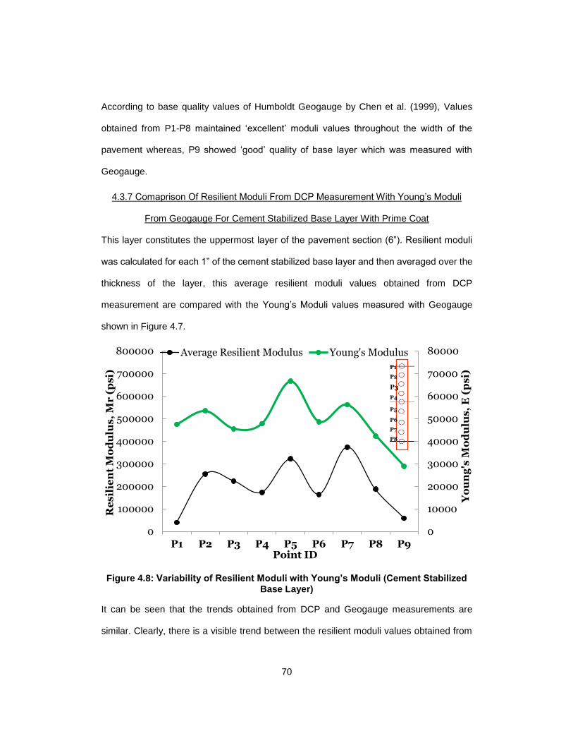
70

According to base quality values of Humboldt Geogauge by Chen et al. (1999), Values

obtained from P1-P8 maintained ‘excellent’ moduli values throughout the width of the

pavement whereas, P9 showed ‘good’ quality of base layer which was measured with

Geogauge.


From Geogauge For Cement Stabilized Base Layer With Prime Coat

This layer constitutes the uppermost layer of the pavement section (6”). Resilient moduli

was calculated for each 1” of the cement stabilized base layer and then averaged over the

thickness of the layer, this average resilient moduli values obtained from DCP

measurement are compared with the Young’s Moduli values measured with Geogauge

shown in Figure 4.7.

Figure 4.8: Variability of Resilient Moduli with Young’s Moduli (Cement Stabilized Base Layer)

It can be seen that the trends obtained from DCP and Geogauge measurements are

similar. Clearly, there is a visible trend between the resilient moduli values obtained from

0

10000

20000

30000

40000

50000

60000

70000

80000

0

100000

200000

300000

400000

500000

600000

700000

800000

P1 P2 P3 P4 P5 P6 P7 P8 P9

Yo

un

g's

Mo

du

lus

, E

(p

si)

Re

sil

ien

t M

od

ulu

s,

Mr

(p

si)

Point ID

Average Resilient Modulus Young's Modulus

P1

P2

P3

P4

P5

P6

P7

P8

71

DCP measurements and the Young’s Moduli values measured with Geogauge. Although

there is a possibility of the increase in resilient moduli value if DCP rod penetrates through

a crushed concrete aggregate while obtaining the average material properties of a certain

layer, Geogauge can clearly capture this effect into its measurement which can be

observed from the similar trend provided by both DCP and Geogauge.

4.4 Field Tests Near I-35E Northbouth Frontage Road (Location-2)

4.4.1 Variation Of Young’s Moduli With Moisture Content

Eight points at 5’ apart from each other across the roadway were considered to measure

the variation of moduli values with Geogauge, Nuclear Density Gauge tests were also

performed at these points to see the variation of moisture content, dry density and wet

density with the change in moduli values. It has been observed that the moduli values

measured with Geogauge are affected with the slight change in moisture content which is

presented below in Figure 4.8.

Figure 4.9: Variation of Young’s Moduli with change in Moisture Content

0

2

4

6

8

10

12

14

0

10000

20000

30000

40000

50000

60000

70000

Mo

istu

re

Co

nte

nt

(%)

Yo

un

g's

Mo

du

lus

(p

si)

Point ID

Young's Modulus (Geogauge) Moisture content

P1 P2 P3 P4 P5 P6 P7 P8

P1

P2

P3

P4

P5

P6

P7

P8

Excellent

Good

Weak

72

The moduli values seem to increase with the increase in moisture content in the materials.

At all the points which were considered for the Geogauge and Nuclear Density Gauge

(NDG) tests to be performed, it was observed that the moduli values increase in all cases

as the moisture content increases. P1 and P8 were considered at the edge of the pavement

for the measurements to be taken, both were supposed to show the like-wise moduli values

because of level of compaction at both points. P1 was not totally located at the edge of the

roadway but rather more compacted areas were left apart from the width of the road which

was considered for the measurements. According to the base characterization values

provided by Chen et al., (1999), P1-P7 showed ‘excellent’ base quality while P8 which is

located at the edge of the pavement was of ‘good’ quality.

4.4.2 Variation Of Young’s Moduli With Change In Density

Change in Young’s Moduli values can be compared with the change in wet density

measured with Nuclear Density Gauge which is presented in Figure 4.9.

Figure 4.10: Variation of Young’s Moduli with change in Wet Density

100

105

110

115

120

125

130

135

140

0

10000

20000

30000

40000

50000

60000

70000

We

t D

en

sit

y, γ

m(p

cf)

Yo

un

g's

Mo

du

lus

(p

si)

Point ID


Wet Density (Nuclear Density Gauge)

P1 P2 P3 P4 P5 P6 P7 P8

P1

P2

P3

P4

P5

P6

P7

P8

73

The Young’s Moduli values increase with the increase in wet density. At P5, a sudden

decrease in moduli value can be observed with a sudden drop of wet density. This might

happen due to the non-uniformity of the compaction procedure during the placing of the

cement treated base layer or lime treated subgrade. As Geogauge takes 12 inch into

account while measuring the stiffness or moduli of the layer beneath, the non-uniformity of

compaction during the placing of material within the upper 12” depth might lead to a

decreased moduli value.

The same trend can also be found when moduli values measured at different points are

plotted with the change in dry density measured with the Nuclear Density Gauge (NDG)

which is presented below in Figure 4.10.

Figure 4.11: Variation of Young’s Moduli with change in Dry Density

100

105

110

115

120

125

0

10000

20000

30000

40000

50000

60000

70000

Dr

y D

en

sit

y, γ

d (

pc

f)

Yo

un

g's

Mo

du

lus

, E

(p

si)

Point ID

Geogauge ModulusDry Density (Nuclear Density Gauge)

P1 P2 P3 P4 P5 P6 P7 P8

P1

P2

P3

P4

P5

P6

P7

P8

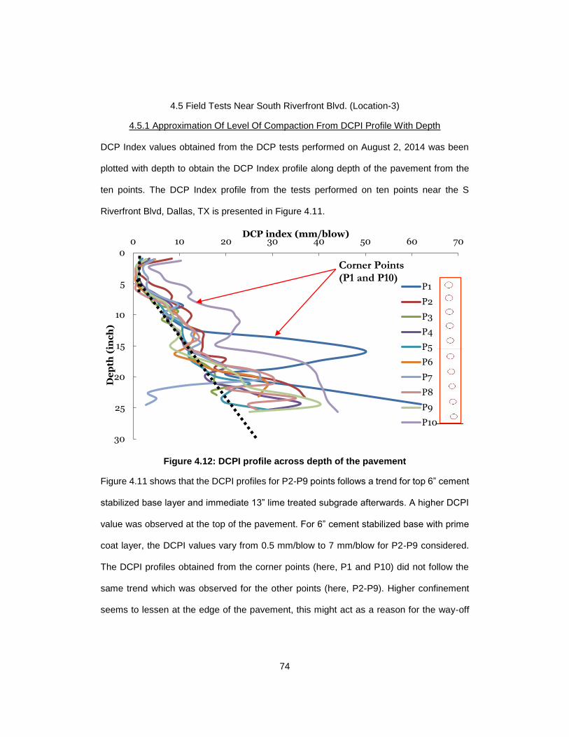
74

4.5 Field Tests Near South Riverfront Blvd. (Location-3)


DCP Index values obtained from the DCP tests performed on August 2, 2014 was been

plotted with depth to obtain the DCP Index profile along depth of the pavement from the

ten points. The DCP Index profile from the tests performed on ten points near the S

Riverfront Blvd, Dallas, TX is presented in Figure 4.11.


Figure 4.11 shows that the DCPI profiles for P2-P9 points follows a trend for top 6” cement

stabilized base layer and immediate 13” lime treated subgrade afterwards. A higher DCPI

value was observed at the top of the pavement. For 6” cement stabilized base with prime

coat layer, the DCPI values vary from 0.5 mm/blow to 7 mm/blow for P2-P9 considered.

The DCPI profiles obtained from the corner points (here, P1 and P10) did not follow the

same trend which was observed for the other points (here, P2-P9). Higher confinement

seems to lessen at the edge of the pavement, this might act as a reason for the way-off

0

5

10

15

20

25

30

0 10 20 30 40 50 60 70

De

pth

(in

ch

)

DCP index (mm/blow)

P1

P2

P3

P4

P5

P6

P7

P8

P9

P10

Corner Points(P1 and P10)

75

trend than the DCPI profiles obtained from P2-P9. For the 13” lime treated subgrade layer,

the DCPI varied from 3.3 mm/blow to 25 mm/blow for the points from P2 to P9 considered.


Different trend of DCPI values for different materials will facilitate the use of DCPI profile

along depth to distinguish layers of the pavement section. Considering the DCPI profile

obtained from P2, different layers of the pavement section can easily be distinguished from

the trend that has been observed for separate layers of the pavement. DCPI profile along

depth for point P2 has been presented below in the Figure 4.12.


From the DCPI profile obtained from P2 point, it can clearly be seen that the DCPI value

change gradually from one layer to another. For instance, DCPI value was observed within

0.69 mm/blow - 7 mm/blow for the top 6” cement stabilized base layer. Afterwards, it started

increasing gradually for the immediate 13” lime treated subgrade of the pavement section.

The higher DCPI value for the first inch of the pavement was ignored while determining the

0

5

10

15

20

25

0 10 20 30 40

De

pth

(in

ch

)

DCP index (mm/blow)

P2

Layer 1

Layer 2

Layer 3

6" Cement Stablized Base with Prime Coat


Compacted Subgrade

76

layer thickness because there might be a possibility that higher initial DCPI value may

result due to positioning of the DCPI rod at the beginning of the pavement or the climatic

effect on the top of the pavement. For the next 13” lime treated subgrade, the DCPI value

varied from 8.3 mm/blow to 20 mm/blow and for the next part of the pavement which is

compacted subgrade, the DCPI values started increasing gradually afterwards.

The determination of different layers using DCPI profiles along the depth of the pavement

was later verified with the design thickness of the pavement section. It has been found that

the layer thickness obtained from the DCPI profiles varied within a range of 0.5 inch when

compared with the design thickness.


The resilient moduli value obtained for different DCPI values for each 1” of the pavement

was plotted with the depth to see the change of moduli values across the depth of the

pavement which is presented in Figure 4.13.


0

5

10

15

20

25

30

1000 10000 100000 1000000

De

pth

(in

ch

)


P2

P3

P4

P5

P6

P8

P9

6" Cement Stablized

Base with Prime Coat


Compacted Subgrade

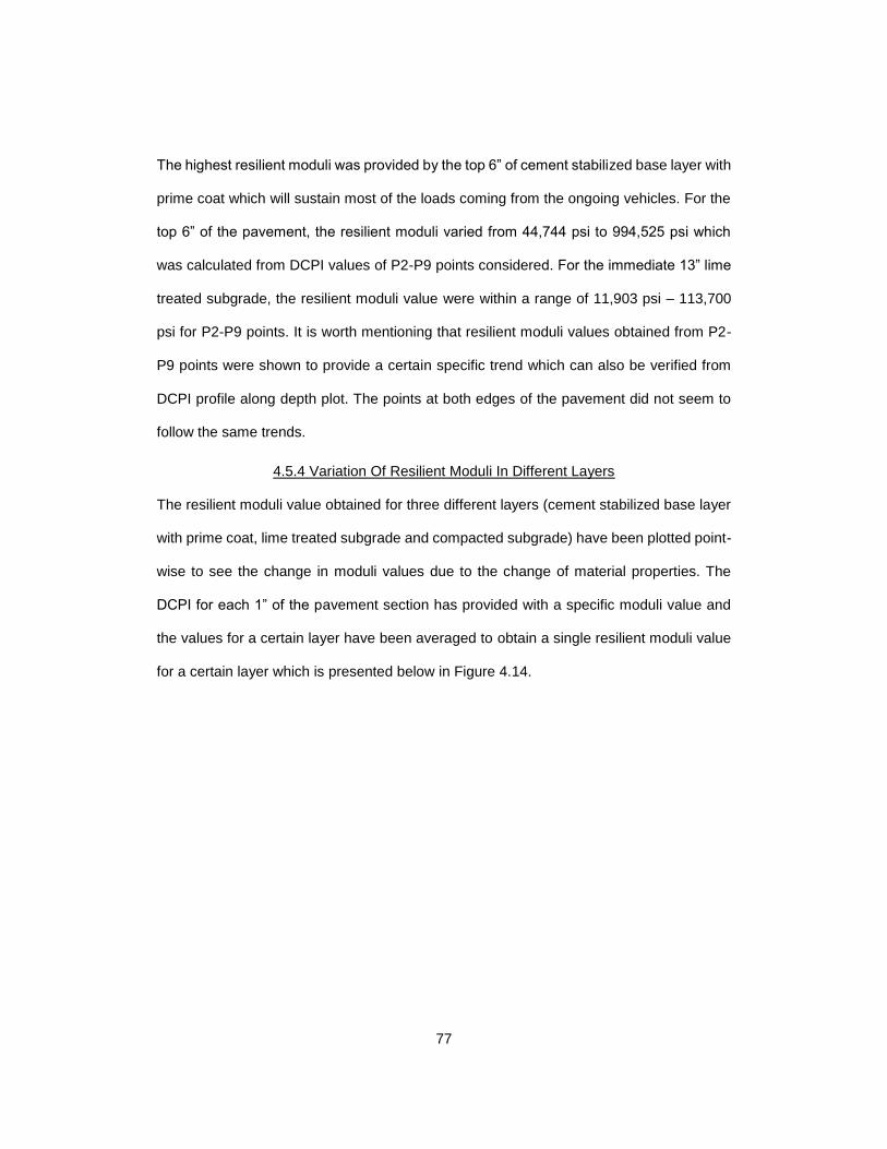
77

The highest resilient moduli was provided by the top 6” of cement stabilized base layer with

prime coat which will sustain most of the loads coming from the ongoing vehicles. For the

top 6” of the pavement, the resilient moduli varied from 44,744 psi to 994,525 psi which

was calculated from DCPI values of P2-P9 points considered. For the immediate 13” lime

treated subgrade, the resilient moduli value were within a range of 11,903 psi – 113,700

psi for P2-P9 points. It is worth mentioning that resilient moduli values obtained from P2-

P9 points were shown to provide a certain specific trend which can also be verified from

DCPI profile along depth plot. The points at both edges of the pavement did not seem to

follow the same trends.


The resilient moduli value obtained for three different layers (cement stabilized base layer

with prime coat, lime treated subgrade and compacted subgrade) have been plotted point-

wise to see the change in moduli values due to the change of material properties. The

DCPI for each 1” of the pavement section has provided with a specific moduli value and

the values for a certain layer have been averaged to obtain a single resilient moduli value

for a certain layer which is presented below in Figure 4.14.

78


It can be seen that the resilient moduli values for the topmost 6” cement stabilized base

layer with prime coat varied from 131,423 psi to 623,285 psi, 14,556 psi – 41,950 psi for

immediate 13” lime treated subgrade beneath the base layer. From the resilient moduli

profile, it is clearly visible that there might be possible anomaly in the compacted subgrade.

There might be a possibility that a hard layer may exist in the compacted subgrade which

might lead to lesser DCPI value and thus higher resilient moduli value at that certain point

(P7). Detection of possible hard layer in the middle of the pavement can also be understood

from the variability plot of resilient moduli value for the points considered which will be

shown later.


Pavement

Figure 4.15 shows the variation of UCS in the base layer of the ten points considered for

the DCP tests to be performed across the width of the pavement. The lowest UCS value

1000

10000

100000

1000000R

es

ilie

nt

Mo

du

lus

, M

r (

ps

i)

Point ID

Cement Stabilized Base Layer (6")

Lime Treated Subgrade (6"~19")

Compacted Subgrade (19"~25")

P1 P2 P3 P4 P5 P6 P7 P8 P9 P10

P1

P2

P3

P4

P5

P6

P7

P8

P9

P10

Possible Anomaly

79

(81.9 psi) was found at P10 which is located at the edge of the pavement. From P1 to P9,

the UCS value varied from 210 psi – 1023.5 psi where the highest UCS value was found

at P8.


4.5.6 Variation Of Young’s Moduli From Geogauge

Ten points at 7 ft apart were considered near the S Riverfront Blvd., Dallas, TX near I-35E

for the field tests on August 2, 2014. First test performed on a single point was Geogauge

test because it takes measurement without disturbing the pavement layer. A wet sand layer

was placed before placing the Geogauge foot onto the soil to ensure the proper contact

between the Geogauge foot and the pavement material. At lease, three close

measurements were taken to avoid any error in taking measurements and then averaged

to evaluate material properties for a certain test point considered. The variation of Young’s

moduli (E) across the width of the pavement can be seen from the Figure 4.16. For the top

base layer of the pavement, the Young’s modulus for the layer considered varied from

26,384 psi to 76,320 psi. The highest value was found at P8 with the use of Geogauge

0

200

400

600

800

1000

1200

P1 P2 P3 P4 P5 P6 P7 P8 P9 P10

Un

co

nfi

ne

d C

om

pr

es

siv

e

Str

en

gth

, q

u (

ps

i)

P1 P2

P3

P4

P5

P6

P7

P8

P9

P10

80

which also satisfies the moduli value obtained with the use of Dynamic Cone Penetrometer

which can be seen from Figure 4.16.


From the values presented in Figure 4.16, All the points (P1-P10), except P6 and P10,

showed ‘excellent’ base quality whereas P6 and P10 provided ‘good’ base quality

according to the base quality characterization values provided by Chen et al., (1999).



For the 6” cement stabilized base layer with prime coat, variability of resilient moduli values

were plotted for all the points considered which is shown in Figure 4.17.

0

10000

20000

30000

40000

50000

60000

70000

80000

Yo

un

g's

Mo

du

lus

, E

(p

si)

Point ID


P1 P2 P3 P4 P5 P6 P7 P8 P9 P10

P1 P2

P3

P4 P5 P6

P7 P8 P9 P10 Excellent

Good

Weak

81


From the Young’s moduli values across the points (P1-P10) measured with Geogauge that

the Geogauge is able to capture the effect of presence of any crushed concrete aggregate

in the layer where resilient moduli value measured with DCP is higher and thus showing a

similar trend like a trend which was observed in values of Young’s moduli measured with

Geogauge.

4.6 Field Tests Near Jefferson Viaduct Blvd. (Location-4)

4.6.1 Variation Of Young’s Moduli With Moisture Content

Six points were considered for NDG and Geogauge tests to be performed near the

Jefferson Viaduct Blvd., Dallas, TX Variation in Young’s moduli (E) was plotted with the

change in moisture content measured with Nuclear Density Gauge as presented in Figure

4.18. Three close measurements were averaged to obtain a single modulus value for a

single point considered. It has been observed that the Young’s moduli value measured with

Geogauge varied from 8,447 psi to 57,737 psi. The lowest modulus was found at one edge

0

10000

20000

30000

40000

50000

60000

70000

80000

0

100000

200000

300000

400000

500000

600000

700000

800000

P1 P2 P3 P4 P5 P6 P7 P8 P9 P10

Yo

un

g's

Mo

du

lus

, E

(p

si)

Re

sil

ien

t M

od

ulu

s,

Mr

(p

si)

Point ID

P1 P2

P3

P4 P5 P6

P7 P8 P9 P10

82

of the pavement (P6). The moisture content (w) measured with Nuclear Density Gauge

varied from 11.2% to 14.6% for P1-P6. All the properties measured with NDG was at the

depth 6 inch from the top of the pavement which represents cement stabilized base layer

with prime coat.

Figure 4.19: Variation of Young’s Moduli with change in Moisture Content

It can be observed that the point ID- P1, P4 and P5 showed ‘excellent’ base quality

whereas, P2 and P3 showed ‘good’ base quality. On the other hand, P6 which is located

at the edge of the pavement, provided ‘weak’ base layer support according to the

characterization value provided by Chen et al., (1999).

4.6.2 Variation Of Young’s Moduli With Change In Density

The change in Young’s moduli measured with Geogauge with the change in wet density

measured with Nuclear Density Gauge is shown in Figure 4.19 below. It is evident that with

the increase in wet density, Young’s moduli values increase across the points considered

0

2

4

6

8

10

12

14

16

0

10000

20000

30000

40000

50000

60000

Mo

istu

re

Co

nte

nt,

w (

%)

Yo

un

g's

Mo

du

lus

, E

(p

si)

Point ID

Young's Modulus (Geogauge)Moisture content

P1 P2 P3 P4 P5 P6

P1

P2

P3

P4

P5

P6

Excellent

Good

Weak

83

along the width of the pavement. The wet density varied from 109.6 pcf to 125.9 pcf. The

lowest wet density was found at the edge of the pavement (P6).

Figure 4.20: Variation of Young’s Moduli with change in Wet Density

The same trend was also observed when dry density across the points was plotted against

the Young’s moduli value measured with Geogauge as presented in Figure 4.20. As the

Dry density increases, Young’s moduli values increase and the vice versa. The dry density

of the points considered was observed within a range of 97.5 pcf – 111.2 pcf.

80

85

90

95

100

105

110

115

120

125

130

0

10000

20000

30000

40000

50000

60000

We

t D

en

sit

y, γ

m(p

cf)

Yo

un

g's

Mo

du

lus

, E

(p

si)

Point ID

Young's Modulus (Geogauge)Wet Density (Nuclear Density Gauge)

P1 P2 P3 P4 P5 P6

P1

P2

P3

P4

P5

P6

84

Figure 4.21: Variation of Young’s Moduli with change in Dry Density

4.7 Field Tests Near Sylvan Ave. (Location-5)


DCP Index values obtained for 1” penetration into the pavement layer by the DCP rod is

plotted against the depth to obtain the DCPI profile along depth which is presented below

50

60

70

80

90

100

110

120

0

10000

20000

30000

40000

50000

60000

Dr

y D

en

sit

y, γ

d (

pc

f)

Yo

un

g's

Mo

du

lus

, E

(p

si)

Point ID

Young's Modulus (Geogauge)Dry Density (Nuclear Density Gauge)

P1 P2 P3 P4 P5 P6

P1

P2

P3

P4

P5

P6

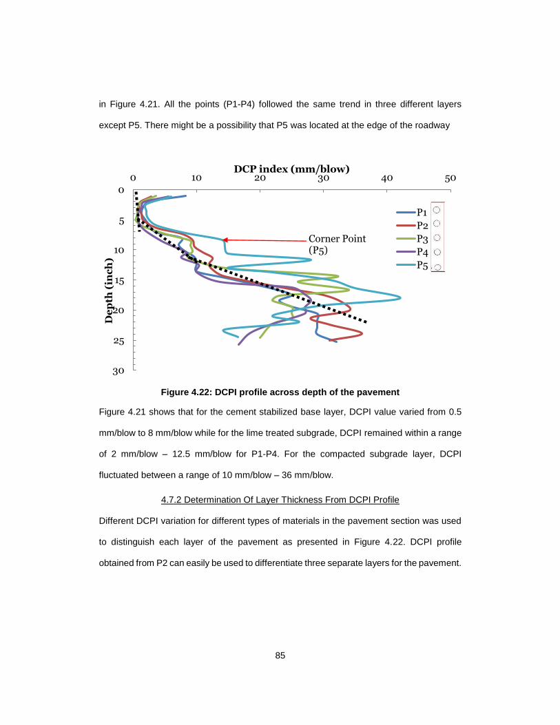
85

in Figure 4.21. All the points (P1-P4) followed the same trend in three different layers

except P5. There might be a possibility that P5 was located at the edge of the roadway


Figure 4.21 shows that for the cement stabilized base layer, DCPI value varied from 0.5

mm/blow to 8 mm/blow while for the lime treated subgrade, DCPI remained within a range

of 2 mm/blow – 12.5 mm/blow for P1-P4. For the compacted subgrade layer, DCPI

fluctuated between a range of 10 mm/blow – 36 mm/blow.


Different DCPI variation for different types of materials in the pavement section was used

to distinguish each layer of the pavement as presented in Figure 4.22. DCPI profile

obtained from P2 can easily be used to differentiate three separate layers for the pavement.

0

5

10

15

20

25

30

0 10 20 30 40 50

De

pth

(in

ch

)

DCP index (mm/blow)

P1

P2

P3

P4

P5

Corner Point (P5)

86


Figure 4.22 shows that DCPI change within 1.3 mm/blow – 8.3 mm/blow for the top 6”

cement stabilized base layer and varied between 3.6 mm/blow – 10 mm/blow for the

immediate 6” lime treated subgrade and between 10 mm/blow – 32 mm/blow for the rest

of the compacted subgrade. Higher initial DCPI was ignore while establishing the thickness

of the top layer in this case. Later, these determined thicknesses of the layers were verified

with the design thickness to evaluate the efficiency of Dynamic Cone Penetrometer as an

in-situ pavement evaluation equipment. The determined thicknesses was within 0.5 inch

when compared with the design thickness.


The resilient moduli values calculated from the DCPI obtained from each 1” depth of the

pavement section are plotted against the depth to obtain the resilient moduli profile along

depth which is presented in Figure 4.23.

0

5

10

15

20

25

30

0 10 20 30 40D

ep

th (

inc

h)

DCP index (mm/blow)

P1

Layer 1

Layer 2

Layer 3

6" Cement Stabilized Base with Prime Coat


Compacted Subgrade

87

Figure 4.24: Resilient Moduli Profile across depth of the pavement

The top 6” cement stabilized base layer provided the highest resilient moduli values among

the three layers encountered. The resilient moduli varied within a range of 40,745 psi –

573,704 psi for the topmost 6” cement stabilized base layer for P1-P4 considered whereas,

for the immediate 6” lime treated subgrade, variation was within 25,873 psi – 201,480 psi.

Resilient moduli values varied from 7,913 psi – 33,220 psi in the compacted subgrade layer

for P1-P4 points.


Three different layers (cement stabilized base with prime coat, lime treated subgrade and

compacted subgrade) provided three ranges of resilient moduli values which can be seen

layer-wise from Figure 4.24. For cement stabilized base layer, resilient moduli varied from

190,345 psi to 502,206 psi while for lime treated subgrade, it varied from 32,990 psi to

76,660 psi. Resilient moduli values were observed within a range of 12,422 psi – 16,094

psi for compacted subgrade layer.

0

5

10

15

20

25

30

1000 10000 100000 1000000D

ep

th (

inc

h)


P1

P2

P3

P4

P5

Corner Point (P5)

6" Cement Stablized Base with Prime Coat


Compacted Subgrade

88



Pavement

Figure 4.25 presents the variation of unconfined compressive strength (UCS) in the top 6”

cement stabilized base layer across the width of the pavement section. From P1-P5

considered, the UCS value varied from 238.2 psi – 829 psi where the lowest value was

found at P5 and the highest value of UCS was found at P3 which was located in the middle

of the width of the pavement.

1000

10000

100000

1000000R

es

ilie

nt

Mo

du

lus

, M

r (

ps

i)

Point ID

Cement Stabilized Base Layer (6")

Lime Treated Subgrade (6")

Compacted Subgrade (12"~24")

P1 P2 P3 P4 P5

89


4.7.6 Variation Of Young’s Moduli From Geogauge:

Wet sand layer was placed on the ground before taking measurement with Geogauge on

five points set at 4 ft apart. Three close measurements were taken at each point considered

to eliminate any scope of errors while measuring with Geogauge because proper contact

between Geogauge foot and pavement layers is needed to ensure good measurement.

The variation in Young’s moduli across the five points is presented in Figure 4.26. From

P1-P5, Young’s moduli measured with Geogauge varied from 60,490 psi to 75,410 psi for

the tests performed on October 3, 2014.

0

100

200

300

400

500

600

700

800

900

P1 P2 P3 P4 P5

Un

co

nfi

ne

d C

om

pr

es

siv

e S

tre

ng

th,

qu

(p

si)

Point ID

90


All the points (P1-P5) provided ‘excellent’ base layer support according to the values

characterization values provided by Chen et al., (1999) which can be seen from Figure

above.



Within P1-P5 considered, P3 showed highest variability in resilient moduli values within a

range of 140,629 psi – 502,493 psi. Overall, Young’s moduli values measured with

Geogauge showed similar trend with the resilient moduli measured with Dynamic Cone

Penetrometer which is shown below in Figure 4.27. Geogauge takes 9”~12” into account

while taking it measurement, it is evident from the trend that the 6” cement stabilized base

layer seems to have the major effect on the values measured with Geogauge because of

its similarity with resilient moduli trend measure with DCP.

0

10000

20000

30000

40000

50000

60000

70000

80000Y

ou

ng

's M

od

ulu

s (

ps

i)

Point ID


P1 P2 P3 P4 P5

Excellent

Good

Weak

91


4.8 Comparison With Literature

4.8.1 Comparison Of Resilient Modulus From DCPI

4.8.1.1 Cement Stabilized Base With Prime Coat

Gaspard (2000) evaluated the resilient moduli values of cement stabilized base material

for different cement content. The average resilient moduli value determined by Gaspard

based on extensive field test performed for cement stabilized base materials for 7%, 8%,

9% and 10% cement content were 174,000 psi, 229,000 psi, 237,000 psi and 145,000 psi,

respectively. While in Texan condition, laboratory test conducted on stabilized 4.5% and

3% cement treated base materials by Guthrie et al. (2001) generated a mean resilient

moduli value of 381,170 psi and 276,722 psi, respectively. To compare resilient moduli

value to other values mentioned in literature, resilient moduli values from every point

considered for a location are averaged to obtain a specific moduli value for a certain

location for 6” cement stabilized base layer with prime coat which is presented in Figure

0

10000

20000

30000

40000

50000

60000

70000

80000

0

100000

200000

300000

400000

500000

600000

700000

800000

P1 P2 P3 P4 P5

Yo

un

g's

Mo

du

s,

E (

ps

i)

Re

sil

ien

t M

od

ulu

s,

Mr

(p

si)

Point ID

Average Resilient ModulusYoung's Modulus (Geogauge)

92

4.28. Three locations (Avery St, S Riverfront Blvd. and Sylvan Ave.) where the DCP tests

performed provided three specific resilient moduli value for the top cement stabilized base

layer. The location-wise resilient moduli values and values determined by Gaspard (2000)

and Guthrie et al. (2001) are given in the Table 4.1 below.

Table 4.1: Location-wise Resilient Moduli values with Literature Moduli Values (Cement Stabilized Base Layer)

Location

Resilient

Modulus,

Mr (psi)

Material Type Test Type

Location-1 (Avery St.) 200,030

Cement Stabilized Base Materials

Field Test

Location-3 (S Riverfront Blvd.) 302,110 Cement Stabilized Base Materials

Field Test

Location-5 (Sylvan Ave.) 292,407 Cement Stabilized Base Materials

Field Test

7% Stabilized CTB (Gaspard, 2000) 174,000 Cement Stabilized Base Materials

Field Test


Field Test


Field Test

10% Stabilized CTB (Gaspard, 2000)

145,000 Cement Stabilized Base Materials

Field Test

3% Stabilized CTB (Guthrie et al., 2001)


Laboratory Test

4.5% Stabilized CTB (Guthrie et al., 2001)


Laboratory Test

93

Figure 4.29: Comparison between Resilient Moduli values obtained from Field Tests and Literature (Cement Stabilized Base Layer)

4.8.1.2 Lime Stabilized Subgrade

Sargand (2000) conducted Dynamic Cone Penetrometer Test on lime treated Livingston

soil in Ohio to determine the limiting DCPI value for subgrade acceptance and he

concluded that the limiting DCPI for lime treated Livingston subgrade soil is 5.23 mm/blow.

This DCPI value is converted into resilient modulus and thus compared to the average

moduli value obtained by averaging the value from each successive 1” depth of the lime

treated subgrade which is presented in Figure 4.29. Table 4.2 shows the resilient moduli

values obtained from field tests performed at Avery St, S Riverfront Blvd. and Sylvan Ave.,

respectively.

0

50000

100000

150000

200000

250000

300000

350000

400000

450000

Avery St.(4.5%)

SRiverfront

Blvd.(4.5%)

SylvanAve.

(4.5%)

7%Stabilized

CTB(Gaspard,

2000)

8%Stabilized

CTB(Gaspard,

2000)

9%Stabilized

CTB(Gaspard,

2000)

10%Stabilized

CTB(Gaspard,

2000)

3%stabilized

CTB(Guthrie

et al.,2001)

4.5%Stabilized

CTB(Guthrie

et al.,2001)

Re

sil

ien

t M

od

ulu

s,

Mr

(p

si)

94

Table 4.2: Location-wise Resilient Moduli values with Literature Moduli Values (Lime Treated Subgrade Layer)

Location

Resilient

Modulus,

Mr (psi)

Test Type Material

Type

Location-1 (Avery St.) 46,229 Field Test Plastic Clay

Location-3 (S Riverfront Blvd.) 32,813 Field Test Plastic Clay

Location-5 (Sylvan Ave.) 45,509 Field Test Plastic Clay

Livingston Lime Treated Soil (Sargand, 2000) 68,668 Field Test –

Lime Stabilized Texas soil (Little et al., 1995) 70,000 Laboratory

Test Plastic Clay

Figure 4.30: Comparison between Resilient Moduli values obtained from Field Tests and Literature (Lime treated Subgrade Layer)

0

10000

20000

30000

40000

50000

60000

70000

80000

Avery St. S RiverfrontBlvd.

Sylvan Ave. Livingston Soil(Sargand, 2000)

TX LimeStabilized Soil(Little et al.,

1995)

Re

sil

ien

t M

od

ulu

s,

Mr

(p

si)

95

From Figure 4.29, it can be seen that the resilient moduli values obtained for lime-treated

subgrade layer varied at Location-1 varied 32.7% from the moduli value obtained from the

test performed on Livingston soil, resilient moduli obtained from Location-3 varied 52.2%

and moduli value from Location-5 varied 33.7%, respectively. According to Little et al.,

(1995), resilient moduli of lime stabilized subgrade soil can reach up to 70,000 psi.

4.8.1.3 Compacted Subgrade

Sargand (2000) performed resilient modulus test on the soil sample collected for US30 and

DEL23 projects in Ohio. The resilient moduli values obtained from different tests performed

by Sargand are presented below in Table 4.3 with the average moduli value obtained from

the field tests performed at three different locations in Dallas, TX.

Table 4.3: Location-wise Resilient Moduli values with Literature Moduli Values (Compacted Subgrade Layer)

Location Resilient Modulus,

Mr (psi) Test Type Material Type

Location-1 (Avery St.) 13,052 Field Test Plastic Clay

Location-3 (S

Riverfront Blvd.) 16,413 Field Test Plastic Clay

Location-5 (Sylvan

Ave.) 13,750 Field Test Plastic Clay

DEL23 (Sample 107)

(Sargand, 2000) 17,700 Field Test A-7-6

DEL23 (Sample 110)

(Sargand, 2000) 9,100 Field Test A-4

US30 (E876)


US30 (W876)


96

The comparison between the literature values and resilient moduli values obtained from

field tests performed at three different locations are presented in Figure 4.30.

Figure 4.31: Comparison between Resilient Moduli values obtained from Field Tests and Literature (Compacted Subgrade Layer)

4.8.2 Comparison Of Unconfined Compressive Strength (UCS) From DCPI For Cement

Stabilized Base Materials With Laboratory Data And Literature

A relationship between DCPI and UCS proposed by Patel and Patel (2012) was used to

calculate UCS value from DCPI obtained from each 1” depth of the cement stabilized base

layers. The UCS value calculated from field tests performed on Location-1, Location-3 and

Location-5 were within a range of 400-550 psi. According to a study conducted by Guthrie

et al. (2001), UCS value increased with the increase in cement content from 1.5% to 4.5%

where, for 1.5% cement content, the unconfined compressive strength for 7 day curing

period was 596 psi whereas, for 3% cement content, the UCS value for 7 day curing time

0

4000

8000

12000

16000

20000

Avery St. SRiverfront

Blvd.

SylvanAve.

DEL 23(Sargand,

2000)

DEL 23(Sargand,

2000)

US30(Sargand,

2000)

US 30(Sargand,

2000)

Re

sil

ien

t M

od

ulu

s,

Mr

(p

si)

97

was 653 psi and for 4.5% cement content, the UCS value was 822 psi respectively.

According to laboratory test performed on Grade-1 and Grade-2 base material provided by

the TxDOT, the UCS value was found to be as 320 psi for Grade-1 materials (6% cement

content) for 7 days curing period whereas, the UCS value was found to be 355 psi for

Grade-2 materials (6% cement content) for 7 days curing period which is shown in Figure

4.31. The details are presented in Table 4.4.

Table 4.4: Location-wise UCS values with Literature Values (Cement Stabilized Base Layer)

Location

Unconfined

Compressive

Strength, qu

(psi)

Test Type Material Type

Location-1 (Avery St.) 403 Field Test

Cement

Stabilized Base

Materials

Location-3 (S Riverfront Blvd.) 534 Field Test Cement

Stabilized Base

Materials

Location-5 (Sylvan Ave.) 484 Field Test Cement

Stabilized Base

Materials

6% Stabilized CTB (Grade 1

material) (7 day)

396 Laboratory Test Cement

Stabilized Base

Materials

6% Stabilized CTB (Grade 2

material) (7 day)


Stabilized Base

Materials

1.5% Stabilized CTB (Guthrie

et al., 2001) (7 day)


Stabilized Base

Materials

3% Stabilized CTB (Guthrie et

al., 2001) (7 day)


Stabilized Base

Materials

4.5% Stabilized CTB (Guthrie

et al., 2001) (7 day)


Stabilized Base

Materials

98

Figure 4.32: Comparison between UCS values obtained from Field Tests and Literature

4.8.3 Comparison Of Young’s Modulus From Geogauge

Young’s moduli values obtained from five locations will be compared with TX Pavement

design modulus criteria for both cement stabilized base material and lime treated base

materials. Being on a conservative side, the determined value of the moduli will be

compared to the lower end of the range of the pavement design moduli criteria provided.

Table 4.5 shows the different Young’s Moduli values determined at five locations and the

criteria for TX pavement design moduli values.

0

100

200

300

400

500

600

700

800

900

Avery St. SRiverfront

Blvd.

SylvanAve.

Grade 1(4.5% 7

day)

Grade 2(4.5% 7

day)

Guthrie etal. (1.5% 7

day)

Guthrie etal. (3% 7

day)

Guthrie etal. (4.5% 7

day)

Un

co

nfi

ne

d C

om

pr

es

siv

e S

tre

ng

th,

qu

(p

si)

99

Table 4.5: Location-wise Young’s Moduli values measured with Geogauge and TX Pavement Design Moduli

Location Young’s Modulus,

E (psi) Material Type

Location-1 (Avery St.) 67,615 Cement Treated

Base Material

Location-2 (I-35E Northbound Frontage

Road) 48,237

Cement Treated

Base Material

Location-3 (S Riverfront Blvd.) 46,215 Cement Treated

Base Material

Location-3 (Jefferson Viaduct Blvd.) 37,123 Cement Treated

Base Material

Location-5 (Sylvan Ave.) 64,145 Cement Treated

Base Material

TX Design Modulus (Pavement Design

Guide, TxDOT, 2011) 80,000

Cement Treated

Base Material

TX Design Modulus (Pavement Design

Guide, TxDOT, 2011) 30,000

Lime Stabilized

Subgrade

From Figure 4.32, it is evident that Young’s moduli values obtained from five locations are

higher than the design moduli of lime treated subgrade and lower than the design moduli

of cement stabilized base. Young’s moduli value obtained from the field tests reflect the

material property of both 6” cement treated base and possibly 6” lime treated subgrade, it

is highly likely that the Young’s moduli values will be between the range provided for CTB

and lime treated subgrade layer which can be observed from Figure 4.32.

100

Figure 4.33: Comparison between Young’s Moduli values obtained from Field Tests and Literature

0

20000

40000

60000

80000

Avery St. I-35ENorthbound

Frontage Road

S RiverfrontBlvd

JeffersonViaduct Blvd.

Sylvan Ave. TX DesignModulus (CTB)

(PavementDesign Guide,TxDOT, 2011)

TX DesignModulus (LTS)

(PavementDesign Guide,TxDOT, 2011)

Yo

un

g's

Mo

du

lus

, E

(p

si)

101

CHAPTER 5

CONCLUSIONS AND RECOMMENDATIONS

Efficiency of in-situ pavement testing techniques plays the most important role during the

construction period of pavement because it will ensure the proper design life of the

pavement. Five sites within Horseshoe Project around Dallas, TX were selected for this

study. The objective of this study was to evaluate the efficiency of two in-situ equipment

i.e., Dynamic Cone Penetrometer and Geogauge, as in-situ testing technique with Nuclear

Density Gauge as a supporting equipment in Texan climatic condition. Resilient moduli

values obtained from Dynamic Cone Penetrometer test and Young’s moduli values

obtained from Geogauge were compared with each other to see the efficiency of a single

in-situ equipment performing singularly to ensure proper pavement construction. The

summary and conclusion derived from this extensive study are given in the following

sections.

5.1 Summary And Conclusions

The results of the tests conducted with Dynamic Cone Penetrometer and Geogauge with

the support of Nuclear Density Gauge can be summarized as:

DCPI profile along depth of the pavement follow similar trend for similar types of

pavement material in flexible pavement structure.

For cement stabilized base layer, DCPI varies from o.5 mm/blow to 8 mm/blow

For lime treated subgrade, DCPI varies from 2 mm/blow to 22 mm/blow

For compacted subgrade, DCPI varies from 8 mm/blow to 47 mm/blow

From DCPI profile, layer thickness can efficiently be determined with a maximum

margin of 0.5 inch which proves its effectiveness as an in-situ testing equipment.

102

Resilient moduli along the depth of the pavement also follow similar trend in

different types of base and subgrade materials but the opposite of the trend that

DCPI profile represents.

For cement stabilized base layer, Mr varies from 40,500 psi to 623,285 psi

For lime treated subgrade, Mr varies from 7,513 psi – 76,660 psi

For compacted subgrade, Mr varies from 8,458 psi – 20,266 psi

For cement stabilized base layer which was the topmost 6” of the pavement, the

unconfined compressive strength varied within a range of 210 – 1,023.5 psi.

Young’s moduli measured with Geogauge also found to follow similar trend for the

cement stabilized base layer with prime coat. Young’s moduli values vary from

8,447 psi to 76,320 psi for the cement stabilized base.

Young’s modulus measured with Geogauge was found to be consistent with the

density values measured with Nuclear Density Gauge.

5.2 Recommendations

To make the current study more effective, it is recommended that the work is further

continued as mentioned in this section:

Continue in-situ testing on freshly compacted base materials to evaluate the

influence of the local base materials on the results obtained from Dynamic Cone

Penetrometer Test and Geogauge test.

Extensive laboratory program should be conducted to assess the effect of local

base materials and develop possible correlations.

103

References

1. Scullion, T., Guthrie, S., & Sebesta, S. (2003). Field performance and design

recommendations for full depth recycling in Texas (No. FHWA/TX-03/4182-1,).

2. Alshibli, K., Nazzal, M., & Seyman, E. (2004). Assessment of in-situ test technology for

construction control of base courses and embankments (No. FHWA/LA. 04/389,).

Baton Rouge,, LA, USA: Louisiana Transportation Research Center.

3. Petry, T. M., & Little, D. N. (2002). Review of stabilization of clays and expansive soils

in pavements and lightly loaded structures-history, practice, and future.Journal of

Materials in Civil Engineering, 14(6), 447-460.

4. Salgado, R., & Yoon, S. (2003). Dynamic cone penetration test (DCPT) for subgrade

assessment. Joint Transportation Research Program, 73.

5. Gabr, M. A., Hopkins, K., Coonse, J., & Hearne, T. (2000). DCP criteria for

performance evaluation of pavement layers. Journal of performance of constructed

facilities, 14(4), 141-148.

6. Chou, E., Fournier, L., Luo, Z., & Wielinski, J. (2004). Structural Support of Lime or

Cement Stabilized Subgrade Used with Flexible Pavements (No. FHWA/OH-

2004/017,).

7. Little, D. N. (1995). Stabilization of pavement subgrades and base courses with lime.

8. Little, D. N. (1987). Evaluation of structural properties of lime stabilized soils and

aggregates. National Lime Association.

9. Guthrie, W. S., Sebesta, S., & Scullion, T. (2002). Selecting optimum cement contents

for stabilizing aggregate base materials (No. FHWA/TX-05/7-4920-2,). Texas

Transportation Institute, Texas A & M University System.

10. Wu, S., & Sargand, S. M. (2007). Use of dynamic cone penetrometer in subgrade and

base acceptance (No. FHWA/ODOT-2007/01). ORITE.

104

11. Gaspard, K. J. (2000). Evaluation of Cement Treated Base Courses (No. Report No.

00-1TA,).

12. Mohammadi, S. D., Nikoudel, M. R., Rahimi, H., & Khamehchiyan, M. (2008).

Application of the Dynamic Cone Penetrometer (DCP) for determination of the

engineering parameters of sandy soils. Engineering Geology, 101(3), 195-203.

13. Gudishala, R. (2004). Development of resilient modulus prediction models for base

and subgrade pavement layers from in situ devices test results (Doctoral dissertation,

Louisiana State University).

14. Jones, D., & Harvey, J. T. (2005). Relationship between DCP, Stiffness, Shear

Strength, and R-value. Institute of Transportation Studies.

15. Lee, C., Kim, K. S., Woo, W., & Lee, W. (2014). Soil Stiffness Gauge (SSG) and

Dynamic Cone Penetrometer (DCP) tests for estimating engineering properties of

weathered sandy soils in Korea. Engineering Geology, 169, 91-99.

16. Amini, F. (2003). Potential applications of dynamic and static cone penetrometers in

MDOT pavement design and construction. Jackson State University.

17. Patel, M. A., & Patel, H. S. Experimental Study on Various Soils to Corelate Test

Results of PBT, UCS, DCP and CBR.

18. Chen, D. H., Wu, W., He, R., Bilyeu, J., & Arrelano, M. (1999). Evaluation of in-situ

resilient modulus testing techniques. Geotechnical Special Publication. ASCE, 86, 1-

11.

19. Chen, D. H., Wu, W., He, R., Bilyeu, J., & Arrelano, M. (1999). Evaluation of in-situ

resilient modulus testing techniques. Geotechnical Special Publication. ASCE, 86, 1-

11.

105

20. Chen, D. H., Wang, J. N., & Bilyeu, J. (2001). Application of dynamic cone

penetrometer in evaluation of base and subgrade layers. Transportation Research

Record: Journal of the Transportation Research Board, 1764(1), 1-10.

21. Brown, E. R., & Foo, K. Y. (1989). EVALUATION OF VARIABILllY IN RESILIENT

MODULUS TEST RESULTS (ASTM D 41 23).

22. Richardson, David N., et al. Resilient Moduli of Typical Missouri Soils and Unbound

Granular Base Materials. No. OR09. 016. 2009.

23. Zollinger, Dan G., Moon Won, and Andrew J. Wimsatt. Subbase and Subgrade

Performance Investigation for Concrete Pavement. Texas Transportation Institute,

Texas A&M University System, 2009.

24. Patel, M. A., & Patel, H. S. (2012). Experimental Study to Correlate the Test Results

of PBT, UCS, and CBR with DCP on Various soils in soaked condition.International

Journal of Engineering (IJE), 6(5), 244.

25. Mishra, D., Tutumluer, E., Moaveni, M., & Xiao, Y. (2012). Laboratory and field

measured moduli of unsurfaced pavements on weak subgrade. In GeoCongress

2012@ sState of the Art and Practice in Geotechnical Engineering (pp. 1381-1390).

ASCE.

26. Wachiraporn, S., Sawangsuriya, A., Sunitsakul, J., & Sramoon, W. (2010). Stiffness

and Strength Based In-Place Evaluation of Compacted Unbound Materials. In Paving

Materials and Pavement Analysis (pp. 347-354). ASCE.

27. Chen, D. H., Wang, J. N., & Bilyeu, J. (2001). Application of dynamic cone

penetrometer in evaluation of base and subgrade layers. Transportation Research

Record: Journal of the Transportation Research Board, 1764(1), 1-10.

106

28. Siekmeier, J., Pinta, C., Merth, S., Jensen, J., Davich, P., Camargo, F., & Beyer, M.

(2009). Using the dynamic cone penetrometer and light weight deflectometer for

construction quality assurance (No. MN/RC 2009-12).

29. George, K. P. (2004). Prediction of resilient modulus from soil index properties.

30. Lee, W., Bohra, N. C., Altschaeffl, A. G., & White, T. D. (1994). Subgrade Resilient

Modulus for Pavement Design and Evaluation: Implementation Report.

31. ELIAS, M., HELWANY, S., & TITI, H. (2006). Determination of Typical Resilient

Modulus Values for Selected Soils in Wisconsin.

32. Khoury, N., Brooks, R., Boeni, S. Y., & Yada, D. (2012). Variation of resilient modulus,

strength, and modulus of elasticity of stabilized soils with postcompaction moisture

contents. Journal of Materials in Civil Engineering, 25(2), 160-166.

33. Hossain, M. S., & Apeagyei, A. K. (2010). Evaluation of the Lightweight deflectometer

for in-situ determination of pavement layer moduli (No. FHWA/VTRC 10-R6).

34. Alshibli, K., Nazzal, M., & Seyman, E. (2004). Assessment of in-situ test technology for

construction control of base courses and embankments (No. FHWA/LA. 04/389,).

Baton Rouge,, LA, USA: Louisiana Transportation Research Center.

35. Lopez, A., & Velarde, J. (2014). Developing In-Situ Moisture-Modulus Relationships

for Compacted Subgrade Geomaterials. In Transportation Research Board 93rd

Annual Meeting (No. 14-2129).

36. Parker Jr, F. (1991). Estimation of paving materials design moduli from falling weight

deflectometer measurements. Transportation Research Record, (1293).

37. Ping, W. C. V., & Sheng, B. Evaluation of Resilient Modulus and Modulus of Subgrade

Reaction for Florida Pavement Subgrades.

38. White, D. J. (2005). Fly Ash Soil Stabilization for Non-Uniform Subgrade Soils.

107

39. Fiedler, S. A., Main, M., & DiMillio, A. F. (2000). In-place stiffness and modulus

measurements. GEOTECHNICAL SPECIAL PUBLICATION, 365-376.

40. Webster, S. L., Grau, R. H., & Williams, T. P. (1992). Description and application of

dual mass dynamic cone penetrometer (No. WES/IR/GL-92-3). ARMY ENGINEER

WATERWAYS EXPERIMENT STATION VICKSBURG MS GEOTECHNICAL LAB.

41. Siekmeier, J. A., Young, D., & Beberg, D. (2000). Comparison of the dynamic cone

penetrometer with other tests during subgrade and granular base characterization in

Minnesota. ASTM Special Technical Publication, 1375, 175-188.

42. Kessler, K. (2009). Use of DCP (Dynamic Cone Penetrometer) and LWD (Light Weight

Deflectometer) for QC/QA on Subgrade and Aggregate Base. In Material Design,

Construction, Maintenance, and Testing of Pavements@ sSelected Papers from the

2009 GeoHunan International Conference (pp. 62-67). ASCE.

43. Abu-Farsakh, M. Y. (2005). The use of dynamic cone penetrometer to predict resilient

modulus of subgrade soils.

44. Mohammad, L. N., Herath, A., Abu-Farsakh, M. Y., Gaspard, K., & Gudishala, R.

(2007). Prediction of resilient modulus of cohesive subgrade soils from dynamic cone

penetrometer test parameters. Journal of Materials in Civil Engineering,19(11), 986-

992.

45. White, D. J., Vennapusa, P. K., Becker, P., White, C., & Engineer, B. C. (2013).

Cement Stabilization of Subbase and Subgrade.

46. Ayers, M. E. (1990). Rapid shear strength evaluation of in situ granular materials

utilizing the dynamic cone penetrometer (Doctoral dissertation, University of Illinois at

Urbana-Champaign).

108

47. Sanchez, E. (2010). Use of dynamic cone penetrometer versus other field and lab tests

for subsurface characterization (Doctoral dissertation, UNIVERSITY OF NEVADA,

RENO).

48. Hassan, A. B. (1996). The effects of material parameters on Dynamic Cone

Penetrometer results for fine-grained soils and granular materials (Doctoral

dissertation, Oklahoma State University).

109

Biographical Information

Ahmed Nawal Ahsan graduated with a Bachelor of Science in Civil Engineering from

Bangladesh University of Engineering and Technology, Dhaka, Bangladesh in April, 2012.

After graduation, he started his career as QA/QC Engineer in Basic Engineering Ltd. in a

contract project of Chevron, Bangladesh. He started his graduate studies at The University

of Texas at Arlington in Summer 2013. During his study, he got the opportunity to work as

a graduate research assistant under supervision of Dr. Sahadat Hossain. The author’s

research interests include In-situ pavement testing, Slope stability analysis, Numerical

modeling, and Bioreactor Landfills.

pavement performance monitoring using dynamic …

Documents