pay less, consume more? estimating the price elasticity of demand for home care ... tenand… ·...
TRANSCRIPT

Pay less, consume more? Estimating the price
elasticity of demand for home care services of the
disabled elderly∗
Quitterie Roquebert† and Marianne Tenand‡
November, 1st 2016 – 38th JESF
Abstract
Although the consumption of home care is increasing with population ageing,
little is known about its price sensitivity. This paper estimates the price elasticity
of the demand for home care of the disabled elderly. We use an original dataset
collected from a French County Council on the beneficiaries of the French home
care program (Allocation personnalisee d’autonomie, “APA”). This cash–for–care
allowance works as an hourly subsidy reducing the price of home care. APA admin-
istrative records provide unique information on out–of–pocket payments and home
care consumption. Identification primarily relies on inter–individual variations in
producer prices. Price endogeneity may arise if APA beneficiaries non–randomly
select into a producer; we address this potential issue by exploiting the unequal
spatial distribution of producers in the district. Our results point to a price elas-
ticity lower than unity, around -0.4: a 10% increase in the out–of–pocket price is
predicted to lower consumption by 4%, or 37 minutes per month for the median
consumer. Copayment rates thus matter for allocative and dynamic efficiencies,
while the generosity of home care subsidies also entails redistributive effects.
JEL: C24; D12; I18; J14.
Keywords: Long–term care, disabled elderly, price elasticity, public policy, cen-
sored regression.
∗We are grateful to the MODAPA research team for fruitful discussions and especially to AgnesGramain for her patient supervision and many comments. We would like to express our gratitude to IsaacBarker, Matthieu Cassou, Fabrice Etile, Amy Finkelstein, Pierre–Yves Geoffard, Michael Gerfin, HelenaHernandez–Pizarro, Simon Rabate, Lise Rochaix, Nicolas Sirven and Jerome Wittwer for their criticalreading and suggestions. We also thank the participants of seminars at Hospinnomics (PSE, AP–HP),PSE, ED465, Liraes and Ined for their useful remarks. This paper also benefited from valuable feedbackfrom the participants of the 2016 ILPN Conference, the 2016 European Workshop on Econometrics andHealth Economics, the 2016 EuHEA Conference, the Summer 2016 HESG Conference, the 65th AFSEAnnual Meeting and the 33rd JMA. All remaining errors are ours.†Paris School of Economics – Universite Paris 1, Centre d’economie de la Sorbonne. Corresponding
author. 106-112 Bd de l’Hopital, 75013 Paris. Tel: +33 1 43 13 62 14. E-mail: [email protected]‡Paris School of Economics – Ecole normale superieure, Paris-Jourdan Sciences economiques.
1
Price elasticity of demand for home care of the disabled elderly
1 INTRODUCTION
Like most developed countries, France is facing the ageing of its population:
due to the increase in life expectancy and the advance in age of baby–boomers,
the share of the population above 60 is predicted to grow from 21.5% in 2011 to
32.1% in 2060 (Blanpain and Chardon, 2010). As the rise in disability–free life
expectancy falls short of the increase in life expectancy (Sieurin et al., 2011),
the number of the elderly needing assistance to perform the activities of daily
living is expected to grow substantially. Most disabled elderly keep on living in
the community rather than entering specialized institutions (Colombo et al.,
2011). Besides medical and nursing care, they are often provided with basic
domestic help such as meal preparation, assistance with personal hygiene or
house chores. Assistance may be provided by relatives (informal care) and
also by professional services (formal care), whose utilization is increasing. In
most countries, public policies foster the utilization of formal home care by
subsidizing professional home care consumption. These programs, however,
only partially cover the cost of professional home care and the disabled elderly
often bear non-negligible out–of–pocket (OOP) costs. In France, the average
monthly out-of-pocket payment on domestic help utilization for the elderly
was estimated to reach e300 in 2011 (Fizzala, 2016), over 1/5th of the average
pension benefit (Solard, 2015).
The existence of substantial OOP payments leads to an immediate concern:
how sensitive to price are the disabled elderly when consuming home care
services? This paper brings empirical evidence on this question by estimating
the price elasticity of the demand for non-medical home care services of the
disabled elderly, at the intensive margin.
This issue has direct implications for the design of public policies. With a
small price elasticity, consumption of domestic help reacts little to changes in
the generosity of home care subsidies and such programs work as redistributive
transfers (from taxpayers to the disabled elderly). With a non–negligible price
elasticity of the compensated demand, home care support programs also have
efficiency implications: as in the health care context, generous subsidies may
induce over–consumption and a welfare loss, while insufficient coverage could
undermine the preventive effects of home care (Barnay and Juin, 2016; Rapp
et al., 2015; Stabile et al., 2006).
We focus on the French home care scheme targeted to the disabled el-
derly, the APA (Allocation personnalisee d’autonomie) policy, which counted
738,000 community–dwelling beneficiaries in 2014 and amounted to a spend-
2

Price elasticity of demand for home care of the disabled elderly
ing of 3.1 billion euros in 2013 (0.15% of GDP).1 Administrative records of
the scheme provide detailed information on home care consumption and OOP
payments of APA beneficiaries, but they are available only at the local level.
We use an original dataset, made of the individual records we collected for the
beneficiaries of a given County Council (CC) (Conseil departemental). We ex-
ploit inter–individual variations in producer prices to identify consumer price
elasticity. Price endogeneity may arise if APA beneficiaries non–randomly
choose their home care provider. To address this issue empirically, we exploit
the unequal spatial distribution of producers in the district. We fit a censored
regression model to deal with observational issues and control for disposable
income and other individual characteristics likely to affect the consumption of
home care.
Our results indicate a negative price elasticity, inferior to one in absolute
value. The magnitude is about -0.4, although the significance at conventional
thresholds is not systematic. On average, an increase of 10% of the hourly
OOP payment would reduce total care hours consumed by 4%, or 37 minutes
per month for a beneficiary consuming the median monthly volume of 15.5
hours.
Our paper provides one of the first estimates of the price elasticity of the
demand for home care services of the disabled elderly. Despite the growing
concern about the financing of long-term care, the impact of OOP payments
on the consumption of home care has been little investigated in the economic
literature. A few papers tested for the effect of benefiting from subsidies on the
utilization of paid domestic help (Coughlin et al., 1992; Ettner, 1994; Pezzin
et al., 1996; Stabile et al., 2006; Rapp et al., 2011; Fontaine, 2012); because
of data limitations, they were not able to quantify the price sensitivity. To
address this gap in the international literature, a research project was built to
gather data and design appropriate empirical strategies.2 Within this project,
two companion studies to our own work (Bourreau-Dubois et al., 2014; Hege,
2016) provide the only existing estimations of the consumer price elasticity.
Our methodology draws on Bourreau-Dubois et al. (2014) but makes use of a
different original data set. In addition, we propose a strategy to deal with the
potential price endogeneity stemming from non–random producer selection.
Our results entail important policy implications, as home care subsidy schemes
are expanding with population ageing.
1Drees (2015, 2016). The APA program also has a component for the elderly living in nursing homeswe leave aside here.
2Details at: www.modapa.cnrs.fr.
3

Price elasticity of demand for home care of the disabled elderly
2 THE APA POLICY AND DEMAND FOR
HOME CARE
2.1 The APA program
The French APA program aims at fostering the utilization of professional
care services by the elderly requiring assistance in the activities of daily living
(household chores, meal preparation, personal hygiene, ...). The APA policy
is established at the national level and implemented at the county level.3 To
be eligible, an individual must be at least 60 years–old and be recognized as
disabled. This second condition requires a specific assessment from a team
managed by the CC, called the evaluation team, made of medical profession-
als (nurses, doctors) and/or social workers. The evaluation team visits each
APA applicant to evaluate her needs of assistance using a national standard-
ized scale. The applicant is thus assigned a disability group (Groupe Iso-
Ressources, or GIR). There are six disability groups, going from the group of
non-disabled individuals (GIR–6) to the group of extremely disabled individ-
uals (GIR–1). Only individuals found to be moderately to extremely disabled
(GIR–4 to GIR–1) are eligible for APA.
The evaluation team then establishes a “personalized care plan”. This
document lists the activities for which the individual needs assistance and
sets the number of hours necessary to their realization. It gives the maximum
number of hours eligible for APA subsidies of each beneficiary, called the care
plan volume.4 Up to the care plan volume, the consumer price of each hour of
care is lowered by the APA subsidy. For hours beyond the care plan volume,
there are no more subsidies: the consumer bears the full producer price.
2.2 Computation rules of APA subsidies
Up to the care plan volume, the APA beneficiary is charged an hourly
OOP price that depends on both the producer price and a copayment rate,
increasing with disposable income. For low-income individuals (below e739
per month in October 2014), the copayment rate is null while it reaches 90%
for the richest beneficiaries (monthly income above e2,945). In between the
3Mainland France is divided into 95 counties (departements), with a median population of 550,000inhabitants (Insee, 2013).
4The monetary valuation of the care plan volume must not exceed a legal ceiling which depends onthe disability level. In October 2014, the ceiling was e1,313 (resp. e563) per month for GIR–1 (resp.GIR–4). The evaluation team is supposed to set the care plan volume before computing the monetaryequivalent but it might, in fact, retroactively change the number of hours or the chosen producer (price)with respect to the legal ceiling.
4

Price elasticity of demand for home care of the disabled elderly
two, the copayment rate is an increasing linear function of disposable income.
The copayment rate usually applies to the producer price to obtain the
hourly OOP payment: if the copayment rate is 50%, the beneficiary will pay
out–of–pocket half of the producer price for each hour of care. This compu-
tation rule is used by most CCs when the producer chosen by the beneficiary
is an “authorized” structure (service autorise), whose price is generally di-
rectly administrated by the CC. If the producer chosen by the individual is
not authorized (“non-authorized” structure or over-the-counter worker), the
copayment rate applies to a lump–sum price. This distinction has important
implications for what can be known of APA beneficiaries’ OOP payments, as
CCs usually keep track only of the prices of authorized producers.
2.3 Modeling demand for home care with APA
We write the marshallian demand for home care services under the general
form:
h∗i = gi(CPi, Ii;Xi) (1)
With:
h∗i the number of hours of home care consumed by individual i;
gi(.) the individual demand function for home care;
CPi individual i’s consumer price for one hour of home care;
Ii the total disposable income available to i for consumption;
Xi a set of individual sociodemographic characteristics.
Following Moffitt (1986), we assume a heterogeneity-only model such that:
gi(CPi, Ii;Xi) = g(CPi, Ii;Xi) + νi
where νi is an individual preference shifter.
With the APA policy, the beneficiary receives an hourly subsidy reducing
the price she has to pay: the consumer price corresponds to the proportion of
the producer price set by the copayment rate. The copayment rate, denoted ci,
is a function of individual i’s disposable income. We have: ci = c(Ii), where
c(.) is a linear function, and thus: CPi = c(Ii)pi. But for hours consumed
beyond the care plan volume, the consumer price goes back to the full producer
price and the total disposable income available to consumption now integrates
subsidies on the previous subsidized hours consumed. Denoting hi the care
plan volume of individual i, the budget constraint writes as:{Ii = cipih
∗i + Yi if h∗i ≤ hi
Ii = cipihi + pi(h∗i − hi) + Yi ⇐⇒ Ii + (1− ci)pihi = pih
∗i + Yi if h∗i > hi
5

Price elasticity of demand for home care of the disabled elderly
where Y denotes the composite good, with price set to 1. The APA program
creates a kink in the budget constraint of the beneficiary (Figure 1).
Figure 1: Demand for home care services with APA: a kinked budget constraint
h*
Y
IP
+ (1− c)h Icp
I
h
I + (1− c)ph
Slope : −p
Slope : −cp
Denoting Ii = Ii + (1− ci)pihi the virtual income of individual i (Moffitt,
1986, 1990), we rewrite the demand function specified in Equation (1) as
follows: h∗i = g(cipi, Ii;Xi) + νi if h∗i < hi
g(pi, Ii;Xi) + νi < hi < g(cipi, Ii;Xi) + νi if h∗i = hi
h∗i = g(pi, Ii;Xi) + νi if h∗i > hi
The objective of the paper is to get an empirical estimate of the following
quantity, which is the point price elasticity:
dg(CP, I;X)
dCP
CP
g(CP, I;X)
6

Price elasticity of demand for home care of the disabled elderly
3 DATA
3.1 Administrative data from a County Council
As of today, in France, there is no national survey or administrative data set
providing precise information on both the OOP payments and the professional
home care consumption of the disabled elderly. To get round data limitations,
we use the administrative records CCs keep on their APA recipients. We
collected data from a CC using the most frequent OOP computation rule: the
OOP price is computed using the provider price when home care is provided
by an authorized producer, while a lump–sum price is used when the producer
is not authorized.
We selected a county whose demographic characteristics are close to na-
tional figures, with respect to several indicators: share of population aged
60 and more in total population (around 25%), proportion of community–
dwelling APA beneficiaries in the 60+ population (about 5%). In terms of
income, county indicators are slightly higher than national averages, with
a higher ratio of households subject to the income tax (70% of households,
against 64% nationwide) and a lower poverty rate (less than 10%, against 15%
at the national level).5
Data were collected for every month of 2012 to 2014. Infra–yearly variation
in producer prices being negligible, we pick up a single month by year6 and
retain the month of October, when home care consumption is less likely to be
affected by temporary shocks (like holidays and visits from children). Results
obtained on October 2014 are presented as the baseline results; panel analysis
including October 2012 and 2013 are used as robustness checks.
3.2 Sample selection
To ensure clear identification, we focus on APA beneficiaries served by an
authorized home care provider. With non-authorized caregivers, the producer
price (and thus the OOP price) cannot be observed: we exclude from our sam-
ple beneficiaries receiving care from over-the-counter employees (17% of initial
sample) and non–authorized structures (6%). We also drop the 8 individuals
receiving care simultaneously from several authorized providers to avoid any
potential bias arising from the simultaneity of consumption decisions.
Secondly, we exclude beneficiaries whose copayment rate is null: their OOP
price on subsidized hours is null. We also exclude beneficiaries whose copay-
5National figures come from Drees (2015); Insee (2014); Insee-DGFiP-Cnaf-Cnav-Ccmsa (2015).6Averaging consumption and OOP prices on an annual basis would hamper identification by blurring
the true empirical relationship between price and consumption.
7

Price elasticity of demand for home care of the disabled elderly
ment is equal to 90%: the relationship between their disposable income and
their copayment rate is not linear and this makes identification more complex.
We end up with a sample of 2,862 individuals, representing 52.2% of initial
sample (Appendix A).
3.3 Descriptive statistics
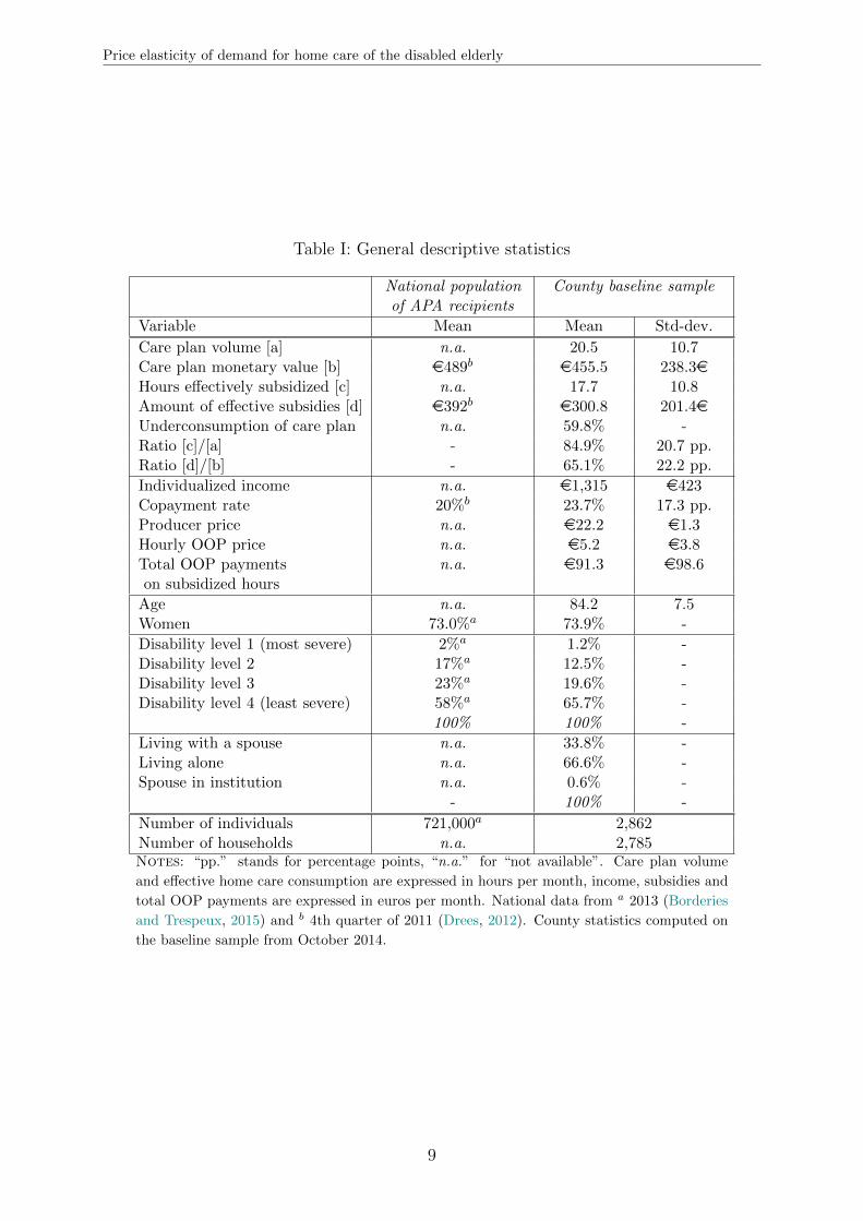
Table I describes the final sample used in the econometric analysis. Its
sociodemographic structure can be compared with national data on APA re-
cipients. The typical individual in our sample is a woman, in her mid-80s and
living alone, in line with the sociodemographic characteristics of the French
disabled elderly population. Strongly disabled individual are slightly less rep-
resented in our sample than at the national level. The average copayment rate
on APA is slightly higher than the national average, reflecting the fact that
individuals in our county tend to be richer. Six APA beneficiaries out of ten
do not consume the maximum number of hours for which they are entitled to
a subsidy; price sensitivity of the disabled elderly is one possible candidate to
explain part of this high figure.
[Table I (p. 9) about here]
3.4 A censored measure of home care consumption
The dataset contains the individual number of home care hours that are
charged by the producer to the CC or, equivalently, the subsidized hours of
home care. However, we do not observe the total volume of home care con-
sumed by each APA beneficiary, who is free to consume home care beyond
her care plan volume. For 40% of our sample, our measure of home care con-
sumption is then possibly right–censored. Appropriate econometric methods
are needed.
8
Price elasticity of demand for home care of the disabled elderly
Table I: General descriptive statistics
National populationof APA recipients
County baseline sample
Variable Mean Mean Std-dev.
Care plan volume [a] n.a. 20.5 10.7Care plan monetary value [b] e489b e455.5 238.3eHours effectively subsidized [c] n.a. 17.7 10.8Amount of effective subsidies [d] e392b e300.8 201.4eUnderconsumption of care plan n.a. 59.8% -Ratio [c]/[a] - 84.9% 20.7 pp.Ratio [d]/[b] - 65.1% 22.2 pp.
Individualized income n.a. e1,315 e423Copayment rate 20%b 23.7% 17.3 pp.Producer price n.a. e22.2 e1.3Hourly OOP price n.a. e5.2 e3.8Total OOP payments n.a. e91.3 e98.6on subsidized hours
Age n.a. 84.2 7.5Women 73.0%a 73.9% -
Disability level 1 (most severe) 2%a 1.2% -Disability level 2 17%a 12.5% -Disability level 3 23%a 19.6% -Disability level 4 (least severe) 58%a 65.7% -
100% 100% -
Living with a spouse n.a. 33.8% -Living alone n.a. 66.6% -Spouse in institution n.a. 0.6% -
- 100% -
Number of individuals 721,000a 2,862Number of households n.a. 2,785Notes: “pp.” stands for percentage points, “n.a.” for “not available”. Care plan volume
and effective home care consumption are expressed in hours per month, income, subsidies and
total OOP payments are expressed in euros per month. National data from a 2013 (Borderies
and Trespeux, 2015) and b 4th quarter of 2011 (Drees, 2012). County statistics computed on
the baseline sample from October 2014.
9

Price elasticity of demand for home care of the disabled elderly
4 EMPIRICAL STRATEGY
4.1 Econometric specification
Denote hi the number of home care hours billed to the CC for beneficiary i.
Only effectively–consumed hours can be billed, and this within the limit of the
care plan volume hi. Thus, hi ≤ h∗i and hi ≤ hi. If the individual consumes
less than the care plan volume, the consumption registered by the CC is equal
to her effective consumption (hi = h∗i if h∗i ≤ hi): there is no censoring issue.
If the individual consumes more than the care plan volume, the consumption
registered by the CC will systematically be equal to her individual ceiling
(hi = hi if h∗i > hi). Consequently, when hi = hi is observed, we either have
h∗i = hi, or h∗i > hi (right-censored consumption).
The estimation of the parameters of the demand function g(.) can only
rely on information relating to the first segment of the budget constraint. For
individuals consuming hi or more, the only information we can use is that
g(cipi, Ii;Xi) + νi > hi, whether i is exactly at the kink or actually consumes
more than hi.7 The observed consumption of home care rewrites as:{hi = g(cipi, Ii;Xi) + νi if g(cipi, Ii;Xi) + νi < hi
hi = hi if g(cipi, Ii;Xi) + νi ≥ hi(2)
Given that the distribution of home care consumption is slightly skewed,
we assume a log-linear specification of g(cipi, Ii;Xi) + νi:
ln(h∗i ) = β0 + β1.ln(cipi) + β2.ln(Ii) +X ′i.θ + εi
Both the consumer price and income are included in log so that β1 repre-
sents the consumer price elasticity and β2 represents the income elasticity of
the uncompensated demand for home care service.
In the data, the record of disposable income is not the current value of
income, but the income when the copayment rate was computed or last revised,
denoted Iobsi . We express current disposable income as: Ii = Iobsi γi, with γi the
rate of increase of individual disposable income since i’s last copayment rate
was computed. As the rate of increase in disposable income γi is not directly
observable, we write:
ln(h∗i ) = β0 + β1.ln(cipi) + β2.ln(Iobsi ) +2014∑
d=2009
λd.1di +X ′i.θ + εi (3)
7Appendix C provides more details.
10

Price elasticity of demand for home care of the disabled elderly
where 1di is a dummy equal to one when i’s copayment rate was last revised
in year d (1d, d = 2009, ..., 2014) and coefficients λd should capture the rate of
increase in income since year d.8
Together with the observational scheme summed up by System (2), Equa-
tion (3) corresponds to a censored regression model. Estimation of parameters
β and θ is done by Maximum Likelihood, after making the following paramet-
ric assumption:
ε | pi, Iobs, X, 1 ∼ N (0, σ2). (4)
4.2 Identification using cross-sectional variations in prices
Variations in the consumer price cipi come from a variation either in the
producer price pi or in the copayment rate ci that directly depends on the
disposable income IDi . As we control for disposable income, any variation in
the consumer price arises from a variation in the producer price. The consumer
price elasticity of demand is thus identified by the cross-sectional variation in
producer prices.9 In 2014, there are 27 producers in the county, offering 23
different prices. Producer prices range from e19.7 to e23.5, with an average
of e22.2 and a standard-deviation of e1.3.
For our estimation to give unbiased coefficients, the producer price charged
to individual i must be uncorrelated with the unobserved factors affecting
her home care consumption, εi. Supply-demand simultaneity may violate this
condition (Zhen et al., 2014), but it should be negligible with our data. Indeed,
each producer is priced by the CC on the basis of its average production cost
two years earlier and the pricing process largely depends on administrative
and political considerations (Gramain and Xing, 2012).
Omitted variables could also bias our estimation. Beneficiaries may non-
randomly select their producer (price) on the basis of some unobservable in-
dividual characteristics such as quality expectations, unobserved health con-
dition or informal care provision (Billaud et al., 2012). Although we can doc-
ument some sources of price variations, unlikely to be correlated with unob-
served determinants of home care consumption (Appendix D), it is insufficient
to rule out any price endogeneity induced by non–random producer choice.
To address this issue empirically, we make use of the unequal distribu-
tion of producers over space in the county. We divide our sample into two
8We implicitly assume the rate of increase in disposable income to be identical for two individualswhose personalized plans were decided upon the same year d. Retirees’ income is mostly made of pensionbenefits (Deloffre, 2009), which are reevaluated every year following the inflation rate. It remains a strongassumption given the heterogeneity in income composition across the income distribution.
9Appendix B provides more details on identification.
11

Price elasticity of demand for home care of the disabled elderly
sub–populations (Figure 2): on the one side, beneficiaries living in a munic-
ipality where a single producer is found to operate, or single–producer area
denoted “SPA” (areas in plain color). On the other hand, individuals living
in a municipality where two or more authorized producers have customers, or
non single–producer area denoted “non-SPA” (dotted areas). Selection into a
producer should be negligible in the first sub–sample (35% of baseline sample)
while it may arise in the second (65%).
Figure 2: Distribution of producers in the county – Schematic representation
Notes: We provide only a schematic representation to preserve the anonymityof the CC our data come from. Different shades of plain grey indicate differentareas served by a unique authorized service (single–producer areas, or SPA),each being served by a different producer with a given price level. The dottedareas correspond to multiple–producer municipalities, or non–SPA.
Overall, the two sub–samples do not differ in terms of consumption and
explaining observables (Appendix D). Living in a SPA does not affect signif-
icantly home care consumption nor its estimated price elasticity. Estimating
our model on the two sub–samples can then be interpreted as a test of price
endogeneity.
12

Price elasticity of demand for home care of the disabled elderly
5 RESULTS AND DISCUSSION
5.1 Main results
As we estimate a censored regression model, the coefficients displayed in
the tables give the predicted impact of a marginal (or 0/1) change in a given
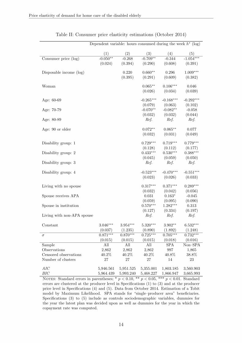
explaining variable on the total, uncensored home care consumption. Table II
presents our baseline results, obtained on the data from 2014. Column (1) does
not include sociodemographic controls, while the others do. Estimations (1) to
(3) are run on the entire sample while Estimations (4) and (5) are respectively
run on the subsamples of SPA beneficiaries and non–SPA beneficiaries. With
the entire sample, standard errors are clustered at the producer level to deal
with potential correlation across the error terms of observations with the same
producer. With subsamples, standard errors are clustered at the (producer)
price level, as the construction of the two subsamples artificially increases the
empirical variance in prices.
[Table II (p. 14 about here]
With no controls whatsoever, a 1% increase in the consumer price is associ-
ated with a very small variation of -0.05% in the hours of home care consumed.
Comparison of Specifications (1) and (2) evidences a negative correlation be-
tween income and producer price. The estimated coefficient increases (in abso-
lute value) to -0.709 when we include disposable income and sociodemographic
controls. The price elasticity coefficient is negative, statistically significant, in
Columns (3) and (4), suggesting that the disabled elderly are sensitive to the
consumer price of home care.
Restricting the sample to individuals who have no producer choice, the
point estimate of the price elasticity is reduced to around -0.34. Given the
smaller sample size and reduced identifying variation in prices, precision is low
and we cannot formally reject that the price elasticity is zero at conventional
statistical significance levels. The point estimate is higher when we run the
estimation on the subpopulation of individuals who can choose between differ-
ent providers: the estimator is significantly different from zero at the 1% level,
with a point value of -1.05. As the selection effect is inflationary, on average,
individuals willing to consume more hours go for relatively cheap services when
they can choose between several producers. This value thus captures what we
may call the overall price sensitivity of consumption, which includes both an
ex ante selection into a producer on the basis of expected consumption (“pay
less to consume more”) and the real price elasticity (“consuming more when
paying less”).
13
Price elasticity of demand for home care of the disabled elderly
Table II: Consumer price elasticity estimations (October 2014)
Dependent variable: hours consumed during the week h∗ (log)
(1) (2) (3) (4) (5)Consumer price (log) -0.050∗∗ -0.268 -0.709∗∗ -0.344 -1.054∗∗∗
(0.024) (0.394) (0.290) (0.608) (0.391)
Disposable income (log) 0.220 0.660∗∗ 0.296 1.009∗∗∗
(0.395) (0.291) (0.609) (0.382)
Woman 0.065∗∗ 0.106∗∗∗ 0.046(0.026) (0.034) (0.039)
Age: 60-69 -0.265∗∗∗ -0.168∗∗∗ -0.292∗∗∗
(0.079) (0.063) (0.102)Age: 70-79 -0.070∗∗ -0.082∗∗ -0.058
(0.032) (0.032) (0.044)Age: 80-89 Ref. Ref. Ref.
Age: 90 or older 0.072∗∗ 0.065∗∗ 0.077(0.032) (0.031) (0.049)
Disability group: 1 0.729∗∗∗ 0.719∗∗∗ 0.779∗∗∗
(0.128) (0.112) (0.177)Disability group: 2 0.433∗∗∗ 0.530∗∗∗ 0.388∗∗∗
(0.045) (0.059) (0.050)Disability group: 3 Ref. Ref. Ref.
Disability group: 4 -0.523∗∗∗ -0.470∗∗∗ -0.551∗∗∗
(0.023) (0.026) (0.033)
Living with no spouse 0.317∗∗∗ 0.371∗∗∗ 0.289∗∗∗
(0.032) (0.042) (0.056)Spouse receives APA 0.031 0.163∗ -0.045
(0.059) (0.095) (0.090)Spouse in institution 0.570∗∗∗ 1.282∗∗∗ 0.313
(0.127) (0.334) (0.197)Living with non-APA spouse Ref. Ref. Ref.
Constant 3.046∗∗∗ 3.954∗∗∗ 5.320∗∗∗ 3.902∗∗ 6.532∗∗∗
(0.037) (1.235) (0.890) (1.892) (1.248)σ 0.871∗∗∗ 0.870∗∗∗ 0.725∗∗∗ 0.705∗∗∗ 0.732∗∗∗
(0.015) (0.015) (0.015) (0.018) (0.016)Sample All All All SPA Non–SPAObservations 2,862 2,862 2,862 997 1,865Censored observations 40.2% 40.2% 40.2% 40.8% 38.8%Number of clusters 27 27 27 14 23
AIC 5,946.561 5,951.525 5,355.001 1,803.185 3,560.903BIC 5,964.439 5,993.240 5,468.227 1,866.947 3,665.993
Notes: Standard errors in parentheses; * p < 0.10, ** p < 0.05, *** p < 0.01. Standarderrors are clustered at the producer level in Specifications (1) to (3) and at the producerprice level in Specifications (4) and (5). Data from October 2014. Estimation of a Tobitmodel by Maximum Likelihood. SPA stands for “single–producer area” beneficiaries.Specifications (3) to (5) include as controls sociodemographic variables, dummies forthe year the latest plan was decided upon as well as dummies for the year in which thecopayment rate was computed.
14

Price elasticity of demand for home care of the disabled elderly
Turning to the effects of control variables, the marshallian income effect is
positive and inferior to 1 in our preferred estimation (Column (4)), though not
statistically significant. β2 captures the effect of an increase in income when
the copayment rate is fixed, which is likely to be the case in the short-run.
In the medium-run, any marginal increase in disposable income entails two
effects: (i) an income effect, through which the increase in the individual’s
budget set makes the consumption of all normal goods increase, (ii) a price
effect playing in the opposite direction, as an income increase will induce the
APA copayment rate to rise. Our estimations suggest that the overall effect of
an income change within the APA scheme, β1 + β2, is zero. Given the specific
schedule of APA copayments, the final impact of a marginal increase in the
OOP price within APA corresponds to the substitution effect.
As expected, the heavier the disability level, the higher the predicted con-
sumption, all other factors being equal. Even when controlling for disability
level, age retains a significant effect on the consumption on home care ser-
vices. Being a woman increases the consumption of professional home care by
a small but statistically significant amount. Living alone (spouse in institution
or no spouse) increases the amount of professional assistance received, consis-
tently with previous works showing the importance of the co-residing spouse
in providing informal care substituting partly for formal home care services.
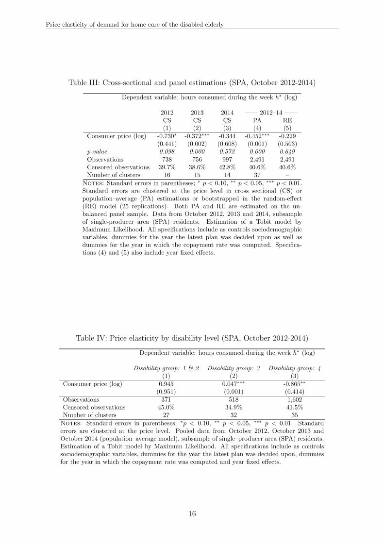
5.2 Further results and robustness checks
Table III gives the results of the estimations on SPA beneficiaries using
2012 and 2013 data. We also exploit the panel dimension of our data, by
estimating population-average and random-effect models on the pooled obser-
vations from 2012, 2013 and 2014 (same Table). Panel estimations increase
precision by providing an additional source of variation for identification: as
the administrated price of each producer is re-evaluated every year, we observe
some intra-individual variations in the producer price over time.10 Overall, fur-
ther results are consistent with our baseline cross-sectional estimates. Some
estimations even makes it possible to conclude to the significance of the price
elasticity estimator at the 1% level.
[Tables III and IV (p. 16) about here]
10On average, producer prices have increased by 1.9% between October 2012 and 2013 and by 1.3%between 2013 and 2014.
15
Price elasticity of demand for home care of the disabled elderly
Table III: Cross-sectional and panel estimations (SPA, October 2012-2014)
Dependent variable: hours consumed during the week h∗ (log)
2012 2013 2014 —— 2012–14 ——CS CS CS PA RE(1) (2) (3) (4) (5)
Consumer price (log) -0.730∗ -0.372∗∗∗ -0.344 -0.452∗∗∗ -0.229(0.441) (0.002) (0.608) (0.001) (0.503)
p-value 0.098 0.000 0.572 0.000 0.649Observations 738 756 997 2,491 2,491Censored observations 39.7% 38.6% 42.8% 40.6% 40.6%Number of clusters 16 15 14 37 –
Notes: Standard errors in parentheses; ∗ p < 0.10, ∗∗ p < 0.05, ∗∗∗ p < 0.01.Standard errors are clustered at the price level in cross–sectional (CS) orpopulation–average (PA) estimations or bootstrapped in the random-effect(RE) model (25 replications). Both PA and RE are estimated on the un-balanced panel sample. Data from October 2012, 2013 and 2014, subsampleof single-producer area (SPA) residents. Estimation of a Tobit model byMaximum Likelihood. All specifications include as controls sociodemographicvariables, dummies for the year the latest plan was decided upon as well asdummies for the year in which the copayment rate was computed. Specifica-tions (4) and (5) also include year fixed effects.
Table IV: Price elasticity by disability level (SPA, October 2012-2014)
Dependent variable: hours consumed during the week h∗ (log)
Disability group: 1 & 2 Disability group: 3 Disability group: 4(1) (2) (3)
Consumer price (log) 0.945 0.047∗∗∗ -0.865∗∗
(0.951) (0.001) (0.414)Observations 371 518 1,602Censored observations 45.0% 34.9% 41.5%Number of clusters 27 32 35
Notes: Standard errors in parentheses; ∗p < 0.10, ∗∗ p < 0.05, ∗∗∗ p < 0.01. Standarderrors are clustered at the price level. Pooled data from October 2012, October 2013 andOctober 2014 (population–average model), subsample of single–producer area (SPA) residents.Estimation of a Tobit model by Maximum Likelihood. All specifications include as controlssociodemographic variables, dummies for the year the latest plan was decided upon, dummiesfor the year in which the copayment rate was computed and year fixed effects.
16

Price elasticity of demand for home care of the disabled elderly
To investigate the potential heterogeneity in price sensitivity, we estimate
the model on three subsamples corresponding to different disability levels (Ta-
ble IV). We find that the lower the disability level is, the higher the price sen-
sitivity. It echoes the findings of previous works showing that poorer health
status is associated with a lower price elasticity of healthcare consumption
(Fukushima et al., 2016). In addition, price sensitivity is found to increase
with income quartile (Appendix E.1).
Our Tobit model assumes the individual–specific censoring point is uncor-
related with the unobserved determinants of professional home care consump-
tion. It also relies on the homoscedasticity and normality of the error term.
We investigate the robustness of our results by estimating an alternative spec-
ification, using as the latent dependent variable the (log) ratio of home care
consumption relative to the personalized care plan, h∗i /hi. With a fixed cen-
soring point, this transformation opens the way for semi–parametric models.
Estimations by Tobit, Censored Least Absolute Deviation (Powell, 1984) and
censored quantile regressions (Chernozhukov et al., 2015) provide statistically
significant estimates ranging from -0.5 to -0.2, in line with our baseline results
(Appendices E.2 and E.3).
5.3 Discussion
Our results confirm that the consumption of home care of the disabled
elderly is sensitive to its OOP cost. Decisions relating to home care consump-
tion are influenced by a trade-off between the OOP price of an extra hour and
its marginal value. Such a pecuniary trade–off was highlighted at the exten-
sive margin, as the take–up of APA benefits is affected by the average subsidy
rate in the county (Arrighi et al., 2015). More originally, we find evidence
that the price elasticity of the demand for domestic help is seemingly lower
than unity at the intensive margin. This result is in line with the estimates of
the average price elasticity of demand of -0.5 and -0.15 respectively found by
Bourreau-Dubois et al. (2014) and Hege (2016). Home care services should be
regarded as necessary goods, in the sense that adjustment of consumption is
proportionally lower than a given change in price.
We retrieve the price elasticity of home care expenditures to compare our
results with estimates obtained in the literature on the demand for medical
services. Manning et al. (1987); Keeler and Rolph (1988) found a price elastic-
ity of medical spending of -0.2; although its magnitude is subject to discussion,
its negative sign was found to be robust (Aron-Dine et al., 2013). With a price
elasticity of demand of -0.4, the price elasticity of expenditures is positive: an
17

Price elasticity of demand for home care of the disabled elderly
increase in the unit OOP payment of formal care will lead to a less than pro-
portional decrease in consumption, and thus to an increase in OOP and total
expenditures.
Our OOP price measure does not take into account possible tax reduc-
tions on home care services, unobserved in the data. Given we lack sufficient
information to simulate them, we implicitly assume APA beneficiaries to be
sensitive to the “spot” price (Geoffard, 2000). We also assume that APA re-
cipients react in the same way to variations in the copayment rate and in the
producer price. If salience differs (Chetty et al., 2009), implications for the
design of the copayment schedule are less straightforward.
In our administrative data, information on family characteristics is poor.
Receiving more informal care has been found to decrease formal care use,
both at the extensive and intensive margins (Van Houtven and Norton, 2004;
Bonsang, 2009). Omitting informal care provision could bias the estimates of
our entire set of coefficients. As a robustness check, we include as a control
whether the individual receives formal home care during the weekend and
public holidays. We hypothesize that individuals not receiving care over the
weekend are more likely to receive assistance from their relatives. Receiving
home care during the weekend is associated with more hours consumed during
working days (Table E.I) but does not significantly affect the price elasticity
estimate.
[Table E.I (p. 44) about here]
Finally, external validity of our results should be qualified. Without data
covering the entire population eligible to APA, the potential bias induced
by the differential take–up of APA subsidies (Chauveaud and Warin, 2005)
cannot be dealt with. Our sample is not nationally representative and we
focus on APA recipients who consume home care from authorized services.
Yet the county was selected to be “average” in terms of socio-economic and
demographic characteristics. In addition, customers of authorized home care
services represent a large share of APA beneficiaries in France.
18

Price elasticity of demand for home care of the disabled elderly
Table V: Inclusion of home care received on weekends (SPA, October 2012-2014)
Dependent variable: hours consumed during the week h∗ (log)
(1) (2) (3)Consumer price (log) -0.452∗∗∗ -0.637∗∗∗ -0.604∗∗∗
(0.001) (0.001) (0.001)Consumes care on weekends 0.502∗∗∗ -0.095∗∗∗
(0.008) (0.008)Number of hours received on weekends 0.189∗∗∗
(0.002)Observations 2,491 2,491 2,491Censored observations 40.6% 40.6% 40.6%Number of clusters 37 37 37
AIC 4,454.546 4,389.963 4,364.021BIC 4,600.057 4,541.294 4,521.173
Notes: Standard errors in parentheses; ∗ p < 0.10, ∗∗ p < 0.05, ∗∗∗ p < 0.01.Standard-errors are clustered at the price level. Pooled data from October2012, 2013 and 2014 (population–average model), subsample of single–producerarea (SPA) residents. Estimation of a Tobit model by Maximum Likelihood.All specifications include as controls sociodemographic variables, dummies forthe year the latest plan was decided upon, dummies for the year in which thecopayment rate was computed and year fixed effects.The latent dependent variable is the number of hours consumed betweenMonday and Saturday, except for public holidays. APA beneficiaries may alsoreceive a subsidy for a few hours of care to be received during weekends andpublic holidays, which are set separately in the personalized care plan. Wedid not include the home care hours received on weekends as a control in ourbaseline specifications because of a simultaneity concern. Only 7.5% of ourbaseline sample has weekend hours included in her personalized care plan, fora median volume of about 5 hours a month.
19
Price elasticity of demand for home care of the disabled elderly
6 CONCLUSION
This paper estimates the consumer price elasticity of the demand for home
care services of the disabled elderly living in the community and benefiting
from the French APA program. Our results suggest this parameter is, in abso-
lute value, inferior to one. Although the significance at conventional thresholds
is not systematic, the point estimate of -0.4 we obtain is roughly stable across
estimations.
Our findings pave the way for several public policy implications. As the
disabled elderly are sensitive to the price of care, the copayment rates in home
care subsidies programs entail allocative and dynamic efficiency issues. The
specific schedule of APA copayments makes the price elasticity we estimate a
sufficient statistics for the substitution effect in home care subsidy schemes.
Given the low value of the price elasticity (among the most severely disabled
individuals notably), the generosity of home care subsidies also has substan-
tial redistributive effects from taxpayers to the disabled elderly. In the case of
APA, the linear copayment schedule actually cancels out the effect of recipi-
ents’ income on home care consumption. Our estimates can also be used to
discuss the effects of potential reforms of home care subsidies. The decrease of
copayment rates planned by the 2016 APA reform, higher for more–disabled
recipients, should reduce beneficiaries’ overall OOP expenses on professional
home care, while having little volume effect on current APA recipients.
Finally, our study points out the unequal access to home care services
over the territory. Individuals living in municipalities with a unique producer
cannot choose their producer, on the basis of price or other characteristics such
as quality or weekend service. It evidences the need for further development
on spatial equity in access to home care services.
20
Price elasticity of demand for home care of the disabled elderly
Funding and acknowledgments
This research was carried out within the MODAPA project, which aims
at studying the determinants of long–term care utilization in France (more
information at: www.modapa.cnrs.fr). It was supported by a research grant
from the Agence nationale de la recherche (ANR) (ANR-14-CE30-0008) and
benefited from the joint support of Direction Generale de la Sante (DGS),
Mission recherche de la Direction de la recherche, des etudes, de l’evaluation
et des statistiques (MiRe-DREES), Caisse Nationale d’Assurance Maladie des
Travailleurs Salaries (CNAMTS), Regime Social des Independants (RSI) and
Caisse Nationale de Solidarite pour l’Autonomie (CNSA), within the call for
projets launched by the Institut de recherche en sante publique (IRESP) in
2013.
We are grateful to an anonymous French County Council (Conseil departemental)
for granting the access to its data and to Fondation Mederic Alzheimer for the
generous support provided to Marianne Tenand’s doctoral research.
21

Price elasticity of demand for home care of the disabled elderly
References
Aron-Dine A., Einav L., Finkelstein A. 2013. The RAND Health Insurance Experiment,
Three Decades Later. Journal of Economic Perspectives 27(1): 197–222.
Arrighi Y., Davin B., Trannoy A., Ventelou B. 2015. The non-take up of long-term care
benefit in France: A pecuniary motive?. Health Policy 119(10): 1338–1348.
Barnay T., Juin S. 2016. Does home care for dependent elderly people improve their mental
health?. Journal of Health Economics 45: 149–160.
Billaud S., Bourreau-Dubois C., Gramain A., Lim H., Weber F., Xing J. 2012. La prise
en charge de la dependance des personnes agees: les dimensions territoriales de l’action
publique. Rapport final realise pour la MiRe/Drees.
Blanpain N., Chardon O. 2010. Projections de population a l’horizon 2060 : un tiers de la
population agee de plus de 60 ans. INSEE Premiere (1320).
Bonsang E. 2009. Does informal care from children to their elderly parents substitute for
formal care in Europe?. Journal of Health Economics 28(1): 143–154.
Borderies F., Trespeux F. 2015. Les beneficiaires de l’aide sociale departementale en 2013.
Document de travail, Serie Statistiques 196. Drees.
Bourreau-Dubois C., Gramain A., Lim H., Xing J. 2014. Impact du reste a charge sur le
volume d’heures d’aide a domicile utilise par les beneficiaires de l’APA. CES Working
Paper 2014.24. Centre d’Economie de la Sorbonne.
Chauveaud C., Warin P. 2005. Des personnes agees hors leurs droits. Non recours subi ou
volontaire. Rencontres avec des assistantes sociales. Etude 11. Odenore. Grenoble.
Chernozhukov V., Fernandez-Val I., Kowalski A. E. 2015. Quantile regression with censoring
and endogeneity. Journal of Econometrics 186(1): 201–221.
Chernozhukov V., Hong H. 2002. Three-Step Censored Quantile Regression and Extramar-
ital Affairs. Journal of the American Statistical Association 97(459): 872–882.
Chetty R., Looney A., Kroft K. 2009. Salience and Taxation: Theory and Evidence. Amer-
ican Economic Review 99(4): 1145–1177.
Colombo F., Llena-Nozal A., Mercier J., Tjadens F. 2011. Help wanted ? Providing and Pay-
ing for Long-Term Care. OECD Health Policy Studies. OECD Publishing edn. OECD.
Paris.
Coughlin T. A., McBride T. D., Perozek M., Liu K. 1992. Home care for the disabled elderly:
predictors and expected costs. Health Services Research 27(4): 453–479.
Deloffre A. 2009. Les retraites en 2007. Document de travail, Serie Etudes et Recherches 86.
Drees.
Drees 2012. Enquete sur l’allocation personnalisee d’autonomie realisee par la Drees aupres
des conseils generaux. APA - Resultats de l’enquete trimestrielle 1. Drees.
22
Price elasticity of demand for home care of the disabled elderly
Drees 2015. Enquete annuelle Aide sociale aupres des conseils departementaux 2013.
Drees 2016. Enquete annuelle Aide sociale aupres des conseils departementaux 2014.
Ettner S. L. 1994. The Effect of the Medicaid Home Care Benefit On long-Term Care
Choices of the Elderly. Economic Inquiry 32(1): 103–127.
Fizzala A. 2016. Dependance des personnes agees : qui paie quoi ? L’apport du modele
Autonomix. Les dossiers de la Drees 1. Drees.
Fontaine R. 2012. The effect of public subsidies for formal care on the care provision for
disabled elderly people in france. Economie publique/Public Economics (28-29): 271–304.
Fukushima K., Mizuoka S., Yamamoto S., Iizuka T. 2016. Patient cost sharing and medical
expenditures for the Elderly. Journal of Health Economics 45: 115–130.
Geoffard P.-Y. 2000. Depenses de sante : l’hypothese d’alea moral. Economie et prevision
142(1): 122–135.
Gramain A., Xing J. 2012. Tarification publique et normalisation des processus de produc-
tion dans le secteur de l’aide a domicile pour les personnes agees. Revue francaise des
affaires sociales 2-3(2): 218–243.
Hege R. 2016. La demande d’aide a domicile est-elle sensible au reste-a-charge : une analyse
multi-niveaux sur donnees francaises. CES Working Paper 2016.22. Centre d’economie
de la Sorbonne.
Insee 2013. Populations legales 2011 des departements et des collectivites d’outre-mer.
URL: http://www.insee.fr/fr/ppp/bases-de-donnees/recensement/populations-
legales/france-departements.asp?annee=2011
Insee 2014. Estimations de population 2012.
URL: http://www.insee.fr/fr/themes/tableau.asp?regid = 0refid = NATnon02150
Insee-DGFiP-Cnaf-Cnav-Ccmsa 2015. Fichier localise social et fiscal (FiLoSoFi) 2012.
Keeler E. B., Rolph J. E. 1988. The demand for episodes of treatment in the Health Insurance
Experiment. Journal of Health Economics 7(4): 337–367.
Laferrere A., Angelini V. 2010. La mobilite residentielle des seniors en Europe. Retraite et
societe (2): 87–107.
Manning W. G., Newhouse J. P., Duan N., Keeler E. B., Leibowitz A., Maquis S. M.
1987. Health Insurance and the Demand for Medical Care: Evidence from a Randomized
Experiment. American Economic Review 77(3): 251–77.
Moffitt R. 1986. The Econometrics of Piecewise-Linear Budget Constraints: A Survey and
Exposition of the Maximum Likelihood Method. Journal of Business & Economic Statis-
tics 4(3): 317–328.
Moffitt R. 1990. The Econometrics of Kinked Budget Constraints. The Journal of Economic
Perspectives 4(2): 119–139.
23

Price elasticity of demand for home care of the disabled elderly
Pezzin L. E., Kemper P., Reschovsky J. 1996. Does Publicly Provided Home Care Substitute
for Family Care? Experimental Evidence with Endogenous Living Arrangements. The
Journal of Human Resources 31(3): 650–676.
Poletti B. 2012. Mission relative aux difficultes financieres de l’aide a domicile et aux
modalites de tarification et d’allocation de ressources des services d’aide a domicile pour
publics fragiles. Mission confiee par Madame Roselyne Bachelot-Narquin, Ministre des
Solidarites et de la Cohesion Sociale.
Powell J. L. 1984. Least absolute deviations estimation for the censored regression model.
Journal of Econometrics 25(3): 303–325.
Powell J. L. 1986. Censored regression quantiles. Journal of Econometrics 32(1): 143–155.
Rapp T., Chauvin P., Sirven N. 2015. Are public subsidies effective to reduce emergency
care? Evidence from the PLASA study. Social Science & Medicine 138: 31–37.
Rapp T., Grand A., Cantet C., Andrieu S., Coley N., Portet F., Vellas B. 2011. Public
financial support receipt and non-medical resource utilization in Alzheimer’s disease -
results from the PLASA study. Social Science & Medicine 72(8): 1310–1316.
Sieurin A., Cambois E., Robine J.-M. 2011. Les esperances de vie sans incapacite en France:
une tendance recente moins favorable que dans le passe. Document de travail 170. Ined.
Solard G. 2015. Les retraites et les retraites - Edition 2015. Collection Etudes et Statistiques.
Drees.
Stabile M., Laporte A., Coyte P. C. 2006. Household responses to public home care pro-
grams. Journal of Health Economics 25(4): 674–701.
Van Houtven C. H., Norton E. C. 2004. Informal care and health care use of older adults.
Journal of Health Economics 23(6): 1159–1180.
Vanlerenberghe J.-M., Watrin D. 2014. Rapport d’information fait au nom de la commission
des affaires sociales sur l’aide a domicile. Rapport d’information 575. Senat.
Zhen C., Finkelstein E. A., Nonnemaker J., Karns S., Todd J. E. 2014. Predicting the Effects
of Sugar-Sweetened Beverage Taxes on Food and Beverage Demand in a Large Demand
System. American Journal of Agricultural Economics 96(1): 1–25.
24

Price elasticity of demand for home care of the disabled elderly
APPENDICES
A CONSTRUCTION OF THE SAMPLE
A.1 Sample selection
This Appendix aims at documenting the selection steps our initial dataset
has gone through. For October 2014, administrative records indicate that
5,549 beneficiaries were receiving APA; but for 63 individuals, essential infor-
mation on subsidized hours, copayment rates or covariates was missing. These
individuals are presumably former APA recipients not yet erased from the files,
so we dropped them from our sample. The total number of beneficiaries is
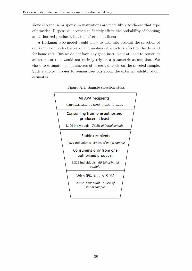
thus 5,486. Figure A.1 sums up the selection steps.
To observe precisely both the out-of-pocket price and the number of hours
that are effectively consumed and subsidized, we retain the beneficiaries re-
ceiving care from an authorized producer. They represent the majority of
APA recipients in the district (more than 4/5).
We then dropped the observations with missing information for the current
month, the preceding month or the following month to avoid potential unob-
servable shocks likely to bias our estimations. Indeed, missing information
could be related to temporary absences (like hospitalizations) or temporary
disruptions (e.g. visits from relatives, who replace temporarily professional
home care services by providing informal care). The remaining individuals
can be regarded as “stable”.
8 individuals receive home care from several producers at the same time.
If taken into account, the simultaneity of home care consumption decisions
for these individuals would make our empirical strategy considerably more
complex. We prefer to drop them. In addition, so as to make the relationship
between the consumer price and the producer price fully linear in disposable
income (see Appendix B), we retain only those individuals with a copayment
rate strictly between 0 and 90%.
We end up with a sample that represents 52% of total APA recipients of the
district. We follow the same steps to construct the samples of October 2012
and 2013. Percentages of individuals selected at each step are very similar to
what is found for 2014 and are available on request.
In order to assess the selection of our sample, we fit a Probit model ex-
plaining the probability to choose a authorized producer with the observable
characteristics. Results are displayed in Table A.I. Older individuals are less
likely to receive care from an authorized producer, while individuals living
25
Price elasticity of demand for home care of the disabled elderly
alone (no spouse or spouse in institution) are more likely to choose that type
of provider. Disposable income significantly affects the probability of choosing
an authorized producer, but the effect is not linear.
A Heckman-type model would allow to take into account the selection of
our sample on both observable and unobservable factors affecting the demand
for home care. But we do not have any good instrument at hand to construct
an estimator that would not entirely rely on a parametric assumption. We
chose to estimate our parameters of interest directly on the selected sample.
Such a choice imposes to remain cautious about the external validity of our
estimates.
Figure A.1: Sample selection steps
26

Price elasticity of demand for home care of the disabled elderly
Table A.I: Observable determinants of the choice of a authorized producer (October 2014)
Dependent variable: Served by an authorized producer
(1)Woman -0.001
(0.011)
Age: 60-69 0.019(0.024)
Age: 70-79 -0.014(0.014)
Age: 80-89 Ref.
Age: 90 or older -0.172∗∗∗
(0.011)
Disability level: 1 -0.063(0.039)
Disability level: 2 -0.014(0.017)
Disability level: 3 Ref.
Disability level: 4 0.011(0.013)
Living with no spouse 0.041∗∗∗
(0.012)Spouse receives APA 0.033
(0.030)Spouse in institution 0.202∗∗∗
(0.058)Living with non-APA spouse Ref.
Income quartile: 1 -0.045∗∗
(0.016)Income quartile: 2 Ref.
Income quartile: 3 -0.038∗∗
(0.015)Income quartile: 4 -0.134∗∗∗
(0.014)Observations 5,486Number of clusters 5,326
Notes: Standard errors in parentheses; ∗ p < 0.10, ∗∗ p < 0.05, ∗∗∗
p < 0.01. Standard errors are clustered at the household level. Thesample used correspond to all APA recipients in the District Councilin October 2014, except for individuals for which data on the copay-ment rate, on hours consumed or on sociodemographic characteris-tics were missing. Estimation is done by a probit model. Averagemarginal or partial effects (AME – APE) are displayed.
27

Price elasticity of demand for home care of the disabled elderly
A.2 Imputation of households
Although the data we collected indicate when a beneficiary lives with a
partner, we do not know whether the partner also receives APA. Having an
APA–recipient spouse may correlate with one’s own home care consumption;
failing to control for such a characteristic may bias our estimates.
To identify potential couples in our sample, we checked whether each indi-
vidual could be matched with another recipient of the opposite sex, recorded
as living with a spouse, with exactly the same income (as the APA copay-
ment schedule takes into account the household income) and residing in the
same municipality. If two individuals match, we assume they belong to the
same household. It allows us to construct both a dummy for residing with a
spouse receiving APA and a household identification number, which we use
when clustering standard errors at the household level (Table A.I).
The matching procedure may fail for individuals whose copayment rate
is 0%. The reported disposable income is the same for all such individuals,
be they actual spouses or not. The same pitfall applies for individuals whose
copayment rate is 90%. In October 2014, only 16 individuals were not matched
for this reason; this figure which should be small enough not to affect the
results presented in Table A.I. All other estimations rely on the sample of
individuals with a copayment rate strictly between 0 and 90%, for who the
matching procedure is systematically successful.
28
Price elasticity of demand for home care of the disabled elderly
B IDENTIFICATION
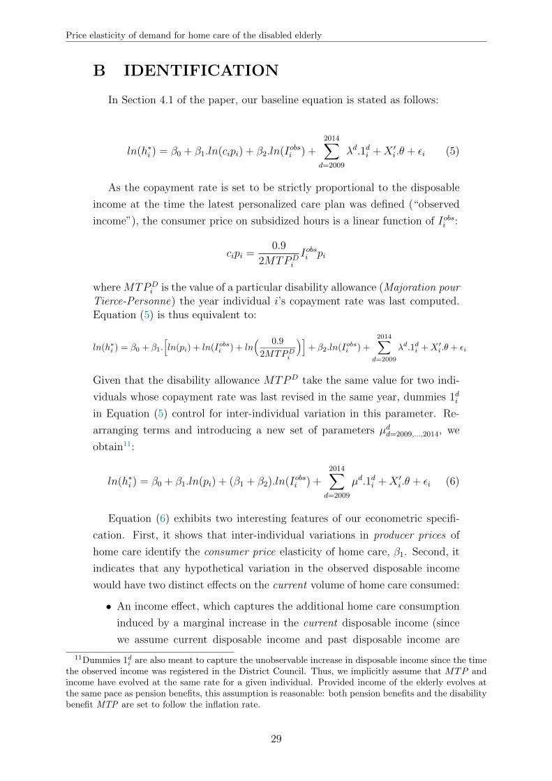
In Section 4.1 of the paper, our baseline equation is stated as follows:
ln(h∗i ) = β0 + β1.ln(cipi) + β2.ln(Iobsi ) +2014∑
d=2009
λd.1di +X ′i.θ + εi (5)
As the copayment rate is set to be strictly proportional to the disposable
income at the time the latest personalized care plan was defined (“observed
income”), the consumer price on subsidized hours is a linear function of Iobsi :
cipi =0.9
2MTPDi
Iobsi pi
where MTPDi is the value of a particular disability allowance (Majoration pour
Tierce-Personne) the year individual i’s copayment rate was last computed.Equation (5) is thus equivalent to:
ln(h∗i ) = β0 + β1.[ln(pi) + ln(Iobsi ) + ln
( 0.9
2MTPDi
)]+ β2.ln(Iobsi ) +
2014∑d=2009
λd.1di +X ′i.θ + εi
Given that the disability allowance MTPD take the same value for two indi-
viduals whose copayment rate was last revised in the same year, dummies 1di
in Equation (5) control for inter-individual variation in this parameter. Re-
arranging terms and introducing a new set of parameters µdd=2009,...,2014, we
obtain11:
ln(h∗i ) = β0 + β1.ln(pi) + (β1 + β2).ln(Iobsi ) +2014∑
d=2009
µd.1di +X ′i.θ + εi (6)
Equation (6) exhibits two interesting features of our econometric specifi-
cation. First, it shows that inter-individual variations in producer prices of
home care identify the consumer price elasticity of home care, β1. Second, it
indicates that any hypothetical variation in the observed disposable income
would have two distinct effects on the current volume of home care consumed:
• An income effect, which captures the additional home care consumption
induced by a marginal increase in the current disposable income (since
we assume current disposable income and past disposable income are
11Dummies 1di are also meant to capture the unobservable increase in disposable income since the timethe observed income was registered in the District Council. Thus, we implicitly assume that MTP andincome have evolved at the same rate for a given individual. Provided income of the elderly evolves atthe same pace as pension benefits, this assumption is reasonable: both pension benefits and the disabilitybenefit MTP are set to follow the inflation rate.
29

Price elasticity of demand for home care of the disabled elderly
mechanically related);
• A price effect, as any change in the disposable income induces a change in
the current individual consumer price when there is a new personalized
care plan.
In order to obtain directly the standard errors associated with the estimator
of coefficient β2, (6) can be written alternatively as:
ln(h∗i ) = β0 + β1.[ln(pi) + ln(Iobsi )
]+ β2.ln(Iobsi ) +
2014∑d=2009
µd.1di +X ′i.θ+ εi (7)
Compared to Equation (5), Equations (6) or (7) are less sensitive to the
measurement errors on the relationship between income and consumer price.
For 2% of our sample, the relationship between the income and the copayment
rate does not verify the legal formula used to compute the copayment rate.12
After a careful examination of the data, we hypothesize that most of these
errors occurred when the copayment rate was computed while the values of
income and copayment rate are assumed to be the real ones. It is then worthy
–in terms of precision gained– to include the corresponding observations in
the estimation. We add a dummy variable 1ei signaling whether the individual
is affected by such a calculation error.
To sum it up, in order to take into account the various subtleties of the
APA policy and the measurement errors, the true estimated equation is thus:
ln(h∗i ) = β0 +β1.[ln(pi)+ ln(Iobsi )
]+β2.ln(Iobsi )+
2014∑d=2009
µd.1di + ζ.1e
i +X ′i.θ+ εi
12In practical terms, we are not able to retrieve the value of the MTP related to the year in which thecopayment rate was officially computed; as a consequence, for those individuals, all dummies 1d take thevalue of zero.
30
Price elasticity of demand for home care of the disabled elderly
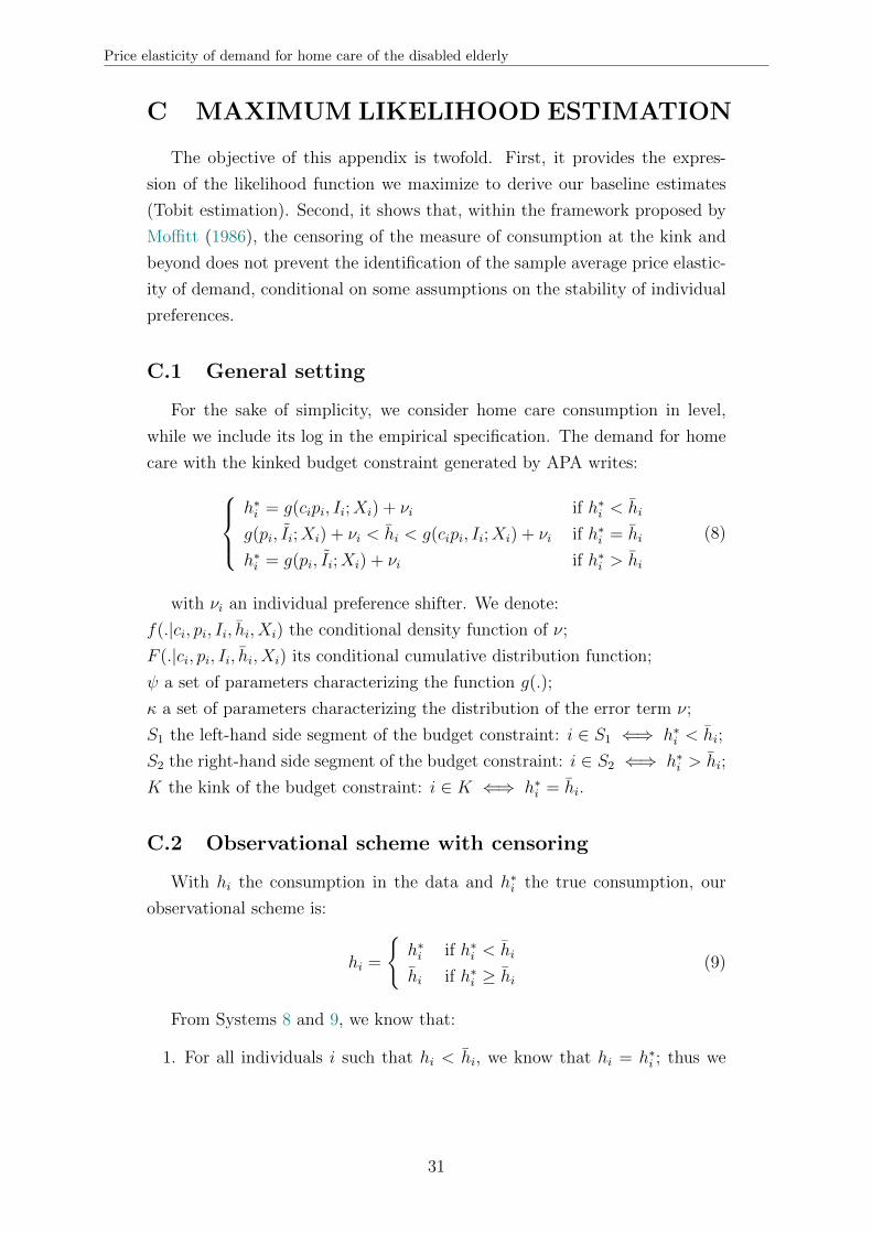
C MAXIMUM LIKELIHOOD ESTIMATION
The objective of this appendix is twofold. First, it provides the expres-
sion of the likelihood function we maximize to derive our baseline estimates
(Tobit estimation). Second, it shows that, within the framework proposed by
Moffitt (1986), the censoring of the measure of consumption at the kink and
beyond does not prevent the identification of the sample average price elastic-
ity of demand, conditional on some assumptions on the stability of individual
preferences.
C.1 General setting
For the sake of simplicity, we consider home care consumption in level,
while we include its log in the empirical specification. The demand for home
care with the kinked budget constraint generated by APA writes:h∗i = g(cipi, Ii;Xi) + νi if h∗i < hi
g(pi, Ii;Xi) + νi < hi < g(cipi, Ii;Xi) + νi if h∗i = hi
h∗i = g(pi, Ii;Xi) + νi if h∗i > hi
(8)
with νi an individual preference shifter. We denote:
f(.|ci, pi, Ii, hi, Xi) the conditional density function of ν;
F (.|ci, pi, Ii, hi, Xi) its conditional cumulative distribution function;
ψ a set of parameters characterizing the function g(.);
κ a set of parameters characterizing the distribution of the error term ν;
S1 the left-hand side segment of the budget constraint: i ∈ S1 ⇐⇒ h∗i < hi;
S2 the right-hand side segment of the budget constraint: i ∈ S2 ⇐⇒ h∗i > hi;
K the kink of the budget constraint: i ∈ K ⇐⇒ h∗i = hi.
C.2 Observational scheme with censoring
With hi the consumption in the data and h∗i the true consumption, our
observational scheme is:
hi =
{h∗i if h∗i < hi
hi if h∗i ≥ hi(9)
From Systems 8 and 9, we know that:
1. For all individuals i such that hi < hi, we know that hi = h∗i ; thus we
31

Price elasticity of demand for home care of the disabled elderly
have h∗i < hi (i ∈ S1):
hi = g(cipi, Ii;Xi) + νi < hi
2. For individuals i such that hi = hi, we know that h∗i ≥ hi; these individ-
uals can be split in two different sub-groups:
(a) Individuals i such that h∗i = hi (i ∈ K); then:{g(cipi, Ii;Xi) + νi > hi
g(pi, Ii;Xi) + νi < hi
(b) Individuals i such that h∗i > hi (i ∈ S2); then:{g(cipi, Ii;Xi) + νi > hi
g(pi, Ii;Xi) + νi > hi
Thus, all censored observations (i ∈ S2 or i ∈ K) have in common the fact
that:
g(cipi, Ii;Xi) + νi ≥ hi
We can thus write:
hi =
{g(cipi, Ii;Xi) + νi if g(cipi, Ii;Xi) + νi < hi
hi if g(cipi, Ii;Xi) + νi ≥ hi(10)
which corresponds to the usual censored regression model setting.
C.3 The likelihood function with censoring
Let h be a random variable, from which hi is a random draw. Conditional
on the observable covariates, h = g(CPi, Ii;Xi) + ν, where ν is a normally
distributed random variable from which νi is a random draw. From System
10, we can derive the individual contributions to the likelihood function:
1. Contribution of an individual i such that hi < hi (i ∈ S1):
P(hi = h∗i |ci, pi, Ii, Xi
)|h∗
i<hi= P
(ν = hi − g(cipi, Ii;Xi)|ci, pi, Ii, Xi
)= f
(hi − g(cipi, Ii;Xi)|ci, pi, Ii, Xi
)
32
Price elasticity of demand for home care of the disabled elderly
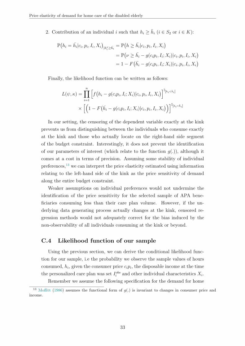
2. Contribution of an individual i such that hi ≥ hi (i ∈ S2 or i ∈ K):
P(hi = hi|ci, pi, Ii, Xi
)|h∗
i≥hi= P
(h ≥ hi|ci, pi, Ii, Xi
)= P
(ν ≥ hi − g(cipi, Ii;Xi)|ci, pi, Ii, Xi
)= 1− F
(hi − g(cipi, Ii;Xi)|ci, pi, Ii, Xi
)Finally, the likelihood function can be written as follows:
L(ψ, κ) =n∏
i=1
[f(hi − g(cipi, Ii;Xi)|ci, pi, Ii, Xi
)]I[hi<hi]
×[(
1− F(hi − g(cipi, Ii;Xi)|ci, pi, Ii, Xi
))]I[hi=hi]
In our setting, the censoring of the dependent variable exactly at the kink
prevents us from distinguishing between the individuals who consume exactly
at the kink and those who actually locate on the right-hand side segment
of the budget constraint. Interestingly, it does not prevent the identification
of our parameters of interest (which relate to the function g(.)), although it
comes at a cost in terms of precision. Assuming some stability of individual
preferences,13 we can interpret the price elasticity estimated using information
relating to the left-hand side of the kink as the price sensitivity of demand
along the entire budget constraint.
Weaker assumptions on individual preferences would not undermine the
identification of the price sensitivity for the selected sample of APA bene-
ficiaries consuming less than their care plan volume. However, if the un-
derlying data generating process actually changes at the kink, censored re-
gression methods would not adequately correct for the bias induced by the
non-observability of all individuals consuming at the kink or beyond.
C.4 Likelihood function of our sample
Using the previous section, we can derive the conditional likelihood func-
tion for our sample, i.e the probability we observe the sample values of hours
consumed, hi, given the consumer price cipi, the disposable income at the time
the personalized care plan was set Iobsi and other individual characteristics Xi.
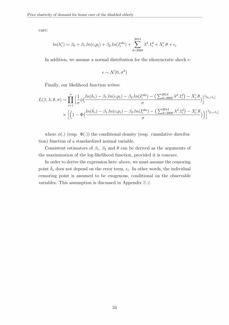
Remember we assume the following specification for the demand for home
13 Moffitt (1986) assumes the functional form of g(.) is invariant to changes in consumer price andincome.
33
Price elasticity of demand for home care of the disabled elderly
care:
ln(h∗i ) = β0 + β1.ln(cipi) + β2.ln(Iobsi ) +2014∑
d=2009
λd.1di +X ′i.θ + εi
In addition, we assume a normal distribution for the idiosyncratic shock ε:
ε ∼ N (0, σ2)
Finally, our likelihood function writes:
L(β, λ, θ, σ) =n∏
i=1
[ 1
σφ( ln(hi)− β1.ln(cipi)− β2.ln(Iobsi )−
(∑2014d=2009 λ
d.1di
)−X ′i.θ
σ
)]I[hi<hi]
×[(
1− Φ( ln(hi)− β1.ln(cipi)− β2.ln(Iobsi )−
(∑2014d=2009 λ
d.1di
)−X ′i.θ
σ
))]I[hi=hi]
where φ(.) (resp. Φ(.)) the conditional density (resp. cumulative distribu-
tion) function of a standardized normal variable.
Consistent estimators of β1, β2 and θ can be derived as the arguments of
the maximization of the log-likelihood function, provided it is concave.
In order to derive the expression here–above, we must assume the censoring
point hi does not depend on the error term, εi. In other words, the individual
censoring point is assumed to be exogenous, conditional on the observable
variables. This assumption is discussed in Appendix E.2.
34
Price elasticity of demand for home care of the disabled elderly
D SUPPLY BY AUTHORIZED PROVIDERS
D.1 Components of home care prices
In this section, we explain why customers may exogenously face different
producer prices: to do so, we detail the components of prices.
Authorized producers are priced by the County Countil (CC). The hourly
price of each producer is computed as the overall average hourly production
cost of the producer. The various components of production costs are de-
scribed in qualitative studies, either in academic works (Gramain and Xing,
2012) or in public reports.14 By order of importance (top–down), production
costs can be decomposed as follows:
[parsep=0.05cm,itemsep=0.05cm,topsep=0.05cm]Employee costs (80% of
total charges): wages paid to professional caregivers and, for a small part
(around 10% of total charges), to the supervising staff. The wage of
a caregiver depends on her qualification, according to collective labour
agreements. We expect that the larger the proportion of skilled care-
givers, the higher the production cost and the price. Wages are also
augmented if employees work on Sunday or on public holidays, in accor-
dance with general labour legislation. Operating costs (10–15% of total
charges): those include rents for the service’s offices and other running ex-
penses. Transportation costs (5–10% of total charges) correspond to the
compensation for the costs borne by employees to go to the consumer’s
home. This item is likely to vary largely across services according to
their geographic area of intervention. Contrary to the health care sector,
technological progress and capital costs are negligible in the home care
industry.
We represent the relationship between the producer price and several providers’
characteristics graphically. We distinguish between non–public (mainly non–
profit) producers and public producers. The latest are likely to receive grants
or advantages (e.g., a free office) from local municipalities that reduce operat-
ing costs. Such advantages are taken into account in the pricing process done
by the CC and lower down the regulated price of public producers. In the
graphical representation, we exclude the largest producer of the district, a na-
tionwide non–profit organization, which has systematically the highest values
for the variables we are here interested in.
In Figure D.1, producer prices are plot against the number of APA benefi-
14There is, though, no national, comprehensive benchmark study on the costs of home care services.Public reports regularly deplore the lack of information on costs as a major shortcoming preventing fromunderstanding the functioning of the sector (Vanlerenberghe and Watrin, 2014; Poletti, 2012).
35

Price elasticity of demand for home care of the disabled elderly
ciaries served by the corresponding services. Graphically, the more customers
the producer has, the higher its price. Having more customers might be associ-
ated with more municipalities to serve (see Figure D.3) or more unproductive
hours.15 This graph should be interpreted cautiously though: we only know
the number of APA recipients served by each home care producer, instead of
the total number of customers (including non–APA beneficiaries) served in
the district.
Figure D.2 shows the relationship between the producer price and the share
of hours they serve on Sundays or on public holidays. Public producers have
a very low share of such hours, as most public services do not operate on
weekends and holidays. A higher share of hours made on holidays is associated
with a higher price among public structures, which is consistent with the
financial compensation of employees for working on public holidays.
Finally, Figure D.3 shows that the relationship between the price and the
number of municipalities served by the producer is actually increasing. Taking
into account the spatial distribution of municipalities could be a way to refine
the analysis, as it would reflect transportation costs more accurately.
Figure D.1: Producer price according to the number of APA beneficiaries served by theproducer, by status
Sample: Authorized home care producers of the district serving at leastone APA beneficiary in October 2014.Notes: The largest producer, which serves 43% of the APA beneficia-ries who receive care from an authorized producer in the district, is notincluded.
15Unproductive hours (meetings, training) may become relatively more numerous when a service getsrelatively large.
36

Price elasticity of demand for home care of the disabled elderly
Figure D.2: Producer price according to the share of the producer’s hours served onSundays and public holidays, by status
Sample: Authorized home care producers of the district serving at leastone APA beneficiary in October 2014.Notes: The largest producer, which does 1.80% of the home care hoursit provides on Sundays and holidays, is not included.
Figure D.3: Producer price according to the number of served municipalities, by status
Sample: Authorized home care producers of the district serving at leastone APA beneficiary in October 2014.Notes: The largest producer, which serves 199 municipalities, is notincluded.
37
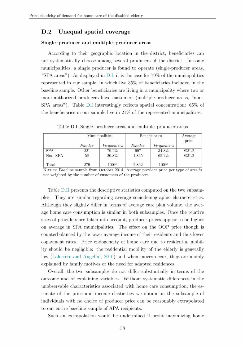
Price elasticity of demand for home care of the disabled elderly
D.2 Unequal spatial coverage
Single–producer and multiple–producer areas
According to their geographic location in the district, beneficiaries can
not systematically choose among several producers of the district. In some
municipalities, a single producer is found to operate (single-producer areas,
“SPA areas”). As displayed in D.I, it is the case for 79% of the municipalities
represented in our sample, in which live 35% of beneficiaries included in the
baseline sample. Other beneficiaries are living in a municipality where two or
more authorized producers have customers (multiple-producer areas, “non–
SPA areas”). Table D.I interestingly reflects spatial concentration: 65% of
the beneficiaries in our sample live in 21% of the represented municipalities.
Table D.I: Single–producer areas and multiple–producer areas
Municipalities Beneficiaries Averageprice
Number Frequencies Number FrequenciesSPA 221 79.2% 997 34.8% e21.2Non–SPA 58 20.8% 1,865 65.2% e21.2
Total 279 100% 2,862 100% -
Notes: Baseline sample from October 2014. Average provider price per type of area isnot weighted by the number of customers of the producers.
Table D.II presents the descriptive statistics computed on the two subsam-
ples. They are similar regarding average sociodemographic characteristics.
Although they slightly differ in terms of average care plan volume, the aver-
age home care consumption is similar in both subsamples. Once the relative
sizes of providers are taken into account, producer prices appear to be higher
on average in SPA municipalities. The effect on the OOP price though is
counterbalanced by the lower average income of their residents and thus lower
copayment rates. Price endogeneity of home care due to residential mobil-
ity should be negligible: the residential mobility of the elderly is generally
low (Laferrere and Angelini, 2010) and when moves occur, they are mainly
explained by family motives or the need for adapted residences.
Overall, the two subsamples do not differ substantially in terms of the
outcome and of explaining variables. Without systematic differences in the
unobservable characteristics associated with home care consumption, the es-
timate of the price and income elasticities we obtain on the subsample of
individuals with no choice of producer price can be reasonably extrapolated
to our entire baseline sample of APA recipients.
Such an extrapolation would be undermined if profit–maximizing home
38

Price elasticity of demand for home care of the disabled elderly
care producers willing to act as monopolies were targeting the municipalities
with no competitors and where residents are the least price–elastic. As ex-
plained further below, the home care providers are highly regulated: their
intervention area is defined by the CC. Moreover, they mostly come from the
non–profit organizations or from public municipal structures. It makes the as-
sumption that providers would choose their commercial area so as to extract
more profit quite unlikely.
Table D.II: Descriptive statistics on two subsamples (SPA and non SPA, October 2014)
••••
SPA Non–SPA P-value (diff.in means)
Variable (1) (2) (3)
Care plan volume 20.1 20.8 0.06Care plan monetary value e456.8 e454.8 0.83Hours effectively subsidized 17.5 17.8 0.37Amount of effective subsidies e311.7 e294.9 0.03Underconsumption of careplan volume
57.2% 61.2% 0.03
Individualized income e1,272 e1,339 0.00Copayment rate 21.9% 24.6% 0.00Producer price e22.8 e21.8 0.00Hourly out-of-pocket price e5.0 e5.4 0.01Total out-of-pocketpayments on subsidizedhours
e86.0 e94.2 0.03
Age 84.4 84.0 0.19Women 72.5% 74.7% 0.19Disability level 1 (mostsevere)
1.5% 1.0 % 0.25
Disability level 2 12.2% 12.6% 0.78Disability level 3 20.7% 19.1% 0.31Disability level 4 (leastsevere)
65.6% 67.3% 0.36
100% -Living with a spouse 34.7% 33.3% 0.45Living alone 64.7% 66.1% 0.45Spouse in institution 0.6% 0.6% 0.96
100% - -
Number of individuals 997 1,865 -Number of households 965 1,820 -
Notes: Baseline sample from October 2014. Descriptive statistics are computed on thesubsample of APA beneficiaries living in single–producer municipalities in Column (1) andthose living in multiple–producer municipalities in Column (2). Column (3) presents thep–values associated with the bilateral tests of comparison of the means.
39
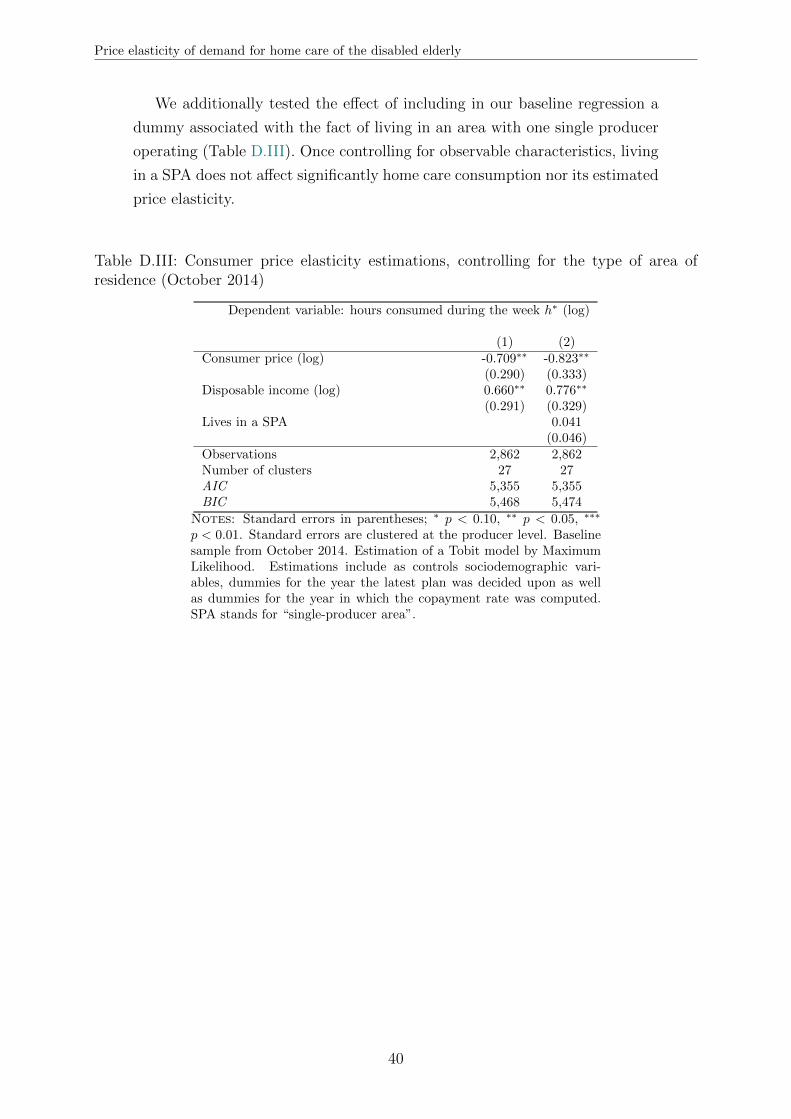
Price elasticity of demand for home care of the disabled elderly
We additionally tested the effect of including in our baseline regression a
dummy associated with the fact of living in an area with one single producer
operating (Table D.III). Once controlling for observable characteristics, living
in a SPA does not affect significantly home care consumption nor its estimated
price elasticity.
Table D.III: Consumer price elasticity estimations, controlling for the type of area ofresidence (October 2014)
Dependent variable: hours consumed during the week h∗ (log)
(1) (2)Consumer price (log) -0.709∗∗ -0.823∗∗
(0.290) (0.333)Disposable income (log) 0.660∗∗ 0.776∗∗
(0.291) (0.329)Lives in a SPA 0.041
(0.046)Observations 2,862 2,862Number of clusters 27 27AIC 5,355 5,355BIC 5,468 5,474
Notes: Standard errors in parentheses; ∗ p < 0.10, ∗∗ p < 0.05, ∗∗∗
p < 0.01. Standard errors are clustered at the producer level. Baselinesample from October 2014. Estimation of a Tobit model by MaximumLikelihood. Estimations include as controls sociodemographic vari-ables, dummies for the year the latest plan was decided upon as wellas dummies for the year in which the copayment rate was computed.SPA stands for “single-producer area”.
40
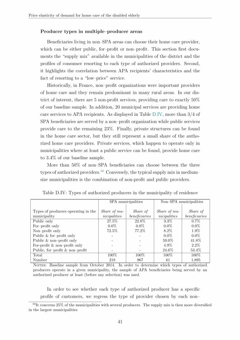
Price elasticity of demand for home care of the disabled elderly
Producer types in multiple–producer areas
Beneficiaries living in non–SPA areas can choose their home care provider,
which can be either public, for–profit or non–profit. This section first docu-
ments the “supply mix” available in the municipalities of the district and the
profiles of consumer resorting to each type of authorized providers. Second,
it highlights the correlation between APA recipients’ characteristics and the
fact of resorting to a “low–price” service.
Historically, in France, non–profit organizations were important providers
of home care and they remain predominant in many rural areas. In our dis-
trict of interest, there are 5 non-profit services, providing care to exactly 50%
of our baseline sample. In addition, 20 municipal services are providing home
care services to APA recipients. As displayed in Table D.IV, more than 3/4 of
SPA beneficiaries are served by a non–profit organization while public services
provide care to the remaining 23%. Finally, private structures can be found
in the home care sector, but they still represent a small share of the autho-
rized home care providers. Private services, which happen to operate only in
municipalities where at least a public service can be found, provide home care
to 3.4% of our baseline sample.
More than 50% of non–SPA beneficiaries can choose between the three
types of authorized providers.16 Conversely, the typical supply mix in medium–
size municipalities is the combination of non-profit and public providers.
Table D.IV: Types of authorized producers in the municipality of residence
SPA municipalities Non–SPA municipalities
Types of producers operating in themunicipality
Share of mu-nicipalities
Share ofbeneficiaries
Share of mu-nicipalities
Share ofbeneficiaries
Public only 27.5% 22.8% 3.3% 0.7%For–profit only 0.0% 0.0% 0.0% 0.0%Non–profit only 72.5% 77.2% 8.2% 1.9%Public & for–profit only - - 0.0% 0.0%Public & non–profit only - - 59.0% 41.8%For-profit & non–profit only - - 4.9% 2.2%Public, for–profit & non–profit - - 24.6% 53.4%Total 100% 100% 100% 100%Number 218 967 61 1,895
Notes: Baseline sample from October 2014. In order to determine which types of authorizedproducers operate in a given municipality, the sample of APA beneficiaries being served by anauthorized producer at least (before any selection) was used.
In order to see whether each type of authorized producer has a specific
profile of customers, we regress the type of provider chosen by each non–
16It concerns 25% of the municipalities with several producers. The supply mix is then more diversifiedin the largest municipalities
41

Price elasticity of demand for home care of the disabled elderly
SPA recipient on her individual characteristics. Columns (1), (2) and (3) of
Table D.V present the average impact of each observable characteristic on
the probability to be provided care by, respectively, a public, a for–profit or
a non–profit provider. The estimated coefficients should be regarded as the
distinctive characteristics of the subpopulation of customers of each producer
type. Indeed, 4 individuals out of 10 in the sample used for the estimation
can actually choose only between two different types of producers and we do
not control for any systematic difference in prices between producer types.
In our sample, the probability of choosing a public producer decreases
with high income, high disability level and week–end interventions. It might
be due to the fact that the operating hours and days of public services are
more restricted than the intervention schedules of private structures. The
probability of choosing a for–profit producer increases when the individual
belongs to the top income quartile income. Non–profit producers are more
likely to be chosen by highly–disabled individuals. The evaluation team may
tend to recommend them for the most severely disabled APA recipients who
will be likely to need interventions in the evening and during the weekend.
We also investigate the importance of the producer’s relative price in the
choice of a given home care provider. Column (4) of Table D.V presents the
individual characteristics associated with the choice of a “low–price” producer,
defined as a provider charging a price strictly below the average price charged
by the producers operating in the beneficiary’s municipality. We estimate the
probability of choosing a “low–price” producer by a Probit, on the sample of
individuals who live in a non–SPA municipality. Beyond a slight age effect,
only the disability level is found to have a significant impact. The least severely
disabled are more likely to choose a “low–price” producer, possibly reflecting
that they perceive home care as less necessary and are thus ex ante more
sensitive to its price.
42

Table D.V: Determinants of producer type for non–SPA beneficiaries (2012–2014)
Probability of choosing a:
Public For–profit Non–profit “Low–price”producer producer producer producer
——— Multinomial logit ——— — Probit —(1) (2) (3) (4)
Woman 0.023 -0.001 -0.022 -0.033(0.018) (0.005) (0.017) (0.020)
Age: 60-69 -0.141∗∗∗ 0.078∗∗ 0.063∗ -0.053(0.040) (0.035) (0.036) (0.053)
Age: 70-79 -0.089∗∗∗ 0.018∗ 0.071∗∗∗ -0.040∗
(0.019) (0.010) (0.020) (0.021)Age: 80-89 Ref. Ref. Ref. Ref.
Age: 90 or older -0.008 -0.008 0.017 -0.031(0.025) (0.006) (0.021) (0.023)
Disability group: 1 -0.230∗∗ 0.051 0.179∗∗ -0.120(0.091) (0.063) (0.075) (0.096)
Disability group: 2 -0.004 -0.015∗ 0.018 -0.033(0.039) (0.009) (0.035) (0.033)
Disability group: 3 Ref. Ref. Ref. Ref.
Disability group: 4 0.065∗∗ 0.024 -0.089∗∗∗ 0.085∗∗∗
(0.023) (0.018) (0.022) (0.021)Living with no spouse -0.010 -0.014 0.024 -0.006
(0.025) (0.009) (0.026) (0.025)Spouse receives APA -0.047 0.049 -0.001 0.009
(0.059) (0.033) (0.057) (0.051)Spouse in institution -0.033 0.053 -0.020 -0.105
(0.095) (0.043) (0.095) (0.108)Living with non–APA spouse Ref. Ref. Ref. Ref.
Income quartile: 1 -0.049∗∗ 0.025 0.025 -0.011(0.024) (0.022) (0.036) (0.025)
Income quartile: 2 Ref. Ref. Ref. Ref.
Income quartile: 3 -0.061 0.037∗ 0.024 -0.009(0.039) (0.022) (0.030) (0.026)
Income quartile: 4 -0.130∗∗ 0.090∗∗ 0.039 -0.004(0.042) (0.038) (0.026) (0.029)
Care plan volume 0.001 0.002∗ -0.003∗ 0.002(0.001) (0.001) (0.001) (0.002)
Receives care on weekends -0.113∗∗ 0.027 0.086∗ -0.079(0.051) (0.020) (0.047) (0.050)
Sample Municipalities with at least Non–SPA2 types of authorized producers municipalities
Observations ————— 5,516 ————— 5,699Number of clusters ————— 72 ————— 82
Notes: Standard errors in parentheses, clustered at the municipality level; ∗p < 0.10, ∗∗ p < 0.05,∗∗∗ p < 0.01. Average marginal or partial effects (AME – APE) are displayed. Columns (1)to (3) were obtained by estimating a multinomial logit on three mutually exclusive outcomes onthe sample of non–SPA beneficiaries with several types of authorized providers. In Column (4),“low-price” providers are charging a price below the average price of authorized producers withina given municipality; the estimation uses the sample of beneficiaries living in a municipality withat least two different prices. Data pooled from October 2012, October 2013 and October 2014(population–average model). Specifications include year fixed effects.
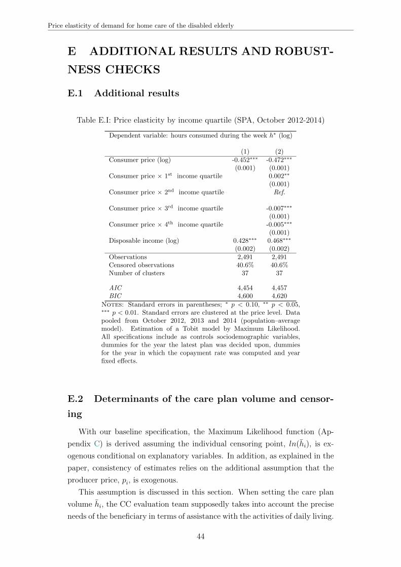
Price elasticity of demand for home care of the disabled elderly
E ADDITIONAL RESULTS AND ROBUST-
NESS CHECKS
E.1 Additional results
Table E.I: Price elasticity by income quartile (SPA, October 2012-2014)
Dependent variable: hours consumed during the week h∗ (log)
(1) (2)Consumer price (log) -0.452∗∗∗ -0.472∗∗∗
(0.001) (0.001)Consumer price × 1st income quartile 0.002∗∗
(0.001)Consumer price × 2nd income quartile Ref.
Consumer price × 3rd income quartile -0.007∗∗∗
(0.001)Consumer price × 4th income quartile -0.005∗∗∗
(0.001)Disposable income (log) 0.428∗∗∗ 0.468∗∗∗
(0.002) (0.002)Observations 2,491 2,491Censored observations 40.6% 40.6%Number of clusters 37 37
AIC 4,454 4,457BIC 4,600 4,620
Notes: Standard errors in parentheses; ∗ p < 0.10, ∗∗ p < 0.05,∗∗∗ p < 0.01. Standard errors are clustered at the price level. Datapooled from October 2012, 2013 and 2014 (population–averagemodel). Estimation of a Tobit model by Maximum Likelihood.All specifications include as controls sociodemographic variables,dummies for the year the latest plan was decided upon, dummiesfor the year in which the copayment rate was computed and yearfixed effects.
E.2 Determinants of the care plan volume and censor-
ing
With our baseline specification, the Maximum Likelihood function (Ap-
pendix C) is derived assuming the individual censoring point, ln(hi), is ex-
ogenous conditional on explanatory variables. In addition, as explained in the
paper, consistency of estimates relies on the additional assumption that the
producer price, pi, is exogenous.
This assumption is discussed in this section. When setting the care plan
volume hi, the CC evaluation team supposedly takes into account the precise
needs of the beneficiary in terms of assistance with the activities of daily living.
44
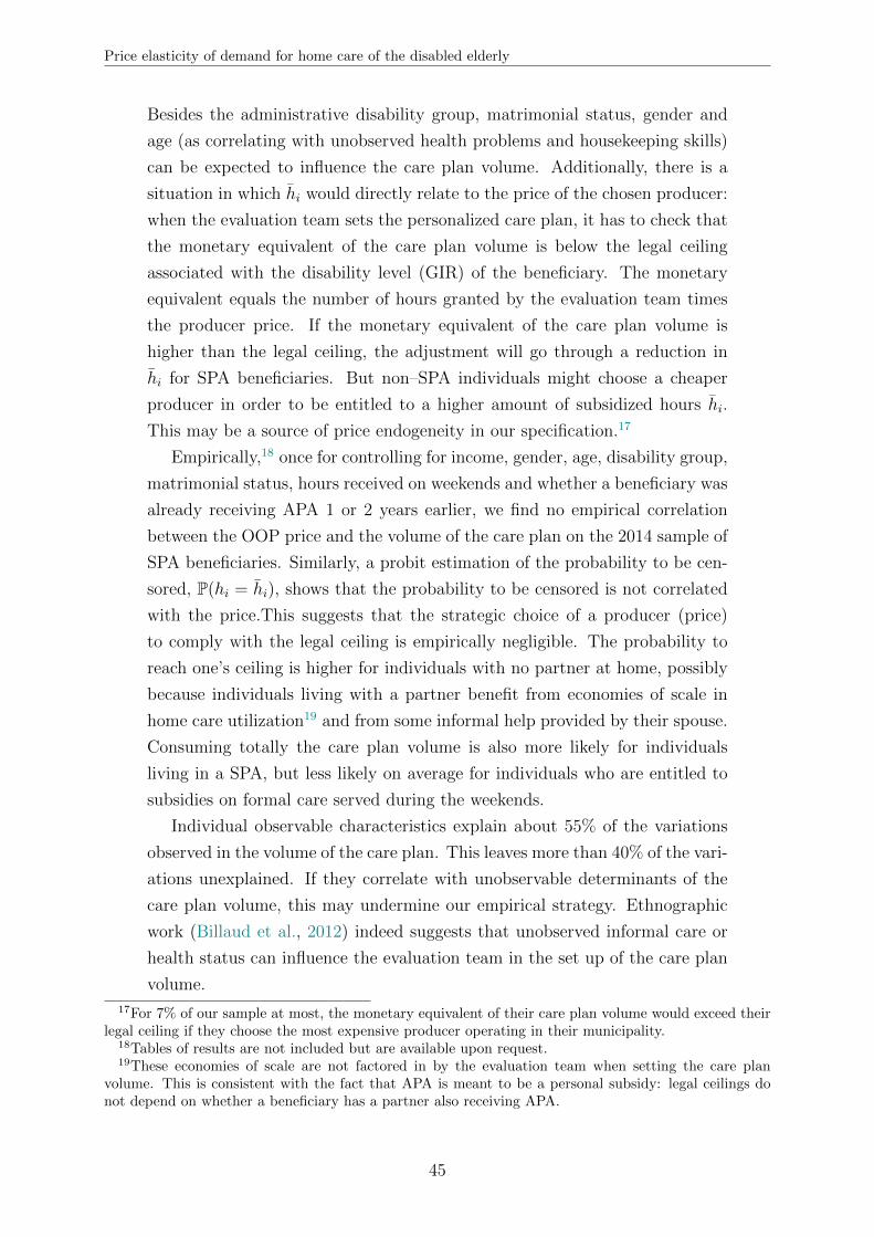
Price elasticity of demand for home care of the disabled elderly
Besides the administrative disability group, matrimonial status, gender and
age (as correlating with unobserved health problems and housekeeping skills)
can be expected to influence the care plan volume. Additionally, there is a
situation in which hi would directly relate to the price of the chosen producer:
when the evaluation team sets the personalized care plan, it has to check that
the monetary equivalent of the care plan volume is below the legal ceiling
associated with the disability level (GIR) of the beneficiary. The monetary
equivalent equals the number of hours granted by the evaluation team times
the producer price. If the monetary equivalent of the care plan volume is
higher than the legal ceiling, the adjustment will go through a reduction in
hi for SPA beneficiaries. But non–SPA individuals might choose a cheaper
producer in order to be entitled to a higher amount of subsidized hours hi.
This may be a source of price endogeneity in our specification.17
Empirically,18 once for controlling for income, gender, age, disability group,
matrimonial status, hours received on weekends and whether a beneficiary was
already receiving APA 1 or 2 years earlier, we find no empirical correlation
between the OOP price and the volume of the care plan on the 2014 sample of
SPA beneficiaries. Similarly, a probit estimation of the probability to be cen-
sored, P(hi = hi), shows that the probability to be censored is not correlated
with the price.This suggests that the strategic choice of a producer (price)
to comply with the legal ceiling is empirically negligible. The probability to
reach one’s ceiling is higher for individuals with no partner at home, possibly
because individuals living with a partner benefit from economies of scale in
home care utilization19 and from some informal help provided by their spouse.
Consuming totally the care plan volume is also more likely for individuals
living in a SPA, but less likely on average for individuals who are entitled to
subsidies on formal care served during the weekends.
Individual observable characteristics explain about 55% of the variations
observed in the volume of the care plan. This leaves more than 40% of the vari-
ations unexplained. If they correlate with unobservable determinants of the
care plan volume, this may undermine our empirical strategy. Ethnographic
work (Billaud et al., 2012) indeed suggests that unobserved informal care or
health status can influence the evaluation team in the set up of the care plan
volume.
17For 7% of our sample at most, the monetary equivalent of their care plan volume would exceed theirlegal ceiling if they choose the most expensive producer operating in their municipality.
18Tables of results are not included but are available upon request.19These economies of scale are not factored in by the evaluation team when setting the care plan
volume. This is consistent with the fact that APA is meant to be a personal subsidy: legal ceilings donot depend on whether a beneficiary has a partner also receiving APA.
45

Price elasticity of demand for home care of the disabled elderly
As we do not have any good instrument to test the endogenity of the
care plan volume in our dataset, we have to rely on the assumption that it
is reasonably exogenous. Still, we can go round the limitations raised by
having an individual–specific censoring point with an alternative specification
we present in the following section. Its second advantage is that it is arguably
more robust to potential price endogeneity.
E.3 Specification in ratio
As presented in Section 4.1 of the paper, our baseline specification is the
following:
ln(h∗i ) = β0 +β1.[ln(pi)+ ln(Iobsi )
]+β2.ln(Iobsi )+
2014∑d=2009
µd.1di + ζ.1e
i +X ′i.θ+ εi
Alternatively, we consider as the dependent variable the share of the care
plan volume that is effectively consumed by the individual, h∗i /hi, that we call
the “relative consumption”. The dependent variable is still censored when
individuals fully consume their care plan volume (exact volume or more), but
the censoring point is unique now.
Empirically, we take the log of the ratio and estimate the following speci-
fication:
ln(h∗ihi
)= α0 + α1.
[ln(pi) + ln(Iobsi )
]+ α2.ln(Iobsi ) + α3.ln(hi)
+2014∑
d=2009
µd.1di + ζ .1e
i +X ′i.θ + εi (11)
The censoring point is thus equal to log(1) = 0 whatever the volume of the
care plan. Equation (11) is equivalent to:
ln(h∗i )− ln(hi) = α0 + α1.[ln(pi) + ln(Iobsi )
]+ α2.ln(Iobsi ) + α3.ln(hi)
+2014∑
d=2009
µd.1di + ζ .1e
i +X ′i.θ + εi
ln(h∗i ) = α0 + α1.[ln(pi) + ln(Iobsi )
]+ α2.ln(Iobsi ) + (α3 + 1).ln(hi)
+2014∑
d=2009
µd.1di + ζ .1e
i +X ′i.θ + εi (12)
In Equation (11), α1 can thus be interpreted as the price elasticity of de-
mand.
46

Price elasticity of demand for home care of the disabled elderly
This specification comes with two advantages. First, it enables us to over-
come the limitation of having an individual–specific censoring point. Specifi-
cation tests that usually come with Tobit models with a fix censoring point
have not been extended to the case of individual–specific censoring. Recent
theoretical developments in semi–parametric estimation methods have pro-
posed ways to deal with individual–varying censoring, but, to our knowledge,
they have not been implemented so far in empirical works.
The specification in ratio additionally permits to address partly the poten-
tial endogeneity of price. In our main results, taking into account the potential
non-random selection into a producer highlights a negative bias of the base-
line estimate. We suspect an omitted variable is negatively correlated with
the price and positively correlated with consumption. Our hypothesis is that
individuals may ex ante choose their producer price according to their individ-
ual “expected level of consumption”. For instance, holding income constant,
beneficiaries with a high expected level of consumption could choose a lower
price to contain their total expenses on home care.
If the consumption of home care h∗i depends on the expected consumption
hexpi , we should estimate the following specification:
ln(h∗i ) = β0+β1.[ln(pi)+ln(Iobsi )
]+β2.ln(Iobsi )+β3.ln(hexpi )
2014∑d=2009
µd.1di +ζ.1ei+X′i.θ+εi
(13)
Schematically, assuming a negative correlation between hexpi and pi (Corrhexpi ,pi <
0 : the more individuals intend to consume, the lower their price) and a pos-
itive effect of hexpi on h∗i (β3 > 0: the higher the expected consumption, the
higher the effective level of consumption), then the omission of hexpi in the
baseline specification can be expected to downward bias coefficient β1.
Using the specification in ratio could partly neutralize this omitted variable
bias in our baseline sample. Indeed, we expect the care plan volume hi to be a
proxy for the expected consumption hexpi . Including hi directly as a control in
our original specification yields interesting results, but raises multi–colinearity
issues, as the care plan volume is highly correlated with the disability level.
Moreover, it does not allow us to go beyond the individual-specific censoring
point problem.
In the following subsections, we present the results obtained with the spec-
ification in ratio using both parametric and semi–parametric regression tech-
niques.
47
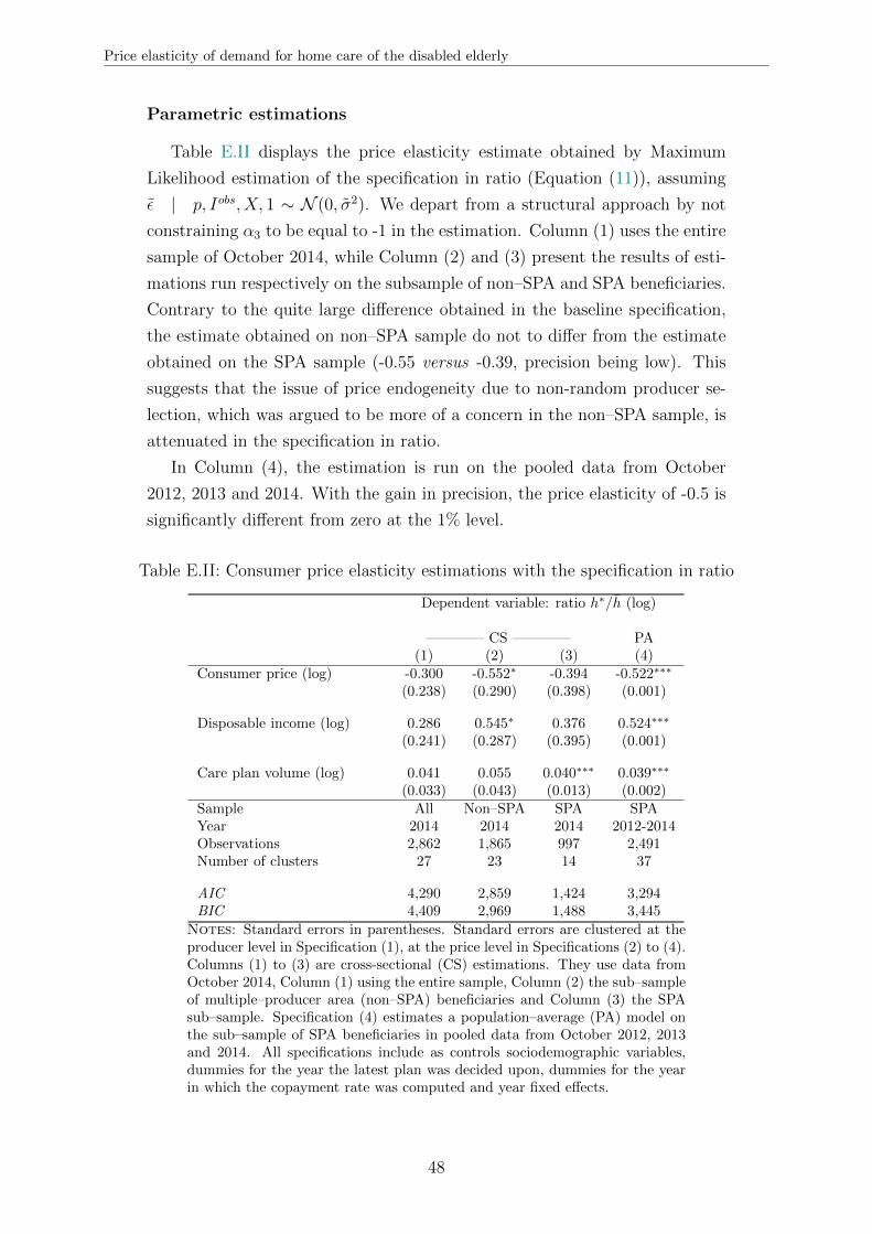
Price elasticity of demand for home care of the disabled elderly
Parametric estimations
Table E.II displays the price elasticity estimate obtained by Maximum
Likelihood estimation of the specification in ratio (Equation (11)), assuming
ε | p, Iobs, X, 1 ∼ N (0, σ2). We depart from a structural approach by not
constraining α3 to be equal to -1 in the estimation. Column (1) uses the entire
sample of October 2014, while Column (2) and (3) present the results of esti-
mations run respectively on the subsample of non–SPA and SPA beneficiaries.
Contrary to the quite large difference obtained in the baseline specification,
the estimate obtained on non–SPA sample do not to differ from the estimate
obtained on the SPA sample (-0.55 versus -0.39, precision being low). This
suggests that the issue of price endogeneity due to non-random producer se-
lection, which was argued to be more of a concern in the non–SPA sample, is
attenuated in the specification in ratio.
In Column (4), the estimation is run on the pooled data from October
2012, 2013 and 2014. With the gain in precision, the price elasticity of -0.5 is
significantly different from zero at the 1% level.
Table E.II: Consumer price elasticity estimations with the specification in ratio
Dependent variable: ratio h∗/h (log)
———— CS ———— PA(1) (2) (3) (4)
Consumer price (log) -0.300 -0.552∗ -0.394 -0.522∗∗∗
(0.238) (0.290) (0.398) (0.001)
Disposable income (log) 0.286 0.545∗ 0.376 0.524∗∗∗
(0.241) (0.287) (0.395) (0.001)
Care plan volume (log) 0.041 0.055 0.040∗∗∗ 0.039∗∗∗
(0.033) (0.043) (0.013) (0.002)Sample All Non–SPA SPA SPAYear 2014 2014 2014 2012-2014Observations 2,862 1,865 997 2,491Number of clusters 27 23 14 37
AIC 4,290 2,859 1,424 3,294BIC 4,409 2,969 1,488 3,445
Notes: Standard errors in parentheses. Standard errors are clustered at theproducer level in Specification (1), at the price level in Specifications (2) to (4).Columns (1) to (3) are cross-sectional (CS) estimations. They use data fromOctober 2014, Column (1) using the entire sample, Column (2) the sub–sampleof multiple–producer area (non–SPA) beneficiaries and Column (3) the SPAsub–sample. Specification (4) estimates a population–average (PA) model onthe sub–sample of SPA beneficiaries in pooled data from October 2012, 2013and 2014. All specifications include as controls sociodemographic variables,dummies for the year the latest plan was decided upon, dummies for the yearin which the copayment rate was computed and year fixed effects.
48
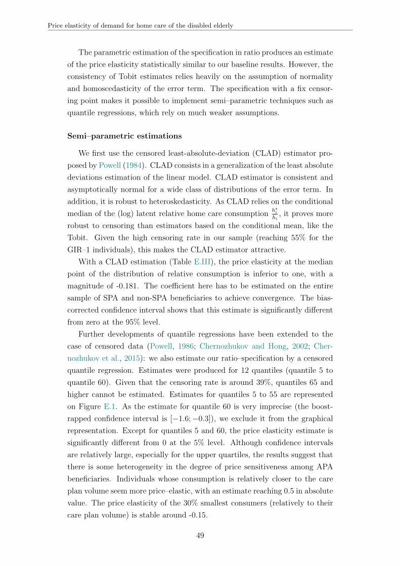
Price elasticity of demand for home care of the disabled elderly
The parametric estimation of the specification in ratio produces an estimate
of the price elasticity statistically similar to our baseline results. However, the
consistency of Tobit estimates relies heavily on the assumption of normality
and homoscedasticity of the error term. The specification with a fix censor-
ing point makes it possible to implement semi–parametric techniques such as
quantile regressions, which rely on much weaker assumptions.
Semi–parametric estimations
We first use the censored least-absolute-deviation (CLAD) estimator pro-
posed by Powell (1984). CLAD consists in a generalization of the least absolute
deviations estimation of the linear model. CLAD estimator is consistent and
asymptotically normal for a wide class of distributions of the error term. In
addition, it is robust to heteroskedasticity. As CLAD relies on the conditional
median of the (log) latent relative home care consumptionh∗i
hi, it proves more
robust to censoring than estimators based on the conditional mean, like the
Tobit. Given the high censoring rate in our sample (reaching 55% for the
GIR–1 individuals), this makes the CLAD estimator attractive.
With a CLAD estimation (Table E.III), the price elasticity at the median
point of the distribution of relative consumption is inferior to one, with a
magnitude of -0.181. The coefficient here has to be estimated on the entire
sample of SPA and non-SPA beneficiaries to achieve convergence. The bias-
corrected confidence interval shows that this estimate is significantly different
from zero at the 95% level.
Further developments of quantile regressions have been extended to the
case of censored data (Powell, 1986; Chernozhukov and Hong, 2002; Cher-
nozhukov et al., 2015): we also estimate our ratio–specification by a censored
quantile regression. Estimates were produced for 12 quantiles (quantile 5 to
quantile 60). Given that the censoring rate is around 39%, quantiles 65 and
higher cannot be estimated. Estimates for quantiles 5 to 55 are represented
on Figure E.1. As the estimate for quantile 60 is very imprecise (the boost-
rapped confidence interval is [−1.6;−0.3]), we exclude it from the graphical
representation. Except for quantiles 5 and 60, the price elasticity estimate is
significantly different from 0 at the 5% level. Although confidence intervals
are relatively large, especially for the upper quartiles, the results suggest that
there is some heterogeneity in the degree of price sensitiveness among APA
beneficiaries. Individuals whose consumption is relatively closer to the care
plan volume seem more price–elastic, with an estimate reaching 0.5 in absolute
value. The price elasticity of the 30% smallest consumers (relatively to their
care plan volume) is stable around -0.15.
49

Price elasticity of demand for home care of the disabled elderly
Table E.III: CLAD estimation of consumer price elasticity (October 2012–2014)
Dependent variable: ratio h∗/h (log)(1)
Consumer price (log)Observed -0.181Bias -0.002Standard error 0.05495% Confidence Interval (BC) [-0.311 ; -0.091]
Replications (Bootstrap) 100Initial sample size 8,190Final sample size 7,502Pseudo R-squared 0.021
Notes: Confidence interval is a bias–corrected (BC) interval.Pooled data from October 2012, 2013 and 2014. Convergencecould not be achieved on the subsample of single–producer areasbeneficiaries. The dependent variable is the log of relative con-sumption. Censored least-absolute-deviation estimation (usingStata user command clad). The specification includes as controlssociodemographic variables, dummies for the year the latest planwas decided upon, dummies for the year in which the copaymentrate was computed and year fixed effects. We were not able toinclude some dummies indicating very rare situations (spouse livingin institution, dummy for the computation of copayment rate in2010): bootstrapped samples picked up unique values for thesevariables.
One word of caution is warranted: as with the CLAD estimation, conver-
gence could not be achieved on the subsample of SPA beneficiaries. Although
we argue that the specification in ratio should decrease the issue of price endo-
geneity, the quantile estimates presented here may still suffer from a potential
upward bias. Our main conclusions though would remain unchanged: quantile
estimates provide further evidence that the price elasticity of the demand for
home care is, on average, substantially inferior to one.
50
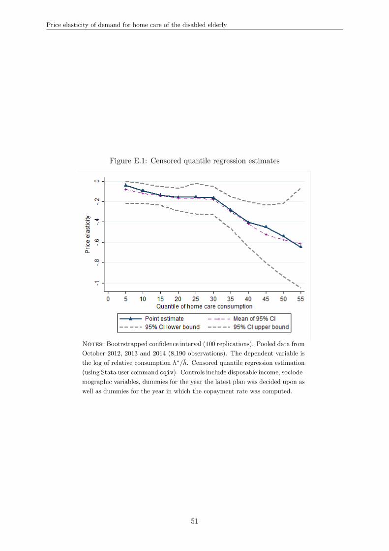
Price elasticity of demand for home care of the disabled elderly
Figure E.1: Censored quantile regression estimates
Notes: Bootrstrapped confidence interval (100 replications). Pooled data from
October 2012, 2013 and 2014 (8,190 observations). The dependent variable is
the log of relative consumption h∗/h. Censored quantile regression estimation
(using Stata user command cqiv). Controls include disposable income, sociode-
mographic variables, dummies for the year the latest plan was decided upon as
well as dummies for the year in which the copayment rate was computed.
51