PC-BASED CONTROL OF HEXAPOD

by

Halil ŞAHBAZ

January, 2007

İZMİR

PC-BASED CONTROL OF HEXAPOD

ABSTRACT

In this study, the aim is to control an hexapod with PC-based control. In this manner, a 6-

DOF parallel manipulator known as hexapod used in the areas such as precise manufacturing

and medicine is examined. For the experimental study, an hexapod is designed and

manufactured. Simulations are done in VisualNASTRAN to determine actuator lengths of the

hexapod. Actuators of the hexapod are linear step motors. In order to control the hexapod, an

integrated VisualBASIC program which uses VisualNASTRAN is developed. The program

runs simulation, takes simulation results as inputs and controls linear step motors via PC-

based motion controllers. Point-to-point open loop control is applied. Positions of the hexapod

in consequence of controlling are measured with a coordinate measuring machine (CMM) and

results are presented. Furthermore, for another experimental study, a servo motor

experimental rig is set with three AC servo motors which are actuators of a 3-DOF serial

manipulator on which the hexapod will be attached. Simulations are done in

VisualNASTRAN to determine actuator positions. VisualBASIC programs whose inputs are

simulation results are developed to control servo motors according to different control

methods and algorithms via PC-based motion control cards. Open loop and closed loop path

tracking control are applied. Results are presented. Motors are successfully followed reference

curves and give good responses regarding proposed algorithms.

Keywords: Hexapod, micro-positioning, PC-based motion control, step motor control, servo

motor control.

HEGZAPODUN BİLGİSAYAR TABANLI KONTROLÜ

ÖZ

Bu çalışmada amaç bilgisayar tabanlı kontrol ile bir hegzapodu kontrol etmektir. Bu

bağlamda, hassas üretim ve tıp gibi alanlarda kullanılan hegzapod olarak bilinen 6 serbestlik

dereceli bir paralel manipülatör incelenmiştir. Deneysel çalışma için, bir hegzapod

tasarlanmış ve imal edilmiştir. Hegzapodun tahrik elemanlarının uzunluklarını belirlemek için

VisualNASTRAN’da simülasyonlar yapılmıştır. Hegzapodun tahrik elemanları adım motor

sürücülü doğrusal motorlardır. Hegzapodun kontrolü için VisualNASTRAN’ı kullanan bir

entegre VisualBASIC programı geliştirilmiştir. Program simülasyonu çalıştırır, simülasyon

sonuçlarını girdi olarak alır ve bilgisayar tabanlı hareket kontrol üniteleri aracılığıyla adım

motor sürücülü doğrusal motorları kontrol eder. Noktadan noktaya açık devre hareket

kontrolü uygulanmıştır. Hegzapodun kontrol sonucundaki konumları, bir koordinat ölçüm

makinesi ile ölçülmüş ve sonuçlar sunulmuştur. Ayrıca, diğer bir deneysel çalışma için

üzerine hegzapodun bağlanacağı bir 3 serbestlik dereceli seri manipülatörün tahrik elemanları

olan üç AC servo motor ile, bir servo motor deney düzeneği kurulmuştur. Tahrik

elemanlarının konumlarını belirlemek için VisualNASTRAN’da simülasyonlar yapılmıştır.

Servo motorların değişik kontrol yöntemleri ve algoritmalara göre bilgisayar tabanlı hareket

kontrol kartları üzerinden kontrolü için, girdileri simülasyon sonuçları olan VisualBASIC

programları geliştirilmiştir. Açık devre ve kapalı devre yörünge izleme kontrolü

uygulanmıştır. Sonuçlar sunulmuştur. Motorlar önerilen algoritmalara göre hedef eğrileri

başarıyla takip etmiş ve iyi cevaplar vermişlerdir.

Anahtar sözcükler: Hegzapod, mikro-konumlandırma, bilgisayar tabanlı hareket kontrolü,

adım motor kontrolü, servo motor kontrolü.

1. Introduction

Controlling of robot manipulators in micron ranges is an important issue of developing

technology. Micro-positioning robots have a wide variety of applications from surgery robots

to space shuttles. These robots can precisely follow a path described with respect to the work.

Working with more precise motions and making more precise machines decrease errors which

might come into existence because of effects of standard machines and workers. By more

precise manufacturing machines, dimensions of manufactured parts become more accurate.

Machines which made by more accurate parts work with less errors. Thus, machines make

much more accurate and reliable products. Parallel manipulators are used for micro-

positioning. Best-known type of parallel manipulators is hexapod. Hexapods are suitable for

micro-positioning, because hexapods have 6 degrees of freedom.

In this study, PC-based control of a 6-DOF parallel manipulator namely hexapod is

comprised. In this manner, hexapod for micro-positioning and controlling of actuators of a

serial manipulator on which the parallel manipulator will be attached at future works are

considered. Actuators of the hexapod and the serial manipulator are linear step motors and

brushless AC servo motors, respectively. These actuators are controlled by PC-based motion

control cards. Point-to-point open loop control is applied to linear step motors, so to hexapod;

and open loop and closed loop control is applied to servo motors for path following.

6-DOF parallel manipulators were firstly used by Gough & Whitehall (1962) as a tire-

testing machine. The testing machine was consisted of a six-linear jack system. Stewart

(1965) designed a 6-DOF parallel manipulator for the usage of flight simulator. A systematic

study of kinematic structures of parallel manipulators was made by Hunt (1983). Since then,

parallel manipulators have been taking interests of researchers. Wendlandt & Sastry (1994)

examined a Stewart platform for endoscopy in order to design and control. The researchers

aimed the platform to follow a circled path. McInroy (1999) investigated controlling of

hexapods by dynamic modelling. Base accelerations were included and the model was

experimentally verified. A comprehensive literature review study was made by Dasgupta &

Mruthyunjaya (2000). The study contained all topics about hexapods and researches related to

these topics made until the publication year. An important study about parallel manipulators

was the investigating new kinematic structures for parallel manipulators (Gao, Li, Zhao, Jin &

Zhao, 2002). In that study, researchers developed new types of composite links. Joint types

related to degree of freedom were presented. Alizade & Bayram (2004) classified parallel

manipulators according to their platform types and connections between them. In another

study, active vibration control of an hexapod was achieved with sensitivity weightened linear

quadratic Gaussian (SWLQG) controller (Hauge & Campbell, 2004). Inverse kinematics,

forward kinematics, error analysis and workspace evaluation were examined in the paper of

Jelenkovic, Jakobovic & Budin (2004). Drive singularities of parallel manipulators were

investigated by Ider (2005). Kim, Cho & Lee successfully controlled a 6-DOF parallel

manipulator, namely hexapod, with respect to robust nonlinear control. The researchers

considered friction of each actuator because friction may degrade control performance. In this

manner, in order to determine friction values, a friction estimator was used. Karagülle, H.,

Sarıgül, S., Kıral, Z., Varol, K., & Malgaca, L. (01 July 2006, 01 July 2007) have published

reports about micro-positioning robots.

There are many researches about controlling of servo motors and step motors. Van de

Straete, Degezelle, De Schutter & Belmans (1998) have investigated servo motor selection

criterions for mechatronic applications. Servo motors were modelled and simulated by using

their mechanical and electrical properties in the paper of Dulger, Kirecci, & Topalbekiroglu

(2001). By fuzzy logic control, an ultrasonic motor (Bal, Bekiroglu, Demirbas, & Colak,

2004) and a DC servo motor (Khongkoom, Kanchanathep, Nopnakeepong, Tamthong,

Tunyasrirut, & Kagawa, 2000), (Lin, 1994) and (Lu, 1997) were controlled. Dandil,

Gokbulut, & Ata (2004) and Lin & Wai (1998) investigated, respectively, asynchronous

motors and synchronous motors with hybrid controllers which were adjusted by proportional-

integral (PI) controllers via neural networks. Servo motors were controlled by various type

control methods such as H∞ robust control (Ximei & Qingding, 2005), adaptive fuzzy sliding-

mode (Lin & Chiu, 1998), variable structure approach (Hashimoto, Yamamoto, Yanagisawa,

& Harashima, 1988), micro-processor based robust control (Tzou & Wu, 1990) and learning

approach (Han, Kim, Ha, Lee, & Park, 1995). Lin, Jan, Hwang, & Tsai (2003) studied

kinematic analyses of hexapods and controlling of AC servo motors which were used as

actuators of hexapods in their study. Controlling of AC servo motors were achieved by using

an estimator which estimated the rotor position as feedback (Yoneya, Yoshimaru, & Togari,

2000). Comparison of different servo motor drivers can be found in the study of Yamamoto &

Shinohara (1996). Grimbleby (1995) and Crnosija, Adjukovic, & Kuzmanovic (1999) made

studies on closed loop control algorithms of step motors and controlled step motors by using

these algorithms. Mort, Abbod, & Linkens (1995) compared step motors which controlled by

open loop control with proportional-integral (PI) controllers, and DC servo motors which

controlled by closed loop fuzzy logic control. These two types of motors and methods gave

good responses. Studies about PC-based control systems are as followings: Path tracking of a

3-DOF CNC machine with circular and linear interpolation was examined; and tracking error

was desired to decrease to minimum (Yang, & Hong, 2001). Ku, Larsen, & Cetinkunt (1998)

used PC-based motion control cards for nano-positioning diamond machining tools. They also

controlled the system by neural network. Noorani (1990) dealt with controlling of a 6-DOF

robot manipulator actuated by step motors by giving position and orientation inputs via a

computer. Şahbaz (2007) have studied PC-based control of an hexapod and 3-DOF serial

manipulator via motion control cards.

2. Initial Design of the Hexapod

There are a lot of different structures of hexapods. After reviewing the literature, some

different structures were created manually in VisualNASTRAN (MSC Software Corp., 2006),

to examine which type is optimal with respect to joint positions. In this section, different joint

positions are tried and kinematic and kinetic analyses are performed in VisualNASTRAN.

2.1 Initial Design

In order to test different joint positions and to find characteristics of actuators and joints, a

basic model is created (Karagülle et al., 2006). The basic model consists of a movable upper

platform, a fixed lower platform and linear actuators.

2.2 Kinematic Analysis

A VisualBASIC program is developed to create “prescribed motion”. Vx, Vy, Vz, Wx, Wy,

and Wz values are assigned as prescribed motion. These are created with the VisualBASIC

program with respect to a velocity sinusoid (Karagülle et al., 2006). It is desired the upper

platform to move (0, 0, 0.23; 0, 0, 0) world coordinate point to (0, 0.03, 0.2; 10, 0, 0) world

coordinate point in 3 seconds. 0.6 seconds is acceleration time and 0.6 seconds is deceleration

time and 1.8 seconds is constant velocity motion time (Karagülle et al., 2006). Meters are

assigned to linear actuators to measure actuator lengths. Meters give lengths of actuators

while the program is running. Data of meters can be taken by a VisualBASIC program. By

comparing the values, maximum actuator length change is found as 47.58 mm.

2.3 Kinetic Analysis

Actuator lengths are assigned with values which have been found by kinematic analysis. Fx

= -10 N, Fy = -10 N, Fz = -100 N force inputs, and Tx = 1 Nm, Ty = -1 Nm, Tz = 0 Nm torque

inputs are applied to the centre of the upper platform. Duration of the motion is taken 3 s and

number of samples is 21 likewise the kinematic analysis. Constraint tension meters are

created on the linear actuator constraints to measure actuator forces. Meters read the forces

which occurred when the motion progresses. After the motion is stopped, maximum actuator

force is found as 54.563 N with a subroutine of the VisualBASIC project which is developed

(Karagülle et al., 2006).

3. Selection of Appropriate Actuators and Joints

Choosing appropriate actuators and joints is an important part of creating an hexapod;

because, active parts of an hexapod are linear motors and joints. Other parts are rigidly

connected. In this section, choosing procedure of actuators and joints is presented.

3.1 Selecting Appropriate Linear Actuators

Linear motors and joints were searched over the world and correspondences were made

with companies which have web sites. Products were compared in terms of minimum stroke

and minimum force requirements found from kinematic and kinetic analyses of the initial

design. They were also compared in terms of containing feedback devices, dimensions,

precisions, velocities, weights, costs and delivery times. After the comparing process, 4000

pulses/rev precision encoders attached 43K4U – 05 – 032ENG type linear motors of HSI

Company (HSI Co., 2006) are supplied.

3.2 Selecting Appropriate Joints

As a result of comparing spherical joints which are determined by searching the joint

suppliers all over the world, twelve items of SRJ008C type 2.5 μm precision spherical joints

of Hephaist Company (Hephaist Co., 2006) are supplied.

4. Design and Manufacturing of the Hexapod

Parts of the hexapod except from standard parts such as actuators and spherical joints are

designed and manufactured. In this section, design and manufacturing of parts of the hexapod

are presented. Control and driver systems of the hexapod are also set; and these systems are

carried out.

4.1 Design of the Hexapod

Parts of the hexapod except from standard parts such as linear actuators and spherical

joints are designed. Linear motor and spherical joint dimensions are taken as the base for

design. Design of the parts is done with I-Deas solid modelling program. Modifications of the

parts are made with SolidWorks (SolidWorks Corp., 2006) solid modelling program, if

needed. Solid models of standard parts are also created for simulation (Karagülle et al., 2007).

3D solid models of all parts including linear motors and spherical joints are imported

manually into VisualNASTRAN to test joint locations on the upper and lower platforms. The

model is constructed manually in the program. Joint locations on the upper platform are not

changed. However, joint locations on the lower platform are changed until the parts are not

collided in the simulation when the hexapod goes to its limit points. The angle between

closest joint locations on the lower platform is designated. In order to test colliding; φb is

changed 20 deg to 30 deg. Hexapod is moved to end points and parts are observed. It is

observed that no risk is occurred when φb = 30 deg. Therefore, the angle between closest

joints on lower platform (φb) is decided as 30 deg. Details of the platforms are determined,

the parts are designed and 3D models of the parts are created.

4.2 Manufacturing of the Hexapod

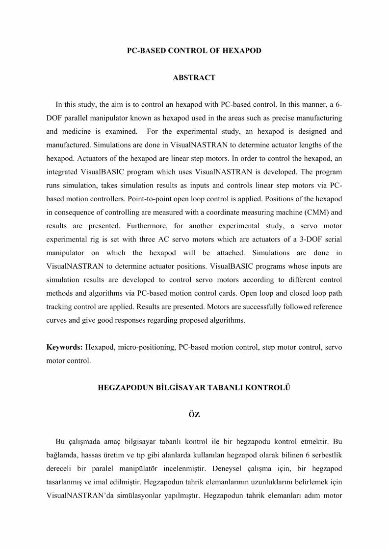
Hexapod consists of a lower platform, joints, lower connection parts, linear motors, upper

connection parts, stud bolts, joint connection parts and an upper platform. After generating 2D

manufacturing drawings, parts are manufactured. All parts are made from stainless steel

(AISI304, 1.4401 standards) (Karagülle et al., 2007). A simulation view and a view of the

manufactured hexapod are shown in Figure 1.

Figure 1. Views of the simulation and the manufactured hexapod.

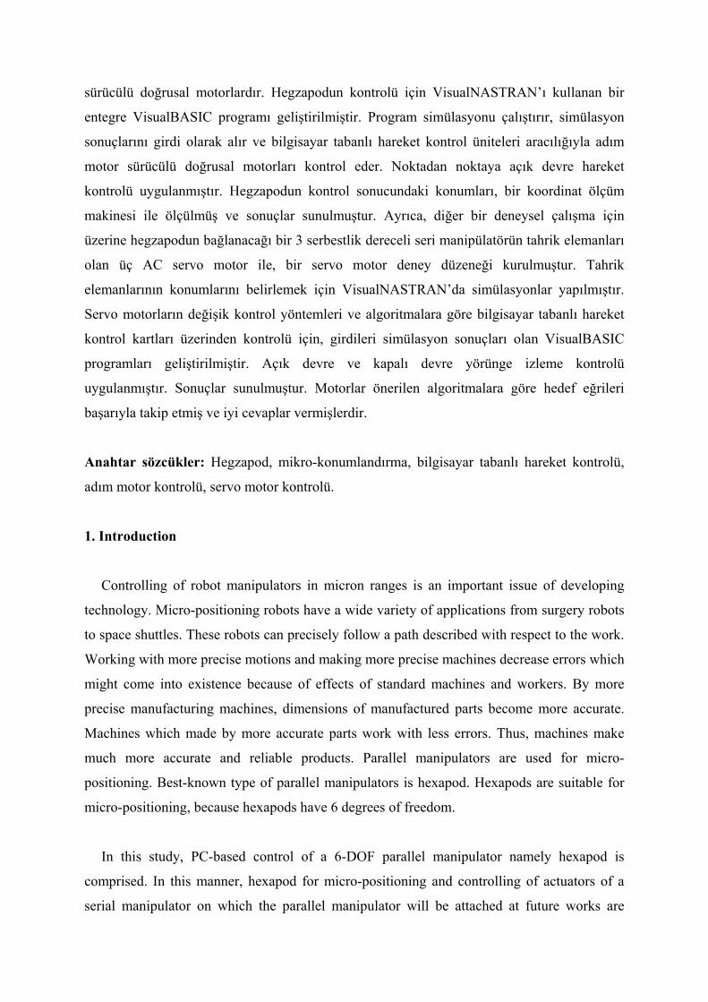
4.3 Hexapod Control System

The hexapod control system consists of linear motor drivers, PCI motion control cards and

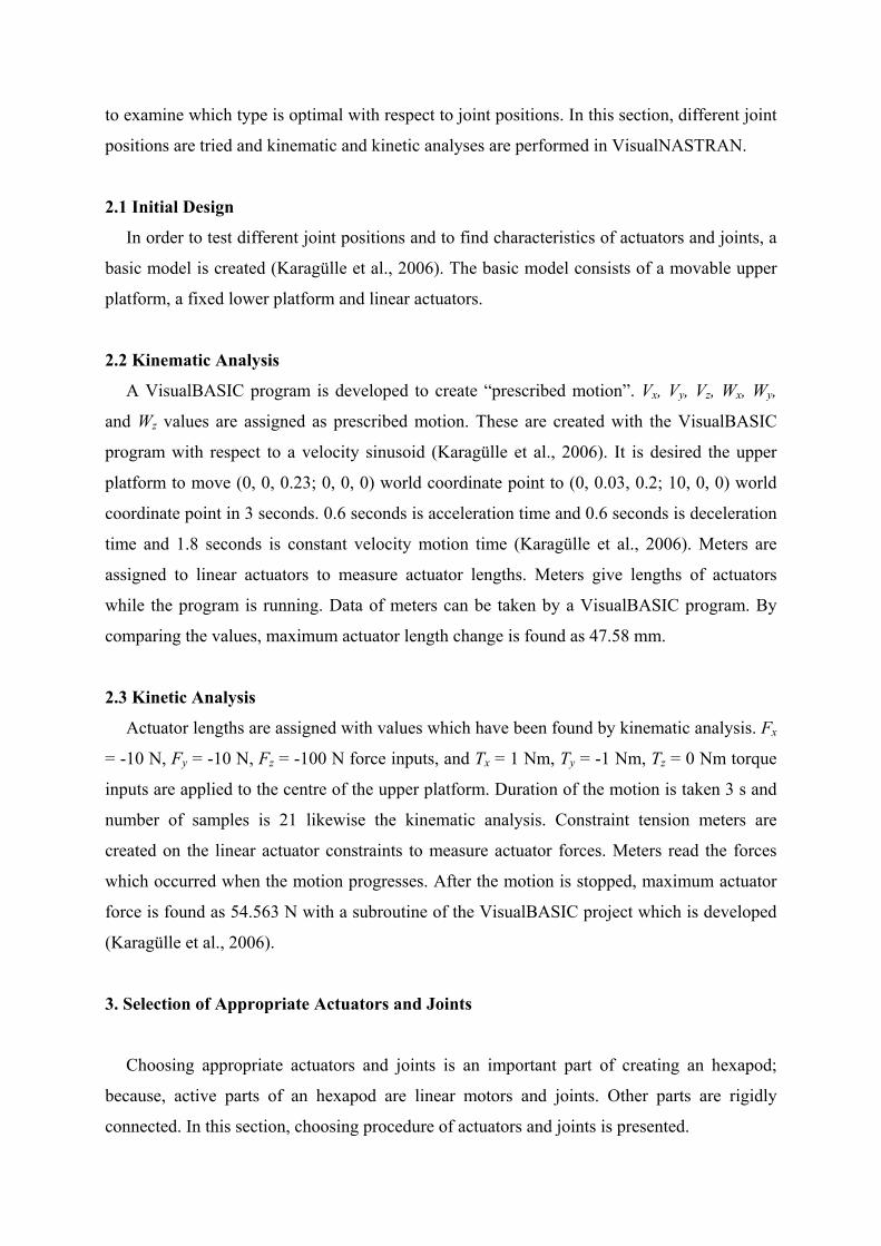
a power supply. A schematic view of the system is shown in Figure 2. The control system is

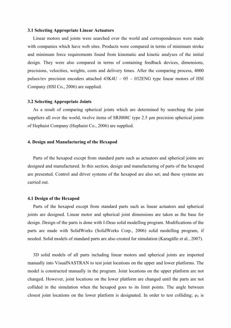
also shown in Figure 3. A portable control panel is designed and manufactured for the control

system. A detailed view of the control panel is in Figure 4. The control panel comprises a

power supply, a distributor of the power supply, ADLINK PCI 8132 and PCI 8164 (Adlink

Technology Inc., 2006) motion control cards, linear motor drivers and cables. In the control

panel and hexapod control system, PCI 8132 card is connected to 1st and 2nd drivers, PCI 8164

card is connected to 3rd, 4th, 5th and 6th drivers. Drivers and control cards need 24VDC power

for operation. This power is supplied from the 24VDC power supply and allocated by the

manufactured distributor of the power supply.

The control panel is designed. Connections between controllers and drivers; and controllers

and encoders are made. The hexapod is electronically prepared for motion tests.

PCI 8132 PCI 8164

24VDC Power supply

Distributor of power supply

1. driver 2. driver 3. driver 4. driver 5. driver 6. driver

Figure 2. A schematic view of the control system.

1. motor 2. motor 3. motor 4. motor 5. motor 6. motor

Figure 3. A view of the control system.

Figure 4. A detailed view of the control panel.

5. Simulation and Controlling of th

ntrol the hexapod. Simulation is performed

by VisualNASTRAN. Simulation gives values of inverse kinematic solution as outputs.

PC

Control

CMM

panel Hexapod

Linear motor

e Hexapod

In this section, it is desired to simulate and co

Drivers (1, 2)

PCI 8132

24VDC power supply

Manufactured distributor of power supply

PCI 8164

Bus cables

Drivers (3, 4, 5, 6)

SJ pin cables

Co

pod

isualNASTRAN has API (Application Programming Interface) property. Therefore, it

ming VisualNASTRAN, design and inputs

can

STRAN model is constructed with simple 3D models according to real

hexapod, in order to have a rapid process. Detailed 3D models might be slowed the programs.

Th

ntrolling of the hexapod is achieved by a developed VisualBASIC program. This program

manages VisualNASTRAN and takes outputs of VisualNASTRAN as inputs (Karagülle et al.,

2007). For the designed hexapod (Fig. 1), dimensions of the fixed lower platform: diameter is

348 mm, thickness is 11 mm and the angle between closest joints is 30 deg. The centres of

spherical joints are on a circle whose diameter is 298 mm and 6 mm above from the upper

surface of the fixed lower platform. Dimensions of the movable upper platform: diameter is

250 mm, thickness is 10 mm and the angle between closest joints is 60 deg. The centres of

spherical joints are on a circle whose diameter is 200 mm and 6 mm below from the lower

surface of the movable upper platform. Distance in the z direction between the upper surface

of the lower platform and the lower surface of the upper platform is 233.1362 mm when the

actuators, consequently the hexapod, are fully closed. Stroke of the linear motors is 50.8 mm

and maximum tilt angle of the joints is 45 deg. Global z axis is perpendicular to the line which

ties centres of the 1st spherical joint and the 6th spherical joint. Global x-y plane is parallel to

the surface of the lower platform. Direction of the global z axis is along a line which goes to

the upper platform from the lower platform.

5.1 Simulation and Controlling of the Hexa

V

can be programmed by VisualBASIC. By program

be parametrical. Any changes are possible by changing the parameters. Application can

be easy and rapid. Simulation and controlling of hexapod are achieved by a VisualBASIC

program. This program assembles solid parts, simulates the hexapod and solves inverse

kinematic analyses and controls linear motors as point-to-point application via PCI motion

control cards.

A VisualNA

ere are an upper moving platform, a fixed lower platform, a rectangular part which

represents constant part of a link and a cylindrical part which represents moving part of a link

in the basic kinematic model. These parts are in dimensions of designed hexapod. This model

can be seen in Figure 5 (Karagülle et al., 2007). Input values of the simulation are xp, yp, zp,

θxp, θyp and θzp. xp, yp and zp are desired positions of the movable upper platform in mm along

x, y and z directions, respectively. When all linear motors are fully retracted, xp = 0, yp = 0 and

zp = 0. Assume that, movable axis system which is in the centre of upper platform is x1, y1 and

z1. Desired rotation about x1 is θxp; desired rotation about y1 is θyp and then desired rotation

about z1 is θzp. Angles are in degrees. When all linear motors are fully retracted, θxp = 0, θyp =

0 and θzp = 0.

Figure 5. Basic model of the hexapod.

Open loop position c linear motors. Point – to – point

applications are processed. PC-based motion control is achieved over PCI 8132 and PCI 8164

mo

velocities are determined by using

interpolation. The maximum velocity is chosen as 3000 pulse/s. The biggest distance

ex

ved by simulation results after determining

command parameters of motion control cards with respect to position and velocity data. T

Z

Y

X

ontrol is applied to hexapod via

tion control cards. Control of hexapod manipulator is based on inverse kinematics

(Jelenkovic et al., 2004). The simulation (inverse kinematic solution) gives length changes of

linear motors with respect to time. These values are taken as inputs. If the “Move” command

button is clicked on the developed VisualBASIC program interface, pulse numbers which will

be applied to linear motors are determined with respect to the difference between initial

position and final position of the moving upper platform.

In order to start and stop movement simultaneously,

tracted (or retracted) linear motor has the biggest velocity (3000 pulse/s). The slowest linear

motor with respect to the motion moves the less.

Hexapod which has been manufactured is mo

ve

os, svel, mvel, tacc, tdec) (1)

l is s

velocity (pulse/s), mvel is maximum velocity (pulse/s), tacc is acceleration time (s) and tdec is

de

are calculated according to lengths

of axes (linear motors), as follows:

locity profile command is used fundamentally in the program. The commands are as

following formulas (1) and (2):

B_8164.StartTAMove(axis, p

B_8132.StartTMove(axis, pos, svel, mvel, tacc, tdec) (2)

Where, axis is the working axis number, pos is position input (pulse), sve tarting

celeration time (s). For the applications, they are taken that svel = 0 and tacc = tdec = 0.01

s. mvel is determined as 3000 pulse/s for the axis which has maximum length change. mvel for

other axes is calculated by interpolation explained above.

Pulse numbers are position information. Pulse numbers

00075.0idis

pos = , i = 1, 2, …, 6 i (3)

Where, dis is length changes, which is found by inverse kinematic solution, of the linear

motors, pos is numbers of pulses. If 1 pulse is sent, then linear motors move 0.75 μm; because

ste

the hexapod whose manufacturing is discussed in Section 4

re presented. Tests are made by the developed VisualBASIC program which is explained in

Se

p motors are bipolar. Precision of motors is 1.5 μm, 2 pulses give this value regarding

bipolar type. Consequently, commands (1) and (2) are sent linear motors as point – to – point

open loop control via motion control cards.

6. Test Results of the Hexapod

In this section, test results of

a

ction 5. Test results occurred from desired position (xp, yp, zp) and orientation (θxp, θyp, θzp),

which are explained in Section 5, of the movable upper platform are measured by a coordinate

measuring machine (CMM). Model of the CMM is Euro-C-A9106 of Mitutoyo Company

(Mitutoyo Corp., 2006). Precision of the CMM is 5 μm.

6.1 Tests and Results

Positions of the upper platform are measured by CMM. In order to test, global axis system

f the CMM is translated to global axis system of the hexapod. xp and yp is measured by

nt using lateral faces of the upper platform. zp, αp, βp and γp is

de

he upper platform is

moved 14 times to different positions and then returned to the initial position. Average values

(xp

xp, yp, zp αp, βp, γp

εx, εy, εzεα, εβ, εγ

ges, respectively 2, 3

o

creating a circle eleme

termined by measuring the plane of upper surface of the upper platform. αp, βp and γp are

angles between x, y and z axes and z1 axis which is attached to upper platform, respectively.

αp, βp and γp can be generated from θxp, θyp and θzp with a transformation.

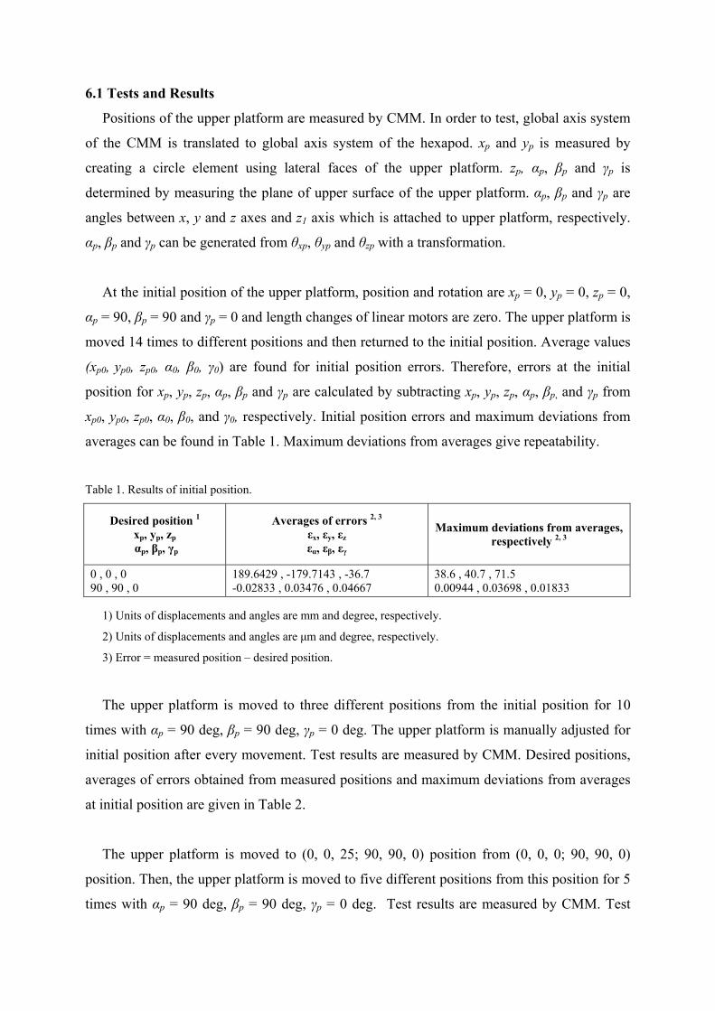
At the initial position of the upper platform, position and rotation are xp = 0, yp = 0, zp = 0,

αp = 90, βp = 90 and γp = 0 and length changes of linear motors are zero. T

0, yp0, zp0, α0, β0, γ0) are found for initial position errors. Therefore, errors at the initial

position for xp, yp, zp, αp, βp and γp are calculated by subtracting xp, yp, zp, αp, βp, and γp from

xp0, yp0, zp0, α0, β0, and γ0, respectively. Initial position errors and maximum deviations from

averages can be found in Table 1. Maximum deviations from averages give repeatability.

Table 1. Results of initial position.

Desired position Averages of errors Maximum deviations from avera1 2, 3

0 , 0 , 0 189.6490 ,

29 , -179.7143 , -36.7 -0.0283

38.6 , 40.7 , 71.5 0.00944 , 0.03698 , 0.01833 90 , 0 3 , 0.03476 , 0.04667

1) Un ents and angles are m egree, respectively.

2) Units of displacements and angles are μm and degree, respectively.

= measured positi

from the initial position for 10

tim deg. The upper platform is manually adjusted for

initial position after every movement. Test results are measured by CMM. Desired positions,

av

oved to five different positions from this position for 5

mes with αp = 90 deg, βp = 90 deg, γp = 0 deg. Test results are measured by CMM. Test

its of isp d lacem m a d dn

3) Error on – desired position.

The upper platform is moved to three different positions

es with αp = 90 deg, βp = 90 deg, γp = 0

erages of errors obtained from measured positions and maximum deviations from averages

at initial position are given in Table 2.

The upper platform is moved to (0, 0, 25; 90, 90, 0) position from (0, 0, 0; 90, 90, 0)

position. Then, the upper platform is m

ti

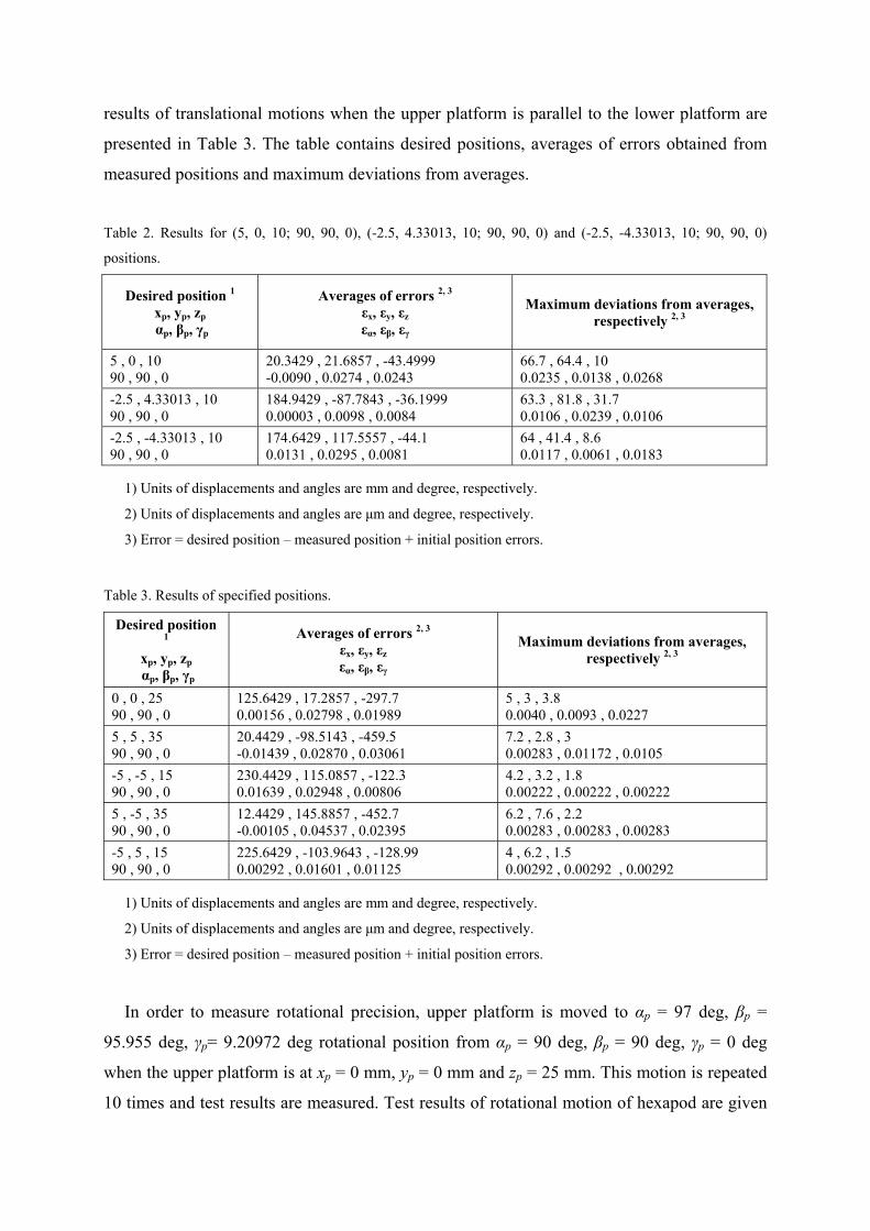
res

Desired position 1 Averages of errors 2, 3Maximum deviations from averages,

ults of translational motions when the upper platform is parallel to the lower platform are

presented in Table 3. The table contains desired positions, averages of errors obtained from

measured positions and maximum deviations from averages.

Table 2. Results for (5, 0, 10; 90, 90, 0), (-2.5, 4.33013, 10; 90, 90, 0) and (-2.5, -4.33013, 10; 90, 90, 0)

positions.

xp, yp, zp αp, βp, γp

εx, εy, εzεα, εβ, εγ

respectively 2, 3

5 , 0 , 10 90

20.3429 , 21.6857 , -43.4999 -0.0090

66.7 , 64.4 , 10 0.0235 , 0.0138 , 0.0268 , 90 , 0 , 0.0274 , 0.0243

-2.5 , 90 , 90

184.9429 9 0.00003 , 0.009 4

60.0106 , 0.0

4 0 .33013 , 1 , 0

, -87.7 199843 , -36.8 , 0.008

3.3 , 81.8 , 31.7 239 , 0.0106

-2.5 , -4.33013 , 10 174.6429 , 117.5557 , -44.1 64 , 41.4 , 8.6 90 , 90 , 0 0.0131 , 0.0295 , 0.0081 0.0117 , 0.0061 , 0.0183

1) Units of displacemen , respectiv

of displacemen gree, respective

sit n er

Tab

D

xp, yp, zpεx, εy, εzεα, εβ, εγ

mum deviations from averages, respectively 2, 3

ts and angles are mm and degree ely.

2) Units ts and angles are μm and de ly.

3) Error = desired po ion – measured position + initial positio rors.

le 3. Results of specified positions.

esired position 1

αp, βp, γp

Averages of errors 2, 3Maxi

0 , 0 , 25 125.6429 , 17.2890 , 90 , 0

57 , -297.7 0.00156 ,

5 , 3 , 3.8 0.0040 , 0.0093 , 0.0227 0.02798 , 0.01989

5 , 5 , 3590 ,

20.4429 , -9-0.01439 , 0.0287 61

7.0.00283 , 0.0

90 , 0

8.514 3 , -459.50 , 0.030

2 , 2.8 , 3 1172 , 0.0105

-5 ,

230.4429 , 115.0857 , -122.3 4.2 , 3.2 , 1.8 .00222 , 0.00222

-5 , 15 90 , 90 , 0 0.01639 , 0.02948 , 0.00806 0.00222 , 05 , -5 , 35 90 , 90 , 0

12.4429 , 145.8857 , -452.7 -0.00105 , 0.04537 , 0.02395

6.2 , 7.6 , 2.2 0.00283 , 0.00283 , 0.00283

-5 , 5 , 15 90 , 90 , 0

225.6429 , -103.9643 , -128.99 292 , 0.00292 0.00292 , 0.01601 , 0.01125

4 , 6.2 , 1.5 0.00292 , 0.00

1) Units of displac d degree, respec

of displac degree, respect

desired itial position

is moved to αp = 97 deg, βp =

95 deg, βp = 90 deg, γp = 0 deg

when the upper platform is at xp = 0 mm, yp = 0 mm and zp = 25 mm. This motion is repeated

10 times and test results are measured. Test results of rotational motion of hexapod are given

ements and angles are mm an tively.

2) Units ements and angles are μm and ively.

3) Error = position – measured position + in errors.

In order to measure rotational precision, upper platform

.955 deg, γp= 9.20972 deg rotational position from αp = 90

in

respectively 1, 2

Table 4. The table has the desired position; averages of errors calculated from measured

angular positions and maximum deviations from averages.

Table 4. Results of rotational motion.

Desired position 1 αp, βp, γp

Averages of errors 1 ,2

εα, εβ, εγMaximum deviations from averages,

97 , 95.955 , 9.20972 -0.3239 , 0.1108 , -0.1326 0.004 , 0.004 , 0.014

1) Units of angles are degree.

2) Error = desired position – test osition err

re a rs (Table 1) otors are fully

closed. Tab isions and repeatability, because motions are

sta otors are manually closed by

using the program. Therefore, deviations are high in these motions. Limit switches attached to

lin

s namely maximum deviations are about desired values. However,

measured positions and desired positions are different. This difference can not be considered

for

sembly errors. Simulations contain no

ma ufacturing and assembly errors. Precision can be increased by simulating the system with

ini

result position + initial p ors.

As a result, the re initial position erro when all linear m

le 2 may give an idea about prec

rted from the initial point. However, in those tests linear m

ear motors can be used to fully close the linear motors instead of manual closing. Thus, the

upper platform of the hexapod can be set in the same point at the initial position. Therefore,

precision and repeatability regarding the motions which are started from the initial position

can be improved.

Five different points (Table 3) are also tested. Hexapod is moved to every point in a

sequence. In addition, rotational motion (Table 4) is tested. Consequence of these tests,

repeatability value

motions in a sequence, because errors of previous motion effect actual motion, and errors

of actual motion effect following motion. Maximum deviations are important in these

motions. It is observed that, the hexapod moves to approximately same positions. This means,

hexapod can move right positions after calibrating it.

As results of measurements, it is observed that precision of the hexapod is worse than

repeatability. This difference can be caused by initial position errors, and initial position

errors can be caused by manufacturing errors and as

n

tial position errors or making more precise manufacturing and assembly.

7. Controlling of AC Servo Motor Systems

Motors can be controlled by PC-based units or programmable stand-alone units in

utomation systems. In this section, controlling of servo motors is carried out by ADLINK

al study, an experimental rig is constructed and

VisualBASIC programs are developed to control simultaneously three OMRON brushless AC

ser

achieved by VisualNASTRAN. Starting

and final positions of the end point is determined. Between these points, linear motion is

city sinusoid.

Ge

Figure 6. The designed 3-DOF serial manipulator.

a

PCI motion control cards. For the experiment

vo motors (Omron Corp., 2006) over the cards. In the programs, reference velocity and

position curves are taken as inputs, and the parameters of the commands of ADLINK control

cards are determined. In this study, servo motors are thought as actuators of a 3-DOF serial

manipulator on which the hexapod will be attached.

7.1 Design and Inverse Kinematic Analyses of a 3-DOF Serial Manipulator

Solid models of parts of a 3-DOF manipulator are created parametrically in ABAQUS

(Abaqus Inc., 2006). Inverse kinematic analyses are

supposed. Velocity inputs of the end point are generated with respect to velo

nerated velocity values are applied to end point. Inverse kinematic analysis is solved by

VisualNASTRAN. Results of the solution are angular velocities and angular positions of the

actuator. These curves are inputs of control algorithms (Karagülle et al., 2006). The 3-DOF

serial manipulator can be seen in Figure 6.

p2

p3a

p3b

p0

p1 End point

7.2 AC Servo Motor Experimental Rig

AC servo motors are thought as actuators of a 3-DOF serial manipulator. The experimental

rig set up with Omron brushless AC servo motors, are shown in Figure 7, schematically.

Figure 7. Servo motor experimental rig.

tems

brushless AC servo motors and their servo drivers of Omron Company are used in the

experimental rig. The experimental rig which is set up at laboratory is given in Figure 8.

Encoders are serially attached to motors. Servo motor drivers have one motor driving

capacity. 203123 type Maxon planetary gears (Maxon Co., 2006) whose reduction ratio is 74

are assembled to servo motors. Flanges and pinion gears are designed and manufactured in

order to assemble motors and gears.

PCI 8132 and PCI 8164 motion control cards of Adlink Company and three i

Figure 8. The experimental rig.

PC

Connectors

Power supply distributor connecto

Power supply

Terminals r

Servo motor drivers

Servo motors

7.3 Controlling of AC Servo Motors

Position input of the cards must be pulse numbers and velocity input of the cards must be

pulse numbers per a second; however, for comprehensibility, position is taken in meters (or

degrees) and velocity is taken in revolution per minute in the developed programs. Position

and velocity values of motors are 2048 pulse/rev and 2048 pulse/s, respectively. These inputs

are calculated as following:

pdngearp .3602048

= (4)

pmngearr

p ..2

2048

0π= (5)

vdngearv .60

= 2048 (6)

dius of shaft or pulley etc. attached to the shaft of gear.

Closed loop control of two servo motors is tested by a developed VisualBASIC program

This program is given in Figure 9. Reference curves which are wanted servo motors to follow

sim ltaneously are sent to motors over the program. Equations (4), (5) and (6) are also used in

this program. T (trapezoidal) motion is used as m otion profiles are sent to

motors one after another with respect to a time interval Δt. Error signals are generated by

taking feedback. New positions are calculated according to closed loop control. Motors follow

the curves with acceptable errors an at the ight time. In this program t o

time interval are taken as 20 s and dt = 0.05025 s, respectively.

Where, p is position value whose unit is pulse, pd is angular position of output shaft of the

gear attached to the motor (degree), pm (meter) is linear movement of output shaft of the gear,

v is velocity value (pulse/s), vd is angular velocity of output shaft of the gear (rev/min), ngear

is reduction ratio, r0 (m) is ra

.

u

otion profile. T m

d r otal m tion time and

Tracking curves successfully follow the reference curves by using this program however

motor shafts vibrate because of using full T motion profiles in a sequence. Motors accelerate

and decelerate in all motion steps of the sequence.

Figure 9. Closed control program of two servo motors.

Another VisualBASIC program is developed to control simultaneously three AC servo

motors for open loop and closed loop control principles. In this program different control

methods and algorithms are carried out. The end point of the manipulator is moved linearly

from (0.51171, 0.3705, 0) point to (0, 0.5, 0.3) point at simulation. Results whose inputs are

angular position – time curves which are generated from inverse kinematic analyses are

presented. Total motion time is 5 s, and number of samples is ns = 41.

Fundamental commands for open loop control whose input is velocity (first and second

algorithms) are given in Table 5. In these algorithms, motors change their starting velocities

to second step velocities in the time interval dt with first command. Then with a loop,

maximum velocities are changed in time interval dt by means of second command. Tim

constraint is ach gorithm and “sleep” command

in second algorithm. Results are exhibited in Figure 10.

Linear interpolation

Circular interpolation

Starts the motion

Motion time

Feedback values

Reference and tracking curves Reference

and tracking curves

e

ieved by internal counter of the card in first al

Fundamental command for open loop control whose input is position (third algorithm) is

given in Table 5. In this algorithm, sampling time dt is equal to acceleration time and the

command is sequentially sent to motors with a time interval dt. Time constraint is achieved by

internal counter of the card. Results are presented in Figure 11.

Table 5. Control algorithms.

Control method Input Algorithm

number Fundamental commands Property

1

Time constraint is achieved by internal counter. Acceleration time is equal to the sampling time.

Velocity B_8164.TVMove(axis, svel, mvel, dt)

B_8164.VChange(axis, mvel, dt

2

) Time constraint is achieved by “sleep” command. Acceleration time is equal to the sampling time.

Open loop

Position 3 B_8164.StartTAMove(axis, pos, svel, mvel, tacc, tdec)

Position 4

kperr(k) = kp*(ang(k+1) - pos(k-1)) kverr(k) =npuls(k+1) B_8164.StartTAMove ( axis, kperr(npuls(k), kverr(k), dt, 0 )

k),

Position and 5

kperr(k) = kp*(ang(k+1) - pos(k-1)) kverr(k) = kv*(npuls(k+1) - v(k-1)) B_8164.StartTAMove ( axis, kperr(k), npuls(k), kverr(k), dt, 0 ) velocity

6

kperr(k) kang(k) = ang(k + 1) + kperr(k) B_8164.StartTAMove ( axis, kang(k), npuls(k), npuls(k+1), dt, 0 )

= k*(ang(k) - pos(k - 1))

Position

7 perr(k) kang(k),

npuls(k), npuls(k+1), dt, 0 )

Acceleration time is equal to the sampling time.

kperr(k) = k*(ang(k) - pos(k - 1)) kang(k) = ang(k + 1) – ang(k) + kB_8164.StartTRMove ( axis,

Closed loop

(b)

Reference Tracking

Reference

Tracking

(a)

Figure 10. (a) the first axis, (b) the second axis, (c) the third axis results for the second algorithm.

Figure 11. (a) the first axis, (b) the second axis, (c) the third axis results for the third algorithm.

The fourth and the fifth algorithms made instabilities in the system. Thus, the sixth and the

seventh algorithms are offered. Block diagram of the closed loop control which is used in the

sixth and the seventh algorithms is given in Figure 12. Fundamental commands of these

control algorithms are given in Table 5. Absolute motion (TAMove) is used in the sixth

Reference

Tracking

(c)

Reference

Tracking

(a) (b)

Reference

Tracking

Reference

Tracking

(c)

algorithm and relative motion (TRMove) is used in the seventh algorithm. Reference point is

taken a constant point for absolute motion and finishing point of previous motion for relative

motion. k is gain coefficient and kang is position input. It is necessary to take ka = 1 for

TRMove and ka = 0 for TAMove. Results of these algorithms are in Figure 13, for k = 0.7.

Figure 13. (a) the first axis, (b) the second axis, (c) the third axis results for k = 0.7 for the sixth and the

seventh algorithms.

Figure 12. Closed loop control block diagram for the sixth and the seventh

algorithms.

Reference

Tracking

(c)

Reference

Tracking

(a)

Reference

Reference

Tracking

(b)

k PCI Card Motor

Encoder

+

-

θ ,•

θ kperr (k) ang (k)

pos (k-1)

-

+

+ ang (k+1)

kang (k)

ka

7.4 Results of the Controlling Servo Motor Systems

In this section, an experimental rig is set and inverse kinematic analyses are done. PC-

based motion control of motors is realized according to the outputs of the analyses.

For the motor control system, it is observed that open loop control responses very well and

the tracking curves resulted from closed loop control algorithms follow the reference curves

with acceptable errors. Thus, errors are minimized.

For closed loop control, it is observed that the sixth and the seventh algorithms (Table 5

whose block diagram is shown in Figure 12 give more accurate results (Fig. 13) than the

fourth and the fifth algorithms (Table 5). The sixth and the seventh algorithms prevent

instabilities that come into existence compared to the fourth and the fifth algorithms. It is

studied that system gives good responses in 0.5 – 0.9 interval of the gain coefficient (k) and

the best responses when the gain (k) is 0.7 (Fig. 13).

In position inputted algorithms shown in Table 5, dt time interval is equated to acceleration

time for T motion profile and next motion is sent after dt, instead of using full T motion

profile in a sequence (Fig. 9). Thus, vibrations on the shaft of the motors are reduced and

sm

he cards as timer for time constraint

ma

the shafts of gears instead of using the

encoders of servo motors.

)

oother motions are obtained.

It is observed that using the internal counters of t

kes better responses than using “sleep” command in algorithms. In the end of motions,

motors are successfully followed the reference curves.

Tracking curves are generated by taking feedback values from the encoders attached to the

rears of servo motors. Closed loop control tracking curves can be improved by taking

feedback values from external encoders attached to

For all algorithms, it is accomplished that motions finish in the time constraint which is

given.

8. Conclusions

nd supplied. Other parts are manufactured after creating 2D

and 3D drawings. A control panel is created and connections are made.

are imported into VisualNASTRAN.

Inverse kinematic analyses whose inputs are positions and orientations of the movable upper

pla

btained results of hexapod according to specific motions and initial position errors are

me

d is worse than repeatability as seen in Section 6. This difference can be caused by

itial position errors, and initial position errors can be caused by manufacturing errors and

ssembly errors. Simulations contain no manufacturing and assembly errors. Precision can be

creased by simulating the system with initial position errors or making more precise

d assembly.

anual closing. Thus,

the upper platform of the hexapod can be set in the same point at the initial position; and

pre

order for precise assembly.

A six degree of freedom parallel robot manipulator called hexapod is discussed in order for

PC-based control of hexapod. A design is made as a result of inverse kinematic analyses.

Standard parts are determined a

Analyses are done with VisualNASTRAN 4D. VisualNASTRAN is controlled by

developed VisualBASIC programs. Created solid parts

tform are solved. Lengths of linear motors are found. Point – to – point open loop control

is applied to the hexapod by using lengths of linear motors. ADLINK PCI motion control

cards are used to drive linear motors.

O

asured by the CMM. As results of measurements, it is observed that precision of the

hexapo

in

a

in

manufacturing an

Repeatability values obtained from motions which start from initial position are worse than

repeatability values obtained from motions which start from any positions in the workspace.

Because, the initial position is set by closing linear motors manually. Limit switches attached

to linear motors can be used to fully close the linear motors instead of m

cision and repeatability regarding the motions which are started from the initial position

can be improved.

Making precise holes into which joints are precisely placed in the joint location points on

the platforms can decrease initial position errors. Diameters of holes should approximately

equal to diameters of bases of joints, in

Besides, hexapods are very expensive robots in the market. It is achieved that the hexapod

is created much cheaper than the commercial hexapods which are sold in the market.

In addition, brushless AC servo motor systems on which the hexapod will be attached are

also examined. In order to control motors, a three degrees of freedom serial manipulator is

designed. Solid models of the manipulator are created. Solid models are used in

VisualNASTRAN for analyses. Inverse kinematic analyses are done with respect to specific

motions. An experimental rig is developed to test the system. VisualBASIC programs are

de

rors. Thus, errors are minimized. For closed loop control algorithms, the

sixth and the seventh algorithms prevent instabilities that come into existence compared to the

fou

int.

y taking

feedback values from external encoders attached to the shafts of gears instead of using the

en

Al

veloped to control brushless AC servo motors. Different algorithms are tested. Outputs of

analyses are used as inputs of control algorithms. As a result of testing, appropriate control

methods and algorithms are determined (Section 7).

For the motor control system, it is observed that open loop control responses very well and

the tracking curves resulted from closed loop control algorithms follow the reference curves

with acceptable er

rth and the fifth algorithms. It is studied that system gives good responses in 0.5 – 0.9

interval of the gain coefficient (k) and the best responses when the gain (k) is 0.7. Tracking

curves successfully follow reference curves in a desired time constra

Tracking curves are generated by taking feedback values from the encoders attached to the

rears of servo motors. Closed loop control tracking curves can be improved b

coders of servo motors.

REFERENCES

Abaqus Inc. (2006). Abaqus. Retrieved 2006, from www.abaqus.com.

Adlink Technology Inc. (2006). Adlink Technology. Retrieved 2006, from

www.adlinktech.com.

izade, R., & Bayram, C. (2004). Structural Synthesis of Parallel Manipulators. Mechanism

and Machine Theory, 39, 857-870.

Bal, G., Bekiroglu, E., Demirbas, S., & Colak, I. (2004). Fuzzy Logic Based DSP Controlled

Servo Position Control for Ultrasonic Motor. Energy Conversion and Management, 45,

3139-3153.

Crnosija, P., Ajdukovic, S., & Kuzmanovic, B. (1999). Microcomputer Implementation of

& Ata, F. (2004). Doğrusal Olmayan Yük Şartlarındaki Asenkron

Motorun YSA-PI Hız Denetimi. Firat Universitesi Fen ve Muhendislik Bilimleri Dergisi,

anipulator: A Review.

Mechanism and Machine Theory, 35, 15-40.

Du & Topalbekiroglu, M. (2001). AC Servomotorlarının Modellenmesi

, Simulasyonu ve Hareket Denetiminde Kullanılması. 10. Ulusal Mak. Teo. Sempozyumu

ao, F., Li, W., Zhao, X., Jin. Z., & Zhao H. (2002). New Kinematic Structures for 2-, 3-, 4-,

ough, V.E., & Whitehall, S.G. (1962). Universal Tyre Test Machine. Proceedings of the 9th

Gr .B. (1995). A Simple Algorithm for Closed Loop Control of Stepping Motors.

IEE Proc.-Electr. Power Appl., 142 (1), 5-13.

Ha

d Control of Servo Motors. IEEE, 26 (3), 221-226.

Optimal Algorithms for Closed-Loop Control of a Hybrid Stepper Motor Drives. IEEE, 1,

679-683.

Dandil, B., Gokbulut, M.,

16 (1), 39-48.

Dasgupta, B., & Mruthyunjaya, T.S. (2000). The Stewart Platform M

lger, L.C., Kirecci,A.,

Bil. Kit., 1, 181-189.

G

and 5- DOF Parallel Manipulator Designs. Mechanism and Machine Theory, 37, 1395-

1411.

G

International Technical Congress (FISITA), 1, 177.

imbleby, J

n, S.H., Kim, Y.H., Ha, I.J., Lee, S.T., & Park, J.J. (1995). A Learning Approach to High

Precision Spee

Hashimoto, H., Yamamoto, H., Yanagisawa, S., & Harashima, F. (1988). Brushless Servo

Motor Control Using Variable Structure Approach. IEEE Transactions on Industry

Applications, 24 (1), 160-170.

Ha

stem. Journal of Sound and Vibration, 269, 913-931.

ephaist Seiko Company Ltd. (2006). Hephaist Seiko. Retrieved 2006, from

unt, K.H. (1983). Structural Kinematics of In-Parallel-Actuated Robot Arms. ASME J.

er, S.K. (2005). Inverse Dynamics of Parallel Manipulators in the Presence of Drive

elenkovic, L., Jakobovic, D., & Budin, L. (2004). Hexapod Structure Evaluation as WEB

aragülle, H., Sarıgül, S., Kıral, Z., Varol, K., & Malgaca, L. (01 July 2006). Mikro-

ve Prototip İmalatı. TÜBİTAK Araştırma Projesi 2. Dönem

Gelişme Raporu, Project No: 104M373.

Khongkoom, N., Kanchanathep, A., Nopnakeepong, S., Tamthong, S., Tunyasrirut, S., &

Kagawa, R. (2000). Control of the Position DC Servo Motor by Fuzzy Logic. IEEE/ASME

Transactions on Mechatronics, 3, 354-357.

uge, G.S., & Campbell, M.E. (2004). Sensors and Control of a Space-Based Six-Axis

Vibration Isolation Sy

Haydon Switch & Instrument (HSI) Corp. (2006). Haydon Switch & Instrument. Retrieved

2006, from www.hsi-inc.com.

H

http://www.schaublin.ch/e/index.htm.

H

Mech. Transm. Autom. Des., 105, 705-712.

Id

Singularities. Mechanism and Machine Theory, 40, 33-44.

J

Service. Proceedings of the 1st International Conference on Informatics and Robotics

(ICINCO), 1.

K

konumlandırıcı Robot Tasarımı ve Prototip İmalatı. TÜBİTAK Araştırma Projesi 1. Dönem

Gelişme Raporu, Project No: 104M373.

Karagülle, H., Sarıgül, S., Kıral, Z., Varol, K., & Malgaca, L. (01 January 2007). Mikro-

konumlandırıcı Robot Tasarımı

m, H.S., Cho, Y.M., & Lee, K. (2005). RobKi ust Nonlinear Task Space Control for 6 DOF

Parallel Manipulator. Automatica, 41, 1591-1600.

Ku vo Control for Ultra-Precision

Machining at Extremely Low Rates. Mechatronics, 8, 381-393.

Lin

tors Based Manipulator. Proceedings of the 2003 IEEE/ASME International

Conference on Advanced Intelligent Mechatronics (AIM 2003), 1, 1298-1303.

Lin

heory Appl., 145 (1), 63-72.

in, Y.C. (1994). The Application of Fuzzy Logic Control to Speed Control of a DC Servo

Lu f a Digitalized Fuzzy Controller for DC Servo

Drives. IEEE International Conference on Intelligent Processing Systems, 1, 242-246.

Ma Motor. Retrieved 2006, from

www.maxonmotor.com.

Mc ods for Control Purposes.

Proceedings of the 1999 IEEE International Conference on Control Applications, 1, 508-

Mi 06, from

http://www.mitutoyo.co.jp/eng/index.html.

, S.S., Larsen, G., & Cetinkunt, S. (1998). Fast Tool Ser

, C.L., Jan, H.Y., Hwang, T.S., & Tsai, R.C. (2003). Control Design for a Mixed Rotary

and Linear Mo

, F.J., & Chiu, S.L. (1998). Adaptive Fuzzy Sliding-Mode Control for PM Synchronous

Servo Motor Drives. IEE Proc.-Control t

Lin, F.J., & Wai, R.J. (1998). Hybrid Controller using a Neural Network for a PM

Synchronous Servo-Motor Drive. IEE Proc.-Electr. Power Appl., 3, 223-230.

L

Motor System. Proceedings of the American Control Conference, 3, 590-594.

, C.H. (1997). Design and Implementation o

xon Motor Company. (2006). Maxon

Inroy, J. (1999). Dynamic Modelling of Flexure Jointed Hexap

513.

tutoyo Corporation. (2006). Mitutoyo Corp. Retrieved 20

Mort, N., Abbod, M.F., & Linkens, D.A. (1995). Comparative Study of Fuzzy DC Servo

ahbaz, H. (2007). PC-Based Control of Hexapod. Dokuz Eylül Üniversitesi The Graduate

So rks Corporation. (2007). SolidWorks. Retrieved January 14, 2007, from

www.solidworks.com.

Ste ees of Freedom. Proceedings of the Institution

of Mechanical Engineers, 180, 371-386.

Tz

ns, 26 (3), 441-449.

Mechatronic Applications. IEEE/ASME Transactions on

Mechatronics, 3 (1), 43-50.

W ). Design and Control of a Simplified Stewart Platform

for Endoscopy. Proceedings of the 33rd IEEE Conference on Decision and Control, 1, 357-

Motors and Stepper Motors for Mechatronic Systems. IEE Colloquium on Innovations in

Manufacturing Control Through Mechatronics, 6, 1-5.

MSC Software Corporation. (2006). MSC Software. Retrieved 2006, from

www.mscsoftware.com.

Noorani, R.I. (1990). Microcomputer-Based Robot Arm Control. Mathematical and

Computer Modelling, 14, 450-455.

Omron Corporation. (2006). Omron. Retrieved 2006, from www.omron.com.

Ş

School of Natural and Applied Sciences (M.Sc Thesis).

lidWo

wart, D. (1965). A Platform with Six Degr

ou, Y.Y., Wu, H.J. (1990). Multimicroprocessor-Based Robust Control of an AC Induction

Servo Motor. IEEE Transactions on Industry Applicatio

Van de Straete, H.J., Degezelle, P., De Schutter, J., & Belmans, R.J.M. (1998). Servo Motor

Selection Criterion for

endlandt, J.M., & Sastry, S.S. (1994

362.

Ximei, Z., & Qingding, G. (2005). H∞ Robust Control Based on International Model Theory

l Machines and Systems (ICEMS 2005), 2, 1613-1616.

onics of DSP - Based Permanent - Magnet AC

Servo Motor Drive System. IEE Proc.-Electr. Power Appl., 143 (2), 151-156.

Ya multaneous 3-

Axis Control Algorithm. International Journal of Machine Tools & Manufacture, 41, 555-

Yo Togari, Y. (2000). Self-Sensing Control of AC-Servo Motor

with DSP Oriented Observer. IEEE, 1, 560-565.

for Linear Permanent Magnet Synchronous Motor. Proceedings of the Eighth International

Conference on Electrica

Yamamoto, K., & Shinohara, K. (1996). Comparison Between Space Vector Modulation and

Subharmonic Methods for Current Harm

ng, M.Y., & Hong, W.P. (2001). A PC-NC Milling Machine with New Si

566.

neya, A., Yoshimaru, K., &