pc survey tutorial · let’s print it out ... during other hours to increase the probability of...
TRANSCRIPT

1
PC Survey
Tutorial 21 June 2007
2
Table of Contents
INTRODUCTION 4
A NOTE ON EQUIPMENT 4
TECHNICAL SUPPORT 4
INSTALLING PCS 5
If You Haven’t Bought the Standard Package - 6
AUTHORIZING PCS 7
WINDOWS CONCEPTS 8
Mouse Terminology 8
Windows - Moving, Resizing, Closing 8
Menus 9
Dialogs 9
FIRE IT UP! 11
Angle Input 11
Opening a window 12
THE COGO WINDOW 13
Zooming & Panning 15
Zoom Previous, Full View and Redraw 16
Selecting & Unselecting 16 Selection Filters 17
Moving, Rotating and Resizing Text 18
Some COGO Point Functions 19 The Find Point function 19 Editing a Point 19 The Command Line - a method for the keyboard addict. 20
THE SURVEY WINDOW 21
An Example Project 21
Performing a mapcheck 22
Entering Fieldbook Data 25
Adjusting the Traverse Loop 31
Generating COGO points 32
GO TO COGO 33
Saving the Project 33
Selection Status 33
Occupying a Point 34
Deleting Items 35
Connect Points 35
Creating a Boundary 36
3
Computing Area 36
Subdividing the Lot - Predetermined Area 37
Staking the corners 39
Inversing by Point Number 39
Summary 39
MORE COGO 40
Importing an ASCII point file 40
Point in Direction 41
Bearing-Bearing Intersection 42
Curve Creation - Fillets 43
The Offset Function 44
Line Extend 45
Text 45
INTRODUCTION TO CONTOURING 46
THE DTM WINDOW 46
Inserting the contour points into the TIN 46
THE LAYOUT WINDOW 48
Setting the sheet size 49
Placing the data on the sheet 49
Moving objects in Layout 50
Add a border 50
Changing the scale 50
Adding a North Arrow 51
Creating a Scale Component 51
Creating a Component 52 Get the Title Block 52 Smash the Title Block 52 Alter the Text 52 Creating a new component 53
Add a Certification 53 Adding graphic primitives 53
Let’s print it out 54
EPILOGUE 54
4
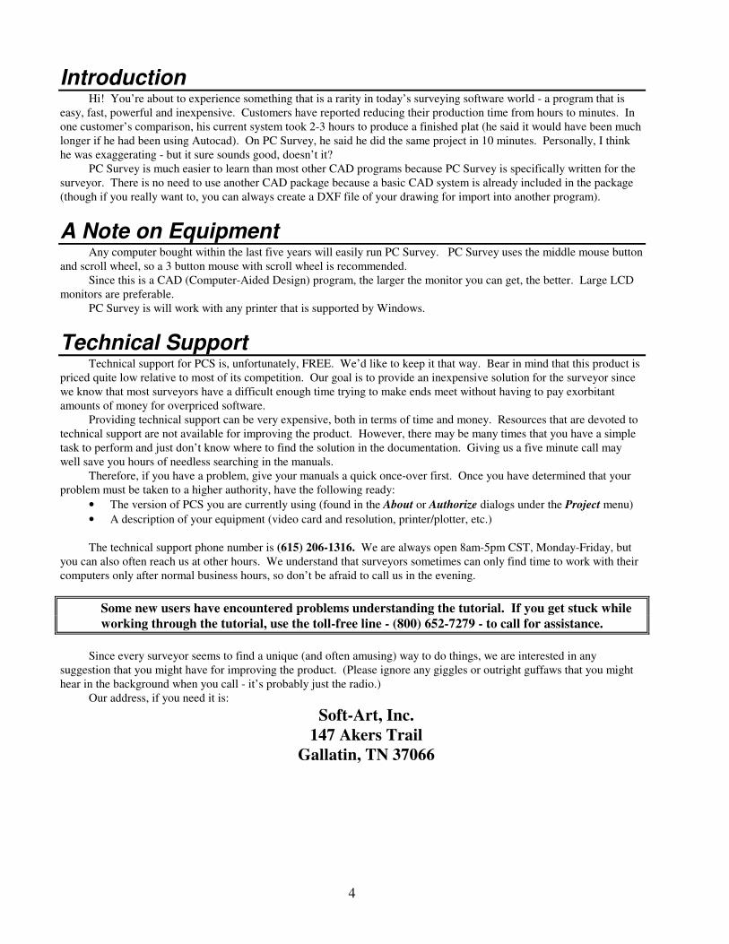
Introduction Hi! You’re about to experience something that is a rarity in today’s surveying software world - a program that is
easy, fast, powerful and inexpensive. Customers have reported reducing their production time from hours to minutes. In
one customer’s comparison, his current system took 2-3 hours to produce a finished plat (he said it would have been much
longer if he had been using Autocad). On PC Survey, he said he did the same project in 10 minutes. Personally, I think
he was exaggerating - but it sure sounds good, doesn’t it?
PC Survey is much easier to learn than most other CAD programs because PC Survey is specifically written for the
surveyor. There is no need to use another CAD package because a basic CAD system is already included in the package
(though if you really want to, you can always create a DXF file of your drawing for import into another program).
A Note on Equipment Any computer bought within the last five years will easily run PC Survey. PC Survey uses the middle mouse button
and scroll wheel, so a 3 button mouse with scroll wheel is recommended.
Since this is a CAD (Computer-Aided Design) program, the larger the monitor you can get, the better. Large LCD
monitors are preferable.
PC Survey is will work with any printer that is supported by Windows.
Technical Support Technical support for PCS is, unfortunately, FREE. We’d like to keep it that way. Bear in mind that this product is
priced quite low relative to most of its competition. Our goal is to provide an inexpensive solution for the surveyor since
we know that most surveyors have a difficult enough time trying to make ends meet without having to pay exorbitant
amounts of money for overpriced software.
Providing technical support can be very expensive, both in terms of time and money. Resources that are devoted to
technical support are not available for improving the product. However, there may be many times that you have a simple
task to perform and just don’t know where to find the solution in the documentation. Giving us a five minute call may
well save you hours of needless searching in the manuals.
Therefore, if you have a problem, give your manuals a quick once-over first. Once you have determined that your
problem must be taken to a higher authority, have the following ready:
• The version of PCS you are currently using (found in the About or Authorize dialogs under the Project menu)
• A description of your equipment (video card and resolution, printer/plotter, etc.)
The technical support phone number is (615) 206-1316. We are always open 8am-5pm CST, Monday-Friday, but
you can also often reach us at other hours. We understand that surveyors sometimes can only find time to work with their
computers only after normal business hours, so don’t be afraid to call us in the evening.
Some new users have encountered problems understanding the tutorial. If you get stuck while
working through the tutorial, use the toll-free line - (800) 652-7279 - to call for assistance.
Since every surveyor seems to find a unique (and often amusing) way to do things, we are interested in any
suggestion that you might have for improving the product. (Please ignore any giggles or outright guffaws that you might
hear in the background when you call - it’s probably just the radio.)
Our address, if you need it is:
Soft-Art, Inc.
147 Akers Trail
Gallatin, TN 37066
5
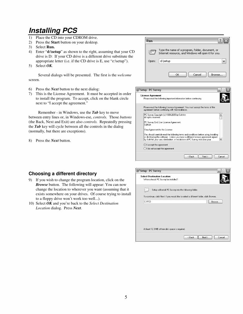
Installing PCS 1) Place the CD into your CDROM drive.
2) Press the Start button on your desktop.
3) Select Run.
4) Enter “d:\setup” as shown to the right, assuming that your CD
drive is D: If your CD drive is a different drive substitute the
appropriate letter (i.e. if the CD drive is E, use “e:\setup”).
5) Select OK.
Several dialogs will be presented. The first is the welcome
screen.
6) Press the Next button to the next dialog:
7) This is the License Agreement. It must be accepted in order
to install the program. To accept, click on the blank circle
next to “I accept the agreement.”
Remember - in Windows, use the Tab key to move
between entry lines or, in Windows-ese, controls. Those buttons
(the Back, Next and Exit) are also controls. Repeatedly pressing
the Tab key will cycle between all the controls in the dialog
(normally, but there are exceptions).
8) Press the Next button.
Choosing a different directory
9) If you wish to change the program location, click on the
Browse button. The following will appear: You can now
change the location to wherever you want (assuming that it
exists somewhere on your drives. Of course trying to install
to a floppy drive won’t work too well...).
10) Select OK and you’re back to the Select Destination
Location dialog. Press Next.
6
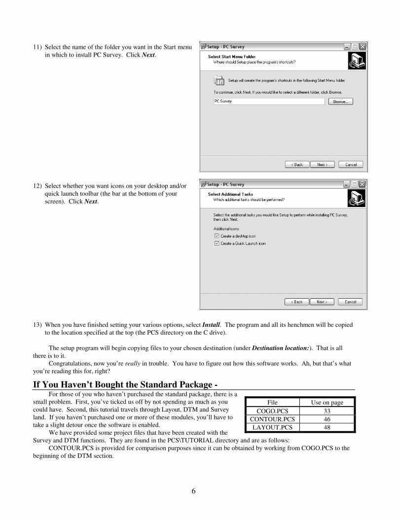
11) Select the name of the folder you want in the Start menu
in which to install PC Survey. Click Next.
12) Select whether you want icons on your desktop and/or
quick launch toolbar (the bar at the bottom of your
screen). Click Next.
13) When you have finished setting your various options, select Install. The program and all its henchmen will be copied
to the location specified at the top (the PCS directory on the C drive).
The setup program will begin copying files to your chosen destination (under Destination location:). That is all
there is to it.
Congratulations, now you’re really in trouble. You have to figure out how this software works. Ah, but that’s what
you’re reading this for, right?
If You Haven’t Bought the Standard Package - For those of you who haven’t purchased the standard package, there is a
small problem. First, you’ve ticked us off by not spending as much as you
could have. Second, this tutorial travels through Layout, DTM and Survey
land. If you haven’t purchased one or more of these modules, you’ll have to
take a slight detour once the software is enabled.
We have provided some project files that have been created with the
Survey and DTM functions. They are found in the PCS\TUTORIAL directory and are as follows:
CONTOUR.PCS is provided for comparison purposes since it can be obtained by working from COGO.PCS to the
beginning of the DTM section.
File Use on page
COGO.PCS 33
CONTOUR.PCS 46
LAYOUT.PCS 48
7
Authorizing PCS The program has not yet been authorized. As installed, PC Survey will not allow access to any windows except for
Cogo. This is an attempt to discourage those who feel that there is nothing wrong with using the hard work of others for
their own profit (thence the appellation - software pirate).
Since an authorization code is required to make this program usable to demo or for production work, feel free to
give copies of CD to your friends along with our phone number. They can call us for a temporary authorization if they
wish to play with the program.
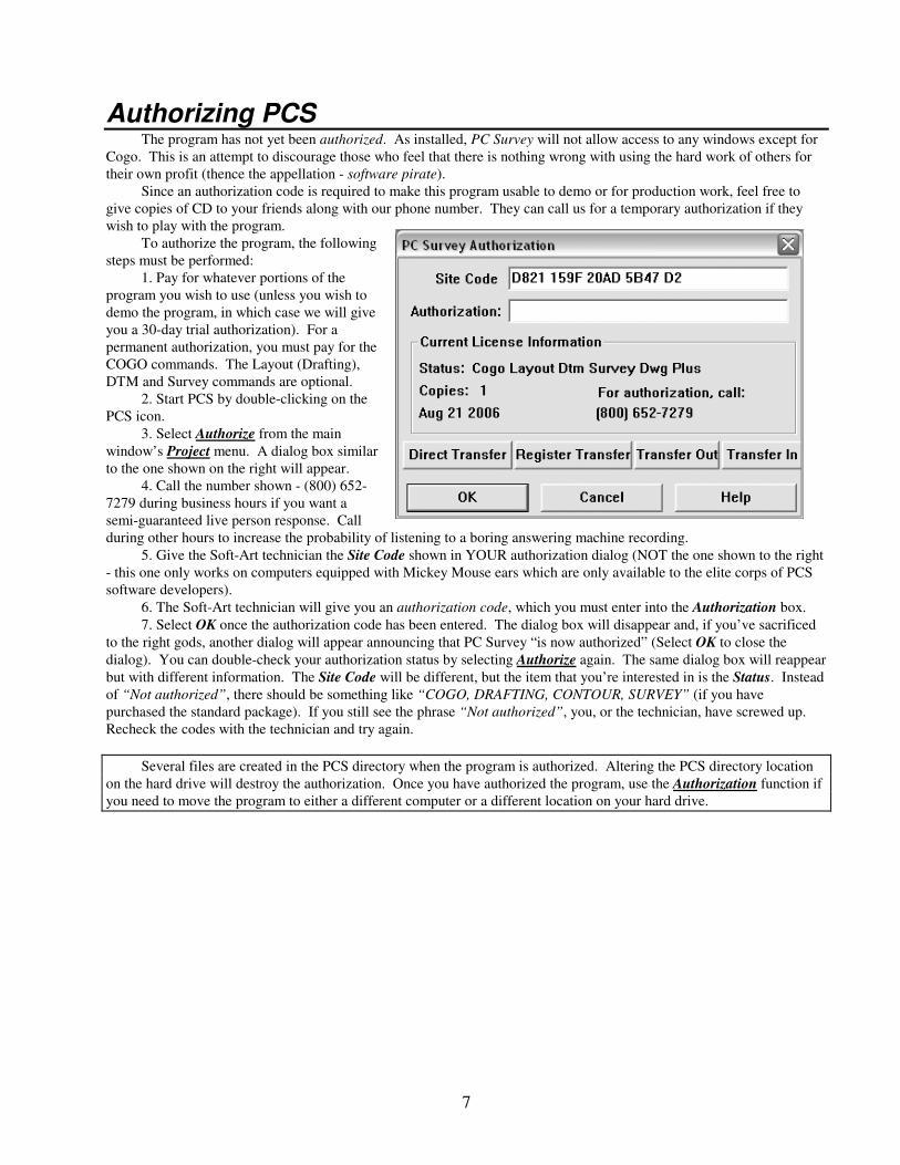
To authorize the program, the following
steps must be performed:
1. Pay for whatever portions of the
program you wish to use (unless you wish to
demo the program, in which case we will give
you a 30-day trial authorization). For a
permanent authorization, you must pay for the
COGO commands. The Layout (Drafting),
DTM and Survey commands are optional.
2. Start PCS by double-clicking on the
PCS icon.
3. Select Authorize from the main
window’s Project menu. A dialog box similar
to the one shown on the right will appear.
4. Call the number shown - (800) 652-
7279 during business hours if you want a
semi-guaranteed live person response. Call
during other hours to increase the probability of listening to a boring answering machine recording.
5. Give the Soft-Art technician the Site Code shown in YOUR authorization dialog (NOT the one shown to the right
- this one only works on computers equipped with Mickey Mouse ears which are only available to the elite corps of PCS
software developers).
6. The Soft-Art technician will give you an authorization code, which you must enter into the Authorization box.
7. Select OK once the authorization code has been entered. The dialog box will disappear and, if you’ve sacrificed
to the right gods, another dialog will appear announcing that PC Survey “is now authorized” (Select OK to close the
dialog). You can double-check your authorization status by selecting Authorize again. The same dialog box will reappear
but with different information. The Site Code will be different, but the item that you’re interested in is the Status. Instead
of “Not authorized”, there should be something like “COGO, DRAFTING, CONTOUR, SURVEY” (if you have
purchased the standard package). If you still see the phrase “Not authorized”, you, or the technician, have screwed up.
Recheck the codes with the technician and try again.
Several files are created in the PCS directory when the program is authorized. Altering the PCS directory location
on the hard drive will destroy the authorization. Once you have authorized the program, use the Authorization function if
you need to move the program to either a different computer or a different location on your hard drive.

8
Windows Concepts This section will be a basic review of Microsoft Windows terminology, concepts and operating procedures. If you
are already familiar with Microsoft Windows, you can probably skip to the next section. Alternatively, you can read your
Microsoft Windows manual to obtain a more detailed explanation.
Mouse Terminology You’ll see the following terms used frequently.
Click To quickly press and release the mouse button. When used by
itself, this term applies to the left mouse button. Sometimes, this
term will be qualified by the terms Left-click, Right-click or
Middle-click to refer specifically to one of the three mouse buttons.
Double-click To click the mouse button twice in rapid succession.
Drag To hold down the mouse button while you move the mouse.
Click and drag To press the mouse button (click) and hold the mouse button down
while moving the mouse. This term might be qualified by
specifying which button to use, as in Right-click and drag.
Windows - Moving, Resizing, Closing Not all windows have the same elements, but most have certain elements in common, such as title bars and menus.
The picture shown is the window used by the Notepad program that comes with Windows. (Notepad is a primitive text
editor).
The Control menu box is in the upper left
corner of each window.
The title bar displays the name of the
document. In this case the bar is where the window
title name, “Untitled - Notepad” sits.
The menu bar, under the title bar, lists the
available menus that contain lists of commands.
The window border is the outside edge of the
window. When the cursor is on the border, it will
look like a pair of opposite facing arrows. The
arrows indicate the direction in which you can move
the border to change the size of the window. Moving
the border is accomplished by clicking with the left
button of the mouse, and holding it down while
dragging the border to its new position. This kind of
mouse operation is called a click and drag. The
click and drag technique is VERY important to the operation of PCS.
The window corner can be used to shorten or lengthen two sides by again clicking and dragging.
The insertion point or focus indicates where you are in a document and is represented by a short, vertical blinking
line.
The Maximize button is in the upper right corner of the window and is represented by a box. Clicking on the
maximize button will enlarge the window to fill the screen.
When the window is maximized, the Restore button will appear in the upper right instead of the Maximize button.
Clicking on this button restores the window to its previous size and location. The Restore button is a double box.
The Minimize button is also in the upper right corner of the window to the left of the maximize button (the short
line). Clicking on the minimize button will reduce the window to an icon.
The client area is the now empty space inside the frame.
Certain techniques are used to manipulate a window:
• To click on a selected or chosen item or word or place, quickly press and release the mouse button.

9
• Double clicking means to click the mouse button twice in quick succession.
• To drag, hold down the left mouse button while moving the mouse.
• To point, move the mouse until the mouse pointer on the screen is on the chosen item.
• Selecting is to mark an item with a selection cursor, which can appear as a highlight, a dotted rectangle or both.
Selecting alone does not start an action.
• Choosing an item is to initiate an action.
• Zooming is to change the amount of data visible in the window by magnifying or reducing the view.
• To move a window to any location on the desktop, just click on the title bar and drag to the desired location.
Release the mouse button. If the action is to be canceled, press <Esc> before the mouse button is released.
• To change the size of a window, select the desired window, point to a border where the pointer will turn into a
double-headed arrow, and drag the corner or border until the window is the needed size.
• To enlarge an application window, select the desired window and click the Maximize button in the upper right
corner of the window.
• To close a window, choose Exit from the File menu, or choose Close from the Control menu, or, as a shortcut,
double-click the Control-menu box.
Menus Each application has a list of commands called “Menus” found in the Menu bar at the upper edge of the application
window. When a menu is selected, a list of other commands appears in a small box. Choosing one of those commands
carries out an action.
To select a menu, click on the appropriate menu to open it up. To close the menu, click the menu name or anywhere
outside the menu. To remain in the menu bar with the menu closed, press <Esc>.
As mentioned earlier, menus have a list of commands but they also can have a list of characteristics assigned to
graphics or text, a list of open windows or files, or the names of cascading menus, which have more commands.
Dialogs A dialog box requests information about a project or supplies needed information. Most dialogs (dialog boxes) have
options that can be selected. Other dialogs have additional information, warnings or messages showing why a requested
task cannot be done.
There can be several types of options or controls within a dialog box. Some are in the form of buttons, as shown in
the above example, such as the OK button which carries out the command you choose or the Cancel button which cancels
the command you choose or the Display button which will bring up a list of stake points and the Select File button. To
choose a command button, simply click on it with the mouse. The keyboard can also be used by pressing TAB to move to
the button desired and then pressing the SPACE bar. If the button or option has an underlined letter in it, just type that
letter while holding down the ALT key.

10
In the above example you will find some typical controls, most of which are in edit or text boxes. The terms edit
box and text box can be used interchangeably - they’re the same thing. All the white boxes, except the Direction box,
require typed in information and are called edit boxes. The edit box titled Output has two sets of radio buttons; only one
button of each set can be on at any given time. In this case, Table was chosen rather than Delimited ASCII and By
Direction instead of Tangent Offsets. The white box labeled Angle format and followed by a down arrow button is a
drop-down list. When the button is pressed, a list of choices will appear. The Create COGO points box is called a check
box because, if you click on it, a check will appear in the little box; if you click on it a second time, the check will
disappear.
Focus - this is an important term to understand. When in a dialog, one of the controls (buttons, edit box, checkbox,
etc.) will be considered to have the focus, meaning that any input will be directed at that control. When an edit box has
the focus, for instance, there will either be an insertion cursor in the edit box (a vertical bar) or the text in the edit box will
be highlighted in blue. When buttons and checkboxes have the focus, their text (title or caption - such as Create COGO
points in the above picture) will have a light rectangle around it.
To choose any of these options with the mouse, click on the selected box. Or, with the keyboard, press <TAB> (the
Tab key on your keyboard - keyboard keys will be designated by <key> throughout this manual) to move to the group of
options desired, use the arrow keys to select the appropriate button, and then press <ENTER>.
To move a dialog, drag the title bar to the desired location with the mouse.
To move around inside a dialog, click the desired option or space to which to move or, when not using the mouse,
press <TAB> to move forward (from left to right and top to bottom). Press <SHIFT > + <TAB> to move in the opposite
direction. Use the arrow keys to move from one option to another within an area.
11
Fire it up! OK, we’re ready to begin. Sit back and move the mouse cursor over the PCS icon. Double-click it - CAREFULLY!
There’s a lot of horsepower under the hood of this thing.
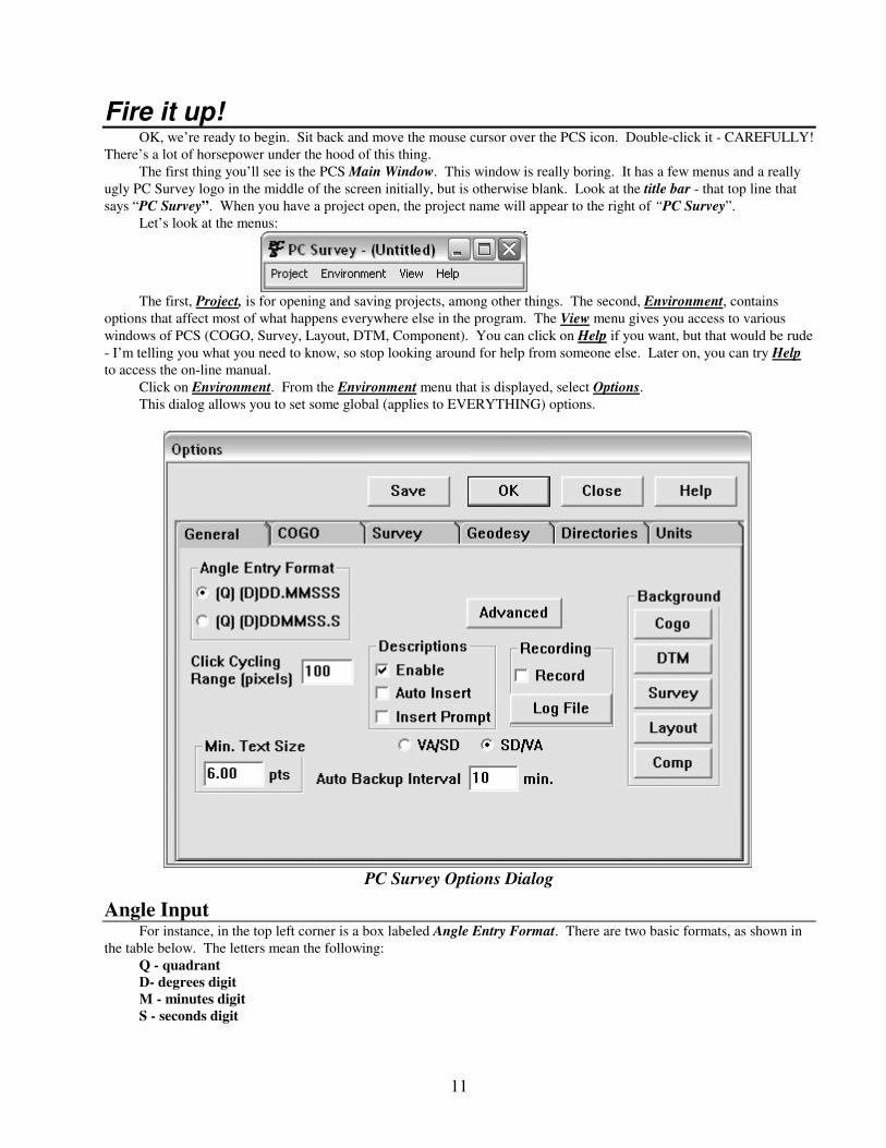
The first thing you’ll see is the PCS Main Window. This window is really boring. It has a few menus and a really
ugly PC Survey logo in the middle of the screen initially, but is otherwise blank. Look at the title bar - that top line that
says “PC Survey”. When you have a project open, the project name will appear to the right of “PC Survey”.
Let’s look at the menus:
The first, Project, is for opening and saving projects, among other things. The second, Environment, contains
options that affect most of what happens everywhere else in the program. The View menu gives you access to various
windows of PCS (COGO, Survey, Layout, DTM, Component). You can click on Help if you want, but that would be rude
- I’m telling you what you need to know, so stop looking around for help from someone else. Later on, you can try Help
to access the on-line manual.
Click on Environment. From the Environment menu that is displayed, select Options.
This dialog allows you to set some global (applies to EVERYTHING) options.
PC Survey Options Dialog
Angle Input For instance, in the top left corner is a box labeled Angle Entry Format. There are two basic formats, as shown in
the table below. The letters mean the following:
Q - quadrant
D- degrees digit
M - minutes digit
S - seconds digit

12
The quadrant is an optional field (that is why it is in parentheses) that only applies to the input of bearings. Bearing
input in PCS can be done in many ways. Examples for entering the bearing S58°°°°46’39.2”E are:
This tutorial will assume that the first format (the left
column) will be used when entering angles. If your personal
preference is to use the second format, you can change it by
clicking on the radio button next to that format (as shown on
the right). Use the other settings as shown.
The Directories settings determine where PCS will
initially look when attempting to open project and library
files.
1) Select the Directories tab
near the top of the dialog. A
dialog similar to the one
shown will appear. We want
to change the Project
directory setting to the
C:\PCS\TUTORIAL
directory. If you used the
default installation settings,
PCS is installed on the C
drive in the root (top level)
directory.
2) Change the path shown in the
dialog for the Project
directory to the PCS/TUTORIAL directory using the Browse function.
3) Click Save to save the settings.
4) Select OK to close the dialog.
Opening a window Click on View. You should now see a submenu, a vertical menu list. At the top of the list is
COGO. This is a list of PCS window names. Clicking on the name of a window in this dialog will
bring it to the front so you can see it (sometimes they can be a bit shy). DON’T CLICK ON
ANYTHING YET! If you did, you might have ignited the delayed self-destruct! (destructive
radius of two disk partitions) Click on the line that says COGO to bring up the PCS COGO
window OR press the F2 key on your keyboard. The F2 key is called an accelerator - it is a
shortcut keystroke sequence to the COGO function. Functions that have accelerators will list the
accelerator next to the function name in the menus (F9 is the accelerator for the Edit Layers
function, for example).
Entering S58°°°°46’39.2”E
(Q) (D)DD.MMSSS (Q) (D)DDMMSS.S
2 58.46392
or 2.58.46392
2 584639.2
or 2.584639.2
58.46392 584639.2
S58.46392E S584639.2E
View Menu
13
The COGO Window
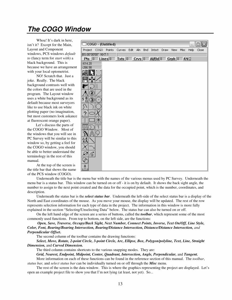
Whoa! It’s dark in here,
isn’t it? Except for the Main,
Layout and Component
windows, PCS windows default
to (fancy term for start with) a
black background. This is
because we have an arrangement
with your local optometrist.
NO! Scratch that. Just a
joke. Really. The black
background contrasts well with
the colors that are used in the
program. The Layout window
uses a white background as its
default because most surveyors
like to use black ink on white
plotting paper (no imagination,
but most customers look askance
at fluorescent orange paper).
Let’s discuss the parts of
the COGO Window. Most of
the windows that you will see in
PC Survey will be similar to this
window so, by getting a feel for
the COGO window, you should
be able to better understand the
terminology in the rest of this
manual.
At the top of the screen is
the title bar that shows the name
of the PCS window (COGO).
Underneath the title bar is the menu bar with the names of the various menus used by PC Survey. Underneath the
menu bar is a status bar. This window can be turned on or off - it is on by default. It shows the back sight angle, the
number to assign to the next point created and the data for the occupied point, which is the number, coordinates, and
description.
Underneath the status bar is the select status bar. Underneath the left-side of the select status bar is a display of the
North and East coordinates of the mouse. As you move your mouse, the display will be updated. The rest of the row
represents selection information for each type of data in the project. The information in this window is more fully
explained in the section “Selecting/Unselecting Data” below. The status bar can also be turned on or off.
On the left hand edge of the screen are a series of buttons, called the toolbar, which represent some of the most
commonly used functions. From top to bottom, on the left side, are the functions:
Open, Save, Traverse, Occupy/Back Sight, Next Number, Connect Points, Inverse, Text On/Off, Line Style,
Color, Font, Bearing/Bearing Intersection, Bearing/Distance Intersection, Distance/Distance Intersection, and
Perpendicular Offset.
The second column of the toolbar contains the drawing functions:
Select, Move, Rotate, 2-point Circle, 3-point Circle, Arc, Ellipse, Box, Polygon/polyline, Text, Line, Straight
Dimension, and Curved Dimension.
The third column contains shortcuts to the various snapping modes. They are:
Grid, Nearest, Endpoint, Midpoint, Center, Quadrant, Intersection, Angle, Perpendicular, and Tangent.
More information on each of these functions can be found in the reference section of this manual. The toolbar,
status bar, and select status bar can be individually turned on or off through the Misc menu.
The rest of the screen is the data window. This is where the graphics representing the project are displayed. Let’s
open an example project file to show you that I’m not lying (at least, not yet). So...

14
Move the mouse cursor on top of the top left button in the toolbar (the picture of a file folder with PCS underneath
it). This is the Open function that is also accessible from the Project menu. Notice the bold, italic underlining that was
used. When you see this (Connect Points is another example), you know that a menu function is being discussed.
With the mouse cursor over the Open button, depress the left button. A dialog (a box with various controls such as
edit boxes, checkboxes, and
buttons) will appear on the screen
similar to the one shown, except
that the current directory will be
proj if you haven’t changed the
default directory as mentioned
earlier.
This is your basic Windows
file dialog, used for selecting files
from the hard drive. To show
how this works, we will change to
the c:\pcs\tutorial directory by
doing the following:
1) Press the button to the
right of the “Look in”
list. The button has a
picture of a folder with
an “up” arrow on it.
The list will change
and you should now
see a directory (folder)
labeled tutorial.
2) Move the cursor onto the line labeled tutorial and double-click with the left mouse button again. This will
change the current directory (the one displayed in the “Look in” list) to tutorial and the dialog should appear
similar to the one shown above.
In this case we want to open the EXAMPLE1.PCS file that exists in the TUTORIAL directory underneath your PCS
directory.
To review this procedure, it goes like this:
To the right of Look in: is current path (in the picture it is Tutorial).
Underneath the current path is a representation of the directory structure for this path. The picture to the left of the
texts are supposed to look like a sheet of paper, if the item is a file. If the item is a directory/folder, the picture to the left
will look like a folder. There are no directories underneath (contained in)
tutorial, so there are no folders displayed in the list.
On the bottom is an edit box for entering a file name. Underneath it
is a list of the files in the current directory that match the specification in
the File Name box. Notice that the file name defaults to *.pcs;*.ces so
that the list includes only those files that end with .pcs or .ces. The “*”
(asterisk) in front of the “.pcs” is called a wildcard and means “any
sequence of characters.”
Open the EXAMPLE1.PCS job by double-clicking on the
example1.pcs name in the file list box (right there below contour.pcs and
above layout.pcs. It’s two below cogo.pcs on the far left of the dialog box
just above the center. The OK button is on the opposite side of the box. If
you’re in Paris walking along the Louvre, you’re not even close to where
you need to be.)
The Open Project dialog will automatically close if you double-click
on the file name. If you single-click, the name will be placed in the File
Name box. You can then click on the OK button to complete the
operation. There may be a short delay depending on how fast your
computer is, but a message that says “Loading, please wait...” should
appear. The message will disappear when the project has been loaded.
The program will then draw the project in the COGO window.
There are many details that will not be visible until you zoom in (get
The Example1 project in COGO
15
closer). For example, there are many texts along the lines in the drawing that you can’t see at this magnification (unless
you’re using a high-resolution display mode).
We’re going to use this example to demonstrate some of the functions of the program. Before making any changes
to this file, we should probably first save it to a different file in order to keep the original intact (just in case you want to
go through this portion of the
tutorial again).
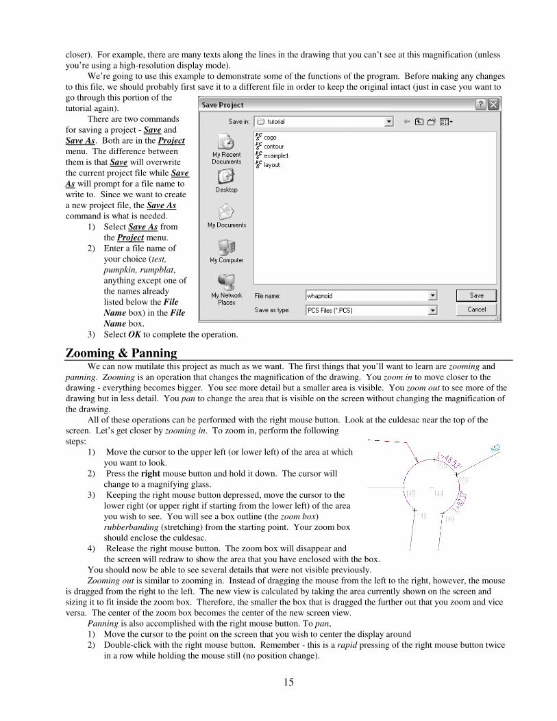
There are two commands
for saving a project - Save and
Save As. Both are in the Project
menu. The difference between
them is that Save will overwrite
the current project file while Save
As will prompt for a file name to
write to. Since we want to create
a new project file, the Save As
command is what is needed.
1) Select Save As from
the Project menu.
2) Enter a file name of
your choice (test,
pumpkin, rumpblat,
anything except one of
the names already
listed below the File
Name box) in the File
Name box.
3) Select OK to complete the operation.
Zooming & Panning We can now mutilate this project as much as we want. The first things that you’ll want to learn are zooming and
panning. Zooming is an operation that changes the magnification of the drawing. You zoom in to move closer to the
drawing - everything becomes bigger. You see more detail but a smaller area is visible. You zoom out to see more of the
drawing but in less detail. You pan to change the area that is visible on the screen without changing the magnification of
the drawing.
All of these operations can be performed with the right mouse button. Look at the culdesac near the top of the
screen. Let’s get closer by zooming in. To zoom in, perform the following
steps:
1) Move the cursor to the upper left (or lower left) of the area at which
you want to look.
2) Press the right mouse button and hold it down. The cursor will
change to a magnifying glass.
3) Keeping the right mouse button depressed, move the cursor to the
lower right (or upper right if starting from the lower left) of the area
you wish to see. You will see a box outline (the zoom box)
rubberbanding (stretching) from the starting point. Your zoom box
should enclose the culdesac.
4) Release the right mouse button. The zoom box will disappear and
the screen will redraw to show the area that you have enclosed with the box.
You should now be able to see several details that were not visible previously.
Zooming out is similar to zooming in. Instead of dragging the mouse from the left to the right, however, the mouse
is dragged from the right to the left. The new view is calculated by taking the area currently shown on the screen and
sizing it to fit inside the zoom box. Therefore, the smaller the box that is dragged the further out that you zoom and vice
versa. The center of the zoom box becomes the center of the new screen view.
Panning is also accomplished with the right mouse button. To pan,
1) Move the cursor to the point on the screen that you wish to center the display around
2) Double-click with the right mouse button. Remember - this is a rapid pressing of the right mouse button twice
in a row while holding the mouse still (no position change).

16
Practice zooming and panning until you are comfortable with these operations.
Zoom Previous, Full View and Redraw There are three functions that affect the display that are highly useful. They are found in the View menu.
Zoom Previous will revert the displayed area to whatever it was before the last zoom or pan. It has an accelerator -
Ctrl-Shift-F8. An accelerator, if you don’t recall, is a keyboard sequence that can be used to access a menu function
generally more quickly than selecting the function from the menu. When an accelerator includes more than one key, as in
this case, pressing and holding the buttons down in the order specified execute it. In this case, you would depress and
hold the Ctrl key followed by depressing and holding the Shift key and finally depressing the F8 key.
Full View is a quick way to zoom out to the point where the whole drawing is displayed. Its accelerator is Shift-F8.
Redraw is used to regenerate the drawing on the screen. This is useful because various functions can partially
scramble the screen drawing. The screen drawing may also be incomplete due to interrupted drawing. The Redraw
accelerator is F8.
Speaking of interrupted drawing - some computers can be very slow in drawing the screen (386s in particular).
Sometimes, you may execute a zoom or pan and not need a complete redraw of the screen.
Screen redraw can usually be stopped by pressing the <Esc> key.
Play with these functions awhile until you are comfortable with them.
Selecting & Unselecting Now for some other VERY important concepts. Most of the functions in PCS operate on what is called a select list.
The select list is simply the set of objects (lines, points, arcs, etc.) that are currently selected. Selected objects will be
displayed with some sort of special highlighting, shading or cross-hatching.
For instance, to change the point symbol of a set of points, you first select the points that are to be modified and then
execute, in this case, the Modify Group function from the Points menu in COGO. We’ll get to that one in a bit. First let’s
discuss how selecting/unselecting is performed.
Selecting is very similar to the zoom in operation. Instead of using the right mouse button, however, you use the left
mouse button. It goes like this:
1) Move the cursor to the upper left (or lower left) of the area that you want to select.
2) Press the left mouse button and hold it down
3) Keeping the left mouse button depressed, move the cursor to the lower right (or upper right if starting from the
lower left) of the area you wish to select. You will see a box outline (the select box) rubberbanding (stretching)
from the starting point.
4) Release the left mouse button. The select box will disappear and the selected objects will be redrawn with
highlighting.
Every object that is enclosed, touched or crossed by the selection box is a candidate for selection. They are
candidates because they are selected only if they are selectable. Whether an object is selectable depends on two things:
•It must be visible (visible objects might not necessarily be visible on the screen if zoomed out).
•It must be within the selection criterion of the object selection filters.
The selection filters are controlled through the select status bar - the third line at the top of the screen. We’ll talk
about them later. Notice for now that, when you select things, the numbers next to the buttons in the select status bar (Pts,
Lines, Crv, etc.) change to show the number of each type of object currently selected.
Unselecting is the same operation as selecting except that, instead of dragging the selection box from the left to
right, you drag the box from right to left.
Select by left-clicking and dragging from left to right.
Unselect by left-clicking and dragging from right to left.
Practice selecting and unselecting with the selection box until (you guessed it) you are comfortable.
Sometimes you may wish to select a single item from a closely drawn group of objects. Dragging a selection box
won’t allow you to get JUST that one item. In this case, you can use what is called a point select. This operation is
performed with a single click and release with the left mouse button. The trick is in not moving the mouse while doing
this.
When performing a point select, the first left-click will select the nearest selectable object. If this is not the desired
object, repeating the left-click without moving the mouse will unselect the first object and find the next nearest object.
The next left-click will unselect that object and find the third nearest selectable object and so forth. Each successive point
17
select will search outwards for selectable objects until no more can be found within the Click Cycling Range (specified in
the Environment - Options dialog). At that point the search begins over again with the nearest selectable object.
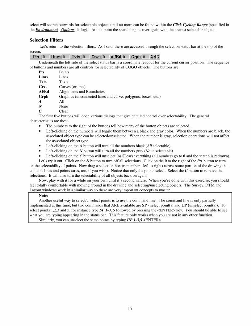
Selection Filters
Let’s return to the selection filters. As I said, these are accessed through the selection status bar at the top of the
screen.
Underneath the left side of the select status bar is a coordinate readout for the current cursor position. The sequence
of buttons and numbers are all controls for selectability of COGO objects. The buttons are
Pts Points
Lines Lines
Txts Texts
Crvs Curves (or arcs)
Al/Bd Alignments and Boundaries
Grph Graphics (unconnected lines and curve, polygons, boxes, etc.)
A All
N None
C Clear
The first five buttons will open various dialogs that give detailed control over selectability. The general
characteristics are these:
• The numbers to the right of the buttons tell how many of the button objects are selected..
• Left-clicking on the numbers will toggle them between a black and gray color. When the numbers are black, the
associated object type can be selected/unselected. When the number is gray, selection operations will not affect
the associated object type.
• Left-clicking on the A button will turn all the numbers black (All selectable).
• Left-clicking on the N button will turn all the numbers gray (None selectable).
• Left-clicking on the C button will unselect (or Clear) everything (all numbers go to 0 and the screen is redrawn).
Let’s try it out. Click on the N button to turn off all selections. Click on the 0 to the right of the Pts button to turn
on the selectability of points. Now drag a selection box (remember - left to right) across some portion of the drawing that
contains lines and points (arcs, too, if you wish). Notice that only the points select. Select the C button to remove the
selections. It will also turn the selectability of all objects back on again.
Now, play with it for a while on your own until it’s second nature. When you’re done with this exercise, you should
feel totally comfortable with moving around in the drawing and selecting/unselecting objects. The Survey, DTM and
Layout windows work in a similar way so these are very important concepts to master.
Note:
Another useful way to select/unselect points is to use the command line. The command line is only partially
implemented at this time, but two commands that ARE available are SP - select point(s) and UP (unselect point(s)). To
select points 1,2,3 and 5, for instance type SP 1-3, 5 followed by pressing the <ENTER> key. You should be able to see
what you are typing appearing in the status bar. This feature only works when you are not in any other function.
Similarly, you can unselect the same points by typing UP 1-3,5 <ENTER>.

18
Moving, Rotating and Resizing Text One of PCS’s simpler, yet powerful, features is the ability to visually move and rotate texts. With the exception of
the default point and curve annotation, all texts can be moved and rotated with the mouse. The procedure is the following:
To move a text:
1) Select it.
2) Place the cursor on the text (anywhere within the rectangular area that includes the text).
3) Depress the left button of the mouse and hold it down while NOT MOVING THE MOUSE. After a short
delay, the text will disappear and a rectangular outline box will take its place.
4) With the mouse button still depressed, move the mouse. The outline box will move with the cursor.
5) When the outline box is in the desired location, release the left mouse button. The text will reappear in its new
position.
To rotate a text:
1) Perform steps 1 and 5 as above EXCEPT, in step 3, depress and hold the Ctrl key on the keyboard before
depressing the left mouse button. Hold this key down until the rotation is complete.
Practice on some of the bearing or distance texts in the example project. Notice that you can’t move or rotate the
point numbers (though there is an easy way to make this possible) or the curve text.
Changing the size of text is a common operation when modifying a drawing. The move and rotate functions operate
on a single text at a time, but changing text size is performed using the Set Font function that operates on all texts in the
selection list. You can therefore select several texts and change their sizes (and font) in a single step.
To change a font:
1) Select one or more of the bearing/distance texts in the example project.
2) Either select the Set Font-Other function from the Edit menu or press the Set Font button in the
toolbar. A dialog similar to the one shown below will appear. In this dialog you can alter both the
font and size of the text.
3) Change the Size value to something large - say 0.25 (quarter inch).
4) Select OK to close the dialog. The screen will redraw and the selected texts should be much larger
than they were.
Notes: • When using a raster-type printer
(inkjet, laser, dot matrix,
thermal), you can use virtually
any font that is installed on the
system.
• Precise text alignment can be
performed with the Text Align
function or by using the
Snapping functions. Refer to the
reference manual for more
information.
Set Font
button
19
Some COGO Point Functions In this section we’ll play with some of COGO’s point functions. You’ll be using the zoom/pan and selection
functions you have just learned.
Points have several characteristics that can be modified. In addition to their basic data values (number, northing,
easting, elevation, and description), points have a symbol, symbol size, layer, color and overlay. Like most PCS objects,
points can also be “hidden” or temporarily removed from view. The first functions we’ll examine are functions that
modify these characteristics.
As a guinea pig, we’ll use point 164. To modify this point, it first has to be selected. Though it is possible to select
the point without seeing it, we’ll practice using the select box technique. To use the select box, we must first be able to
see point 164. So where is it?
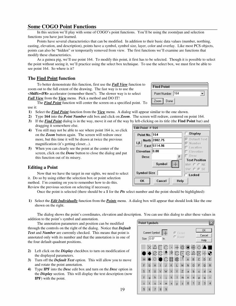
The Find Point function
To better demonstrate this function, first use the Full View function to
zoom out to the full extent of the drawing. The fast way is to use the
<Shift><F8> accelerator (remember them?). The slower way is to select
Full View from the View menu. Pick a method and DO IT!
The Find Point function will center the screen on a specified point. To
use it:
1) Select the Find Point function from the View menu. A dialog will appear similar to the one shown.
2) Type 164 into the Point Number edit box and click on Zoom. The screen will redraw, centered on point 164.
3) If the Find Point dialog is in the way, move it out of the way by left-clicking on its title (the Find Point bar) and
dragging it somewhere else.
4) You still may not be able to see where point 164 is, so click
on the Zoom button again. The screen will redraw once
more, but this time it will be drawn at twice the previous
magnification (it’s getting closer...).
5) When you can clearly see the point at the center of the
screen, click on the Done button to close the dialog and put
this function out of its misery.
Editing a Point
Now that we have the target in our sights, we need to select
it. Do so by using either the selection box or point selection
method. I’m counting on you to remember how to do this.
Review the previous section on selecting if necessary.
Once the point is selected (there should be a 1 for the Pts select number and the point should be highlighted):
1) Select the Edit Individually function from the Points menu. A dialog box will appear that should look like the one
shown on the right.
The dialog shows the point’s coordinates, elevation and description. You can use this dialog to alter these values in
addition to the point’s symbol and annotation.
The annotation parameters and position can be modified
through the controls on the right of the dialog. Notice that Default
Text and Number are currently checked. This means that point is
annotated only with its number and that the annotation is in one of
the four default quadrant positions.
2) Left click on the Display checkbox to turn on modification of
the displayed parameters.
3) Turn off the Default Text option. This will allow you to move
and rotate the point annotation.
4) Type IPF into the Desc edit box and turn on the Desc option in
the Display section. This will display the text description (now
IPF) with the point.

20
Let’s change the symbol.
5) Left-click on the Symbol button. Another dialog, the point symbol dialog, will appear. The first two rows of symbols
are standard stuff. The alphabetic characters following the first two rows are for assigning a circled or boxed
character symbol to the point.
6) Select the eighth symbol in the top row - (the double circle) and select OK to close this dialog.
7) Select OK in the Edit Point dialog to completely exit the function. Notice the changes that appear on screen.
You should now be able to select the point text (which now includes the description), move and rotate it like the
other bearing/distance texts.
By now, you should be getting a “feel” for how the system works.
The Command Line - a method for the keyboard addict.
In many instances, it is much faster and easier to enter commands directly instead of selecting functions from the menus
and filling in a dialog. For this reason, a command line has been included with PCS to expedite many of the functions.
Find Point is one of the functions that can be accessed through the command line. To illustrate,
1) Press <Shift><F8> to zoom the drawing back out.
2) Type FP 164 <Enter>. Notice that, as you type, the keystrokes are echoed (shown) in the status bar in place of the
occupied point status. The display will center on point 164 just as if the Find Point dialog had been used.
3) To zoom in further, type FP <Enter> or press <Spacebar><Enter>.
4) Repeat the previous step to continue zooming in on point 164.
Notice-
• Pressing <Spacebar> recalls the previous command.
The Edit Individually function also has a command line form. Its command is PE (Point Edit).
Example: Type PE 165<Enter> to see how this command works
Before moving on, select New from the Project menu to close this project and begin a new one.

21
The Survey Window
If you have not purchased the Survey module, go to p.33.
Now that you have seen the COGO window, let’s move to the Survey window. Select Survey from COGO’s View
menu OR press your <F4> key.
The Survey Window is used for field data entry and adjustment. Data entered in this window is stored with the
project so that you have a permanent record for future reference (at least until your 26,000 hour MTBF hard drive eats
itself after last night’s lightning strike). The Survey Window is also used for mapchecks.
As field data (or measurements, observations, shots - whatever) is entered, a graphics representation is drawn on the
screen. A basic measurement consisting of a horizontal angle and distance (plus, maybe, a vertical angle) is represented
on the screen as a line drawn from a station point to a foresight point. Points are a location represented by some symbol
such as a circle, a cross, an X, etc.
An Example Project It’s time to start working an example. The example is a property that is to be subdivided and have boundary
markers placed (monuments had been lost or never installed). Therefore, a traverse loop has to be created from the few
existing monuments before establishing the property boundaries. Below is a sketch of the property boundaries.
22
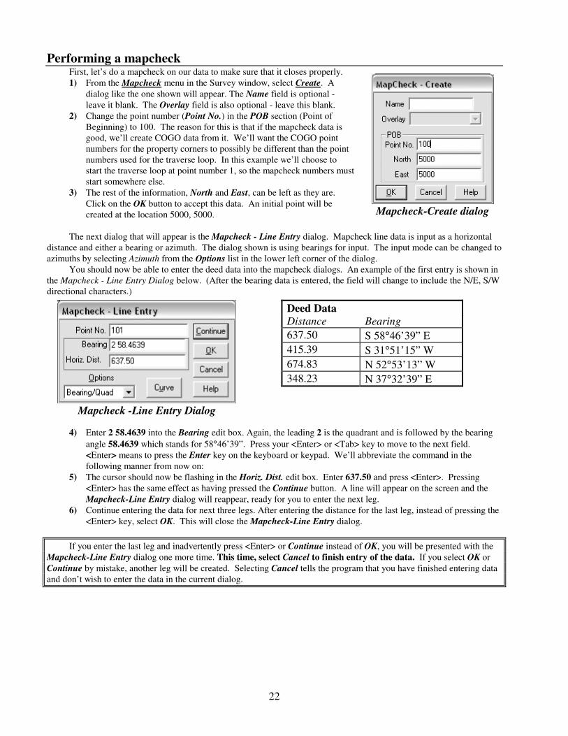
Performing a mapcheck First, let’s do a mapcheck on our data to make sure that it closes properly.
1) From the Mapcheck menu in the Survey window, select Create. A
dialog like the one shown will appear. The Name field is optional -
leave it blank. The Overlay field is also optional - leave this blank.
2) Change the point number (Point No.) in the POB section (Point of
Beginning) to 100. The reason for this is that if the mapcheck data is
good, we’ll create COGO data from it. We’ll want the COGO point
numbers for the property corners to possibly be different than the point
numbers used for the traverse loop. In this example we’ll choose to
start the traverse loop at point number 1, so the mapcheck numbers must
start somewhere else.
3) The rest of the information, North and East, can be left as they are.
Click on the OK button to accept this data. An initial point will be
created at the location 5000, 5000.
The next dialog that will appear is the Mapcheck - Line Entry dialog. Mapcheck line data is input as a horizontal
distance and either a bearing or azimuth. The dialog shown is using bearings for input. The input mode can be changed to
azimuths by selecting Azimuth from the Options list in the lower left corner of the dialog.
You should now be able to enter the deed data into the mapcheck dialogs. An example of the first entry is shown in
the Mapcheck - Line Entry Dialog below. (After the bearing data is entered, the field will change to include the N/E, S/W
directional characters.)
4) Enter 2 58.4639 into the Bearing edit box. Again, the leading 2 is the quadrant and is followed by the bearing
angle 58.4639 which stands for 58°46’39”. Press your <Enter> or <Tab> key to move to the next field.
<Enter> means to press the Enter key on the keyboard or keypad. We’ll abbreviate the command in the
following manner from now on:
5) The cursor should now be flashing in the Horiz. Dist. edit box. Enter 637.50 and press <Enter>. Pressing
<Enter> has the same effect as having pressed the Continue button. A line will appear on the screen and the
Mapcheck-Line Entry dialog will reappear, ready for you to enter the next leg.
6) Continue entering the data for next three legs. After entering the distance for the last leg, instead of pressing the
<Enter> key, select OK. This will close the Mapcheck-Line Entry dialog.
If you enter the last leg and inadvertently press <Enter> or Continue instead of OK, you will be presented with the
Mapcheck-Line Entry dialog one more time. This time, select Cancel to finish entry of the data. If you select OK or
Continue by mistake, another leg will be created. Selecting Cancel tells the program that you have finished entering data
and don’t wish to enter the data in the current dialog.
Mapcheck-Create dialog
Mapcheck -Line Entry Dialog
Deed Data
Distance Bearing
637.50 S 58°46’39” E
415.39 S 31°51’15” W
674.83 N 52°53’13” W
348.23 N 37°32’39” E
23
You can correct mistakes by selecting the mapcheck and then using the Edit command in the Mapcheck menu (after
finally selecting Cancel in the Mapcheck-Line Entry dialog) to invoke the mapcheck spreadsheet editor. The editor
allows you to modify any of your mapcheck data, including adding and deleting entries. Once all the mapcheck data has
been entered, you’ll want to generate a report in order to determine whether the deed data closed properly.
7) Select the mapcheck by doing the following:
To select the mapcheck: click the left button of the mouse and, while holding it down, drag the mouse to the right.
A selection box will be drawn on the screen as this is done. The selection box must either enclose or intersect an object in
order to select that object. In this case, the selection box needs to only cross any of the legs of the mapcheck in order to
select the mapcheck since the mapcheck is comprised of all the mapcheck legs. Release the left button after the selection
box has intersected the mapcheck (this is what is called a click and drag).
Selecting is a VERY common operation in PCS. Just as objects can be selected by dragging the selection box to the
right, objects can also be unselected by dragging the selection box to the left. Experiment with selecting and unselecting
till you are comfortable it. If this last sentence doesn’t sound familiar, then you are among naughty surveyors (ANaSs)
who skip the beginning of this tutorial. DON’T do it again. We’re watching you (and it’s not a pretty sight).
The loop should now be highlighted in bright yellow, with the first half of the first leg highlighted in white (this is
done to allow quick recognition of the first leg of a loop). One or more of the shots will also probably be selected -
they’re highlighted in red and may lie on top of the mapcheck loop’s highlighting (so you may see a red leg in the middle
of a yellow and white loop - right about now, you should be pining for the days of monochrome monitors). Additionally,
in the select status bar, the number 1 should appear to the right of the Loops button, showing that one loop (or mapcheck)
has been selected.
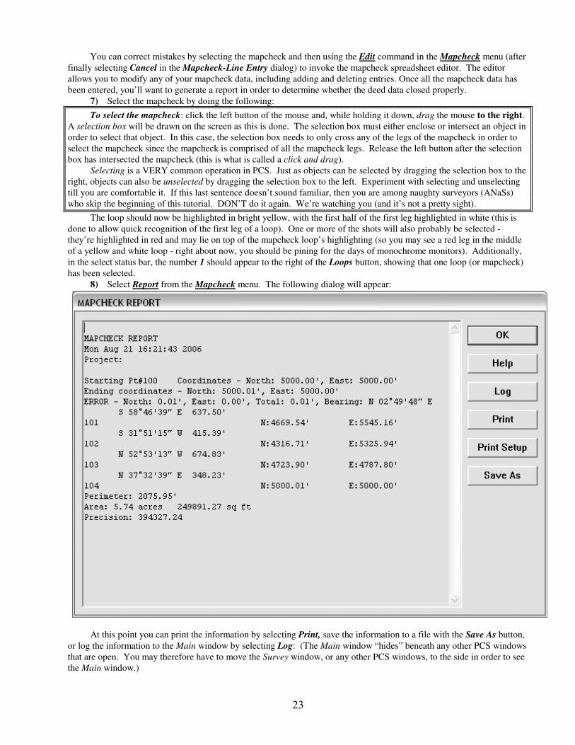
8) Select Report from the Mapcheck menu. The following dialog will appear:
At this point you can print the information by selecting Print, save the information to a file with the Save As button,
or log the information to the Main window by selecting Log: (The Main window “hides” beneath any other PCS windows
that are open. You may therefore have to move the Survey window, or any other PCS windows, to the side in order to see
the Main window.)

24
9) This looks pretty good so click on OK. The next step
is to transfer the mapcheck stuff (points, lines and
curves) to the COGO window so that it can be used
by the COGO functions. To do this,
10) If the mapcheck is not selected, use the procedure
above to reselect it.
11) Select To COGO from the Mapcheck menu. The
dialog shown to the right will be displayed. Leave
the settings as they are and select OK to execute the
function. The data will be transferred to COGO.
At this point, we give a copy of the deed data (or do a
screen print from the Survey window) to the field crew chief,
instructing him to find whatever evidence he can and to keep in mind that we want to subdivide this property into three
equal lots. He heads out to the property and discovers that there are no monuments to be found for the back two corners
of the property. He finds monuments at the front two corners along the road, though. He also discovers that his machete
was a good investment because this property resembles the forest primeval. To get close to the approximate corners and
subdividing points along the back line of the property, our crew chief wisely chooses several station points with good
visibility to the likely property corners.
Covered with mosquito bites and rather aromatic from the day’s exertions, he hands you his fieldbook, offers some
colorful advice on where to put it, and goes home for a well-deserved shower.
25
Entering Fieldbook Data Now it’s time to enter the field data. You may wish to Maximize the Survey window at this time in order to better
see what’s going to happen. Maximizing a window can be by left-clicking on the middle of the three buttons in the upper
right. The window will then fill the entire screen and the little page will be replaced with a two-sheet button. Clicking on
this will return the window to its previous size and location.
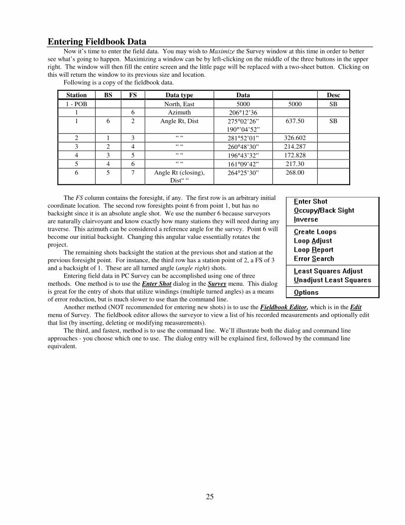
Following is a copy of the fieldbook data.
The FS column contains the foresight, if any. The first row is an arbitrary initial
coordinate location. The second row foresights point 6 from point 1, but has no
backsight since it is an absolute angle shot. We use the number 6 because surveyors
are naturally clairvoyant and know exactly how many stations they will need during any
traverse. This azimuth can be considered a reference angle for the survey. Point 6 will
become our initial backsight. Changing this angular value essentially rotates the
project.
The remaining shots backsight the station at the previous shot and station at the
previous foresight point. For instance, the third row has a station point of 2, a FS of 3
and a backsight of 1. These are all turned angle (angle right) shots.
Entering field data in PC Survey can be accomplished using one of three
methods. One method is to use the Enter Shot dialog in the Survey menu. This dialog
is great for the entry of shots that utilize windings (multiple turned angles) as a means
of error reduction, but is much slower to use than the command line.
Another method (NOT recommended for entering new shots) is to use the Fieldbook Editor, which is in the Edit
menu of Survey. The fieldbook editor allows the surveyor to view a list of his recorded measurements and optionally edit
that list (by inserting, deleting or modifying measurements).
The third, and fastest, method is to use the command line. We’ll illustrate both the dialog and command line
approaches - you choose which one to use. The dialog entry will be explained first, followed by the command line
equivalent.
Station BS FS Data type Data Desc
1 - POB North, East 5000 5000 SB
1 6 Azimuth 206°12’36
1 6 2 Angle Rt, Dist 275°02’26”
190°’04’52”
637.50 SB
2 1 3 “ “ 281°52’01” 326.602
3 2 4 “ “ 260°48’30” 214.287
4 3 5 “ “ 196°43’32” 172.828
5 4 6 “ “ 161°09’42” 217.30
6 5 7 Angle Rt (closing),
Dist“ “ 264°25’30” 268.00

26
1) Select Enter Shot from the Survey
menu (in the Survey window of PC
SURVEY.... isn’t this getting a bit
redundant?). A dialog similar to the
one shown will appear. The first
measurement isn’t really a
measurement at all - it’s a starting
point. Unless you’re working with
GPS and state plane grid coordinates,
you haven’t the foggiest idea of what
the coordinates are, so we’ll pick a
common value of 5000 North and
5000 East. (The units, if you haven’t
noticed, default to US Feet. You also
have the choice of meters and
International Feet). Notice that the
cursor is flashing in the North entry box, the
program having assumed that you wished to start
at point 1. Notice that the Elevation box is
active (i.e. it’s not grayed out). This means that
the dialog is expecting a value for the elevation.
We need to change that.
2) Press the Entry Mode button. A dialog similar
to the one shown on the right will appear.
Notice that just about everything is disabled
(grayed out). This is because we’re in the
North, East entry mode - little else applies.
However, you’ll notice that two possibilities
exist for Elevation Entry.
3) Select None in the Elevation Entry section.
4) Select OK to close this dialog. This will take us
back to the Shot Entry dialog.
5) Enter 5000 for the North value and press
<Enter>.
6) Similarly, enter 5000 for the East value and,
again, press <Enter>. At this point, the cursor
will be flashing in the Description box.
7) Press <Enter> one more time OR press the
Continue button - the result is the same. The
dialog will disappear briefly and will reappear
with empty entry boxes except for the STN Pt,
which is now set to 2. We are now ready to
enter the second measurement.
The first measurement establishes the backsight for
our first point as well as the angular position of another
point in the traverse loop. The REAL orientation is not
known yet, so an angular measurement is made to point 6
(the backsight) at an approximate azimuth of 206°12’36”.
Altering this azimuth later will result in rotating the whole traverse while maintaining angular relationships. Therefore, it
is easy to transform the traverse to whatever orientation is desired after all the data is entered. So, we need to enter an
azimuth but, if we are using the dialog method, it is expecting a coordinate. One way to change the mode is to use the
Entry Mode button.
8) Press the Entry Mode button. This will again bring up the Entry Mode dialog box.
9) Click on the North, East checkbox to so that it is no longer selected. Notice that all the other options now
become active.
27
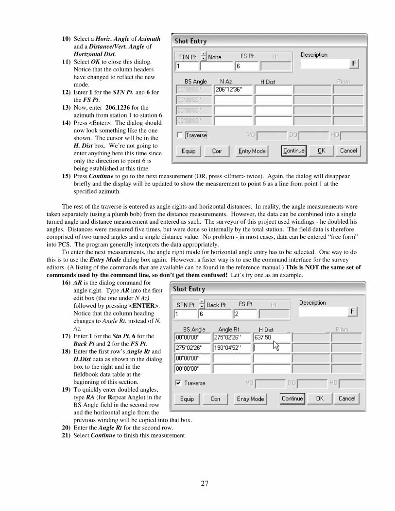
10) Select a Horiz. Angle of Azimuth
and a Distance/Vert. Angle of
Horizontal Dist.
11) Select OK to close this dialog.
Notice that the column headers
have changed to reflect the new
mode.
12) Enter 1 for the STN Pt. and 6 for
the FS Pt.
13) Now, enter 206.1236 for the
azimuth from station 1 to station 6.
14) Press <Enter>. The dialog should
now look something like the one
shown. The cursor will be in the
H. Dist box. We’re not going to
enter anything here this time since
only the direction to point 6 is
being established at this time.
15) Press Continue to go to the next measurement (OR, press <Enter> twice). Again, the dialog will disappear
briefly and the display will be updated to show the measurement to point 6 as a line from point 1 at the
specified azimuth.
The rest of the traverse is entered as angle rights and horizontal distances. In reality, the angle measurements were
taken separately (using a plumb bob) from the distance measurements. However, the data can be combined into a single
turned angle and distance measurement and entered as such. The surveyor of this project used windings - he doubled his
angles. Distances were measured five times, but were done so internally by the total station. The field data is therefore
comprised of two turned angles and a single distance value. No problem - in most cases, data can be entered “free form”
into PCS. The program generally interprets the data appropriately.
To enter the next measurements, the angle right mode for horizontal angle entry has to be selected. One way to do
this is to use the Entry Mode dialog box again. However, a faster way is to use the command interface for the survey
editors. (A listing of the commands that are available can be found in the reference manual.) This is NOT the same set of
commands used by the command line, so don’t get them confused! Let’s try one as an example.
16) AR is the dialog command for
angle right. Type AR into the first
edit box (the one under N Az)
followed by pressing <ENTER>.
Notice that the column heading
changes to Angle Rt. instead of N.
Az.
17) Enter 1 for the Stn Pt, 6 for the
Back Pt and 2 for the FS Pt.
18) Enter the first row’s Angle Rt and
H.Dist data as shown in the dialog
box to the right and in the
fieldbook data table at the
beginning of this section.
19) To quickly enter doubled angles,
type RA (for Repeat Angle) in the
BS Angle field in the second row
and the horizontal angle from the
previous winding will be copied into that box.
20) Enter the Angle Rt for the second row.
21) Select Continue to finish this measurement.

28
22) Continue entering the data from the table until
it is all done. Remember to select OK and NOT
Continue on the last entry. If you select
Continue by mistake, you’ll be faced with
another entry dialog. That’s all right - just
select Cancel to exit data entry. You should
end up with something that looks like this
(ignoring the mapcheck data):

29
The Command Line Approach
Using the command line, as mentioned above, is an alternative way to enter data. The advantage of the command
line is that it is faster because fewer keystrokes are required to enter the same information. It does not offer as much
flexibility as the dialog since it cannot accept windings or repeating angles nor special modes such as Hold Angle, Hold
Side, etc.
To begin the command line approach, type CS 5000 5000 <Enter> or CS 5000,5000 <Enter> from the keyboard.
Notice that the numbers (we call them arguments) can be separated by either a space or a comma. CS is an abbreviation
for Coordinate Store. We’ll abbreviate this command in the following way:
Command: CS 5000 5000 <Enter>
If you remember, the second measurement was a distanceless measurement of point 6 from point 1. The command
line is not capable of entering distanceless measurements, so refer to steps 8-14 in the previous section to enter this
measurement. After the measurement from point 1 to point 6 has been entered, we can use the TRaverse command for the
remaining entries.
The command line for the measurement from point 1 to point 2 looks like the following:
Command: TR 275.0226, 5, 637.50 <Enter>
Much simpler, huh? The first argument of the command, 275.0226, is the horizontal angle. The second argument,
5, controls the interpretation of the horizontal angle value. Quad 0 means that the horizontal angle is an azimuth. Quads 1
through 4 are for bearings, quad 5 is for angle right and quad 6 is for deflection right. If you happen to be entering angle
left or deflection left values, just use negative angle values with the appropriate quad number. The distance (horizontal or
slope), 637.50, is entered after the quad.
A restriction exists in that the command line currently has no way of accepting windings. If you need to enter
winding data, you will have to use the dialogs. If you are using the command line method for this tutorial, use the first
turned angle and ignore the winding.
The command line remembers the last command used so, for the next shots, since you have just used the TR
command, you will not need to enter it again. The previous command can be simply recalled by pressing the
spacebar or by pressing one of the keys on the number pad. If you press the number 5 on the number pad, for
example, the TR command will immediately appear in the status bar followed by the number 5.-Anyway, the commands
are as follows:
TR 281.5201, 326.602 <Enter>
(since you’re still doing angle right, you don’t need to reenter the 5 quad value)
TR 260.4830, 214.287 <Enter>
TR 196.4332, 172.828 <Enter>
TR 161.0942, 217.30 <Enter>
TR 264.2530, 268.00 <Enter>
If you are using the number pad, remember to turn the <Num Lock> on. Pressing the <+ > key will enter the
commas between the numbers. You can therefore do the entire data entry from the number pad once the command for the
first entry has been typed in since pressing any number on the pad will recall the previous command automatically.
Example: 281.5201<+> 326.602 <Enter>

30
This is supposed to be a closed traverse - but something is wrong. The distance between points 1 and 7 is too great.
Hmm... You recheck your data and find that... I LIED! The distance from station 4 to 5 is NOT 172.828. It’s really
supposed to be 122.828. Invoking the Fieldbook Editor at this point is probably a more productive approach than cursing
the author of this heinous crime. As mentioned before, the editor can be used for data entry, but it also is what is used to
alter data that has already been entered.
Invoke the editor by clicking
on Fieldbook Editor in the Edit
menu of Survey.
The upper portion of the
editor contains summary
information on the station point,
backsight point and instrument
height of the current measurement.
The spreadsheet section of the
dialog is the gridded area. The
current measurement is the row
that includes the currently
highlighted field. As the current
row changes, the headings at the
top of the columns may change as
well to reflect the kind of data that
is in each column of the current
row. For instance, selecting the
first row will result in a North and
East column heading since this
first shot was a coordinate store.
Selecting the second row results in
columns labeled N Az and H Dist
since the second shot was an
azimuth and horizontal distance
shot.
Notice that the rows have different shadings. Measurements that comprise the same shot have the same shading -
the shading helps to quickly see the difference between station setups.
The scroll bars on the right and bottom can be used to move around in the spreadsheet when not all the data is
visible. Also notice that when you move the mouse over the edges of the dialog box, the cursor will become the double
arrow cursor. This means that this dialog box can be resized to show more or less data at one time.
Look at row #7. Double-click on the H Dist column of 172.828 and change it to 122.828. Click on OK and the
display will be updated. Notice that the traverse now looks closed. There is a small error, of course, that you can see by
zooming in closely.
Corrected Fieldbook
31
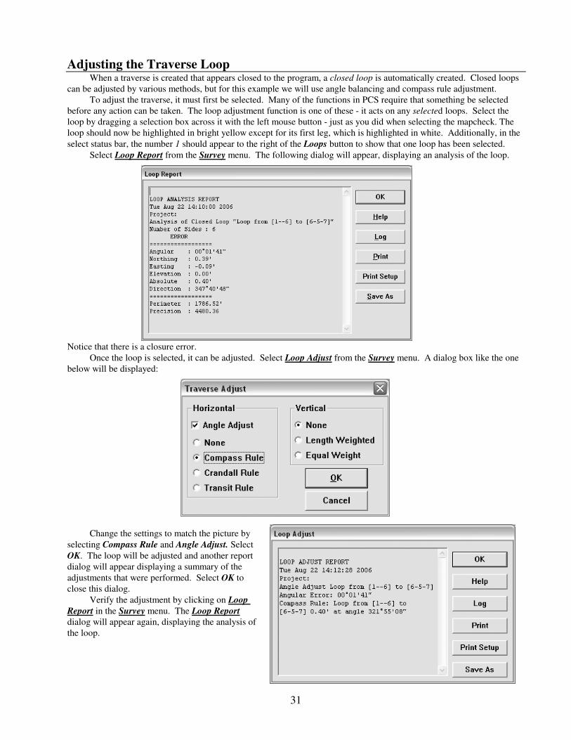
Adjusting the Traverse Loop When a traverse is created that appears closed to the program, a closed loop is automatically created. Closed loops
can be adjusted by various methods, but for this example we will use angle balancing and compass rule adjustment.
To adjust the traverse, it must first be selected. Many of the functions in PCS require that something be selected
before any action can be taken. The loop adjustment function is one of these - it acts on any selected loops. Select the
loop by dragging a selection box across it with the left mouse button - just as you did when selecting the mapcheck. The
loop should now be highlighted in bright yellow except for its first leg, which is highlighted in white. Additionally, in the
select status bar, the number 1 should appear to the right of the Loops button to show that one loop has been selected.
Select Loop Report from the Survey menu. The following dialog will appear, displaying an analysis of the loop.
Notice that there is a closure error.
Once the loop is selected, it can be adjusted. Select Loop Adjust from the Survey menu. A dialog box like the one
below will be displayed:
Change the settings to match the picture by
selecting Compass Rule and Angle Adjust. Select
OK. The loop will be adjusted and another report
dialog will appear displaying a summary of the
adjustments that were performed. Select OK to
close this dialog.
Verify the adjustment by clicking on Loop
Report in the Survey menu. The Loop Report
dialog will appear again, displaying the analysis of
the loop.

32
Generating COGO points Once the traverse loop has been entered
and adjusted, you’ll want to send the point
data over to COGO to allow performing a
stakeout of the property corners from the
traverse station points.
1) Select Generate COGO points from
the Edit menu of Survey.
You should see a dialog box similar to
the one shown. It will list all points and the
shots that create them. It behaves similarly to
the Fieldbook Editor. As the current row
changes, the headings at the top of the
columns may change as well to reflect the kind
of data that is in the each column of the current row. The checkboxes in the first two columns are the only fields that can
be edited. The other fields are provided for reference only.
Notice that the shots that created points 1 and 7 are listed next to each other with the same color. Any points that
are ‘really’ close together will be listed together to show that they can optionally be averaged together to become the same
COGO point. Also, in Survey (but not in COGO), it is possible to have two different points with the same point number,
such as with multiply determined sideshots. These points will also be grouped together in this dialog to show that they can
also become the same COGO point.
After we adjusted our loop, points 1 and 7 (represented in rows 1 and 2 in the above picture) have the same location.
2) We don’t want to transfer both points, we can click in the Use checkbox for row 2 to get rid of the check. Now
point 7 will not be transferred to COGO. Anything that has no check in the Use column will not transfer to
COGO.
If we had left the check, they would have become two different points in COGO.
To change the width of any column, move the mouse to the line in the header row that separates that column from
the next column. The cursor should change to a || with arrows on each side. Click and drag the mouse until the column is
the size you want. You can change the size of the entire dialog by moving the cursor onto the edges or corners, clicking
the left mouse and dragging the edge of the dialog.
To create one COGO point that is an average of both points, click in the Mult column for both rows. This checkbox
is used to show that a COGO point will be created by averaging multiple survey points.
In summary, if Use is not checked, the point will not transfer to COGO. If Use is checked and Multiple is not, the
Survey point will be directly transferred to COGO. If both Use and Multiple are checked, the position will be averaged in
with any other points grouped with this point which are also checked in both columns.
So, for example, if you had four shots to point #22 and three were checked in the Use column and two of those three
were also marked in the Multiple column, these two shots would be averaged to create one COGO point, the shot marked
Use but not Multiple would create another COGO point (with a different COGO point number), and the final shot would
essentially be ignored. When you click OK, the traverse loop points will be transferred to the COGO window.
33
GO to COGO
If you have not purchased the Survey module, open COGO.PCS (in the PCS/TUTORIAL directory) to work through this section.
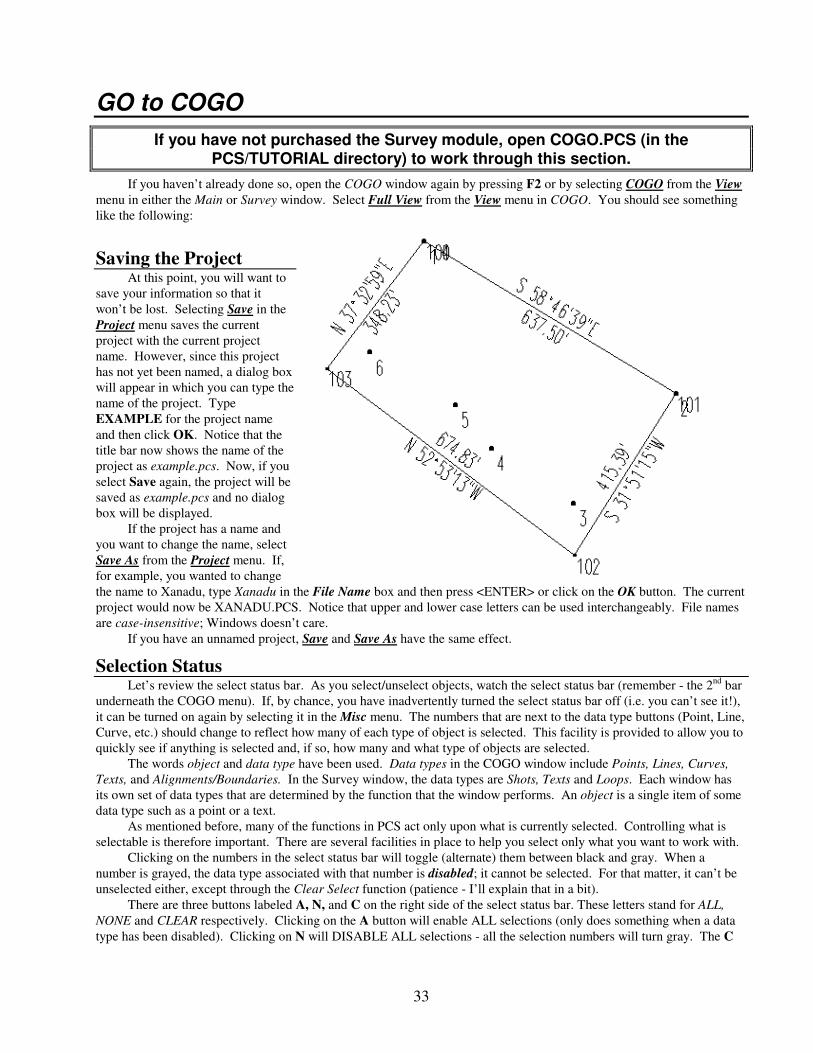
If you haven’t already done so, open the COGO window again by pressing F2 or by selecting COGO from the View
menu in either the Main or Survey window. Select Full View from the View menu in COGO. You should see something
like the following:
Saving the Project At this point, you will want to
save your information so that it
won’t be lost. Selecting Save in the
Project menu saves the current
project with the current project
name. However, since this project
has not yet been named, a dialog box
will appear in which you can type the
name of the project. Type
EXAMPLE for the project name
and then click OK. Notice that the
title bar now shows the name of the
project as example.pcs. Now, if you
select Save again, the project will be
saved as example.pcs and no dialog
box will be displayed.
If the project has a name and
you want to change the name, select
Save As from the Project menu. If,
for example, you wanted to change
the name to Xanadu, type Xanadu in the File Name box and then press <ENTER> or click on the OK button. The current
project would now be XANADU.PCS. Notice that upper and lower case letters can be used interchangeably. File names
are case-insensitive; Windows doesn’t care.
If you have an unnamed project, Save and Save As have the same effect.
Selection Status Let’s review the select status bar. As you select/unselect objects, watch the select status bar (remember - the 2
nd bar
underneath the COGO menu). If, by chance, you have inadvertently turned the select status bar off (i.e. you can’t see it!),
it can be turned on again by selecting it in the Misc menu. The numbers that are next to the data type buttons (Point, Line,
Curve, etc.) should change to reflect how many of each type of object is selected. This facility is provided to allow you to
quickly see if anything is selected and, if so, how many and what type of objects are selected.
The words object and data type have been used. Data types in the COGO window include Points, Lines, Curves,
Texts, and Alignments/Boundaries. In the Survey window, the data types are Shots, Texts and Loops. Each window has
its own set of data types that are determined by the function that the window performs. An object is a single item of some
data type such as a point or a text.
As mentioned before, many of the functions in PCS act only upon what is currently selected. Controlling what is
selectable is therefore important. There are several facilities in place to help you select only what you want to work with.
Clicking on the numbers in the select status bar will toggle (alternate) them between black and gray. When a
number is grayed, the data type associated with that number is disabled; it cannot be selected. For that matter, it can’t be
unselected either, except through the Clear Select function (patience - I’ll explain that in a bit).
There are three buttons labeled A, N, and C on the right side of the select status bar. These letters stand for ALL,
NONE and CLEAR respectively. Clicking on the A button will enable ALL selections (only does something when a data
type has been disabled). Clicking on N will DISABLE ALL selections - all the selection numbers will turn gray. The C

34
button CLEARS all selections. Anything that has been selected becomes unselected, even if its data type has been
disabled (as mentioned above).
Additionally, you can control (or ‘filter’) which data items of
that type can be selected or unselected. If you click on the Points
button, a dialog box will appear in which you can set a range of point
numbers to include or exclude when selecting or unselecting points.
You can also filter your selections by Description and/or Elevation.
Click on Cancel to close the filter.
Suppose you want to only include points that have a description
that starts with the letter A. This can be done by using regular
expressions. For more information, see the section in the Reference
Manual on Regular Expressions.
For this example, let’s turn the point selection status on (black)
and all of the others off (gray). To do this quickly, click on the N
button on the right of the select status bar. All the select numbers
will turn gray. Now click on the number next to the Points button.
The number will turn black to indicate the selecting of points is
enabled. Now draw the box from left to right over the drawing, just
like you did before. This time, only the points will be selected, even
if the box included other things like lines or texts.
Occupying a Point Various functions use the occupy point. The current occupy
point parameters are displayed in the right side of the status bar, so it
is easy to look at any point by simply occupying that point and
looking at the status bar information.
You can occupy any point in the file by moving the mouse near
the point and holding down the right mouse button and then clicking
the left button or, if you have a three button mouse, by clicking the
middle mouse button.
Another way to set the Occupy Point is to select Occupy/Back
Sight from the Cogo menu or click on the Occupy button in the Tools
window. Either of these options will bring up a dialog box (similar
to the one shown). While the dialog box is up, you can either type
the point number in the box or move the mouse near the point in the
data window and click the left button. If you click the mouse a
second time, it will replace the previous value with the next closest
point. When you have the point you want, select the OK button or
press <ENTER>. If you change your mind and do not want to
change the occupy point, click on the Cancel button or type <ESC>.
The command line approach is:
Command: OC Pnt <Enter>
Pnt is the number of the point you wish to occupy.
Points Filter Dialog

35
Deleting Items The data is a bit cluttered. We really don’t need point 101 since it is the same as point 2 or points 100 and 104 since
they are the same as point 1. Let’s clean things up a bit by deleting these points. Deleting, like just about everything else,
uses the select list.
We need to select the points that we want to delete but we need to be careful not to select anything else. A quick
way to select individual items is to do a left-click and release (NO DRAG!) in the vicinity of the desired object. This will
select the nearest item. Performing another left-click and release will unselect the first item and select the nearest item -
and so on and so forth.
For this example, though, we’re going to use a more elaborate approach to give you an idea of the control that can
be exerted in selecting objects.
•• Click on the C button in the select status bar to make sure that nothing is selected.
•• Click on the N button to turn off the selectability of all data types.
•• Click on the number next to the Pts button to enable selecting points.
Now points are the only data type that can be selected.
In addition, let’s click on the Pts button to set up the point filter. Click on the Point Numbers checkbox so that
point number filtering is enabled. Make sure that Include for point numbers is selected and then type 100-110 in the
Point Number edit box. This will only allow selecting points with numbers from 100 to 110. Click on the OK button.
We will still need to be careful not to select points 102 and 103. Draw a selection box around point 100 and 104
then draw another selection box around point 101. The selection status bar should show 3 points selected. Now, go to the
Edit menu and select Delete Objects. A dialog box will pop up
showing the number of items selected and asking if you want to
continue. The program, concerned for your welfare, just wants to
make sure that you do not delete anything by accident. Of course,
there is always the Undo function. So you can be brave and click
Yes. Now don’t panic when you see that some lines and texts were
also deleted. When you delete a point, any lines or curves that
were connected to it will be deleted. When a line is deleted, any
text on the line like the bearing and distance text will also be
deleted.
Open the Pts filter again and turn off the Point Numbers
filtering before continuing.
As I said, this is a much more involved procedure than we needed, but you should now have a better appreciation for
the control that is available if needed.
Connect Points Now we will want to create the
boundary of the lot using points 1, 2,
102, and 103. To do this, select
Connect Points from the Cogo menu or
click on the Connect Points button
(shown above). Since we still have the line from 102 to 103,
we will just traverse from 103 to 1 to 2 to 102. So set the
Occupy Pt, which is the starting point for the traverse to 103.
We could just type one point number at a time in the Point
Number box clicking Continue each time but we can also
enter the whole series of points at once as 1-2, 102. This means use every point from 1 to 2 and then use 102. If we click
OK, the points will be connected in order and we now have our boundary.
The command for Connect Points is: PT Pnt List. The first point in Pnt List corresponds to the Occupy Pt in the
dialog. Therefore, to perform this same function, we can type:
Command: PT 103, 1-2, 102<Enter> or
PT 103,1,2,102<Enter>
Connect Points
button

36
Creating a Boundary In PC Survey, a series of connected lines and curves is called a boundary or alignment. Boundaries start and end at
about the same point. Boundaries have a name, an area and perimeter. They are easily annotated with any combination of
these values (name, area, perimeter), so they are very useful for representing property lots. Alignments don’t start and end
at about the same location - they can be used for road centerlines. Alignments and boundaries can be automatically
created during traversing but this option is off by default. Functions that use alignments and boundaries include
Predetermined Area, Offset, and Bnd/Aln-Annotation. To create a boundary from existing bounding lines and/or curves,
the lines and/or curves that bound the area which is to be enclosed by the boundary must first be selected. We want to
create a boundary of the lines bounding the property so that the Predetermined Area functions can be used to subdivide
the lot.
Making sure lines are selectable, select the four bounding lines of the property that we just created. The four lines
should now be highlighted in bright red (assuming you haven’t changed the color definitions).
Now, to create a boundary of these lines, select Create from the Bnd menu. PC Survey will display a message
showing that one boundary was created. It will also automatically select the boundary. This is convenient for us since, to
look at the area and perimeter information, the boundary needs to be selected. If you want to select an alignment or
boundary, the selection box only needs to intersect one of the lines/curves in the alignment/boundary. When a boundary is
selected, it is highlighted by being filled with cross-hatched lines. When an alignment is selected, it is highlighted with a
heavy yellow line. In both cases, the first half of the first line in the alignment/boundary is highlighted in white.
Computing Area
Example of Boundary highlighting

37
At this point, the number of selected alignments/boundaries should be 1. Select Info from the Bnd menu. This will
bring up a dialog box that will list all selected alignments/boundaries (we only have one in this case) with their associated
perimeter and area (in both acres and square feet). The totals will be displayed in the bottom of the box. Since we have
not named this boundary yet, the program gave it a name of Lot 1 and we can see that the lot encloses 5.74 acres and has a
perimeter of 2075.77 feet.
Alignment/Boundary Info Dialog
If we want to name this boundary “Lot A”, click on the Rename button, which will bring up a dialog box. Type in
Lot A followed by pressing <ENTER> or clicking on the OK button. After this dialog box disappears, notice that the
name of the boundary as listed in the Info box is now Lot A. When you are tired of this dialog box, click Close to move
on.
Subdividing the Lot - Predetermined Area We’re now ready to subdivide the property by
dividing it into three equally sized lots with division
lines that are perpendicular to the frontage line.
There are two predetermined area functions. One
uses the sliding line method (By sliding line) and the
other is a hinged method (By pivot line). The sliding
line method is applicable to this problem.
1) With the boundary selected, select
Predetermined Area - By sliding line
from the Bnd menu. A dialog box similar
to the one shown will appear.
This is going to be a two-step process. We
will first cut off a parcel that is one-third of the total
size. Then we will split the remaining two-thirds in
half. We could continue the process, by splitting the
half in half again, but that could be fattening since
that would get us Half & Half.
The Area shown in the dialog is the current
area of the property. The value of 5.74 is the acreage
of the area to 2 decimal places of precision. This is
not a lot of precision, so click on the Sq. Feet radio
button to change the value to square feet
(249820.05). Since there are many more significant
digits in this value, when we divide by 3, the internal
result will be more accurate. Since we want to divide
the lot into three sections, append /3 to the end of the
area value so the Area now reads 249820.05/3.
2) For Direction of Cutting Line, click on Select Line, which shows that we will be defining the direction of the
cutting line by using a line that already exists.
Predetermined Area by Sliding Line dialog
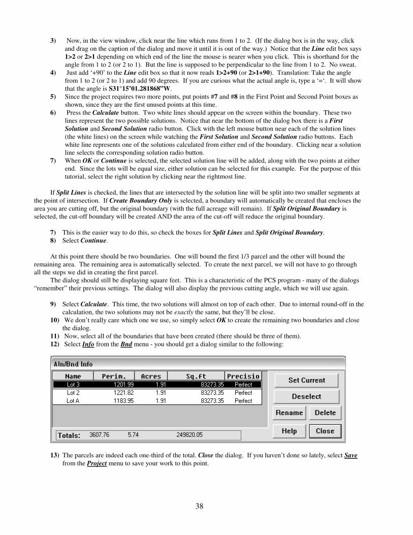
38
3) Now, in the view window, click near the line which runs from 1 to 2. (If the dialog box is in the way, click
and drag on the caption of the dialog and move it until it is out of the way.) Notice that the Line edit box says
1>2 or 2>1 depending on which end of the line the mouse is nearer when you click. This is shorthand for the
angle from 1 to 2 (or 2 to 1). But the line is supposed to be perpendicular to the line from 1 to 2. No sweat.
4) Just add ‘+90’ to the Line edit box so that it now reads 1>2+90 (or 2>1+90). Translation: Take the angle
from 1 to 2 (or 2 to 1) and add 90 degrees. If you are curious what the actual angle is, type a ‘=‘. It will show
that the angle is S31°15’01.281868”W.
5) Since the project requires two more points, put points #7 and #8 in the First Point and Second Point boxes as
shown, since they are the first unused points at this time.
6) Press the Calculate button. Two white lines should appear on the screen within the boundary. These two
lines represent the two possible solutions. Notice that near the bottom of the dialog box there is a First
Solution and Second Solution radio button. Click with the left mouse button near each of the solution lines
(the white lines) on the screen while watching the First Solution and Second Solution radio buttons. Each
white line represents one of the solutions calculated from either end of the boundary. Clicking near a solution
line selects the corresponding solution radio button.
7) When OK or Continue is selected, the selected solution line will be added, along with the two points at either
end. Since the lots will be equal size, either solution can be selected for this example. For the purpose of this
tutorial, select the right solution by clicking near the rightmost line.
If Split Lines is checked, the lines that are intersected by the solution line will be split into two smaller segments at
the point of intersection. If Create Boundary Only is selected, a boundary will automatically be created that encloses the
area you are cutting off, but the original boundary (with the full acreage will remain). If Split Original Boundary is
selected, the cut-off boundary will be created AND the area of the cut-off will reduce the original boundary.
7) This is the easier way to do this, so check the boxes for Split Lines and Split Original Boundary.
8) Select Continue.
At this point there should be two boundaries. One will bound the first 1/3 parcel and the other will bound the
remaining area. The remaining area is automatically selected. To create the next parcel, we will not have to go through
all the steps we did in creating the first parcel.
The dialog should still be displaying square feet. This is a characteristic of the PCS program - many of the dialogs
“remember” their previous settings. The dialog will also display the previous cutting angle, which we will use again.
9) Select Calculate. This time, the two solutions will almost on top of each other. Due to internal round-off in the
calculation, the two solutions may not be exactly the same, but they’ll be close.
10) We don’t really care which one we use, so simply select OK to create the remaining two boundaries and close
the dialog.
11) Now, select all of the boundaries that have been created (there should be three of them).
12) Select Info from the Bnd menu - you should get a dialog similar to the following:
13) The parcels are indeed each one-third of the total. Close the dialog. If you haven’t done so lately, select Save
from the Project menu to save your work to this point.
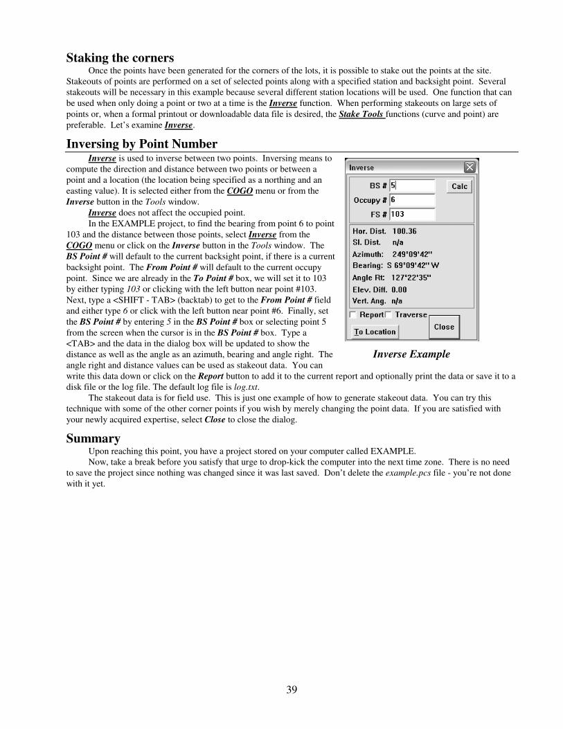
39
Staking the corners Once the points have been generated for the corners of the lots, it is possible to stake out the points at the site.
Stakeouts of points are performed on a set of selected points along with a specified station and backsight point. Several
stakeouts will be necessary in this example because several different station locations will be used. One function that can
be used when only doing a point or two at a time is the Inverse function. When performing stakeouts on large sets of
points or, when a formal printout or downloadable data file is desired, the Stake Tools functions (curve and point) are
preferable. Let’s examine Inverse.
Inversing by Point Number Inverse is used to inverse between two points. Inversing means to
compute the direction and distance between two points or between a
point and a location (the location being specified as a northing and an
easting value). It is selected either from the COGO menu or from the
Inverse button in the Tools window.
Inverse does not affect the occupied point.
In the EXAMPLE project, to find the bearing from point 6 to point
103 and the distance between those points, select Inverse from the
COGO menu or click on the Inverse button in the Tools window. The
BS Point # will default to the current backsight point, if there is a current
backsight point. The From Point # will default to the current occupy
point. Since we are already in the To Point # box, we will set it to 103
by either typing 103 or clicking with the left button near point #103.
Next, type a <SHIFT - TAB> (backtab) to get to the From Point # field
and either type 6 or click with the left button near point #6. Finally, set
the BS Point # by entering 5 in the BS Point # box or selecting point 5
from the screen when the cursor is in the BS Point # box. Type a
<TAB> and the data in the dialog box will be updated to show the
distance as well as the angle as an azimuth, bearing and angle right. The
angle right and distance values can be used as stakeout data. You can
write this data down or click on the Report button to add it to the current report and optionally print the data or save it to a
disk file or the log file. The default log file is log.txt.
The stakeout data is for field use. This is just one example of how to generate stakeout data. You can try this
technique with some of the other corner points if you wish by merely changing the point data. If you are satisfied with
your newly acquired expertise, select Close to close the dialog.
Summary Upon reaching this point, you have a project stored on your computer called EXAMPLE.
Now, take a break before you satisfy that urge to drop-kick the computer into the next time zone. There is no need
to save the project since nothing was changed since it was last saved. Don’t delete the example.pcs file - you’re not done
with it yet.
Inverse Example

40
More COGO As described earlier, the customer has a development plan for the piece of property you have stored as the project
file named example.pcs. The first step in that plan involved subdividing the property into three lots. With the three lots
divided, we’ll now have to find something to do to exercise some of the other functions in the program. Okay, let’s say
the owner has decided to build a strategic missile silo. The silo entrance will have a covered entrance that houses a
vehicle elevator so that he can store his Abrams M1 main battle tank and ‘71 Volkswagon SuperBeetle 300’ underground.
Being an intelligent person, the owner recognizes that it is only a matter of time before one of the Russian wheat
farmers would try to hook one of those ICBMs left lying around to his plow. Of course, farmer Boris could easily screw
up the launch programming and the owner intends to reply in kind if such an event throws a MIRVed warhead in HIS
direction.
Given this common scenario, we need to place a silo entrance and steel-reinforced driveway from the entrance to the
street (those M1s are HEAVY). We’ll worry about the silo blast doors and early warning radar placement later (if Boris
doesn’t send a present our way first).
The silo architect visits the property to pick out a good location for the entrance. He stakes out the corners of the
proposed building and your crew chief takes a few shots to locate the building on the plat. However, this time he decides
to use his trusty GollyWhomper 2000 data collector (the .44 Magnum model) to reduce the data down to a set of
coordinates. He does this, of course, because he knows that we needed an example of how to import points from an
ASCII file.
Importing an ASCII point file This point file is called SILO.ASC and is found in your TUTORIAL directory. To import this data, select Import
� Points from…�File from the Project menu. The following dialog will appear:
Well - something LIKE this dialog will appear. After you go up one folder, then open the TUTORIAL directory,
and then select the SILO.ASC file it will look more like the above. Notice the Format section on the bottom left. This is
where you specify what kind of file it is that you are trying to import. In this case we are importing a Delim Ascii file that
has the PNE format (Point number, Northing and Easting). The Filter button is used for restricting what points are to be
imported from the specified file. In our case, we want ‘em all, so there is no need to fool with the Filter settings. This
dialog is a derivative of the standard Windows file dialog. If you are totally lost as to how to use this kind of dialog to
locate a file, review your Windows documentation to get a basic understanding of how Windows works.
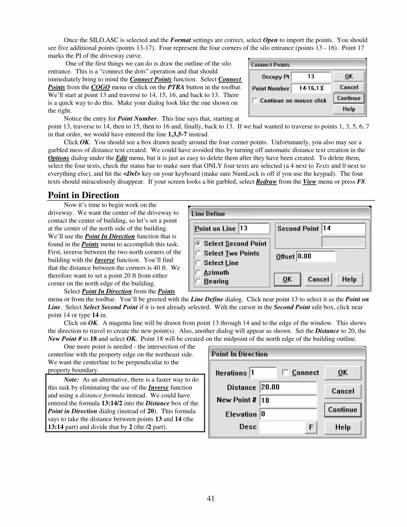
41
Once the SILO.ASC is selected and the Format settings are correct, select Open to import the points. You should
see five additional points (points 13-17). Four represent the four corners of the silo entrance (points 13 - 16). Point 17
marks the PI of the driveway curve.
One of the first things we can do is draw the outline of the silo
entrance. This is a “connect the dots” operation and that should
immediately bring to mind the Connect Points function. Select Connect
Points from the COGO menu or click on the PTRA button in the toolbar.
We’ll start at point 13 and traverse to 14, 15, 16, and back to 13. There
is a quick way to do this. Make your dialog look like the one shown on
the right.
Notice the entry for Point Number. This line says that, starting at
point 13, traverse to 14, then to 15, then to 16 and, finally, back to 13. If we had wanted to traverse to points 1, 3, 5, 6, 7
in that order, we would have entered the line 1,3,5-7 instead.
Click OK. You should see a box drawn neatly around the four corner points. Unfortunately, you also may see a
garbled mess of distance text created. We could have avoided this by turning off automatic distance text creation in the
Options dialog under the Edit menu, but it is just as easy to delete them after they have been created. To delete them,
select the four texts, check the status bar to make sure that ONLY four texts are selected (a 4 next to Texts and 0 next to
everything else), and hit the <Del> key on your keyboard (make sure NumLock is off if you use the keypad). The four
texts should miraculously disappear. If your screen looks a bit garbled, select Redraw from the View menu or press F8.
Point in Direction Now it’s time to begin work on the
driveway. We want the center of the driveway to
contact the center of building, so let’s set a point
at the center of the north side of the building.
We’ll use the Point In Direction function that is
found in the Points menu to accomplish this task.
First, inverse between the two north corners of the
building with the Inverse function. You’ll find
that the distance between the corners is 40 ft. We
therefore want to set a point 20 ft from either
corner on the north edge of the building.
Select Point In Direction from the Points
menu or from the toolbar. You’ll be greeted with the Line Define dialog. Click near point 13 to select it as the Point on
Line. Select Select Second Point if it is not already selected. With the cursor in the Second Point edit box, click near
point 14 or type 14 in.
Click on OK. A magenta line will be drawn from point 13 through 14 and to the edge of the window. This shows
the direction to travel to create the new point(s). Also, another dialog will appear as shown. Set the Distance to 20, the
New Point # to 18 and select OK. Point 18 will be created on the midpoint of the north edge of the building outline.
One more point is needed - the intersection of the
centerline with the property edge on the northeast side.
We want the centerline to be perpendicular to the
property boundary.
Note: As an alternative, there is a faster way to do
this task by eliminating the use of the Inverse function
and using a distance formula instead. We could have
entered the formula 13:14/2 into the Distance box of the
Point in Direction dialog (instead of 20). This formula
says to take the distance between points 13 and 14 (the
13:14 part) and divide that by 2 (the /2 part).

42
Bearing-Bearing Intersection
To get this point, use the Bearing-Bearing
intersection routine in the Intsct menu. This routine
essentially finds the intersection of two lines and
therefore uses the Line Define dialog box twice. After
selecting this function, fill in the first Line Define dialog
to look like the one on the right.
In this dialog, we are defining our first line to pass
through point 17 with a direction that is perpendicular to
the property line. This dialog behaves very much like the
one we used in Predetermined Area. With Select Line
selected, we can click near the line that we will use for a
reference which in this case is the line from 1 to 10 so the
dialog box will show ‘1>10’. But, since we want the line to be perpendicular to this line, we will subtract 90. If you are
curious what the azimuth would be, type a ‘=‘ and you should see 31°15’01”. You can leave it showing the actual azimuth
or you can type ‘=‘ again to show the formula. Click OK. A magenta line will be drawn on the screen to represent the line
you just defined. It should pass through point 17
and be perpendicular to the northeast edge.
The second Line Define dialog will appear.
We want to define the second line to be colinear (on
top of) the northeast property line. This can be done
in a number of ways. In the method shown, we
define a line that passes through one of the corners
(point 1) and also passes through point 10 using
Select Second Point. Alternatively, you could
select Select Line instead of Select Second Point
and selected the northeast property line with the
mouse. Or you could select Select Two Points and
selected 1 and 10 to define the line Once you have the dialog box filled in, click OK. A second line will be drawn on top
of the northeast property line. The intersection of the two lines will be where the new point will be located.
The third and final dialog for this function will appear
which is used for actually creating the point at the
intersection. You can change the point number and
description that will be assigned to the intersection point by
filling in the appropriate edit boxes. Notice that the distances
from points 1 and 17 to the intersection point are also shown
for additional information. Select OK to create point 19.
The command line syntax for Bearing-Bearing
intersection is: BB Pnt, Angle, Pnt, Angle. To use the
command line, you would then type in
Command: BB 1, 1>10, 17, 1>10-90<Enter>
Notice that you CAN use formulas in the command line.
Now, you’ll want to draw the centerline of the driveway by using Connect Points to draw a line from point 18 to 17
and from point 17 to 19. Remember that Point Traverse is found in the COGO menu. Since you’ve used this function
before, I’m going to leave out the details of this step - you’re on your own. When done you should have a drawing that
looks something like the following:
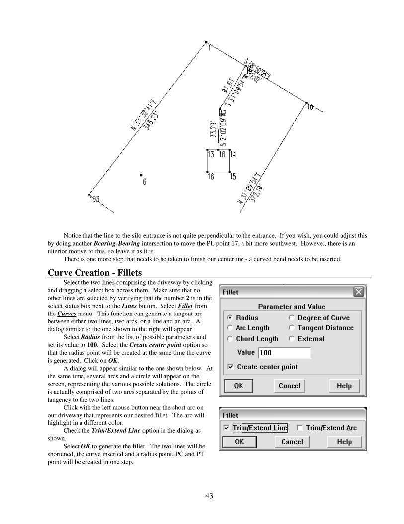
43
Notice that the line to the silo entrance is not quite perpendicular to the entrance. If you wish, you could adjust this
by doing another Bearing-Bearing intersection to move the PI, point 17, a bit more southwest. However, there is an
ulterior motive to this, so leave it as it is.
There is one more step that needs to be taken to finish our centerline - a curved bend needs to be inserted.
Curve Creation - Fillets Select the two lines comprising the driveway by clicking
and dragging a select box across them. Make sure that no
other lines are selected by verifying that the number 2 is in the
select status box next to the Lines button. Select Fillet from
the Curves menu. This function can generate a tangent arc
between either two lines, two arcs, or a line and an arc. A
dialog similar to the one shown to the right will appear
Select Radius from the list of possible parameters and
set its value to 100. Select the Create center point option so
that the radius point will be created at the same time the curve
is generated. Click on OK.
A dialog will appear similar to the one shown below. At
the same time, several arcs and a circle will appear on the
screen, representing the various possible solutions. The circle
is actually comprised of two arcs separated by the points of
tangency to the two lines.
Click with the left mouse button near the short arc on
our driveway that represents our desired fillet. The arc will
highlight in a different color.
Check the Trim/Extend Line option in the dialog as
shown.
Select OK to generate the fillet. The two lines will be
shortened, the curve inserted and a radius point, PC and PT
point will be created in one step.
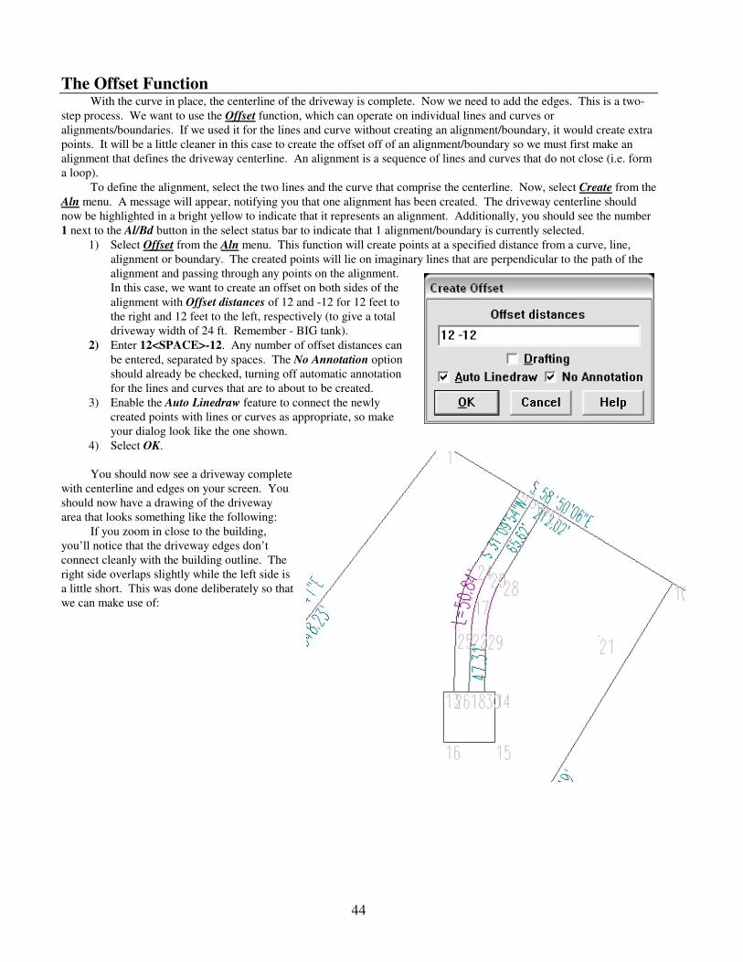
44
The Offset Function With the curve in place, the centerline of the driveway is complete. Now we need to add the edges. This is a two-
step process. We want to use the Offset function, which can operate on individual lines and curves or
alignments/boundaries. If we used it for the lines and curve without creating an alignment/boundary, it would create extra
points. It will be a little cleaner in this case to create the offset off of an alignment/boundary so we must first make an
alignment that defines the driveway centerline. An alignment is a sequence of lines and curves that do not close (i.e. form
a loop).
To define the alignment, select the two lines and the curve that comprise the centerline. Now, select Create from the
Aln menu. A message will appear, notifying you that one alignment has been created. The driveway centerline should
now be highlighted in a bright yellow to indicate that it represents an alignment. Additionally, you should see the number
1 next to the Al/Bd button in the select status bar to indicate that 1 alignment/boundary is currently selected.
1) Select Offset from the Aln menu. This function will create points at a specified distance from a curve, line,
alignment or boundary. The created points will lie on imaginary lines that are perpendicular to the path of the
alignment and passing through any points on the alignment.
In this case, we want to create an offset on both sides of the
alignment with Offset distances of 12 and -12 for 12 feet to
the right and 12 feet to the left, respectively (to give a total
driveway width of 24 ft. Remember - BIG tank).
2) Enter 12<SPACE>-12. Any number of offset distances can
be entered, separated by spaces. The No Annotation option
should already be checked, turning off automatic annotation
for the lines and curves that are to about to be created.
3) Enable the Auto Linedraw feature to connect the newly
created points with lines or curves as appropriate, so make
your dialog look like the one shown.
4) Select OK.
You should now see a driveway complete
with centerline and edges on your screen. You
should now have a drawing of the driveway
area that looks something like the following:
If you zoom in close to the building,
you’ll notice that the driveway edges don’t
connect cleanly with the building outline. The
right side overlaps slightly while the left side is
a little short. This was done deliberately so that
we can make use of:

45
Line Extend The Line Extend function operates on selected lines (no big surprise, here). All selected lines are extended (or
shortened) to contact a chosen line or curve. If a point is chosen as the object to extend to, the selected lines are extended
or shortened until their endpoints lie on a line perpendicular to the endpoint’s line and passing through the chosen point.
The chosen point then becomes a perpendicular offset to the endpoint of each selected line.
1) With all selections cleared, select the two
driveway edges (created in the previous step)
next to the silo entrance.
2) Select Line Extend from the Edit menu. The
highlighting for the two lines will be removed.
A dialog similar to this one will appear:
3) While this dialog is up, select the north side of
the silo (using a select box), which is the line we want to extend the other points to.
Extend endpoint(s) means to change the lines by extending the appropriate endpoint to sit on the selected line.
Create point(s) at intersection means to leave the current line the same but create a new point and a new line from the
current endpoint to the new point. If neither is selected, a new line will be created from the current endpoint to the spot on
the line where the new point would go.
4) In this case, check Extend endpoints(s) since we want to actually alter the lines rather than add a new line to
extend the old one.
5) Click OK and the points should now be sitting at the intersection of the edges of the driveway and the north side
of the silo.
Text Let’s label the road that passes in front of the lot as Birkdale Rd. To do this, we will enter text mode by either
selecting Text from the Draw menu or clicking on the button with the A. The cursor will change to an I-beam to remind
you that we are in text mode. Now, move the cursor to where you want the text to be and click with the left button. A
horizontal bar will appear to show the text insertion point. Now type Birkdale Rd. After this has been done, you have
several options.
•• To add a second line of text, press the <Enter> key to move the insertion point beneath the B.
•• To add another text, move the cursor and click somewhere else and then start typing in the text.
•• To leave text mode, hit the <Esc> key or click again on the A button. The cursor will return to normal.
This is all the text that we want to create for now, so hit the <Esc> key or click on the A button.
The text was placed horizontal to the screen but of course it would look a lot better if it ran parallel to the frontage
line. No problem. Just place the cursor over the text and, holding down the Shift key, click with the right button. (First
make sure that texts are selectable. The text itself doesn’t have to be selected but texts must be selectable. This
makes it easier to select the data type that
you want since some data types make it
difficult to select others.) A popup menu
will appear. Select Align. Boy, this dialog looks a
lot like the Line Define dialog. It works just the
same. Click on Select Line and then click on the
frontage line. The edit box should show a ‘1>10’.
Click OK. The text now heads in the same
direction as the line.
It would look a lot better if the text were
larger so select the text and then select Set Font-
Other from the Edit menu. Let’s make the Size 0.5” tall and set the Font to Roman.
This is one of the strengths of Windows. Any font you have installed in your
Windows can be used by PC Survey. If you haven’t yet done so, close this dialog
by clicking OK. Now Birkdale Rd is much larger and a little fancier.
That’s enough COGO for now. And now for something entirely different.
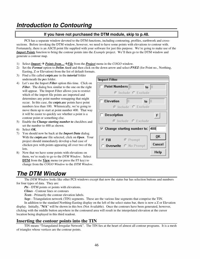
46
Introduction to Contouring
If you have not purchased the DTM module, skip to p.48.
PCS has a separate window devoted to the DTM functions, including contouring, profiles, earthwork and cross-
sections. Before invoking the DTM window, however, we need to have some points with elevations to contour with.
Fortunately, there is an ASCII point file supplied with your software for just this purpose. We’re going to make use of the
Import Points function to bring the contour points into the Example project. We’ll then go to the DTM window and
generate a contour map.
1) Select Import � Points from…�File from the Project menu in the COGO window.
2) Set the Format option to Delim Ascii and then click on the down arrow and select PNEZ (for Point no., Northing,
Easting, Z or Elevation) from the list of default formats.
3) Find a file called cntpts.asc in the tutorial folder
underneath the pcs folder.
4) Let’s use the Import Filter option this time. Click on
Filter. The dialog box similar to the one on the right
will appear. The Import Filter allows you to restrict
which of the import file points are imported and
determines any point number remapping that might
occur. In this case, the cntpts.asc points have point
numbers less than 100. Whimsically, we’re going to
move them up to start at point number 400. That way
it will be easier to quickly see whether a point is a
contour point or something else.
5) Enable the Change starting number to checkbox and
set the number to 400 as shown.
6) Select OK.
7) You should now be back at the Import Data dialog.
With the cntpts.asc file selected, click on Open. Your
project should immediately develop a bad case of
chicken pox with points appearing all over two of the
lots.
8) Now that we have some points with elevations on
them, we’re ready to go to the DTM Window. Select
DTM from the View menu (or press the F5 key) to
change from the COGO Window to the DTM Window.
The DTM Window The DTM Window looks like other PCS windows except that now the status bar has selection buttons and numbers
for four types of data. They are:
Pts - DTM points or points with elevations.
Clines - Contour lines or contours
Texts - Primarily the contour elevation labels.
Segs - Triangulation network (TIN) segments. These are the various line segments that comprise the TIN.
In addition to the standard Northing-Easting display on the left of the select status bar, there is now a Z or Elevation
display. Initially, ”N/A” will be shown in this box (Not Available). Once the contours have been generated, however,
clicking with the middle button anywhere in the contoured area will result in the interpolated elevation at the cursor
location being displayed in this third readout.
Inserting the contour points into the TIN TIN means “Triangulated Irregular Network”. The TIN lies at the heart of almost all contour programs. It is a mesh
of triangles whose vertices are the contour points.
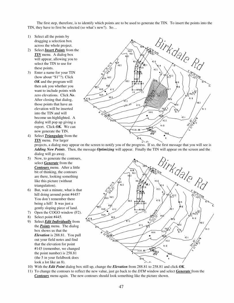
47
The first step, therefore, is to identify which points are to be used to generate the TIN. To insert the points into the
TIN, they have to first be selected (so what’s new?). So…
1) Select all the points by
dragging a selection box
across the whole project.
2) Select Insert Points from the
TIN menu. A dialog box
will appear, allowing you to
select the TIN to use for
these points.
3) Enter a name for your TIN
(how about “S1”?). Click
OK and the program will
then ask you whether you
want to include points with
zero elevations. Click No.
After closing that dialog,
those points that have an
elevation will be inserted
into the TIN and will
become un-highlighted. A
dialog will pop up giving a
report. Click OK. We can
now generate the TIN.
4) Select Triangulate from the
TIN menu. For larger
projects, a dialog may appear on the screen to notify you of the progress. If so, the first message that you will see is
Adding New Points. Then, the message Optimizing will appear. Finally the TIN will appear on the screen and the
dialog will go away.
5) Now, to generate the contours,
select Generate from the
Contours menu. After a little
bit of thinking, the contours
are there, looking something
like this picture (without
triangulation).
6) But, wait a minute, what is that
hill doing around point #445?
You don’t remember there
being a hill! It was just a
gently sloping piece of land.
7) Open the COGO window (F2).
8) Select point #445.
9) Select Edit Individually from
the Points menu. The dialog
box shows us that the
Elevation is 288.81. You pull
out your field notes and find
that the elevation for point
#145 (remember, we changed
the point number) is 258.81
(the 5 in your fieldbook does
look a lot like an 8).
10) With the Edit Point dialog box still up, change the Elevation from 288.81 to 258.81 and click OK.
11) To change the contours to reflect the new value, just go back to the DTM window and select Generate from the
Contours menu again. The new contours should look something like the picture shown.

48
The Layout Window
If you have not purchased the DTM module, open LAYOUT.PCS in the
PCS\TUTORIAL directory to continue the tutorial from this point.
It’s time to make use of another tool of PCS - the Layout Window. The Layout Window is used for arranging your
data on a sheet in preparation for plotting. Open the Layout Window by selecting Layout from the View menu.
The appearance of
this window is similar to
the other windows of PCS.
There is a select status bar
beneath the window’s
menu and a toolbar on the
left side. The left column
toolbar functions are:
Open, Save,
Grid/Snapping, Line
Style, Color, Font, Profile
and Table. The right
column toolbar functions,
from top to bottom, are:
Selection Cursor, Move,
Rotate, 2 point circle, 3
point circle, Arc, Ellipse,
Rectangle,
Polygon/Polyline, Text,
Line, Dimension-Bent,
and Dimension - Curved.
There is also an X-Y
readout in the select status
bar on the left side that
displays page coordinates
as the cursor is moved.
There is a picture of
a sheet of paper in the
center of the paper. The box that is drawn inside the sheet is offset from the edges of the sheet by the margin values set in
the Project | Page Layout settings. This interior box is for reference purposes only and, like the sheet outline, is not
printed. The sheet is initially set to the size and orientation used by the default printer. The default printer is set in the
Printers section of the Windows Control Panel.
This window also includes rulers on the top and left sides that aid in understanding the physical dimensions of the
drawing.
There are four different basic data types in Layout that are referenced by the select status buttons.
Data - Data refers to what you see in the COGO/DTM windows. You can place the entire project (Full View), just
what you see at whatever zoom you’re currently using in the COGO window (Screen View), or use one of the View Areas.
(View Areas haven’t been explained yet - see the reference manual for more information).
Components - Examples of components are title blocks, certifications, north arrows and scales. Components can be
placed in libraries for future use. A sample library named PCS.GLB is included with your software.
Texts - Text is .. text.
Graphics - Examples of graphics are circles, lines, arcs, etc. These are primitive drawing objects. Components are
comprised of a collection of graphics.

49
Setting the sheet size As mentioned, the sheet size that is initially displayed is set to your default printer sheet values.
1) Select Page Layout from the Project menu. This dialog allows you to change the sheet size, margins and sheet
orientation. It also allows you to specify that you are creating more than one page, either for multiple views or for
one view that spans multiple pages. It also allows creating an automatic border at the margins and specifying a
specific line type for the border.
Page Layout Dialog
2) Select Arch D for the Paper Size. Select Landscape for the Orientation.
3) Select OK to close the dialog. If these settings are different from what you originally had, the paper outline in the
Layout Window will change to reflect the new settings.
Placing the data on the sheet Next, you’ll want to place your COGO drawing on the sheet. The COGO data doesn’t look ”finished” yet, but it
doesn’t matter. After you place the COGO drawing in Layout, any changes you make in COGO will be reflected in
Layout.
1) Select Place Full View from the Data menu. The cursor will change to an X-ed out box with a small set of crosshairs
in the upper left. The crosshairs represent the upper left corner of the COGO view data.
2) Move the cursor so that the crosshairs are somewhere in the upper left area of the sheet. Click with the left button.
The COGO data will appear on the sheet.
You probably aren’t going to be satisfied with where the data has been placed. No problem - you can move and
rotate the data to any position and orientation you desire. Its initial orientation is the same as that of COGO. To move or
rotate the data, it must first be selected. However, there is a small problem - the data is not selectable yet. If you look at
the select status bar, you’ll notice that the Data number has been grayed (not selectable) while all the other data types are
black (selectable). This is the default in Layout. The reason for this is that it is too easy to inadvertently select and move
the data view while operating on other items when Data defaults to selectable.

50
Moving objects in Layout 1) Left-click on the Data number to toggle it to black.
2) Select the data view by either single-clicking inside it or
dragging a selection box across it with the left button.
Once selected, an outline box will be drawn around the data
view. The box has nibs on it - little boxes on the corners and on
centers of each of the lines. You can click and drag the nibs to
change the size of the outline box. The only purpose in doing so is if
you wish to clip the drawing. Clipping means to cut off a portion. If
the outline box is shrunk so that only a portion of the drawing is
shown, only that portion will print.
We’re not interested in clipping the drawing right now. We
want to move it so that it has a good position on the sheet. To move
the drawing,
3) Left-click inside the outline box. Keep the button depressed and don’t move the mouse until the data disappears
and all that is left is the outline box.
4) Keep the mouse button depressed and drag the outline box to whatever position suits you.
This move technique - click, hold and drag - is used for moving anything inside the Layout Window. If your mouse
is the type that rolls around (as opposed to a stationary or trackball mouse), you must be careful not to move the mouse
during the slight delay between the initial click and the point where “move mode” has been entered. If the mouse moves
too much too soon, the program will think that you are trying to select something instead of move something.
5) Finally, return the data view to its original un-selectable state by clicking on the C button in the select status bar (far
right side). This will also clear all selections (just like in COGO).
Add a border Now that the data is on the sheet, let’s dress up the sheet a little bit. The first thing that we can do is to add a border.
1) Select the Page Layout command again in the Layout Project menu.
2) Check Draw Border.
3) Think it should be thicker? Click on the button below Border Linestyle.
Several line styles are displayed. Select the solid line style and enter 0.10 in
the Line Width box to provide a 1/10-inch thick border.
4) Select OK to return to the Page Layout dialog box and then select the OK
button to leave the Page Layout dialog. You now have a border.
Changing the scale Sometimes it is necessary to alter the scale of the drawing to get a better fit
on the page. This can be done from either the COGO or Layout windows. In
COGO, the scale is set in the Options dialog. In Layout, to change the scale, you
must first select the view that is to be affected.
1) Select the view again (remember to enable selection by toggling the Data
number).
2) Select Set Scale from the Data menu. Reduce/increase the scale value to
increase/reduce the drawing size.
3) Selecting OK will result in two messages. The first will ask if the COGO
scale should be updated - select Yes.
4) The second will ask if you want to reset the text positions - select Yes again.
When the scale is altered, the text size remains the same. Text will therefore tend to be placed incorrectly after scale
changes. The program will therefore automatically reposition the text at the new scale when you answer Yes to the second
question.
A box with nibs

51
Adding a North Arrow North Arrows are special objects in PCS. Any component can be a North Arrow, which means that the surveyor can
define the North Arrow to be anything he can draw.
Components are a user-definable collection of
graphics such as title blocks and certifications, and are
stored in component libraries. Creation of
components will be discussed in a later section.
To place a North Arrow, one (and only one) data
view must be selected. When a component is placed
as a North Arrow, it is attached to the selected view so
that if the view is rotated, the North Arrow is also
rotated to maintain its alignment with the view.
There is a component in the example library
provided with your program that can be used as a
North Arrow.
1) Select the view once more. Remember to enable
Data selection in the select status bar first (the
number to the right of Data should be black, not
gray).
2) Select Place North Arrow from the Data menu.
A dialog similar to the one shown on the right will
appear.
3) Select the component North Arrow 2 from the list.
4) Select OK. An outline box will appear on the screen. The outline will move with the mouse.
5) Move it until it is about where you would like the North Arrow to be placed.
6) Left click to place the North Arrow. Like other Layout objects, you can move the North Arrow after it is placed.
Creating a Scale Component Another special object in Layout is the Scale
Component. The Scale Component, like the North
Arrow, is attached to a single selected data view. If
the data view’s scale is altered, its Scale Component
(if it has one) is updated to reflect the change.
1) Select Create Scale Component from the Data menu. The
current scale is shown at the top left.
2) Select Alternating Fill to generate a cross-patch type
design. Leave the Divisions at 1/in.
3) Select Use Subdivisions and set the Number of to 4 and
the Number of labels to 2.
4) Select OK. The cursor will change to a small picture of a
scale.
5) Move the cursor to where you would like to the place the
upper left corner of the scale and left-click.
6) A Scale Component will be created at that location. Once
it is created you can select it and then either move (click,
hold and drag) or stretch it (by dragging the nibs) to its
final position and shape.
The font used to draw the text can be changed with the Set Font - Other command in the Edit menu. Just select the
Scale Component first. The dialog box is the same as the one we used when we set the font for the road name in Survey.
Place North Arrow dialog
Example of a Scale Component
Create Scale Component dialog
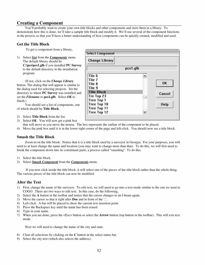
52
Creating a Component You’ll probably want to create your own title blocks and other components and store them in a library. To
demonstrate how this is done, we’ll take a sample title block and modify it. We’ll use several of the component functions
in the process so that you’ll have a better understanding of how components can be quickly created, modified and used.
Get the Title Block
To get a component from a library,
1) Select Get from the Components menu.
The default library should be
C:\pcs\pcs1.glb if you installed PC Survey
to the default directory in the installation
program.
(If not, click on the Change Library
button. The dialog that will appear is similar to
the dialog used for selecting projects. Set the
directory to where PC Survey was installed and
set the Filename to pcs1.glb. Select OK to
finish.)
You should see a list of components, one
of which should be Title Block.
2) Select Title Block from the list.
3) Select OK. You will now get a pink box
that will move as you move the mouse. The box represents the outline of the component to be placed.
4) Move the pink box until it is in the lower right corner of the page and left-click. You should now see a title block.
Smash the Title Block
Zoom in on the title block. Notice that it is a title block used by a surveyor in Georgia. For your purposes, you will
need to at least change the name and location (you may want to change more than that). To do this, we will first need to
break the component down into its constituent parts, a process called “smashing”. To do this,
1) Select the title block.
2) Select Smash Component from the Components menu.
If you now click inside the title block, it will select one of the pieces of the title block rather than the whole thing.
The various pieces of the title block can now be modified.
Alter the Text
1) First, change the name of the surveyor. To edit text, we will need to go into a text mode similar to the one we used in
COGO. There are two ways to edit text. In this case, do the following,
2) Select the A button in the toolbar and notice that the cursor changes to an I-beam again.
3) Move the cursor so that it right after Doe and in front of the ‘,’.
4) Left-click. A bar will be placed to show the current text insertion point.
5) Press the Backspace key until the name has been erased
6) Type in your name.
7) When you are done, press the <Esc> button or select the Arrow button (top button in the toolbar). This will exit text
mode.
Next we will need to change the name of the city and state.
8) Clear all selections by clicking on the C button in the select status bar.
9) Select the city text (which also selects the address).

53
10) Select Edit Text from the Edit menu. This time it will pop up a dialog box showing the text. This box works like
other edit boxes.
11) Delete any text you want to get rid of and add any new text.
12) Select OK when you are done.
Using these methods, change the text to be anything that you want.
Creating a new component
Once a desired component has been drawn, the component can be created in the following manner:
1) Draw a selection box around all of the pieces that need to be in the title block. Make sure that everything is selected
that you want in the title block and nothing is selected that will not be a part of it.
2) Select Create from the Components menu.
3) Provide a name for the component (Title, for example).
4) Select OK.
At this point, the component exists in the project. But it has
not yet been put into a library where it can recalled for later use.
The program will now ask if you would like to place your
component in a library with the dialog shown to the right.
5) Select yes. You will now be prompted for the
library in which to put the new component.
The default library will be displayed
(C:\PCS\GLIB\PCS1.GLB). You can change
this if you want with the Change Library
button, but let’s leave it as it is.
6) Select OK. The new component will now be
inserted in the library.
Add a Certification
Next, let’s add a certification to this
plat and use the text already stored in a file
on the computer.
1) Select Block Text in the Draw menu.
2) Press the File button. Make sure that
the directory is c:\pcs or wherever the
job was put. There should be a file
named exempt.txt.
3) Select exempt.txt from the list and then
click on Open. When we get back to
the Edit Text dialog box, the text from
the file is now in the edit box as shown
in the picture to the right.
4) Select OK. The dialog will close and
there will be a box cursor on the screen.
5) Put the cursor at the upper left of where
you would like to place the text and
left-click. The text will appear within a bounding box that can be stretched and moved when the text is selected.
Adding graphic primitives
The certification would look a lot better with a box around it.

54
1) Select the box icon from the tool buttons or select Box from the Draw menu. The cursor will change to a cross-hairs
cursor to remind you that you are in a drawing mode.
2) Move the cursor to one of the corners for the new box.
3) Click the left button and move the mouse to the opposite corner. A pink box will show
where the box is being placed.
4) Left-click one more time - the pink box will become black to show the box that was
created. The cursor is still a cross-hairs to show that you can now create another box
if you want to.
Click on the Selection Cursor in the toolbar to return to editing/selection mode! You can also press the <Esc> key.
If you want to change the line type, select the box (left-click on it or left-click and drag across it). Select Line Style
from the Edit menu. Pick a linetype from the types displayed and select OK.
Perhaps you don’t like its placement? Use the move technique to change its placement.
Make it smaller? Make it larger? Select the box. Notice the nibs that appear at the corners and centers of the lines.
When the cursor is on top of one of the nibs, it will turn into a crosshairs cursor. Click and drag one of the nibs to alter the
box’s size.
Let’s print it out Time to print out what we have
created. Select Print from the Project
menu.
The most important thing here is to
make sure that the printer is correct. If
the printer listed at the top of this dialog
box is not the one that you want to use,
click on the down arrow button to show
all currently installed printers. If the
printer you need is in this list, click on the
printer. If the printer you need is not in
this list, it will need to be installed.
Consult the Windows reference manuals
for information on installing printer
drivers. If you do not have the printer
driver that you need, you will need to
contact the printer company to find out if
they have a Windows’ driver and get a
copy of it if they do.
When you have your printer set up,
click OK in the Print dialog and the job
will be printed out, assuming of course that the printer is turned on and is ready to print. Wow. You have just completed
your first project with PC Survey. You can go back to COGO and alter the arrangement of text at any time - the Layout
sheet will be updated automatically. You might want to try turning off the points (done quickly through the Visibility
command in the COGO View menu) and rearranging or deleting the texts to improve the appearance of your plot. You
can also play with the linetypes (make sure targeted lines are selected first) and point symbols (Edit Individually or
Modify Group in the Points menu of COGO). Experiment. Consult the reference manual for more information or call
technical support for suggestions or help.
Epilogue This tutorial has hopefully successfully introduced you to the basic elements of PC Survey. You should now have a
pretty good feel for how the system works. The next step is to read through the reference manual for more ideas on what
can be done. There are many functions that we have not discussed (Leader Lines, Tables, Auto Draw, User-defined
linestyles, etc.) in this tutorial, but they are thoroughly documented in the reference manual. We hope that this program
will enhance your productivity by reducing the amount of time necessary to generate your drawings and maintain your
project data.
Selection
Cursor