PDE Lecture Notes

Based in part on Rhonda Hughes’ Lecture NotesText: Partial Differential Equations by Walter Strauss

Paul Melvin

0 Introduction

Partial differential equations (PDEs) arise as models of physical, biological and economicphenomena (e.g. Maxwell’s equations for the electromagnetic field, Schrodinger’s equationin quantum theory, Black-Scholes equation for pricing derivatives) and are also fundamentaltools in many areas of pure and applied mathematics. The use of PDEs is a two-fold process:One must first formulate a PDE for a given problem (i.e. construct the mathematical model),and then figure out how to solve it. The former is an art; we will focus on the latter.

Some history: In the 18th century, basic problems in continuum mechanics (vibratingstrings, fluid dynamics) were formulated by Euler, Bernoulli and d’Alembert as PDEs, butit was not until Fourier’s treatise in 1807 that a systematic means of solving these problemswas proposed. Fourier’s paper, although initially rejected, was awarded a prize after itsresubmission in 1812. His definitive book on the subject was published in 1822, givinguniform solutions to many of the major PDEs of the time including the wave and heatequations, and Laplace’s equation.

These three equations (with auxiliary initial or boundary conditions) will be the focus ofthis course. Along the way, we will develop the basics of Fourier analysis, a subject whichoccupies a central role in applied mathematics as well as many areas of pure mathematics,including representation theory, number theory, geometry and topology. Fourier analysis hasalso stimulated the development of many new fields, e.g. wavelet analysis.

What is a PDE?

A PDE is an equation containing partial derivatives of an unknown multivariable func-tion (instead of single-variable function as for ODEs). It relates the independent variablest, x, y, . . . (where t always denotes time, while x, y, . . . typically denote “spatial” variables),the dependent variable u, and the partial derivatives of u † and so can be written

F (x, t, u, ux, ut) = 0 or F (x, t, ux, ut, uxx, uxt, utt) = 0 etc.

for suitable F . A solution to the PDE is a function u(x, y, . . . ) that satisfies this equation,at least in some region of the independent variable space.

†Often denote partial derivatives by subscripts: ux = ∂u∂x

, uxy = ∂2u∂y∂x

, . . . (Recall that if u is C2, i.e. twicecontinuously differentiable, then all mixed partials are equal: uxy = uyx, etc.) Also write ∂x as shorthand forthe “differential operator” ∂/∂x, etc., so for example ux = ∂xu and uxy = ∂xyu = ∂y∂xu.

1

Examples † (all with two independent variables x and t, or x and y)

1. (transport) ut + cux = 0 (where c is a constant)

2. (wave equation) utt = c2uxx

3. (diffusion/heat equation) ut = kuxx (where k > 0 is constant)

4. (Laplace’s equation) uxx + uyy = 0

5. (Poisson’s equation) uxx + uyy = f(x, y) (for any function f)

6. (Schrodinger’s equation) ut = i~uxx + f(x)u (where i =√−1)

7. (Black-Scholes equation) ut + x2uxx + xux − u = 0

8. (Klein-Gordon equation) utt − c2uxx +m2u+ gu3 = 0

9. (Korteweg-deVries equation) ut + uxxx + 6uux = 0

Terminology

Order The order of a PDE is the order of the highest partial derivative that occurs. Forexample equation 1 is first order, 2–8 are second order, and 9 is third order.

Linearity A PDE is called homogeneous linear if, when written in the form L(u) = 0(where L is a differential operator, e.g. L = ∂t − k∂xx in the heat equation), the operator Lis linear, meaning

L(u+ v) = L(u) + L(v) and L(cu) = cL(u)

for any functions u and v, and constant c. What this really means is that L(u) is a linearcombination of u and its partial derivatives with coefficients that are constants or functionsof the independent variables. A PDE of the form L(u) = f(x, t, . . . ) with L linear and fnot identically zero is called an inhomogeneous linear PDE. For example, equations 1–7 arelinear (all homogeneous except Poisson’s equation) while 8 and 9 are not (because of the lastterm in each case: (cu)3 6= cu3 and (cu)(cu)x 6= cuux).

†Equations 2–6 and 8 can be framed in higher dimensions, replacing uxx (+uyy) by the Laplacian of u

∆u := uxx + uyy + · · · (summed over all the spatial variables x, y, . . . )

and f by a (suitable) function of all the spacial variables.Recall from vector analysis that the Laplacian operator ∆ := ∂xx + ∂yy + · · · can also be written as the

“square” ∇2 = ∇ · ∇ of the familiar “del operator” ∇ = (∂x, ∂y, · · · ), and

grad(u) = ∇u div(v) = ∇ · v curl(v) = ∇× v

for any scalar field u and vector field v in R3. This notation is generally used to describe PDEs in higherdimensions, including Maxwell’s equations for the electric and magnetic fields E and B (in a vacuum):

Et = c∇×B and Bt = −c∇×E and ∇ ·E = ∇ ·B = 0

where c is the speed of light. This is a system of twelve PDEs involving six unknown functions (the componentsof E and B) of four independent variables (x, y, z and t).

2

Why is linearity important?

Principle of superposition The solutions of a homogeneous linear PDE form a vectorspace, ie. if u1, . . . , un are solutions and c1, . . . , cn are scalars, then

∑ciui is also a solution.

It will be seen in the next section that solving a first order linear PDE reduces to thesolution of some associated first order (but not necessarily linear) ODEs, and in many casesof interest this is easily accomplished.†

Our focus in this course will be on second order linear PDEs in two independent variables

Auxx + 2Buxy + Cuyy +Dux + Euy + Fu = G

where A–G are constants or functions of x and y. (The reason for the 2 will be seen later.)Such equations, which include many of the important PDEs in applications, are classifiedinto three types according to the sign of ∆ = AC −B2:

1. elliptic if ∆ > 0

2. parabolic if ∆ = 0

3. hyperbolic if ∆ < 0

The prototypes are Laplace’s equation, the heat equation, and the wave equation, resp.Indeed any second order linear PDE with constant coefficients can be transformed into oneof these by a suitable change of variables (see below). If the coefficients are functions, then ofcourse the type of the PDE may vary in different regions of the independent variable space.

The solutions for these three types of PDEs have very different characters. For example,it will be seen below that for the heat equation ut = kuxx, a local variation in the initialconditions will be felt instantly at any distance, in contrast to the wave equation utt = c2uxxin which the propagation speed for such a variation is finite (indeed equal to c).

Linear change of variables

A change of variables x, y r, s can often help solve a PDE. This change is linear ifit is of the form r = ax + by and s = cx + dy with ad − bc 6= 0 (the last condition =⇒the change is reversible). Now the chain rule gives ux = urrx + ussx = aur + bus anduy = urry + ussy = bur + dus. In other words

∂x = a∂r + c∂s and ∂y = b∂r + d∂s

Solving for ∂r, ∂s in terms of ∂x, ∂y (for example using matrices) gives ∂r = m(d∂x− c∂y) and∂s = m(−b∂x + a∂y) where m = 1/(ad− bc). This shows that (after renaming the variables)� �

� �substituting

{s = bx− ayr = anything

converts a∂x + b∂y into a multiple of ∂r (∗)

Remember this as s = inner − outer (or a multiple); we’ll call it the io (or oi) substitution.The usefulness of this substitution is illustrated in some of the examples below.†It will be assumed that the reader is familiar with a few basic kinds of ODEs, including first order separable

equations y′ = f(x)g(y) (solved by separating variables dy/g(y) = f(x)dx and then integrating; e.g. y′ = ayhas solution y = ceay) and first order linear equations y′+p(x)y = q(x) (solved by multiplying through by the“integrating factor” f(x) = exp(

Rp(x)dx), converting the equation into (f(x)y)′ = f(x)q(x), with solution

y = f(x)−1Rf(x)q(x)dx). Also the second order equation y′′+c2y = 0 (with solution y = a cos(cx)+b sin(cx)).

3

Solutions to some simple PDEs : Find all u(x, y) satisfying

i1 ux = 0. If this were an ODE, then one integration would give u = c for constant c.Since this is a PDE (depending also on y) this constant can be any function f(y) of y.So the general solution is

u(x, y) = f(y)

where f is an arbitrary function of one variable. (We implicitly assume that f isdifferentiable enough, once in this case, to be plugged into the PDE.)i2 2ux+3uy = 0. The change of variables r = 2x+3y and s = 3x−2y (the io-substitution)converts this equation into ur = 0 (since ux = 2ur + 3us and uy = 3ur − 2us by thechain rule, so 2ux + 3uy = 13ur = 0 =⇒ ur = 0). This has solution u = f(s), i.e.

u(x, y) = f(3x− 2y)

for arbitrary f (verify this).i3 uxx = 0. Integrating wrt x gives ux = f(y), and then again wrt x gives

u(x, y) = f(y)x+ g(y)

for arbitrary f and g.i4 uxx + u = 0. The corresponding ODE has solution u = a cosx+ b sinx where a and bare constants, so the general solution to the PDE is

u(x, y) = f(y) cosx+ g(y) sinx.

for arbitrary f and g.i5 uxy = 0. Integrating wrt y gives ux = h(x), and then wrt x gives f(x) + g(y) wheref ′ = h. So the general solution is

u(x, y) = f(x) + g(y)

for arbitrary f and g. As we will see in §3 below, the unbounded wave equation reducesto this equation by a simple change of variables.i6 uxx−uxy−2uyy = 0. The change of variables r = x−y and s = 2x+y (the io-substitutionapplied twice since the operator ∂xx−2∂xy−∂yy factors as (∂x+∂y)(∂x−2∂y); might aswell call it the oioi-substitution!) converts this equation into urs = 0. This has solutionu = f(r) + g(s), i.e.

u(x, y) = f(x− y) + g(2x+ y)

for arbitrary f and g. The reader should verify that this is indeed a solution.

Moral Solutions of PDEs involve arbitrary functions (instead of constants as for ODEs).

4

1 First order linear equations

We only treat the case of two independent variables

a(x, y)ux + b(x, y)uy + p(x, y)u = q(x, y)

although similar methods work in general.

First assume p = q = 0

Case 1 Constant coefficients aux + buy = 0 (with a, b 6= 0)

Two approaches:

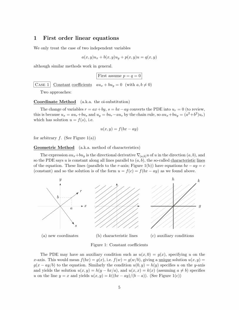
Coordinate Method (a.k.a. the oi-substitution)

The change of variables r = ax+by, s = bx−ay converts the PDE into ur = 0 (to review,this is because ux = aur+bus and uy = bur−aus by the chain rule, so aux+buy = (a2+b2)ur)which has solution u = f(s), i.e.

u(x, y) = f(bx− ay)

for arbitrary f . (See Figure 1(a))

Geometric Method (a.k.a. method of characteristics)

The expression aux+buy is the directional derivative∇(a,b)u of u in the direction (a, b), andso the PDE says u is constant along all lines parallel to (a, b), the so-called characteristic linesof the equation. These lines (parallels to the r-axis; Figure 1(b)) have equations bx− ay = c(constant) and so the solution is of the form u = f(c) = f(bx− ay) as we found above.

x

y

r

s

a

b

h

g

k

(a) new coordinates (b) characteristic lines (c) auxiliary conditions

Figure 1: Constant coefficients

The PDE may have an auxiliary condition such as u(x, 0) = g(x), specifying u on thex-axis. This would mean f(bx) = g(x), i.e. f(w) = g(w/b), giving a unique solution u(x, y) =g(x− ay/b) to the equation. Similarly the condition u(0, y) = h(y) specifies u on the y-axisand yields the solution u(x, y) = h(y − bx/a), and u(x, x) = k(x) (assuming a 6= b) specifiesu on the line y = x and yields u(x, y) = k((bx− ay)/(b− a)). (See Figure 1(c))

5

Example Find u(x, t) satisfying the initial value problem (IVP)

2ut + 3ux = 0 and u(x, 0) = sinx.

Without the initial condition we get (by either method) u(x, t) = f(2x− 3t). Thus u(x, 0) =f(2x) = sinx =⇒ f(w) = sin(w/2) =⇒ the unique solution is u(x, t) = sin(x− 3t/2).

Case 2 Variable coefficients a(x, y)ux + b(x, y)uy = 0

The coordinate method would require a nonlinear change of variables, so we use thegeometric method instead.

For example consider the equation

ux + yuy = 0 or equivalently ∇(1,y)u = 0

What curves have (1, y) as tangent vectors? Curves with slope y, i.e. curves satisfying

dy/dx = y/1

which are y = cex. These are called the characteristic curves of the PDE (Figure 2(a)).

x

yA

B

(a) characteristic curves (b) auxiliary conditions

Figure 2: Variable coefficients

Now u(x, y) is constant on each curve, since by construction its derivative in the directionof its tangents vanishes,† so is given by its value at any chosen point on the curve. For exampleif we use the point of intersection with the y-axis then

u(x, cex) = u(0, ce0) = u(0, c)

which can be an arbitrary function f(c). But the value of c corresponding to any point (x, y)is c = ye−x, so the general solution is

u(x, y) = f(ye−x).

for arbitrary f .†Can check this using the chain rule: d

dxu(x, cex) = ux + cexuy = ux + yuy = 0.

6

This method works in general, reducing the solution of a(x, y)ux + b(x, y)uy = 0 to theordinary differential equation dy/dx = a(x, y)/b(x, y). If the ODE can be solved, say in theform h(x, y) = c, then the general solution to the PDE is u(x, t) = f(h(x, y)) where f can bean arbitrary function. This is because u is constant along the solution curves h(x, y) = c ofthe ODE. These are called the characteristic curves of the PDE.

Now any auxiliary condition, which typically specifies u along some line or curve A thatintersects each characteristic at most once, will determine the solution uniquely in the regionswept out by those characteristics that do in fact intersect A (but not elsewhere). Simplyimpose the condition to determine f .

Example Solve ux + yuy = 0 (which is the PDE considered above) with each of thefollowing auxiliary conditions: (A) u(0, y) = sin y and (B) u(x, e−x) = 2x (see Figure 2(b))and discuss the uniqueness of your solution.

Solution Recall that the general solution is of the form u(x, y) = f(ye−x). Thus for (A)we have u(0, y) = f(ye0) = f(y) = sin y, and so

u(x, y) = sin(ye−x)

is the unique solution in the whole plane (since every characteristic intersects the y-axis).For (B) we have u(x, e−x) = f(e−xe−x) = f(e−2x) = 2x =⇒ f(w) = 2(−1

2 lnw) = ln(1/w),and so

u(x, y) = ln(ex/y)

is the unique solution in the upper-half plane (the union of the characteristics that intersectthe curve y = e−x). Elsewhere u can still be an arbitrary function of ye−x.

Now assume p and q are arbitrary

We will only treat the case when a and b are constant: aux + buy + p(x, y)u = q(x, y).†

Then the coordinate method (changing variables to r = ax+ by and s = bx− ay) still works,converting the equation into a linear first order ODE in the variable r (holding s constant)

(a2 + b2)ur + P (r, s)u = Q(r, s)

where P and Q are obtained from p and q by substituting x = (ar + bs)/(a2 + b2) andy = (br− as)/(a2 + b2) (these formulas come from inverting the change of variables) and theconstant of integration is replaced by a function of s as usual. The solution of this ODE willbe a function of r and s, and substituting back in terms of x and y will then solve the PDE.

Example Find the unique solution u(x, t) to the initial value problem

3ut + 4ux − 25u = 0 and u(x, 0) = sin(3x).

Solution Substitute r = 4x+3t and s = 3x−4t to get ur−u = 0, with solution u = f(s)er,so u(x, t) = f(3x − 4t)e4x+3t is the general solution of the PDE. The initial condition givesf(3x)e4x = sin(3x) =⇒ f(w) = e−4w/3 sinw and so the unique solution to the IVP is

u(x, t) = e4x+3t−4(3x−4t)/3 sin(3x− 4t) = e25t/3 sin(3x− 4t)

as is easily verified.

†If a and b are variable, then the geometric method gives the characteristic curves as solutions to the ODEdy/dx = b(x, y)/a(x, y) as before. To solve the PDE, one must parametrize each characteristic C by someparameter r, and then solve the ODE du/dr + p(r)u = q(r) along C.

7

Application: Simple transport

Consider a pollutant suspended in a fluid flowing at a constant speed c in a horizontalpipe and let u(x, t) be the concentration (mass/unit length) of the pollutant at position xand time t. Assume that the pollutant is simply carried along (transported) with the fluidas it moves, without “diffusing”. We claim that u(x, t) obeys the PDE

ut + cux = 0

To see this, note that during any time interval [t, t+ h] the fluid at position x will moveto position x+ ch, and so the corresponding concentrations will be equal

u(x+ ch, t+ h) = u(x, t).

Now differentiating with respect to h (using the chain rule on the left hand side) and puttingh = 0 gives cux + ut = 0 as claimed.

Now the solution (via the oi-substitution) is

u(x, t) = f(x− ct)

where f(x) is the initial condition u(x, 0). Geometrically this is a wave of shape u = f(x)traveling to the right at speed c, as could have been predicted without solving the PDE!

This can be illustrated by drawing a few snapshots of u(x, t) for increasing values of t, asin Figure 3

x

u

t = 0

t = 1

t = 2

Figure 3: Transport snapshots

or all in one figure:

8

2 The Wave Equation

The one-dimensional wave equation

utt = c2uxx

models the motion of vibrating strings, sound waves in a pipe, water waves in a canal, etc.Why? Here is a rough argument for the case of a string. Assume the string is flexible,

homogeneous (of constant density ρ), and stretched to a constant tension† T . Now set it inmotion, e.g. by plucking it or hitting it with a hammer. Let u(x, t) be its displacement fromequilibrium at position x and time t, so for fixed t, the graph in the xu-plane of u = u(x, t)gives the shape of the string at time t (Figure 4).

u = u(x, t)

u = u(x, t′)

h

Tux

u

x

Figure 4: Vibrating string

Assuming the vibrations are transverse (vertical motion only) the force on a small segment[x, x+ h] of the string at time t is approximately Tux(x+ h, t)− Tux(x, t) (the difference ofthe vertical components of the tensions at the ends; the horizontal components are T ). Thissegment has mass ρh and acceleration utt, and so Newton’s law F = ma becomes

T (ux(x+ h, t)− ux(x, t)) ≈ ρhutt.

Dividing by h and taking the limit as h→ 0 gives Tuxx = ρutt, i.e.

utt = c2uxx

where c =√T/ρ.

Remark This rough model ignores some forces that may affect the motion, such as

• external forces (e.g. gravity)• friction (e.g. air resistance) – proportional to velocity• restoring forces – proportional to displacement

which lead to a PDEutt = c2uxx − rut − ku+ F (x, t)

for suitable positive constants r and k, that is much harder to solve.†The tension in the string at a point is the force exerted by the part of the string to one side of the point

on the part to the other side, directed tangentially along the string because it is flexible.

9

The Infinite String (wave equation on the line R)

It is physically evident that the motion of a string with a given initial position also dependson its initial velocity. This leads to the following initial value problem for the displacementu(x, t) of the string: {

utt = c2uxx for −∞ < x <∞ and t ≥ 0u(x, 0) = φ(x), ut(x, 0) = ψ(x) for all x

The functions φ and ψ are called the initial position and initial velocity of the problem.

d’Alembert’s Formula † (1746)

Without the initial conditions, the wave equation is easily solved by changing variablessince the operator ∂tt−c2∂xx factors as (∂t−c∂x)(∂t+c∂x). In particular it reduces to urs = 0under the oioi-substitution r = x+ ct, s = x− ct and so the general solution is

u(x, t) = f(x+ ct) + g(x− ct)

where f and g are arbitrary C2 (twice continuously differentiable) functions.

Geometric Interpretation The first term f(x + ct) describes a wave of shape u = f(x)traveling to the left at speed c, while g(x − ct) is the wave u = g(x) moving to the rightat speed c. So the general solution is the superposition of two arbitrary waves moving inopposite directions, both at speed c (the speed of propagation).

gf

Figure 5: Passing waves

The lines x± ct = constant (of slopes ∓1/c) in the xt-plane are called the characteristicsof the wave equation: f(x + ct) is constant along those of negative slope while g(x − ct) isconstant along those of positive slope. These lines play an important role in the qualitativeanalysis of the wave equation (see the remarks on “causality” below).†proved independently by Euler (1748)

10

Now we impose the initial conditions u(x, 0) = φ(x) and ut(x, 0) = ψ(x) on the generalsolution u(x, t) = f(x + ct) + g(x − ct). They imply u(x, 0) = f(x) + g(x) = φ(x) andut(x, 0) = cf ′(x)− cg′(x) = ψ(x). Integrating the second equation gives cf − cg = Ψ, whereΨ is an antiderivative of ψ. This gives two equations relating the unknowns f and g:

f + g = φ and f − g = Ψ/c.

Adding these equations gives 2f = φ+ Ψ/c, and subtracting them gives 2g = φ−Ψ/2. Thusf = 1

2φ+ 12cΨ and g = 1

2φ−12cΨ, and so

u(x, t) =12

(φ(x+ ct) + φ(x− ct)) +12c

(Ψ(x+ ct)−Ψ(x− ct))

Here Ψ can be any antiderivative of ψ (they all differ by constants which cancel). This iscalled d’Alembert’s formula. It can also be written in integral form

u(x, t) =φ(x+ ct) + φ(x− ct)

2+

12c

∫ x+ct

x−ctψ(s)ds

using the fundamental theorem of calculus. This is the version given in Strauss.

Example The initial value problem utt = 4uxx, u(x, 0) = 2 sin 3x, ut(x, 0) = 6x2 hassolution u(x, t) = sin 3(x+ 2t) + sin 3(x− 2t) + 6x2t+ 8t3.

Consequences of d’Alembert’s Formula

Existence and Uniqueness of Solutions

Theorem If φ is C2 and ψ is C1, then the initial value problem for the wave equationhas a unique C2 solution given by d’Alembert’s formula.

Proof ψ is C1 =⇒ Ψ is C2 =⇒ u is C2. Thus u is a bona fide solution to the IVP.

The uniqueness of solutions has a particularly important consequence for the analysis ofwaves with boundary conditions (below):

Corollary (Parity preservation) If φ and ψ are both even or both odd,† then the solutionu(x, t) is correspondingly even or odd as a function of x (for any fixed t).

Proof If φ and ψ are even, set v(x, t) = u(−x, t). An exercise in the chain rule showsthat v satisfies the same IVP: vtt = utt(−x, t) = c2vxx, v(x, 0) = u(−x, 0) = φ(−x) = φ(x)and vt(x, 0) = ut(−x, 0) = ψ(−x) = ψ(x). By uniqueness v(x, t) = u(x, t), which says thatu(x, t) is even in x. The odd case is similar, starting with v(x, t) = −u(−x, t).

Remark This can also be proved directly from d’Alembert’s formula, noting that anyfunction that is odd or even has an antiderivative of the opposite parity.

†Recall that a function f : R→ R is even if f(−x) = f(x) for all x, and is odd if f(−x) = −f(x) for all x.

11

Causality

By d’Alembert’s formula, the value u(x, t) at any point (x, t) depends only on the valuesof φ at the two points x ± ct and the values of ψ within the interval [x − ct, x + ct] (orequivalently of Ψ at x± ct). This interval on the x-axis is called the domain of dependenceof (x, t), and is the base of a triangle, with top vertex (x, t), called the past history of (x, t)(the other two sides of this triangle are characteristics). See Figure 11(a).

domain of dependence

(x, t)

domainof

influence

pasthistory

u = 0 u = 0

support

of u

x

t

x

t

(a) past and future (b) compact supportFigure 6: Causality

Similarly the domain of influence of (x, t) is the region lying above the two characteristicsthrough (x, t). It consists of all points in the plane at which the value of u is affected in anyway by u(x, t) (Figure 11(a) again).

An important consequence of causality for waves is that

local disturbances propagate with finite speed

namely c. As an illustration, suppose that φ and ψ vanish outside a finite interval [a, b]. Thenu vanishes outside the union of the domains of influence of all the points in [a, b] (whose levelt crossection is the interval [x− ct, x+ ct]; see Figure 11(b)). (For homework you are askedwhat more can be said if ψ is zero everywhere. Hint: the domain of influence of a point onthe x-axis is then just the two upward characteristic rays emanating from the point.)

Singularities

If φ and Ψ are only piecewise C2 (meaning C2 except at a discrete set of “singular” pointswhere they need not even be continuous) then the function u given by d’Alembert’s formulawill satisfy the IVP except possibly along the characteristics through the singular points (onthe x-axis). For example consider the “triangular wave”

∧(x) :=

{1− |x| |x| < 10 |x| ≥ 1

u

x

12

which is not differentiable at ±1 and 0. Then if c = 14 , φ = ∧ (as in a “three finger pluck”)

and ψ = 0 (so we can take Ψ = 0 as well) then the snapshots of the wave (in the xu-plane )at one second intervals look like:

t = 0 t = 1 t = 2

t = 3 t = 4 t = 5

Figure 7: ∧ snapshots

Note that the snapshot at each time t is differentiable except at isolated points, namelythe points at level t in the xt-plane on the characteristics through the singularities in ∧ asshown in Figure 8.

t

x

t = 1

t = 2

Figure 8: Propagating singularities

This illustrates the principle that

singularities in the initial data are propagated along characteristics.

This can be explained in general using causality. In the homework, you are asked to makea similar analysis using a “square wave” as the initial position or initial velocity (the lattermodels a hammer striking the string, as in a piano).

13

The semi-infinite string (wave equation on the half line R+)

Suppose that one end of the string is fixed. This leads to the following “Initial BoundaryValue Problem” (IBVP) for the displacement u(x, t):

utt = c2uxx for x ≥ 0 and t ≥ 0u(x, 0) = φ(x), ut(x, 0) = ψ(x) for all xu(0, t) = 0 for all t

The restrictions in the second line are called the initial conditions (we assume that φ and ψare defined on R+ with φ(0) = ψ(0) = 0) and the last restriction is the boundary condition.

To solve this, let φodd and ψodd be the odd extensions of φ and ψ to R, i.e.

φodd(x) =

{φ(x) for x ≥ 0−ψ(−x) for x < 0

and similarly for ψodd. Let u(x, t) be the solution of the IVP on R with initial data φodd andψodd. Then by parity preservation (proved above) u(x, t) is odd in x, so u(0, t) = 0 for all t.Therefore the boundary condition is automatically satisfied, and so the restriction of u(x, t)to x ≥ 0 is the solution to the IBVP. By d’Alembert’s formula

u(x, t) = f(x+ ct) + g(x− ct)

where f = 12φodd + 1

2cΨeven and g = 12φodd− 1

2cΨeven. Here Ψeven is any antiderivative of ψodd

on R, or equivalently the even extension of any antiderivative Ψ of ψ on R+.The solution can be expressed directly in terms of φ and ψ as follows. First note that

the parity subscripts in f can be dropped since x+ ct ≥ 0. They can also be dropped for gwhen x− ct ≥ 0, but if x− ct ≤ 0 then

g(x− ct) = −12φ(ct− x)− 1

2cΨ(ct− x) = −f(ct− x).

Therefore the solution to the IBVP is

u(x, t) = f(x+ ct) +

{g(x− ct) for x ≥ ct−f(ct− x) for x ≤ ct

where f = 12φ+ 1

2cΨ and g = 12φ−

12cΨ (which are just the restrictions to R+ of the f and g

above) or in integral form

u(x, t) =

φ(x+ ct) + φ(x− ct)2

+12c

∫ x+ct

x−ctψ(s)ds for x ≥ ct

φ(ct+ x)− φ(ct− x)2

+12c

∫ ct+x

ct−xψ(s)ds for x ≤ ct

Note that these formulas agree when x = ct but that u might be singular (i.e. not differ-entiable, or even not continuous) along the characteristic x = ct. We will also call thisd’Alembert’s Formula for the half line.

14

Example The wave equation utt = 4uxx on the half line with initial conditions u(x, 0) =2 sin 3x, ut(x, 0) = 6x2 and boundary condition u(0, t) = 0 has solution

u(x, t) = sin 3(x+ 2t) + sin 3(x− 2t) +

{6x2t+ 8t3 for x ≥ 2tx3 + 12xt2 for x ≤ 2t.

Physical Interpretation: Waves reflect off the boundary

For simplicity, assume that φ and ψ vanish outside [a, b], and further that∫ ba φ(s)ds = 0,

so ψ has an antiderivative Ψ that also vanishes outside [a, b]. Then d’Alembert’s formulashows that for t < a/c, the wave is the superposition of two profiles traveling in oppositedirections at speed c.

What happens at t = a/c when the wave moving to the left reaches the boundary? Theanswer is that it temporarily changes shape (during the time interval [a/c, b/c]) and thenreturns to its original shape flipped over (i.e. rotated a half turn) and traveling back in theopposite direction. u

x

Figure 9: Wave reflection

This can be proved using d’Alembert’s Formula above or by staring at the following figureshowing the evolution of φodd: u

x

Figure 10: Why waves reflect

15

Causality (for the semi-infinite string)

D’Alembert’s integral formula for the half-line leads to the following modified pictures forthe domains of dependence and influence of a point (x, t), depending upon whether x− ct ispositive or negative. The dotted line x = ct separates the regions in which the two cases ofthe formula apply. In particular, the domain of dependence is [x− ct, x+ ct] in the first case(as with the infinite string), and [ct− x, ct+ x] in the second (due to the reflection).

domain of dependence domain of dependence

(x, t)(x, t)

domainof

influence

pasthistory

domainof

influence

pasthistory

x

t

x

t

(a) past and future (b) compact supportFigure 11: Causality on the half-line

In anticipation of the study of finite strings (where x is restricted to lie in an interval[0, `] with boundary conditions u(0, t) = u(`, t) = 0) you are encouraged to explore thecorresponding picture for causality, as suggested by the following figure.

`x

t

Figure 12: Causality in a finite interval

16

We will treat this later from a different point of view, using Fourier series, but it is instructiveand of historical interest to reconcile the two perspectives (cf. Strauss pp. 61–64).

3 The Heat Equation

The one-dimensional heat equation (a.k.a. the diffusion equation)

ut = kuxx

models the flow of heat in a rod, the diffusion of a chemical in a tube of liquid, etc.Why? The easiest situation to understand is a chemical, such as a dye, diffusing in a tube

of motionless liquid. Let u(x, t) be the concentration (mass / unit length) of dye at positionx and time t. Then the mass of dye in any given interval [a, b] at a fixed time t is

m =∫ b

au(x, t)dx

Of course m changes with time at a rate equal to net rate of flow of dye into the interval.By experimental observation, the dye flows from regions of higher to lower concentration ata rate proportional to its concentration gradient (Fick’s law of diffusion) and so the net rateof flow is dm/dt = kux(b, t) − kux(a, t) for some positive constant k.† But dm/dt can alsobe computed by differentiating the integral expression for m above (using Theorem 1 in theAppendix of Strauss to interchange the order of differentiation and integration) giving∫ b

aut(x, t)dx = k(ux(b, t)− ux(a, t)) =

∫ b

akuxx(x, t)dx

where the last equality follows from the fundamental theorem of calculus. This is true for allintervals [a, b], so the integrands must be equal, which is the diffusion equation.

Similarly heat flows from hot to cold at a speed proportional to the temperature gradient(Fourier’s law) so if u(x, t) denotes the temperature of a rod at position x and time t, thesame argument (with heat content replacing mass) leads once again to the heat equation.

Solving the unbounded heat equation

We first solve the heat equation on R (an infinite rod). Physical intuition tells us thatthere should be a unique solution once we specify an initial temperature φ(x) for all x. Thusthe temperature function u(x, t) is the solution to the initial value problem:{

ut = kuxx for −∞ < x <∞ and t > 0u(x, 0) = φ(x) for all x

For theoretical reasons, we assume φ is absolutely integrable (meaning that∫∞−∞ |φ| is finite)

although the formulas we derive hold more generally (e.g. for constant φ).

†To understand the signs, consider the possibilities. If ux(b, t) > 0 then there is more dye to the right of bthan to the left, so the dye flows into the interval. If ux(a, t) > 0 then the dye flows out of the interval.

17

This turns out to be much harder to solve than the wave equation. For fun we writedown the solution right away, and then (after a remark) explain how it is derived. Here it is:

u(x, t) =1√

4πkt

∫ ∞−∞

e−(x−y)2/4ktφ(y) dy

We shall call this Fourier’s Formula.

Remark The integral in Fourier’s formula cannot generally be evaluated in closed form,but if φ is piecewise constant then it can be expressed in terms of the error function

Erf(x) =2√π

∫ x

0e−p

2dp

from statistics.† To see this, note that the substitution p = (y − x)/√

4kt leads to analternative form of Fourier’s formula:

u(x, t) =1√π

∫ ∞−∞

e−p2φ(x+ p

√4kt) dp

Now consider the characteristic function χ(a,b)(x) of the interval (a, b), which by definitionhas value 1 for x ∈ (a, b) and zero elsewhere (any piecewise constant function is a linearcombination of such functions). If φ = χ(a,b), then the integral above reduces to

1√π

∫ (b−x)/√

4kt

(a−x)/√

4kte−p

2dp

which yields the solution

u(x, t) =12

(Erf(

x− a√4kt

)− Erf(x− b√

4kt))

(since Erf is odd)

This formula can also be applied when a or b is infinite, since Erf(±∞) = ±1.†

Our derivation of Fourier’s formula will use the notion of the Fourier transform, whicharises in connection with Fourier integrals. Fourier integrals play the same role for absolutelyintegrable functions that Fourier series play for periodic functions. Although we will studyFourier series in some detail later, we describe the basic set up here:

†The integrand e−p2

in Erf is called a Gaussian. Gaussians are exponentials of quadratic functions. Theyare ubiquitous in the theory of probability and statistics (normal distributions), physics, etc. A calculusexercise shows that Z ∞

−∞e−p

2dp =

√π

It follows that Erf(±∞) = ±1, where by definition Erf(±∞) means limx→±∞ Erf(x).

18

Fourier Series

Any continuous, piecewise smooth function f : R → C of period 2π can be representedas a Fourier series

f(x) =a0

2+∞∑k=1

(ak cos kx+ bk sin kx)

where the coefficients are computed using Euler’s formulas:

ak =1π

∫ π

−πf(x) cos kx dx and bk =

1π

∫ π

−πf(x) sin kx dx

It is convenient to write this series in complex form. Using Euler’s identity

eiθ = cos θ + i sin θ

the kth term (a.k.a. the kth-harmonic of f) ak cos kx+ bk sin kx can be rewritten as

ckeikx + c−ke

−ikx

where ck = (ak − ibk)/2 and c−k = (ak + ibk)/2. Using Euler’s formulas for ak, bk this gives

f(x) =∞∑

k=−∞cke

ikx where ck =1

2π

∫ π

−πf(x)e−ikx dx

Convergence questions will be discussed later.†

Remark If the continuity assumption on f is relaxed to piecewise continuity, and if fhas a jump discontinuity at x0, then the series converges to the average of the left and righthand limits of f(x) as x approaches x0.

Now suppose that f has period 2` instead of 2π. Then the function g(x) = f(x`/π) hasperiod 2π, and its Fourier expansion g(x) =

∑cke

ikx translates (substituting xπ/` for x inthe integral for ck) into the following Fourier expansion for f(x) = g(xπ/`)

f(x) =∞∑

k=−∞cke

ikxπ/` where ck =12`

∫ `

−`f(x)e−ikxπ/` dx

Note that if f is only defined on the interval [−`, `], then this expansion is still valid for allx in that interval (seen by considering the periodic extension of f to the whole line).

Fourier Integrals and the Fourier Transform

Any continuous, piecewise smooth function f : R→ C which is absolutely integrable (andthus nonperiodic; we shall call such a function nice) has a Fourier integral representation

f(x) =∫ ∞−∞

cωeiωx dω where cω =

12π

∫ ∞−∞

f(x)e−iωx dx

†It will be shown that the Fourier series of f converges pointwise to f(x) (i.e. substituting any numberx0 for x yields a numerical series converging to f(x0)) and that it is the only trigonometric series with thatproperty.

19

This is seen by taking the limit as ` → ∞ of the Fourier series for f on [−`, `], describedabove. Indeed, setting ωk = kπ/` and ∆ω = π/` (the difference between successive ωk’s) andthen substituting the formulas for the ck’s into the series gives

f(x) =∞∑

k=−∞

(1

2π

∫ `

−`f(y)e−iωky dy

)eiωkx∆ω

for any x ∈ [−`, `]. The right hand side looks like a Riemann sum for the Fourier integralabove, noting that ∆ω → 0 as ` → ∞. We omit the estimates required to rigorously provethat it in fact converges to that integral.

There is a beautiful symmetry inherent in the Fourier integral representation of a nicefunction, which we formulate in terms of the Fourier transform and its inverse. (In general,a transform is a linear operator that maps functions to functions.)

Definition Let f : R → C be a nice (i.e. continuous, absolutely integrable, piecewisesmooth) function. Then the functions

f(ω) =1√2π

∫ ∞−∞

f(x)e−iωx dx and f(x) =1√2π

∫ ∞−∞

f(ω)eiωx dω

are called the Fourier Transform and Inverse Fourier Transform of f , respectively. Note thatf need not be real valued, even if f is.

We also sometimes write F(f) for f , and F−1(f) for f . Fourier’s integral representationof f is simply the statement that f = F−1F(f), i.e. F and F−1 are inverse transforms.

Remark When the variable of f is spacial or temporal, written x or t, then the variableof its transform f can be interpreted as a measure of frequency, and so is written ω followingcommon physical convention.

Examples i1 The Fourier transform of f(x) = e−|x| is

f(ω) =1√2π

∫ ∞−∞

e−|x|e−iωx dx =1√2π

(∫ 0

−∞ex(1−iω) dx+

∫ ∞0

e−x(1+iω) dx

)

=1√2π

ex(1−iω)

1− iω

∣∣∣∣∣0

−∞

− e−x(1+iω)

1 + iω

∣∣∣∣∣∞

0

=1√2π

(1

1− iω− 0 + 0 +

11 + iω

)=

√2/π

1 + ω2

In this case both f and f are real valued.

i2 As will be seen below, the Fourier transform of any Gaussian is another Gaussian. Asa warm up we show (by completing the square) that e−x

2/2 is its own transform:

e−x2/2 =1√2π

∫ ∞−∞

e−x2/2e−iωx dx =

1√2π

e−ω2/2

∫ ∞−∞

e−(x+iω)2/2 dx

Substituting p = (x+ iω)/√

2 in the last integral gives√

2∫∞−∞ e

−p2 dp =√

2π. Thus

e−x2/2 = e−ω2/2

20

Properties of the Fourier Transform

1. (Linearity) F(cf + g) = cF(f) + F(g) for any nice functions f, g and any constant c.This is immediate from the linearity of the integral.

2. (Shifting) Let fc(x) = f(x− c).† Then

fc(ω) =1√2π

∫ ∞−∞

f(x− c)e−iωx dx =1√2π

∫ ∞−∞

f(u)e−iω(u+c) du = e−iωcf(ω) .

3. (Scaling) Let f c(x) = f(cx).† Then

f c(ω) =1√2π

∫ ∞−∞

f(cx)e−iωx dx =1|c|

1√2π

∫ ∞−∞

f(u)e−iωu/c du =1|c|f(ω

c)

4. (Gaussians) As an application of scaling (with f(x) = e−x2/2 as in example 2 above,

and c =√

2a) we have

F(e−ax2) =

1√2ae−ω

2/4a and F−1(e−aω2) =

1√2ae−x

2/4a

for any constant a, where the second formula follows from the first by replacing a by1/4a and applying the inverse transform. Similar formulas hold for any Gaussian.

5. (Differentiation) Suppose that f is differentiable, and that both f and f ′ are nice (inparticular absolutely integrable). Then

f ′(ω) = iωf(ω)

To see this, integrate by parts:

f ′(ω) =1√2π

∫ ∞−∞

e−iωxf ′(x) dx =1√2πe−iωxf(x)

∣∣∣∣∞−∞

+iω√2π

∫ ∞−∞

e−iωxf(x) dx.

The first term on the right is zero since |eiωx| = 1 and limx→±∞ f(x) = 0 (because f isabsolutely integrable) and the last term is iωf(ω). Thus the Fourier transform convertsdifferential equations into algebraic equations!

6. (Convolution) The convolution of two nice functions f and g is the function defined by

f ∗ g (x) :=1√2π

∫ ∞−∞

f(x− y)g(y) dy

†If c > 0 then the graph of fc is obtained by shifting the graph of f to the right by a distance c.†Then the graph of fc is obtained by horizontally scaling the graph of f by a factor of c, squeezing it in if

c > 1 and spreading it out if c < 1 (and reflecting through the vertical coordinate axis if c < 0).

21

It turns out that the Fourier transform of a product of two functions is the convolutionof their product: fg = f ∗ g . Indeed

fg(ω) =1√2π

∫ ∞−∞

f(x)g(x)e−iωx dx =1

2π

∫ ∞−∞

f(x)(∫ ∞−∞

g(σ)eiσx dσ)e−iωxdx

=1

2π

∫ ∞−∞

(∫ ∞−∞

f(x)e−i(ω−σ)x dx

)g(σ)dσ (reversing the order of integration)

=1√2π

∫ ∞−∞

f(ω − σ)g(σ)dσ = f ∗ g (ω)

Similarly f ∗ g = f g by essentially the same calculation. Thus F converts productsinto convolutions and convolutions into products, and the same is true of the F−1.

Application to filtering in image/audio processing: Multiplying the Fourier transform ofthe data function by an appropriate step function to cut off high frequencies correspondsto convolving the data function with the inverse transform of the step function.

Derivation of Fourier’s Formula (using the Fourier transform)

We seek a solution u(x, t) to the heat equation ut = kuxx with initial temperatureu(x, 0) = φ(x). Consider the function u of two variables given by

u(ω, t) =1√2π

∫ ∞−∞

u(x, t)e−iωt dx.

For any fixed t, this is just the Fourier transform of the function u(x, t), viewed as a functionof x. Observe that ut = ut (by differentiating under the integral sign) and uxx = −ω2u (bythe differentiation property 5 above). Thus ut = kuxx becomes a family of ODEs

ut = −kω2u

one for each frequency ω. Imposing the initial condition u(x, 0) = φ(x), or equivalentlyu(ω, 0) = φ(ω), these have a uniform solution

u(ω, t) = φ(ω)e−kω2t

This is the solution in the “frequency domain”. To rewrite it in the “spatial domain” we takethe inverse transform, which by Property 6 above is the convolution φ(x) with the inversetransform of e−kω

2t, denoted S(x, t). Since e−kω2t is Gaussian in ω, S(x, t) is Gaussian in x:

S(x, t) = F−1(e−kω

2t)

=1√2kt

e−x2/4kt

(computed for example using Property 4 above with a = kt) and so

u(x, t) = S(x, t) ∗ φ(x) =1√

4πkt

∫ ∞−∞

e−(x−y)2/4ktφ(y) dy

This is Fourier’s formula.

22

S

x

smallt

S

x

mediumt

S

x

larget

Figure 13: Heat Kernel

Remark The Gaussian S(x, t) is called the heat kernel, a.k.a. the source or Green’sfunction for the heat equation. Below are sketches of the graph of S(x, t) as functions of x,for various values of t.

Note that S(x, t) → 0 uniformly in x as t → ∞, and it follows that u(x, t) → 0 as well.Convolving with S(x, t) smoothes and spreads φ out more and more as time passes.

Applications of Fourier’s formula

Existence and Uniqueness of Solutions

Theorem If φ is continuous, piecewise smooth and absolutely integrable, then the heatequation ut = kuxx with initial condition u(x, 0) = φ(x) has a unique C∞ solution for t > 0,given by Fourier’s formula u(x, t) = S(x, t) ∗ φ(x) (where S(x, t) = (1/

√2kt) e−x

2/4kt).

Proof This follows from the fact that S(x, t) is C∞ (in both variables).†

As with the initial value problem for the wave equation, the uniqueness of solutions hasthe following useful consequence:

Corollary (Parity preservation) If φ is odd or even, then the solution u(x, t) is corre-spondingly odd or even as a function of x (for any fixed t).

Proof We treat odd case, leaving the even one to the reader. Set v(x, t) = −u(−x, t).An exercise in the chain rule shows that v satisfies the same IVP: vt = −ut(−x, t) = kvxxand v(x, 0) = −u(−x, 0) = −φ(−x) = φ(x). By uniqueness v(x, t) = u(x, t), which says thatu(x, t) is odd in x.

Propagation of local disturbances and singularities

There is no analogue for the heat equation of the wave causality principle. Consequentlythe principles of finite speed propagation of local disturbances and singularities for waves donot apply to heat flow. Indeed Fourier’s formula predicts very different behavior, namely

local disturbances propagate with infinite speed

†Note that the convolution of any nice function with a C∞ function is C∞. For the theoretical details, see§3.5 in Strauss.

23

i.e. they are felt immediately at all distances. Perhaps this is physically unrealistic, but it isa mathematical consequence of our simple model. Furthermore

singularities in the initial data immediately disappear

since convolving with the C∞ heat kernel smoothes out the solution.

The semi-infinite rod (heat equation on the half line R+)

Suppose that one end of a heated rod is kept at a constant temperature. This leads tothe following IBVP for the temperature u(x, t):

ut = kuxx for x ≥ 0 and t > 0u(x, 0) = φ(x) for all xu(0, t) = 0 for all t.

This is solved using the same trick as for the wave equation: Extend φ to an odd functionφodd on R. Then the restriction to x > 0 of the solution to the heat equation on the wholeline, with initial condition u(x, 0) = φodd(x), is the desired solution to the IBVP on thehalf line: it automatically satisfies the boundary condition by parity preservation. Thus byFourier’s formula the solution is

u(x, t) =1√

4πkt

∫ ∞−∞

e−(x−y)2/4ktφodd(y) dy

To write this in terms of the original function φ, split the integral into two: from −∞ to 0and from 0 to ∞. For the first we have∫ 0

−∞e−(x−y)2/4ktφodd(y) dy = −

∫ ∞0

e−(x+y)2/4ktφ(y) dy

by substituting −y for y and using the oddness of φodd, and for the second we can simplydrop the odd subscript on φ. Thus the solution to the IBVP is

u(x, t) =1√

4πkt

∫ ∞0

(e−(x−y)2/4kt − e−(x+y)2/4kt

)φ(y) dy

Remark The substitution p = (y−x)/√

4kt in the first exponential and p = (y+x)/√

4ktin the second leads to an alternative form of the formula

u(x, t) =1√π

(∫ ∞−x/√

4kte−p

2φ(p√

4kt+ x) dp−∫ ∞x/√

4kte−p

2φ(p√

4kt− x) dp

)

which is sometimes useful. For example, if φ is the characteristic function χ(a,b) then thisyields the solution

u(x, t) =12

[(Erf(

x− a√4kt

)− Erf(x− b√

4kt))

+(

Erf(x+ a√

4kt)− Erf(

x+ b√4kt

))]

.

24

(a) Erf(x) (b) Erf(x/√

4kt)

Figure 14: Constant initial temperature

In particular, if φ = 1 = χ(0,∞) then the solution is

u(x, t) = Erf(x√4kt

).

Rescaling the graph of Erf in Figure 14(a)) gives the graphs of u(x, t) for various values of t,as in Figure 14(b)).

increasingt

4 Sources

In this short section, we derive solutions to the inhomogeneous wave and heat equationson the line.† These look like the corresponding homogeneous solutions (d’Alembert’s andFourier’s formulas) but with one additional term accounting for the inhomogeneity.

Wave equation with a source

The IVP for the inhomogeneous wave equation on the line is{utt = c2uxx + f(x, t) for −∞ < x <∞, t ≥ 0u(x, 0) = φ(x) and ut(x, 0) = ψ(x) for all x

(1)

where f(x, t) should be viewed as an external force applied to the string, possibly varyingwith time. Here is the solution:

u(x, t) =12

(φ(x+ ct) + φ(x− ct)) +12c

∫ x+ct

x−ctψ +

12c

∫∫4

f

where 4 is the “past history” triangle of (x, t) in the xt-plane, with vertices v1 = (x− ct, 0),v2 = (x+ ct, 0) and v3 = (x, t).

Why is this so? Among the many approaches (see §3.4 in Strauss) perhaps the easiest issimply to appeal to Green’s Theorem, from Multivariable Calculus:†For the case of the half line with various boundary conditions, see Strauss p. 76 and pp. 67–68.

25

Green’s Theorem If P,Q : R2 → R are C1 functions and D is a region in R2 boundedby a piecewise smooth simple closed curve ∂D, then (viewing R2 as the xt-plane)∫

∂D

P dx+Qdt =∫∫D

(Qx − Pt) dx dt .

Here ∂D is by convention oriented positively (i.e. counterclockwise).

To obtain the formula for the solution u(x, t) to (3) we apply Green’s Theorem with

P (x, t) = ut(x, t) and Q(x, t) = c2ux(x, t)

and D = 4. Note that ∂4 consists of three oriented edges C1 =−→v1v2, C2 =

−→v2v3 and

C3 =−→v3v1. Also f(x, t) = utt − c2uxx = Pt −Qx and so∫∫

4

f =∫∫4

(Pt −Qx) dx dt = −∫∂4

P dx+Qdt = −(I1 + I2 + I3)

whereIk =

∫Ck

P dx+Qdt =∫Ck

ut dx+ c2ux dt.

Now along C1 we have dt = 0 and ut = φ, and so I1 =∫ x+ct

x−ctψ.

Along C2, which is part of a slope −1/c characteristic line of the differential equation,x+ct is constant and so dx+cdt = 0 =⇒ utdx+c2uxdt = −cutdt−cuxdx = −cdu. Therefore

I2 = −c∫Ck

du = −c(u(v3)− u(v2)) = c(φ(x+ ct)− u(x, t))

by the fundamental theorem of calculus, and similarly I3 = c(φ(x− ct)− u(x, t)).Putting these calculations together gives∫∫

4

f = −∫ x+ct

x−ctψ − c(φ(x+ ct) + φ(x− ct)) + 2cu(x, t)

which upon dividing by 2c and rearranging terms yields the desired formula.

Example The wave equation utt = uxx+xt with initial conditions u(x, 0) = 0 = ut(x, 0)has solution

u(x, t) =12

∫∫4

ys dy ds =12

∫ t

0

(∫ x+(t−s)

x−(t−s)y dy

)s ds

=∫ t

0x(t− s)s ds = xt3/6.

Heat equation with a source

26

The IVP for the inhomogeneous heat equation on the line is{ut = kuxx + f(x, t) for −∞ < x <∞, t > 0u(x, 0) = φ(x) for all x

(2)

where f(x, t) should be thought of as a heat source or sink. Here is the solution:

u(x, t) =1√

4πkt

∫ ∞−∞

e−(x−y)2/4ktφ(y) dy

+∫ t

0

1√4πk(t− s)

∫ ∞−∞

e−(x−y)2/4k(t−s)f(y, s) dy ds

or written in terms of convolutions (with respect to x)

u(x, t) = S(x, t) ∗ φ(x) +∫ t

0S(x, t− s) ∗ f(x, s) ds

where S(x, t) = (1/√

2kt)e−x2/4kt is the heat kernel. In physical terms this says that the

effect of the source on the temperature u(x, t) is the superposition of the impulses it providesat all the times s < t.

Now why is this the correct formula? First observe that the solution to (1) is clearly thesum of the solution u(x, t) = S(x, t) ∗ φ(x) to the associated homogeneous problem{

ut = kuxx

u(x, 0) = φ(x)

and the solution v(x, t) to the special case of (1) with φ(x) = 0:{vt = kvxx + f(x, t)v(x, 0) = 0

(3)

Thus it remains to show that v(x, t) =∫ t

0 S(x, t− s) ∗ f(x, s) ds.This is an instance of Duhamel’s Principle, which asserts in general that the solution to an

inhomogeneous PDE with homogeneous initial conditions is a superposition of solutions to theassociated homogeneous PDE with various initial conditions specified by the inhomogeneousterm in the original PDE. For the case at hand:

Claim The solution v(x, t) to (2) is a superposition of solutions vs(x, t) = S(x, t)∗f(x, s)(the convolution is with respect to x) to the family of associated homogeneous problems{

vst = kvsxxvs(x, 0) = f(x, s)

(s)

for s < t. (Note that the superscript s parametrizes the family; it is not an exponent.) Inparticular v(x, t) =

∫ t0 v

s(x, t− s) ds.

To establish the claim we verify that v(x, t) satisfies (3). Taking the partial derivativewith respect to t is tricky, however, since v(x, t) is defined by an integral in which t appears

27

both in the integration bound and in the integrand, so we appeal to the following generalresult (cf. Strauss’ Theorem 3 in Appendix A.3).

Theorem Consider the integral I(t) =∫ b(t)

a(t)g(s, t) ds where a, b : R→ R and g : R2 → R

are C1 functions. Then

I ′(t) =∫ b(t)

a(t)gt(s, t) ds+ g(b(t), t)b′(t)− g(a(t), t)a′(t)

where the gt denotes ∂g/∂t, as usual.

Proof Set J(a, b, t) =∫ ba g(s, t) ds, where a, b and t are independent variables (so I(t) =

J(a(t), b(t), t)). Then by the chain rule and the fundamental theorem of calculus, we computeI ′(t) = Jaa

′(t) +Jbb′(t) +Jt = −g(a(t), t)a′(t) + f(b(t), t)b′(t) +

∫ b(t)a(t) gt(s, t) ds, as stated.

Using this result we compute

vt(x, t) =∫ t

0vst (x, t− s) ds+ vt(x, t− t)

=∫ t

0kvsxx(x, t− s) ds+ f(x, t) = kvxx(x, t) + f(x, t)

and clearly v(x, 0) = 0. This completes the proof of the claim, and thus establishes theformula for the solution to (2).

5 Boundary Value Problems

Partial differential equations typically have many solutions. The specification of auxiliaryconditions, however, often singles one out. Up until this point we have dealt primarily withinitial conditions, although boundary conditions have arisen in our discussion of the waveand heat equations on the half line.

Boundary conditions have also arisen briefly in our discussion of the wave and heatequation on the half line, and also arise in the physically realistic situation of PDE’s on abounded domain. In particular, for functions u(x, t) of two variables (space and time) on ahalf line [a,∞) or on a finite interval [a, b], a boundary condition is a restriction on u at theendpoints a (or a and b) for all times t. The three most important types are where

• u is specified (Dirichlet boundary condition)

• ux is specified (Nemann boundary condition)

• some linear combination of u and ux is specified (Robin boundary condition)

If the condition specifies the value to be zero, then it is said to be a homogeneous condition.

Did not tex notes for the rest of this section and most of the next . . .

28

6 Fourier Series

Under construction, but here is a rough form of the last lecture in this section:

Let φ : R→ R be a 2π-periodic function.

Last time

Proved that φ is C1 =⇒ the Fourier series of φ converges pointwise to φ, i.e. for fixed x,

φ(x) =12A0 +

∞∑n=1

An cosnx+Bn sinnx (meaning RHS → φ(x)) (∗)

where (Euler’s formulas)

An =1π

∫ π

−πφ(x) cosnx dx and Bn =

1π

∫ π

−πφ(x) sinnx dx

Today: Uniform convergence Recall

1. The series∑∞

n=1 fn(x) converges uniformly to f(x) means the sequence of partial sumssN (x) =

∑Nn=1 fn(x) converges uniformly to f(x), i.e. given ε > 0, ∃M such that

N > M =⇒ |sN (x)− f(x)| < ε

for all x (stronger than pointwise convergence, where M in general depends on x).

2. The Weierstrass M -test: If ∃ constants Mn such that |fn(x)| < Mn for all x and∑Mn

converges, then∑fn(x) converges uniformly. (proof: use the Cauchy criterion)

Theorem If φ is C2, then the Fourier series of φ converges uniformly.†

Proof Integrating Euler’s formula for An twice by parts gives

An =1π

(1nφ(x) sin(nx)

∣∣∣∣π−π− 1n

∫ π

−πφ′(x) sin(nx)

)= − 1

nπ

(1nφ′(x) cos(nx)

∣∣∣∣π−π

+1n

∫ π

−πφ′′(x) cos(nx)

)= − 1

n2π

∫ π

−πφ′′(x) cos(nx)

where the first term on the right hand side in the first and second lines vanish because of the2π-periodicity of φ, φ′, sin and cos. Since φ′′ and cos are bounded, we have |An| ≤ A/n2 forsome constant A, and similarly |Bn| ≤ B/n2. Therefore

|An cosnx+Bn sinnx| ≤ A+B

n2.

†to φ, by the previous theorem

29

Since∑

1/n2 <∞, the Weierstrass M -test shows that the convergence in (∗) is uniform.

Theory application: Series solutions to PDEs

Recall (without proof) the following basic result from real analysis:

Lemma If the functions fn are differentiable on [a, b], and series∑fn and

∑f ′n both

converge uniformly (say to functions f and g respectively), then (∑fn)′ =

∑f ′n (meaning

f ′(x) = g(x)).

Using this lemma, we can finally justify the series solutions previously given for the waveand heat equations on a finite interval. For example, for the heat equation on [0, π] withNeumann boundary conditions, we have:

Theorem Let φ be a continuous function on [0, π] with Fourier cosine series coefficients

An =2π

∫ π

0φ(x) cosnx dx.

Then for each t > 0, the series

u(x, t) = 12A0 +

∑∞n=1Ane

−n2kt cosnx

converges uniformly, and satisfies the heat equation ut = kuxx with initial condition φ(x)(i.e. u(x, t) → φ(x) as t → 0) and Neumann boundary conditions ux(x, 0) = ux(x, π) = 0.Furthermore u(x, t)→ 1

2A0 as t→∞.

Proof First note that the An are uniformly bounded (independent of n) since φ is boundedon [0, π]. Now set fn(x, t) = Ane

−n2kt cosnx, the nth term in the series u(x, t), and tem-porarily fix a small s > 0.

We claim that u(x, t) =∑fn converges uniformly in x for any fixed t, and uniformly in

t > s for fixed x: Apply the Weierstrass M -test, noting that∑e−n

2ks <∞ and

|fn(x, t)| = |Ane−n2kt cosnx| ≤ Ae−n2ks

for some constant A. Similarly the series∑fn;t,

∑fn;x and

∑fn;xx

† converge uniformly,since |nfn| ≤ Bne−n

2ks and |n2fn| ≤ Cn2e−n2ks, while

∑ne−n

2ks and∑n2e−n

2ks converge.Thus, by the lemma we can differentiate term by term to obtain ut = uxx. The argument

for the limiting behavior as t→ 0 and t→∞ is left to the reader.

Similarly for the wave equation with Dirichlet boundary conditions, can prove:

Theorem Let φ be a C2 function on [0, π] with Fourier sine series coefficients

Bn =2π

∫ π

0φ(x) sinnx dx.

†where fn;t = ∂fn/∂t, etc.

30

Then the wave equation utt = c2uxx with initial position φ and initial velocity zero, andboundary conditions u(x, 0) = 0 = u(π, 0), has a unique solution given by the uniformlyconvegent series

u(x, t) =∞∑n=1

Bn cosnct sinnx =12

(φ(x+ ct) + φ(x− ct))

where φ is the odd 2π-periodic extension of φ.

Note that the last equality† relates Fourier’s approach to the heat equation to d’Alembert’sapproach. This observation was of considerable historical importance!

A remark on inhomogenous BVPs: Shifting the data

There is a useful trick to replace inhomogenous boundary conditions in a problem withhomogenous ones by subtracting a function satisfying those conditions.

For example if the problem is on the interval [0, `] with constant boundary conditionsu(0, t) = a and u(`, t) = b, then the linear function

f(x) = a+b− a`

x

clearly satisfies these conditions. Set

v(x, t) = u(x, t)− f(x).

If u satisfies a heat (or wave) equation with initial data φ (and ψ for the velocity in the wavecase) then v will satisfy the same PDE (since f is independent of t and linear in x) with“shifted” initial data φ− f (and ψ, still, in the wave case) and homogeneous boundary data.

An example of this (for the heat equation with initial temperature zero, and with a = 0and b = 10) is given in the homework. Make sure you can do this problem.

7 Laplace’s Equation

Our focus above has been on the one-dimensional wave and heat equations. In higherdimensions these equations take the form utt = c2∆u and ut = k∆u, where

∆u = uxx + uyy + · · ·

is the Laplacian of u. Here x, y, . . . are the spatial variables (so ∆u = uxx in one dimension,∆u = uxx + uyy in two, and so forth). Under suitable conditions, the solutions to theseequations approach a limit as t→∞. Such a time independent or “steady-state” solution tothe wave or heat equation therefore satisfies Laplace’s equation:

∆u = 0

Solutions to Laplace’s equation are called harmonic functions. These include all linearfunctions, and (in dimensions > 1) many others such as u(x, y) = ex sin y (check this). They†proved by plugging in the Fourier sine series expansion of φ at x±ct, and then expanding each term using

the trig identity for the sine of a sum

31

arise in many areas of mathematics and physics, including electrostatics, fluid dynamics (inthe study of an irrotational flow of an incompressible fluid), gauge theory, complex functiontheory, minimal surface theory, the study of Brownian motion, etc.

In one dimension, Laplace’s equation is simply uxx = 0 with solutions u(x) = A + Bx.There’s nothing more to it: The harmonic functions of one variable are exactly the linearfunctions. It follows that

∃ unique harmonic function on any interval with prescribed boundary values

Remarkably, this fact generalizes to higher dimensions if one substitutes for the intervalany bounded open region D in Rn with sufficiently smooth boundary ∂D:

∃ unique harmonic function on D limiting to a prescribed continuous function on ∂D

The problem of finding such a harmonic function u is called the Dirichlet problem for D,and can be quite difficult in general. The uniqueness of the resulting continuous functionu : D → R (where D = D ∪ ∂D is the closure of D) is an easy consequence of the followingbasic result:

Maximum principle Any u : D → R as above (continuous on D ⊂ Rn, harmonic on D)attains its maximum and minimum values on the boundary ∂D, i.e. there exist x0, x1 ∈ ∂Dsuch that u(x0) ≤ u(x) ≤ u(x1) for all x ∈ D.

Proof Since a minimum point for u is just a maximum point for −u (which is alsoharmonic on D) it is enough to show how to find a maximum point for u.

Let x1 be any maximum point for the restriction of u to ∂D, which exists since we areassuming D is bounded (=⇒ ∂D is compact†). We claim that x1 is the desired maximumpoint for u on all of D. In fact we will show that for every ε > 0,

u(x) < u(x1) + εs for all x ∈ D

where s is the maximum squared norm of points on ∂D, which will complete the proof byletting ε→ 0.

So given ε > 0, set v(x) = u(x) + ε ||x||2. Then

∆v = ∆u+ 2nε = 0 + 2nε > 0

(Note that ∆||x||2 = ∆(x2 + y2 + · · · ) = 2 + 2 + · · · = 2n in Rn.) Now let y be a maximumpoint for v on D, which must in fact lie in ∂D since ∆v cannot be positive at any maximumpoint of v in D (by the second derivative test in calculus). Thus for all x ∈ D we have

u(x) ≤ v(x) ≤ v(y) = u(y) + ε||y||2 ≤ u(x1) + εs

Corollary (Uniqueness of the solution to the Dirichlet problem) If u, v : D → R aresolutions to the Dirichlet problem with the same boundary condition, then u = v.

Proof The harmonic function u − v is zero on ∂D, and so zero on D by the maximumprinciple. Thus u = v on D.†From real analysis, continuous C → R with compact attains a maximum somewhere in C

32

The Dirichlet problem for the disk

Explicit solutions to Dirichlet’s problem are known for many nice regions, such as discs,annuli, wedges, squares in the plane. Here we will treat the case of discs (and their comple-ments) which leads to Poisson’s famous formula.

First observe that when one considers regions related to circles (e.g. discs, annuli andwedges) it often helps to use polar coordinates. So we begin by writing the 2-dimensionalLaplacian in polar coordinates:

∆u = urr +1rur +

1r2uθθ (∗)

If you’ve never seen this before, study pages 150–1 in Strauss where it is carefully derived.†

Now the simplest solutions to look for are the “rotationally invariant” ones u(r, θ) = u(r)(depending only on r) for which Laplace’s equation reduces to

urr +1rur = 0 or equivalently rurr + ur = (rur)r = 0

Integrating we get rur = a (a constant) =⇒ ur = a/r, and so integrating again gives

u(r, θ) = a log r + b

where a and b are constants. Of course we must have a = 0 if the region D includes theorigin (since log is undefined at 0) and so this shows in particular that the solution to theDirichlet problem on the disc with constant boundary data is constant (which we could haveguessed). If the D is an annulus (the region between two concentric circles) centered at theorigin, with u (or ur; see homework) a prescribed constant on each boundary circle, then onecan readily find a and b.

Now the general Dirichlet problem (in polar coordinates) for the disc of radius a

r2urr + rur + uθθ = 0 with u(a, θ) = h(θ)

can be solved by separating variables, and then proceeding using Fourier series, much likethe 1-dimensional heat and wave equations on an interval:

For a separated solution u(r, θ) = R(r)Θ(θ) (where Θ is 2π-periodic) the PDE becomes

r2R′′Θ +R′Θ +RΘ′′ = 0 =⇒ r2R′′/R+ rR′/R = −Θ′′/Θ

which reduces to two ODEs

Θ′′ = −λΘ and r2R′′ + rR′ − λR = 0

for some constant λ.†Similarly the 3-dimensional Laplacian is given by

∆u = uρρ +2

ρur +

1

ρ2(uφφ + cotφ uθ + csc2 φ uθθ)

as shown on page 153 of Strauss.

33

Solutions to the first equation (e.g. cos√λθ) must be 2π-periodic, which force λ = n2

for some n = 0, 1, 2, . . . . If λ = 0, then Θ′′ = 0 =⇒ Θ is linear and periodic, and thereforeconstant. For n ≥ 1 the general solution is Θ(θ) = A cosnθ+ b sinnθ, and we must also thensolve the corresponding second equation

r2R′′ + rR′ − n2R = 0

This is an example of an Euler “equidimensional” equation. Rather than discuss the generalapproach to such equations, we simply note that R = rn is a solution.† Thus for λ = n ≥ 1 wehave the solutions rn(A cosnθ+B sinnθ), which suggests the following series for the generalsolution to the PDE

u(r, θ) =12A0 +

∞∑n=1

rn(An cosnθ +Bn sinnθ)

where, by the boundary condition u(a, θ) = h(θ), the coefficients are determined by Euler’sformulas

An =1πan

∫ 2π

0h(φ) cosnφdφ and Bn =

1πan

∫ 2π

0h(φ) sinnφdφ

Example Find a harmonic function u(r, θ) on the disk of radius 3 with boundary condi-tion u(3, θ) = 2 + 5 cos θ + 7 sin 2θ. Solution: Because the boundary condition is given to usas a Fourier series, we can read off the coefficients in the formula above without integrating,namely A0 = 4, A1 = 5/3, B2 = 7/9, and the rest are zero. Thus

u(r, θ) = 2 +5r3

cos θ +7r2

9sin 2θ.

Poisson’s Formula

It is a remarkable fact that the infinite series in the formula above can be summedexplicitly. Just plug in the integral formulas for the coefficients and use the trig identity forthe cosine of a difference to get

u(r, θ) =1

2π

∫ 2π

0h(φ)Pr(θ − φ) dφ

where

Pr(θ) = 1 + 2∞∑n=1

(ra

)ncosnθ

†This is seen by direct substitution: r2n(n − 1)rn−2 + rnrn−1 − n2rn = 0. How might one arrive at thissolution? Well, it is natural to try powers rp of r, since these will at least yield terms of equal degree, and thevalues of p that work are the solutions to the algebraic equation p(p− 1) + p− n2 = p2 − n2 = 0, i.e. p = ±n.But this already gives two linearly independent solutions, rn and r−n, and so the general solution must be alinear combination of these. In our case we do not consider r−n since we want a solution on the whole disk,including its center r = 0.

34

This function Pr(θ) is called the Poisson kernel for the disk of radius a. It can expressedin closed form by substituting cosnθ = 1

2(en+ + en−) (where for convenience we set e± = e±iθ)and then summing the resulting geometric series:

Pr(θ) = 1 +∞∑n=1

(ra

)nen+ +

∞∑n=1

(ra

)nen− = 1 +

re+

a− re++

re−a− re−

=a2 − ar(e+ + e−) + r2e+e− + ar(e+ + e−)− 2r2e+e−

a2 − ar(e+ + e−) + r2e+e−

=a2 − r2

a2 − 2ar cos θ + r2

since e+e− = 1 and e+ + e− = 2 cos θ. This gives Poisson’s Formula

u(r, θ) =a2 − r2

2π

∫ 2π

0

h(φ)a2 − 2ar cos(θ − φ) + r2

dφ

for the harmonic function on the disk D of radius a, extending h(θ) on ∂D.Note the

u(0, 0) =1

2π

∫ 2π

0h(φ)dφ

This is the Mean Value Property for harmonic functions: the value at the center of any diskis the average of the boundary values.

One striking consequence is that a non-constant harmonic function cannot assume itsmaximum and minimum values in a region D except on ∂D.

35