pdf - arxiv.org e-print archive · technical report - arxiv.org january 2016 1 comparative...
TRANSCRIPT

TECHNICAL REPORT - ARXIV.ORG JANUARY 2016 1
Comparative evaluation of state-of-the-artalgorithms for SSVEP-based BCIs
Vangelis P. Oikonomou, Georgios Liaros, Kostantinos Georgiadis, Elisavet Chatzilari, Ka-terina Adam, Spiros Nikolopoulos and Ioannis Kompatsiaris
Abstract
Brain-computer interfaces (BCIs) have been gaining momentum in making human-computer interaction morenatural, especially for people with neuro-muscular disabilities. Among the existing solutions the systems relyingon electroencephalograms (EEG) occupy the most prominent place due to their non-invasiveness. However, theprocess of translating EEG signals into computer commands is far from trivial, since it requires the optimizationof many different parameters that need to be tuned jointly. In this report, we focus on the category of EEG-basedBCIs that rely on Steady-State-Visual-Evoked Potentials (SSVEPs) and perform a comparative evaluation of themost promising algorithms existing in the literature. More specifically, we define a set of algorithms for each ofthe various different parameters composing a BCI system (i.e. filtering, artifact removal, feature extraction, featureselection and classification) and study each parameter independently by keeping all other parameters fixed. Theresults obtained from this evaluation process are provided together with a dataset consisting of the 256-channel,EEG signals of 11 subjects, as well as a processing toolbox for reproducing the results and supporting furtherexperimentation. In this way, we manage to make available for the community a state-of-the-art baseline forSSVEP-based BCIs that can be used as a basis for introducing novel methods and approaches.
I. INTRODUCTION
An Electroencephalogram (EEG) can be roughly defined as the signal which corresponds to the meanelectrical activity of the brain cells in different locations of the head. It can be acquired using eitherintracranial electrodes inside the brain or scalp electrodes on the surface of the head. Some of theseelectrodes are typically used as references and are either located on the scalp or on other parts of thebody, e.g., the ear lobes. To ensure reproducibility among studies an international system for electrodeplacement, the 10-20 international system, has been defined. In this system the electrodes’ locationsare related to specific brain areas. For example, electrodes O1, O2 and Oz are above the visual cortex.Each EEG signal can therefore be correlated to an underlying brain area. Of course this is only a broadapproximation that depends on the accuracy of the electrodes’ placement.
The EEG has been found to be a valuable tool in the diagnosis of numerous brain disorders. Nowadays,the EEG recording is a routine clinical procedure and is widely regarded as the physiological “goldstandard” to monitor and quantify electric brain activity. The electric activity of the brain is usuallydivided into three categories: 1) bioelectric events produced by single neurons, 2) spontaneous activity,and 3) evoked potentials. EEG spontaneous activity is measured on the scalp or on the brain. Clinicallymeaningful frequencies lie between 0.1Hz and 100Hz. Event-related potentials (ERPs) are the changesof spontaneous EEG activity related to a specific event. ERPs triggered by specific stimuli, visual (VEP),auditory (AEP), or somatosensory (SEP), are called evoked potentials (EP). It is assumed that ERPs aregenerated by activation of specific neural populations, time-locked to the stimulus, or that they occuras the result of reorganization of ongoing EEG activity. The basic problem in analysis of ERPs is theirdetection within the larger EEG activity since ERP amplitudes are an order of magnitude smaller thanthat of the rest EEG components.
When the stimulation frequency is at low rate (<4Hz) the potentials are called transient VEPs whilestimulation on higher rate (>6Hz) produces Steady State VEPs (SSVEPs) [1]. More specifically, if aseries of identical stimuli are presented at high frequency (e.g., 8 Hz), the system will stop producingtransient responses and enter into a steady state, in which the visual system resonates at the stimulusfrequency [2]. In other words, when the human eye is excited by a visual stimulus, the brain generates
arX
iv:1
602.
0090
4v2
[cs
.HC
] 3
Feb
201
6
TECHNICAL REPORT - ARXIV.ORG JANUARY 2016 2
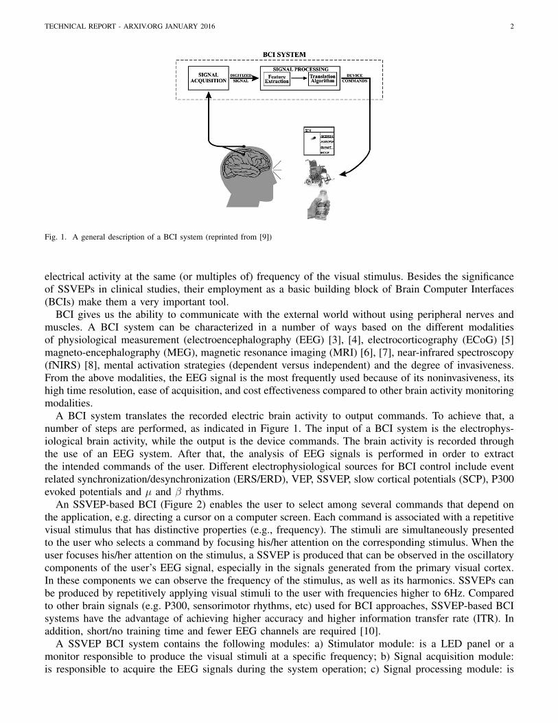
Fig. 1. A general description of a BCI system (reprinted from [9])
electrical activity at the same (or multiples of) frequency of the visual stimulus. Besides the significanceof SSVEPs in clinical studies, their employment as a basic building block of Brain Computer Interfaces(BCIs) make them a very important tool.
BCI gives us the ability to communicate with the external world without using peripheral nerves andmuscles. A BCI system can be characterized in a number of ways based on the different modalitiesof physiological measurement (electroencephalography (EEG) [3], [4], electrocorticography (ECoG) [5]magneto-encephalography (MEG), magnetic resonance imaging (MRI) [6], [7], near-infrared spectroscopy(fNIRS) [8], mental activation strategies (dependent versus independent) and the degree of invasiveness.From the above modalities, the EEG signal is the most frequently used because of its noninvasiveness, itshigh time resolution, ease of acquisition, and cost effectiveness compared to other brain activity monitoringmodalities.
A BCI system translates the recorded electric brain activity to output commands. To achieve that, anumber of steps are performed, as indicated in Figure 1. The input of a BCI system is the electrophys-iological brain activity, while the output is the device commands. The brain activity is recorded throughthe use of an EEG system. After that, the analysis of EEG signals is performed in order to extractthe intended commands of the user. Different electrophysiological sources for BCI control include eventrelated synchronization/desynchronization (ERS/ERD), VEP, SSVEP, slow cortical potentials (SCP), P300evoked potentials and µ and β rhythms.
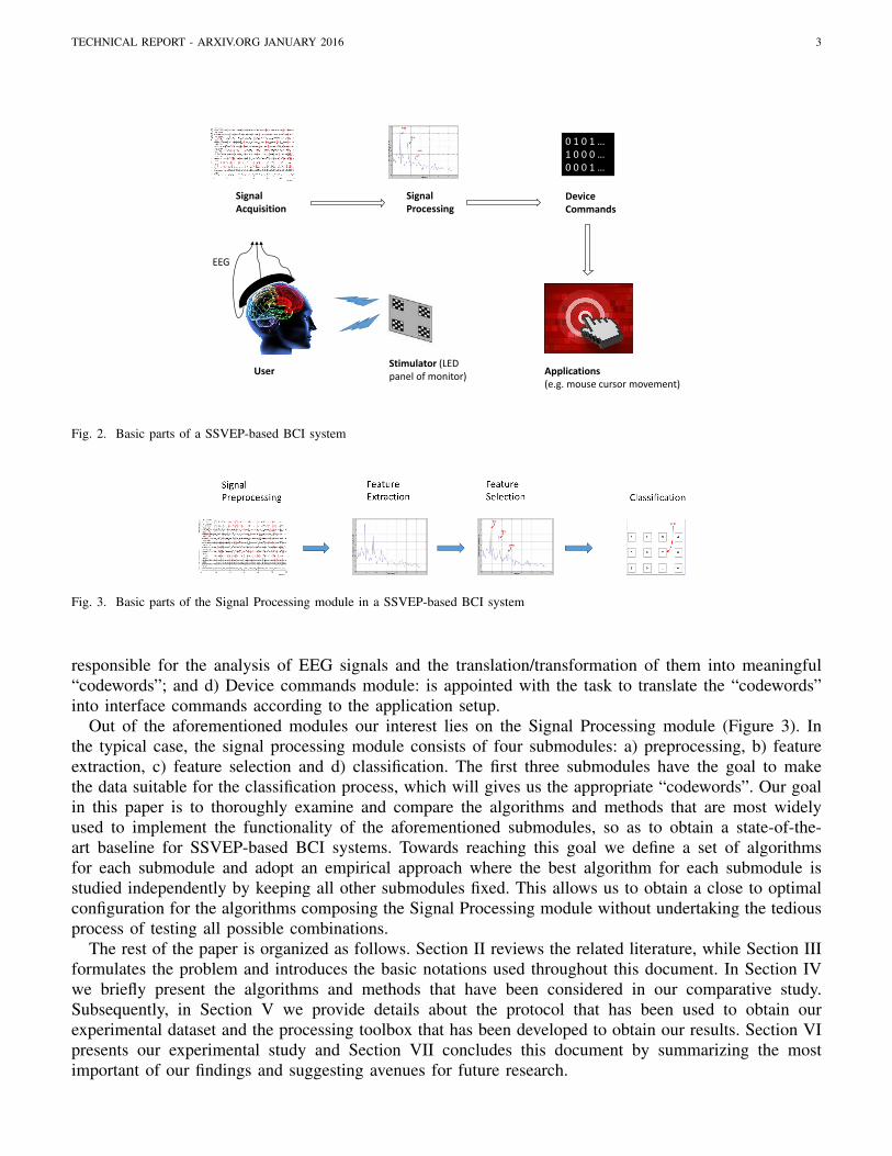
An SSVEP-based BCI (Figure 2) enables the user to select among several commands that depend onthe application, e.g. directing a cursor on a computer screen. Each command is associated with a repetitivevisual stimulus that has distinctive properties (e.g., frequency). The stimuli are simultaneously presentedto the user who selects a command by focusing his/her attention on the corresponding stimulus. When theuser focuses his/her attention on the stimulus, a SSVEP is produced that can be observed in the oscillatorycomponents of the user’s EEG signal, especially in the signals generated from the primary visual cortex.In these components we can observe the frequency of the stimulus, as well as its harmonics. SSVEPs canbe produced by repetitively applying visual stimuli to the user with frequencies higher to 6Hz. Comparedto other brain signals (e.g. P300, sensorimotor rhythms, etc) used for BCI approaches, SSVEP-based BCIsystems have the advantage of achieving higher accuracy and higher information transfer rate (ITR). Inaddition, short/no training time and fewer EEG channels are required [10].
A SSVEP BCI system contains the following modules: a) Stimulator module: is a LED panel or amonitor responsible to produce the visual stimuli at a specific frequency; b) Signal acquisition module:is responsible to acquire the EEG signals during the system operation; c) Signal processing module: is
TECHNICAL REPORT - ARXIV.ORG JANUARY 2016 3
Signal Acquisition
Signal Processing
Device Commands
Stimulator (LED panel of monitor)User
EEG
0 1 0 1 …1 0 0 0 …0 0 0 1 …
Applications (e.g. mouse cursor movement)
Fig. 2. Basic parts of a SSVEP-based BCI system
Fig. 3. Basic parts of the Signal Processing module in a SSVEP-based BCI system
responsible for the analysis of EEG signals and the translation/transformation of them into meaningful“codewords”; and d) Device commands module: is appointed with the task to translate the “codewords”into interface commands according to the application setup.
Out of the aforementioned modules our interest lies on the Signal Processing module (Figure 3). Inthe typical case, the signal processing module consists of four submodules: a) preprocessing, b) featureextraction, c) feature selection and d) classification. The first three submodules have the goal to makethe data suitable for the classification process, which will gives us the appropriate “codewords”. Our goalin this paper is to thoroughly examine and compare the algorithms and methods that are most widelyused to implement the functionality of the aforementioned submodules, so as to obtain a state-of-the-art baseline for SSVEP-based BCI systems. Towards reaching this goal we define a set of algorithmsfor each submodule and adopt an empirical approach where the best algorithm for each submodule isstudied independently by keeping all other submodules fixed. This allows us to obtain a close to optimalconfiguration for the algorithms composing the Signal Processing module without undertaking the tediousprocess of testing all possible combinations.
The rest of the paper is organized as follows. Section II reviews the related literature, while Section IIIformulates the problem and introduces the basic notations used throughout this document. In Section IVwe briefly present the algorithms and methods that have been considered in our comparative study.Subsequently, in Section V we provide details about the protocol that has been used to obtain ourexperimental dataset and the processing toolbox that has been developed to obtain our results. Section VIpresents our experimental study and Section VII concludes this document by summarizing the mostimportant of our findings and suggesting avenues for future research.

TECHNICAL REPORT - ARXIV.ORG JANUARY 2016 4
II. RELATED WORK
The study of SSVEP-based BCIs has attracted a lot of attention in what refers to the use of algorithmsand methods for maximizing the classification accuracy and improving the information transfer rate. Thenovelties that have been introduced in the literature cover the full spectrum of the Signal Processing mod-ule, ranging from signal filtering and artifact removal all the way to feature extraction and classification.In the following, we review the related literature along these lines.
Many methods have been applied in the preprocessing part of a SSVEP-BCI system. The most commonof them is the filtering, and most specifically the bandpass filtering. Various filters have been used at thispoint of analysis procedure depending of the particular needs of each SSVEP-BCI system. For examplein [11] a bandpass IIR filter from 22-48Hz is used to keep the desired parts of the EEG signal. A similarIIR filter is adopted in [12]. In another work [13] FIR filters are adopted to implement a filterbank. Inaddition, the filterbank approach is preferred to divide the EEG signal into bands [14], [15] for furtherprocessing and analysis of EEG data. Besides classical time domain filtering approaches spatial filtersare also used. More specifically, the Common Averaging Re-referencing (CAR) spatial filtering methodis used in [12] to spatially filter the multichannel EEG signals and remove unwanted components such aseye blinks. Furthermore, the Minimum Energy algorithm is used in [16] to reduce the signal - to - noiseratio between specific EEG channels. In the same spirit the method of Common Spatial Pattern (CSP)is adopted in [17], [18]. Finally, the AMUSE method in [15] and the Independent Component Analysis(ICA) in [19] are used in order to remove the noise from multichannel EEG signals.
The notion of frequency plays a central role in SSVEP BCI systems. It is typically used to generatecharacteristic features in schemes that rely on classification. Thus, we must deal with this issue with greatcaution since it affects (and it is affected by) various factors such as the experimental stimulus presentationsetup, the method that we use to estimate the resulting features (spectral analysis) and the classifier thatit is used to assign a frequency into a class. Spectral analysis methods are used to estimate/extract thefrequency of SSVEP EEG signals. More specifically, the periodogram approach is used to estimate thespectral characteristics of EEG signal in [19]–[22]. Also, a more advanced method, the Welch algorithm,is used in [12]. In addition features from time - frequency domain, using the spectrogram, are studied in[12]. Another characteristic related to the frequency, and depending of the stimulus design, is the phase.This characteristic is exploited in [23]. Finally, time domain features, such as weighted combinations ofEEG samples, are used in [15], [24]. Moreover, after extracting the features, a feature processing stepcan be introduced to further enhance the discriminative abilities of features. In this step, a selection orcombination of features is adopted. More specifically, in [19], [21], [25] spectral features are combinedempirically before feeding them into the classifier. A more advanced approach of selecting features isproposed in [12], where an incremental wrapper is used at this stage of processing.
Finally, the decision step in SSVEP BCI system is performed by applying a classification procedure.More specifically, in [12] classifiers such as the Support Vector Machine (SVM), the Linear DiscriminantAnalysis (LDA) and Extreme Learning Machines (ELM) are used. SVM and LDA are the most popularclassifiers among SSVEP community and have been used in numerous works [12], [24]–[26]. Furthermore,the adaptive network based fuzzy inference system classifier is used in [15]. Also, neural networks (NN)have been used in [26]. In [16] a statistic test is utilized in order to perform the decision, while in [21] aset of rules is applied on spectral features. In addition at this stage of procedure the Canocical CorrelationAnalysis is used. More specifically, in [11] correlation indexes using the Canonical Correlation Analysis(CCA) have been produced in order to perform the decision. Furthermore, in [14], [27] more advancedusage of CCA is adopted in order to produce similar indexes. Finally, a similar approach is proposedin [28] where a sparse regression model was fitted to the EEG data and the regression coefficients areutilized for the decision.
The existence of various options for the implementation of each submodule has motivated a non-trivial number of comparative studies for BCI systems that have been reported in the literature. In [26]a comparison study was presented with respect to the classification technique. However, the comparison

TECHNICAL REPORT - ARXIV.ORG JANUARY 2016 5
was limited between SVM and NN. Furthermore, in the feature extraction stage only features produced byFFT are used. In [12] a more exhaustive comparative study has been presented. More specifically, in thefeature extraction stage three different data sets have been produced based on spectral analysis, filterbanktheory and time - frequency domain. In addition in the feature selection stage, three feature selectionapproaches are used, two filters, the Pearson’s filter and the Davies Bouldin (DB) index, and one wrapperalgorithm. A more thorough comparative study is presented in [29] with respect to BCI systems. In thiswork the study was concentrated around numerous classification algorithms and the application of themin various BCI systems.
Motivated by the same objective, in this work we perform a systematic comparison of the algorithmsand methods that have been reported in the literature for SSVEP-based BCIs. Our contribution, comparedto existing studies, can be summarized in the following: a) our emphasis in evaluating a system that doesn’tforesee any subject-specific training prior to operation, which resulted in the adoption of the leave-one-subject-out evaluation protocol described in Section VI-B; b) the employment of an empirical approachfor multiple parameter selection that allowed us to obtain a close to optimal configuration without havingto exhaustively evaluate all possible algorithmic combinations; c) the availability of 256 channels forthe EEG signals (40 for the occipital area) that allowed us to make some very interesting remarks onthe effectiveness of different electrodes, which would have been difficult to derive with fewer channels.Finally, it is important to note that this report comes along with a dataset and a processing toolbox thathave been made public for reproducing the reported results and supporting further experimentation.
III. PROBLEM FORMULATION
Let’s assume that a SSVEP experiment is run with Ns subjects, each of whom is presented with Nt
visual stimuli (a colored light flickering at different frequencies F freq = freq1, freq2, ..., freqNfreq,
where Nfreq is the number of flickering frequencies) for a fixed duration. Each presentation of a visualstimulus corresponding to a frequency freqj is called a trial ti, i = 1, ..., Nt. During each trial ti wecapture the EEG signal eeg(ti, sk) of the subject sk. Note that in the case of SSVEPs freqj are the labelswhich we want to predict (i.e. correspond to the “codewords” mentioned above).
After the collection of the signals, we proceed with the signal processing steps shown in Figure 3.First, during the preprocessing step, we apply filtering and artifact removal to the EEG signal and weget the filtered eegf (ti, sk) and the artifact-free eega(ti, sk) signals, respectively. Afterwards, each signalis typically transformed into the frequency domain that results in a set of features eegw(ti, sk), Then,optionally, feature selection or dimensionality reduction can be applied to the features with the aim toincrease the discrimination capacity of the resulting feature space eegd(ti, sk). In the end, if we decide toemploy all aforementioned processing steps each EEG signal is represented by eegf,a,w,d(ti, sk).
After completing the aforementioned processing steps, we have a labeled dataset consisting of pairseegf,a,w,d(ti, sk), freqj, for each subject sk and trial ti, and its label freqj . This set of labeled pairsis split into train and test set, so as to facilitate the learning and testing of a classification model. Morespecifically, we employ a leave-one-subject-out cross validation scheme (see also Section VI-B) wherethe labeled pairs of all subjects except sm constitute the training set and the objective is to predict theflickering frequencies of all trials undertaken by subject sm (i.e. testing set). For simplifying the notation,let us denote by L = xi, yi (with i = 1, . . . , NL and yi ∈ F freq) the feature vectors and associatedlabels that correspond to all trials expect the ones generated from subject sm, and by U = xi, yi (withi = 1, . . . , NU and yi ∈ F freq) the feature vectors and associated labels for the trials generated fromsubject sm. This means that for the training set the index of x runs through the trials of all subjects exceptsm, i.e. NL = (Ns− 1) ·Nt, while for the test set the index of x runs through the trials generated by sm,i.e. NU = Nt. Thus, given the labeled training set L, the objective is to learn a model that will be ableto estimate a score indicating whether the stimulus flickering at freqj is the source of the EEG signalrepresented by x ∈ U (i.e. P (freqj|x)). Eventually, the EEG signal is classified to the frequency ˆfreqwhich maximizes this score:

TECHNICAL REPORT - ARXIV.ORG JANUARY 2016 6
ˆfreq = arg maxjP (freqj|x) (1)
The notations used throughout this paper can be seen in Table I.
TABLE INOTATION TABLE
Notation Meaningsi, i = 1, ..., Ns The set of Ns subjectsti, i = 1, ..., Nt The set of Nt trials for each subjectF freq =freq1, freq2, ..., freqNfreq
The set of Nfreq frequencies of the visual stimuli
eeg(ti, sk) The EEG signal of subject sk for the trial tieegf (ti, sk) The filtered EEG signal of subject sk for the trial tieega(ti, sk) The artifact-free EEG signal of subject sk for the trial ti (after
artifact removal)eegw(ti, sk) The transformation of the EEG signal into the frequency
domaineegd(ti, sk) The feature representation of the EEG signal after feature
selection or dimensionality reductionNL = ‖L‖ = (Ns − 1) ·Nt The total number of instances (trials) of all subjects except smL = X, Y = xi, yi, i =1, . . . , NL and yi ∈ F freq
The train set consisting of the final feature representations ofthe EEG signals for all subjects except sm
NU = ‖U‖ = Nt The total number of instances (trials) of the subject smU = X, Y = xi, yi, i =1, . . . , NU and yi ∈ F freq
The test set consisting of the final feature representations ofthe EEG signals for subject sm
IV. ALGORITHMS AND METHODS
In our effort to achieve a state-of-the-art baseline for SSVEP-based BCIs, we have examined a numberof algorithms and methods that are most widely used in the respective area. In this section we specifywith more detail the different algorithms and methods that have been used to implement the differentsubmodules of the signal processing module (see Figure 3).
A. Signal pre-processingInside the signal preprocessing step the data are processed in order to remove the unwanted components
of the signal. More specifically, the EEG signals are likely to carry noise and artifacts. For instance,electrocardiograms (ECGs), electrooculograms (EOG), or eye blinks affect the EEG signals. In order toremove this noise and artifacts, we can rely on the fact that EEG signals contain neuronal informationbelow 100 Hz (in many applications the information lies below 30 Hz), so any frequency component abovethese frequencies can be simply removed by using lowpass filters. Similarly a notch filter can be appliedto cancel out the 50Hz line frequency. However, when the components generated by noise and artifactslie at the effective range of EEG signals more sophisticated methods of pre-processing are necessary.
1) Signal Filtering: Between filters and spectral analysis a strong relation exists, since the goal offiltering is to reshape the spectrum of a signal in our advantage. The way that we achieve this reshapingdefines a particular filter. There is two general groups of filters, Finite Impulse Response (FIR) filters andInfinite Impulse Response (IIR) filters that are characterized by their impulse response. FIR filters referto filters that have an impulse response of finite duration, while (IIR) filters have an impulse response ofinfinite duration. Any linear system, describing the relation between the input signal eeg and the output(i.e. filtered) signal eegf , is given by:
eegf [n] =K∑k=1
a[k]eegf [n− k] +M∑m=0
b[m]eeg[n−m] (2)

TECHNICAL REPORT - ARXIV.ORG JANUARY 2016 7
where eegc[n] is the output and eeg[n] the input signal to the system at the n-th time point and a[k], k =1, · · · , K, b[m],m = 1, · · · ,M are the coefficients of the linear system. Any IIR filter is described by Eq.(2), while any FIR filter can be described by Eq. (2) when we set the a[k] coefficients to zero.
Both filter types can achieve similar results with respect to the filtering process. However differencesbetween them exists. The FIR filters are always stable and present the characteristic of linear phase [30]–[32]. In contradiction, IIR filters are not always stable and present nonlinear phase characteristics [30],[31]. However, IIR filters require fewer coefficients than FIR filters, which make them suitable for caseswhere the memory constraints are critical and some phase distortion is tolerable [30], [31]. An extensivecomparison between the two types is outside the scope of this work. The interested reader is referred to[30]–[32] for a more thorough discussion on this subject.
The most typical approach to remove noise from the EEG signal is to use band-pass filters, provided thatthe frequencies of the noise components do not overlap with the frequencies that convey the phenomenaof interest. Band pass filters work by attenuating the frequencies of specific ranges while amplifyingothers. In our case, we mainly focus on the range of 5-48Hz, which is the range defined by the stimulifrequencies (see Section V) and their harmonics (up to the 4th order). This means that we can remove alarge portion of noise related with EMG (high frequency noise), EOG (low frequency noise) and electricalcurrent (in our case 50Hz).
2) Artifact removal: Despite the filtering of the signal some noise may still persist, such as the EOGartifacts that may be present in the 0-10Hz frequency range, such as the artifacts generated from eyeblinks. For this purpose we need to follow an additional pre-processing step that is generally addressed asartifact removal. In the following, we provide details for two of most widely used approaches for artifactremoval, namely AMUSE and Independent Component Analysis.
a) AMUSE: Some of the existing techniques for artifact removal rely on blind source separation(BSS), with AMUSE [33] being one of the most typical representatives. The AMUSE algorithm havebeen used previously for artifact removal in SSVEP analysis by [15] and belongs to the second-orderstatistics spatio-temporal decorrelation algorithms [33]. AMUSE consists of two steps and each step isbased on principal component analysis (PCA). In the first step PCA is applied for whitening the data,while in the second step the singular value decomposition (SVD) is used on a time delayed covariancematrix of the pre-whitened data.
For this section let us denote the signal that is captured from all channels of the EEG sensor duringa trial as r = [r(1), . . . , r(Nchannels)], a matrix that contains the observations from all channels overtime, with r(n) being the vector that contains the observations from all channels in time n. Let us alsoassume that Rr is the covariance matrix, Rr = Er(n)rT (n). The goal of AMUSE is to decomposethe observations into uncorrelated sources, z(n) = Wr(n); or to make sure that the observations areproduced by linearly mixing uncorrelated sources, r(n) = Az(n). The first step of AMUSE aims to finda linear transformation for whitening the data, z(n) = Qr(n). The matrix Q that satisfies the whiteningproperty is Q = R
− 12
r . Next, the SVD is applied on a time delayed covariance matrix of the whitened dataz(n), Rz(n)z(n−1) = UΛV, where Λ is the diagonal matrix with decreasing singular values and U, V arethe orthogonal matrices of singular vectors. In the case of AMUSE the unmixing matrix is estimated asW = UTQ, so the estimated components are given by:
Z = Wr (3)
where r is the matrix that contains the observations from all channels over time. A useful characteristicof AMUSE is that it provides us with a ranking of components, due to the application of SVD, and thisranking is used to remove the unwanted components from the EEG signals. Based on the results reportedin the literature [15], eye blinks and other kinds of noise are typically considered to lie in the few first andlast components generated by AMUSE. Subsequently, the remaining components can be projected backto the original space using the pseudo - inverse of the unmixing matrix, aiming to yield and artifact-freeversion of the data:

TECHNICAL REPORT - ARXIV.ORG JANUARY 2016 8
r = W+Z (4)
Finally, the artifact free signal eega is the row of the matrix r corresponding to the channel we want touse.
b) Independent Component Analysis:: Another category of methods for artifact removal relies onthe use of Independent Component Analysis (ICA). Consider the matrix r of observations denoted in theprevious section. In ICA we assume that each vector r(n) is a linear mixture of K unknown sourcesz(n) = z1(n), . . . , zK(n):
r(n) = Az(n)
where the matrix of mixing coefficients A is unknown. The goal in ICA is to find the sources zi(n), orto find the inverse of the matrix A. The sources are independently distributed with marginal distributionsp(zn) = pi(z(n)(i)). The algorithm to find the independent components has three steps: a) Calculate anestimation sources through the mapping: a = Wr; b) Calculate a nonlinear mappping of the estimatedsources bi = φ(ai). A popular choice is to use the tanh function for the function φ; c) adjust the matrixW through ∆W ∝ [W−1]T + brT . The above exposition of the ICA is based on the ML principle,however similar algorithms for ICA can be obtained by adopting other criteria for the independence. Auseful introduction in ICA is presented [34], where a fast algorithm to perform ICA is also given.
From the perspective of biomedical signal processing ICA has found many applications, with the studyof brain dynamics through EEG signals being among them [35], [36]. The general application of ICAin EEG data analysis is performed in three steps. First, the EEG data are decomposed in independentcomponents, then by visual inspection some of these components are removed since they are consideredto contain artifacts (for example eyes blink), and finally the artifact-free EEG signals are obtained bymixing and projecting back onto the original channels the selected non-artifactual ICA components.
Both ICA and AMUSE are used for blind source separation. However, differences between the twoapproaches exist [33]. For example, ICA is based on high order statistics while AMUSE belongs to methodsthat use second order statistics. Also, AMUSE provides us automatically an ordering of components dueto the application of SVD (singular value decomposition). This ordering of components can be particularlyuseful in devising a general rule about which components to remove, without having to inspect the EEGdata every time.
B. Feature ExtractionAfter signal pre-processing, the feature extraction step takes place. A feature is an alternative repre-
sentation of a signal, and in most cases of lower dimensionality. Feature extraction is very importantin any pattern recognition system, since this step determines various descriptors of the signal. Also,the choice of features has an important influence on the accuracy and the computational cost of theclassification process. There are two well-known categories for extracting features: a) Nontransformedfeatures (moments, power, amplitude information, energy, etc.) and b) Transformed features (frequency andamplitude spectra, subspace transformation methods, etc.). Transformed features form the most importantcategory for biomedical signal processing and feature extraction. The basic idea employed in transformedfeatures is to find such a transformation (e.g. Fourier Transform) of the original data that best representthe relevant information for the subsequent pattern recognition task. Feature extraction is highly domain-specific and whenever a pattern recognition task is applied to a relatively new area, a key element is thedevelopment of new features and feature extraction methods.
A number of approaches can be applied in order to extract useful features for the subsequent analysisof the data. As reported in previous sections, a useful characteristic of SSVEP-based signals is thesynchronization of the brain to the frequency of the stimulus. To exploit this characteristic the frequenciescontents of EEG signals must be analyzed. The study of frequencies of a signal falls into the conceptof spectral analysis. Spectral analysis is the process of estimating how the total power of a finite length

TECHNICAL REPORT - ARXIV.ORG JANUARY 2016 9
signal is distributed over frequency. A large number of methods for estimating the spectrum (or the PowerSpectral Density - PSD) of a signal can be found in the literature. In this report we confine our study towell-known PSD methods that have been applied widely for SSVEP analysis. The objective of this stepis, given the EEG signal eeg[n], to extract a representation for it eegw using a transformation functionP ∗(f), where ∗ takes various values depending on the type of transformation (e.g. eegw = PAR(f) is theAR spectrum).
1) Periodogram: The first and most simple method for the estimation of a PSD is the periodogram [30],[31]. The periodogram is simply the Discrete Fourier Transform (DFT) of the signal. More specifically,lets assume the discrete signal eeg[n], n = 1, , N then the periodogram of eeg[n] is defined as:
P Per(f) =1
N
∣∣∣N−1∑n=0
eeg[n]e−j2πfn∣∣∣2 =
1
N|EEG(f)|2 (5)
where EEG(f) is the discrete Fourier Transform of the sequence eeg[n]. The periodogram providessome computational advantages by using the Fast Fourier Transform (FFT) algorithm to calculate theFourier Transform of eeg[n]. However, from a statistical point of view, the periodogram is an unbiasedand inconsistent estimator. This means that the periodogram does not converge to the true spectral density.Also, this estimator presents problems, related to spectral leakage and frequency resolution, due to thefinite duration of eeg[n].
2) Welch Spectrum: To reduce the above effects various non parametric methods for the estimation ofPSD were proposed. These approaches use the periodogram as a basic component of the method and atthe end provide a modified version of it. A well-known non parametric method for PSD estimation is theWelch’s method [30], [31]. This method consists of three basic steps:
1) First, divide the original N length sequence into K segments (possibly overlapped) of equal lengthsM .
eegi[m] = eeg[m+ iD], i = 0, · · · , K − 1,m = 0, · · · ,M − 1 (6)
2) Apply a window to each data segment and then calculate the periodogram on the windowed segments(modified periodograms).
Pi(f) =1
NU
∣∣∣N−1∑n=0
w[m] · eegi[m]e−j2πfm∣∣∣2, i = 0, · · · , L− 1 (7)
where U = 1M
∑M−1m=0 w[m]2 is a normalization constant with respect to the window function.
3) Average the modified periodograms from the K segments in order to obtain an estimator of thespectral density.
PW (f) =1
K
K−1∑i=0
Pi(f) (8)
The Welch estimator is a consistent estimator, but continues to present the problems of frequency resolutionand spectral leakage, although the effects of the above problems are reduced compared to the periodogram.
3) Goertzel algorithm: The basic component of the above spectrum estimation methods is the FastFourier Transform (FFT), which is used for the estimation of Discrete Fourier Transform (DFT) co-efficients. However, in the case that we want to estimate K DFT coefficients from the total N whenK << N , an alternative approach exists. This approach is called the Goertzel algorithm [30], [31]. Thebasic idea of this algorithm is that the computation of DFT coefficients can be obtained by a linear filteringoperation. When K < log2N then this algorithm is more efficient than FFT. In our study we used theGoertzel algorithm when a subset of frequencies is needed to be calculated. In the case of Goertzelalgorithm the spectrum values are obtained by applying the squaring operation on the DFT coefficients.More specifically, let EEG[f ], f = 1, · · · , K be the DFT coefficients from Goertzel algorithm, then thespectrum values are obtained as: PG(f) = |EEG(f)|2.

TECHNICAL REPORT - ARXIV.ORG JANUARY 2016 10
4) Yule - AR Spectrum: The non-parametric methods, such as the Welch method, are simple, easy toimplemented and can be calculated very fast using the FFT algorithm. However, they require large datarecords to achieve the desired frequency resolution, and, they suffer from spectral leakage effects due tofinite duration of the data. To solve these problems parametric methods have been adopted for spectralestimation. The parametric methods avoid the leakage effect while generally provide better frequencyresolution than non-parametric methods. The general idea is to assume a model that generates the dataand then, using this model, provide an estimation of spectral density. A well known parametric methodis the Yule Walker AR (PYULEAR) method [37]. This method assumes an autoregressive (AR) modelof order p for the generation of the sequence eeg[n]. Then, using the sequence eeg[n], it estimates themodel parameters. After that, the PSD is estimated according to predetermined equations. A limitation ofthe above method is how to determine the model’s order p. The Yule-AR spectrum is given by:
PAR(f) =σ2e
|1 +∑p
k=1 a[k]e−j2πfk|2(9)
where a[k], k = 1, · · · , p are the estimated AR coefficients and σ2e is the estimated minimum prediction
error.5) Short Time Fourier Transform: All the above methods make the assumption that the data are
generated from a stationary process, i.e. the frequency content of the sequence eeg[n] does not changewith the time. However, this assumption may not be hold always and the sequence eeg[n] may presentnonstationarities. To study the nonstationarities of a sequence the notion of time varying spectrum hasbeen introduced. A first approach to obtain a time varying spectrum is the Short Time Fourier Transform(STFT) [38]. The general idea of this approach is to divide the original sequence into segments andcalculate the Fourier transform in each segment. Then we can plot the spectrum of each segment toobserve the changes of frequency over time.
The Short Time Fourier Transform is given by:
S[m, f ] =N∑n=1
eeg[n]w[n−m]e−j2πfn (10)
where m = 1, 2, · · · , N, f = 0, 1N, 2N, · · · , 1 and w[·] is a preselected specialized window function.
Finally, the spectrogram is obtained as:
P S[m, f ] = |S[m, f ]|2. (11)
6) Discrete Wavelet Transform: In all above presented methods, the Fourier Transform (FT) playsthe most critical role in the method. The basic idea of FT is to represent the sequence eeg[n] as a linearsuperposition of sinusoidal waves (sines and cosines). However, sinusoidal waves are not well localized intime and hence the FT needs many coefficients to represent localized event such as a transient phenomenon.An extension of the FT is the Wavelet Transform (WT) [38] where a sequence is represented as a linearsuperposition of wavelets. Wavelets are well localized in time and frequency while the wavelet coefficientspresent sparse nature. A wavelet basis is obtained by applying careful dilations and translations of themother function ψ(n):
ψj,k(t) =1
2j/2ψ(t− 2jk
2j
)j,k∈Z
(12)
A wavelet atom ψj,k(t) is localized around the point 2jk and its support is proportional to the scale 2j . Inthe wavelet transform, the signal is represented as a linear combination of wavelets and scaling functions:
PDWT = Wg (13)
where g is the vector of wavelet coefficients and W is a matrix containing the wavelets and scalingfunctions. In practice, the wavelet coefficients are obtained by using filter banks.

TECHNICAL REPORT - ARXIV.ORG JANUARY 2016 11
C. Feature selectionAlthough the feature extraction methods are specifically designed to bring out those aspects of the data
that are most favorable in performing the intended classification task, it is rather typical to employ anadditional step that has to do with feature selection. The goal of this step is to further increase the accuracyof the classification, either by reducing the dimensionality of the feature space, and thus alleviating thecurse of dimensionality, or by removing redundant information that is likely to confuse the classifier indistinguishing between the existing classes.
With respect to the former, common approaches for dimensionality reduction use techniques fromlinear algebra such as Principal Component Analysis (PCA), Singular Value Decomposition (SVD) andIndependent Component Analysis (ICA). With respect to the latter, the approach of Feature SubsetSelection is typically followed. The general idea behind this approach is to select a subset of the availablefeatures based on some criteria, such as the entropy, the information contained in each feature, and mutualinformation, the amount of information shared by two different features, etc. While it seems that in theprocess some information will be lost, this is not the case when redundant and irrelevant features arepresent. The list of excluded features may contain features that do not have a significant impact on theoutput, or others that have a strong impact whilst they should not. In the first case the result is a morecompact representation of the features with less redundancy, whereas in the second overfitting phenomenaare avoided.
In the following we examine two algorithmic categories for feature selection, the ones relying oninformation theory and the ones resulting from the projection of the original feature space into a set ofpre-calculated components.
1) Shannon’s Information Theory: Based on Shannons Information Theory [39] and the measuresprovided below, the goal of entropy-based feature selection methods is to produce a Scoring Criterion (orRelevance Index) J that determines whether a feature is useful or not when used in a classifier. Morespecifically, the first measure is the entropy and measures the uncertainty present in the distribution of arandom variable RX using the probability distribution p(rx) of RX . In this case, we consider the featurevectors eegw to determine the probability density function (pdf) of RX .
H(RX) = −∑
rx∈RX
p(rx) log p(rx) (14)
Furthermore, conditional entropy, the second measure, is used to reduce uncertainty for rx ∈ RX whenRY is known:
H(RX|RY ) = −∑
rx∈RX
∑ry∈RY
p(rx, ry) log p(rx|ry) (15)
Mutual information is the last measure and it quantifies the amount of information shared by RX andRY . It is defined as the difference between entropy and conditional entropy:
I(RX;RY ) = H(RX)−H(RX|RY ) (16)
Based on these measurements, the 12 different indexes available on FEAST [40] aim at reducing theredundancy and/or increasing the complementary information of the features. For this purpose featuresare sorted in a descending order based on J and a subset of them S (i.e. constituting eegd) is selected forthe next steps of analysis. Thus, for each of the RXk features in the feature set (RX), J was obtainedusing the following approaches:
Jmim(RXk) = I(RXk;RY ) (17)

TECHNICAL REPORT - ARXIV.ORG JANUARY 2016 12
Mutual Information Maximization (MIM) is the Scoring Criterion that denotes the features with thehighest mutual information to a class RY , while estimating J independently for each feature.
Jmifs(RXk) = I(RXk;RY )− β∑
RXj∈S
I(RXk;RXj) (18)
Mutual Information Feature Selection (MIFS) introduces a penalty factor to the currently selected setof features to reduce redundancy. The β is a configurable parameter and when set to zero the results willbe identical to MIM Scoring Criterion.
Jjmi(RXk) =∑
RXj∈S
I(RXkRXj;RY ) (19)
Joint Mutual Information (JMI) criterion aims to increase the complementary information by including afeature to the existing set if it is complementary, while creating the joint random variable RXkRXj .
Jcmi(RXk) = I(RXk;RY |S) (20)
Conditional Mutual Information (CMI) criterion examines the information still shared by RXk and RYafter the set of all currently selected features (S) is revealed.
Jmrmr(RXk) = I(RXk;RY )− 1
|S|∑j∈S
I(RXk;RXj) (21)
Minimum - Redundancy Maximum - Relevance (MRMR) is a criterion similar to the MIFS but theconditional redundancy is omitted.
Jcmim(RXk) = I(RXk;RY )− maxRXj∈S
[I(RXk;RXj)− I(RXk;RXj|RY )] (22)
Conditional Mutual Information Maximization (CMIM) is a criterion that evaluates the features in apairwise fashion, as opposed to the previously described criteria that evaluate each feature separately.
Jicap(RXk) = I(RXk;RY )−max [0, I(RXk;RXj)− I(RXk;RXj|RY )] (23)
Interaction Capping (ICAP) criterion uses both mutual information and conditional mutual informationfor the evaluation of each feature.
Jcife(RXk) = I(RXk;RY )−∑
RXj∈S
I(RXk;RXj) +∑
RXj∈S
I(RXk;RXj|RY ) (24)
Conditional Informax Feature Selection (CIFE) criterion, similarly to ICAP, uses both mutual informa-tion and conditional mutual information with the main difference being that both these terms are boundby S and not by RXk.
Jdisr(RXk) =∑j∈S
I(RXkRXj;RY )
H(RXkRXjRY )(25)
Double Input Symmetrical Relevance (DISR) criterion introduces a normalization term (H) to the JMIcriterion.

TECHNICAL REPORT - ARXIV.ORG JANUARY 2016 13
Jbetagamma(RXk) = I(RXk;RY ) + βI(RXj;RXk) + γI(RXk;RXj|RY ) (26)
Beta Gamma criterion assigns weights (β) and (γ) to redundant mutual and conditional mutual infor-mation respectively. Using β = 0 and γ = 0 the results are equivalent to MIM scoring criterion
Jcondred(RXk) = I(RXk;RY ) + I(RXk;RXj|RY ) (27)
Conditional Redundancy (CONDRED) criterion is a special case of Beta Gamma, where β = 0 andγ = 1 and eliminates the redundant mutual information.
2) Data projection: Another approach for feature selection is the linear dimensionality reductiontechniques like Principal Component Analysis (PCA) and Singular Value Decomposition (SVD). Bothtechniques aim at mapping the original data X to a lower dimensional space using a projection matrix.More specifically, given a data matrix PCA generates a new matrix called the principal components, witheach component being the linear transformation of the data matrix. Each principal component containsthe variance, with the components being sorted in a descending order. Finally, based on the intendeddimensionality of the resulting feature space, we retain the corresponding number of principal componentsand project the original data on these components.
In SVD, the data matrix is decomposed into 3 new matrices, U and V that are unitary transforms andS that is diagonal. U × S provide the coefficients and V provides the eigenvectors. The number of theselected eigenvectors defines the desired dimensionality. The data matrix X decomposition using SVD isdefined as follows (here X refers to the training set as defined in Table I):
X = USVT (28)
Finally, we choose to retain a number of the pre-computed data components S (i.e. eigenvectors) so asto linearly project the original feature space into a new feature space (i.e. the eegd).
X = USVT (29)
Although both PCA and SVD are mostly used for reducing the dimensionality of the original space,they often increase the discrimination capacity of the data.
D. ClassificationAt the final stage of the signal processing module we encounter the classification (or pattern recognition)
algorithm. Classification is the task of assigning the EEG signals into one of several predeterminedcategories/classes. A classifier is essentially a systematic approach for building classification models froman input data set. Examples include decision tree classifiers, rule-based classifiers, neural networks, supportvector machines, and naive Bayes classifiers. Each technique employs a learning algorithm to identify amodel that best fits the relationship between the features and class label of the input data. The modelgenerated by a learning algorithm should be able to fit the input data that has been trained from, as wellas to correctly predict the class labels of records that has never seen before. Therefore, a key objectiveof the learning algorithm is to avoid overfitting and build models with good generalization capability.
Classification can be formalized as the problem of learning a mapping function y = f(x), which mapsa feature vector x to a label y. Based on the nature of the label yi, we can distinguish between binaryclassification (yi ∈ −1, 1) and multi-class classification (yi ∈ D = d1, d2, ..., dm, where D is the labelspace and dj denotes the class). In the case of multi-class classification with m classes, there are severalalgorithms that are inherently multi-class (e.g. decision trees, random forests, Adaboost, Naive Bayes,etc), which are usually probabilistic and graph based. On the contrary, similarity based algorithms (e.g.

TECHNICAL REPORT - ARXIV.ORG JANUARY 2016 14
Support Vector Machines (SVMs), Linear Discriminant Analysis (LDA), etc) being usually binary withthe objective of separating the positive from the negative class, cannot be applied directly on multi-classclassification problems. A typical way to overcome this problem is to split the multi-class problem intoseveral binary classification problems (e.g. into m binary classification problems when using the one-vs-all(OVA) trick for the transformation).
In this work we compare several popular machine learning algorithms from both categories (multi-classand binary). In the following we give a brief explanation for each of the examined algorithms.
1) Support Vector Machines (SVMs): The most popular classification algorithm is the SVMs, whichaims to find the optimal hyper-plane that separates the positive class from the negative class by maximizingthe margin between the two classes. This hyperplane, in its basic linear form, is represented by itsnormal vector w and a bias parameter b. These two terms are the parameters that are learnt during thetraining phase. Assuming that the data is linearly separable, there exist multiple hyper-planes that solvethe classification problem. SVMs choose the one that maximizes the margin, assuming that this willgeneralize better to new unseen data. This hyper-plane is found by solving the following minimizationproblem:
minw,b12‖w‖2 + C
N∑i=1
ξi
s.t.: yi(wTx + b) ≥ 1− ξi, ξi ≥ 0, i = 1, · · · , N (30)
where ξi are slack variables relaxing the constraints of perfect separation of the two classes and C is aregularization parameter controlling the trade-off between the simplicity of the model and its ability tobetter separate the two classes.
In order to classify a new unseen test example xj ∈ U , its distance from the hyper-plane is calculatedby the following equation.
f(xj) = wTxj + b (31)
It is important to note that linear SVMs are based on the assumption that the training data is linearlyseparable (i.e. there exists a set of parameters w that separates perfectly the two classes). However, thisis rarely the case for real world data. For this reason the kernel trick was introduced, which allows forthe hyper-plane to take various forms (e.g. a hyper-sphere if the RBF kernel is selected). This wasaccomplished by projecting the input data into a higher dimensional space using a Kernel functionK(xi, xj) to measure the distance between the training instances xi and xj. In this formulation, thedot product of the linear case is replaced with nonlinear kernel functions:
wTx 7→n∑i=1
wiyiK(xi,x)) (32)
In order to transform the output of the mapping function f(xj) (i.e. the distance of xj to the hyper-plane) to a probability, Platt’s sigmoid is typically used [11], [41]. This allows for using the maximizationequation (Eq. 1) without having to normalize the scores for each concept.
2) Decision Trees: A decision tree is a decision support tool that uses a tree-like graph or model ofdecisions and their possible outcomes (e.g. If the attribute xi ≥ 0 go to the left child otherwise to theleft). A decision tree is a hierarchical structure consisting of two types of nodes; a) the internal decisionnodes and b) the prediction nodes. All nodes basically examine whether a condition is satisfied, e.g.whether the value of a given attribute is higher/lower than a certain value. However, the internal decisionnodes have other nodes as children, while prediction nodes have no children and correspond to the classlabels. The advantages of decision trees are that they are simple to understand, implement and use, canlearn complicated decision boundaries and support both real valued and categorical features (attributes).However they are prone to over-fitting.

TECHNICAL REPORT - ARXIV.ORG JANUARY 2016 15
3) Ensemble Learning: Ensemble learning, based on the assumption that multiple weak classifierscan perform better than a single but more robust classifier, trains multiple classifiers either based on thesame learning algorithm (e.g. using different subsets of the training set each time) or different learningalgorithms. However, usually, the term ensemble is reserved for methods that generate multiple classifiersusing the same base learner (e.g. decision trees). Evaluating the prediction of an ensemble typically requiresevaluating the prediction of each single weak classifier and combining them. In this way, ensembles aim tocompensate for poor learning algorithms by performing a lot of extra computation. Ensemble learning canbe used in conjunction with many types of learning algorithms to improve their performance. However,fast algorithms such as decision trees are commonly used, although slower algorithms can benefit fromensemble techniques as well. In this work, we will consider the two most popular categories of ensemblelearning, boosting and bagging and as a base learning we will consider trees and discriminant classifiers.
a) Boosting: Boosting is an iterative process during which the algorithm trains a new classifierin each iteration and adapts it to the final ensemble classifier. The typical idea behind boosting is thateach new classifier aims to emphasize the training instances that previous classifiers misclassified. Byfar, the most common implementation of Boosting is AdaBoost. AdaBoost (short for Adaptive Boosting)combines the outputs of each weak classifier into a weighted sum and provides a stronger classifier byoptimizing the weights. The final classifier is proven to converge to a strong one as long as the individualweak classifiers perform at least slightly better than a random guess.
b) Bagging: Bagging (Bootstrap Aggregating), on the other hand, combines the output of the weakclassifiers in the ensemble through voting with equal weight. In order to promote model variance, baggingtrains each classifier in the ensemble using a randomly drawn subset of the training set. In the typical case,various subsets of the training set are drawn from the entire training set uniformly and with replacement.Random forests is a special case of Bagging, which uses as a base classifier the decision trees. The mainidea of Bagging that trains multiple classifiers on subsets of training data has been also widely used totackle the class imbalance problem. This problem is common in binary classification, since it is typicalto have a large number of negative examples but far fewer positive ones.
4) LDA: Linear Discriminant Analysis (LDA) works in a similar way with SVMs, by attempting tofind the separating line between the two classes. However, LDA does consider the margin between theclasses. More specifically, based on the assumption that the covariance matrices of the two classes areequal and have full rank (Σ0 = Σ1 = Σ), the optimization problem degenerates to an analytic form forthe optimal w and b as a function of the covariance matrix (Σ) and the mean (µ0,µ1):
w = Σ−1(µ1 − µ0) (33)
b =1
2(T − µ0
TΣ0−1µ0 + µ1
TΣ1−1µ1) (34)
where T is a threshold separating the two classes.5) KNN: The most popular but also simple algorithm for performing predictions is k-nearest neighbors.
In the case of KNN, the mapping function is only approximated locally. This approximation can be asimple voting scheme (i.e. the test instance is assigned to the class most common among its k nearestneighbors) or by assigning weights to the contributions of each neighbor based on their proximity to thetest instance.
6) Naive Bayes: The naive Bayes is a simple probabilistic classifier that attempts to estimate theprobability of a class ck given the features x = x1, x2, ..., xn (e.g. p(ck|x) by applying Bayes’ theorem.This method is built on a strong (naive) independence assumption, i.e. that the features are independentwithin each class. Then the probability p(ck|x) can be calculated as:
p(ck|x) = p(ck|x1, . . . , xn) =1
Zp(ck)
n∏i=1
p(xi|ck) (35)
where Z is a constant normalization factor.

TECHNICAL REPORT - ARXIV.ORG JANUARY 2016 16
V. DATA ACQUISITION & PROCESSING
A. Demographics of subjectsEleven volunteers participated in this study. They were all present employees of Centre for Research
and Technology Hellas (CERTH). Specifically, 8 of them were male and 3 female. Their ages rangedfrom 25 to 39 years old. All of them were able-bodied subjects without any known neuro-muscular ormental disorders. Subjects can also be grouped into 3 categories based on the length and thichkness oftheir hair (i.e. short hair, regular hair and thick hair). Out of the 11 subjects, there are 3 with short hair,6 with regular hair and the remaining 4 with thick hair. Finally, information about the handedness ofeach subject was also retained. Table II summarizes the demographics information about the participatingsubjects, including all the previously discussed information.
TABLE IIGENERAL INFORMATION ABOUT THE SUBJECTS
Sub. ID Age Gender Net Size Hair Type HandednessS001 24 Male Adult Medium Regular RightS002 37 Male Adult Small Regular RightS003 39 Male Adult Medium Thick RightS004 31 Male Adult Medium Short RightS005 27 Female Adult Medium Thick LeftS006 28 Female Adult Medium Thick RightS007 26 Male Adult Medium Regular RightS008 31 Female Adult Medium Thick RightS009 29 Male Adult Medium Short RightS010 37 Male Adult Medium Regular RightS011 25 Male Adult Medium Regular Right
B. Acquisition SetupThe visual stimuli was projected on a 22” LCD monitor, with a refresh rate of 60 Hz and 1680x1080
pixel resolution. The visual stimulation of the experiment was programmed in Microsoft Visual Studio2010 and OpenGL. A graphic card (Nvidia GeForce GTX 860M), fast enough to render more framesthan the screen can display, was used. Also, the option “vertical synchronization” of the graphic card wasenabled in order to ensure that only whole frames are seen on screen.
High Dimensional-EEG data were recorded with the EGI 300 Geodesic EEG System (GES 300) [42],using a 256-channel HydroCel Geodesic Sensor Net (HCGSN) and a sampling rate of 250 Hz. The contactimpedance at each sensor was ensured to be at most 80KΩ before the initialization of every new session.The synchronization of the stimulus with the recorded EEG signal was performed with the aid of theStim Tracker model ST - 100 (developed by Cedrus [43]), and a light sensor attached to the monitor thatadded markers (denoted hereafter as Dins) to the captured EEG signal. More specifically, the light sensorwas able to detect with high precision the onset of the visual stimuli and place Dins on the EEG signalfor as long as the visual stimuli flickered, providing evidence of the lasting period and the frequency ofthe stimulation. Subsequently, in the offline data processing, these Dins were used to separate the rawsignal into the part generated during the visual stimuli and the part generated during the resting period.
The stimulus of the experiment was one violet box, presented on the center of the monitor, flickering in5 different frequencies (6.66, 7.50, 8.57, 10.00 and 12.00 Hz). The box flickering in a specific frequencywas presented for 5 seconds, denoted hereafter as trial, followed by 5 seconds without visual stimulationbefore the box appears again flickering in another frequency. The background color was black for thewhole experiment.
The experiment process undertaken by each subject was divided into 5 identical sessions. Each sessionwas initiated with 100 seconds of resting period where the participant could look at the black screen ofthe monitor without being involved in any activity, followed by a 100 seconds of adaptation period (see

TECHNICAL REPORT - ARXIV.ORG JANUARY 2016 17
0 10 20 30 40 50 60 70 800
0.1
0.2
0.3
0.4
0.5
0.6
0.7
0.8
0.9
1
Fa
Fb
Fc
Fd
Fe
Ff
Fg
Fh
Bla
ck S
cree
n
Bla
ck S
cree
n
Bla
ck S
cree
n
Bla
ck S
cree
n
Bla
ck S
cree
n
Bla
ck S
cree
n
Bla
ck S
cree
n
Bla
ck S
cree
n
sec
Fig. 4. Adaptation Experimental Setup: For a period of 80 sec the five stimuli are presented randomly to the subject. Between each stimulusa resting period of 5 sec is applied.
Fig 4). The adaptation period consisted in the presentation of the 5 selected frequencies in a random wayand was considered a crucial part of the process as the subject had the opportunity to familiarize withthe visual stimulation. The following 30 second interval was left for the subject to rest and be preparedfor the next trial, which consisted in the presentation of one frequency for 3 times before another 30-second break. Every frequency is presented sequential for 3 times and with a resting period of 30 secondsbetween each trial (see Figure 5). Each session eventually includes 23 trials, with 8 of them being partof the adaptation. The entire dataset has been made publicly available in [44].
During the experiment one member of the research stuff was present giving oral instructions to thesubjects informing them about the resting time they had at their disposal and about the time they had(5 seconds) before the resting period would end and the next stimuli would appear. In addition, in aneffort to minimize the artifacts that could arise by the subject (physiological), the subjects were instructedto limit their movements and try not to swallow or blink during the visual stimulation. Furthermore,the research stuff was responsible for ensuring the correct electrode placement, the movement limitationin the experimental environment and that all mobile phones are switched off. Finally, the participantswere cautiously observed and notes were made about unexpected behavior that could lead to existenceof artifacts in the acquired signal, in order to use this information later on during the analysis of theclassification accuracy.
C. Important notesEligible signals: The EEG signal is sensitive to external factors that have to do with the environmentor the configuration of the acquisition setup. The research stuff was responsible for the elimination oftrials that were considered faulty. As a result, the following sessions were noted and excluded fromfurther analysis: i) S003, during session 4 the stimulation program crashed, ii) S004, during session 2 thestimulation program crashed, and iii) S008, during session 4 the Stim Tracker was detuned. Furthermore,we must also note that subject S001 participated in 3 sessions and subjects S003 and S004 participated in4 sessions, compared to all other subjects that participated in 5 sessions. As a result, the utilized datasetconsists of 1104 trials of 5 seconds each.Flickering frequencies: Usually the refresh rate for an LCD Screen is 60 Hz, creating a restriction tothe number of frequencies that can be selected. Specifically, only the frequencies that when divided withthe refresh rate of the screen result in an integer quotient could be selected. As a result, the frequenciesthat could be obtained were the following: 30.00, 20.00, 15.00, 12.00, 10.00, 8.57, 7.50 and 6.66 Hz.In addition, it is also important to avoid using frequencies that are multiples of another frequency, for

TECHNICAL REPORT - ARXIV.ORG JANUARY 2016 18
0 5 10 15 20 25 300
0.1
0.2
0.3
0.4
0.5
0.6
0.7
0.8
0.9
1
Bla
ck S
cree
n
Bla
ck S
cree
n
Bla
ck S
cree
n
10 H
z
10 H
z
10 H
z
sec
Fig. 5. Experimental Setup for a particular stimulus. The stimulus is presented for 5sec followed by a resting period of 5sec. The aboveprocedure is applied 3 times.
example making the choice to use 10.00Hz prohibits the use of 20.00 and 30.00 Hz. With the previouslydescribed limitations in mind, the selected frequencies for the experiment were: 12.00, 10.00, 8.57, 7.50and 6.66 Hz.Stimuli Layout: In an effort to keep the experimental process as simple as possible, we used only oneflickering box instead of more common choices, such as 4 or 5 boxes flickering simultaneously. The factthat the subject could focus on one stimulus without having the distraction of other flickering sourcesallowed us to minimize the noise of our signals and verify the appropriateness of our acquisition setup.Nevertheless, having concluded to the optimal configuration for analyzing the EEG signals, the experimentwill be repeated with more concurrent visual stimulus.Trial duration: The duration of each trial was set to 5 seconds, as this time was considered adequateto allow the occipital part of the brain to mimic the stimulation frequency and still be small enough formaking a selection in the context of a brain-computer interface. However, the investigation of the tradeoffbetween the classification accuracy and the amount of time where the flickering frequency is detected, isincluded in our immediate plans for future work.Observed artifacts: During the stimulus presentation to subject S007 the research stuff noted that thesubject had a tendency to eye blink. As a result the interference, in matters of artifacts, on the recordedsignal is expected to be high.Informed consent: Before the experiment the participants were carefully instructed about the recordingprocedure and its requirements and were provided with a form of consent to sign after reading it thoroughly.After reading the form and listening to our oral instructions, the subjects were motivated to make anyquestions regarding the procedure in an effort to eliminate misunderstandings about the process. By signingthe provided document, the participants stated their voluntary participation in the experiment and theirconsent to make their data public for research purposes. The entire experimental process has received theapproval of the ethics committee of the Centre for Research and Technology Hellas with date 3/7/2015and for the research grant with number H2020-ICT-2014-644780.
D. Processing toolboxA Matlab toolbox titled “ssvep-eeg-processing-toolbox” has been released in GitHub [45] along with
the dataset in order to setup and perform the experiments described in this paper. It follows a modulararchitecture that allows the fast execution of experiments of different configurations with minimal adjust-ments of the code. An experiment pipeline consist of five parts each of them receiving an input from theprevious part and providing an output to the next part. The Experimenter class of the toolkit acts as a

TECHNICAL REPORT - ARXIV.ORG JANUARY 2016 19
wrapper on which the parameters of the underlying parts can be specified. The parts that are given as inputto an Experimenter object are the following; a) A Session object that is used for loading the dataset andsegmenting the signal according to the stimuli markers. It is possible to load a specific session of a subject,all sessions of a specific subject or all the available sessions from all subjects. The output of a Session isa set of trials containing the EEG signal that was recorded during the presentation of the visual stimuluson the screen, annotated with the flashing frequency of the stimulus. b) A Preprocessing object can beused to apply a digital filter on the signals or perform techniques for artifact removal such as AMUSE[33]. It is also possible to select a specific channel of the captured signal or to further segment the signalin the time domain. c) A Feature Extraction object receives the processed set of trials as an input andextracts numerical features for representing the signal. Available feature extraction methods include thePWelch power spectral density estimate, Fast Fourier Transform, Discrete Wavelet Transform, etc. d) AFeature Selection object can be also optionally set for receiving the set of feature vectors produced in thefeature extraction stage and selecting the ones that are considered the most discriminative based on theirentropy or variance. For implementing the process of feature selection, a wrapper class of the FEAST [40]library is included in the toolbox, as well as methods for Principal Component Analysis or Singular ValueDecomposition. The input of the feature selection object is the number of retained dimensions and itsoutput is a set of feature vectors with reduced dimensionality. e) A Classification object is the next step ofthe experiment and includes methods for building a model given a set of annotated feature vectors and forpredicting the annotation of unseen feature vectors. Some of the included classifiers are a LIBSVM [46]wrapper class, AdaBoost and Random Forest.
The last step before running the experiment is to configure the Evaluation object of the experiment.Currently, there are two methods offered: a) “Leave one sample out” trains a classification model withn− 1 trials and tests the model with the remaining trial. The process is repeated n times until there is anoutput for each trial; b) “Leave one subject out” trains a classification model with the trials belonging ton− 1 subjects and tests the model with the trials of the remaining subject. The entire process is executedby invoking the “run” method of the Experimenter class and when the experiment is finished the resultsare available via the “results” property of the Experimenter class.
VI. EXPERIMENTAL STUDY
As already mentioned, the goal of this paper is to generate a state-of-the-art baseline for SSVEP-basedBCIs. Towards this goal, in Section I we have identified the basic parts of the signal processing module andin Section IV we have listed some of the most prominent algorithms and methods for implementing theirfunctionality. Our goal in this section is to test their performance, so as to optimally tune and configure alldifferent parts of the signal processing module leading to a state-of-the art baseline for SSVEP-based BCIs.Two measures have been used to evaluate the performance of the proposed BCI system, the classificationaccuracy and the execution time. Finally, all the experiments have been performed in an iMac computerwith a processor at 3.4GHz (Intel Core i7), memory at 8GB and an AMD Radeon (1024MB) graphicscard.
A. Multiple Parameters SelectionAs made clear in Section IV the efficiency of a SSVEP-based BCI system depends on various different
parameters (i.e. filtering, artifact removal, feature extraction, feature selection and classification) that canbe implemented by more than one algorithms. This is essentially a multi-objective parameter selectionproblem that can be tackled with methodologies such as the one presented in [47], under the restrictionthat these parameters share some heterogeneity. However, this is not the case for a SSVEP-based BCIsystem where the regulating parameters are highly heterogeneous. Thus, in our study we have adopted amore empirical approach where each parameter is studied independently by keeping all other parametersfixed.

TECHNICAL REPORT - ARXIV.ORG JANUARY 2016 20
More specifically, in order to avoid the tedious process of testing all possible combinations our approachrelies on the existence of a default configuration where the value of each parameter has been set arbitrarily(i.e. based on intuition). The role of the default configuration is two-fold; first, to provide the fixed valuesfor all parameters except the one that is being studied and second, to serve as a comparison basis in decidingwhether a certain algorithm introduces significant improvements. For example, in deciding which of thefeature extraction algorithms presented in Section IV-B is the most efficient in the context of SSVEP-based BCIs, we keep all other parameters fixed as dictated by the default configuration and alternatethe parameter dealing with feature extraction. If the improvement introduced by the best-performingalgorithm is statistically significant with respect to the performance of the default configuration, we retainthis algorithm to be part of our state-of-the-art configuration. Although we acknowledge the fact that theadopted empirical approach may not necessarily lead to the joint optimization of all different parameters,it has been favored over a brute force approach that would make the cost of experiments prohibitive.
Finally, it is important to note that in studying a certain parameter there are two different optimizationprocess. The first concerns the selection of the best competing algorithm out of the ones presented inSection IV, while the second concerns the optimal tuning of the selected algorithm with respect to itsinternal variables. Table III presents the values that have been selected for the default configurationand unless stated otherwise, are the values that have been used to undertake all experiments describedsubsequently.
TABLE IIIDEFAULT CONFIGURATION - PARAMETER VALUES
ChannelAll experiments have been performed by using the raw EEG signal fromchannel Oz. The place of channel Oz is on the midline of occipital lobe and,since we study SSVEP responses, it is the logical first choice.DurationDuration of used EEG data: all EEG trials (5sec)FitleringThe raw EEG signal have been band - pass filtered from 5-48Hz since in thisfrequency range exists the signal of interest (i.e. the various SSVEP responses).An IIR-Chebyshev I filter is used in the default configurationArtifact removalNo artifact removal algorithm is used in the default configurationFeature extractionFor feature extraction the power spectrum of Welch’s method is used with thefrequency range applied to the entire spectrum and the number of fft set to512.Feature selectionIn the default configuration we do not apply any feature selection ap-proach/algorithm.ClassificationIn the classification step we choose an SVM classifier with a linear kernel andthe cost parameter C is set to 1. Since SVMs is essentially a binary classifierthe one-vs-all approach is adopted for making this classifier applicable in ourmulti-class classification problem.
Table IV presents the classification accuracy achieved for each subject using the default configuration,

TECHNICAL REPORT - ARXIV.ORG JANUARY 2016 21
as well as the mean accuracy for all subjects and the execution time for this configuration. It is importantto note that by execution time we refer to the processing time required by each configuration to reach adecision at the testing phase (i.e. we do not consider the time required for training). In a realistic settingthis execution time should be added to the time offered to the subject in order to reach a steady state,which in our case has been set to 5 secs (i.e. the duration of one trial).
By looking at the classification results we may categorize the subjects in three different categoriesbased on their performance: a) highly-accurate where we classify all subjects with accuracy over 90%(i.e. SOO1, S009, S010 and S011), b) mid-accurate where we classify all subject with accuracy between60%-90% (i.e. S002, S004, S006, S007), and c) poorly-accurate where we classify all subjects withaccuracy below 60% (i.e. S003, S005, S008). By considering these categories in conjunction with theinformation of Table II we may reach the following conclusions. All subjects in the highly-accurate andmid-accurate categories have either short or regular hair (with the only exception of S006 that has thickhair), while all subjects in the poorly-accurate category appears to have thick hair. This observation verifiesthe knowledge obtained from literature that thick hair constitute a series obstacle in acquiring noise-freeEEG signals. Another interesting remark concerns the mid-to-poor accuracy of subject S007 that has beenobserved to excessively blink during the execution of the experiment (see Section V-C). Finally, the lastremark concerns subject S005, which is the only left-handed subject participating in our study.
TABLE IVCLASSIFICATION ACCURACY USING THE DEFAULT CONFIGURATION.
Subject ID AccuracyS001 98.55S002 87.82S003 34.78S004 77.17S005 30.43S006 86.08S007 60.00S008 31.88S009 100.0S010 92.17S011 98.26
Mean Accuracy 72.47Time (msec) 5
B. Evaluation protocolIn order to perform the necessary comparisons across the different configurations, we need to determine
an evaluation protocol that will allow us to obtain a performance indicator for each test. This procedurefalls into the model selection problem, since we have several candidate models and we wish to choosethe best of them with respect to an optimality criterion. A popular framework to choose a model amonga set of candidate models is the Cross - Validation (CV) approach [48]. The general idea of CV is tosplit the available dataset in two parts, the training set and the testing set. Then, a learning procedure foreach candidate model is performed using the training set, in order to learn/estimate the free parameter ofthe model. After that, the performance of each candidate model is evaluated with respect to the testingset. Finally, the model with the best performance in the testing set is chosen. The different variations ofCV framework are related with the splitting procedure and the metric used to quantify the performanceof the model.
In our study, we choose to employ a CV approach where the splitting procedure is performed onthe basis of subjects [48]–[50] and the performance is calculated by the accuracy of the classifier. This

TECHNICAL REPORT - ARXIV.ORG JANUARY 2016 22
approach is called Leave-One-Subject-Out (LOSO) and has been previously used to discriminate betweensensorimotor rhythms (two-class problem) in a BCI system [51]. As the name indicates the LOSO-CVapproach suggests to leave the data from one subject out of the training phase and use them only in thetesting phase of the experiment. This splitting is very important for BCI experiments since it provides usthe ability to construct general purpose systems, free of the necessity to perform subject-specific trainingprior to operation.
The LOSO - CV approach treats the EEG data quite different than a classification scheme that relieson subject-specific classifiers and work independently. More specifically, in the case of a subject-specificclassifier where both the training and testing sets are generated from the same subject, we are unable toaccount for the between - subject variability. To avoid subject-dependency one could train/test a classifierin the EEG data from all subjects belonging to the group using for example a 10-fold CV approach. Butin this approach the data from one subject are included in both the training and testing set, which reducesthe withing subject variability of the resulting classifier. To preserve the within subject variability andat the same time to take into account the between subjects variability we use a CV approach where thesplitting procedure is performed with respect to the subjects and not to the samples, such as in the caseof LOSO-CV.
C. Signal FilteringIn this series of experiments our goal is to evaluate the two basic families of filters, FIR and IIR, with
respect to the classification accuracy, and to highlight the usefulness of filtering process. Using the defaultconfiguration of our methodology we perform a comparison between filtered and raw data, as well asbetween various filters. Five basic types of filters are used as reported in Table VI. These filters are designedusing the Matlab Signal Processing Toolbox (tool filterbuilder1). In all cases the EEG trials havebeen bandpass filtered from 5-48Hz. Also, before the filtering, the EEG trials have been normalized tozero mean. The filters specifications are described in Table V. In addition to the above specifications theorder of FIR filters have been restricted to 400, while the order of IIR filters has been defined by the toolfilterbuilder. In Table VI we depict the obtained results for this series of experiments. At first, wecan see that filtering the raw signal is absolutely necessary since we achieve a classification accuracy 30%larger than without the filtering procedure. Furthermore, between the various filters we can see that theIIR filters is slightly better (0.5%) than FIR, with the IIR-Elliptic filter achieving the best performance.This difference can be explained probably by the way that each filter treats the ripples in the passbandand stopband. With respect to the execution time we see that all configurations (i.e. different filter in thiscase) provides with similar results. Based on the obtained results the IIR-Elliptic filter has been chosenfor our state-of-the-art configuration.
TABLE VSPECIFICATIONS OF FILTERS
Frequency Specifications (Hz)Stopband Frequency 1 4 Passband Frequency 1 5Passband Frequency 2 48 Stopband Frequency 2 50
Magnitude Specifications (dB)Stopband Attenuation 1 60 Passband Ripple 1Stopband Attenuation 2 60
D. Artifact RemovalOur objective in this section is to compare the artifact removal algorithms presented in Section IV-A2, as
well as to verify the positive impact of these algorithms in the final classification result. In this direction,1http://www.mathworks.com/help/dsp/ref/filterbuilder.html

TECHNICAL REPORT - ARXIV.ORG JANUARY 2016 23
TABLE VICLASSIFICATION ACCURACY USING VARIOUS FILTERS.
Sub. ID FIR Equir-rible
FIR LeastSquares
IIR Cheby-shev I
IIR Cheby-shev II
IIR Elliptic Raw EEGtrials
S001 100.0 98.55 98.55 100.0 100.0 75.36S002 86.95 87.82 87.82 90.43 89.56 33.91S003 33.33 30.43 34.78 33.33 33.33 24.63S004 79.34 80.43 77.17 79.34 78.26 39.13S005 21.73 25.21 30.43 28.69 29.56 20.86S006 86.08 84.34 86.08 86.08 86.08 39.13S007 64.34 65.21 60.00 60.86 65.21 34.78S008 33.33 36.23 31.88 33.33 34.78 21.73S009 100.0 100.0 100.0 100.0 100.0 75.65S010 93.04 91.30 92.17 92.17 91.30 40.00S011 98.26 98.26 98.26 98.26 98.26 87.82Mean Acc. 72.40 72.52 72.47 72.95 73.30 44.82Time(msec)
6 5 5 5 5 3
we have performed experiments using AMUSE and FastICA. More specifically, both algorithms havebeen applied on a trial basis (i.e. using the 5 secs of EEG signal captured in each trial) and usingall 256 channels, so as to generate the necessary components. Subsequently, the visual inspection ofthe data resulted in the identification of the components that could potentially include artifacts. Finally,different combinations of these components were removed before reconstructing the EEG signal usingthe remaining components. The components that have been retained for the signal reconstruction and theresulting accuracy of each method can be seen in Table VII.
TABLE VIIRESULTS USING ARTIFACT REMOVAL METHODS
Sub.ID
AMUSE ICA
comp 2-256 2-255 2-252 2-247 10-256
15-256
20-256
15-255
15-252
120-256
130-256
140-256
150-256
S001 98.55 98.55 97.10 97.10 100.0 100.0 91.30 100.0 100.0 17.39 30.43 21.73 21.73S002 86.95 82.60 84.34 83.47 93.91 93.04 84.34 92.17 95.65 21.73 23.47 22.60 19.13S003 33.33 42.02 40.57 42.02 33.33 46.37 39.13 47.82 40.57 15.94 21.73 21.73 23.18S004 75.00 76.08 75.00 75.00 71.73 76.08 69.56 77.17 76.08 16.30 21.73 21.73 23.91S005 26.95 24.34 24.34 20.86 23.47 25.21 20.86 24.34 32.17 21.73 16.52 15.65 18.26S006 83.47 80.00 69.56 66.95 75.65 70.43 56.52 67.82 67.82 20.86 21.73 21.73 20.86S007 69.56 74.78 84.34 88.69 92.17 90.43 72.17 90.43 95.65 19.13 21.73 21.73 21.73S008 31.88 23.18 34.78 24.63 33.33 28.98 34.78 30.43 28.98 14.49 20.28 20.28 27.53S009 99.13 99.13 99.13 99.13 100.0 100.0 98.26 100.0 100.0 23.47 21.73 33.04 32.17S010 98.26 98.26 98.26 95.65 96.52 94.78 93.91 93.04 95.65 14.78 20.86 20.86 20.00S011 98.26 98.26 98.26 98.26 98.26 93.04 85.21 93.91 93.91 14.78 31.30 20.86 22.60MeanAcc.
72.85 72.47 73.24 71.98 74.40 74.40 67.82 74.28 75.13 18.24 22.87 22.00 22.83
Time(msec)
81 73 70 68 70 69 69 70 68 5660 5660 5660 5660
It is evident from the results of Table VII that AMUSE is a reliable artifact removal method as the mean

TECHNICAL REPORT - ARXIV.ORG JANUARY 2016 24
accuracy is improved in most of the cases. The highest accuracy is achieved (75.13%) when the last fiveand the first fifteen components produced by AMUSE are excluded, with an improvement of approximately2.5% compared to the default configuration. Furthermore, it is important to notice that the accuracy forSubject S007, a Subject that was observe to blink excessively during the recordings (see Section V-C),was improved up to 30% verifying the effectiveness of AMUSE in removing the artifacts generated fromeye-blinks. On the contrary, the use of FastICA didn’t manage to introduce any improvements comparedto the default configuration, regardless of the utilized components. Also, we can see that the executiontime of AMUSE is much smaller than that of FastICA. Nevertheless, the 68 msecs required by AMUSEto remove the artifacts from the signal is a significant increase in the total execution time, compared tothe 5 msecs of the default configuration. Based on these results, the use of AMUSE combined with theremoval of the first 15 and the last 4 components, was incorporated as part of our optimal configuration.
E. Feature ExtractionIn these series of experiments our goal is to compare the discrimination ability of the feature extraction
methods presented in Section IV-B on our dataset. For all steps of the procedure, except the FeatureExtraction step, the default configuration has been used. The tuning parameters for each of the featureextraction methods have been obtained through a set of preliminary experiments and based on trial-and-error. Table VIII depicts the classification accuracy achieved using each of the feature extraction methodsalong with its tuning parameters.
We can see the superiority of Welch method as a feature extractor with respect to SSVEP experiments.This can be attributed to the averaging effect of Welch methods that seem to favor the robustness of theclassification. Also, we can see that all Fourier based methods achieve better results than the DiscreteWavelet Transform. This does not exclude the presence of non-stationarities in the EEG signal, but it isan indication that the brains synchronization with the stimulus produces a stationary process. This canbe also justified from the fact that the duration of EEG trials was 5sec, a time window large enoughfor the brain to come into a steady state situation with respect to the visual stimulus. However, not inall cases the Welch method provides the best classification results. For example, in the case of subjectS005 the wavelet transform provides us with better classification accuracy. It is worth to notice herethat the Goertzel algorithm needs more processing time than the others approaches. Based on the resultsof Table VIII, the PWelch method qualifies as the best feature extraction method to be included in ouroptimal configuration.
As depicted in Table VIII the tuning parameters of PWelch has been set to Nfft:512 and Fr. range:0-125Hz. Given that PWelch has been selected as the best-performing candidate, the next series ofexperiments aimed at further optimizing the tuning parameters of PWelch so as to increase the classificationaccuracy. More specifically, the number of FFT points, the length of the segments and the overlap betweensegments have been checked using a grid-search approach. The frequency range has been kept fixed at0-125Hz. The overall tuning procedure is described in Algorithm 1 and the accuracy of the 10 bestconfigurations resulting from this procedure is depicted in Table IX. Also, in this table we provide theaccuracy corresponding to the default values of the above parameters that have been used in Table VIII.As we can see by further tuning the PWelch method we manage to obtain an increase in accuracy around1%. However, this increase on classification is coming at the expense of 1 additional msec in the totalexecution time. From the above results it is evident that an increase in the overlap between segmentsprovides us with better accuracy (although it requires more processing time), probably due to the fact thatthe estimated frequencies are more accurate.
F. Feature SelectionIn this section we experimentally examine the effectiveness of the feature selection methods presented
in Section IV-C to increase the discrimination capacity of the feature space and lead to better classificationresults. Aiming in the investigation of the features selection parameter, the default configuration was used
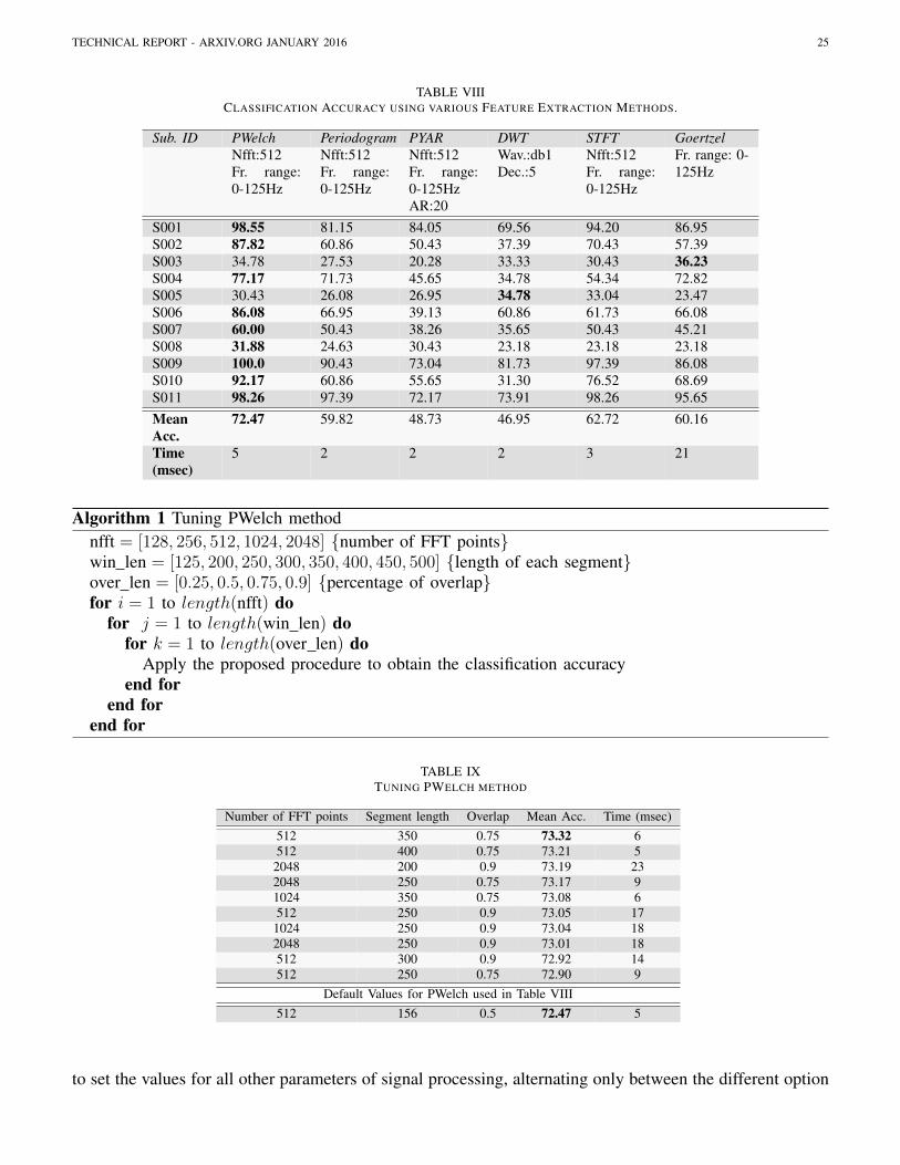
TECHNICAL REPORT - ARXIV.ORG JANUARY 2016 25
TABLE VIIICLASSIFICATION ACCURACY USING VARIOUS FEATURE EXTRACTION METHODS.
Sub. ID PWelch Periodogram PYAR DWT STFT GoertzelNfft:512Fr. range:0-125Hz
Nfft:512Fr. range:0-125Hz
Nfft:512Fr. range:0-125HzAR:20
Wav.:db1Dec.:5
Nfft:512Fr. range:0-125Hz
Fr. range: 0-125Hz
S001 98.55 81.15 84.05 69.56 94.20 86.95S002 87.82 60.86 50.43 37.39 70.43 57.39S003 34.78 27.53 20.28 33.33 30.43 36.23S004 77.17 71.73 45.65 34.78 54.34 72.82S005 30.43 26.08 26.95 34.78 33.04 23.47S006 86.08 66.95 39.13 60.86 61.73 66.08S007 60.00 50.43 38.26 35.65 50.43 45.21S008 31.88 24.63 30.43 23.18 23.18 23.18S009 100.0 90.43 73.04 81.73 97.39 86.08S010 92.17 60.86 55.65 31.30 76.52 68.69S011 98.26 97.39 72.17 73.91 98.26 95.65MeanAcc.
72.47 59.82 48.73 46.95 62.72 60.16
Time(msec)
5 2 2 2 3 21
Algorithm 1 Tuning PWelch methodnfft = [128, 256, 512, 1024, 2048] number of FFT pointswin len = [125, 200, 250, 300, 350, 400, 450, 500] length of each segmentover len = [0.25, 0.5, 0.75, 0.9] percentage of overlapfor i = 1 to length(nfft) do
for j = 1 to length(win len) dofor k = 1 to length(over len) do
Apply the proposed procedure to obtain the classification accuracyend for
end forend for
TABLE IXTUNING PWELCH METHOD
Number of FFT points Segment length Overlap Mean Acc. Time (msec)512 350 0.75 73.32 6512 400 0.75 73.21 52048 200 0.9 73.19 232048 250 0.75 73.17 91024 350 0.75 73.08 6512 250 0.9 73.05 171024 250 0.9 73.04 182048 250 0.9 73.01 18512 300 0.9 72.92 14512 250 0.75 72.90 9
Default Values for PWelch used in Table VIII512 156 0.5 72.47 5
to set the values for all other parameters of signal processing, alternating only between the different option

TECHNICAL REPORT - ARXIV.ORG JANUARY 2016 26
for feature selection. Table X presents the comparative results among the entropy-based scoring criteriapresented in Section IV-C1 and the data projection methods presented in Section IV-C2. In order to ensurea fair comparison between the different criteria, we choose to select 80 features out of the original featureset (257 features) in all cases, except from the case of Jcmi where the maximum number of featuresreturned by this method is 24. It is evident from Table X that by performing feature selection using SVDachieves the highest classification accuracy among all different candidates. We can also observe that mostof the employed feature selection approaches fail to introduce significant improvements compared to thedefault configuration (where no feature selection is applied), or even decrease the mean accuracy overall subjects. Finally, with respect to the execution time we can see that all configurations (i.e. differentfeature selection methods) provides with similar results.
TABLE XCLASSIFICATION ACCURACY USING VARIOUS FEATURE SELECTION METHODS.
Sub.ID
Jmim Jmifs Jjmi Jcmi Jmrmr Jcmim Jicap Jcife Jdisr Jbg Jcond PCA SVD
d:80 d:80 d:80 d:24 d:80 d:80 d:80 d:80 d:80 d:80 d:80 d:80 d:80S001 98.55 98.55 98.55 100.0 98.55 98.55 98.55 98.55 98.55 98.55 98.55 98.55 97.10S002 86.95 86.95 88.69 66.95 89.56 86.95 88.69 88.69 86.95 86.95 86.95 87.82 92.17S003 34.78 34.78 36.23 27.53 34.78 31.88 31.88 33.33 34.78 34.78 37.68 34.78 37.68S004 77.17 77.17 77.17 67.39 72.82 76.08 76.08 77.17 75.00 77.17 76.08 77.17 78.26S005 33.04 33.04 30.43 25.21 26.95 33.04 32.17 31.30 31.30 33.04 33.04 30.43 24.34S006 86.08 86.08 85.21 71.30 84.34 85.21 85.21 86.95 85.21 86.08 85.21 86.08 86.08S007 59.13 59.13 59.13 66.95 60.00 60.00 58.26 60.86 60.00 59.13 61.73 60.00 65.21S008 33.33 33.33 33.33 23.18 40.57 31.88 33.33 33.33 33.33 33.33 34.78 31.88 28.98S009 100.0 100.0 100.0 97.39 100.0 100.0 100.0 100.0 100.0 100.0 100.0 100.0 100.0S010 92.17 92.17 91.30 60.00 89.56 91.30 91.30 89.56 89.56 92.17 89.56 92.17 95.65S011 98.26 98.26 98.26 94.78 98.26 98.26 98.26 98.26 98.26 98.26 97.39 98.26 98.26MeanAcc.
72.68 72.68 72.57 63.70 72.31 72.10 72.16 72.54 72.08 72.68 72.81 72.47 73.06
Time(msec)
5 6 5 5 5 5 6 6 6 6 6 5 5
Having concluded SVD to be the best method for feature selection, we wanted to further examine thenumber of selected features and its impact on the overall classification accuracy. In this direction, a widerange of values for the number of features were tested that started using one quarter of the features andending up using half of them. As we can see in Table XI, by setting the number of selected features to90 produces the best accuracy results for SVD. Furthermore, increasing the number of selected featuresdoes not provide us with better accuracy. Compared to the default configuration we can see that theimprovement derives from slight modifications in the accuracy for nearly half of the subjects and doesn’tallow for any subject-specific interpretation. Finally, based on the obtained results the feature selectionmethod relying on SVD and the dimensionality of 90 (out of 257) features were selected to become partof our optimal configuration.
G. ClassificationThe objective of this section is to perform a series of experiments in order to decide which classifier is
more suitable for SSVEP data analysis with respect to both accuracy and time. At first, we test variouspopular machine learning algorithms; more specifically, we opt to experiment with SVMs, ensemblelearning (using either Adaboost or bagging for the ensemble and either trees or discriminant classifier asthe basis for the ensemble), linear discriminant analysis (LDA), KNN and Naive Bayes. For SVMs, thelibSVM library was used [46] with the library’s default parameters (i.e. linear kernel and C=1). For the rest
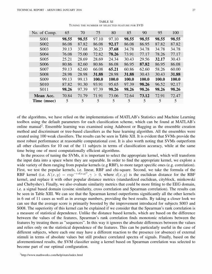
TECHNICAL REPORT - ARXIV.ORG JANUARY 2016 27
TABLE XITUNING THE NUMBER OF SELECTED FEATURE FOR SVD
No. of Comp. 65 70 75 80 85 90 95 100S001 98.55 98.55 97.10 97.10 98.55 98.55 98.55 98.55S002 86.08 87.82 86.08 92.17 86.08 86.95 87.82 87.82S003 39.13 37.68 36.23 37.68 34.78 34.78 34.78 34.78S004 76.08 75.00 72.82 78.26 73.91 77.17 78.26 77.17S005 25.21 28.69 28.69 24.34 30.43 29.56 32.17 30.43S006 80.86 82.60 80.86 86.08 86.95 87.82 86.95 86.08S007 59.13 62.60 66.08 65.21 60.86 62.60 58.26 60.00S008 28.98 28.98 31.88 28.98 31.88 30.43 30.43 31.88S009 99.13 99.13 100.0 100.0 100.0 100.0 100.0 100.0S010 87.82 91.30 93.91 95.65 97.39 98.26 96.52 92.17S011 98.26 97.39 97.39 98.26 98.26 98.26 98.26 98.26
Mean Acc. 70.84 71.79 71.91 73.06 72.64 73.12 72.91 72.47Time (msec) 5 5 5 5 5 5 5 5
of the algorithms, we have relied on the implementations of MATLAB’s Statistics and Machine Learningtoolbox using the default parameters for each classification scheme, which can be found at MATLAB’sonline manual2. Ensemble learning was examined using Adaboost or Bagging as the ensemble creationmethod and discriminant or tree-based classifiers as the base learning algorithm. All the ensembles werecreated using 100 weak classifiers. The results can be seen in Table XII. It is evident that SVMs provide themost robust performance at reasonable computational cost. It is also worth noting that SVMs outperformall other classifiers for 10 out of the 11 subjects in terms of classification accuracy, while at the sametime being one of most computationally efficient algorithms.
In the process of tuning the SVMs, it is important to select the appropriate kernel, which will transformthe input data into a space where they are separable. In order to find the appropriate kernel, we explore awide variety of them ranging from popular kernels (e.g RBF), to more target specific ones (e.g. correlation).First, we test the popular kernels, i.e. linear, RBF and chi-square. Second, we take the formula of theRBF kernel (i.e. K(x, y) = exp−γ·d(x,y)
2, γ > 0, where d(x, y) is the euclidean distance for the RBF
kernel, and replace it with other popular distance metrics (standardized euclidean, cityblock, minkowskiand Chebyshev). Finally, we also evaluate similarity metrics that could be more fitting to the EEG domain,i.e. a signal based domain (cosine similarity, cross correlation and Spearman correlation). The results canbe seen in Table XIII. We can see that the Spearman kernel outperforms significantly all the other kernelsin 6 out of 11 cases as well as in average numbers, providing the best results. By taking a closer look wecan see that the average score is primarily boosted by the improvement introduced for subjects S003 andS008. The superiority of this kernel can be explained if we consider that the Spearman’s rank correlation isa measure of statistical dependence. Unlike the distance based kernels, which are based on the differencebetween the values of the features, Spearman’s rank correlation finds monotonic relations between thefeatures by treating them as ”sequences”. In this way it ignores the absolute differences between the valuesand relies only on the statistical dependence of the features. This can be particularly useful in the case ofdifferent subjects, where each one may have a different reaction to the presence (or absence) of externalstimuli in terms of absolute values but still produce correlated spectra of signals. Finally, based on theaforementioned results, the SVM classifier using a kernel based on Spearman correlation was selected tobecome part of our optimal configuration.
2http://www.mathworks.com/help/stats/index.html
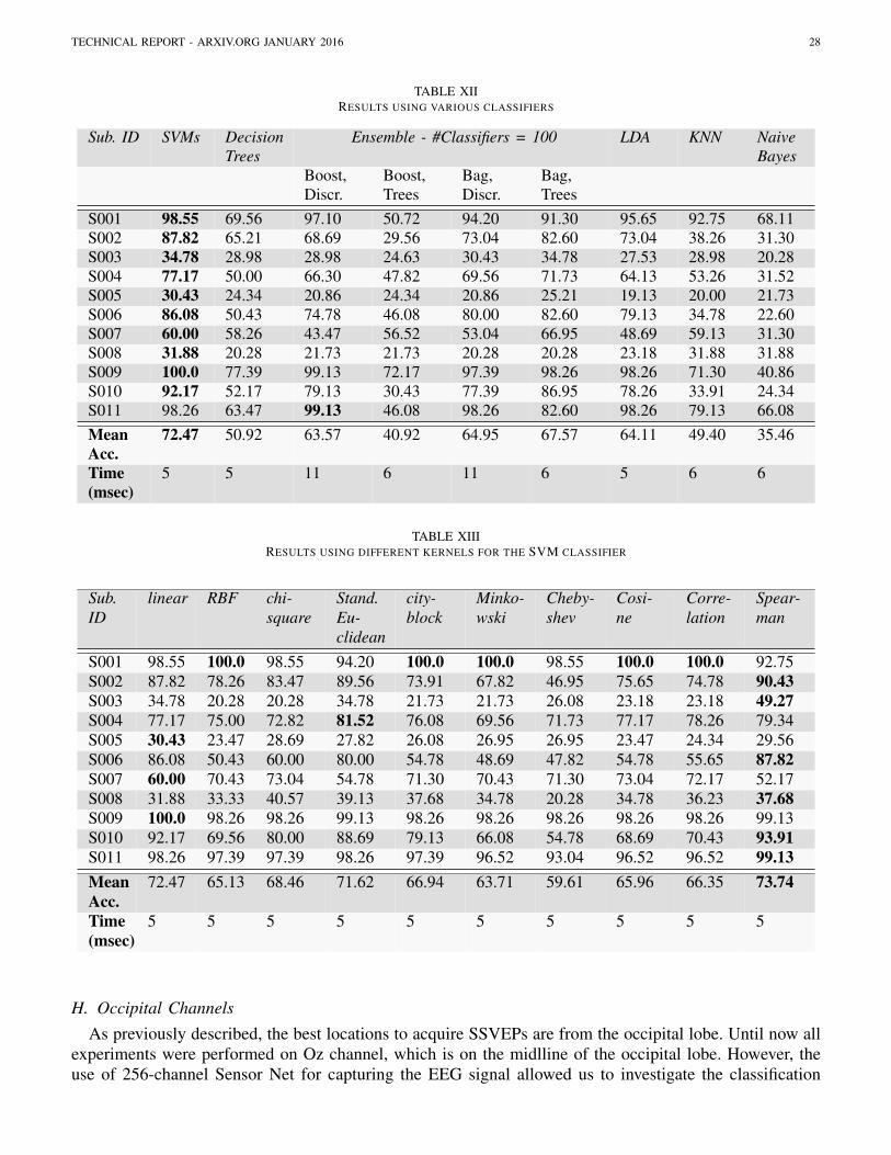
TECHNICAL REPORT - ARXIV.ORG JANUARY 2016 28
TABLE XIIRESULTS USING VARIOUS CLASSIFIERS
Sub. ID SVMs DecisionTrees
Ensemble - #Classifiers = 100 LDA KNN NaiveBayes
Boost,Discr.
Boost,Trees
Bag,Discr.
Bag,Trees
S001 98.55 69.56 97.10 50.72 94.20 91.30 95.65 92.75 68.11S002 87.82 65.21 68.69 29.56 73.04 82.60 73.04 38.26 31.30S003 34.78 28.98 28.98 24.63 30.43 34.78 27.53 28.98 20.28S004 77.17 50.00 66.30 47.82 69.56 71.73 64.13 53.26 31.52S005 30.43 24.34 20.86 24.34 20.86 25.21 19.13 20.00 21.73S006 86.08 50.43 74.78 46.08 80.00 82.60 79.13 34.78 22.60S007 60.00 58.26 43.47 56.52 53.04 66.95 48.69 59.13 31.30S008 31.88 20.28 21.73 21.73 20.28 20.28 23.18 31.88 31.88S009 100.0 77.39 99.13 72.17 97.39 98.26 98.26 71.30 40.86S010 92.17 52.17 79.13 30.43 77.39 86.95 78.26 33.91 24.34S011 98.26 63.47 99.13 46.08 98.26 82.60 98.26 79.13 66.08MeanAcc.
72.47 50.92 63.57 40.92 64.95 67.57 64.11 49.40 35.46
Time(msec)
5 5 11 6 11 6 5 6 6
TABLE XIIIRESULTS USING DIFFERENT KERNELS FOR THE SVM CLASSIFIER
Sub.ID
linear RBF chi-square
Stand.Eu-clidean
city-block
Minko-wski
Cheby-shev
Cosi-ne
Corre-lation
Spear-man
S001 98.55 100.0 98.55 94.20 100.0 100.0 98.55 100.0 100.0 92.75S002 87.82 78.26 83.47 89.56 73.91 67.82 46.95 75.65 74.78 90.43S003 34.78 20.28 20.28 34.78 21.73 21.73 26.08 23.18 23.18 49.27S004 77.17 75.00 72.82 81.52 76.08 69.56 71.73 77.17 78.26 79.34S005 30.43 23.47 28.69 27.82 26.08 26.95 26.95 23.47 24.34 29.56S006 86.08 50.43 60.00 80.00 54.78 48.69 47.82 54.78 55.65 87.82S007 60.00 70.43 73.04 54.78 71.30 70.43 71.30 73.04 72.17 52.17S008 31.88 33.33 40.57 39.13 37.68 34.78 20.28 34.78 36.23 37.68S009 100.0 98.26 98.26 99.13 98.26 98.26 98.26 98.26 98.26 99.13S010 92.17 69.56 80.00 88.69 79.13 66.08 54.78 68.69 70.43 93.91S011 98.26 97.39 97.39 98.26 97.39 96.52 93.04 96.52 96.52 99.13MeanAcc.
72.47 65.13 68.46 71.62 66.94 63.71 59.61 65.96 66.35 73.74
Time(msec)
5 5 5 5 5 5 5 5 5 5
H. Occipital ChannelsAs previously described, the best locations to acquire SSVEPs are from the occipital lobe. Until now all
experiments were performed on Oz channel, which is on the midlline of the occipital lobe. However, theuse of 256-channel Sensor Net for capturing the EEG signal allowed us to investigate the classification

TECHNICAL REPORT - ARXIV.ORG JANUARY 2016 29
Fig. 6. Mapping of the 256-channel Sensor Net and identification of the channels lying in the occipital are
performance in other parts of the brain that lie in the occipital area. Towards this goal, we used the mapof the 256-channel Sensor Net depicted in Figure 6 so as to identify the channels that lie in the occipitalarea. 40 channels were identified, which are the ones enclosed by the bounding boxes overlaid on themap of Figure 6.
After identifying the channels lying in the occipital area, the default configuration was used to estimatethe classification accuracy in each channel. The results are depicted in Table XIV. We can see that usingelectrode O2 results in better accuracy compared to Oz and that the use of O1 deteriorates significantlythe outcome. Furthermore, electrodes close to O2 seem to be more reliable, with channel-138 being thebest performing electrode with a mean accuracy of 74.42%, improved approximately by 2.0% comparedto the baseline configuration. In addition, we should mention that in the extended version of Table XIVwhere the accuracy is estimated per subject, it was particularly interesting to observe that the optimalelectrode varied per subject with a difference that could somehow reach (or exceed) 4% with respectto the default configuration. Finally, based on the results of Table XIV the EEG signals generated fromchannel 138 (see Figure 6) were used in our optimal configuration.
I. Optimal configurationBy combining the best performing algorithms and methods as indicated by the comparative evaluations
performed in Section VI we can obtain the optimal configuration of Table XV. We can see that there manydifferences compared to the default configuration of Table III, such as the incorporation of an IIR-ellipticfilter instead of an IIR-Chebyshev I, an artifact removal process based on AMUSE, a feature selectionalgorithm based on SVD, as well as the optimal tuning of PWelch for feature extraction and SVM forclassification. Finally, in the optimal configuration the EEG signals are obtained from channel-138 ratherthan channel-126 (see Figure 6).
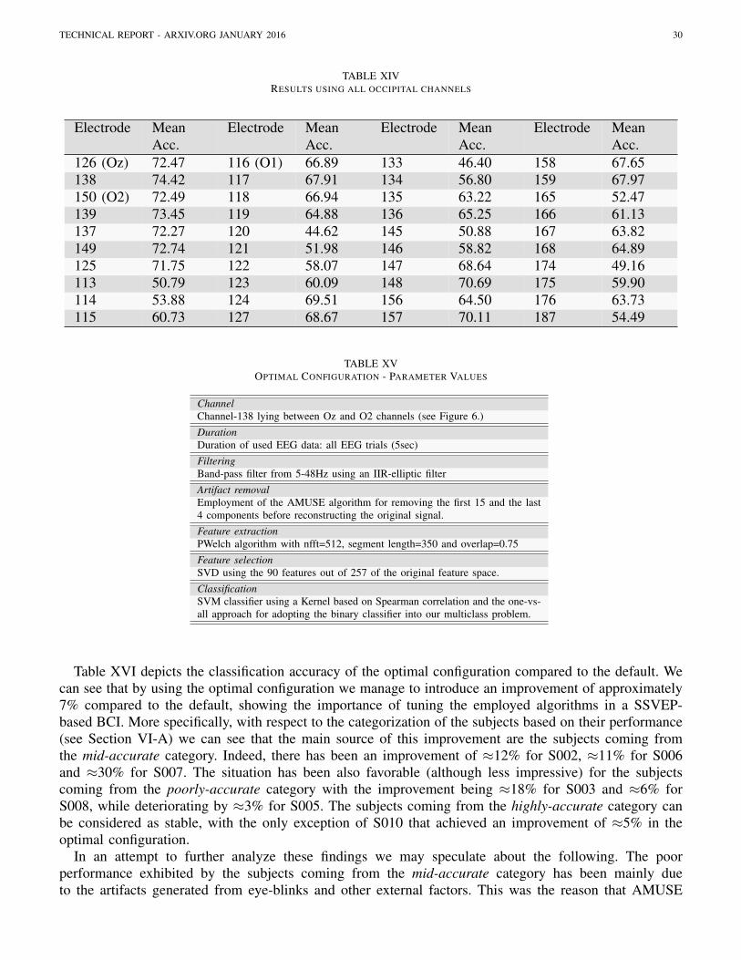
TECHNICAL REPORT - ARXIV.ORG JANUARY 2016 30
TABLE XIVRESULTS USING ALL OCCIPITAL CHANNELS
Electrode MeanAcc.
Electrode MeanAcc.
Electrode MeanAcc.
Electrode MeanAcc.
126 (Oz) 72.47 116 (O1) 66.89 133 46.40 158 67.65138 74.42 117 67.91 134 56.80 159 67.97150 (O2) 72.49 118 66.94 135 63.22 165 52.47139 73.45 119 64.88 136 65.25 166 61.13137 72.27 120 44.62 145 50.88 167 63.82149 72.74 121 51.98 146 58.82 168 64.89125 71.75 122 58.07 147 68.64 174 49.16113 50.79 123 60.09 148 70.69 175 59.90114 53.88 124 69.51 156 64.50 176 63.73115 60.73 127 68.67 157 70.11 187 54.49
TABLE XVOPTIMAL CONFIGURATION - PARAMETER VALUES
ChannelChannel-138 lying between Oz and O2 channels (see Figure 6.)DurationDuration of used EEG data: all EEG trials (5sec)FilteringBand-pass filter from 5-48Hz using an IIR-elliptic filterArtifact removalEmployment of the AMUSE algorithm for removing the first 15 and the last4 components before reconstructing the original signal.Feature extractionPWelch algorithm with nfft=512, segment length=350 and overlap=0.75Feature selectionSVD using the 90 features out of 257 of the original feature space.ClassificationSVM classifier using a Kernel based on Spearman correlation and the one-vs-all approach for adopting the binary classifier into our multiclass problem.
Table XVI depicts the classification accuracy of the optimal configuration compared to the default. Wecan see that by using the optimal configuration we manage to introduce an improvement of approximately7% compared to the default, showing the importance of tuning the employed algorithms in a SSVEP-based BCI. More specifically, with respect to the categorization of the subjects based on their performance(see Section VI-A) we can see that the main source of this improvement are the subjects coming fromthe mid-accurate category. Indeed, there has been an improvement of ≈12% for S002, ≈11% for S006and ≈30% for S007. The situation has been also favorable (although less impressive) for the subjectscoming from the poorly-accurate category with the improvement being ≈18% for S003 and ≈6% forS008, while deteriorating by ≈3% for S005. The subjects coming from the highly-accurate category canbe considered as stable, with the only exception of S010 that achieved an improvement of ≈5% in theoptimal configuration.
In an attempt to further analyze these findings we may speculate about the following. The poorperformance exhibited by the subjects coming from the mid-accurate category has been mainly dueto the artifacts generated from eye-blinks and other external factors. This was the reason that AMUSE

TECHNICAL REPORT - ARXIV.ORG JANUARY 2016 31
has been particularly effective in improving the performance for two of them (i.e. see S002 and S007 inTable VII). On the other hand, the very low performance of the subjects coming from the poorly-accuratecategory can be attributed to the failure of our system in capturing their EEG signals when reaching asteady-state, either due to problems in impedance (thick hair) or other reasons. In this case, particularlyfavorable has been the impact of employing the Spearman kernel (see S003 and S008 in Table XIII)indicating that a metric based on correlation can be more appropriate in these situations. Finally, the highperformance exhibited by the subjects coming from the highly-accurate category proved rather stableacross the different experiments.
Finally, we should note that the improved classification accuracy achieved with the optimal configurationcomes at the expense of additional computation cost. More specifically, the optimal configuration needs70 msecs to reach a decision, while the default configuration needs only 5 msecs. We can see that this ismainly due to the inclusion of the AMUSE method into the signal processing pipeline. However, a totalexecution time of 70 msecs for the signal processing module of a BCI system can still be considered asan acceptable delay for real-time applications.
TABLE XVICLASSIFICATION ACCURACY USING THE OPTIMAL CONFIGURATION.
Subject ID Default OptimalS001 98.5507 97.1014S002 87.8261 99.1304S003 34.7826 52.1739S004 77.1739 78.2609S005 30.4348 27.8261S006 86.0870 97.3913S007 60.0000 89.5652S008 31.8841 36.2319S009 100.000 100.000S010 92.1739 97.3913S011 98.2609 99.1304
Mean Acc. 72.4703 79.4729Time (msec) 5 70
VII. CONCLUSIONS AND OPPORTUNITIES FOR RESEARCH
It concluding this document it is interesting to highlight some of the areas that we consider as particularlyfavorable for future research based on our experimental findings. First and foremost it has been veryinteresting to observe the variability in the accuracy exhibited by the employed algorithms with respectto the examined subjects. More specifically, subjects S003, S005 and S008 (all classified in the poorlyaccurate category, see Section VI-A) were found to be the outliers in the superiority of the best performingalgorithms in many different cases. This diversity across subjects has been also observed for the optimallocation of the EEG electrodes. All the above, are clear evidence of the potential in devising “calibration”processes (e.g. running for a small period of time before the actual operation) that would allow the BCIsystem to optimally tune its internal parameters with respect to the particularity of the subject.
Another very interesting future direction that derives from the aforementioned observations is thepotential of fusing the information coming from different EEG channels in order to devise more robustclassification schemes. This type of approaches could either take the form of early fusion where the EEGsignals coming from different channels are combined before delivered to the classification scheme, or latefusion where an independent classifier is trained for each EEG channel and decisions are taken by jointlyconsidering the output of all classifiers, such as in a majority voting scheme.
Finally, another very important direction for future research has to do with the protocols employedfor communicating the visual stimuli and the information transfer rate achieved by the system. In ourexperiments, we have only investigated the most simple case where the subject is presented with a single

TECHNICAL REPORT - ARXIV.ORG JANUARY 2016 32
box flickering for 5 seconds and the feature extraction algorithm is applied on the full duration of thetrial. Although this setting allowed us to obtain very clean EEG signals and reach some very concreteconclusions about the optimal configuration of a BCI system, it can be considered prohibitive for a real-time application. Motivated by this fact our immediate plans for future work include the execution of anexperimental protocol where more than one visual stimuli are presented simultaneously to the subject, aswell as the investigation of the trade-off between the classification accuracy and the duration of the trial.
REFERENCES
[1] American Clinical Neurophysiology Society, “Guideline 9B: Recommended Standards for Visual Evoked Potentials.” https://www.acns.org/pdf/guidelines/Guideline-9B.pdf, 2008.
[2] S. Luck, An Introduction to the Event-Related Potential Technique. MIT Press, 2005.[3] C. Guger, A. Schlgl, C. Neuper, D. Walterspacher, T. Strein, and G. Pfurtscheller, “Rapid prototyping of an eeg-based brain-computer
interface (bci),” IEEE Trans. Neural Syst. Rehab. Eng., vol. 9, no. 1, p. 4958, 2001.[4] G. Pfurtscheller, R. Leeb, C. Keinrath, D. Friedman, C. Neuper, C. Guger, and M. Slater, “Walking from thought,” Brain Res., vol. 1071,
no. 1, p. 145152, 2006.[5] N. Hill, T. Lal, M. Schroder, T. Hinterberger, B. Wilhelm, F. Nijboer, U. Mochty, G. Widman, C. Elger, B. Scholkopf, A. Kubler, and
N. Birbaumer, “Classifying eeg and ecog signals without subject training for fast bci implementation: Comparison of nonparalyzed andcompletely paralyzed subjects,” IEEE Trans. Neural Syst. Rehab. Eng., vol. 14, p. 183186, 2006.
[6] N. Weiskopf, K. Mathiak, S. Bock, F. Scharnowski, R. Veit, W. Grodd, R. Goebel, and N. Birbaumer, “Principles of a brain-computerinterface (bci) based on real-time functional magnetic resonance imaging (fmri),” IEEE Trans. Biomed. Eng., vol. 51, p. 966970, 2004.
[7] S.-S. Yoo, T. Fairneny, N.-K. Chen, S.-E. Choo, L. Panych, H. Park, S.-Y. Lee, and F. Jolesz, “Brain-computer interface using fmri:Spatial navigation by thoughts,” Neuroreport, vol. 15, no. 10, p. 15911595, 2004.
[8] F. Matthews, B. Pearlmutter, T. Ward, C. Soraghan, and C. Markham, “Hemodynamics for brain-computer interfaces,” IEEE SignalProcessing Magazine, vol. 25, no. 1, pp. 87–94, 2008.
[9] G. Schalk, D. McFarland, T. Hinterberger, N. Birbaumer, and J. Wolpaw, “Bci2000: a general-purpose brain-computer interface (bci)system,” IEEE Transactions on Biomedical Engineering, vol. 51, pp. 1034–1043, June 2004.
[10] S. Amiri, A. Rabbi, L. Azinfar, and R. Fazel-Rezai, “A Review of P300, SSVEP, and Hybrid P300/SSVEP Brain- Computer InterfaceSystems,” in Brain-Computer Interface Systems - Recent Progress and Future Prospects (R. Fazel-Rezai, ed.), ch. 10, InTech, 2013.
[11] H.-T. Lin, C.-J. Lin, and R. C. Weng, “A note on platt’s probabilistic outputs for support vector machines,” Machine Learning, vol. 68,no. 3, pp. 267–276, 2007.
[12] S. N. Carvalho, T. B. Costa, L. F. Uribe, D. C. Soriano, G. F. Yared, L. C. Coradine, and R. Attux, “Comparative analysis of strategiesfor feature extraction and classification in SSVEP BCIs,” Biomedical Signal Processing and Control, vol. 21, pp. 34 – 42, 2015.
[13] H. Bakardjian, T. Tanaka, and A. Cichocki, “Optimization of SSVEP brain responses with application to eight-command braincomputer interface,” Neuroscience Letters, vol. 469, no. 1, pp. 34–38, 2010.
[14] X. Chen, Y. Wang, S. Gao, T.-P. Jung, and X. Gao, “Filter bank canonical correlation analysis for implementing a high-speed ssvep-basedbrain - computer interface,” Journal of Neural Engineering, vol. 12, no. 4, p. 046008, 2015.
[15] P. Martinez, H. Bakardjian, and A. Cichocki, “Fully online multicommand brain-computer interface with visual neurofeedback usingssvep paradigm,” Computational intelligence and neuroscience, vol. 2007, pp. 13–13, 2007.
[16] O. Friman, I. Volosyak, and A. Graser, “Multiple channel detection of steady-state visual evoked potentials for brain-computerinterfaces,” IEEE Transactions on Biomedical Engineering, vol. 54, pp. 742–750, April 2007.
[17] G. Garcia-Molina and D. Zhu, “Optimal spatial filtering for the steady state visual evoked potential: Bci application,” in 5th InternationalIEEE/EMBS Conference on Neural Engineering (NER), 2011, pp. 156–160, April 2011.
[18] S. Parini, L. Maggi, A. Turconi, and G. Andreoni, “A robust and self-paced bci system based on a four class ssvep paradigm: Algorithmsand protocols for a high-transfer-rate direct brain communication,” Intell. Neuroscience, pp. 2:1–2:11, Jan 2009.
[19] Y. Wang, R. Wang, X. Gao, B. Hong, and S. Gao, “A practical vep-based brain-computer interface,” IEEE Transactions on NeuralSystems and Rehabilitation Engineering, vol. 14, pp. 234–240, June 2006.
[20] P. Diez, V. Mut, E. A. Perona, and E. L. Leber, “Asynchronous bci control using high-frequency ssvep,” 2011.[21] A. Vilic, T. Kjaer., C. Thomsen., S. Puthusserypady, and H. Sorensen, “Dtu bci speller: An ssvep-based spelling system with dictionary
support,” in 35th Annual International Conference of the IEEE Engineering in Medicine and Biology Society (EMBC), 2013, pp. 2212–2215, 2013.
[22] G. R. Muller-Putz, R. Scherer, C. Brauneis, and G. Pfurtscheller, “Steady-state visual evoked potential (ssvep)-based communication:impact of harmonic frequency components,” Journal of Neural Engineering, vol. 2, no. 4, pp. 123–130, 2005.
[23] C. Jia, X. Gao, B. Hong, and S. Gao, “Frequency and phase mixed coding in ssvep-based brain–computer interface,” BiomedicalEngineering, IEEE Transactions on, vol. 58, pp. 200–206, Jan 2011.
[24] C. Guger, B. Allison, B. Grosswindhager, R. R. Pruckl, C. Hintermuller, C. Kapeller, M. Bruckner, G. Krausz, and G. Edlinger, “Howmany people could use an ssvep bci?,” Frontiers in Neuroscience, vol. 6, no. 169, 2012.
[25] S. N. Resalat and S. K. Setarehdan, “An improved ssvep based bci system using frequency domain feature classification,”[26] S. Rajesh and B. Haseena, “Comparison of ssvep signal classification techniques using svm and ann models for bci applications,”
International Journal of Information and Electronics Engineering, vol. 4, January 2014.[27] Y. Zhang, G. Zhou, J. Jin, M. Wang, X. Wang, and A. Cichocki, “L1-regularized multiway canonical correlation analysis for ssvep-based
bci,” IEEE Transactions on Neural Systems and Rehabilitation Engineering, vol. 21, pp. 887–896, Nov 2013.[28] Y. Zhang, J. Jin, X. Qing, B. Wang, and X. Wang, “Lasso based stimulus frequency recognition model for ssvep bcis,” Biomedical
Signal Processing and Control, vol. 7, no. 2, pp. 104 – 111, 2012.

TECHNICAL REPORT - ARXIV.ORG JANUARY 2016 33
[29] F. Lotte, M. Congedo, A. Lecuyer, F. Lamarche, and B. Arnaldi, “A review of classification algorithms for eeg-based brain - computerinterfaces,” Journal of Neural Engineering, vol. 4, no. 2, p. R1, 2007.
[30] A. V. Oppenheim, R. Schafer, and J. Buck, Discrete-time Signal Processing (2Nd Ed.). Prentice-Hall, Inc., 1999.[31] J. Proakis and D. Manolakis, Digital Signal Processing (3rd Ed.): Principles, Algorithms, and Applications. Prentice-Hall, Inc., 1996.[32] S. White, Digital Signal Processing: A Filtering Approach. Delmar Cengage Learning, 2000.[33] S. Choi, A. Cichocki, H.-M. Park, and S.-Y. Lee, “Blind Source Separation and Independent Component Analysis: A Review,” Neural
Information Processing - Letters and Reviews, vol. 6, pp. 1–57, jan 2005.[34] A. Hyvarinen and E. Oja, “Independent component analysis: Algorithms and applications,” Neural Networks, vol. 13, pp. 411–430,
2000.[35] T. Jung, S. Makeig, M. Mckeown, A. Bell, T. Lee, and T. Sejnowski, “Imaging brain dynamics using independent component analysis,”
Proc. IEEE, vol. 89, no. 7, 2001.[36] T. Jung, S. Makeig, M. Westerfield, J. Townsend, E. Courchesne, and T. Sejnowski, “Analysis and visualization of single-trial event-
related potentials,” Human Brain Mapping, vol. 14, pp. 166–185, 2001.[37] P. Stoica and R. Moses, Spectral Analysis of Signals. Pearson Prentice Hall, 2005.[38] S. Mallat, A Wavelet Tour of Signal Processing, Third Edition: The Sparse Way. Academic Press, 3rd ed., 2008.[39] C. Channon, “A mathematical theory of communication,” The Bell System Technical Journal, vol. 27, no. 7, pp. 379 – 423.[40] G. Brown, A. Pocock, M.-J. Zhao, and M. Lujan, “Conditional Likelihood Maximisation: A Unifying Framework for Information
Theoretic Feature Selection,” J. Mach. Learn. Res., vol. 13, pp. 27–66, Mar. 2012.[41] J. C. Platt, “Probabilistic outputs for support vector machines and comparisons to regularized likelihood methods,” in Advances in
Large Margin Classifiers, pp. 61–74, MIT Press, 1999.[42] “Geodesic EEG System 300.” https://www.egi.com/clinical-division/clinical-division-clinical-products/ges-300.[43] “Cedrus StimTracker.” http://cedrus.com/stimtracker/.[44] K. Georgiadis, G. Liaros, V. P. Oikonomou, E. Chatzilari, K. Adam, S. Nikolopoulos, and I. Kompatsiaris, “Mamem eeg ssvep dataset
i (256 channels, 11 subjects, 5 frequencies).” https://dx.doi.org/10.6084/m9.figshare.2068677.v1, 2016.[45] G. Liaros, V. P. Oikonomou, K. Georgiadis, E. Chatzilari, K. Adam, S. Nikolopoulos, and I. Kompatsiaris, “ssvep-eeg-processing-
toolbox.” https://github.com/MAMEM/ssvep-eeg-processing-toolbox, 2016.[46] C.-C. Chang and C.-J. Lin, “LIBSVM: A library for support vector machines,” ACM Transactions on Intelligent Systems and Technology,
vol. 2, pp. 27:1–27:27, 2011. Software available at http://www.csie.ntu.edu.tw/∼cjlin/libsvm.[47] C. Mssel, L. Lausser, M. Maucher, and H. Kestler, “Multi-objective parameter selection for classifiers,” Journal of Statistical Software,
vol. 46, no. 1, 2012.[48] S. Arlot and A. Celisse, “A survey of cross-validation procedures for model selection,” Statistics Surveys, vol. 4, pp. 40–79, 2010.[49] J. A. Rice and B. W. Silverman, “Estimating the mean and covariance structure nonparametrically when the data are curves,” Journal
of the Royal Statistical Society. Series B (Methodological), vol. 53, no. 1, pp. 233–243, 1991.[50] G. G. Xu and J. Huang, “Asymptotic optimality and efficient computation of the leave-subject-out cross-validation,” The Annals of
Statistics, vol. 40, pp. 3003–3030, 12 2012.[51] S. Fazli, F. Popescu, M. Danczy, B. Blankertz, K. Mller, and C. Grozea, “Subject-independent mental state classification in single
trials,” Neural Networks, vol. 22, pp. 1305–1312, 11 2009.