Mon. Not. R. Astron. Soc. 000, 1–15 (2015) Printed 7 June 2016 (MN LATEX style file v2.2)

A Herschel − SPIRE Survey of the Mon R2 Giant MolecularCloud: Analysis of the Gas Column Density Probability DensityFunction?

R. Pokhrel1†, R. Gutermuth1, B. Ali2, T. Megeath3, J. Pipher4, P. Myers5, W. J. Fischer6‡,T. Henning7, S. J. Wolk5, L. Allen8, J. J. Tobin91University of Massachusetts, Amherst, MA 01003, USA2Space Science Institute, Boulder, CO 80301, USA3University of Toledo, Toledo, OH 43606, USA4University of Rochester, Rochester, NY 14627, USA5CFA- Harvard University, Cambridge, MA 02138, USA6NASA’s Goddard Space Flight Center, Greenbelt, MD 20771, USA7MPIA- Heidelberg, Konigstuhl 17, 69117 Heidelberg, Germany8NOAO, Tucson, AZ 85719, USA9P.O. Box 9513, NL-2300 RA Leiden, The Netherlands

Accepted YEAR MONTH DAY. Received YEAR MONTH DAY; in original form YEAR MONTH DAY

ABSTRACTWe present a far-IR survey of the entire Mon R2 GMC with Herschel − SPIRE cross-calibrated with Planck−HFI data. We fit the SEDs of each pixel with a greybody functionand an optimal beta value of 1.8. We find that mid-range column densities obtained from far-IR dust emission and near-IR extinction are consistent. For the entire GMC, we find that thecolumn density histogram, or N-PDF, is lognormal below ∼1021 cm−2. Above this value, thedistribution takes a power law form with an index of -2.16. We analyze the gas geometry,N-PDF shape, and YSO content of a selection of subregions in the cloud. We find no regionswith pure lognormal N-PDFs. The regions with a combination of lognormal and one powerlaw N-PDF have a YSO cluster and a corresponding centrally concentrated gas clump. Theregions with a combination of lognormal and two power law N-PDF have significant numbersof typically younger YSOs but no prominent YSO cluster. These regions are composed ofan aggregate of closely spaced gas filaments with no concentrated dense gas clump. We findthat for our fixed scale regions, the YSO count roughly correlates with the N-PDF power lawindex. The correlation appears steeper for single power law regions relative to two power lawregions with a high column density cut-off, as a greater dense gas mass fraction is achieved inthe former. A stronger correlation is found between embedded YSO count and the dense gasmass among our regions.

Key words: ISM: individual objects (Mon R2) – ISM: clouds – ISM: structure

1 INTRODUCTION

Stars form within the dense regions of diffuse molecular clouds, butthe physical processes that determine the locations, rate, and effi-ciency of star formation are poorly understood. Based on prelim-inary results of the recent Herschel Gould Belt survey (HGBS),Andre et al. (2010) summarized the current picture of structure for-

? Herschel is an ESA space observatory with science instruments providedby European-led Principal Investigator consortia and with important partic-ipation from NASA.† E-MAIL: rpokhrel@astro.umass.edu‡ NASA Postdoctoral Program Fellow

mation in clouds as a two step process: first, a network of densefilaments are formed due to large-scale magneto-hydrodynamicturbulence, and then fragmentation occurs as gravity wins overturbulence thereby forming prestellar cores. The structure of thedense gas is affected by motions induced by supersonic turbulence(Padoan, Nordlund & Jones 1997), self-gravity of gas (Klessen,Heitsch & Mac Low 2000) and magnetic fields (Molina et al. 2012)inside the cloud. However, the role of each physical process instructure formation is still debated (McKee & Ostriker 2007).

Recent work suggests that aggregate column density diag-nostics, such as the column density probability distribution func-tion (N-PDF), which gives the probability of a region to have a

c© 2015 RAS

arX

iv:1

606.

0175

2v1

[as

tro-

ph.G

A]

6 J

un 2

016

2 Pokhrel et al.

column density within [N , N + dN ], are key to the identifica-tion of structure formation caused by different dominant physics(e.g., Kainulainen et al. 2009; Brunt, Federrath & Price 2010). Thecloud regions dominated by different physical phenomena exhibitN-PDFs of differing functional form. Aggregate N-PDFs of quies-cent clouds with very little star formation activity display a log-normal form, suggestive of structures formed by supersonic turbu-lence (Brunt, Federrath & Price 2010). Active star forming regionsexhibit some evidence of lognormal distribution at low densitiesas well, but also tend to have a power law excess from mediumto high column densities, where gas self gravity may be the dom-inant physics driving the cloud structure formation (Kainulainenet al. 2009). This mixed picture has been brought forward both byobservations (e.g., Hill et al. 2011) and theory (e.g., Padoan et al.2014), but only recently have datasets reached the degree of qualitynecessary to allow discriminating tests of this picture.

Among a few methods to map the distribution of column den-sities are mm-line emission features, extinction of background starsby dust, and thermal dust emission (c.f., Schnee et al. 2005). Thereare advantages and pitfalls to each process (Goodman, Pineda &Schnee 2009). For using line emission features, molecular trac-ers are mostly constrained by the optical depth effect of clouds,chemistry, and abundance variations more broadly. On the otherhand, the dust extinction suffers from selection effects as it de-pends on the detection of background stars. Thus, the lack of goodphotometry of weak stellar sources in high extinction regions canmake this process biased towards lower density regions. In con-trast, dust emission is free of these biases and allows us to makecolumn density maps with a very wide dynamic range. The adventof Herschel, with its unprecedented angular resolution and sensi-tivity in the far-IR, has enabled dust emission mapping of substan-tially greater quality than has been previously available over largeareas of sky (Andre et al. 2010).

Dust emission in the ISM is best modelled by an ensemble ofemitting particles that spans a substantial range of sizes, composi-tions, and temperatures (Draine 1978). For each line of sight, therecan be different emissivity properties for these emitting particles(dust grains) with different properties. Depending upon the avail-ability of data, different methods can be used to estimate emissivityfor each line of sight (Sadavoy et al. 2013). Recent efforts to es-timate column density, temperature, and dust emissivity generallyadopt a modified blackbody (greybody) model with wavelength de-pendent emissivity to represent the aggregate dust emission alongeach line of sight (e.g., Wood, Myers & Daugherty 1994).

In this work, we present an analysis of a new survey of theMon R2 giant molecular cloud (GMC) with Herschel- SPIRE.Our goal is to characterize the column density and temperaturestructure of the cloud, which is more distant, physically larger thanthe clouds in Gould’s Belt, and more actively forming stars. In §.1,we introduce the research with a literature review of Mon R2 GMC.In §.2, we explain our observations and data reduction procedurealong with an overview on the technique we implemented in un-derstanding the dust properties of Mon R2. We analyse the columndensity distribution in §.3. Finally, the conclusion of the paper issummarized in §.4.

1.1 Mon R2 Giant Molecular Cloud

The Mon R2 region was originally identified as a group of reflec-tion nebulae in the constellation of Monoceros. Seares & Hubble(1920) initially identified stars that may be exciting the nebulae andare responsible for the extended emission of the cloud. The first de-

tailed spectroscopic and photometric study of Mon R2 nebulae wasdone by Racine (1968) who discovered that the illuminating asso-ciated stars are mainly B-type stars. Racine (1968) estimated thedistance to the cloud as 830±50 pc which was later re-confirmedby Herbst & Racine (1976) by fitting the zero-age main sequencelocus from Johnson (1963) to dereddened UBV photometry.

Loren, Peters & Vanden Bout (1974) reported the first 12CO(J=1-0) detection in Mon R2 and Kutner & Tucker (1975) showedthat at least five of the reflection nebulae are associated with localmaxima in 12CO maps. The cloud was first mapped in its entiretyin 12CO by Maddalena et al. (1986) who surveyed ∼ 3◦ × 6◦ (44pc × 55 pc) region of the GMC. Peaks in molecular emission cor-responding to the location of reflection nebulae are traced by 13CO(Miesch, Scalo & Bally 1999). Xie (1992) estimated the mass 4 ×104 M� for the cloud using 12CO.

Carpenter (2000) used the 2MASS point source catalog toidentify compact stellar clusters, finding four clusters based on en-hancements in stellar surface density relative to the field star pop-ulation. These four clusters are associated with the Mon R2 core,GGD 12-15, GGD 17, and IRAS 06046-0603 as shown in figure 1.More recent works include the analysis of stellar distributions by K-band number counts and structure analysis, using near-IR data ob-tained with FLAMINGOS on the MMT and including SCUBA 850µm data (Gutermuth et al. 2005). Hodapp (2007) used the Wide-Field Camera on UKIRT in the 2.12 µm filter centered on the H2

1-0 S(1) emission line and discovered 15 H2 jets in Mon R2, con-firming most of the discoveries using archival Spitzer-IRAC 4.5and 8.0 µm. This work further asserted that the jets may be as-sociated with an episode of star formation in Mon R2 triggeredby the large central outflow. Further analysis by Gutermuth et al.(2011) reports a power law correlation with a slope 2.67 for theMon R2 cloud between the local surface densities of Spitzer iden-tified YSOs (∼ 1000) and the column density of gas as traced bynear-IR extinction.

2 DATA REDUCTION AND ANALYSIS

We surveyed the entire Mon R2 GMC with parallel scan-map modewith the ESA Herschel Space Observatory (Pilbratt et al. 2010)using both the Photoconductor Array Camera and Spectrometer,PACS, (Poglitsch et al. 2010) and the Spectral and PhotometricImaging REceiver, SPIRE, (Griffin et al. 2010). The target nameas designated in the Herschel Science Archive (HSA) is Mon R2-3 with corresponding OBSIDs 1342267715 and 1342267746. Forour analysis, we used only SPIRE data as we could not recoverlarge scale structure in the PACS 160 µm map reliably becauseit was found to be harshly contaminated. At large scales, PACS70 µm can not be used for studying extended emission. Herschelobserved Mon R2 on 15 March 2013 covering the area of 4.30◦ by4.36◦ and centered on 06h 08m 46.90s RA(J2000), - 06◦ 23′ 12.33′′

Dec(J2000) with position angle of 268.09◦. We obtained level-2SPIRE data products at 250 µm, 350 µm & 500 µm in both in-scan and cross-scan mode, i.e., in orthogonal scan directions to helpwith mitigation of scanning artifacts, at the scanning speed of 60′′

s−1. We reduced SPIRE observations using Herschel Interac-tive Processing Environment (HIPE) (Ott 2010), version 11.0.1.We adjusted standard pipeline scripts to construct combined mapsrecovering the extended emission from the two sets of scans.

We used Planck High Frequency Instrument (HFI) (PlanckHFI Core Team et al. 2011) maps to obtain an absolute calibra-tion for the SPIRE maps. Planck-HFI is a bolometric detector

c© 2015 RAS, MNRAS 000, 1–15

Mon R2 Herschel − SPIRE survey 3

Figure 1. False colour RGB image of the final set of SPIRE images whereB = 250 µm,G = 350 µm &R = 500 µm respectively, after calibrating withPlanck-HFI .

array designed to produce high sensitivity measurements coveringthe full sky in the wavelength range 0.3 to 3.6 mm. Herschel-SPIRE detectors are only sensitive to relative variations and ab-solute brightness can not be known but Planck-HFI sets an ab-solute offset to its maps. Both SPIRE and HFI share two chan-nels with overlapping wavebands. This is an advantage in calibrat-ing SPIRE maps (c.f., Bernard et al. 2010). We used PlanckHFI-545 and HFI-857 for this purpose, each with an angularresolution of 5′. We used the standard HIPE method to cali-brate Herschel maps. For this, HIPE convolves the SPIREmaps with the PLANCK beam in the area of interest and setsthe median SPIRE image flux level to be equal to the medianPLANCK level in the same area. All three SPIRE maps are ab-solute calibrated using the HFI emission to greybody conversionand colour correction for SPIRE assuming a greybody sourcespectrum, IS ∼ νβBν(T ) (see SPIRE handbook1 for details).For the SPIRE reduction, we applied relative gains, ran the de-striper in each band and then applied the zero-point correction us-ing the standard HIPE technique. Then we combined the finaldata for each bandpass into three mosaics used in the analysis dis-cussed below. The RGB image of these three wavebands are shownin figure 1.

The three bands in SPIRE have angular resolutions of 18′′,25′′ and 36′′. In order to fit a modified blackbody function to thedata from these images, we convolved the higher resolution im-ages with a 2D Gaussian kernel of an appropriate full width at halfmaximum (FWHM) to the resolution of the 500 µm data using therecipe from Aniano et al. (2011). It provides appropriate kernels formost of the space and ground based telescopes for the purpose ofmatching resolution in two sets of images. The convolved imageswere then regridded to 14′′ pixel size corresponding to SPIRE500 µm using the hastrom routine from the Interactive Data Lan-guage (IDL) Astronomy Users Library (Landsman 1993) so that a

1 http : //herschel.esac.esa.int/Docs/SPIRE/html/spire om.html

Figure 2. Flux vs. Error plot for SPIRE wavebands showing the actualflux values with their 1-σ uncertainties, presented in the form of a 2D his-togram. Synthetic lines for different SNR values are overplotted for eachwaveband.

given pixel position in each image corresponds to the same positionon the sky.

In figure 2, we present the resulting flux vs. uncertainty plotsfor all SPIRE bands as 2D histograms, with fiducial signal tonoise ratio (SNR) lines overplotted. The vast majority of our datahave high SNR. Our basis for the selection of high quality datapoints for subsequent analysis includes a requirement of SNR >10 in all three bands and good observing coverage based on theHSA-provided coverage maps.

2.1 Estimating dust properties

Cold dust emission in nearby molecular clouds is a thermal processand is generally modelled with a blackbody spectrum modified bya frequency-dependent emissivity (e.g., Hildebrand 1983). In gen-

c© 2015 RAS, MNRAS 000, 1–15

4 Pokhrel et al.

eral, the radiative transfer equation governing the emission Iν for amodified blackbody spectrum is:

Iν = Bν(T )× (1− e−τν ) + Ibackν e−τν + I foreν (1)

where Bν(T ) is the Planck function for a perfect blackbodyof temperature T in Kelvin and τν is the opacity of the cloud atcorresponding frequency ν. Equation 1 for the optically thin casetakes the form:

Iν = Bν(T )× τν + Icomν (2)

where Icomν is the combined foreground and background emis-sion which can be neglected in our case due to the position of thecloud, several degrees away from the Galactic plane. Since, τν =κν Σ; Σ being the mass surface density and κν ∝ νβ where β isthe dust emissivity power law index, equation 2 takes the followingform:

Iν = κν0(ν/ν0)βBν(T )Σ (3)

where κν0 is a reference dust opacity per unit gas and dustmass at a reference frequency ν0. We took κν0 = 2.90 cm2/gm forν0 corresponding to the longest observed wavelength, 500 µm, fol-lowing the OH-4 model (Mathis, Rumpl & Nordsieck (1977) dis-tribution for dust grains in the ISM: f(a) ∝ a−3.5, with thin icemantles on dust grains and no coagulation) from Ossenkopf & Hen-ning (1994). T is the dust temperature and Σ = µmHN(H2) whereµ is the mean molecular weight per unit hydrogen mass ∼ 2.8 fora cloud with 71% molecular hydrogen, 27% helium and 2% met-als (Sadavoy et al. 2013), mH is the mass of single hydrogen atomand N(H2) is the gas column density. Hence, we are observing thedust emission and using it as a probe to compute the gas columndensity. We assume the canonical gas-to-dust ratio of 100 (Predehl& Schmitt 1995) for our purpose.

2.1.1 Dust spectral index, β

Our goal is to fit the spectral energy distribution (SED) of individ-ual pixels with equation 3. Since we could not rely on the PACSdata, it limited the available data to three SPIRE wavebands only.This led to the problem of fitting the observations with three datapoints with an equation of three unknowns. Andre et al. (2010), Sa-davoy et al. (2012) and Arzoumanian et al. (2011) assume β to bea constant between 1.5 (hotter regions) and 2 (colder regions). Weused the SPIRE flux ratios to estimate the most appropriate valueof β so that it best represents the whole cloud complex.

In Figure 3 we plot the ratio of fluxes between 250 µm and 350µm on the x-axis and the ratio of fluxes between 350 µm and 500µm on the y-axis. Equation 3 is used to compute the reference fluxratios at different wavebands for a given choice of β and tempera-ture. To our benefit, the column density and emissivity calibrationconstant cancel in this ratio-space. For frequencies ν1 and ν2, theequation reduces to a simple form:

Iν1Iν2

=

(ν1ν2

)βBν1(T )

Bν2(T )(4)

We used equation 4 to plot the flux ratio for SPIRE wave-bands for different β and temperatures, as shown in figure 3. Wefound that the colder region seems to peak at β ∼ 2 and the warm

Figure 3. F250/F350 Vs. F350/F500 plot as a 2D histogram, overlaid withtheoretical greybody plots for different β and temperature ranges, showingunique values for both β and temperature for each pixel. The data are bestmatched across the entire space with β = 1.8. The black cross in the plotrepresents the typical error, which is the median error of the overall distri-bution of flux ratio points.

regions are more accurately defined by β ∼ 1.6, giving a value ofβ ∼ 1.8 as an intermediate value that can be used to explain thewhole cloud. We have bracketed the extremes of the data with βof 1.0 and 2.5 models. The black error cross represents the typicalflux ratio uncertainty derived from the errors in each flux as 1-σuncertainty.

The correct estimation of β is crucial because the greybody fitcalculations for a different value of β can give a different estimationof temperature and column density. Thus we tested the effect of theβ uncertainty on the physical measurements that we derive from thedata. Figure 4 shows the distribution of N(H2) and the temperaturefor β = 1.8. It also includes the possible fluctuation of β from 1.8 to1.5 (hotter regions) or 2.0 (colder regions). We found that the valuesshift by 30% in those cases, relative to the values derived using β= 1.8. The plot also shows that if we choose a higher (or lower)β values, we will be over-determining (or under-determining) thecolumn density and under-determining (or over-determining) thetemperature.

2.2 Modified blackbody fits

After fixing β to 1.8, we fitted the SED for each pixel position us-ing the PYTHON program curvefit which finds the best fittingparameter values for a particular model by doing an iterative least-squares comparison between data and the theoretical model. 1-σflux uncertainty values for each data point are accessible from thedata archival pipeline. Thus, we obtained the temperature and col-umn density maps with 1-σ uncertainties in each. The temperatureis distributed between 11 K and 43 K and the N(H2) vary between3 × 1020 cm−2 and 9 × 1022 cm−2. The uncertainty in the canon-ical gas-to-dust ratio is ∼30% and figure 4 shows the typical un-certainty in the selection of β as ∼30%. Similarly, the propagateduncertainties in N(H2) and the temperature values when best fittedare between 0.1% and 5%. This gives the overall error in the es-timation of final N(H2) and temperature values to be ∼40%. Themass-weighted mean temperature is ∼ 17 K. We calculated the to-tal mass of the GMC to be 4× 104 M�, which is calculated over 2

c© 2015 RAS, MNRAS 000, 1–15

Mon R2 Herschel − SPIRE survey 5

Figure 4. Column density and temperature distributions in Mon R2 aftergreybody fitting, for different β values.

× 103 pc2 projected area. This mass estimate is similar to the valuepreviously calculated by Xie (1992).

Figure 5 shows the temperature-column density map. Columndensity in the map is shown in terms of intensity and temperatureis shown by colour, where the redder areas are colder (<10 K) andbluer areas are hotter (>20 K). Just upon visual inspection, themap clearly shows a variety of structures from diffuse regions tofilaments and clumps. We can see variation in structures, from sub-parsec scales to tens of parsec scales. Some of the structures resem-ble elongated filaments whereas some resemble relatively roundclumps, with varying column density contrast. Multiple filamentscan be seen radiating towards the central Mon R2 clump forminghub-spoke like structure (Myers 2009). Also filaments seem to beassociated with GGD 12-15 and other clumps (c.f. figure 1).

2.3 Rayleigh-Jeans limitation

Being limited to the SPIRE wavebands, our temperature dynamicrange is more constrained on the high end than some comparableHerschel surveys (Andre et al. 2010). Here, we explore the pixelsfor which the SED lies in the Rayleigh-Jeans (R-J) tail of the grey-body spectrum. We use equation 3 to reliably estimate the tempera-ture and column density for the data points for which the deviationin fluxes is sufficient enough to constrain the peak of the SED. Forthe points where the SPIRE bands fall on the R-J tail, equation3 can not give a reliable estimate of the parameters. Hence, here

Figure 5. Temperature-Column density map of Mon R2 obtained after per-forming modified blackbody fits to the SPIRE data. Intensity is mappedas column density and colour is mapped as temperature where the redderareas are colder (<10 K) and bluer areas are hotter (>20 K). The typicaltemperature of the dust is ∼ 17 K.

we examined the region of colour-colour space where the SPIREdata would indicate that they are on the R-J regime of the SED.

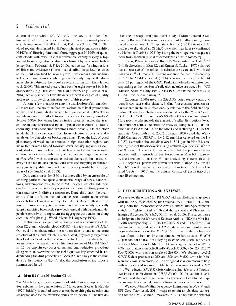
In figure 3, we show the loci of colours for SPIRE data inthe limit that the temperatures are high enough that they fall on theR-J tail. Figure 3 represents a 2D histogram of actual flux ratios andthe grey dashed line represents the R-J locus. The typical 1σ uncer-tainty in flux ratios is represented by a black error cross on the plot,though we note that the flux ratio uncertainties vary substantiallyamong pixels. To gauge the R-J locus proximity for each pixel, wecalculated the distance to the nearest R-J point in units of sigma(cf. figure 3) and plotted them with the temperature for each pixel.Figure 6 shows the histogram of the number of sigmas required toreach the nearest point on the R-J locus and a plot of temperaturewith those number of sigmas. The vast majority of pixels have alarge number of sigma. The high temperature pixels mostly havelow number of sigma implying a higher probability of being R-Jlimited.

We want to estimate the temperature threshold where theemission could be warm enough to be consistent with an R-J spec-trum through the SPIRE bands. For this, we binned the pixels bytemperature and calculated the fraction of pixels less than a givennumber of sigma away from the R-J locus for each bin (see Figure7). Pixels found to be less than a few sigma have a non-negligibleprobability of being consistent with an R-J limited SED, and thusmay lack an upper boundary on their temperature estimate. Thus tominimize such unconstrained fits, we picked only those pixels forwhich the number of sigma is greater than 5 and temperature<28 Kfor studying the column density distribution (§.3). There are ∼500pixels out of 105 that do not meet these requirements. We foundthat their exclusion doesn’t significantly change the shape of the N-PDF of the whole cloud (figure 9), nor of the affected subregions(§. 3.2 and figure 13).

c© 2015 RAS, MNRAS 000, 1–15

6 Pokhrel et al.

Figure 6. The top panel shows the distribution of the number of sigma awayfrom the R-J locus. Smaller numbers of sigma represent the points whichare closer to the R-J locus and may be consistent with an R-J SED. Largernumbers of sigma represent those that are clearly distinct from the R-J limitand thus are more reliably explained by the greybody emission. We over-plotted another histogram for T > 28 K which shows that these are thepixels with low number of sigmas. The bottom panel is a 2D histogram ofthe number of sigma for each pixel versus its greybody fit temperature.

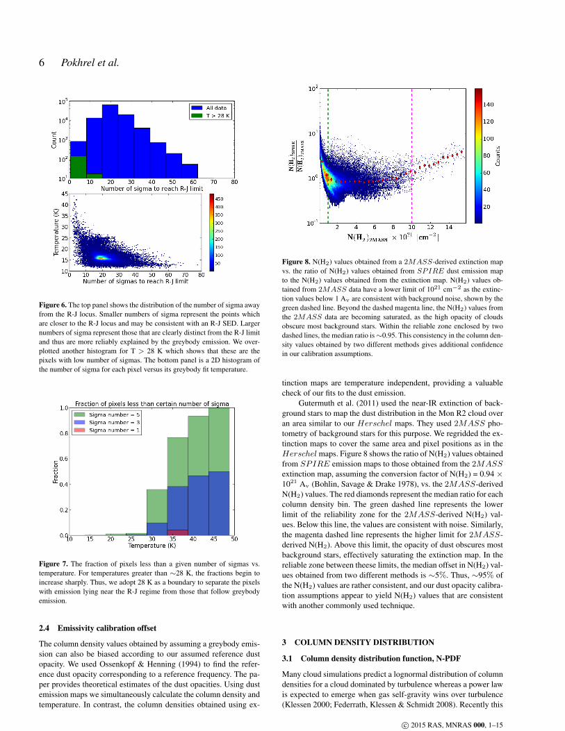
Figure 7. The fraction of pixels less than a given number of sigmas vs.temperature. For temperatures greater than ∼28 K, the fractions begin toincrease sharply. Thus, we adopt 28 K as a boundary to separate the pixelswith emission lying near the R-J regime from those that follow greybodyemission.

2.4 Emissivity calibration offset

The column density values obtained by assuming a greybody emis-sion can also be biased according to our assumed reference dustopacity. We used Ossenkopf & Henning (1994) to find the refer-ence dust opacity corresponding to a reference frequency. The pa-per provides theoretical estimates of the dust opacities. Using dustemission maps we simultaneously calculate the column density andtemperature. In contrast, the column densities obtained using ex-

Figure 8. N(H2) values obtained from a 2MASS-derived extinction mapvs. the ratio of N(H2) values obtained from SPIRE dust emission mapto the N(H2) values obtained from the extinction map. N(H2) values ob-tained from 2MASS data have a lower limit of 1021 cm−2 as the extinc-tion values below 1 Av are consistent with background noise, shown by thegreen dashed line. Beyond the dashed magenta line, the N(H2) values fromthe 2MASS data are becoming saturated, as the high opacity of cloudsobscure most background stars. Within the reliable zone enclosed by twodashed lines, the median ratio is∼0.95. This consistency in the column den-sity values obtained by two different methods gives additional confidencein our calibration assumptions.

tinction maps are temperature independent, providing a valuablecheck of our fits to the dust emission.

Gutermuth et al. (2011) used the near-IR extinction of back-ground stars to map the dust distribution in the Mon R2 cloud overan area similar to our Herschel maps. They used 2MASS pho-tometry of background stars for this purpose. We regridded the ex-tinction maps to cover the same area and pixel positions as in theHerschelmaps. Figure 8 shows the ratio of N(H2) values obtainedfrom SPIRE emission maps to those obtained from the 2MASSextinction map, assuming the conversion factor of N(H2) = 0.94 ×1021 Av (Bohlin, Savage & Drake 1978), vs. the 2MASS-derivedN(H2) values. The red diamonds represent the median ratio for eachcolumn density bin. The green dashed line represents the lowerlimit of the reliability zone for the 2MASS-derived N(H2) val-ues. Below this line, the values are consistent with noise. Similarly,the magenta dashed line represents the higher limit for 2MASS-derived N(H2). Above this limit, the opacity of dust obscures mostbackground stars, effectively saturating the extinction map. In thereliable zone between theese limits, the median offset in N(H2) val-ues obtained from two different methods is ∼5%. Thus, ∼95% ofthe N(H2) values are rather consistent, and our dust opacity calibra-tion assumptions appear to yield N(H2) values that are consistentwith another commonly used technique.

3 COLUMN DENSITY DISTRIBUTION

3.1 Column density distribution function, N-PDF

Many cloud simulations predict a lognormal distribution of columndensities for a cloud dominated by turbulence whereas a power lawis expected to emerge when gas self-gravity wins over turbulence(Klessen 2000; Federrath, Klessen & Schmidt 2008). Recently this

c© 2015 RAS, MNRAS 000, 1–15

Mon R2 Herschel − SPIRE survey 7

Figure 9. The N-PDF of the entire Mon R2 GMC. A lognormal distributionis seen for Log N(H2) < (21.041 ± 0.001) cm−2 pertaining to the regiondominated by supersonic turbulence. A power law nature is seen for valuesgreater than this value with a power law index (-2.158 ± 0.002) pertainingto the regions dominated by self-gravity of gas. The y-axis represents thelog of the number of 14′′ × 14′′ pixels.

has been simulated and studied by Lee, Chang & Murray (2014).These two different natures of the probability distribution function(PDF) have been commonly observed. However, Kritsuk, Norman& Wagner (2011) recently put forward the idea that the power lawnature is due to regions that collapse under self-gravity and thedensity profiles of collapsing regions determine the power law ex-ponent. Lee, Chang & Murray (2014) checked this suggestion byplotting the PDF of the regions undergoing gravitational collapse,regions largely unaffected by the gravity of the stars, and the entiresimulation region before and after turning on the gas self-gravity.In their simulation, a star refers to the sink particle which is formedat a grid point at which the Jeans length falls below four grid cells(Truelove et al. 1997). They found that the density PDF of the non-collapsing regions matches the PDF of the entire region before in-clusion of gravity. In other words, the PDF was lognormal withouta power law tail at high densities. The implication was that regionsthat do not undergo collapse retain the character of pure supersonicturbulence whereas the density PDFs of collapsing regions developa clear power law at high density. The importance of self-gravitywas realised by considering several scenarios of gravitational in-teraction in the molecular cloud: self-gravity of gas on gas, self-gravity of stars on stars and the gravity between gas and stars. Lee,Chang & Murray (2014) demonstrated that the gravity due to starsdoes not have a significant effect on the star formation rate and gasself-gravity is the only dominant mechanism.

While N-PDFs have been recognized as a powerful analysistool, it is important to note that the observed shapes of N-PDFs canbe impacted by effects other than gas physics. Beam smoothing ofcomplex projected gas geometries are the largest potential concern.In particular, small, closely spaced, high density features embed-ded within lower density surroundings that are smoothed by a largebeam can result in substantial shifting of low density pixels upwardand high density pixels downward. Generally, the reduction of thedensities of the less numerous high column density pixels will havea stronger impact on the high column density portion of the N-PDF.Our high data quality and emphasis on relative differences in theregional N-PDF of one cloud should minimize the impact of theseeffects on our broader analysis, however.

Figure 10. Example plots of MCMC convergence verification. Upper left:Fluctuation of the best fitted slope in later iterations. The range of fluctu-ation is very small. Lower left: Autocorrelation degree of best fitted slopevalues. In a longer time gap, the autocorrelation goes to zero showing thatthe initial and final parameter values are not related. Right: Histogram ofthe best fitted slope values with the peak value marked by a dark black line.Black dotted lines represent the values within a 1-σ limit.

Given the ongoing star formation in the MonR2 cloud, we ex-pected to see both components, i.e., self-gravitating structures em-bedded within a larger, diffuse, turbulent region within a given pro-jected region (Kainulainen et al. 2009). However, along with thesetwo possibilities of a pure lognormal function and a combinationof a lognormal and a power law function model, we found it neces-sary to consider a third model. Upon carefully studying the columndensity distributions of several subregions (see §3.2, below), thecolumn density distributions of some seem to have two power lawsinstead of just one. The possibility of two power laws has been re-ported recently in other studies as well (Schneider et al. 2015a).Hence, we considered the possibility of a third model with a log-normal and two power law components.

With different possibile models for the nature of an N-PDF,we generalized our fitting process to fit for the three differentempirical scenarios, a lognormal function with zero to two powerlaws at higher column densities. If p(x) is the probability distri-bution function, we fit the N-PDF for the whole region as well asfor selected subregions (§3.2) using the following different models:

For the pure lognormal:

pG(x) = Log

[A exp

(− (x− x0)2

2σ2

)](5)

where x = log(N ), N is the column density. A is the peak, x0 isthe mean and σ is the standard deviation of the distribution in logunits. We have taken the log of the lognormal function because weare fitting logarithmic data (cf. figure 9).

For the combination of a lognormal with one power law:

pG+1(x) =

{pG(x), if x 6 xbrk1

α1x+ pG(xbrk1), if x > xbrk1(6)

xbrk1 is the value of log(N ) after which the distribution takespower law form. This value is determined by the fitter itself byusing it as a free parameter. The fitter is designed to look for twodifferent subsets of data with a breaking point and fits them withthe above function, considering every N value in the sample spaceas the breaking point. Finally xbrk1 is selected by optimizing theleast squares for each of the considered data. α1 is the index of

c© 2015 RAS, MNRAS 000, 1–15

8 Pokhrel et al.

the power law. The y-intercept is constrained so that the power lawfunction is continuous with the lognormal.

For the combination of a lognormal with two power laws:

pG+2(x) =

pG(x), if x 6 xbrk1

α1x+ pG(xbrk1), if xbrk1 < x 6 xbrk2

α2x+ pG+1(xbrk2), if x > xbrk2

(7)

Similarly, xbrk2 is the value of log(N ) from where the secondpower law (of index α2 develops. These values are also used asfree parameters so that we can be unbiased in our selection of thebreaking points.

We used a Monte Carlo analysis to estimate the uncertaintiesin each bin. We randomly sampled column density values assumingthat the uncertainty in column density follows a Gaussian distribu-tion. The spread in the values for each bin gives 1-σ uncertainty forthat particular bin. We have 7 free parameters in our models andthe models themselves are the combination of different functions.Hence, we need a robust fitter that can give the best fitting valuesfrom the parameter space along with reliable uncertainties. For this,we used the Markov Chain Monte Carlo (MCMC) method (vanDyk 2003). We have followed the Metropolis-Hastings algorithm inwhich the samples are selected from an arbitrary “proposal” distri-bution. These samples are kept or discarded according to the accep-tance rule. The whole process is repeated until we get a “transition”probability function so that the algorithm can transit from one setof parameter values to a more probable set. Based on the transitionprobability where the current point depends only on the previouspoint but yet can still span over the whole parameter space, an er-godic chain of positions in parameter space is formed, known asthe Markov Chain. The Markov Chain samples from the posteriordistribution ergodically assuming the detailed balance condition.MCMC estimates the expectation of a statistic in a complex modelby doing simulations that randomly select from a Markov Chain.We have used the PYTHON package Pymc for this purpose (Patil,Huard & Fonnesbeck 2010).

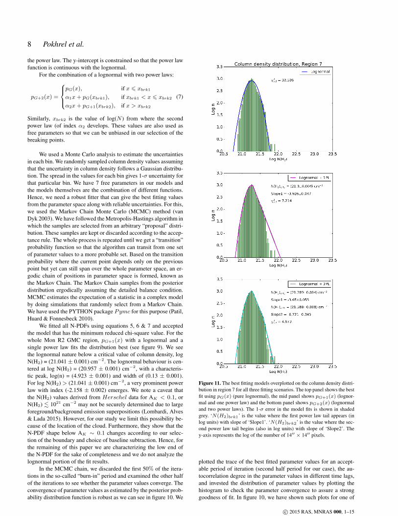
We fitted all N-PDFs using equations 5, 6 & 7 and acceptedthe model that has the minimum reduced chi-square value. For thewhole Mon R2 GMC region, pG+1(x) with a lognormal and asingle power law fits the distribution best (see figure 9). We seethe lognormal nature below a critical value of column density, logN(H2) = (21.041 ± 0.001) cm−2. The lognormal behaviour is cen-tered at log N(H2) = (20.957 ± 0.001) cm−2, with a characteris-tic peak, log(n) = (4.923 ± 0.001) and width of (0.13 ± 0.001).For log N(H2) > (21.041 ± 0.001) cm−2, a very prominent powerlaw with index (-2.158 ± 0.002) emerges. We note a caveat thatthe N(H2) values derived from Herschel data for AK < 0.1, orN(H2) . 1021 cm−2 may not be securely determined due to largeforeground/background emission superpositions (Lombardi, Alves& Lada 2015). However, for our study we limit this possibility be-cause of the location of the cloud. Furthermore, they show that theN-PDF shape below AK ∼ 0.1 changes according to our selec-tion of the boundary and choice of baseline subtraction. Hence, forthe remaining of this paper we are characterizing the low end ofthe N-PDF for the sake of completeness and we do not analyze thelognormal portion of the fit results.

In the MCMC chain, we discarded the first 50% of the itera-tions in the so-called “burn-in” period and examined the other halfof the iterations to see whether the parameter values converge. Theconvergence of parameter values as estimated by the posterior prob-ability distribution function is robust as we can see in figure 10. We

Figure 11. The best fitting models overplotted on the column density distri-bution in region 7 for all three fitting scenarios. The top panel shows the bestfit using pG(x) (pure lognormal), the mid panel shows pG+1(x) (lognor-mal and one power law) and the bottom panel shows pG+2(x) (lognormaland two power laws). The 1-σ error in the model fits is shown in shadedgrey. ‘N(H2)brk1’ is the value where the first power law tail appears (inlog units) with slope of ‘Slope1’. ‘N(H2)brk2’ is the value where the sec-ond power law tail begins (also in log units) with slope of ‘Slope2’. They-axis represents the log of the number of 14′′ × 14′′ pixels.

plotted the trace of the best fitted parameter values for an accept-able period of iteration (second half period for our case), the au-tocorrelation degree in the parameter values in different time lags,and invested the distribution of parameter values by plotting thehistogram to check the parameter convergence to assure a stronggoodness of fit. In figure 10, we have shown such plots for one of

c© 2015 RAS, MNRAS 000, 1–15

Mon R2 Herschel − SPIRE survey 9

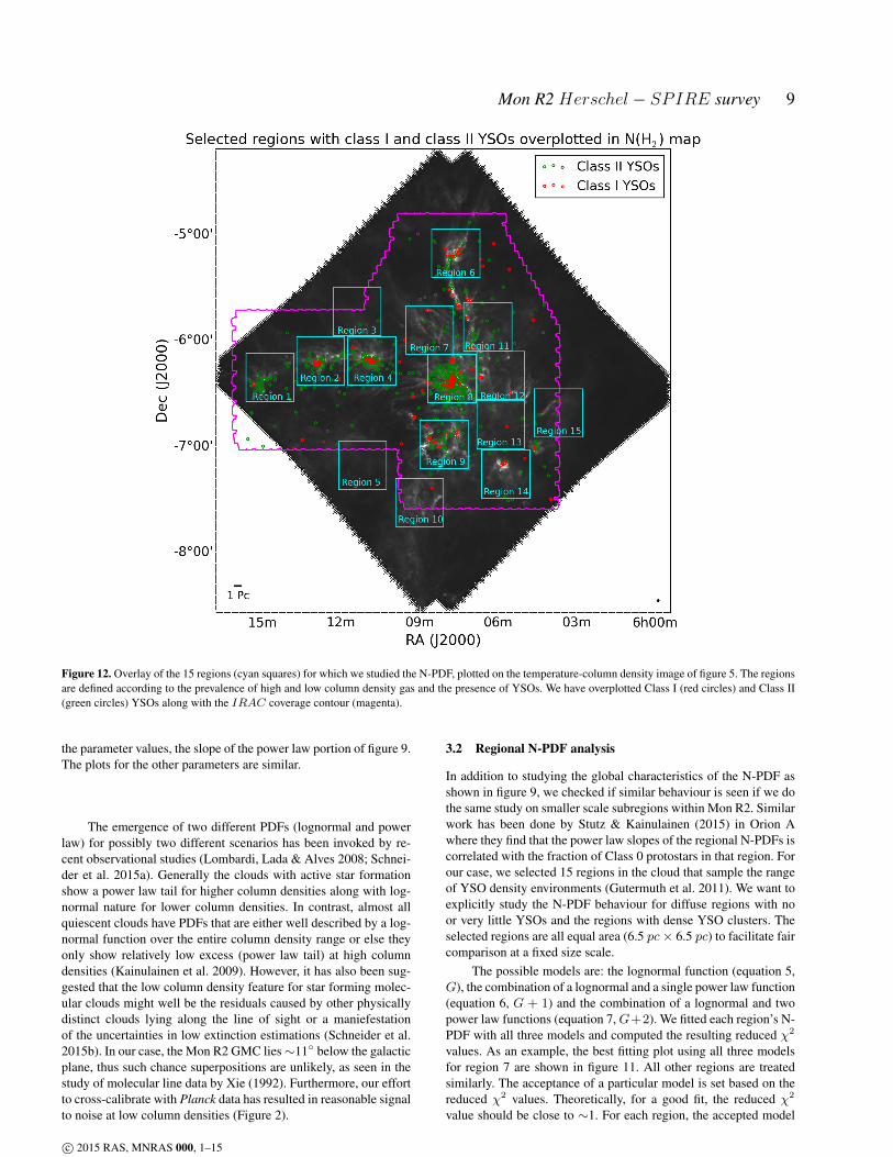
Figure 12. Overlay of the 15 regions (cyan squares) for which we studied the N-PDF, plotted on the temperature-column density image of figure 5. The regionsare defined according to the prevalence of high and low column density gas and the presence of YSOs. We have overplotted Class I (red circles) and Class II(green circles) YSOs along with the IRAC coverage contour (magenta).

the parameter values, the slope of the power law portion of figure 9.The plots for the other parameters are similar.

The emergence of two different PDFs (lognormal and powerlaw) for possibly two different scenarios has been invoked by re-cent observational studies (Lombardi, Lada & Alves 2008; Schnei-der et al. 2015a). Generally the clouds with active star formationshow a power law tail for higher column densities along with log-normal nature for lower column densities. In contrast, almost allquiescent clouds have PDFs that are either well described by a log-normal function over the entire column density range or else theyonly show relatively low excess (power law tail) at high columndensities (Kainulainen et al. 2009). However, it has also been sug-gested that the low column density feature for star forming molec-ular clouds might well be the residuals caused by other physicallydistinct clouds lying along the line of sight or a maniefestationof the uncertainties in low extinction estimations (Schneider et al.2015b). In our case, the Mon R2 GMC lies∼11◦ below the galacticplane, thus such chance superpositions are unlikely, as seen in thestudy of molecular line data by Xie (1992). Furthermore, our effortto cross-calibrate with Planck data has resulted in reasonable signalto noise at low column densities (Figure 2).

3.2 Regional N-PDF analysis

In addition to studying the global characteristics of the N-PDF asshown in figure 9, we checked if similar behaviour is seen if we dothe same study on smaller scale subregions within Mon R2. Similarwork has been done by Stutz & Kainulainen (2015) in Orion Awhere they find that the power law slopes of the regional N-PDFs iscorrelated with the fraction of Class 0 protostars in that region. Forour case, we selected 15 regions in the cloud that sample the rangeof YSO density environments (Gutermuth et al. 2011). We want toexplicitly study the N-PDF behaviour for diffuse regions with noor very little YSOs and the regions with dense YSO clusters. Theselected regions are all equal area (6.5 pc× 6.5 pc) to facilitate faircomparison at a fixed size scale.

The possible models are: the lognormal function (equation 5,G), the combination of a lognormal and a single power law function(equation 6, G + 1) and the combination of a lognormal and twopower law functions (equation 7,G+2). We fitted each region’s N-PDF with all three models and computed the resulting reduced χ2

values. As an example, the best fitting plot using all three modelsfor region 7 are shown in figure 11. All other regions are treatedsimilarly. The acceptance of a particular model is set based on thereduced χ2 values. Theoretically, for a good fit, the reduced χ2

value should be close to ∼1. For each region, the accepted model

c© 2015 RAS, MNRAS 000, 1–15

10 Pokhrel et al.

Figure 13. The accepted models (c.f. table 1) overplotted on the column density distributions for each of the region shown in figure 12. The best fittedparameter values with their uncertainties as obtained from MCMC are listed in table 2. We see that the regions with stellar cluster cores in them are best fittedby the combination of lognormal and one power law model (Lognormal + 1PL). The regions that lack a central core and mostly contain over dense filamentousgas structures are described by the combination of lognormal and two power law functions (Lognormal + 2PL). The region with very few YSOs and mostlydiffuse gas is described by the pure lognormal function. Some regions are poorly fit regardless of model (c.f. region 14), and this effect is quantified in thereduced χ2 in table 1. The y-axis represents the log of the number of 14′′ × 14′′ pixels.

c© 2015 RAS, MNRAS 000, 1–15

Mon R2 Herschel − SPIRE survey 11

Region χ2Lognormal χ2

Lognormal+1PL χ2Lognormal+2PL

1 104.46 7.34 7.682 83.36 12.82 11.523 19.20 6.46 3.824 102.03 31.79 31.375 16.47 4.60 2.756 66.37 17.98 11.807 32.53 7.22 4.988 245.28 13.53 11.689 59.90 45.70 5.12

10 34.38 6.66 6.9711 96.56 8.50 6.3512 82.52 15.12 6.1213 18.17 8.91 6.8014 129.26 44.91 26.3515 53.27 5.54 7.33

Table 1. Reduced χ2 value for the three models that we considered. Fromthe simple to complex models: lognormal; lognormal and one power law;lognormal and two power laws. If the reduced χ2 value in a more complexmodel doesn’t decrease by more than 20%, we accept the simpler model asthe representative model. The values corresponding to the accepted modelaccording to this acceptance rule are shown in bold font.

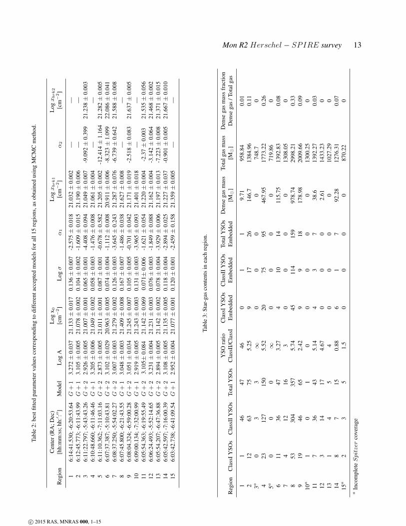
is the one whose reduced χ2 value doesn’t decrease by more than20% while going from simplest to the most complex model. Table1 contains all of the reduced χ2 values. The values for the acceptedmodels are highlighted in bold. The best fitted parameter valueswith their uncertainties as estimated using MCMC for the acceptedmodels are shown in table 2.

Figure 12 shows our adopted sub-division of the Mon R2 col-umn density map into 15 different regions and we have overplot-ted Class I and class II YSOs on the map along with the Spitzer-IRAC mid-IR coverage contour from Gutermuth et al. (2011). Theaccepted model is overlayed on the N-PDF for each region in fig-ure 13. We did not find a region with minimum reduced χ2 for a Gmodel (equation 5) as the most favourable model. We expect a purelognormal behavior for non-star-forming turbulent gas, whereas allof our regions have at least a few YSOs, except region 5 wherewe have incomplete Spitzer sampling. Even regions chosen fortheir low gas density and dearth of YSOs exhibit some small N-PDF excess above the lognormal. The regions that are best fittedby a G + 1 model (equation 6) include all of the well-known em-bedded YSO clusters (e.g. the central Mon R2 cluster is in region8, GGD 17 in region 2, and GGD 12-15 in region 4; Gutermuthet al. 2009) centered on visually obvious gas “hubs” with filamen-tary structures radiating outward (Myers 2009). Finally, the G+ 2model (equation 7) regions visually appear to be aggregates of sev-eral distinct filamentary gas structures with no dominant dense gashubs, as seen in region 6, 7, 9, 11 and 12. Detailed characterizationsof the radial profiles of gas filaments in nearby clouds show a spa-tially resolved maximum in the column density along the spine ofthe filaments (e.g. Arzoumanian et al. 2011). Thus, in the N-PDFsof regions which consist of aggregate of filaments, we see a down-turn of the N-PDF near the maximum density of the most massivefilament. These regions correspond to relatively diffuse and youngYSO distributions, and will be discussed further below.

To understand how the star formation properties depend onthe gas properties, we compare the number of sources to both thepower law exponent and the mass, all of which are tabulated in Ta-ble 3. For studying the variation of the power law index with theYSO count, we have considered the power law index from both

Figure 14. Total number of YSOs vs. first power law index of the best fittedN-PDF model by region. Uncertainties in YSO count follow Poisson statis-tics whereas the power law index uncertainies are obtained from MarkovChain Monte Carlo fits. The numbers associated with the data points referto the region number (cf. figure 12). A steep correlation is seen for the re-gions that are defined by G + 1 models. The dependence is present, butshallower, for the regions defined by G+ 2 models.

G+1 andG+2 models. For the N-PDFs with two power laws, weuse the first index because the second power law index generallyseems to represent a cut-off at some near-maximal N(H2) value,likely set by the peak column density of the densest filament in theaggregate. The total gas mass is calculated by integrating massesover every positive pixel value for each region. Lombardi, Alves &Lada (2015) have called into question the robustness of Herschelderived N(H2) values below AK ∼ 0.1 mag (∼1021 cm−2). Theupper limit to the effect this may have on our masses is given by ahypothetical box of 6.5× 6.5 pc with a mean extinction of 0.1 AK ;this box has a total mass of∼673 M�. This is a substantial fractionof the reported total mass in the regions with low mean N(H2), suchas regions 3 and 5. Finally, YSOs are counted by the data presentedin Gutermuth et al. (2011) for each of the 15 regions; we only in-clude YSOs superimposed on gas column densities in excess ofN(H2) > 1022 cm−2 (e.g. Battisti & Heyer 2014). We note that afew regions (3, 5, 10, 15) are not fully surveyed by Spitzer, howeverthe preponderance of low column density gas in the missed areassuggests that at most a few YSOs would be omitted from thoseregions (Gutermuth et al. 2011).

In previous studies, it has been shown that the exponent ofthe power law component relative to the lognormal component ofan N-PDF correlates with more active star formation (Kainulainenet al. 2009). We find this same correlation within the Mon R2 cloud.In figure 14, we see a correlation between YSO count and the firstpower law index (α1) when these data are separated by the N-PDFmodel type (Pearson coefficient 0.91 and 0.93 for G+ 1 and G+ 2types, respectively). The correlation is steeper in the case of thesingle power law models, while it is shallower for those with twopower laws. Since the single law power laws PDFs have a higherfraction of gas mass at higher column densities, the higher numberof YSOs in these regions may result from a higher star formationrate density and more efficient star formation at these high gas den-sities (Gutermuth et al. 2011).

We also find a clear correlation between YSO mass and thetotal gas mass when we integrate over the N-PDF within the highcolumn density regime. In figure 15, we plot the dense gas mass

c© 2015 RAS, MNRAS 000, 1–15

12 Pokhrel et al.

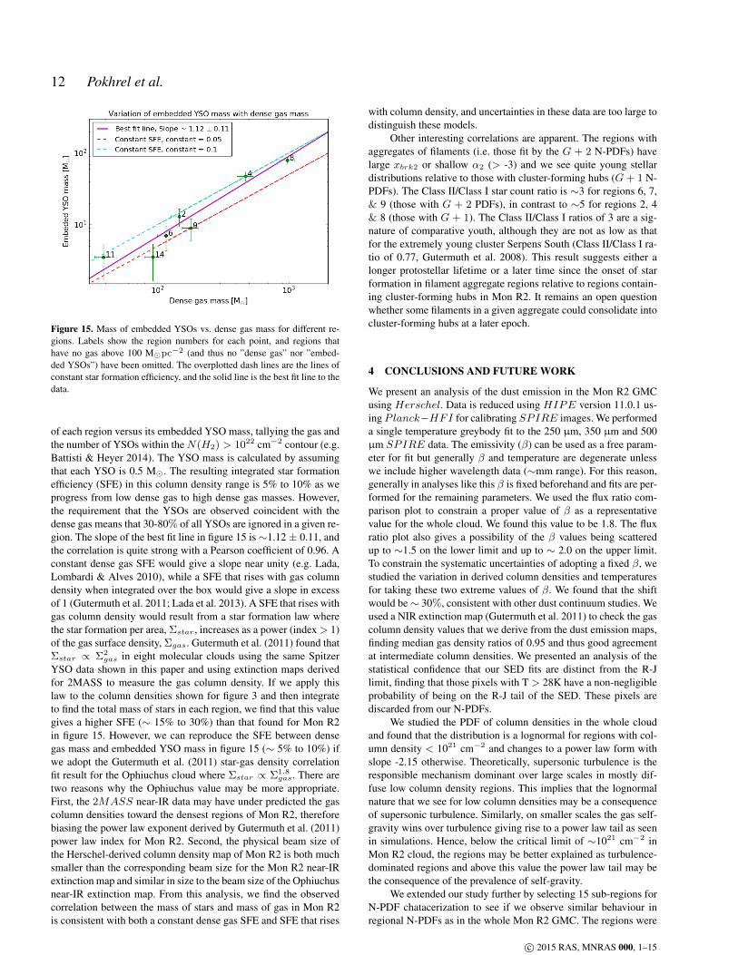
Figure 15. Mass of embedded YSOs vs. dense gas mass for different re-gions. Labels show the region numbers for each point, and regions thathave no gas above 100 M�pc−2 (and thus no ”dense gas” nor ”embed-ded YSOs”) have been omitted. The overplotted dash lines are the lines ofconstant star formation efficiency, and the solid line is the best fit line to thedata.

of each region versus its embedded YSO mass, tallying the gas andthe number of YSOs within theN(H2) > 1022 cm−2 contour (e.g.Battisti & Heyer 2014). The YSO mass is calculated by assumingthat each YSO is 0.5 M�. The resulting integrated star formationefficiency (SFE) in this column density range is 5% to 10% as weprogress from low dense gas to high dense gas masses. However,the requirement that the YSOs are observed coincident with thedense gas means that 30-80% of all YSOs are ignored in a given re-gion. The slope of the best fit line in figure 15 is∼1.12± 0.11, andthe correlation is quite strong with a Pearson coefficient of 0.96. Aconstant dense gas SFE would give a slope near unity (e.g. Lada,Lombardi & Alves 2010), while a SFE that rises with gas columndensity when integrated over the box would give a slope in excessof 1 (Gutermuth et al. 2011; Lada et al. 2013). A SFE that rises withgas column density would result from a star formation law wherethe star formation per area, Σstar , increases as a power (index> 1)of the gas surface density, Σgas. Gutermuth et al. (2011) found thatΣstar ∝ Σ2

gas in eight molecular clouds using the same SpitzerYSO data shown in this paper and using extinction maps derivedfor 2MASS to measure the gas column density. If we apply thislaw to the column densities shown for figure 3 and then integrateto find the total mass of stars in each region, we find that this valuegives a higher SFE (∼ 15% to 30%) than that found for Mon R2in figure 15. However, we can reproduce the SFE between densegas mass and embedded YSO mass in figure 15 (∼ 5% to 10%) ifwe adopt the Gutermuth et al. (2011) star-gas density correlationfit result for the Ophiuchus cloud where Σstar ∝ Σ1.8

gas. There aretwo reasons why the Ophiuchus value may be more appropriate.First, the 2MASS near-IR data may have under predicted the gascolumn densities toward the densest regions of Mon R2, thereforebiasing the power law exponent derived by Gutermuth et al. (2011)power law index for Mon R2. Second, the physical beam size ofthe Herschel-derived column density map of Mon R2 is both muchsmaller than the corresponding beam size for the Mon R2 near-IRextinction map and similar in size to the beam size of the Ophiuchusnear-IR extinction map. From this analysis, we find the observedcorrelation between the mass of stars and mass of gas in Mon R2is consistent with both a constant dense gas SFE and SFE that rises

with column density, and uncertainties in these data are too large todistinguish these models.

Other interesting correlations are apparent. The regions withaggregates of filaments (i.e. those fit by the G + 2 N-PDFs) havelarge xbrk2 or shallow α2 (> -3) and we see quite young stellardistributions relative to those with cluster-forming hubs (G+ 1 N-PDFs). The Class II/Class I star count ratio is ∼3 for regions 6, 7,& 9 (those with G + 2 PDFs), in contrast to ∼5 for regions 2, 4& 8 (those with G + 1). The Class II/Class I ratios of 3 are a sig-nature of comparative youth, although they are not as low as thatfor the extremely young cluster Serpens South (Class II/Class I ra-tio of 0.77, Gutermuth et al. 2008). This result suggests either alonger protostellar lifetime or a later time since the onset of starformation in filament aggregate regions relative to regions contain-ing cluster-forming hubs in Mon R2. It remains an open questionwhether some filaments in a given aggregate could consolidate intocluster-forming hubs at a later epoch.

4 CONCLUSIONS AND FUTURE WORK

We present an analysis of the dust emission in the Mon R2 GMCusing Herschel. Data is reduced using HIPE version 11.0.1 us-ingPlanck−HFI for calibrating SPIRE images. We performeda single temperature greybody fit to the 250 µm, 350 µm and 500µm SPIRE data. The emissivity (β) can be used as a free param-eter for fit but generally β and temperature are degenerate unlesswe include higher wavelength data (∼mm range). For this reason,generally in analyses like this β is fixed beforehand and fits are per-formed for the remaining parameters. We used the flux ratio com-parison plot to constrain a proper value of β as a representativevalue for the whole cloud. We found this value to be 1.8. The fluxratio plot also gives a possibility of the β values being scatteredup to ∼1.5 on the lower limit and up to ∼ 2.0 on the upper limit.To constrain the systematic uncertainties of adopting a fixed β, westudied the variation in derived column densities and temperaturesfor taking these two extreme values of β. We found that the shiftwould be∼ 30%, consistent with other dust continuum studies. Weused a NIR extinction map (Gutermuth et al. 2011) to check the gascolumn density values that we derive from the dust emission maps,finding median gas density ratios of 0.95 and thus good agreementat intermediate column densities. We presented an analysis of thestatistical confidence that our SED fits are distinct from the R-Jlimit, finding that those pixels with T > 28K have a non-negligibleprobability of being on the R-J tail of the SED. These pixels arediscarded from our N-PDFs.

We studied the PDF of column densities in the whole cloudand found that the distribution is a lognormal for regions with col-umn density < 1021 cm−2 and changes to a power law form withslope -2.15 otherwise. Theoretically, supersonic turbulence is theresponsible mechanism dominant over large scales in mostly dif-fuse low column density regions. This implies that the lognormalnature that we see for low column densities may be a consequenceof supersonic turbulence. Similarly, on smaller scales the gas self-gravity wins over turbulence giving rise to a power law tail as seenin simulations. Hence, below the critical limit of ∼1021 cm−2 inMon R2 cloud, the regions may be better explained as turbulence-dominated regions and above this value the power law tail may bethe consequence of the prevalence of self-gravity.

We extended our study further by selecting 15 sub-regions forN-PDF chatacerization to see if we observe similar behaviour inregional N-PDFs as in the whole Mon R2 GMC. The regions were

c© 2015 RAS, MNRAS 000, 1–15

Mon R2 Herschel − SPIRE survey 13Ta

ble

2:be

stfit

ted

para

met

erva

lues

corr

espo

ndin

gto

diff

eren

tacc

epte

dm

odel

sfo

rall

15re

gion

s,as

obta

ined

usin

gM

CM

Cm

etho

d.

Cen

ter(

RA

;Dec

)L

ogx 0

Logxbrk1

Logxbrk2

Reg

ion

[hh:

mm

:ss;

hh:′ :′′

]M

odel

Log

A[c

m−2]

Logσ

α1

[cm−2]

α2

[cm−2]

16:

14:4

1.53

0;-6

:20:

53.6

4G

+1

3.27

2±

0.03

721

.133±

0.01

70.

136±

0.00

7-2

.575±

0.01

821

.032±

0.00

2—

—2

6:12

:45.

773;

-6:1

1:43

.99

G+

13.

105±

0.00

521

.078±

0.00

20.

104±

0.00

2-1

.609±

0.01

521

.190±

0.00

6—

—3

6:11

:22.

797;

-5:4

3:43

.26

G+

22.

926±

0.00

521

.007±

0.00

10.

065±

0.00

1-4

.408±

0.09

421

.049±

0.00

7-9

.092±

0.39

921

.238±

0.00

34

6:10

:48.

660;

-6:1

1:46

.46

G+

13.

205±

0.00

621

.049±

0.00

20.

058±

0.00

3-1

.476±

0.00

821

.061±

0.00

4—

—5

6:11

:10.

362;

-7:1

1:03

.16

G+

22.

873±

0.00

521

.011±

0.00

10.

087±

0.00

1-0

.678±

0.58

221

.205±

0.00

2-1

2.41

4±

1.16

421

.282±

0.00

56

6:07

:37.

387;

-5:1

0:43

.81

G+

23.

102±

0.02

920

.963±

0.00

50.

074±

0.00

4-1

.112±

0.00

820

.911±

0.00

6-8

.323±

1.09

922

.086±

0.04

17

6:08

:37.

250;

-5:5

4:02

.27

G+

23.

007±

0.00

321

.279±

0.00

20.

126±

0.00

3-3

.645±

0.24

321

.287±

0.07

6-6

.739±

0.64

221

.588±

0.00

88

6:07

:45.

800;

-6:2

1:43

.55

G+

13.

048±

0.00

321

.409±

0.00

80.

167±

0.00

7-1

.486±

0.03

821

.627±

0.00

8—

—9

6:08

:04.

324;

-6:5

9:00

.28

G+

23.

051±

0.03

421

.245±

0.00

70.

105±

0.00

5-0

.701±

0.04

221

.171±

0.01

9-2

.518±

0.08

321

.637±

0.00

510

6:09

:00.

134;

-7:3

2:00

.99

G+

12.

919±

0.00

521

.243±

0.00

30.

131±

0.00

3-3

.965±

0.09

321

.401±

0.01

8—

—11

6:05

:54.

363;

-6:1

9:55

.49

G+

23.

105±

0.08

421

.142±

0.06

90.

071±

0.00

6-1

.621±

0.05

421

.220±

0.00

4-2

.37±

0.00

321

.535±

0.05

612

6:06

:24.

493;

-5:5

2:14

.65

G+

23.

231±

0.00

421

.231±

0.00

30.

076±

0.00

3-1

.849±

0.08

821

.162±

0.00

4-3

.142±

0.06

421

.468±

0.00

213

6:05

:54.

207;

-6:4

7:36

.88

G+

22.

894±

0.00

521

.142±

0.00

20.

078±

0.00

4-3

.929±

0.00

621

.197±

0.01

3-7

.223±

0.00

821

.371±

0.01

514

6:05

:42.

597;

-7:1

6:00

.39

G+

23.

108±

0.00

521

.135±

0.00

50.

118±

0.00

4-2

.894±

0.02

521

.227±

0.03

7-0

.901±

0.00

521

.667±

0.01

015

6:03

:42.

738;

-6:4

1:09

.54

G+

12.

952±

0.00

421

.077±

0.00

10.

120±

0.00

1-2

.459±

0.15

821

.359±

0.00

5—

—

Tabl

e3:

Star

-gas

cont

ents

inea

chre

gion

.

YSO

ratio

Cla

ssIY

SOs

Cla

ssII

YSO

sTo

talY

SOs

Den

sega

sm

ass

Tota

lgas

mas

sD

ense

gas

mas

sfr

actio

nR

egio

nC

lass

IYSO

sC

lass

IIY

SOs

Tota

lYSO

sC

lass

II/C

lass

IE

mbe

dded

Em

bedd

edE

mbe

dded

[M�

][M�

]D

ense

gas

/Tot

alga

s

11

4647

460

11

9.71

958.

840.

012

1263

755.

259

1726

146.

713

84.9

60.

113a

03

3∞

00

00

748.

70

423

127

150

5.52

2075

9546

7.95

1773

.22

0.26

5a0

00

∞0

00

071

9.86

06

1136

473.

274

1014

115.

7513

92.8

30.

087

412

163

00

00

1308

.05

08

5330

435

75.

7445

114

159

978.

7429

98.2

10.

339

1946

652.

429

918

178.

9820

09.6

60.

0910a

10

10

00

00

1300

.25

011

736

435.

144

37

38.6

1392

.27

0.03

123

1417

4.67

00

02.

6114

33.2

30

131

45

40

00

010

27.2

90

148

715

0.88

61

792

.28

1276

.31

0.07

15a

23

51.

50

00

087

0.22

0

aIn

com

plet

eSpitzer

cove

rage

c© 2015 RAS, MNRAS 000, 1–15

14 Pokhrel et al.

fixed in size and selected to span a range of YSO densitiy envi-ronments. For all regions that contain dense YSO cluster cores, theN-PDF is a combination of a lognormal and one power law func-tion. We do not see the power law excess in high column densityregion of the Mon R2 cluster core, as reported by Schneider et al.(2015a). The regions with moderate numbers of YSOs and densefilamentary structures are better explained by a lognormal with twopower laws.

We studied how the power law index of N-PDFs, oftenclaimed to be a defining factor of star formation, varies with theYSO count in several regions of Mon R2. For the regions definedby a single power law, we found that the correlation is steeper thanfor the regions defined by two power laws. In the latter case, theabsence of high column density gas signifies lower star formationefficiency and thus less YSOs. While doing the regional analysis,we estimated the dense gas mass in each region and did a qualita-tive study of their relation with the YSO count that are embeddedin the dense gas. We see a clear correlation of the dense gas masswith the embedded YSO count, but we lacked sufficient statisticalconstraint to differentiate between models that suggest the SFE isconstant or rising with higher dense gas mass.

The emergence of the single power law in N-PDFs is often re-lated with high star formation in those regions, but the presence ofthe second power law is still not fully understood. However, look-ing at the gas geometry in those regions, it seems to be related tothe presence of dense filament aggregates. This leaves us with fur-ther open questions. Are these filament aggregates, which are rep-resented in N-PDF by a shallow power law with steep cut-off atintermediate density, distinctly different structures from seeminglymore monolithic clustered star forming sites that exhibit singlepower law N-PDFs? Do the filament aggregates coalesce into themore monolithic cluster-forming sites, thereby evolving to reach ageometry where higher gas densities are achieved and stars can beformed considerably more efficiently? A more detailed work thatincorporates other nearby molecular clouds is required to addressthese questions and is beyond the scope of this paper.

This work is based on observations made with Herschel,a European Space Agency cornerstone mission with significantparticipation by NASA. Support for this work was provided byNASA through an award issued by JPL/Caltech (contract number1489384). S. J. Wolk was supported by NASA contract NAS8-03060. We are thankful to Stella Offner, Mark Heyer, Grant Wilsonand Ronald Snell from the University of Massachusetts (UMASS),Amherst for helpful conversations, suggestions, and feedback. Wealso thank Amy Stutz of the Max-Planck Institute for Astron-omy, Germany for important suggestions on the paper. We alsothank Bernhard Schulz and David Shupe from NASA HerschelScience Center for helping us with data reduction. We are grate-ful to Manikarajamuthaly Sri Saravana and Joan Chamberlin forhelping us with technical aspects. Finally, we would like to thankthe anonymous referee for valuable comments and suggestions.SPIRE has been developed by a consortium of institutes ledby Cardiff Univ. (UK) and including Univ. Lethbridge (Canada);NAOC (China); CEA, LAM (France); IFSI, Univ. Padua (Italy);IAC (Spain); Stockholm Observatory (Sweden); Imperial Col-lege London, RAL, UCL-MSSL, UKATC, Univ. Sussex (UK);Caltech, JPL, NHSC, Univ. Colorado (USA). This developmenthas been supported by national funding agencies: CSA (Canada);NAOC (China); CEA, CNES, CNRS (France); ASI (Italy); MCINN(Spain); SNSB (Sweden); STFC (UK); and NASA (USA). PACShas been developed by a consortium of institutes led by MPE (Ger-many) and including UVIE (Austria); KUL, CSL, IMEC (Bel-

gium); CEA, OAMP (France); MPIA (Germany); IFSI, OAP/AOT,OAA/CAISMI, LENS, SISSA (Italy); IAC (Spain). This develop-ment has been supported by the funding agencies BMVIT (Aus-tria), ESA-PRODEX (Belgium), CEA/CNES (France), DLR (Ger-many), ASI (Italy), and CICT/MCT (Spain).

REFERENCES

Andre P. et al., 2010, A&A, 518, L102Aniano G., Draine B. T., Gordon K. D., Sandstrom K., 2011,

PASP, 123, 1218Arzoumanian D. et al., 2011, A&A, 529, L6Battisti A. J., Heyer M. H., 2014, ApJ, 780, 173Bernard J.-P. et al., 2010, A&A, 518, L88Bohlin R. C., Savage B. D., Drake J. F., 1978, ApJ, 224, 132Brunt C. M., Federrath C., Price D. J., 2010, MNRAS, 405, L56Carpenter J. M., 2000, AJ, 120, 3139Draine B. T., 1978, in Bulletin of the American Astronomical So-

ciety, Vol. 10, Bulletin of the American Astronomical Society, p.463

Federrath C., Klessen R. S., Schmidt W., 2008, ApJ, 688, L79Goodman A. A., Pineda J. E., Schnee S. L., 2009, ApJ, 692, 91Griffin M. J. et al., 2010, A&A, 518, L3Gutermuth R. A. et al., 2008, ApJ, 673, L151Gutermuth R. A., Megeath S. T., Myers P. C., Allen L. E., Pipher

J. L., Fazio G. G., 2009, ApJS, 184, 18Gutermuth R. A., Megeath S. T., Pipher J. L., Williams J. P., Allen

L. E., Myers P. C., Raines S. N., 2005, ApJ, 632, 397Gutermuth R. A., Pipher J. L., Megeath S. T., Myers P. C., Allen

L. E., Allen T. S., 2011, ApJ, 739, 84Herbst W., Racine R., 1976, AJ, 81, 840Hildebrand R. H., 1983, QJRAS, 24, 267Hill T. et al., 2011, A&A, 533, A94Hodapp K. W., 2007, AJ, 134, 2020Johnson H. L., 1963, Photometric Systems, the University of

Chicago Press, p. 204Kainulainen J., Beuther H., Henning T., Plume R., 2009, A&A,

508, L35Klessen R. S., 2000, ApJ, 535, 869Klessen R. S., Heitsch F., Mac Low M.-M., 2000, ApJ, 535, 887Kritsuk A. G., Norman M. L., Wagner R., 2011, ApJ, 727, L20Kutner M. L., Tucker K. D., 1975, ApJ, 199, 79Lada C. J., Lombardi M., Alves J. F., 2010, ApJ, 724, 687Lada C. J., Lombardi M., Roman-Zuniga C., Forbrich J., Alves

J. F., 2013, ApJ, 778, 133Landsman W. B., 1993, in Astronomical Society of the Pacific

Conference Series, Vol. 52, Astronomical Data Analysis Soft-ware and Systems II, Hanisch R. J., Brissenden R. J. V., BarnesJ., eds., p. 246

Lee E. J., Chang P., Murray N., 2014, ArXiv e-printsLombardi M., Alves J., Lada C. J., 2015, A&A, 576, L1Lombardi M., Lada C. J., Alves J., 2008, A&A, 480, 785Loren R. B., Peters W. L., Vanden Bout P. A., 1974, ApJ, 194,

L103Maddalena R. J., Morris M., Moscowitz J., Thaddeus P., 1986,

ApJ, 303, 375Mathis J. S., Rumpl W., Nordsieck K. H., 1977, ApJ, 217, 425McKee C. F., Ostriker E. C., 2007, ARA&A, 45, 565Miesch M. S., Scalo J., Bally J., 1999, ApJ, 524, 895Molina F. Z., Glover S. C. O., Federrath C., Klessen R. S., 2012,

MNRAS, 423, 2680

c© 2015 RAS, MNRAS 000, 1–15

Mon R2 Herschel − SPIRE survey 15

Myers P. C., 2009, ApJ, 700, 1609Ossenkopf V., Henning T., 1994, A&A, 291, 943Ott S., 2010, in Astronomical Society of the Pacific Conference

Series, Vol. 434, Astronomical Data Analysis Software and Sys-tems XIX, Mizumoto Y., Morita K.-I., Ohishi M., eds., p. 139

Padoan P., Federrath C., Chabrier G., Evans, II N. J., JohnstoneD., Jørgensen J. K., McKee C. F., Nordlund A., 2014, Protostarsand Planets VI, 77

Padoan P., Nordlund A., Jones B. J. T., 1997, MNRAS, 288, 145Patil A., Huard D., Fonnesbeck C., 2010, Journal of Statistical

Software, 35, 1Pilbratt G. L. et al., 2010, A&A, 518, L1Planck HFI Core Team et al., 2011, A&A, 536, A4Poglitsch A. et al., 2010, A&A, 518, L2Predehl P., Schmitt J. H. M. M., 1995, A&A, 293, 889Racine R., 1968, AJ, 73, 233Sadavoy S. I. et al., 2012, A&A, 540, A10Sadavoy S. I. et al., 2013, ApJ, 767, 126Schnee S. L., Ridge N. A., Goodman A. A., Li J. G., 2005, ApJ,

634, 442Schneider N. et al., 2015a, ArXiv e-printsSchneider N. et al., 2015b, A&A, 575, A79Seares F. H., Hubble E. P., 1920, ApJ, 52, 8Stutz A. M., Kainulainen J., 2015, A&A, 577, L6Truelove J. K., Klein R. I., McKee C. F., Holliman, II J. H., Howell

L. H., Greenough J. A., 1997, ApJ, 489, L179van Dyk D. A., 2003, Hierarchical models, data augmentation,

and Markov chain Monte Carlo, Springer, pp. 41–56Wood D. O. S., Myers P. C., Daugherty D. A., 1994, ApJS, 95,

457Xie T., 1992, PhD thesis, Univ. of Massachusetts, Amherst

This paper has been typeset from a TEX/ LATEX file prepared by theauthor.

c© 2015 RAS, MNRAS 000, 1–15