appendix f.1 hydrologic and water quality modeling water resources control board california...
TRANSCRIPT

Appendix F.1 Hydrologic and Water Quality Modeling

Evaluation of San Joaquin River Flow and Southern Delta Water Quality Objectives and Implementation
F.1-i September 2016
ICF 00427.11
Appendix F.1 Hydrologic and Water Quality Modeling
Appendix F.1 Hydrologic and Water Quality Modeling ......................................................................F.1-i
F.1.1 Introduction .................................................................................................................. F.1-1
F.1.2 Water Supply Effects Modeling—Methods .................................................................. F.1-2
F.1.2.1 U.S. Bureau of Reclamation CALSIM II SJR Module ................................................ F.1-4
F.1.2.2 Development of the WSE Model Baseline and Alternative Assumptions .............. F.1-6
F.1.2.3 Calculation of Flow Targets .................................................................................. F.1-13
F.1.2.4 Calculation of Monthly Surface Water Demand .................................................. F.1-19
F.1.2.5 Calculation of Available Water for Diversion ....................................................... F.1-30
F.1.2.6 Calculation of Surface Water Diversion Allocation .............................................. F.1-38
F.1.2.7 Calculation of River and Reservoir Water Balance ............................................... F.1-40
F.1.3 Water Supply Effects Modeling—Results ................................................................... F.1-57
F.1.3.1 Summary of Water Supply Effects Model Results ................................................ F.1-57
F.1.3.2 Characterization of Baseline Conditions .............................................................. F.1-80
F.1.3.3 20 Percent Unimpaired Flow (LSJR Alternative 2) .............................................. F.1-105
F.1.3.4 40 Percent Unimpaired Flow (LSJR Alternative 3) .............................................. F.1-118
F.1.3.5 60 Percent Unimpaired Flow (LSJR Alternative 4) .............................................. F.1-130
F.1.4 Comparison of the Cumulative Distributions of Monthly Flows .............................. F.1-143
F.1.4.1 Merced River Flows ............................................................................................ F.1-143
F.1.4.2 Tuolumne River Flows ........................................................................................ F.1-151
F.1.4.3 Stanislaus River Flows ........................................................................................ F.1-159
F.1.4.4 SJR at Vernalis Flows .......................................................................................... F.1-167
F.1.5 Salinity Modeling ....................................................................................................... F.1-175
F.1.5.1 Salinity Modeling Methods ................................................................................ F.1-175
F.1.5.2 Salinity Modeling Results ................................................................................... F.1-178
F.1.6 Temperature Modeling ............................................................................................. F.1-190
F.1.6.1 Temperature Model Methods ............................................................................ F.1-191
F.1.6.2 Temperature Model Results ............................................................................... F.1-200
F.1.7 Potential Changes in Delta Exports and Outflow ...................................................... F.1-291
F.1.7.1 Current Operational Summary ........................................................................... F.1-291
F.1.7.2 Methods to Estimate Changes in Delta Exports and Outflow ............................ F.1-292
F.1.7.3 Changes in Delta Exports and Outflow ............................................................... F.1-297
F.1.8 References Cited ....................................................................................................... F.1-310

State Water Resources Control Board California Environmental Protection Agency
Appendix F.1 Hydrologic and Water Quality Modeling
Evaluation of San Joaquin River Flow and Southern Delta Water Quality Objectives and Implementation
F.1-ii September 2016
ICF 00427.11
Tables
Table F.1.1-1. Introduction: Percent Unimpaired Flows by LSJR Alternative ................................... F.1-2
Table F.1.2-1. Stanislaus River Combined CVP Contractor (Stockton East Water District
[SEWD] and Central San Joaquin Water Conservation District [CSJWCD])
Diversion Delivery Curves Based on New Melones Index Used in the WSE
Model ......................................................................................................................... F.1-5
Table F.1.2-2. DWR DRR CALSIM II, USBR CALSIM II, SWRCB CALSIM II, and WSE Baseline
Model Assumptions ................................................................................................... F.1-8
Table F.1.2-3. WSE Modeling Assumptions .................................................................................... F.1-10
Table F.1.2-4. Minimum Monthly Flow Requirements at Goodwin Dam on the Stanislaus
River per NMFS BO Table 2E .................................................................................... F.1-14
Table F.1.2-5. Minimum Monthly Flow Requirements at La Grange Dam on the Tuolumne
River per 1995 FERC Settlement Agreement ........................................................... F.1-15
Table F.1.2-6. Minimum Monthly Flow Requirements and Modeled Flow Requirement at
Shaffer Bridge on the Merced River per FERC 2179 License, Article 40 and 41 ...... F.1-16
Table F.1.2-7. Monthly Cowell Agreement Diversions on the Merced River between Crocker-
Huffman Dam and Shaffer Bridge ............................................................................ F.1-16
Table F.1.2-8. D-1641 Minimum Monthly Flow Requirements and Maximum Salinity
Concentration in the SJR at Airport Way Bridge Near Vernalis ............................... F.1-18
Table F.1.2-9. VAMP Minimum Pulse Flow Requirements in the SJR at Airport Way Bridge
near Vernalis ............................................................................................................ F.1-19
Table F.1.2-10. Division of VAMP Additional Flow per Tributary According to the SJR
Agreement ............................................................................................................... F.1-19
Table F.1.2-11. Calculation of Deep Percolation Factors and Distribution Loss Factors .................. F.1-21
Table F.1.2-12. Other Annual Demands for Each Irrigation District ................................................. F.1-23
Table F.1.2-13. Annual Minimum Groundwater Pumping Estimates for Each Irrigation District .... F.1-24
Table F.1.2-14. Sample of Irrigation District Diversion Data Reported in AWMPs .......................... F.1-25
Table F.1.2-15. Adjustment Factors Applied to CUAW Demands .................................................... F.1-26
Table F.1.2-16. Annual Irrigation Year (Mar-Feb) Diversions from the Stanislaus River by
OID/SSJID, as Represented by USGS Observed, CALSIM, Stanislaus Operations
Model, WSE-CALSIM Baseline, WSE-CEQA Baseline, and AWMP Data ................... F.1-26
Table F.1.2-17. Annual Irrigation Year (Mar-Feb) Diversions from the Tuolumne River by
MID/TID, as Represented by USGS Observed, SWRCB-CALSIM, Tuolumne

State Water Resources Control Board California Environmental Protection Agency
Appendix F.1 Hydrologic and Water Quality Modeling
Evaluation of San Joaquin River Flow and Southern Delta Water Quality Objectives and Implementation
F.1-iii September 2016
ICF 00427.11
Operations Model, WSE-CALSIM Baseline, WSE-CEQA Baseline, and AWMP
Data ......................................................................................................................... F.1-28
Table F.1.2-18. Annual Irrigation Year (Mar-Feb) Diversions from the Merced River by Merced
ID, as Represented by Observed, CALSIM, Merced Operations Model, WSE
w/CALSIM parameters, WSE-CEQA Baseline, and AWMP Data .............................. F.1-29
Table F.1.2-19. CVP Contractor Monthly Diversion Schedule .......................................................... F.1-30
Table F.1.2-20. Baseline End-of-September Storage Guidelines, Maximum Draw from Storage,
and Minimum Diversion Variables for the Eastside Tributaries .............................. F.1-34
Table F.1.2-21a. Area/Volume Relationship for New Melones Reservoir for Calculating
Evaporation ............................................................................................................. F.1-34
Table F.1.2-21b. Area/Volume Relationship for New Don Pedro Reservoir for Calculating
Evaporation ............................................................................................................. F.1-34
Table F.1.2-21c. Area/Volume Relationship for New Exchequer Reservoir for Calculating
Evaporation ............................................................................................................. F.1-35
Table F.1.2-22. Annual Average Evaporation for New Melones, New Don Pedro, and New
Exchequer Reservoirs for Baseline and LSJR Alternatives ....................................... F.1-35
Table F.1.2-23a. Minimum Diversion, Minimum September Carryover Guideline, Maximum
Draw from Storage, and Flow Shifting for the Stanislaus River............................... F.1-36
Table F.1.2-23b. Minimum Diversion, Minimum September Carryover Guideline, Maximum
Draw from Storage, and Adaptive Implementation for the Tuolumne River .......... F.1-37
Table F.1.2-23c. Minimum Diversion, Minimum September Carryover Guideline, Maximum
Draw from Storage, and Flow Shifting for the Merced River .................................. F.1-38
Table F.1.2-24. CALSIM End-of-Month Flood Control Storage Limitations Applied to New
Melones Reservoir, New Don Pedro Reservoir, and Lake McClure in the WSE
Model ....................................................................................................................... F.1-41
Table F.1.2-25. Instream Flow Targets July–November that Determine Necessary Volume of
Flow Shifting from the February–June Period for the (a) Stanislaus, (b)
Tuolumne, and (c) Merced Rivers for Each Water Year Type ................................. F.1-44
Table F.1.2-26. Average Quantity of Flow Shifted to Fall for the Stanislaus, Tuolumne, and
Merced Rivers for Each Water Year Type ................................................................ F.1-45
Table F.1.3-1a. Average Carryover Storage within the Three Major Reservoirs over the 82-
Year Modeling Period (TAF) ..................................................................................... F.1-58
Table F.1.3-1b. Average Carryover Storage during Critically Dry Years within the Three Major
Reservoirs over the 82-Year Modeling Period (TAF) ............................................... F.1-58
State Water Resources Control Board California Environmental Protection Agency
Appendix F.1 Hydrologic and Water Quality Modeling
Evaluation of San Joaquin River Flow and Southern Delta Water Quality Objectives and Implementation
F.1-iv September 2016
ICF 00427.11
Table F.1.3-2a. Average Baseline Streamflow and Differences from Baseline Conditions on the
Eastside Tributaries and near Vernalis .................................................................... F.1-62
Table F.1.3-2b. Mean Annual February–June Instream Flow in the Plan Area by Water Year
Type ......................................................................................................................... F.1-64
Table F.1.3-3. Average Annual Baseline Water Supply and Difference from Baseline
Conditions on the Eastside Tributaries and Plan Area Totals over the 82-year
Modeling Period ...................................................................................................... F.1-69
Table F.1.3-4a. Annual Water Supply Diversions for Baseline Conditions and Percent of
Unimpaired Flow on the Stanislaus ......................................................................... F.1-70
Table F.1.3-4b. Annual Water Supply Diversions for Baseline Conditions and Percent of
Unimpaired Flow on the Tuolumne ......................................................................... F.1-70
Table F.1.3-4c. Annual Water Supply Diversions for Baseline Conditions and Percent of
Unimpaired Flow on the Merced ............................................................................ F.1-71
Table F.1.3-4d. Mean Annual Diversions Under 40 Percent Unimpaired Flow Proposal by
Water Year Type ...................................................................................................... F.1-72
Table F.1.3-5a. Baseline Monthly Cumulative Distributions of SJR above the Merced Flow (cfs)
for 1922–2003 ......................................................................................................... F.1-81
Table F.1.3-5b. Simulated Baseline Monthly Cumulative Distributions of Lake McClure Storage
for 1922–2003 ......................................................................................................... F.1-83
Table F.1.3-5c. Simulated Baseline Monthly Cumulative Distributions of Lake McClure Water
Surface Elevations (feet MSL) for 1922–2003 ......................................................... F.1-84
Table F.1.3-5d. Baseline Monthly Cumulative Distributions of Target Flows (cfs) for the
Merced River at Stevinson for 1922–2003 .............................................................. F.1-86
Table F.1.3-5e. Baseline Monthly Cumulative Distributions of Merced River at Stevinson Flow
(cfs) for 1922–2003 .................................................................................................. F.1-87
Table F.1.3-5f. CALSIM-Simulated Baseline Monthly Cumulative Distributions of New Don
Pedro Reservoir Inflow (TAF) for 1922–2003 .......................................................... F.1-90
Table F.1.3-5g. CALSIM-Simulated Baseline Monthly Cumulative Distributions of CCSF
Upstream Diversions and Reservoir Operations (TAF) for 1922–2003 ................... F.1-90
Table F.1.3-5h. Baseline Monthly Cumulative Distributions of New Don Pedro Reservoir
Storage (TAF) for 1922–2003 ................................................................................... F.1-91
Table F.1.3-5i. Baseline Monthly Cumulative Distributions of New Don Pedro Water Surface
Elevations (feet MSL) for 1922–2003 ...................................................................... F.1-92
Table F.1.3-5j. Baseline Monthly Cumulative Distributions of Target Flows (cfs) for the
Tuolumne River at Modesto for 1922–2003 ........................................................... F.1-94
State Water Resources Control Board California Environmental Protection Agency
Appendix F.1 Hydrologic and Water Quality Modeling
Evaluation of San Joaquin River Flow and Southern Delta Water Quality Objectives and Implementation
F.1-v September 2016
ICF 00427.11
Table F.1.3-5k. Baseline Monthly Cumulative Distributions of Tuolumne River at Modesto
Flow (cfs) for 1922–2003 ......................................................................................... F.1-95
Table F.1.3-5l. Baseline Monthly Cumulative Distributions of New Melones Storage (TAF) for
1922–2003 ............................................................................................................... F.1-98
Table F.1.3-5m. Baseline Monthly Cumulative Distributions of New Melones Water Surface
Elevations (feet MSL) for 1922–2003 ...................................................................... F.1-99
Table F.1.3-5n. Baseline Monthly Cumulative Distributions of Target Flows (cfs) for the
Stanislaus River at Ripon for 1922–2003 ............................................................... F.1-101
Table F.1.3-5o. Baseline Monthly Cumulative Distributions of Stanislaus River at Ripon Flow
(cfs) for 1922–2003 ................................................................................................ F.1-102
Table F.1.3-5p. Baseline Monthly Cumulative Distributions of SJR at Vernalis Flow (cfs) for
1922–2003 ............................................................................................................. F.1-104
Table F.1.3-6a. WSE Results for Lake McClure Storage (TAF) for 20% Unimpaired Flow (LSJR
Alternative 2) ......................................................................................................... F.1-106
Table F.1.3-6b. WSE Results for Lake McClure Water Surface Elevations (feet MSL) for 20%
Unimpaired Flow (20% Unimpaired Flow) ............................................................ F.1-106
Table F.1.3-6c. Merced River Target Flows (cfs) for 20% Unimpaired Flow (LSJR Alternative 2) .. F.1-107
Table F.1.3-6d. Merced River Flows at Stevinson (cfs) for 20% Unimpaired Flow (LSJR
Alternative 2) ......................................................................................................... F.1-108
Table F.1.3-6e. WSE Results for New Don Pedro Storage (TAF) for 20% Unimpaired Flow (LSJR
Alternative 2) ......................................................................................................... F.1-109
Table F.1.3-6f. WSE Results for New Don Pedro Water Surface Elevations (feet MSL) for 20%
Unimpaired Flow (LSJR Alternative 2) ................................................................... F.1-110
Table F.1.3-6g. Tuolumne River Target Flows (cfs) for 20% Unimpaired Flow (LSJR Alternative
2) ............................................................................................................................ F.1-111
Table F.1.3-6h. Tuolumne River Flows at Modesto (cfs) for 20% Unimpaired Flow (LSJR
Alternative 2) ......................................................................................................... F.1-112
Table F.1.3-6i. WSE Results for New Melones Storage (TAF) for 20% Unimpaired Flow (LSJR
Alternative 2) ......................................................................................................... F.1-113
Table F.1.3-6j. WSE Results for New Melones Water Surface Elevations (feet MSL) for 20%
Unimpaired Flow (LSJR Alternative 2) ................................................................... F.1-113
Table F.1.3-6k. Stanislaus River Target Flows (cfs) for 20% Unimpaired Flow (LSJR Alternative
2) ............................................................................................................................ F.1-114

State Water Resources Control Board California Environmental Protection Agency
Appendix F.1 Hydrologic and Water Quality Modeling
Evaluation of San Joaquin River Flow and Southern Delta Water Quality Objectives and Implementation
F.1-vi September 2016
ICF 00427.11
Table F.1.3-6l. Stanislaus River Flows at Ripon (cfs) for 20% Unimpaired Flow (LSJR
Alternative 2) ......................................................................................................... F.1-115
Table F.1.3-6m. SJR Flows at Vernalis (cfs) for 20% Unimpaired Flow (LSJR Alternative 2) ............ F.1-117
Table F.1.3-7a. WSE Results for Lake McClure Storage (TAF) for 40% Unimpaired Flow (LSJR
Alternative 3) ......................................................................................................... F.1-118
Table F.1.3-7b. WSE Results for Lake McClure Water Surface Elevation (feet MSL) for 40%
Unimpaired Flow (LSJR Alternative 3) ................................................................... F.1-119
Table F.1.3-7c. Merced River Target Flows (cfs) for 40% Unimpaired Flow (LSJR Alternative 3) .. F.1-119
Table F.1.3-7d. Merced River Flows at Stevinson (cfs) for 40% Unimpaired Flow (LSJR
Alternative 3) ......................................................................................................... F.1-121
Table F.1.3-7e. WSE Results for New Don Pedro Reservoir Storage (TAF) for 40% Unimpaired
Flow (LSJR Alternative 3) ....................................................................................... F.1-122
Table F.1.3-7f. WSE Results for New Don Pedro Reservoir Water Surface Elevation (feet MSL)
for 40% Unimpaired Flow (LSJR Alternative 3) ...................................................... F.1-122
Table F.1.3-7g. Tuolumne River Target Flows (cfs) for 40% Unimpaired Flow (LSJR Alternative
3) ............................................................................................................................ F.1-123
Table F.1.3-7h. Tuolumne River Flows at Modesto (cfs) for 40% Unimpaired Flow (LSJR
Alternative 3) ......................................................................................................... F.1-124
Table F.1.3-7i. WSE Results for New Melones Reservoir Storage (TAF) for 40% Unimpaired
Flow (LSJR Alternative 3) ....................................................................................... F.1-125
Table F.1.3-7j. WSE Results for New Melones Reservoir Water Surface Elevation (feet MSL)
for 40% Unimpaired Flow (LSJR Alternative 3) ...................................................... F.1-125
Table F.1.3-7k. Stanislaus River Target Flows (cfs) for 40% Unimpaired Flow (LSJR Alternative
3) ............................................................................................................................ F.1-126
Table F.1.3-7l. Stanislaus River Flows at Ripon (cfs) for 40% Unimpaired Flow (LSJR
Alternative 3) ......................................................................................................... F.1-127
Table F.1.3-7m. SJR Flows at Vernalis (cfs) for 40% Unimpaired Flow (LSJR Alternative 3) ............ F.1-129
Table F.1.3-8a. WSE Results for Lake McClure Storage (TAF) for 60% Unimpaired Flow (LSJR
Alternative 4) ......................................................................................................... F.1-130
Table F.1.3-8b. WSE Results for Lake McClure Water Surface Elevations (feet MSL) for 60%
Unimpaired Flow (LSJR Alternative 4) ................................................................... F.1-131
Table F.1.3-8c. Merced River Target Flows (cfs) for 60% Unimpaired Flow (LSJR Alternative 4) .. F.1-131
Table F.1.3-8d. Merced River Flows at Stevinson (cfs) for 60% Unimpaired Flow (LSJR
Alternative 4) ......................................................................................................... F.1-133

State Water Resources Control Board California Environmental Protection Agency
Appendix F.1 Hydrologic and Water Quality Modeling
Evaluation of San Joaquin River Flow and Southern Delta Water Quality Objectives and Implementation
F.1-vii September 2016
ICF 00427.11
Table F.1.3-8e. WSE Results for New Don Pedro Reservoir Storage (TAF) for 60% Unimpaired
Flow (LSJR Alternative 4) ....................................................................................... F.1-134
Table F.1.3-8f. WSE Results for New Don Pedro Reservoir Water Surface Elevations (feet
MSL) for 60% Unimpaired Flow (LSJR Alternative 4) ............................................. F.1-135
Table F.1.3-8g. Tuolumne River Target Flows (cfs) for 60% Unimpaired Flow (LSJR Alternative
4) ............................................................................................................................ F.1-135
Table F.1.3-8h. Tuolumne River Flows at Modesto (cfs) for 60% Unimpaired Flow (LSJR
Alternative 4) ......................................................................................................... F.1-137
Table F.1.3-8i. WSE Results for New Melones Reservoir Storage (TAF) for 60% Unimpaired
Flow (LSJR Alternative 4) ....................................................................................... F.1-138
Table F.1.3-8j. WSE Results for New Melones Reservoir Water Surface Elevations (feet MSL)
for 60% Unimpaired Flow (LSJR Alternative 4) ...................................................... F.1-138
Table F.1.3-8k. Stanislaus River Target Flows (cfs) for 60% Unimpaired Flow (LSJR Alternative
4) ............................................................................................................................ F.1-139
Table F.1.3-8l. Stanislaus River Flows at Ripon (cfs) for 60% Unimpaired Flow (LSJR
Alternative 4) ......................................................................................................... F.1-140
Table F.1.3-8m. SJR Flows at Vernalis (cfs) for 60% Unimpaired Flow (LSJR Alternative 4) ............ F.1-142
Table F.1.4-1. Cumulative Distributions of February–June River Flow Volumes (TAF) in the
Merced River at Stevinson for Baseline Conditions and the Percent
Unimpaired Flow Simulations (20%–60%)............................................................. F.1-144
Table F.1.4-2. Cumulative Distributions of February–June River Flow Volumes (TAF) in the
Tuolumne River at Modesto for Baseline Conditions and the Unimpaired Flow
Simulations (20%–60%) ......................................................................................... F.1-152
Table F.1.4-3. Cumulative Distributions of February–June River Flow Volumes (TAF) in the
Stanislaus River at Ripon for Baseline Conditions and the Percent Unimpaired
Flow Simulations (20%–60%) ................................................................................. F.1-160
Table F.1.4-4. Cumulative Distributions of February–June River Flow Volumes (TAF) of SJR at
Vernalis for Baseline Conditions and the Unimpaired Flow Simulations (20%–
60%) ....................................................................................................................... F.1-168
Table F.1.5-1a. CALSIM-Simulated Baseline Monthly Cumulative Distributions of SJR above
the Merced EC (µS/cm) 1922–2003 ...................................................................... F.1-180
Table F.1.5-1b. Baseline Monthly Cumulative Distributions of SJR at Vernalis EC (µS/cm)
1922–2003 ............................................................................................................. F.1-181
Table F.1.5-1c. Baseline Monthly Cumulative Distributions of SJR at Vernalis Salt Load (1,000
tons) 1922–2003 .................................................................................................... F.1-182

State Water Resources Control Board California Environmental Protection Agency
Appendix F.1 Hydrologic and Water Quality Modeling
Evaluation of San Joaquin River Flow and Southern Delta Water Quality Objectives and Implementation
F.1-viii September 2016
ICF 00427.11
Table F.1.5-1d. Calculated Baseline Monthly Cumulative Distributions of the EC Increment
(µS/cm) from Vernalis to Brandt Bridge and Vernalis to Old River at Middle
River 1922–2003 (Overall Average of µS/cm) ....................................................... F.1-182
Table F.1.5-1e. Calculated Baseline Monthly Cumulative Distributions of SJR at Brandt Bridge
and Old River at Middle River EC (µS/cm) 1922–2003 .......................................... F.1-183
Table F.1.5-1f. Calculated Baseline Monthly Cumulative Distributions of the EC Increment
(µS/cm) from Vernalis to Old River at Tracy Boulevard 1922–2003 (Overall
Average of 132 µS/cm) .......................................................................................... F.1-184
Table F.1.5-1g. Calculated Baseline Monthly Cumulative Distributions of Old River at Tracy
Boulevard EC (µS/cm) 1922–2003 ......................................................................... F.1-184
Table F.1.5-2a. SJR at Vernalis EC (µS/cm) for 20% Unimpaired Flow (LSJR Alternative 2) ........... F.1-185
Table F.1.5-2b. Calculated Monthly Cumulative Distributions of SJR at Brandt Bridge and Old
River at Middle River EC (µS/cm) for 20% Unimpaired Flow (LSJR Alternative 2)
1922–2003 ............................................................................................................. F.1-186
Table F.1.5-2c. Calculated Monthly Cumulative Distributions of Old River at Tracy Boulevard
Bridge EC (µS/cm) for 20% Unimpaired Flow (LSJR Alternative 2) 1922–2003 ..... F.1-186
Table F.1.5-3a. SJR at Vernalis EC (µS/cm) for 40% Unimpaired Flow (LSJR Alternative 3) ........... F.1-187
Table F.1.5-3b. Calculated Monthly Cumulative Distributions of SJR at Brandt Bridge and Old
River at Middle River EC (µS/cm) for 40% Unimpaired Flow (LSJR Alternative 3)
1922–2003 ............................................................................................................. F.1-187
Table F.1.5-3c. Calculated Monthly Cumulative Distributions of Old River at Tracy Boulevard
Bridge EC (µS/cm) for 40% Unimpaired Flow (LSJR Alternative 3) 1922–2003 ..... F.1-188
Table F.1.5-4a. SJR at Vernalis EC (µS/cm) for 60% Unimpaired Flow (LSJR Alternative 4) ........... F.1-189
Table F.1.5-4b. Calculated Monthly Cumulative Distributions of SJR at Brandt Bridge and Old
River at Middle River EC (µS/cm) for 60% Unimpaired Flow (LSJR Alternative 4)
1922–2003 ............................................................................................................. F.1-189
Table F.1.5-4c. Calculated Monthly Cumulative Distributions of Old River at Tracy Boulevard
Bridge EC (µS/cm) for 60% Unimpaired Flow (LSJR Alternative 4) 1922–2003 ..... F.1-190
Table F.1.6-1a. Stanislaus River Geometry Calculated in the HEC-5Q Temperature Model (58-
mile Length ............................................................................................................ F.1-193
Table F.1.6-1b. Tuolumne River Geometry Calculated in the HEC-5Q Temperature Model (53-
mile Length ............................................................................................................ F.1-194
Table F.1.6-1c. Merced River Geometry Calculated in the HEC-5Q Temperature Model (52-
mile Length ............................................................................................................ F.1-194

State Water Resources Control Board California Environmental Protection Agency
Appendix F.1 Hydrologic and Water Quality Modeling
Evaluation of San Joaquin River Flow and Southern Delta Water Quality Objectives and Implementation
F.1-ix September 2016
ICF 00427.11
Table F.1.6-2a. Monthly Distribution of Stanislaus River Water Temperatures at RM 28.2
1970–2003 for Baseline Conditions and 20%, 40%, 60% Unimpaired Flow (LSJR
Alternatives 2–4) ................................................................................................... F.1-226
Table F.1.6-2b. Monthly Change in Distribution of Stanislaus River Water Temperatures at RM
28.2 1970–2003 for Baseline Conditions and 20%, 40%, 60% Unimpaired Flow
(LSJR Alternatives 2–4) .......................................................................................... F.1-227
Table F.1.6-3a. Monthly Distribution of Tuolumne River Water Temperatures at RM 28.1
1970–2003 for Baseline Conditions and 20%, 40%, 60% Unimpaired Flow (LSJR
Alternatives 2–4) ................................................................................................... F.1-249
Table F.1.6-3b. Monthly Distribution of Tuolumne River Water Temperatures at RM 28.1
1970–2003 for Baseline Conditions and 20%, 40%, 60% Unimpaired Flow (LSJR
Alternatives 2–4) ................................................................................................... F.1-250
Table F.1.6-4a. Monthly Distribution of Merced River Water Temperatures at RM 27.1 1970–
2003 for Baseline Conditions and 20%, 40%, 60% Unimpaired Flow (LSJR
Alternatives 2–4) ................................................................................................... F.1-271
Table F.1.6-4b. Monthly Distribution of Merced River Water Temperatures at RM 27.1 1970–
2003 for Baseline Conditions and 20%, 40%, 60% Unimpaired Flow (LSJR
Alternatives 2–4) ................................................................................................... F.1-272
Table F.1.7-1. Regulations that May Affect Export of Water Entering the Delta ......................... F.1-294
Table F.1.7-2a. Summary of Estimated Changes in SJR Flow at Vernalis (TAF) .............................. F.1-298
Table F.1.7-2b. Summary of Estimated Changes in Delta Exports (TAF) ........................................ F.1-299
Table F.1.7-2c. Summary of Estimated Changes in Delta Outflow (TAF) ....................................... F.1-300
Table F.1.7-3a. Cumulative Distributions of Monthly Changes in Vernalis Flow under LSJR
Alternative 2 .......................................................................................................... F.1-302
Table F.1.7-3b. Cumulative Distributions of the Estimated Monthly Changes in Delta Exports
under LSJR Alternative 2 ........................................................................................ F.1-302
Table F.1.7-3c. Cumulative Distributions of the Estimated Monthly Changes in Delta Outflow
under LSJR Alternative 2 ........................................................................................ F.1-303
Table F.1.7-4a. Cumulative Distributions of Monthly Changes in Vernalis Flow under LSJR
Alternative 3 .......................................................................................................... F.1-305
Table F.1.7-4b. Cumulative Distributions of the Estimated Monthly Changes in Delta Exports
under LSJR Alternative 3 ........................................................................................ F.1-305
Table F.1.7-4c. Cumulative Distributions of the Estimated Monthly Changes in Delta Outflow
under LSJR Alternative 3 ........................................................................................ F.1-306

State Water Resources Control Board California Environmental Protection Agency
Appendix F.1 Hydrologic and Water Quality Modeling
Evaluation of San Joaquin River Flow and Southern Delta Water Quality Objectives and Implementation
F.1-x September 2016
ICF 00427.11
Table F.1.7-5a. Cumulative Distributions of Monthly Changes in Vernalis Flow under LSJR
Alternative 4 .......................................................................................................... F.1-308
Table F.1.7-5b. Cumulative Distributions of the Estimated Monthly Changes in Delta Exports
under LSJR Alternative 4 ........................................................................................ F.1-308
Table F.1.7-5c. Cumulative Distributions of the Estimated Monthly Changes in Delta Outflow
under LSJR Alternative 4 ........................................................................................ F.1-309

State Water Resources Control Board California Environmental Protection Agency
Appendix F.1 Hydrologic and Water Quality Modeling
Evaluation of San Joaquin River Flow and Southern Delta Water Quality Objectives and Implementation
F.1-xi September 2016
ICF 00427.11
Figures
Figure F.1.2-1. Illustration of Differing Model Configurations Described in This Appendix .............. F.1-7
Figure F.1.2-2. Average Annual Baseline Water Balance for the Combined Stanislaus,
Tuolumne, and Merced Rivers below the Major Rim Dams.................................... F.1-20
Figure F.1.2-3. Annual Irrigation Year (Mar-Feb) Diversions from the Stanislaus River by
OID/SSJID, as represented by USGS Observed, SWRCB-CALSIM, Stanislaus
Operations Model (*Statistics are for Annual Water Year Diverions), WSE-
CALSIM Baseline, WSE-CEQA Baseline, and AWMP Data ........................................ F.1-27
Figure F.1.2-4. Annual Irrigation Year (Mar-Feb) Diversions from the Tuolumne River by
MID/TID , as represented by USGS Observed, CALSIM, Stanislaus Operations
Model, WSE w/CALSIM parameters, WSE-CEQA Baseline, and AWMP Data
(*w/46.8 TAF added for Turlock Res. losses)........................................................... F.1-28
Figure F.1.2-5. Annual Irrigation Year (Mar-Feb) Diversions from the Merced River by Merced
ID, as Represented by SWRCB-CALSIM Baseline, Merced Operations Model,
WSE-CALSIM Baseline, WSE-CEQA Baseline, and AWMP Data ............................... F.1-29
Figure F.1.2-6. Illustration of Available Storage Calculation for the Example Year 1991 ................ F.1-33
Figure F.1.2-7. Generalized Illustration of Shifting of Flow Requirement to Summer and Fall ....... F.1-43
Figure F.1.2-8a. Monthly Comparison of WSE CALSIM-Baseline Flow and Storage Results to
Historical Gage Data and SWRCB-CALSIM Model Results on the Stanislaus
River ......................................................................................................................... F.1-47
Figure F.1.2-8b. Monthly Comparison of WSE CALSIM-Baseline Flow and Storage Results to
Historical Gage Data and SWRCB-CALSIM Model Results on the Tuolumne
River ......................................................................................................................... F.1-48
Figure F.1.2-8c. Monthly Comparison of WSE CALSIM-Baseline Flow and Storage Results to
Historical Gage Data and SWRCB-CALSIM Model Results on the Merced River ..... F.1-49
Figure F.1.2-9. Comparison of WSE CALSIM-Baseline with SWRCB-CALSIM output on the
Stanislaus River for (a) February–June Flow at Ripon, (b) End-of-September
Storage, (c) Annual Diversion Delivery, (d) February–June at Ripon as a
Percentage of Unimpaired Flow .............................................................................. F.1-50
Figure F.1.2-10. Comparison of WSE CALSIM-Baseline with SWRCB-CALSIM Output on the
Tuolumne River for (a) February–June Flow at Modesto, (b) End-of-September
Storage, (c) Annual Diversion Delivery, (d) February–June at Modesto as a
Percentage of Unimpaired Flow .............................................................................. F.1-51
Figure F.1.2-11. Comparison of WSE CALSIM-Baseline with SWRCB CALSIM Output on the
Merced River for (a) February–June Flow at Stevinson, (b) End-of-September

State Water Resources Control Board California Environmental Protection Agency
Appendix F.1 Hydrologic and Water Quality Modeling
Evaluation of San Joaquin River Flow and Southern Delta Water Quality Objectives and Implementation
F.1-xii September 2016
ICF 00427.11
Storage, (c) Annual Diversion Delivery, (d) February–June Flow at Stevinson as
a Percentage of Unimpaired Flow ........................................................................... F.1-52
Figure F.1.2-12. Comparison of WSE CALSIM-Baseline with SWRCB-CALSIM Output for (a)
Annual Diversion Delivery from All Three Major Tributaries, (b) Flow at
Vernalis, (c) February–June Flow at Vernalis as a Percentage of Unimpaired
Flow ......................................................................................................................... F.1-53
Figure F.1.2-13. Annual WSE CALSIM-Baseline Results for Stanislaus River Diversions, Flow,
and Reservoir Operations Compared to SWRCB-CALSIM Results ........................... F.1-54
Figure F.1.2-14. Annual WSE CALSIM-Baseline Results for Tuolumne River Diversions, Flow,
and Reservoir Operations Compared to SWRCB CALSIM Results ........................... F.1-55
Figure F.1.2-15. Annual WSE CALSIM-Baseline Results for Merced River Diversions, Flow, and
Reservoir Operations Compared to SWRCB CALSIM Results .................................. F.1-56
Figure F.1.3-1a. Comparison of Baseline Conditions and WSE Model Results for 20%, 40%, and
60% Unimpaired Flow (LSJR Alternatives 2–4): New Melones Reservoir Storage
and Stanislaus River Unimpaired Flows for 1922–2003 .......................................... F.1-59
Figure F.1.3-1b. Comparison of Baseline Conditions and WSE Model Results for 20%, 40%, and
60% Unimpaired Flow (LSJR Alternatives 2–4): New Don Pedro Reservoir
Storage and Tuolumne River Unimpaired Flows for 1922–2003 ............................ F.1-60
Figure F.1.3-1c. Comparison of Baseline Conditions and WSE Model Results for 20%, 40%, and
60% Unimpaired Flow (LSJR Alternatives 2–4): Lake McClure Storage and
Merced River Unimpaired Flows for 1922–2003 ..................................................... F.1-61
Figure F.1.3-2a. Comparison of Monthly Stanislaus River Flows for Baseline Conditions and
20%, 40%, and 60% Unimpaired Flow (LSJR Alternatives 2–4) for Water Years
1984–2003 ............................................................................................................... F.1-65
Figure F.1.3-2b. Comparison of Monthly Tuolumne River Flows for Baseline Conditions and
20%, 40%, and 60% Unimpaired Flow (LSJR Alternatives 2–4) for Water Years
1984–2003 ............................................................................................................... F.1-66
Figure F.1.3-2c. Comparison of Monthly Merced River Flows for Baseline Conditions and 20%,
40%, and 60% Unimpaired Flow (LSJR Alternatives 2–4) for Water Years 1984–
2003 ......................................................................................................................... F.1-67
Figure F.1.3-2d. Comparison of Monthly SJR at Vernalis Flows for Baseline Conditions and 20%,
40%, and 60% Unimpaired Flow (LSJR Alternatives 2–4) for Water Years 1984–
2003 ......................................................................................................................... F.1-68
Figure F.1.3-3. Stanislaus River Annual Distributions from 1922–2003 of (a) February–June Flow
Volume, (b) End-of-September Storage, (c) Annual Diversion Delivery, and (d)
February–June Flow Volume as a Percentage of Unimpaired Flow .......................... F.1-75
State Water Resources Control Board California Environmental Protection Agency
Appendix F.1 Hydrologic and Water Quality Modeling
Evaluation of San Joaquin River Flow and Southern Delta Water Quality Objectives and Implementation
F.1-xiii September 2016
ICF 00427.11
Figure F.1.3-4. Tuolumne River Annual Distributions from 1922–2003 of (a) February–June
Flow Volume, (b) End-of-September Storage, (c) Annual Diversion Delivery, and
(d) February–June Flow Volume as a Percentage of Unimpaired Flow ..................... F.1-76
Figure F.1.3-5. Merced River Annual Distributions from 1922–2003 of (a) February–June Flow
Volume, (b) End-of-September Storage, (c) Annual Diversion Delivery, and (d)
February–June Flow Volume as a Percentage of Unimpaired Flow .......................... F.1-77
Figure F.1.3-6. SJR Annual Distributions from 1922–2003 of (a) Annual Three Tributary
Diversion Delivery, (b) February–June Flow Volume near Vernalis, and (c)
February–June Flow Volume near Vernalis as a Percentage of Unimpaired Flow .... F.1-79
Figure F.1.3-7a. Monthly Merced River Unimpaired Runoff Compared to Average Monthly Water
Supply Demands ....................................................................................................... F.1-82
Figure F.1.3-7b. Lake McClure Carryover Storage (TAF) for Baseline Conditions and 20%, 40%,
and 60% Unimpaired Flow (LSJR Alternatives 2–4) for 1922–2003 .......................... F.1-83
Figure F.1.3-7c. Merced River near Stevinson February–June Flow Volumes (TAF) Baseline
Conditions and 20%, 40%, and 60% Unimpaired Flow (LSJR Alternatives 2–4)
for 1922–2003 ......................................................................................................... F.1-88
Figure F.1.3-7d. Merced River Annual Water Supply Diversions for Baseline Conditions and
20%, 40%, and 60% Unimpaired Flow (LSJR Alternatives 2–4) for 1922–2003 ....... F.1-88
Figure F.1.3-8a. Monthly Tuolumne River Unimpaired Runoff Compared to Average Monthly
Water Supply Demands ........................................................................................... F.1-89
Figure F.1.3-8b. New Don Pedro Reservoir Carryover Storage (TAF) for Baseline Conditions and
20%, 40%, and 60% Unimpaired Flow (LSJR Alternatives 2–4) for 1922–2003 ....... F.1-92
Figure F.1.3-8c. Tuolumne River February–June Flow Volumes (TAF) for Baseline Conditions
and 20%, 40%, and 60% Unimpaired Flow (LSJR Alternatives 2–4) for 1922–
2003 ......................................................................................................................... F.1-96
Figure F.1.3-8d. Tuolumne River Annual Water Supply Diversions for Baseline Conditions and
20%, 40%, and 60% Unimpaired Flow (LSJR Alternatives 2–4) for 1922–2003 ....... F.1-96
Figure F.1.3-9a. Monthly Stanislaus River Unimpaired Runoff Compared to Average Monthly
Water Supply Demands ............................................................................................ F.1-97
Figure F.1.3-9b. New Melones Reservoir Carryover Storage (TAF) for Baseline Conditions and
20%, 40%, and 60% Unimpaired Flow (LSJR Alternatives 2–4) for 1922–2003 ....... F.1-99
Figure F.1.3-9c. Stanislaus River February–June Flow Volumes (TAF) for Baseline Conditions
and 20%, 40%, and 60% Unimpaired Flow (LSJR Alternatives 2–4) for 1922–
2003 ....................................................................................................................... F.1-103
Figure F.1.3-9d. Stanislaus River Annual Water Supply Diversions for Baseline Conditions and
20%, 40%, and 60% Unimpaired Flow (LSJR Alternatives 2–4) for 1922–2003 ..... F.1-103

State Water Resources Control Board California Environmental Protection Agency
Appendix F.1 Hydrologic and Water Quality Modeling
Evaluation of San Joaquin River Flow and Southern Delta Water Quality Objectives and Implementation
F.1-xiv September 2016
ICF 00427.11
Figure F.1.3-10. SJR at Vernalis February–June Flow Volumes for Baseline Conditions and 20%,
40%, and 60% Unimpaired Flow (LSJR Alternatives 2–4) for 1922–2003.............. F.1-105
Figure F.1.4-1a. WSE-Simulated Cumulative Distributions of Merced River February–June Flow
Volumes (TAF) at Stevinson for Baseline Conditions and 20%, 40%, 60%
Unimpaired Flow (LSJR Alternatives 2–4) ............................................................... F.1-145
Figure F.1.4-1b. WSE-Simulated Cumulative Distributions of Merced River February Flows (cfs)
at Stevinson for Baseline Conditions and 20%, 40%, 60% Unimpaired Flow
(LSJR Alternatives 2–4) .......................................................................................... F.1-145
Figure F.1.4-1c. WSE-Simulated Cumulative Distributions of Merced River March Flows (cfs) at
Stevinson for Baseline Conditions and 20%, 40%, 60% Unimpaired Flow (LSJR
Alternatives 2–4) ................................................................................................... F.1-146
Figure F.1.4-1d. WSE-Simulated Cumulative Distributions of Merced River April Flows (cfs) at
Stevinson for Baseline Conditions and 20%, 40%, 60% Unimpaired Flow (LSJR
Alternatives 2–4) ................................................................................................... F.1-146
Figure F.1.4-1e. WSE-Simulated Cumulative Distributions of Merced River May Flows (cfs) at
Stevinson for Baseline Conditions and 20%, 40%, 60% Unimpaired Flow (LSJR
Alternatives 2–4) ................................................................................................... F.1-147
Figure F.1.4-1f. WSE-Simulated Cumulative Distributions of Merced River June Flows (cfs) at
Stevinson for Baseline Conditions and 20%, 40%, 60% Unimpaired Flow (LSJR
Alternatives 2–4) ................................................................................................... F.1-147
Figure F.1.4-1g. WSE-Simulated Cumulative Distributions of Merced River July Flows (cfs) at
Stevinson for Baseline Conditions and 20%, 40%, 60% Unimpaired Flow (LSJR
Alternatives 2–4) ................................................................................................... F.1-148
Figure F.1.4-1h. WSE-Simulated Cumulative Distributions of Merced River August Flows (cfs) at
Stevinson for Baseline Conditions and 20%, 40%, 60% Unimpaired Flow (LSJR
Alternatives 2–4) ................................................................................................... F.1-148
Figure F.1.4-1i. WSE-Simulated Cumulative Distributions of Merced River September Flows
(cfs) at Stevinson for Baseline Conditions and 20%, 40%, 60% Unimpaired Flow
(LSJR Alternatives 2–4) .......................................................................................... F.1-149
Figure F.1.4-1j. WSE-Simulated Cumulative Distributions of Merced River October Flows (cfs)
at Stevinson for Baseline Conditions and 20%, 40%, 60% Unimpaired Flow
(LSJR Alternatives 2–4) .......................................................................................... F.1-149
Figure F.1.4-1k. WSE-Simulated Cumulative Distributions of Merced River November Flows
(cfs) at Stevinson for Baseline Conditions and 20%, 40%, 60% Unimpaired Flow
(LSJR Alternatives 2–4) .......................................................................................... F.1-150

State Water Resources Control Board California Environmental Protection Agency
Appendix F.1 Hydrologic and Water Quality Modeling
Evaluation of San Joaquin River Flow and Southern Delta Water Quality Objectives and Implementation
F.1-xv September 2016
ICF 00427.11
Figure F.1.4-1l. WSE-Simulated Cumulative Distributions of Merced River December Flows
(cfs) at Stevinson for Baseline Conditions and 20%, 40%, 60% Unimpaired Flow
(LSJR Alternatives 2–4) .......................................................................................... F.1-150
Figure F.1.4-1m. WSE-Simulated Cumulative Distributions of Merced River January Flows (cfs)
at Stevinson for Baseline Conditions and 20%, 40%, 60% Unimpaired Flow
(LSJR Alternatives 2–4) .......................................................................................... F.1-151
Figure F.1.4-2a. WSE-Simulated Cumulative Distributions of Tuolumne River February–June
Flow Volumes (TAF) at Modesto for Baseline Conditions and 20%, 40%, 60%
Unimpaired Flow (LSJR Alternatives 2–4) .............................................................. F.1-153
Figure F.1.4-2b. WSE-Simulated Cumulative Distributions of Tuolumne River February Flows
(cfs) at Modesto for Baseline Conditions and 20%, 40%, 60% Unimpaired Flow
(LSJR Alternatives 2–4) .......................................................................................... F.1-153
Figure F.1.4-2c. WSE-Simulated Cumulative Distributions of Tuolumne River March Flows (cfs)
at Modesto for Baseline Conditions and 20%, 40%, 60% Unimpaired Flow (LSJR
Alternatives 2–4) ................................................................................................... F.1-154
Figure F.1.4-2d. WSE-Simulated Cumulative Distributions of Tuolumne River April Flows (cfs) at
Modesto for Baseline Conditions and 20%, 40%, 60% Unimpaired Flow (LSJR
Alternatives 2–4) ................................................................................................... F.1-154
Figure F.1.4-2e. WSE-Simulated Cumulative Distributions of Tuolumne River May Flows (cfs) at
Modesto for Baseline Conditions and 20%, 40%, 60% Unimpaired Flow (LSJR
Alternatives 2–4) ................................................................................................... F.1-155
Figure F.1.4-2f. WSE-Simulated Cumulative Distributions of Tuolumne River June Flows (cfs) at
Modesto for Baseline Conditions and 20%, 40%, 60% Unimpaired Flow (LSJR
Alternatives 2–4) ................................................................................................... F.1-155
Figure F.1.4-2g. WSE-Simulated Cumulative Distributions of Tuolumne River July Flows (cfs) at
Modesto for Baseline Conditions and 20%, 40%, 60% Unimpaired Flow (LSJR
Alternatives 2–4) ................................................................................................... F.1-156
Figure F.1.4-2h. WSE-Simulated Cumulative Distributions of Tuolumne River August Flows (cfs)
at Modesto for Baseline Conditions and 20%, 40%, 60% Unimpaired Flow (LSJR
Alternatives 2–4) ................................................................................................... F.1-156
Figure F.1.4-2i. WSE-Simulated Cumulative Distributions of Tuolumne River September Flows
(cfs) at Modesto for Baseline Conditions and 20%, 40%, 60% Unimpaired Flow
(LSJR Alternatives 2–4) .......................................................................................... F.1-157
Figure F.1.4-2j. WSE-Simulated Cumulative Distributions of Tuolumne River October Flows
(cfs) at Modesto for Baseline Conditions and 20%, 40%, 60% Unimpaired Flow
(LSJR Alternatives 2–4) .......................................................................................... F.1-157
State Water Resources Control Board California Environmental Protection Agency
Appendix F.1 Hydrologic and Water Quality Modeling
Evaluation of San Joaquin River Flow and Southern Delta Water Quality Objectives and Implementation
F.1-xvi September 2016
ICF 00427.11
Figure F.1.4-2k. WSE-Simulated Cumulative Distributions of Tuolumne River November Flows
(cfs) at Modesto for Baseline Conditions and 20%, 40%, 60% Unimpaired Flow
(LSJR Alternatives 2–4) .......................................................................................... F.1-158
Figure F.1.4-2l. WSE-Simulated Cumulative Distributions of Tuolumne River December Flows
(cfs) at Modesto for Baseline Conditions and 20%, 40%, 60% Unimpaired Flow
(LSJR Alternatives 2–4) .......................................................................................... F.1-158
Figure F.1.4-2m. WSE-Simulated Cumulative Distributions of Tuolumne River January Flows
(cfs) at Modesto for Baseline Conditions and 20%, 40%, 60% Unimpaired Flow
(LSJR Alternatives 2–4) .......................................................................................... F.1-159
Figure F.1.4-3a. WSE-Simulated Cumulative Distributions of Stanislaus River February–June Flow
Volumes (TAF) at Ripon for Baseline Conditions and 20%, 40%, 60% Unimpaired
Flow (LSJR Alternatives 2–4) ................................................................................... F.1-161
Figure F.1.4-3b. WSE-Simulated Cumulative Distributions of Stanislaus River February Flows
(cfs) at Ripon for Baseline Conditions and 20%, 40%, 60% Unimpaired Flow
(LSJR Alternatives 2–4) .......................................................................................... F.1-161
Figure F.1.4-3c. WSE-Simulated Cumulative Distributions of Stanislaus River March Flows (cfs)
at Ripon for Baseline Conditions and 20%, 40%, 60% Unimpaired Flow (LSJR
Alternatives 2–4) ................................................................................................... F.1-162
Figure F.1.4-3d. WSE-Simulated Cumulative Distributions of Stanislaus River April Flows (cfs) at
Ripon for Baseline Conditions and 20%, 40%, 60% Unimpaired Flow (LSJR
Alternatives 2–4) ................................................................................................... F.1-162
Figure F.1.4-3e. WSE-Simulated Cumulative Distributions of Stanislaus River May Flows (cfs) at
Ripon for Baseline Conditions and 20%, 40%, 60% Unimpaired Flow (LSJR
Alternatives 2–4) ................................................................................................... F.1-163
Figure F.1.4-3f. WSE-Simulated Cumulative Distributions of Stanislaus River June Flows (cfs) at
Ripon for Baseline Conditions and 20%, 40%, 60% Unimpaired Flow (LSJR
Alternatives 2–4) ................................................................................................... F.1-163
Figure F.1.4-3g. WSE-Simulated Cumulative Distributions of Stanislaus River July Flows (cfs) at
Ripon for Baseline Conditions and 20%, 40%, 60% Unimpaired Flow (LSJR
Alternatives 2–4) ................................................................................................... F.1-164
Figure F.1.4-3h. WSE-Simulated Cumulative Distributions of Stanislaus River August Flows (cfs)
at Ripon for Baseline Conditions and 20%, 40%, 60% Unimpaired Flow (LSJR
Alternatives 2–4) ................................................................................................... F.1-164
Figure F.1.4-3i. WSE-Simulated Cumulative Distributions of Stanislaus River September Flows
(cfs) at Ripon for Baseline Conditions and 20%, 40%, 60% Unimpaired Flow
(LSJR Alternatives 2–4) .......................................................................................... F.1-165

State Water Resources Control Board California Environmental Protection Agency
Appendix F.1 Hydrologic and Water Quality Modeling
Evaluation of San Joaquin River Flow and Southern Delta Water Quality Objectives and Implementation
F.1-xvii September 2016
ICF 00427.11
Figure F.1.4-3j. WSE-Simulated Cumulative Distributions of Stanislaus River October Flows
(cfs) at Ripon for Baseline Conditions and 20%, 40%, 60% Unimpaired Flow
(LSJR Alternatives 2–4) .......................................................................................... F.1-165
Figure F.1.4-3k. WSE-Simulated Cumulative Distributions of Stanislaus River November Flows
(cfs) at Ripon for Baseline Conditions and 20%, 40%, 60% Unimpaired Flow
(LSJR Alternatives 2–4) .......................................................................................... F.1-166
Figure F.1.4-3l. WSE-Simulated Cumulative Distributions of Stanislaus River December Flows
(cfs) at Ripon for Baseline Conditions and 20%, 40%, 60% Unimpaired Flow
(LSJR Alternatives 2–4) .......................................................................................... F.1-166
Figure F.1.4-3m. WSE-Simulated Cumulative Distributions of Stanislaus River January Flows
(cfs) at Ripon for Baseline Conditions and 20%, 40%, 60% Unimpaired Flow
(LSJR Alternatives 2–4) .......................................................................................... F.1-167
Figure F.1.4-4a. WSE-Simulated Cumulative Distributions of SJR at Vernalis February–June
Flow Volumes (TAF) for Baseline Conditions and 20%, 40%, 60% Unimpaired
Flow (LSJR Alternatives 2–4) .................................................................................. F.1-169
Figure F.1.4-4b. WSE-Simulated Cumulative Distributions of SJR at Vernalis February Flows
(cfs) for Baseline Conditions and 20%, 40%, 60% Unimpaired Flow (LSJR
Alternatives 2–4) ................................................................................................... F.1-169
Figure F.1.4-4c. WSE-Simulated Cumulative Distributions of SJR at Vernalis March Flows (cfs)
for Baseline Conditions and 20%, 40%, 60% Unimpaired Flow (LSJR
Alternatives 2–4) ................................................................................................... F.1-170
Figure F.1.4-4d. WSE-Simulated Cumulative Distributions of SJR at Vernalis April Flows (cfs) for
Baseline Conditions and 20%, 40%, 60% Unimpaired Flow (LSJR Alternatives 2–
4) ............................................................................................................................ F.1-170
Figure F.1.4-4e. WSE-Simulated Cumulative Distributions of SJR at Vernalis May Flows (cfs) for
Baseline Conditions and 20%, 40%, 60% Unimpaired Flow (LSJR Alternatives 2–
4) ............................................................................................................................ F.1-171
Figure F.1.4-4f. WSE-Simulated Cumulative Distributions of SJR at Vernalis June Flows (cfs) for
Baseline Conditions and 20%, 40%, 60% Unimpaired Flow (LSJR Alternatives 2–
4) ............................................................................................................................ F.1-171
Figure F.1.4-4g. WSE-Simulated Cumulative Distributions of SJR at Vernalis July Flows (cfs) for
Baseline Conditions and 20%, 40%, 60% Unimpaired Flow (LSJR Alternatives 2–
4) ............................................................................................................................ F.1-172
Figure F.1.4-4h. WSE-Simulated Cumulative Distributions of SJR at Vernalis August Flows (cfs)
for Baseline Conditions and 20%, 40%, 60% Unimpaired Flow (LSJR
Alternatives 2–4) ................................................................................................... F.1-172

State Water Resources Control Board California Environmental Protection Agency
Appendix F.1 Hydrologic and Water Quality Modeling
Evaluation of San Joaquin River Flow and Southern Delta Water Quality Objectives and Implementation
F.1-xviii September 2016
ICF 00427.11
Figure F.1.4-4i. WSE-Simulated Cumulative Distributions of SJR at Vernalis September Flows
(cfs) for Baseline Conditions and 20%, 40%, 60% Unimpaired Flow (LSJR
Alternatives 2–4) ................................................................................................... F.1-173
Figure F.1.4-4j. WSE-Simulated Cumulative Distributions of SJR at Vernalis October Flows (cfs)
for Baseline Conditions and 20%, 40%, 60% Unimpaired Flow (LSJR
Alternatives 2–4) ................................................................................................... F.1-173
Figure F.1.4-4k. WSE-Simulated Cumulative Distributions of SJR at Vernalis November Flows
(cfs) for Baseline Conditions and 20%, 40%, 60% Unimpaired Flow (LSJR
Alternatives 2–4) ................................................................................................... F.1-174
Figure F.1.4-4l. WSE-Simulated Cumulative Distributions of SJR at Vernalis December Flows
(cfs) for Baseline Conditions and 20%, 40%, 60% Unimpaired Flow (LSJR
Alternatives 2–4) ................................................................................................... F.1-174
Figure F.1.4-4m. WSE-Simulated Cumulative Distributions of SJR at Vernalis January Flows (cfs)
for Baseline Conditions and 20%, 40%, 60% Unimpaired Flow (LSJR
Alternatives 2–4) ................................................................................................... F.1-175
Figure F.1.5-1. Comparison of CALSIM II Salinity Output at Vernalis to Monthly Average
Observed Data at the Same Location for Water Years 1994–2003) ..................... F.1-176
Figure F.1.5-2a. Historical Monthly EC Increments from Vernalis to Brandt Bridge and Union
Island as a Function of Vernalis Flow (cfs) for Water Years 1985–2010) .............. F.1-177
Figure F.1.5-2b. Historical Monthly EC Increments from Vernalis to Tracy Boulevard as a
Function of Vernalis Flow (cfs) for Water Years 1985–2010) ................................ F.1-178
Figure F.1.6-1. The SJR Basin, Including the Stanislaus, Tuolumne, and Merced River Systems,
as Represented in the HEC-5Q Model ................................................................... F.1-192
Figure F.1.6-2a. Comparison of Computed (Blue) and Observed (Red) Water Temperatures on
the Stanislaus River Below Goodwin Dam (RM 58) for 1999–2007 ...................... F.1-196
Figure F.1.6-2b. Comparison of Computed (Blue) and Observed (Red) Water Temperatures on
the Stanislaus River above the SJR Confluence (RM 0) for 1999–2007 ................. F.1-197
Figure F.1.6-3a. Comparison of Computed (Blue) and Observed (Red) Water Temperatures on
the Tuolumne River below La Grange Dam (RM 52) ............................................. F.1-198
Figure F.1.6-3b. Comparison of Computed (Blue) and Observed (Red) Water Temperatures on
the Tuolumne River at Shiloh Bridge (RM 3.4) ...................................................... F.1-198
Figure F.1.6-4a. Comparison of Computed (Blue) and Observed (Red) Temperatures in the
Merced River below McSwain Dam (RM 56) ......................................................... F.1-199
Figure F.1.6-4b. Comparison of Computed (Blue) and Observed (Red) Temperatures in the
Merced River above the SJR Confluence (RM 0) ................................................... F.1-200

State Water Resources Control Board California Environmental Protection Agency
Appendix F.1 Hydrologic and Water Quality Modeling
Evaluation of San Joaquin River Flow and Southern Delta Water Quality Objectives and Implementation
F.1-xix September 2016
ICF 00427.11
Figure F.1.6-5a. Stanislaus River Water Temperatures as a Function of New Melones Storage
September–December at New Melones Dam and Goodwin Dam for Baseline
Conditions 1970–2003 ........................................................................................... F.1-203
Figure F.1.6-5b. Effects of Stanislaus River Flow on Stanislaus River Water Temperatures
January–March for Baseline Conditions 1970–2003 ............................................. F.1-204
Figure F.1.6-5c. Effects of Stanislaus River Flow on Stanislaus River Water Temperatures April–
June for Baseline Conditions 1970–2003 .............................................................. F.1-205
Figure F.1.6-5d. Effects of Stanislaus River Flow on Stanislaus River Water Temperatures July–
September for Baseline Conditions 1970–2003 .................................................... F.1-206
Figure F.1.6-5e. Effects of Stanislaus River Flow on Stanislaus River Water Temperatures
October–December for Baseline Conditions 1970–2003 ...................................... F.1-207
Figure F.1.6-6a. Effects of New Don Pedro Storage on New Don Pedro and La Grange
Simulated Water Temperatures September–December for Baseline Conditions
1970–2003 ............................................................................................................. F.1-210
Figure F.1.6-6b. Effects of Tuolumne River Flow on Tuolumne River Water Temperatures
January–March for Baseline Conditions 1970–2003 ............................................. F.1-211
Figure F.1.6-6c. Effects of Tuolumne River Flow on Tuolumne River Water Temperatures April–
June for Baseline Conditions 1970–2003 .............................................................. F.1-212
Figure F.1.6-6d. Effects of Tuolumne River Flow on Tuolumne River Water Temperatures July–
September for Baseline Conditions 1970–2003 .................................................... F.1-213
Figure F.1.6-6e. Effects of Tuolumne River Flow on Tuolumne River Water Temperatures
October–December for Baseline Conditions 1970–2003 ...................................... F.1-214
Figure F.1.6-7a. Effects of Lake McClure Storage on Lake McClure and Crocker-Huffman
Release Temperatures September–December for Baseline Conditions 1970–
2003 ....................................................................................................................... F.1-217
Figure F.1.6-7b. Effects of Merced River Flow on Merced River Water Temperatures in
January–March for Baseline Conditions 1970–2003 ............................................. F.1-218
Figure F.1.6-7c. Effects of Merced River Flow on Merced River Water Temperatures in April–
June for Baseline Conditions 1970–2003 .............................................................. F.1-219
Figure F.1.6-7d. Effects of Merced River Flow on Merced River Water Temperatures July–
September for Baseline Conditions 1970–2003 .................................................... F.1-220
Figure F.1.6-7e. Effects of Merced River Flow on Merced River Water Temperatures October–
December for Baseline Conditions 1970–2003 ..................................................... F.1-221

State Water Resources Control Board California Environmental Protection Agency
Appendix F.1 Hydrologic and Water Quality Modeling
Evaluation of San Joaquin River Flow and Southern Delta Water Quality Objectives and Implementation
F.1-xx September 2016
ICF 00427.11
Figure F.1.6-8a. Effects of Stanislaus River Flows on Temperatures at RM 28.2 February–April
for Baseline Conditions and 20%, 40%, 60% Unimpaired Flow (LSJR
Alternatives 2–4) 1970–2003 ................................................................................ F.1-223
Figure F.1.6-8b. Effects of Stanislaus River Flows on Temperatures at Riverbank in May and
June for Baseline Conditions and 20%, 40%, 60% Unimpaired Flow (LSJR
Alternatives 2–4) 1970–2003 ................................................................................ F.1-224
Figure F.1.6-9. Stanislaus River Temperature Model Results for LSJR Alternatives 2 and 3 (40%
and 60% of Unimpaired Flow Feb–June) and Baseline for Water Years 1985–
1989, Showing (a) Reservoir Storage, (b) Instream Flows, and (c) Daily 7DADM
Temperature at New Melones Release, Goodwin Release, and 1/4 River
Locations ................................................................................................................ F.1-228
Figure F.1.6-10. Stanislaus River Temperature Model Results for LSJR Alternatives 2 and 3 (40%
and 60% of Unimpaired Flow Feb–June) and Baseline for Water Years 1990–
1994, Showing (a) Reservoir Storage, (b) Instream Flows, and (c) Daily 7DADM
Temperature at New Melones Release, Goodwin Release, and 1/4 River
Locations ................................................................................................................ F.1-229
Figure F.1.6-11. Stanislaus River Temperature Model Results for LSJR Alternatives 2 and 3 (40%
and 60% of Unimpaired Flow Feb–June) and Baseline for Water Years 1995–
1999, Showing (a) Reservoir Storage, (b) Instream Flows, and (c) Daily 7DADM
Temperature at New Melones Release, Goodwin Release, and 1/4 River
Locations ................................................................................................................ F.1-230
Figure F.1.6-12. Stanislaus River Temperature Model Results for LSJR Alternatives 2 and 3 (40%
and 60% of Unimpaired Flow Feb–June) and Baseline for Water Years 2000–
2003, Showing (a) Reservoir Storage, (b) Instream Flows, and (c) Daily 7DADM
Temperature at New Melones Release, Goodwin Release, and 1/4 River
Locations ................................................................................................................ F.1-231
Figure F.1.6-13. Temperature Model 7DADM Results at OBB in the Stanislaus River Compared
to Monthly USEPA Temperature Criteria for Optimal Development of Different
Fish Lifestages under LSJR Alternatives 2 and 3 (40% and 60% of Unimpaired
Flow Feb–June) for (a) Water Years 1985–1989 and (b) Water Years 1990–
1994 ....................................................................................................................... F.1-232
Figure F.1.6-14. Longitudinal Monthly Average 7DADM Temperature Results within the
Stanislaus River for (a) October 1987 and (b) November 1987 ............................ F.1-233
Figure F.1.6-15. Longitudinal Monthly Average 7DADM Temperature Results within the
Stanislaus River for (a) December 1987 and (b) January 1988 .............................. F.1-234
Figure F.1.6-16. Longitudinal Monthly Average 7DADM Temperature Results within the
Stanislaus River for (a) February 1988 and (b) March 1988 .................................. F.1-235

State Water Resources Control Board California Environmental Protection Agency
Appendix F.1 Hydrologic and Water Quality Modeling
Evaluation of San Joaquin River Flow and Southern Delta Water Quality Objectives and Implementation
F.1-xxi September 2016
ICF 00427.11
Figure F.1.6-17. Longitudinal Monthly Average 7DADM Temperature Results within the
Stanislaus River for (a) April 1988 and (b) May 1988 ............................................ F.1-236
Figure F.1.6-18. Longitudinal Monthly Average 7DADM Temperature Results within the
Stanislaus River for (a) June 1988 and (b) July 1988 ............................................. F.1-237
Figure F.1.6-19. Longitudinal Monthly Average 7DADM Temperature Results within the
Stanislaus River for (a) August 1988 and (b) September 1988 .............................. F.1-238
Figure F.1.6-20. Longitudinal Monthly Average 7DADM Temperature Results within the
Stanislaus River for (a) October 1989 and (b) November 1989 ............................ F.1-239
Figure F.1.6-21. Longitudinal Monthly Average 7DADM Temperature Results within the
Stanislaus River for (a) December 1989 and (b) January 1990 .............................. F.1-240
Figure F.1.6-22. Longitudinal Monthly Average 7DADM Temperature Results within the
Stanislaus River for (a) February 1990 and (b) March 1990 .................................. F.1-241
Figure F.1.6-23. Longitudinal Monthly Average 7DADM Temperature Results within the
Stanislaus River for (a) April 1990 and (b) May 1990 ............................................ F.1-242
Figure F.1.6-24. Longitudinal Monthly Average 7DADM Temperature Results within the
Stanislaus River for (a) June 1990 and (b) July 1990 ............................................. F.1-243
Figure F.1.6-25. Longitudinal Monthly Average 7DADM Temperature Results within the
Stanislaus River for (a) August 1990 and (b) September 1990 .............................. F.1-244
Figure F.1.6-26a. Effects of Tuolumne River Flows on Temperatures at RM 28.1 in February–
April for Baseline Conditions and 20%, 40%, 60% Unimpaired Flow (LSJR
Alternatives 2–4) 1970–2003 ................................................................................ F.1-247
Figure F.1.6-26b. Effects of Tuolumne River Flows on Temperatures at RM 28.1 in May and June
for Baseline Conditions and 20%, 40%, 60% Unimpaired Flow (LSJR
Alternatives 2–4) 1970–2003 ................................................................................ F.1-248
Figure F.1.6-27. Tuolumne River Temperature Model Results for LSJR Alternatives 2 and 3
(40% and 60% of Unimpaired Flow Feb–June) and Baseline Scenarios for the
Water Years 1985–1989, Showing (a) Reservoir Storage, (b) Instream Flows,
and (c) Daily 7DADM Temperature at New Don Pedro Release, La Grange
Release, and 1/4 River Locations ........................................................................... F.1-251
Figure F.1.6-28. Tuolumne River Temperature Model Results for LSJR Alternatives 2 and 3
(40% and 60% of Unimpaired Flow Feb–June) and Baseline Scenarios for the
Water Years 1990–1994, Showing (a) Reservoir Storage, (b) Instream Flows,
and (c) Daily 7DADM Temperature at New Don Pedro Release, La Grange
Release, and 1/4 River Locations ........................................................................... F.1-252
Figure F.1.6-29. Tuolumne River Temperature Model Results for LSJR Alternatives 2 and 3
(40% and 60% of Unimpaired Flow Feb–June) and Baseline Scenarios for the

State Water Resources Control Board California Environmental Protection Agency
Appendix F.1 Hydrologic and Water Quality Modeling
Evaluation of San Joaquin River Flow and Southern Delta Water Quality Objectives and Implementation
F.1-xxii September 2016
ICF 00427.11
Water Years 1995–1999, Showing (a) Reservoir Storage, (b) Instream Flows,
and (c) Daily 7DADM Temperature at New Don Pedro Release, La Grange
Release, and 1/4 River Locations ........................................................................... F.1-253
Figure F.1.6-30. Tuolumne River Temperature Model Results for LSJR Alternatives 2 and 3
(40% and 60% of Unimpaired Flow Feb–June) and Baseline Scenarios for the
Water Years 2000–2003, Showing (a) Reservoir Storage, (b) Instream Flows,
and (c) Daily 7DADM Temperature at New Don Pedro Release, La Grange
Release, and 1/4 River Locations ........................................................................... F.1-254
Figure F.1.6-31. Temperature Model 7DADM Results at Tuolumne RM 38.3 Compared to
Monthly USEPA Temperature Criteria for Optimal Development of Different
Fish Lifestages under Baseline and LSJR Alternatives 2 and 3 (40% and 60% of
Unimpaired Flow Feb–June) for (a) Water Years 1985–1989 and (b) Water
Years 1990–1994 ................................................................................................... F.1-255
Figure F.1.6-32. Longitudinal Monthly Average 7DADM Temperature Results within the
Tuolumne River for (a) October 1987 and (b) November 1987 ............................ F.1-256
Figure F.1.6-33. Longitudinal Monthly Average 7DADM Temperature Results within the
Tuolumne River for (a) December 1987 and (b) January 1988 ............................. F.1-257
Figure F.1.6-34. Longitudinal Monthly Average 7DADM Temperature Results within the
Tuolumne River for (a) February 1988 and (b) March 1988.................................. F.1-258
Figure F.1.6-35. Longitudinal Monthly Average 7DADM Temperature Results within the
Tuolumne River for (a) April 1988 and (b) May 1988 ............................................ F.1-259
Figure F.1.6-36. Longitudinal Monthly Average 7DADM Temperature Results within the
Tuolumne River for (a) June 1988 and (b) July 1988 ............................................. F.1-260
Figure F.1.6-37. Longitudinal Monthly Average 7DADM Temperature Results within the
Tuolumne River for (a) August 1988 and (b) September 1988 ............................. F.1-261
Figure F.1.6-38. Longitudinal Monthly Average 7DADM Temperature Results within the
Tuolumne River for (a) October 1989 and (b) November 1989 ............................ F.1-262
Figure F.1.6-39. Longitudinal Monthly Average 7DADM Temperature Results within the
Tuolumne River for (a) December 1989 and (b) January 1990 ............................. F.1-263
Figure F.1.6-40. Longitudinal Monthly Average 7DADM Temperature Results within the
Tuolumne River for (a) February 1990 and (b) March 1990.................................. F.1-264
Figure F.1.6-41. Longitudinal Monthly Average 7DADM Temperature Results within the
Tuolumne River for (a) April 1990 and (b) May 1990 ............................................ F.1-265
Figure F.1.6-42. Longitudinal Monthly Average 7DADM Temperature Results within the
Tuolumne River for (a) June 1990 and (b) July 1990 ............................................. F.1-266

State Water Resources Control Board California Environmental Protection Agency
Appendix F.1 Hydrologic and Water Quality Modeling
Evaluation of San Joaquin River Flow and Southern Delta Water Quality Objectives and Implementation
F.1-xxiii September 2016
ICF 00427.11
Figure F.1.6-43. Longitudinal Monthly Average 7DADM Temperature Results within the
Tuolumne River for (a) August 1990 and (b) September 1990 ............................. F.1-267
Figure F.1.6-44a. Effects of Merced River Flows on Temperatures at RM 27.1 in February–April
for Baseline Conditions and 20%, 40%, 60% Unimpaired Flow (LSJR
Alternatives 2–4) 1970–2003 ................................................................................ F.1-269
Figure F.1.6-44b. Effects of Merced River Flows on Temperatures at RM 27.1 in May and June
for Baseline Conditions and 20%, 40%, 60% Unimpaired Flow (LSJR
Alternatives 2–4) 1970–2003 ................................................................................ F.1-270
Figure F.1.6-45. Merced River Temperature Model Results for LSJR Alternatives 2 and 3 (40%
and 60% of Unimpaired Flow Feb–June) and Baseline Scenarios for the Water
Years 1985–1989, Showing (a) Reservoir Storage, (b) Instream Flows, and (c)
Daily 7DADM Temperature at Lake McClure Release, Crocker-Huffman Dam
Release, and 1/4 River Locations ........................................................................... F.1-274
Figure F.1.6-46. Merced River Temperature Model Results for LSJR Alternatives 2 and 3 (40%
and 60% of Unimpaired Flow Feb–June) and Baseline Scenarios for the Water
Years 1990–1994, Showing (a) Reservoir Storage, (b) Instream Flows, and (c)
Daily 7DADM Temperature at Lake McClure Release, Crocker-Huffman Dam
Release, and 1/4 River Locations ........................................................................... F.1-275
Figure F.1.6-47. Merced River Temperature Model Results for LSJR Alternatives 2 and 3 (40%
and 60% of Unimpaired Flow Feb–June) and Baseline Scenarios for the Water
Years 1995–1999, Showing (a) Reservoir Storage, (b) Instream Flows, and (c)
Daily 7DADM Temperature at Lake McClure Release, Crocker-Huffman Dam
Release, and 1/4 River Locations ........................................................................... F.1-276
Figure F.1.6-48. Merced River Temperature Model Results for LSJR Alternatives 2 and 3 (40%
and 60% of Unimpaired Flow Feb–June) and Baseline Scenarios for the Water
Years 2000–2003, Showing (a) Reservoir Storage, (b) Instream Flows, and (c)
Daily 7DADM Temperature at Lake McClure Release, Crocker-Huffman Dam
Release, and 1/4 River Locations ........................................................................... F.1-277
Figure F.1.6-49. Temperature Model 7DADM Results at Merced RM 37.8 Compared to
Monthly USEPA Temperature Criteria for Optimal Development of Different
Fish Lifestages under Baseline and LSJR Alternatives 2 and 3 (40% and 60% of
Unimpaired Flow Feb–June) for (a) Water Years 1985–1989 and (b) Water
Years 1990–1994 ................................................................................................... F.1-278
Figure F.1.6-50. Longitudinal Monthly Average 7DADM Temperature Results within the
Merced River for (a) October 1987 and (b) November 1987 ................................ F.1-279
Figure F.1.6-51. Longitudinal Monthly Average 7DADM Temperature Results within the
Merced River for (a) December 1987 and (b) January 1988 ................................. F.1-280

State Water Resources Control Board California Environmental Protection Agency
Appendix F.1 Hydrologic and Water Quality Modeling
Evaluation of San Joaquin River Flow and Southern Delta Water Quality Objectives and Implementation
F.1-xxiv September 2016
ICF 00427.11
Figure F.1.6-52. Longitudinal Monthly Average 7DADM Temperature Results within the
Merced River for (a) February 1988 and (b) March 1988 ..................................... F.1-281
Figure F.1.6-53. Longitudinal Monthly Average 7DADM Temperature Results within the
Merced River for (a) April 1988 and (b) May 1988 ................................................ F.1-282
Figure F.1.6-54. Longitudinal Monthly Average 7DADM Temperature Results within the
Merced River for (a) June 1988 and (b) July 1988 ................................................. F.1-283
Figure F.1.6-55. Longitudinal Monthly Average 7DADM Temperature Results within the
Merced River for (a) August 1988 and (b) September 1988 ................................. F.1-284
Figure F.1.6-56. Longitudinal Monthly Average 7DADM Temperature Results within the
Merced River for (a) October 1989 and (b) November 1989 ................................ F.1-285
Figure F.1.6-57. Longitudinal Monthly Average 7DADM Temperature Results within the
Merced River for (a) December 1989 and (b) January 1990 ................................. F.1-286
Figure F.1.6-58. Longitudinal Monthly Average 7DADM Temperature Results within the
Merced River for (a) February 1990 and (b) March 1990 ..................................... F.1-287
Figure F.1.6-59. Longitudinal Monthly Average 7DADM Temperature Results within the
Merced River for (a) April 1990 and (b) May 1990 ................................................ F.1-288
Figure F.1.6-60. Longitudinal Monthly Average 7DADM Temperature Results within the
Merced River for (a) June 1990 and (b) July 1990 ................................................. F.1-289
Figure F.1.6-61. Longitudinal Monthly Average 7DADM Temperature Results within the
Merced River for (a) August 1990 and (b) September 1990 ................................. F.1-290
Attachments
Attachment 1: WSE Model Output

State Water Resources Control Board California Environmental Protection Agency
Appendix F.1 Hydrologic and Water Quality Modeling
Evaluation of San Joaquin River Flow and Southern Delta Water Quality Objectives and Implementation
F.1-xxv September 2016
ICF 00427.11
Acronyms and Abbreviations
AF acre-feet
AF/y acre feet per year
AN above normal
AWMPs Agricultural Water Management Plans
BN below normal
BO biological opinion
C critically dry
CAD Cowell Agreement Diversion
CCSF City and County of San Francisco
CDFW California Department of Fish and Wildlife
cfs cubic feet per second
CSJWCD Central San Joaquin Water Conservation District
CUAW Consumptive Use of Applied Water
CVP Central Valley Project
D dry
DWR Department of Water Resources
FERC Federal Energy Regulatory Commission
HEC Hydrologic Engineering Center
HOR Head of Old River
HWMS Hydrologic Water Quality Modeling System
LSJR Lower San Joaquin River
M&I municipal and industrial
Merced ID Merced Irrigation District
mmhos/cm millimhos per centimeter
MID Modesto Irrigation District
MSL mean sea level
NMFS National Marine Fisheries Service
NMI New Melones Index
NWR National Wildlife Refuge
OCAP Operations Criteria and Plan
OID Oakdale Irrigation District
OMR Old and Middle River
ppt parts per thousand
RPAs Reasonable and Prudent Alternatives
SED substitute environmental document
SEWD Stockton East Water District
SJR San Joaquin River

State Water Resources Control Board California Environmental Protection Agency
Appendix F.1 Hydrologic and Water Quality Modeling
Evaluation of San Joaquin River Flow and Southern Delta Water Quality Objectives and Implementation
F.1-xxvi September 2016
ICF 00427.11
SJRA San Joaquin River Agreement
SJRRP San Joaquin River Restoration Program
SOI Sphere of Influence
SSJID South San Joaquin Irrigation District
State Water Board or SWRCB State Water Resources Control Board
SWP State Water Project
TAF thousand acre feet
TAF/y thousand acre-feet per year
TID Turlock Irrigation District
USACE U.S. Army Corps of Engineers
USBR U.S. Bureau of Reclamation
USEPA U.S. Environmental Protection Agency
VAMP Vernalis Adaptive Management Plan
W wet
WSE Water Supply Effects
WTP Water Treatment Plant

Evaluation of San Joaquin River Flow and Southern Delta Water Quality Objectives and Implementation
F.1-1 September 2016
ICF 00427.11
F.1.1 Introduction This appendix includes a description of the hydrologic, water supply, and water quality modeling
methods and assumptions used to evaluate the Lower San Joaquin River (LSJR) alternatives in this
recirculated substitute environmental document (SED). The primary models used were the Water
Supply Effects (WSE) spreadsheet model and the San Joaquin River Basin-Wide Water Temperature
Model (CALFED 2009; CDFW 2013). The State Water Resources Control Board (State Water Board
or SWRCB) developed the WSE model, based on the CALSIM II framework, in order to evaluate,
under baseline conditions and each of the LSJR alternatives, effects on reservoir operations, water
supply diversions, and river flow for each of the eastside tributaries (Stanislaus, Tuolumne, and
Merced Rivers) and flow and salinity at Vernalis on the San Joaquin River (SJR). The San Joaquin
River Basin-Wide Water Temperature Model, developed using the U.S. Army Corps of Engineers
(USACE) Hydrologic Engineering Center’s HEC-5Q water quality model, was used in coordination
with the WSE model results to evaluate temperature effects caused by the LSJR alternatives. Both
the modeling methods and results for baseline conditions and the three LSJR alternatives are
described in this appendix. This appendix includes some assumptions regarding minimum levels of
groundwater pumping that offset surface water demands but does not describe effects on
groundwater resources, which are described in Appendix G, Agricultural Economic Effects of the
Lower San Joaquin River Flow Alternatives: Methodology and Modeling Results.
The monthly and annual results from the WSE model and San Joaquin River Basin-Wide Water
Temperature Model were used to assess the potential impacts of the LSJR alternatives on resource
areas discussed in the SED that are affected by reservoir operations and streamflows. These
resource areas are: flooding, sediment, and erosion (Chapter 6); aquatic biological resources
(Chapter 7); terrestrial biological resources (Chapter 8); recreational resources and aesthetics
(Chapter 10); cultural resources (Chapter 12), and energy and greenhouse gases (Chapter 14).
Results showing the annual changes in water supply deliveries from the three eastside tributaries
were used to analyze impacts related to groundwater resources (Chapter 9), agricultural resources
(Chapter 11), service providers (Chapter 13), and economic analyses (Chapter 20).
As described in more detail in Chapter 3, Alternatives Description, LSJR Alternatives 2, 3, and 4 would
also include adaptive implementation intended to optimize flows to achieve the narrative objective
while allowing for consideration of other beneficial uses, provided that these other beneficial uses
do not reduce intended benefits to fish and wildlife. There are four methods of adaptive
implementation, detailed in Chapter 3, Alternatives Description, that allow for an adjustment of the
volume of water required under LSJR Alternatives 2, 3, and 4. In general, the methods are as follows:
method 1, increasing or decreasing the percent of unimpaired flow required by 10 percent,
depending on the LSJR alternative selected; method 2, adjusting the percent of unimpaired flow
either within or between the months of February–June; method 3, adjusting the percent of
unimpaired flow outside of February–June, depending on the LSJR alternative selected; and method
4, maintaining a minimum base flow in the SJR at Vernalis at all times during the February–June
period. The operational changes made using the adaptive implementation methods above may take
place on either a short-term (e.g., monthly or annually) or a longer-term basis.

State Water Resources Control Board California Environmental Protection Agency
Appendix F.1 Hydrologic and Water Quality Modeling
Evaluation of San Joaquin River Flow and Southern Delta Water Quality Objectives and Implementation
F.1-2 September 2016
ICF 00427.11
The Stanislaus, Tuolumne, and Merced Working Group (STM Working Group), composed of State
Water Board staff, fishery agencies, and water users, will assist with implementation, monitoring,
and assessment activities for the unimpaired flow objectives and with developing biological goals to
help evaluate the effectiveness of the unimpaired flow objectives and adaptive implementation
actions.
The quantitative results in the figures, tables, and text of Sections F.1.2.5 through F.1.2.7 of this
appendix present primarily WSE modeling of the specified minimum unimpaired flow requirement
of each LSJR alternative (i.e., 20, 40, or 60 percent of unimpaired flow). As such, any reference in this
appendix to 20, 40, and 60 percent unimpaired flow is the same as LSJR Alternative 2, 3, and 4,
respectively. Unimpaired flow represents the water production of a river basin, unaltered by
upstream diversions, storage, or by export or import of water to or from other watersheds. It differs
from natural flow because unimpaired flow is the flow that occurs at a specific location under the
current configuration of channels, levees, floodplain, wetlands, deforestation and urbanization.
Modeling was also performed to provide data at 30 percent and 50 percent of unimpaired flow to
evaluate the three adaptive implementation approaches. For example, figures, tables, and text in
Sections F.1.2.2 and F.1.2.3, and the summary tables throughout the appendix, present WSE
modeling of the 30 and 50 percent unimpaired flow to show the effect of the adaptive
implementation approach 1. In addition, modeling at 40, 50, and 60 percent unimpaired flow
allowed for retention of water to maintain carryover storage in the reservoirs to show the effect of
adaptive implementation approaches 2 and 3.
Table F.1.1-1 summarizes the different unimpaired flows that could be required under each LSJR
alternative as part of the minimum unimpaired flow that is part of the Program of Implementation
or as a possible minimum or maximum range as part of the three adaptive implementation
approaches. As mentioned previously, any reference in this appendix to 20, 40, and 60 percent
unimpaired flow is the same as LSJR Alternative 2, 3, and 4, respectively.
Table F.1.1-1. Introduction: Percent Unimpaired Flows by LSJR Alternative
Percent Unimpaired Flow LSJR Alternative 1
(No Project) LSJR
Alternative 2 LSJR
Alternative 3 LSJR
Alternative 4
20% NA X NA NA
30% NA X X NA
40% NA NA X NA
50% NA NA X X
60% NA NA NA X
The No-Project Alternative is discussed in Chapter 15, No Project Alternative (LSJR Alternative 1 and
SDWQ Alternative 1), and Appendix D, Evaluation of the No Project Alternative (LSJR Alternative 1 and
SDWQ Alternative 1).
F.1.2 Water Supply Effects Modeling—Methods This section describes the development of the WSE spreadsheet model, the assumptions used to
model baseline and LSJR alternative conditions, and results of the modeling. The initial scientific
basis and methodologies for the WSE model are described in Appendix C, Technical Report on the
Scientific Basis for Alternative San Joaquin River Flow and Southern Delta Salinity Objectives. The
additions and refinements to the WSE methodologies are described in this appendix. WSE modeling
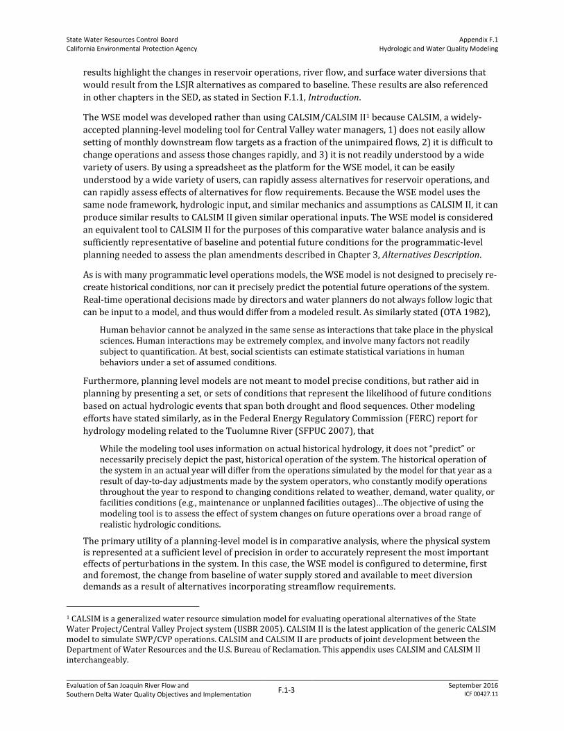
State Water Resources Control Board California Environmental Protection Agency
Appendix F.1 Hydrologic and Water Quality Modeling
Evaluation of San Joaquin River Flow and Southern Delta Water Quality Objectives and Implementation
F.1-3 September 2016
ICF 00427.11
results highlight the changes in reservoir operations, river flow, and surface water diversions that
would result from the LSJR alternatives as compared to baseline. These results are also referenced
in other chapters in the SED, as stated in Section F.1.1, Introduction.
The WSE model was developed rather than using CALSIM/CALSIM II1 because CALSIM, a widely-
accepted planning-level modeling tool for Central Valley water managers, 1) does not easily allow
setting of monthly downstream flow targets as a fraction of the unimpaired flows, 2) it is difficult to
change operations and assess those changes rapidly, and 3) it is not readily understood by a wide
variety of users. By using a spreadsheet as the platform for the WSE model, it can be easily
understood by a wide variety of users, can rapidly assess alternatives for reservoir operations, and
can rapidly assess effects of alternatives for flow requirements. Because the WSE model uses the
same node framework, hydrologic input, and similar mechanics and assumptions as CALSIM II, it can
produce similar results to CALSIM II given similar operational inputs. The WSE model is considered
an equivalent tool to CALSIM II for the purposes of this comparative water balance analysis and is
sufficiently representative of baseline and potential future conditions for the programmatic-level
planning needed to assess the plan amendments described in Chapter 3, Alternatives Description.
As is with many programmatic level operations models, the WSE model is not designed to precisely re-
create historical conditions, nor can it precisely predict the potential future operations of the system.
Real-time operational decisions made by directors and water planners do not always follow logic that
can be input to a model, and thus would differ from a modeled result. As similarly stated (OTA 1982),
Human behavior cannot be analyzed in the same sense as interactions that take place in the physical sciences. Human interactions may be extremely complex, and involve many factors not readily subject to quantification. At best, social scientists can estimate statistical variations in human behaviors under a set of assumed conditions.
Furthermore, planning level models are not meant to model precise conditions, but rather aid in
planning by presenting a set, or sets of conditions that represent the likelihood of future conditions
based on actual hydrologic events that span both drought and flood sequences. Other modeling
efforts have stated similarly, as in the Federal Energy Regulatory Commission (FERC) report for
hydrology modeling related to the Tuolumne River (SFPUC 2007), that
While the modeling tool uses information on actual historical hydrology, it does not “predict” or necessarily precisely depict the past, historical operation of the system. The historical operation of the system in an actual year will differ from the operations simulated by the model for that year as a result of day-to-day adjustments made by the system operators, who constantly modify operations throughout the year to respond to changing conditions related to weather, demand, water quality, or facilities conditions (e.g., maintenance or unplanned facilities outages)…The objective of using the modeling tool is to assess the effect of system changes on future operations over a broad range of realistic hydrologic conditions.
The primary utility of a planning-level model is in comparative analysis, where the physical system is represented at a sufficient level of precision in order to accurately represent the most important effects of perturbations in the system. In this case, the WSE model is configured to determine, first and foremost, the change from baseline of water supply stored and available to meet diversion demands as a result of alternatives incorporating streamflow requirements.
1 CALSIM is a generalized water resource simulation model for evaluating operational alternatives of the State Water Project/Central Valley Project system (USBR 2005). CALSIM II is the latest application of the generic CALSIM model to simulate SWP/CVP operations. CALSIM and CALSIM II are products of joint development between the Department of Water Resources and the U.S. Bureau of Reclamation. This appendix uses CALSIM and CALSIM II interchangeably.

State Water Resources Control Board California Environmental Protection Agency
Appendix F.1 Hydrologic and Water Quality Modeling
Evaluation of San Joaquin River Flow and Southern Delta Water Quality Objectives and Implementation
F.1-4 September 2016
ICF 00427.11
The WSE model is a monthly spreadsheet model that calculates the monthly flows, reservoir storage
levels, and water supply diversions for each eastside tributary based upon user-specified target
flows, other user defined inputs, input from CALSIM II, and flood storage rules. The general
approach is to calculate available water for diversion in each water year based on inflows, net
available water from storage after carryover guidelines, and after streamflow targets are met. User-
defined inputs to the model include the following.
Months for which flow targets are to be set.
Monthly flow targets as a percentage of unimpaired monthly flow for each eastside tributary.
Monthly minimum flows for each eastside tributary.
Minimum annual surface water diversion (can supersede storage guidelines).
Annual end-of-September storage guidelines.
Maximum annual allowable draw2 from reservoirs as a fraction of the available storage.
Other inputs not defined by the user included the following:
CALSIM II inflows to each major reservoir (New Melones, New Don Pedro, and Lake McClure),
and SJR inflow from upstream of the Merced River confluence near Newman.
CALSIM II evaporation rates from each major reservoir
CALSIM II accretions/depletions downstream from each major reservoir including diversions.
CALSIM II Consumptive Use of Applied Water (CUAW) monthly values. Translation from CUAW
to diversion demand was based on updated estimates of district water balance components.
CALSIM II flood storage rule curves at each major reservoir.
The sections below describe the calculation methodologies for flow targets, surface water demands,
diversion deliveries, and the river and reservoir water balances; the development process for the
WSE-CALSIM baseline scenario; and the development of inputs and assumptions for the WSE CEQA
baseline and LSJR alternative simulations. Output data from the WSE model LSJR alternative
simulations, including annual diversions, monthly river flows, and monthly reservoir storage, are
compared to baseline conditions to assess the effects of the LSJR alternatives and intermediate
simulations (i.e., 30 percent and 50 percent unimpaired flow) in Section F.1.2.2, Water Supply Effects
Model Results.
F.1.2.1 U.S. Bureau of Reclamation CALSIM II SJR Module
The WSE model had its origin in the CALSIM II SJR module node framework. The U.S. Bureau of
Reclamation (USBR) developed the CALSIM II SJR module to simulate monthly flows, reservoir
storages, and water supply deliveries in the SJR Basin subject to specific requirements. The module
is part of the larger CALSIM II planning model for the entire Central Valley Project (CVP) and State
Water Project (SWP) that calculates reservoir operations and Delta operations for a specified set of
water resources and level of development (i.e., demands) and regulatory requirements using the
2 Allowable draw in this case refers to a reservoir modeling parameter that determines the available water allocation. This is not intended in a regulatory sense but, rather, to provide an example of reservoir operations to meet both streamflow requirements and carryover storage guidelines and preserve a portion for the following year’s supply as well as maintaining cold pool.

State Water Resources Control Board California Environmental Protection Agency
Appendix F.1 Hydrologic and Water Quality Modeling
Evaluation of San Joaquin River Flow and Southern Delta Water Quality Objectives and Implementation
F.1-5 September 2016
ICF 00427.11
historical sequence of hydrologic conditions 1922–2003. The CALSIM II SJR module encompasses
the SJR Basin from the Upper SJR at Millerton Reservoir to Vernalis, including all tributaries to the
LSJR.
The watershed inflows to Millerton Reservoir, the Fresno and Chowchilla Rivers, and the inflows to
Lake McClure on the Merced River, New Don Pedro Reservoir on the Tuolumne River, and New
Melones Reservoir on the Stanislaus River are the primary boundary conditions of the SJR module.
In the module, these inflows have been modified from the unimpaired runoff by upstream reservoir
operations. The New Melones inflows, developed by USBR, are a combination of planning study
inflows and actual recorded inflows for recent years. The New Don Pedro inflows, provided by CCSF
are a result of a long-term simulation of current project operations for the period prior to 1996 and
actual computed inflow since 1996. The Lake McClure inflows were estimated using the Lake
McClure outflows adjusted for change in storage and evaporation in Lake McClure (USBR 2005).
Subject to the calculated inflows, the CALSIM II SJR module estimates the reservoir operations,
diversions and river flows on each tributary to the LSJR, considering flow requirements, municipal
and agricultural demands, and other operational constraints like flood control. It calculates annual
available river diversions using the end-of-February storage plus actual March–September reservoir
inflow (perfect foresight) on the Stanislaus and Merced Rivers, and March storage plus April–July
reservoir inflows on the Tuolumne River. Flow requirements also factor in to the available
diversions by reducing the amount of surface water available by the volume required to be released.
On the Stanislaus River, the USBR also delivers water to CVP contractors, primarily based on a
lookup table that determines the availability of water as related to the New Melones Index (NMI)
and allows up to a maximum of 155 thousand acre feet (TAF) to be delivered annually.
The State Water Board used the SJR module (USBR 2013a, 2013b) and made minor adjustments to
operations on the Stanislaus River and Vernalis pulse flow requirements. The first Stanislaus
operations adjustment included an updated representation of the National Marine Fisheries Service
(NMFS) Biological Opinion Stanislaus River Reasonable and Prudent Alternative (RPA), including
Action 3.1.3 (NMFS BO) Table 2E flow requirements (i.e., lookup table), which are based on the NMI
(NMFS 2009). The second adjustment was to allow full CVP/SWP diversions (Stockton East Water
District and Central San Joaquin Water Control District) up to 155 TAF/y, if available, by using a
diversion delivery schedule based on the NMI (Table F.1.2-1). The third adjustment (conducted by
USBR) fixed a bug related to the Vernalis pulse flow calculation where, in the DWR 2009 Delivery
Reliability Report, flows had overestimated the pulse volumes in April and May. The last adjustment
to the Stanislaus operations was to begin the model with a New Melones Reservoir starting storage
of 1,000,000 acre-feet (AF) on October 1, 1922, instead of 1,700,000 AF.
Table F.1.2-1. Stanislaus River Combined CVP Contractor (Stockton East Water District [SEWD] and Central San Joaquin Water Conservation District [CSJWCD]) Diversion Delivery Curves Based on New Melones Index Used in the WSE Model
New Melones Index (TAF) SEWD Delivery (TAF) CSJWCD Delivery (TAF) Total (TAF)
> 1,800 75 80 155
1,400–1,800 10 49 59
0–1,400 10 0 10

State Water Resources Control Board California Environmental Protection Agency
Appendix F.1 Hydrologic and Water Quality Modeling
Evaluation of San Joaquin River Flow and Southern Delta Water Quality Objectives and Implementation
F.1-6 September 2016
ICF 00427.11
The State Water Board CALSIM case includes the D-1641 base flow and salinity objective at Vernalis
to be released from New Melones Reservoir. The VAMP April 15–May 15 Vernalis pulse flows are
released based on the San Joaquin River Agreement (SJRA) distribution schedule from either New
Melones Reservoir, New Don Pedro Reservoir, or Lake McClure. In the State Water Board CALSIM
case, other than VAMP pulse flows, the minimum flows on the Tuolumne and Merced River were
based on the current requirements by FERC, the Davis-Grunsky Agreement, CDFW Settlement
Agreement for the Tuolumne River, and the Cowell Agreement. This model version did not include
San Joaquin River Restoration Program (SJRRP) flow releases.
Appendix C, Technical Report on the Scientific Basis for Alternative San Joaquin River Flow and
Southern Delta Salinity Objectives, contains an analysis of historical SJR flow and salinity. It compares
measured monthly average SJR flows at Vernalis with the CALSIM results for water years 1984–
2003. This covers a period during which actual operations in the watershed were relatively similar
to those modeled in the CALSIM representation of current conditions. All major eastside dams were
completed and filled, and their combined effect on flows at Vernalis is present in the actual data.
CALSIM model output ends with water year 2003. The comparison of CALSIM results with recent
historical flow and EC (salinity) data demonstrates that it provides a reasonable (accurate)
representation of the baseline SJR flow and EC conditions.
F.1.2.2 Development of the WSE Model Baseline and Alternative Assumptions
This section contains the assumptions and methods used to develop the WSE model baseline and
Alternative scenarios. In addition, this section also describes the static inputs to the calculations
above.
The WSE model baseline conditions were developed such that they would corroborate with
CALSIM II SJR module results, both subject to a similar set of assumptions and rules and, thus,
demonstrating the efficacy of the WSE model. The State Water Board conducted CALSIM II modeling
using the CALSIM II SJR module supplied by USBR (USBR 2013a, 2013b). This version of the model
contained many of the same assumptions and inputs as the CALSIM II “Current Conditions” case
used in the DWR 2009 Delivery Reliability Report (DWR 2010), a version of CALSIM II which closely
represents the baseline conditions over 82 years of historical climate. Differences between CALSIM
II and the WSE model are described below.
CALSIM was used for corroboration because it is a widely accepted and rigorously reviewed
planning model for the Central Valley, and contains a longer available dataset for comparison than
historical data alone. Furthermore, as the observed historical conditions become increasingly
different than current conditions reaching farther back in history, corroboration with a baseline
conditions model becomes more appropriate than calibration to historical data.
The WSE CALSIM-baseline results set is the baseline WSE model run that best matches CALSIM II
levels of demand and water balance parameters, while the WSE CEQA-baseline incorporates
adjusted levels of demand and water balance parameters based on the best available information,
including recent published data from Agricultural Water Management Plans.
The WSE CEQA-baseline version was developed to better model baseline conditions representative
of the 2009 existing environment, and most consistent with the definition of baseline conditions.
The primary changes from WSE CALSIM-baseline to WSE CEQA-baseline were related to estimates

State Water Resources Control Board California Environmental Protection Agency
Appendix F.1 Hydrologic and Water Quality Modeling
Evaluation of San Joaquin River Flow and Southern Delta Water Quality Objectives and Implementation
F.1-7 September 2016
ICF 00427.11
of demand as described in Tables F.1.2-12, F.1.2-13, and F.1.2-15. In addition, the level of Merced
Cowell Agreement diversions is changed from CALSIM levels to full diversion according to
Table F.1.2-7. The only other difference is that under CALSIM mode the Stanislaus minimum
monthly flow requirement given in Table F.1.2-4 is chosen based on NMI calculated from the
CALSIM Storage levels, while under CEQA-baseline the storage is calculated from equation F.1-8.
Figure F.1.2-1 illustrates the relationship between SWRCB-CALSIM II, WSE model with CALSIM
parameters for corroboration purposes, and WSE model CEQA-baseline used for alternatives
analysis.
Figure F.1.2-1. Illustration of Differing Model Configurations Described in This Appendix
Table F.1.2-2, below, describes the differences in baseline assumptions for DWR DRR 2009
CALSIM II, USBR CALSIM II, the adapted version referred to herein as SWRCB-CALSIM II, and WSE
baseline (used in this recirculated SED analysis). Based on comments received on the 2012 Draft
SED and further study, the 2012 Draft SED WSE model has been revised, as described in Table F.1.2-
3.

State Water Resources Control Board California Environmental Protection Agency
Appendix F.1 Hydrologic and Water Quality Modeling
Evaluation of San Joaquin River Flow and Southern Delta Water Quality Objectives and Implementation
F.1-8 September 2016
ICF 00427.11
Table F.1.2-2. DWR DRR CALSIM II, USBR CALSIM II, SWRCB CALSIM II, and WSE Baseline Model Assumptions
CALSIM II and Baseline Model Assumptions
DWR DRR CALSIM II (used for 2012 Draft SED baseline) USBR CALSIM II SWRCB CALSIM II WSE – Baselinea
Diversion Delivery Method
Stan: Feb storage plus Mar–Sep inflow
Tuol: Mar storage plus Apr–Jul inflow
Mer: Mar storage plus Apr–Sep inflow
Unchanged Unchanged Index of March 1 storage plus Apr–Sep inflow with WSE allocation scheme
SJRRP Not Included Included Not included Not included
VAMP and VAMP Base
Included – double step with split responsibility based on schedule
Included – single step, Merced fully responsible
Included – double step with split responsibility based on schedule
Included – double step with split responsibility(uses CALSIM VAMP pulse flow values)
D-1641 Base Flow (including X2) Feb–Jun
Included Included Included Included
D-1641 Pulse Flow (including X2) Apr–May
Not Included Not Included Not included (VAMP instead)
Not included
(VAMP instead)
D-1641 Vernalis EC (12 months)
Included Included Included Included
New Melones Starting Storage
1,000 TAF 1,700 TAF 1,000 TAF 1,000 TAF
Stanislaus Minimum Flows Stanislaus RPA
Included – although has errors Included – errors fixed (contains off-ramp in drought sequence)
Included – errors fixed (no off-ramp)b
Included – errors fixed (no off-ramp)b
Tuolumne Minimum Flows 1995 FERC
Included Included Included Included
Merced Minimum Flows
Davis-Grunsky/FERC/Cowell Davis-Grunsky/ FERC/Cowell
Davis-Grunsky/FERC/Cowell
Davis-Grunsky/ FERC/Cowell

State Water Resources Control Board California Environmental Protection Agency
Appendix F.1 Hydrologic and Water Quality Modeling
Evaluation of San Joaquin River Flow and Southern Delta Water Quality Objectives and Implementation
F.1-9 September 2016
ICF 00427.11
CALSIM II and Baseline Model Assumptions
DWR DRR CALSIM II (used for 2012 Draft SED baseline) USBR CALSIM II SWRCB CALSIM II WSE – Baselinea
Stanislaus Annual Irrigation Year (Mar–Feb) Diversions from 1922 to 2003
2005 level of development
Max ~560 TAF SSJID/OID
+ Max ~117 TAF SEWD/CSJWCD
+ ~20 TAF Riparian
2020 level of development
Max ~590 TAF SSJID/OID
+ Max ~155 TAF SEWD/CSJWCD
+ ~20 TAF Riparian
2020 level of development
Max ~590 TAF SSJID/OID
+ Max ~155 TAF SEWD/CSJWCD
+ ~20 TAF Riparian
CALSIM LOD2020/modified
Max ~594 TAF SSJID/OID
+ Max ~155 TAF SEWD/CSJWCD
+ ~20 TAF Riparian
Tuolumne Annual Irrigation Year (Mar–Feb) Diversions from 1922 to 2003
2005 level of development Max ~1,094 TAF MID/TID
+ ~8 TAF Riparian
2020 level of development
Max ~1,107 TAF MID/TID
+ ~7 TAF Riparian
2020 level of development
Max ~1,107 TAF MID/TID
+ ~7 TAF Riparian
CALSIM LOD2020/modified
Max ~1,025 TAF MID/TID
+ ~7 TAF Riparian
Merced Annual Irrigation Year (Mar–Feb) Diversions from 1922 to 2003
2005 level of development
Max ~543 TAF Merced ID
+ ~26 TAF Cowell
+ ~41 TAF Riparian
2020 level of development
Max ~528 TAF Merced ID
+ ~25 TAF Cowell
+ ~41 TAF Riparian
2020level of development
Max ~528 TAF Merced ID
+ ~25 TAF Cowell
+ ~41 TAF Riparian
CALSIM LOD2020/modified
Max ~542 TAF Merced ID
+ ~94 TAF Cowell
+ ~41 TAF Riparian
Operational Maximum Flowc
1,500 cubic feet per second (cfs) in Stanislaus River
Stan max flow removed
Stan max flow removed 9,999 cfs on all three tributaries
a. All of these parameters are equivalent in WSE versions described as “WSE-CALSIM baseline” and “WSE-CEQA baseline,” with the exception of the adjustment factors for CUAW demand.
b. The RPA used in modeling is based on the NMI, and thus, as the cumulative distribution of storage changes, so would the RPA required flow (can potentially be different within the alternatives). c. Flow maximum may be exceeded in spill events for flood control.
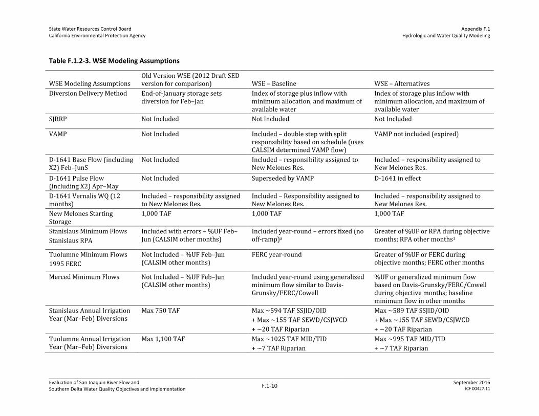
State Water Resources Control Board California Environmental Protection Agency
Appendix F.1 Hydrologic and Water Quality Modeling
Evaluation of San Joaquin River Flow and Southern Delta Water Quality Objectives and Implementation
F.1-10 September 2016
ICF 00427.11
Table F.1.2-3. WSE Modeling Assumptions
WSE Modeling Assumptions Old Version WSE (2012 Draft SED version for comparison) WSE – Baseline WSE – Alternatives
Diversion Delivery Method End-of-January storage sets diversion for Feb–Jan
Index of storage plus inflow with minimum allocation, and maximum of available water
Index of storage plus inflow with minimum allocation, and maximum of available water
SJRRP Not Included Not Included Not Included
VAMP Not Included Included – double step with split responsibility based on schedule (uses CALSIM determined VAMP flow)
VAMP not included (expired)
D-1641 Base Flow (including X2) Feb–JunS
Not Included Included – responsibility assigned to New Melones Res.
Included – responsibility assigned to New Melones Res.
D-1641 Pulse Flow (including X2) Apr–May
Not Included Superseded by VAMP D-1641 in effect
D-1641 Vernalis WQ (12 months)
Included – responsibility assigned to New Melones Res.
Included – Responsibility assigned to New Melones Res.
Included – responsibility assigned to New Melones Res.
New Melones Starting Storage
1,000 TAF 1,000 TAF 1,000 TAF
Stanislaus Minimum Flows
Stanislaus RPA
Included with errors – %UF Feb–Jun (CALSIM other months)
Included year-round – errors fixed (no off-ramp)a
Greater of %UF or RPA during objective months; RPA other months1
Tuolumne Minimum Flows
1995 FERC
Not Included – %UF Feb–Jun (CALSIM other months)
FERC year-round Greater of %UF or FERC during objective months; FERC other months
Merced Minimum Flows Not Included – %UF Feb–Jun (CALSIM other months)
Included year-round using generalized minimum flow similar to Davis-Grunsky/FERC/Cowell
%UF or generalized minimum flow based on Davis-Grunsky/FERC/Cowell during objective months; baseline minimum flow in other months
Stanislaus Annual Irrigation Year (Mar–Feb) Diversions
Max 750 TAF Max ~594 TAF SSJID/OID
+ Max ~155 TAF SEWD/CSJWCD
+ ~20 TAF Riparian
Max ~589 TAF SSJID/OID
+ Max ~155 TAF SEWD/CSJWCD
+ ~20 TAF Riparian
Tuolumne Annual Irrigation Year (Mar–Feb) Diversions
Max 1,100 TAF Max ~1025 TAF MID/TID
+ ~7 TAF Riparian
Max ~995 TAF MID/TID
+ ~7 TAF Riparian

State Water Resources Control Board California Environmental Protection Agency
Appendix F.1 Hydrologic and Water Quality Modeling
Evaluation of San Joaquin River Flow and Southern Delta Water Quality Objectives and Implementation
F.1-11 September 2016
ICF 00427.11
WSE Modeling Assumptions Old Version WSE (2012 Draft SED version for comparison) WSE – Baseline WSE – Alternatives
Merced Annual Irrigation Year (Mar–Feb) Diversions
Max 625 TAF (only 2 years CALSIM diverted up to 625)
Max ~542 TAF Merced ID
+ ~94 TAF Cowell
+ ~41 TAF Riparian
Max ~532 TAF Merced ID
+ ~94 TAF Cowell
+ ~41 TAF Riparian
Flood Storage Curve Stanislaus: same as CALSIM; Tuolumne: does not factor in conditional storage; Merced: greater storage capacity in July–September than CALSIM)
Stanislaus: same as CALSIM Tuolumne: Same as CALSIM (conditional time series) Merced: Same as CALSIM
Stanislaus: same as CALSIM Tuolumne: Same as CALSIM
(conditional time series) Merced: Same as CALSIM
Channel Maximum Flows 2,500 cubic feet per second (cfs); 3,500 cfs; 2,000 cfs
9,999 cfs; 9,999 cfs; 9,999 cfs 9,999 cfs; 9,999 cfs; 9,999 cfs
a. The RPA used in modeling is based on the NMI, and thus, as the cumulative distribution of storage changes, so would the RPA required flow (could be quite different for the alternatives).

State Water Resources Control Board California Environmental Protection Agency
Appendix F.1 Hydrologic and Water Quality Modeling
Evaluation of San Joaquin River Flow and Southern Delta Water Quality Objectives and Implementation
F.1-12 September 2016
ICF 00427.11
Modifications were incorporated into the original WSE modeling based on public comments
received on the 2012 Draft SED. These modifications can be summarized as follows:
CALSIM representation of baseline is no longer used directly in the SED. The WSE model was
modified to provide a representation of baseline conditions, and is now used to model both the
baseline and the LSJR alternatives for the purpose of impacts analysis in the SED. The WSE
model representation of baseline includes the assumptions listed below, and except for the
VAMP minimum flow requirements (first item below), all the other assumptions apply to the
WSE modeling of the LSJR alternatives as well.
o Vernalis Adaptive Management Plan (VAMP) minimum flow requirements per the San
Joaquin River Agreement (USBR and SJRGA 1999 [EIS/EIR for SJRA]).
o Stanislaus RPA 3.1.3 minimum streamflows at Goodwin Dam required by Biological Opinion
Table 2E as a function of NMI (NMFS 2009)
o Stanislaus River maximum diversions based on a 155 TAF total for SEWD and CSJWCD
(USBR 2013a; USBR 2013b) and 600 TAF for SSJID and OID per the 1988 Stipulated
Agreement with USBR (USBR and OID 1988).
o The model no longer waives the minimum February–June percentage of unimpaired flow
requirements during high flow events.
o Future anticipated San Joaquin River Restoration Program flows are not included.
The WSE model now also calculates flow in each tributary for the months of July–January, as
opposed to relying on CALSIM output for those months as was done in the 2012 Draft SED, in
addition to the February–June period. These flows are based on the minimum flow
requirements applicable to each tributary and Vernalis, plus any reservoir releases needed to
maintain compliance with flood storage curves. The model still, however, uses estimates of
reservoir inflows, downstream accretions and depletions, demands, and other inputs as
developed by USBR for the CALSIM model.
WSE modeling of the LSJR alternatives in the 2012 Draft SED was configured to closely match the
baseline condition of end-of-September storage levels in the main reservoirs on each tributary. To
better simulate diversion priorities and reservoir operations, the modified WSE model now
calculates the amount of water available for diversion each year based on the sum of available
end-of-February storage plus March–September inflows (using foresight), less the sum of March–
September river flow requirements and end-of-September minimum storage guidelines (the latter
subject to annual diversion minimum constraints that supersede the guidelines in times of major
shortage). Available water is then compared against estimates of demand (primarily agricultural
irrigation) for the year, with the lesser determining the amount diverted.
Minimum end-of- September storage guidelines storage conditions that maintain coldwater
reserves adequate to ensure there are no temperature-related impacts on fisheries resulting from
lower reservoir levels due to project alternatives. These minimum storage guidelines were
modeled to be waived if certain minimum levels of diversion could not be met, as described in the
below section, Calculation of Available Water for Diversion. Diversion demands for major
irrigation districts are derived from annually- and monthly-varying CUAW demands from CALSIM,
with operational efficiency estimates derived from Agricultural Water Management Plans
(AWMPs), and total diversion and use adjusted for best match to AWMP surface water use data
and district operations models. For smaller diversions, CALSIM values for diversions are used
directly.

State Water Resources Control Board California Environmental Protection Agency
Appendix F.1 Hydrologic and Water Quality Modeling
Evaluation of San Joaquin River Flow and Southern Delta Water Quality Objectives and Implementation
F.1-13 September 2016
ICF 00427.11
With all of the above revisions, and by adjusting the overall demands for each river, the WSE
model was calibrated for best match to SWRCB CALSIM baseline diversions, streamflows, and
reservoir levels. This exercise demonstrated the WSE model’s effectiveness in representing
system dynamics similarly to the CALSIM model.
Next, some water budget quantities in the WSE model were improved based on published
estimates of reservoir losses, municipal and industrial water use, and other factors described in
Appendix F.1. The final WSE baseline used in alternatives analysis includes all of the above
changes, but with additional revisions to improved parameters. This is denoted as “CEQA Mode,”
and differs slightly from the original CALSIM baseline.
In some water year types, a portion of LSJR alternative instream flow requirement was “shifted”
outside of the February–June period to summer or fall months in order to reduce further any
temperature impacts in those months caused by lower reservoir levels.
Maximum streamflows (aka “flow caps”) in downstream reaches were removed from the WSE
model.
F.1.2.3 Calculation of Flow Targets
Generally, the WSE model calculates monthly flow targets for each eastside tributary based on the
existing regulatory minimum flow schedules or user-specified percent of unimpaired monthly flow.
The percentage of unimpaired flow could be variable between tributaries and months, although
uniform values (20, 40, and 60 percent unimpaired flow) were used for each of the tributaries and
for each month for the LSJR alternatives. Monthly unimpaired flows for water years 1922–2003
available from the Department of Water Resources (DWR 2007) are estimates of unimpaired flows
upstream of the major reservoirs. These DWR estimates of unimpaired flows were used as
unimpaired flow indices for the entirety of each eastside tributary because there are no estimates of
unimpaired inflow to the tributaries between the major reservoirs and the LSJR, where the flow
objectives are being established. Furthermore, based on information from DWR (DWR 2007), the
entire Central Valley floor component of unimpaired flow (i.e., downstream of the major reservoirs)
is roughly 3 percent of the unimpaired flows of the three eastside tributaries; thus, the component of
unimpaired flow that would otherwise be associated with accretions and other inputs downstream
of the major reservoirs is not expected to significantly alter the amount or timing of these flows. The
unimpaired flows at the major reservoirs are therefore considered adequate for the purpose of
establishing flow objectives. Proposed percentages of unimpaired flow are considered an additional
requirement, and thus the greater of either the baseline flow requirements or the unimpaired flow
requirement was selected for each month.
The February–June minimum instream flow requirement is calculated as a percentage of that
month’s unimpaired flow, for each month in February–June. For example, the unimpaired flow
volume in the Stanislaus River in February 2003 was 55 TAF. An unimpaired flow of 40 percent
would be 22 TAF (a monthly average of 396 cfs) for the month of February. Each month is calculated
individually. Higher flows such as flood spills would meet the requirement during the month of the
spills, but the surplus would not apply to successive months that would still need to meet the
minimum flow.
The model allows for specifying maximum and minimum monthly flows for each eastside tributary
and at Vernalis. Maximum flows could be selected to limit flooding effects and reduce water supply
effects from extremely high target flows. However, for baseline and the alternatives, there were no
maximum flow levels specified in the WSE model. The minimum monthly flows for each alternative

State Water Resources Control Board California Environmental Protection Agency
Appendix F.1 Hydrologic and Water Quality Modeling
Evaluation of San Joaquin River Flow and Southern Delta Water Quality Objectives and Implementation
F.1-14 September 2016
ICF 00427.11
and the baseline have been set to the existing (baseline) regulatory minimum flow requirements
within each tributary. These existing flow requirements generally apply to the release of flows at the
re-regulating or diversion dams on the Stanislaus, Tuolumne, and the Merced Rivers (Goodwin Dam,
La Grange Dam, and Crocker Huffman Dam, respectively), while the WSE model sets flow
requirements at the confluences with the LSJR. Minimum flow requirements at the confluences were
determined by translating the existing upstream requirements using CALSIM accretions and
depletions of flow between the dams and downstream. This allows for meeting existing requirements
upstream while also allowing the unimpaired flow requirements to be specified near the confluences.
On the Stanislaus River, the existing minimum flow requirement is from the 2009 National Marine
Fisheries Service (NMFS) biological opinion (BO) Stanislaus River Reasonable and Prudent
Alternatives (RPAs), including Action 3.1.3 (NMFS 2009). These flows have been interpreted as
monthly flow totals by the WSE model as shown in Table F.1.2-4, preserving the total volumes and
including pulse flows. The schedule was based on the NMI, (a value set each year as the March 1
storage plus projected inflows to the New Melones Reservoir through September). The WSE model
calculates the NMI each year as the end-of-February storage in New Melones plus the total of
anticipated New Melones inflow March–September (available water supply through the end of the
water year). New Melones inflows, an input to CALSIM II, are a combination of planning study
inflows and actual recorded inflows for recent years (USBR 2004). As this flow schedule is
dependent on storage, changes in storage relative to baseline result in changes to the flow
requirement relative to baseline.
Table F.1.2-4. Minimum Monthly Flow Requirements at Goodwin Dam on the Stanislaus River per NMFS BO Table 2E
New Melones Index
Minimum Monthly Flow (TAF) by New Melones Index
> 3,000 > 2,500 > 2,000 > 1,400 > 0
Calendar Month
1 22 14.3 13.9 13.5 13.1
2 20.2 13.1 13.1 12.3 11.9
3 101.2 93.4 12.3 12.3 12.3
4 97 83.2 92.3 45.5 27.3
5 120.2 95.4 76.2 38.7 24.6
6 65.3 55.8 21.6 11.9 8.9
7 26.3 18.4 15.3 12.3 9.2
8 24.6 18.4 15.3 12.3 9.2
9 23.8 17.8 14.9 11.9 8.9
10 51.7 48.9 47.5 34.8 35.8
11 17.8 11.9 11.9 11.9 11.9
12 18.4 12.3 12.3 12.3 12.3
Annual 588.5 482.8 346.5 229.6 185.3
Notes:
Sum of daily values in Appendix 2E of NMFS BO (NMFS 2009).
New Melones Index is the sum of March 1st Storage in New Melones plus projected inflow through September.
TAF = thousand acre feet per month

State Water Resources Control Board California Environmental Protection Agency
Appendix F.1 Hydrologic and Water Quality Modeling
Evaluation of San Joaquin River Flow and Southern Delta Water Quality Objectives and Implementation
F.1-15 September 2016
ICF 00427.11
On the Tuolumne River, the existing minimum flow requirement is the 1995 FERC minimum flow
requirement at La Grange Dam established in 1995 by Article 37 of the FERC license (Project
Number 2299) in the settlement agreement between USBR and the California Department of Fish
and Wildlife (CDFW). Table F.1.2-5 contains the monthly flow schedule as interpreted by the WSE
model by water year type. As this is a total monthly flow, the pulse flows are retained in the monthly
volumes. The schedule uses the SJR 60-20-20 water year type index, as defined by Water Rights
Decision D-1641 (SWRCB 2000). The WSE model uses the historical water year type Water Supply
Indices to determine the required flows in any given year over the 82-year model sequence.
Table F.1.2-5. Minimum Monthly Flow Requirements at La Grange Dam on the Tuolumne River per 1995 FERC Settlement Agreement
Index
Minimum Monthly Flow (TAF) by San Joaquin Basin (60-20-20) Water Year Type Index
> 3,100 > 2,700 > 2,400 > 2,200 > 2,000 > 1,500 > 0
Calendar Month
1 18.4 10.8 11.1 9.2 9.2 9.2 9.2
2 16.7 9.7 10.0 8.3 8.3 8.3 8.3
3 18.4 10.8 11.1 9.2 9.2 9.2 9.2
4 63.1 40.6 28.8 27.6 25.4 19.1 14.6
5 63.1 40.6 28.8 27.6 25.4 19.1 14.6
6 14.9 4.5 4.5 4.5 3.0 3.0 3.0
7 15.4 4.6 4.6 4.6 3.1 3.1 3.1
8 15.4 4.6 4.6 4.6 3.1 3.1 3.1
9 14.9 4.5 4.5 4.5 3.0 3.0 3.0
10 24.4 13.2 12.7 9.2 9.2 7.7 7.7
11 17.9 10.4 10.7 8.9 8.9 8.9 8.9
12 18.4 10.8 11.1 9.2 9.2 9.2 9.2
Annual 300.9 165.0 142.5 127.5 117.0 103.0 94.0
Notes:
Monthly interpretation of 1995 FERC Settlement Agreement including pulse flows (FERC 1995).
San Joaquin Valley water year type index (60-20-20) as defined by D-1641 (SWRCB 2000).
TAF = thousand acre-feet per month
On the Merced River, the existing minimum flow requirement is a combination of the FERC (Project
Number 2179) requirements and the 1967 Davis-Grunsky Contract (DWR 1967). Table F.1.2-6
contains the WSE model interpretation of the minimum flow requirement. To develop Merced River
minimum flows in the WSE model, the highest of the FERC or Davis-Grunsky flows in a given month
is selected and assumed to be the same in all years. The “normal year” FERC schedule is used to
simplify the requirement between Normal and Dry. An additional release of 12,500 AF in October
was also required on top of the FERC minimum flow requirement to satisfy the CDFW fall fishery
pulse flow requirement. The Cowell Agreement Diversion (CAD) release requirements, presented in
Table F.1.2-7, are not factored into the flow target, but they are included in release and diversion
requirements discussed below. CAD releases are released from Crocker-Huffman Dam, but are
entirely diverted, and do not contribute to minimum flows at the confluence with the LSJR.

State Water Resources Control Board California Environmental Protection Agency
Appendix F.1 Hydrologic and Water Quality Modeling
Evaluation of San Joaquin River Flow and Southern Delta Water Quality Objectives and Implementation
F.1-16 September 2016
ICF 00427.11
Table F.1.2-6. Minimum Monthly Flow Requirements and Modeled Flow Requirement at Shaffer Bridge on the Merced River per FERC 2179 License, Article 40 and 41
FERC (cfs) FERC (cfs) Davis-Grunsky (cfs) Davis-Grunsky (cfs) Modeled (cfs)
Calendar Month Normal Year Dry Year Normal Year Dry Year All Years1
1 75 60 220 180 220
2 75 60 220 180 220
3 75 60 220 180 220
4 75 60
No
t A
pp
lica
ble
No
t A
pp
lica
ble
75
5 75 60 75
6 25 15 25
7 25 15 25
8 25 15 25
9 25 15 25
10 50 38 2801
11 100 75 220 180 220
12 100 75 220 180 220
Notes:
For simplification, and due to inconsistencies with CALSIM II, Normal Year minimum flows on the Merced River were assumed for all years. 1 Includes additional CDFW fall fishery release of 12,500 acre-feet in October.
cfs = cubic feet per second (monthly average)
Table F.1.2-7. Monthly Cowell Agreement Diversions on the Merced River between Crocker-Huffman Dam and Shaffer Bridge
Calendar Month Modeled Cowell Agreement Release (cfs)
1 50
2 50
3 100
4 175
5 225
6 250
7 225
8 175
9 150
10 50
11 50
12 50
Annual (TAF) 94
Notes:
Cowell Agreement release assumed to be fully released by Merced Irrigation District at Crocker-Huffman Dam and fully diverted before Shaffer Bridge.
TAF = thousand acre-feet per month; cfs = cubic feet per second

State Water Resources Control Board California Environmental Protection Agency
Appendix F.1 Hydrologic and Water Quality Modeling
Evaluation of San Joaquin River Flow and Southern Delta Water Quality Objectives and Implementation
F.1-17 September 2016
ICF 00427.11
Two factors result in releases that may be different from the unimpaired flow objectives. The first is
that the model calculates and releases additional flow, as described below, when required to
maintain reservoirs below CALSIM flood control storage requirements, also known by the general
term “spill.” The second, as described in Appendix K, Revised Water Quality Control Plan, is that as
part of adaptive implementation, flows can be shifted outside of the February–June period and into
the summer and fall to provide for temperature control, to reduce likelihood of negative effects, and
to increase the overall potential benefit. This flow shift, described in further detail later in this
appendix, is not part of the unimpaired flow objective. However, the calculation in the modeling
attenuates the target volume by the amount to be shifted and increases July–November flows by
increasing the minimum flow target. Because of these adjustments, the WSE model calculates flows
that can be lower or higher than the specified percent of unimpaired flow or minimum flow.
As described above, the flow target at the mouth of each eastside tributary, QFt, for a particular
month, t, is calculated as:
𝑄𝐹𝑡 = 𝑀𝑖𝑛(𝑀𝑎𝑥 𝑈𝐹𝑡 ∗ 𝐹𝑎𝑡 , 𝑄𝑚𝑛𝑡 ,𝑄𝑚𝑥𝑡) (Eqn. F.1-1)
Where:
UFt is the DWR monthly unimpaired flow for month t (DWR 2007);
Fat is the monthly target percentage of unimpaired flow defined by the user; and
Qmxt and Qmnt are the user defined maximum and minimum regulatory defined monthly flows,
for month t. In any given month, the flow target is the highest target set for that month (e.g., if
percent of unimpaired flow was lower than the minimum, the minimum would be the target).
If flows are to be shifted outside of the February–June period, QFt is adjusted accordingly.
With the flow target defined, WSE then performs an initial flow routing on each tributary prior to
making any releases from the rim dams. This routing takes into account any accretions/depletion,
stream inflows, non-district and non-riparian diversions, and return flows that occur before the
confluence with the San Joaquin River. These inflow timeseries are taken directly from CALSIM II.
Since this routing is intended to identify how each tributary is affected by the CALSIM II inflow
timeseries, the flow may be negative. If any negative flows are found, the tributary’s rim dam must
release enough water to eliminate them. Depending on the location of the negative flow along the
tributary this release may count towards any flow requirements upstream. From here WSE operates
the rim dams to meet the flow target defined above. First, WSE releases enough water to meet the
unimpaired flow requirement at the confluence for the February–June period. Second, WSE releases
water to meet each tributaries minimum flow requirement at the downstream regulating reservoirs
(Crocker-Huffman, La Grange, and Goodwin) in all months, unless it was already satisfied with one
of the previous releases. Finally, WSE makes any flow shifting releases. On the Merced River there is
also an additional release on top of the others to meet the Cowell Agreement flow requirement at
Crocker Huffman.
The WSE model also contains a user-defined flow target for the SJR at Vernalis that, if not met by the
tributary releases, requires additional releases to meet the Vernalis minimum. The user may select
among D-1641 pulse and base flow and salinity at Vernalis, VAMP pulse flows, and/or a user defined
minimum to be met at Vernalis. Tables F.1.2-8 and F.1.2-9 contain the D-1641 and VAMP Vernalis
flow schedules as interpreted by the WSE model. When activated in the model, the D-1641 pulse and
base flows and salinity only require additional releases from the Stanislaus River. Additional pulse

State Water Resources Control Board California Environmental Protection Agency
Appendix F.1 Hydrologic and Water Quality Modeling
Evaluation of San Joaquin River Flow and Southern Delta Water Quality Objectives and Implementation
F.1-18 September 2016
ICF 00427.11
flows to meet VAMP, if activated, were distributed to each tributary according to Table F.1.2-10. The
user-defined minimum at Vernalis distributes any additional flow, if needed, to each of the three
eastside tributaries based on their unimpaired flow contribution as 29, 47, and 24 percent from the
Stanislaus, Tuolumne, and Merced Rivers respectively. The Vernalis flow and water quality
requirements are discussed in more detail in Appendix C, Technical Report on the Scientific Basis for
Alternative San Joaquin River Flow and Southern Delta Salinity Objectives.
Table F.1.2-8. D-1641 Minimum Monthly Flow Requirements and Maximum Salinity Concentration in the SJR at Airport Way Bridge Near Vernalis
Calendar Month Minimum Monthly Flow (TAF) by San Joaquin River
Basin (60-20-20) Water Year Type Maximum Salinity
Concentration
60-20-20 Water Year Type2
Feb 1–April 14 and May 16–June 301 (cfs)
April 15–May 151
(cfs) October
(cfs) April–Aug
(mmhos/cm) Sep–March
(mmhos/cm)
W 2,130/3,420 7,330/8,620 2,000 0.7 1.0
AN 2,130/3,420 5,730/7,020 2,000 0.7 1.0
BN 1,420/2,280 4,620/5,480 2,000 0.7 1.0
D 1,420/2,280 4,020/4,880 2,000 0.7 1.0
C 710/1,140 3,110/3,540 2,000 0.7 1.0
Notes: 1 Greater flow used when required X2 position is at or west of Chipps Island (km 75). The required X2 position was determined by CALSIM and used in the WSE for each alternative and the baseline. The X2 standard, introduced in the 1995 Bay-Delta Plan, refers to the position at which 2 parts per thousand (ppt) salinity occurs in the Delta estuary and is designed to improve shallow-water fish habitat in the spring of each year and can limit export pumping. 2 San Joaquin Valley Water Year Type Index (60-20-20) as defined by D-1641 (SWRCB 2000).
cfs = cubic feet per second
mmhos/cm = millimhos per centimeter
W = wet
AN = above normal
BN = below normal
D = dry
C = critically dry
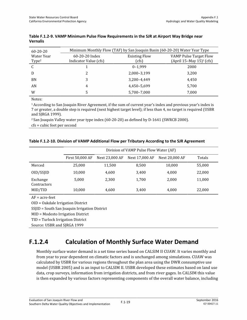
State Water Resources Control Board California Environmental Protection Agency
Appendix F.1 Hydrologic and Water Quality Modeling
Evaluation of San Joaquin River Flow and Southern Delta Water Quality Objectives and Implementation
F.1-19 September 2016
ICF 00427.11
Table F.1.2-9. VAMP Minimum Pulse Flow Requirements in the SJR at Airport Way Bridge near Vernalis
60-20-20 Water Year Type2
Minimum Monthly Flow (TAF) by San Joaquin Basin (60-20-20) Water Year Type
60-20-20 Index Indicator Value (cfs)
Existing Flow (cfs)
VAMP Pulse Target Flow (April 15–May 15)1 (cfs)
C 1 0–1,999 2000
D 2 2,000–3,199 3,200
BN 3 3,200–4,449 4,450
AN 4 4,450–5,699 5,700
W 5 5,700–7,000 7,000
Notes: 1 According to San Joaquin River Agreement, if the sum of current year’s index and previous year’s index is 7 or greater, a double step is required (next highest target level); if less than 4, no target is required (USBR and SJRGA 1999). 2 San Joaquin Valley water year type index (60-20-20) as defined by D-1641 (SWRCB 2000).
cfs = cubic feet per second
Table F.1.2-10. Division of VAMP Additional Flow per Tributary According to the SJR Agreement
Division of VAMP Pulse Flow Water (AF)
First 50,000 AF Next 23,000 AF Next 17,000 AF Next 20,000 AF Totals
Merced 25,000 11,500 8,500 10,000 55,000
OID/SSJID 10,000 4,600 3,400 4,000 22,000
Exchange Contractors
5,000 2,300 1,700 2,000 11,000
MID/TID 10,000 4,600 3,400 4,000 22,000
AF = acre-feet
OID = Oakdale Irrigation District
SSJID = South San Joaquin Irrigation District
MID = Modesto Irrigation District
TID = Turlock Irrigation District
Source: USBR and SJRGA 1999
F.1.2.4 Calculation of Monthly Surface Water Demand
Monthly surface water demand is a set time series based on CALSIM II CUAW. It varies monthly and
from year to year dependent on climatic factors and is unchanged among simulations. CUAW was
calculated by USBR for various regions throughout the plan area using the DWR consumptive use
model (USBR 2005) and is an input to CALSIM II. USBR developed these estimates based on land use
data, crop surveys, information from irrigation districts, and from river gages. In CALSIM this value
is then expanded by various factors representing components of the overall water balance, including
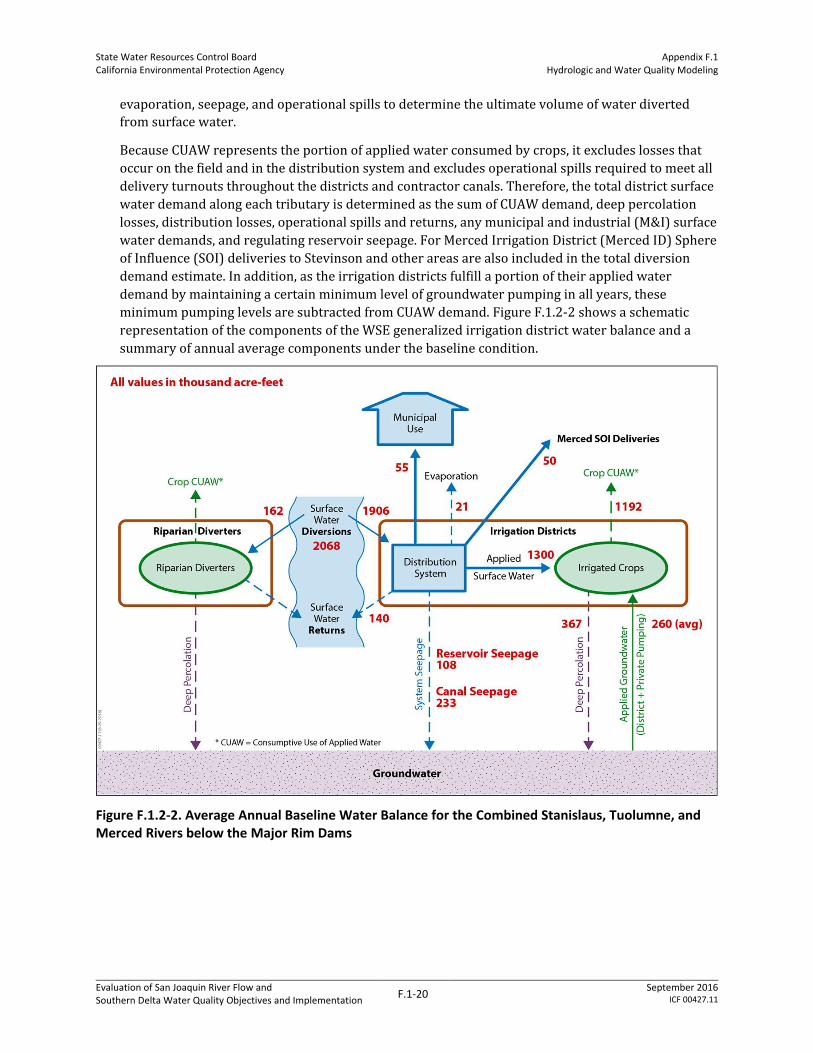
State Water Resources Control Board California Environmental Protection Agency
Appendix F.1 Hydrologic and Water Quality Modeling
Evaluation of San Joaquin River Flow and Southern Delta Water Quality Objectives and Implementation
F.1-20 September 2016
ICF 00427.11
evaporation, seepage, and operational spills to determine the ultimate volume of water diverted
from surface water.
Because CUAW represents the portion of applied water consumed by crops, it excludes losses that
occur on the field and in the distribution system and excludes operational spills required to meet all
delivery turnouts throughout the districts and contractor canals. Therefore, the total district surface
water demand along each tributary is determined as the sum of CUAW demand, deep percolation
losses, distribution losses, operational spills and returns, any municipal and industrial (M&I) surface
water demands, and regulating reservoir seepage. For Merced Irrigation District (Merced ID) Sphere
of Influence (SOI) deliveries to Stevinson and other areas are also included in the total diversion
demand estimate. In addition, as the irrigation districts fulfill a portion of their applied water
demand by maintaining a certain minimum level of groundwater pumping in all years, these
minimum pumping levels are subtracted from CUAW demand. Figure F.1.2-2 shows a schematic
representation of the components of the WSE generalized irrigation district water balance and a
summary of annual average components under the baseline condition.
Figure F.1.2-2. Average Annual Baseline Water Balance for the Combined Stanislaus, Tuolumne, and Merced Rivers below the Major Rim Dams
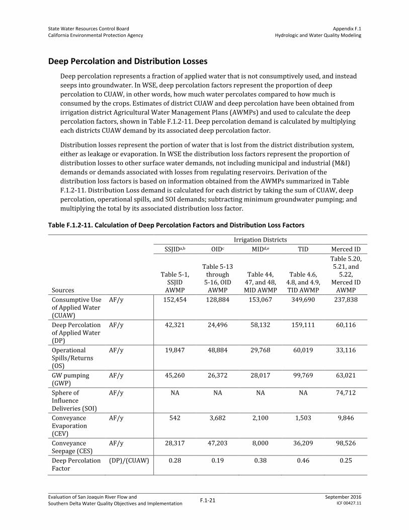
State Water Resources Control Board California Environmental Protection Agency
Appendix F.1 Hydrologic and Water Quality Modeling
Evaluation of San Joaquin River Flow and Southern Delta Water Quality Objectives and Implementation
F.1-21 September 2016
ICF 00427.11
Deep Percolation and Distribution Losses
Deep percolation represents a fraction of applied water that is not consumptively used, and instead
seeps into groundwater. In WSE, deep percolation factors represent the proportion of deep
percolation to CUAW, in other words, how much water percolates compared to how much is
consumed by the crops. Estimates of district CUAW and deep percolation have been obtained from
irrigation district Agricultural Water Management Plans (AWMPs) and used to calculate the deep
percolation factors, shown in Table F.1.2-11. Deep percolation demand is calculated by multiplying
each districts CUAW demand by its associated deep percolation factor.
Distribution losses represent the portion of water that is lost from the district distribution system,
either as leakage or evaporation. In WSE the distribution loss factors represent the proportion of
distribution losses to other surface water demands, not including municipal and industrial (M&I)
demands or demands associated with losses from regulating reservoirs. Derivation of the
distribution loss factors is based on information obtained from the AWMPs summarized in Table
F.1.2-11. Distribution Loss demand is calculated for each district by taking the sum of CUAW, deep
percolation, operational spills, and SOI demands; subtracting minimum groundwater pumping; and
multiplying the total by its associated distribution loss factor.
Table F.1.2-11. Calculation of Deep Percolation Factors and Distribution Loss Factors
Sources
Irrigation Districts
SSJIDa,b OIDc MIDd,e TID Merced ID
Table 5-1, SSJID
AWMP
Table 5-13 through
5-16, OID AWMP
Table 44, 47, and 48, MID AWMP
Table 4.6, 4.8, and 4.9, TID AWMP
Table 5.20, 5.21, and
5.22, Merced ID
AWMP
Consumptive Use of Applied Water (CUAW)
AF/y 152,454 128,884 153,067 349,690 237,838
Deep Percolation of Applied Water (DP)
AF/y 42,321 24,496 58,132 159,111 60,116
Operational Spills/Returns (OS)
AF/y 19,847 48,884 29,768 60,019 33,116
GW pumping (GWP)
AF/y 45,260 26,372 28,017 99,769 63,021
Sphere of Influence Deliveries (SOI)
AF/y NA NA NA NA 74,712
Conveyance Evaporation (CEV)
AF/y 542 3,682 2,100 1,503 9,846
Conveyance Seepage (CES)
AF/y 28,317 47,203 8,000 36,209 98,526
Deep Percolation Factor
(DP)/(CUAW) 0.28 0.19 0.38 0.46 0.25

State Water Resources Control Board California Environmental Protection Agency
Appendix F.1 Hydrologic and Water Quality Modeling
Evaluation of San Joaquin River Flow and Southern Delta Water Quality Objectives and Implementation
F.1-22 September 2016
ICF 00427.11
Sources
Irrigation Districts
SSJIDa,b OIDc MIDd,e TID Merced ID
Table 5-1, SSJID
AWMP
Table 5-13 through
5-16, OID AWMP
Table 44, 47, and 48, MID AWMP
Table 4.6, 4.8, and 4.9, TID AWMP
Table 5.20, 5.21, and
5.22, Merced ID
AWMP
Distribution Loss Factor
(CEV+CES)/ (CUAW+DP+OS+SOI-GWP)
0.17 0.29 0.05 0.08 0.32
Notes: a. South San Joaquin ID operational spill/returns are the sum of lateral spills (17,029 AF, Table 5-1), Lateral Seepage (8,165 AF, Table 5-1), and Tailwater (2,541 AF, Table 5-1). b. South San Joaquin ID conveyance seepage is the sum of main canal seepage (20,152 AF, Table 5-1) and lateral seepage (8,165 AF, Table 5-1). c. Oakdale ID GW pumping is the sum of district GW pumping (7,084 AF, Table 5-13) and private GW pumping (19,288 AF, Table 5-15). d. Modesto ID consumptive use of applied water was determined using the Crop ET (173,179 AF, Table 44) and subtracting annual effective precipitation (20,112 AF, Table 47). e. Modesto ID GW pumping is the sum of district GW pumping (20,057 AF, Table 47) and private GW pumping (7,960 AF, Table 48)
AF/y = acre feet per year
Operational Spills and Returns
Operational spills and returns represent water diverted by the districts that returns to the river.
Excess flow often is used to maintain constant pressure head in the distribution system and
maintain delivery. This water is eventually spilled or released from the distribution system and
returned to the river. Operational spills and returns are modeled as a constant timeseries of monthly
demands identical to CALSIM II return flow timeseries. In CALSIM II each district may have several
return flow timeseries, so for incorporation into the WSE total demand calculation, these return
flows have been aggregated into a single timeseries for each district. These flows return to the flow
node framework in the same location as in CALSIM (i.e., not aggregated).
Other Surface Water Demands
Other surface water demands accounted for in WSE include Woodward, Modesto, and Turlock
Reservoir Seepage; Modesto City M&I demands; and Merced ID Sphere of Influence (SOI) demands.
CALSIM II represents these demands as constant annual volumes distributed in the same monthly
patterns every year. After some analysis, it has been determined that CALSIM II estimates for these
annual demands can be refined to represent baseline conditions. Effort was made to acquire more
accurate and up-to-date estimates for these parameters, which are shown in Table F.1.2-12. On the
left of the table are shown the original CALSIM II estimates, and on the right are estimates derived
from more recent sources such as irrigation district AWMPs, information request response letters
from the irrigation districts, and the Merced Operations model released as part of Merced ID’s FERC
relicensing process (FERC 2015). In addition, another M&I demand was added for SSJID to represent
Degroot Water Treatment Plant (WTP) based on information in the SSJID AWMP (SSJID 2012). With
these new parameters, WSE diverges slightly from the CALSIM calibration and representation of
baseline; therefore, separate modes were created, one, CALSIM mode, to try and replicate CALSIM II

State Water Resources Control Board California Environmental Protection Agency
Appendix F.1 Hydrologic and Water Quality Modeling
Evaluation of San Joaquin River Flow and Southern Delta Water Quality Objectives and Implementation
F.1-23 September 2016
ICF 00427.11
operations using all the CALSIM II parameters and another, CEQA mode, to model the LSJR
alternatives with more up-to-date information, representing the most appropriate baseline
determined by SWRCB.
Woodward Reservoir, Modesto Reservoir, and Turlock Reservoir are regulating reservoirs used by
the districts to provide off stream storage for diversions and regulate irrigation water deliveries.
Woodward Res. serves South San Joaquin Irrigation District (SSJID), Modesto Res. serves Modesto
Irrigation District (MID), and Turlock Res. serves Turlock Irrigation District (TID). To keep these
reservoirs in operation, water losses to seepage must be replaced. These terms also include any
seepage losses from the upstream conveyance systems. In WSE these, annual demands are of the
same quantity and distributed in the same monthly pattern as in CALSIM.
The City of Modesto has an agreement with MID to purchase Tuolumne River water from the district
to reduce the city’s reliance on groundwater. In WSE, this annual demand is distributed in the same
monthly pattern as it is distributed in CALSIM. Operation of the Degroot WTP began in 2005, and it
serves the cities of Manteca, Lathrop, and Tracy with Stanislaus river water delivered from SSJID.
This demand was not included in CALSIM II because it came online after the model was constructed.
In WSE, this demand is represented as a constant annual volume distributed equally over all
months. In WSE, M&I surface water demands are assumed to be diverted directly from the district’s
regulating reservoir and do not pass through the district’s distribution system, so they are not
considered in the calculation of distribution losses shown above.
Table F.1.2-12. Other Annual Demands for Each Irrigation District
Parameters Irrigation District
WSE CALSIM Mode WSE CEQA Mode
Annual Total (TAF/y) Source
Annual Total (TAF/y) Source
Woodward Reservoir Losses SSJID 62 CALSIM 29.5 SSJID AWMP
Modesto Reservoir Losses MID 55 CALSIM 31.2 MID AWMP
Turlock Reservoir Losses TID 92 CALSIM 46.8 TID Info Request
Modesto M&I Demand MID 65 CALSIM 30.0 MID AWMP
Degroot WTP M&I Demand SSJID 15.7 SSJID AWMP 15.7 SSJID AWMP
Merced Sphere of Influence (SOI) Demandsa
Merced ID
81.4
CALSIM
68
Merced Operations
Model
Notes: a. Merced SOI demands include Merced National Wildlife Refuge (15 TAF/y, both modes), Stevinson (26.4 TAF/y CALSIM, 24 TAF/y CEQA), El Nido (40 TAF/y CALSIM, 13 TAF/y CEQA), and other SOI demand (0 TAF/y CALSIM, 16 TAF/y CEQA).
TAF/y = thousand acre-feet per year
Merced ID SOI demands occur outside of the district, but share the districts distribution system. The
SOI demands include the Stevinson Entitlement, required deliveries to Bear Creek in the Merced
National Wildlife Refuge (NWR) as part of the districts FERC license, deliveries to El Nido, and water
sales by Merced ID to other nearby entities (Merced ID 2013). Because these demands share the
district’s distribution system, they are included in calculations of distribution loss demand. El Nido
was actually incorporated into the district in 2005 (Merced ID 2013); however, CALSIM II
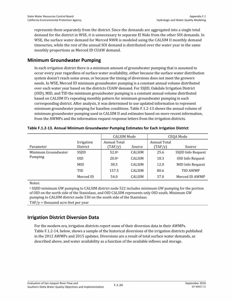
State Water Resources Control Board California Environmental Protection Agency
Appendix F.1 Hydrologic and Water Quality Modeling
Evaluation of San Joaquin River Flow and Southern Delta Water Quality Objectives and Implementation
F.1-24 September 2016
ICF 00427.11
represents them separately from the district. Since the demands are aggregated into a single total
demand for the district in WSE, it is unnecessary to separate El Nido from the other SOI demands. In
WSE, the surface water demand for Merced NWR is modeled using the CALSIM II monthly demand
timeseries, while the rest of the annual SOI demand is distributed over the water year in the same
monthly proportions as Merced ID CUAW demand.
Minimum Groundwater Pumping
In each irrigation district there is a minimum amount of groundwater pumping that is assumed to
occur every year regardless of surface water availability, either because the surface water distribution
system doesn’t reach some areas, or because the timing of diversions does not meet the growers
needs. In WSE, Merced ID minimum groundwater pumping is a constant annual volume distributed
over each water year based on the districts CUAW demand. For SSJID, Oakdale Irrigation District
(OID), MID, and TID the minimum groundwater pumping is a constant annual volume distributed
based on CALSIM II’s repeating monthly pattern for minimum groundwater pumping in each
corresponding district. After analysis, it was determined to use updated information to represent
minimum groundwater pumping for baseline conditions. Table F.1.2-13 shows the annual volume of
minimum groundwater pumping used in CALSIM II and estimates based on more recent information,
from the AWMPs and the information request response letters from the irrigation districts.
Table F.1.2-13. Annual Minimum Groundwater Pumping Estimates for Each Irrigation District
Parameter Irrigation District
CALSIM Mode CEQA Mode
Annual Total (TAF/y) Source
Annual Total (TAF/y) Source
Minimum Groundwater Pumping
SSJID 52.0a CALSIM 25.6 SSJID Info Request
OID 20.0a CALSIM 18.3 OID Info Request
MID 38.5 CALSIM 12.0 MID Info Request
TID 157.5 CALSIM 80.6 TID AWMP
Merced ID 54.0 CALSIM 37.0 Merced ID AWMP
Notes: a. SSJID minimum GW pumping to CALSIM district node 522 includes minimum GW pumping for the portion of OID on the north side of the Stanislaus, and OID CALSIM represents only OID south. Minimum GW pumping to CALSIM district node 530 on the south side of the Stanislaus.
TAF/y = thousand acre-feet per year
Irrigation District Diversion Data
For the modern era, irrigation districts report some of their diversion data in their AWMPs.
Table F.1.2-14, below, shows a sample of the historical diversions of the irrigation districts published
in the 2012 AWMPs and 2015 updates. Diversions are a result of total surface water demands, as
described above, and water availability as a function of the available inflows and storage.

State Water Resources Control Board California Environmental Protection Agency
Appendix F.1 Hydrologic and Water Quality Modeling
Evaluation of San Joaquin River Flow and Southern Delta Water Quality Objectives and Implementation
F.1-25 September 2016
ICF 00427.11
Table F.1.2-14. Sample of Irrigation District Diversion Data Reported in AWMPs
Water Year WY Type SSJID OID MID TIDa Merced ID
2000 AN 229,632 483,391
2001 D 217,940 465,222
2002 D 249,271 470,156
2003 BN 228,117 431,926
2004 D 262,500 463,744
2005 W 204,501 223,706
468,724
2006 W 222,390 225,614
484,759
2007 C 249,569 261,896 296,000 499,137 430,739
2008 C 252,483 244,606 288,000 441,466 312,072
2009 BN 244,059 234,424 267,300 466,063
2010 AN 223,202 217,143 264,633b 531,107
2011 W 219,289 218,147 315,912b 537,685
Average
233,579 232,219 286,369 495,092 445,637 a. In the 2012 AWMP, TID reports diversions measured below Turlock Reservoir, not from the river. b. Modesto ID in the 2015 update AWMP reports 2010 and 2011 diversion totals as 261,728 AF and 282,640 AF, respectively.
Sources:
SSJID AWMP 2015; OID AWMP 2012; MID AWMP 2012; TID AWMP 2012; Merced ID AWMP 2012
Comparison of Surface Water Demands
Under WSE-CALSIM mode, an adjustment factor was applied to each river’s CUAW demand to align
the resulting annual diversions to the magnitude and distribution of total annual diversions
calculated by SWRCB-CALSIM II. Similarly, under WSE-CEQA mode, a factor was applied to the
CUAW demand on each river so that the total annual diversions would be consistent with the
diversion levels represented in the Merced, Tuolumne, and Stanislaus operations models (MID 2015;
MID and TID 2013; SJTA 2012).3 Table F.1.2-15 contains the final adjustment factors applied to
CUAW demand for each irrigation district to determine the total surface water demand time series
from each river.
3 Stanislaus, Tuolumne, and Merced Operations Models may differ from CALSIM and WSE in their system representation of inflows, allocations, assumptions, and dynamics, but Operations Models diversions are t sufficiently representative of baseline irrigation district diversions (meeting full demands when possible, otherwise limited by water availability), as represented by the districts themselves. They are more up to date than available CALSIM CUAW representations. CALSIM CUAW is utilized within WSE, adjusted as described above, because the time series of CALSIM CUAW is essential to representing the inter-annual pattern of demand that varies as a function of weather conditions. Primarily, the most important aspect is characterization of maximum demand. Stanislaus Operations Model and CALSIM maximum demands are in excess of recent irrigation diversions, but are considered to account for some exercise of OID/SSJID entitlements under the 1988 Agreement that would take the form of water transfers or sales not considered in the model. Tuolumne maximum demands in the FERC Tuolumne Operations model are lower than either CALSIM or long-term historical diversions, but match more closely with recent AWMP reported diversions, so WSE-CEQA diversions have been adjusted downward accordingly. Merced ID maximum diversions in the Merced Operations Model are similar to CALSIM, but these levels of demand can be met less often in the CALSIM and WSE allocation schemes. The recent drought has illustrated that zero allocations do occur for Merced ID based on low available storage in New Exchequer Reservoir.
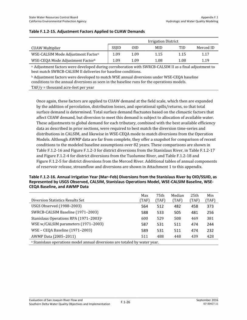
State Water Resources Control Board California Environmental Protection Agency
Appendix F.1 Hydrologic and Water Quality Modeling
Evaluation of San Joaquin River Flow and Southern Delta Water Quality Objectives and Implementation
F.1-26 September 2016
ICF 00427.11
Table F.1.2-15. Adjustment Factors Applied to CUAW Demands
CUAW Multiplier
Irrigation District
SSJID OID MID TID Merced ID
WSE-CALSIM Mode Adjustment Factora 1.09 1.09 1.15 1.15 1.17
WSE-CEQA Mode Adjustment Factorb 1.09 1.09 1.08 1.08 1.19
a. Adjustment factors were developed during corroboration with SWRCB-CALSIM II as a final adjustment to best match SWRCB-CALSIM II deliveries for baseline conditions. b. Adjustment factors were developed to match WSE annual diversions under WSE-CEQA baseline conditions to the annual diversions as seen in the baseline runs for the operations models.
TAF/y = thousand acre-feet per year
Once again, these factors are applied to CUAW demand at the field scale, which then are expanded
by the addition of percolation, distribution losses, and operational spills/returns, so that total
surface demand is determined. Total surface demand fluctuates based on the climactic factors that
affect CUAW demand, but diversion to meet this demand is subject to allocation of available water.
These adjustments to global demand for each tributary, combined with the best available efficiency
data as described in prior sections, were required to best match the diversion time-series and
distributions in CALSIM, and likewise in WSE-CEQA mode to match diversions from the Operation
Models. Although AWMP data are far from complete, they offer a snapshot for comparison of recent
conditions to the modeled baseline assumptions over 82 years. These comparisons are shown in
Table F.1.2-16 and Figure F.1.2-3 for district diversions from the Stanislaus River, in Table F.1.2-17
and Figure F.1.2-4 for district diversions from the Tuolumne River, and Table F.1.2-18 and
Figure F.1.2-5 for district diversions from the Merced River. Additional tables of annual components
of reservoir release, streamflow and diversions are shown in Attachment 1 to this appendix.
Table F.1.2-16. Annual Irrigation Year (Mar–Feb) Diversions from the Stanislaus River by OID/SSJID, as Represented by USGS Observed, CALSIM, Stanislaus Operations Model, WSE-CALSIM Baseline, WSE-CEQA Baseline, and AWMP Data
Diversion Statistics Results Set Max
(TAF) 75th
(TAF) Median (TAF)
25th (TAF)
Min (TAF)
USGS Observed (1988–2003) 564 512 482 458 373
SWRCB-CALSIM Baseline (1971–2003) 588 533 505 481 256
Stanislaus Operations RPA (1971–2003)a 600 529 508 469 381
WSE w/CALSIM parameters (1971–2003) 587 531 511 474 244
WSE – CEQA Baseline (1971–2003) 589 531 511 474 232
AWMP Data (2005–2011) 511 488 448 439 428 a Stanislaus operations model annual diversions are totaled by water year.

State Water Resources Control Board California Environmental Protection Agency
Appendix F.1 Hydrologic and Water Quality Modeling
Evaluation of San Joaquin River Flow and Southern Delta Water Quality Objectives and Implementation
F.1-27 September 2016
ICF 00427.11
0
100
200
300
400
500
600
700
Observed(1988 - 2003)
CALSIM(1971 - 2003)
Stan Ops(1971 - 2003)*
WSE - CALSIM(1971 - 2003)
WSE - CEQA(1971 - 2003)
AWMP Data(2005 - 2011)
An
nu
al D
ive
rsio
n (
TAF)
Figure F.1.2-3. Annual Irrigation Year (Mar–Feb) Diversions from the Stanislaus River by OID/SSJID, as
represented by USGS Observed, SWRCB-CALSIM, Stanislaus Operations Model (*Statistics are for
Annual Water Year Diverions), WSE-CALSIM Baseline, WSE-CEQA Baseline, and AWMP Data
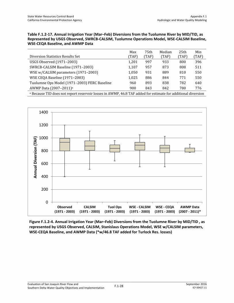
State Water Resources Control Board California Environmental Protection Agency
Appendix F.1 Hydrologic and Water Quality Modeling
Evaluation of San Joaquin River Flow and Southern Delta Water Quality Objectives and Implementation
F.1-28 September 2016
ICF 00427.11
Table F.1.2-17. Annual Irrigation Year (Mar–Feb) Diversions from the Tuolumne River by MID/TID, as Represented by USGS Observed, SWRCB-CALSIM, Tuolumne Operations Model, WSE-CALSIM Baseline, WSE-CEQA Baseline, and AWMP Data
Diversion Statistics Results Set Max
(TAF) 75th
(TAF) Median (TAF)
25th (TAF)
Min (TAF)
USGS Observed (1971–2003) 1,201 997 933 800 396
SWRCB-CALSIM Baseline (1971–2003) 1,107 957 873 808 511
WSE w/CALSIM parameters (1971–2003) 1,050 931 889 810 550
WSE CEQA Baseline (1971–2003) 1,025 886 844 771 550
Tuolumne Ops Model (1971–2003) FERC Baseline 960 893 838 782 640
AWMP Data (2007–2011)a 900 843 842 780 776 a Because TID does not report reservoir losses in AWMP, 46.8 TAF added for estimate for additional diversion
0
200
400
600
800
1000
1200
1400
Observed(1971 - 2003)
CALSIM(1971 - 2003)
Tuol Ops(1971 - 2003)
WSE - CALSIM(1971 - 2003)
WSE - CEQA(1971 - 2003)
AWMP Data(2007 - 2011)*
An
nu
al D
iver
sio
n (
TAF)
Figure F.1.2-4. Annual Irrigation Year (Mar–Feb) Diversions from the Tuolumne River by MID/TID , as represented by USGS Observed, CALSIM, Stanislaus Operations Model, WSE w/CALSIM parameters, WSE-CEQA Baseline, and AWMP Data (*w/46.8 TAF added for Turlock Res. losses)

State Water Resources Control Board California Environmental Protection Agency
Appendix F.1 Hydrologic and Water Quality Modeling
Evaluation of San Joaquin River Flow and Southern Delta Water Quality Objectives and Implementation
F.1-29 September 2016
ICF 00427.11
Table F.1.2-18. Annual Irrigation Year (Mar-Feb) Diversions from the Merced River by Merced ID, as Represented by Observed, CALSIM, Merced Operations Model, WSE w/CALSIM parameters, WSE-CEQA Baseline, and AWMP Data
Diversion Statistics Results Set Max
(TAF) 75th
(TAF) Median (TAF)
25th (TAF)
Min (TAF)
SWRCB CALSIM Baseline D561 (1971–2003) 528 493 462 432 42
WSE w/CALSIM parameters D561 (1971–2003) 542 501 456 414 14
WSE CEQA Baseline D561 (1971–2003) 542 503 467 424 3
Merced Ops Model/Observed (1970–2003) 535 498 477 456 60
AWMP Data (2000–2008) 485 470 465 432 312
0
100
200
300
400
500
600
CALSIM(1971 - 2003)
Merc Ops /Observed
(1970 - 2003)
WSE - Calsim(1971 - 2003)
WSE - CEQA(1971 - 2003)
AWMP Data(2000-2008)
An
nu
al D
iver
sio
n (
TAF)
Figure F.1.2-5. Annual Irrigation Year (Mar–Feb) Diversions from the Merced River by Merced ID, as
Represented by SWRCB-CALSIM Baseline, Merced Operations Model, WSE-CALSIM Baseline, WSE-
CEQA Baseline, and AWMP Data

State Water Resources Control Board California Environmental Protection Agency
Appendix F.1 Hydrologic and Water Quality Modeling
Evaluation of San Joaquin River Flow and Southern Delta Water Quality Objectives and Implementation
F.1-30 September 2016
ICF 00427.11
CVP Contractor Demands
The CVP contractors, Stockton East Water District (SEWD) and Central San Joaquin Water
Conservation District (CSJWCD) are treated differently compared to the other districts. Their
demands are represented as a constant annual volume of 155 thousand acre-feet per year (TAF/y)
(with 80 TAF/y for CSJWCD and 75 TAF/y for SEWD) based on information from USBR
(USBR 2013a, 2013b). This demand is distributed over the year in a monthly pattern, as shown in
Table F.1.2-19.
Table F.1.2-19. CVP Contractor Monthly Diversion Schedule
Month
SEWD/CSJWCD
Monthly Demand Pattern (% of Annual)
Modeled Demand (TAF)
January 3% 5
February 3% 5
March 4% 6
April 4% 6
May 11% 17
June 18% 27
July 20% 31
August 15% 24
September 9% 13
October 5% 8
November 4% 7
December 4% 6
Total 100% 155
Minor, Riparian, and Cowell Agreement Diversion Demands
Finally, minor and riparian demands represent diverters with riparian rights or smaller diversions
along each tributary. In WSE, these demands are modeled using the monthly timeseries of
diversions taken from CALSIM II (D528 and D545) and are kept separate from the district demands.
The CAD demands are also treated as minor and riparian demands in WSE. However, the SWRCB-
CALSIM II timeseries of CAD diversions (D528) does not fully divert the Cowell Agreement Flow
described in Table F.1.2-7. Under CEQA mode in WSE the monthly CAD demands were increased so
that they would equal that month’s Cowell Agreement Flow Release.
F.1.2.5 Calculation of Available Water for Diversion
As a part of the modeling analysis, it has been necessary to utilize certain reservoir constraints and
parameters that determine allocation of available water for diversions, both in baseline and
alternatives scenarios. These parameters are central to the model’s determination of when there is
available water to meet full irrigation demands and, at other times, when there is not adequate
water supply from inflow and reservoir storage, which, in turn, requires diminished allocations of
water to diversions while preserving a reserve of storage supply for future years.

State Water Resources Control Board California Environmental Protection Agency
Appendix F.1 Hydrologic and Water Quality Modeling
Evaluation of San Joaquin River Flow and Southern Delta Water Quality Objectives and Implementation
F.1-31 September 2016
ICF 00427.11
The analysis contained in this SED provides LSJR alternatives that represent examples of system
operation to determine the significance of impacts, pursuant to CEQA. Selection of appropriate
parameters has first been made to represent baseline conditions most closely in terms of diversion
allocations and reservoir operations, similar to those in the CALSIM baseline scenario. Under
additional streamflow requirements of the LSJR alternatives, changes in water availability require
adjustment of parameters to ensure feasibility for the 82-year simulation so that the reservoirs are
not drained entirely in the worst droughts of record. In addition, carryover storage guidelines have
been increased for New Melones Reservoir and New Exchequer Reservoir to minimize impacts on
instream temperature that would be caused by lower reservoir levels and a limited coldwater pool.
These operational constraints, as components of modeling simulations, do not by themselves
comprise a plan of implementation or otherwise carry the weight of regulatory requirements.
Rather, they are included as elements of the modeling simulation to evaluate the feasibility of the
LSJR alternatives. An implementation plan developed in a future proceeding would need to identify
and evaluate supply, storage, and temperature conditions and appropriate operational objectives, to
best protect beneficial uses and avoid adverse effects where feasible.
In WSE, the following operational parameters are used to govern reservoir operations and
determination4 of the available water for diversion and use:
Maximum Storage Levels (Flood Curves): The maximum level allowable in the reservoir is set
equal to the CALSIM flood control levels in New Melones and New Don Pedro Reservoirs
(including conditional storage, when applicable) and Lake McClure. The model assumes
projected filling above these levels will be evacuated within that month to maintain at or below
these maximum operating levels. These flood curves are based on USACE requirements, but with
some differences (USBR 2005).
Minimum End-of-September Storage: A minimum end-of-September storage guideline was
developed by iteration in order to determine levels protective of coldwater pool and river
temperatures in the summer and fall. Projected end-of-September storage for a given year is
reduced by this value to determine the amount of storage supply available for diversion for that
year.
Minimum Diversion Level (Minimum End-of-September Relaxation): Diversions can override
the end-of September storage guideline and draw additional water from storage in the event the
available surface water for diversion is less than a specified minimum level. This in effect is a
relaxation in certain years to the end-of-September storage guideline. The minimum level
constraint was set after trial and error to ensure there were no significant temperature impacts.
Maximum Allowable Draw from Storage: The model constrains the percentage of the available
storage (after holding back for minimum end-of-September storage) that is available for
diversion over the irrigation season. This limits the amount of storage that can be withdrawn to
reduce potential effects on river temperatures by protecting carryover storage and the
4 Determination of available water to supply demand is a modeling necessity to represent baseline conditions and operational envelopes for LSJR alternatives; however, these parameters, including “Maximum Allowable Draw from Storage,” do not represent regulatory requirements of how the reservoir storage and use system must be operated—rather, alternatives are examples of system operation that illustrate most likely water availability as a function of additional constraints of instream flow requirements. To some extent, carryover storage guidelines have been increased over baseline to reduce indirect temperature effects that would otherwise occur because of lower storage levels. Implementation most likely will require further optimization of these parameters with balanced consideration of desired temperatures and tradeoffs with other resource values.

State Water Resources Control Board California Environmental Protection Agency
Appendix F.1 Hydrologic and Water Quality Modeling
Evaluation of San Joaquin River Flow and Southern Delta Water Quality Objectives and Implementation
F.1-32 September 2016
ICF 00427.11
coldwater pool in the reservoirs leading into a drought sequence. Baseline “allowable draw” was
determined empirically to match CALSIM patterns of allocations, similar to how a “delivery
versus carryover risk curve” might be used.
End-of-Drought Storage Refill Requirement (only needed in alternatives with 40+ percent of
unimpaired flow, not in baseline): When reservoir levels are very low (typically after a drought
sequence), the model limits the amount of inflow that can be allocated for diversion in a
subsequent wet year(s). By reducing the amount of inflow that can be diverted in such years,
reservoirs and associated coldwater pools recover more quickly after a drought. Without such a
requirement, reservoirs otherwise would remain lower for longer after a drought, causing
associated temperature impacts.
Calculation of available water proceeds as follows:
After the instream flow and other environmental release requirements are satisfied, the available
water for diversions is calculated for each year’s growing season. Available water for diversion is the
amount of projected inflow plus carryover storage adjusted downward by the amount of required
flow releases, the first estimate of reservoir evaporation, and the end-of-September storage
guidelines.
Equation F.1-2 shows the calculation to determine available water for diversion, Wavail,GS:
𝑊𝑎𝑣𝑎𝑖𝑙 ,𝐺𝑆 = 𝐾𝑆𝑡𝑜𝑟 ∗ 𝑆𝑎 − 𝐸𝑂𝑆𝑟𝑒𝑞
𝐴𝑣𝑎𝑖𝑙𝑎𝑏𝑙𝑒 𝑆𝑡𝑜𝑟𝑎𝑔𝑒
+ (𝑄𝐼𝑁𝐹𝑛 − 𝐸𝑅𝑛 − 𝐸𝑉𝑛)
𝑏
𝑛=𝑎+1
𝐴𝑣𝑎𝑖𝑙𝑎𝑏𝑙𝑒 𝐼𝑛𝑓𝑙𝑜𝑤
(Eqn. F.1-2)
Where:
KStor is the percentage of the available storage at the tributary’s major reservoir that would be
available for diversion over the growing season. In general, this value limits the amount of
storage that can be withdrawn, reducing potential impacts on river temperatures by protecting
the reservoir’s coldwater pool.
Sa is the ending storage at the tributary’s major reservoir for month a. Month a is selected by the
user and represents the last month prior to the start of the growing season; a = 2 (February) for
the baseline and alternative simulations.
EOSreq is the minimum end-of-September carryover storage guideline at the tributary’s major
reservoir that would protect coldwater pool and river temperatures in the summer and fall.
QINF is the forecast CALSIM II inflow to the tributary’s major reservoir over the growing season,
from month a+1 to month b. Month b is also selected by the user and represents the final month of
the growing season; b = 9 (September) for the baseline and alternative simulations. The inflow
time series for each reservoir was developed by DWR and USBR outside of CALSIM II as an input
to CALSIM II. The New Melones Reservoir inflows, developed by USBR, are a combination of
planning study inflows and actual recorded inflows for recent years; the New Don Pedro Reservoir
inflows, provided by the City and County of San Francisco (CCSF), are a result of a long-term
simulation of current project operations for the period prior to 1996 and actual computed inflow
since 1996. The Lake McClure inflows were estimated using the Lake McClure outflows adjusted
for change in storage and evaporation in Lake McClure (USBR 2005).

State Water Resources Control Board California Environmental Protection Agency
Appendix F.1 Hydrologic and Water Quality Modeling
Evaluation of San Joaquin River Flow and Southern Delta Water Quality Objectives and Implementation
F.1-33 September 2016
ICF 00427.11
ER is the sum of monthly reservoir releases over the growing season to meet all instream flow
and environmental requirements for the tributary. This includes reservoir releases to meet the
depletions along the river, the unimpaired flow requirement, the tributary minimum flows, the
flow shifting requirements, the CAD flow requirement on the Merced, VAMP, D1641, and
Vernalis minimum flow and EC.
EV is forecast total evaporation from the tributary’s major reservoir over the growing season. For
this available water calculation, the monthly evaporation timeseries is taken directly from CALSIM
values.5
Figure F.1.2-6. Illustration of Available Storage Calculation for the Example Year 1991
5 CALSIM seasonal evaporation quantities (based on CALSIM baseline reservoir volumes and rates) are sufficient for a first-order estimate of available water for diversion. After the allocation of available water is performed, the final water balance is calculated, with the monthly evaporation calculation based on the actual reservoir volume and surface area, using the CALSIM rates. This approach was a method to avoid circular references in Excel.

State Water Resources Control Board California Environmental Protection Agency
Appendix F.1 Hydrologic and Water Quality Modeling
Evaluation of San Joaquin River Flow and Southern Delta Water Quality Objectives and Implementation
F.1-34 September 2016
ICF 00427.11
Table F.1.2-20. Baseline End-of-September Storage Guidelines, Maximum Draw from Storage, and Minimum Diversion Variables for the Eastside Tributaries
Variable Stanislaus River Tuolumne River Merced River
End-of-September Storage Guideline (TAF) 85 800 115
Maximum Draw from Storage (% of available storage)
80% 65% 80%
Minimum Diversion (TAF) 0 550 0
Evaporation
For the three major reservoirs, evaporation is a function of the evaporation rate and the surface area
of the reservoirs. CALSIM rates are used for each month of the simulation, and the area of each
reservoir is recalculated by WSE using a volume/area relationship. Note that in order to prevent
circular references, the available water allocation is made using CALSIM estimates of evaporation
(based on SWRCB-CALSIM baseline, the evaporation from reservoirs based on levels in that
scenario), while the final water balance is performed with evaporation recalculated more precisely
by WSE, based on the volume-area relationships contained in Tables F.1.2-21a, F.1.2-b, and F.1.2-c.
Table F.1.2-21a. Area/Volume Relationship for New Melones Reservoir for Calculating Evaporation
Elevation (ft. MSL) Storage (TAF) Area (acres)
500.00 0.98 2
700.00 53.90 1,217
760.00 160.55 2,374
808.00 299.52 3,446
920.00 846.52 6,485
992.00 1,398.83 8,901
1,049.50 1,969.50 10,962
1,088.00 2,419.52 12,442
1,100.00 2,571.83 12,949
1,123.40 2,871.00 14,011
Table F.1.2-21b. Area/Volume Relationship for New Don Pedro Reservoir for Calculating Evaporation
Elevation (ft. MSL) Storage (TAF) Area (acres)
300.00 2.00 2
524.00 100.00 1,752
628.00 400.00 4,116
683.00 700.00 5,983
725.00 1,000.00 7,675
760.00 1,300.00 9,270
791.00 1,600.00 10,800
820.00 1,900.00 12,283
847.00 2,200.00 13,732
872.00 2,500.00 15,151

State Water Resources Control Board California Environmental Protection Agency
Appendix F.1 Hydrologic and Water Quality Modeling
Evaluation of San Joaquin River Flow and Southern Delta Water Quality Objectives and Implementation
F.1-35 September 2016
ICF 00427.11
Table F.1.2-21c. Area/Volume Relationship for New Exchequer Reservoir for Calculating Evaporation
Elevation (ft. MSL) Storage (TAF) Area (acres)
400.00 2.00 2
618.00 100.00 1,368
674.00 200.00 2,156
713.00 300.00 2,852
758.00 450.00 3,813
793.00 600.00 4,718
823.00 750.00 5,589
848.00 900.00 6,434
871.00 1,050.00 7,261
891.00 1,200.00 8,073
Table F.1.2-22. Annual Average Evaporation for New Melones, New Don Pedro, and New Exchequer Reservoirs for Baseline and LSJR Alternatives
Scenario Parameter New Melones New Don Pedro New Exchequer
ALL Avg. annual inflow (TAF) 1,087 1,586 965
BASELINE Avg. annual evap (TAF) 50 61 21
20%UF Avg. annual evap (TAF) 54 61 22
30%UF Avg. annual evap (TAF) 53 60 22
40%UF Avg. annual evap (TAF) 52 58 21
50%UF Avg. annual evap (TAF) 50 57 21
60%UF Avg. annual evap (TAF) 49 56 20
WSE Model Operational Parameters for the LSJR Alternatives
After a baseline WSE model was developed, it was modified to estimate the resulting flows,
diversions, and reservoir operations of the LSJR alternatives by adjusting the parameters in
Tables F.1.2-23a, F.1.2-23b, and F.1.2-23c to incorporate the alternative flow requirements. The
following sets of inputs were used in the WSE model for the alternatives and intermediate
simulations, ranging from 20 percent of unimpaired flow to 60 percent of unimpaired flow.

State Water Resources Control Board California Environmental Protection Agency
Appendix F.1 Hydrologic and Water Quality Modeling
Evaluation of San Joaquin River Flow and Southern Delta Water Quality Objectives and Implementation
F.1-36 September 2016
ICF 00427.11
Table F.1.2-23a. Minimum Diversion, Minimum September Carryover Guideline, Maximum Draw from Storage, and Flow Shifting for the Stanislaus River
Baseline
20% Unimpaired
Flow
30% Unimpaired
Flow
40% Unimpaired
Flow
50% Unimpaired
Flow
60% Unimpaired
Flow
Minimum District Diversion (TAF, % of District Max)
0 TAF 210 TAF (35%)
210 TAF (35%)
210 TAF (35%)
180 TAF (30%)
180 TAF (30%)
Minimum September Carryover Guideline (TAF)
85 700 700 700 700 700
Maximum Storage Draw (% of Mar 1 minus Sep guideline)
80% 80% 70% 50% 45% 35%
Flow Shifting to Falla NA None None Yes Yes Yes
End-of-Drought Storage Refill
NA 100% 100% 70% 50% 50%
Vernalis Minimumb Feb–Jun (cfs)
D-1641/ VAMP
1,000 1,000 1,000 1,000 1,000
TAF = thousand acre feet
cfs = cubic feet per second
a In the alternatives, the shifting of a portion of unimpaired flow requirement was completed during wet years, designed to allow only a percentage of diversions in the qualifying years (if storage was within 10% of the guideline September storage and inflow was projected to be higher than average). b For unimpaired flow alternatives, the Stanislaus River is assumed to provide 29 percent of additional releases necessary to meet the Vernalis minimum flow requirement based on its long-term fraction of unimpaired flow among the three eastside tributaries.

State Water Resources Control Board California Environmental Protection Agency
Appendix F.1 Hydrologic and Water Quality Modeling
Evaluation of San Joaquin River Flow and Southern Delta Water Quality Objectives and Implementation
F.1-37 September 2016
ICF 00427.11
Table F.1.2-23b. Minimum Diversion, Minimum September Carryover Guideline, Maximum Draw from Storage, and Adaptive Implementation for the Tuolumne River
Baseline
20% Unimpaired
Flow
30% Unimpaired
Flow
40% Unimpaire
d Flow
50% Unimpaired
Flow
60% Unimpaired
Flow
Minimum District Diversion (TAF, % of District Max)
550 TAF (50%)
363 TAF (33%)
363 TAF (33%)
363 TAF (33%)
275 TAF (20%)
275 TAF (20%)
Minimum September Carryover Guideline (TAF)
800 800 800 800 800 800
Maximum Storage Draw (% of Mar 1 minus Sep guideline)
65% 60% 55% 50% 45% 35%
Flow Shifting to Falla NA None None Yes Yes Yes
Drought End Storage Refill
NA 100% 100% 70% 50% 50%
Vernalis Minimumb Feb–Jun (cfs)
D-1641/ VAMP
1,000 1,000 1,000 1,000 1,000
TAF = thousand acre feet; cfs = cubic feet per second
a In the alternatives, the shifting of a portion of unimpaired flow requirement was completed during wet years, designed to allow only a percentage of diversions in the qualifying years (if storage was within 10% of the guideline September storage and inflow was projected to be higher than average). b For unimpaired flow alternatives, the Tuolumne River is assumed to provide 47 percent of additional releases necessary to meet the Vernalis minimum flow requirement based on its long-term fraction of unimpaired flow among the three eastside tributaries.
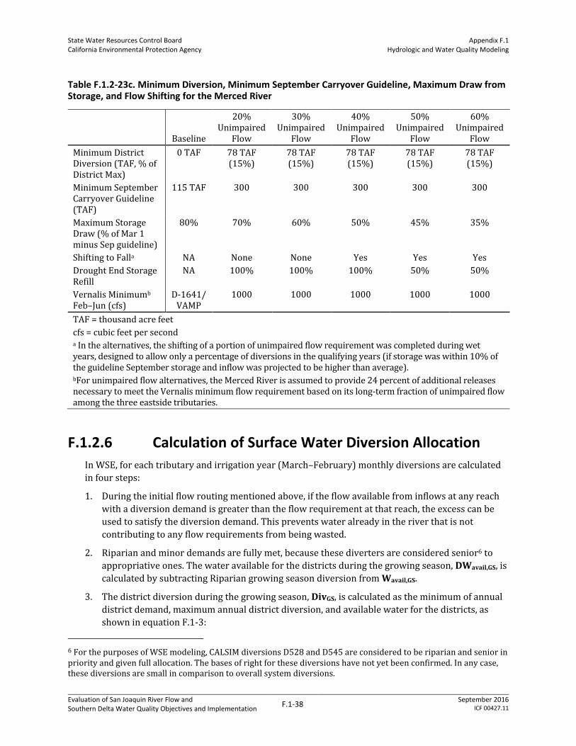
State Water Resources Control Board California Environmental Protection Agency
Appendix F.1 Hydrologic and Water Quality Modeling
Evaluation of San Joaquin River Flow and Southern Delta Water Quality Objectives and Implementation
F.1-38 September 2016
ICF 00427.11
Table F.1.2-23c. Minimum Diversion, Minimum September Carryover Guideline, Maximum Draw from Storage, and Flow Shifting for the Merced River
Baseline
20% Unimpaired
Flow
30% Unimpaired
Flow
40% Unimpaired
Flow
50% Unimpaired
Flow
60% Unimpaired
Flow
Minimum District Diversion (TAF, % of District Max)
0 TAF 78 TAF (15%)
78 TAF (15%)
78 TAF (15%)
78 TAF (15%)
78 TAF (15%)
Minimum September Carryover Guideline (TAF)
115 TAF 300 300 300 300 300
Maximum Storage Draw (% of Mar 1 minus Sep guideline)
80% 70% 60% 50% 45% 35%
Shifting to Falla NA None None Yes Yes Yes
Drought End Storage Refill
NA 100% 100% 100% 50% 50%
Vernalis Minimumb Feb–Jun (cfs)
D-1641/ VAMP
1000 1000 1000 1000 1000
TAF = thousand acre feet
cfs = cubic feet per second
a In the alternatives, the shifting of a portion of unimpaired flow requirement was completed during wet years, designed to allow only a percentage of diversions in the qualifying years (if storage was within 10% of the guideline September storage and inflow was projected to be higher than average). bFor unimpaired flow alternatives, the Merced River is assumed to provide 24 percent of additional releases necessary to meet the Vernalis minimum flow requirement based on its long-term fraction of unimpaired flow among the three eastside tributaries.
F.1.2.6 Calculation of Surface Water Diversion Allocation
In WSE, for each tributary and irrigation year (March–February) monthly diversions are calculated
in four steps:
1. During the initial flow routing mentioned above, if the flow available from inflows at any reach
with a diversion demand is greater than the flow requirement at that reach, the excess can be
used to satisfy the diversion demand. This prevents water already in the river that is not
contributing to any flow requirements from being wasted.
2. Riparian and minor demands are fully met, because these diverters are considered senior6 to
appropriative ones. The water available for the districts during the growing season, DWavail,GS, is
calculated by subtracting Riparian growing season diversion from Wavail,GS.
3. The district diversion during the growing season, DivGS, is calculated as the minimum of annual
district demand, maximum annual district diversion, and available water for the districts, as
shown in equation F.1-3:
6 For the purposes of WSE modeling, CALSIM diversions D528 and D545 are considered to be riparian and senior in priority and given full allocation. The bases of right for these diversions have not yet been confirmed. In any case, these diversions are small in comparison to overall system diversions.
State Water Resources Control Board California Environmental Protection Agency
Appendix F.1 Hydrologic and Water Quality Modeling
Evaluation of San Joaquin River Flow and Southern Delta Water Quality Objectives and Implementation
F.1-39 September 2016
ICF 00427.11
𝐷𝑖𝑣𝐺𝑆 = 𝑀𝑖𝑛 𝐷𝑚𝑥𝐺𝑆 , 𝐷𝑊𝑎𝑣𝑎𝑖𝑙 ,𝐺𝑆 , 𝐷𝑒𝑚𝐺𝑆 (Eqn. F.1-3)
Where:
DmxGS is the maximum allowable diversion over the growing season. For the Stanislaus the
annual maximum district diversion is distributed over the irrigation year based on the monthly
demands and then summed over the growing season. For the Tuolumne and Merced the annual
maximum district diversion was distributed monthly based on a repeating yearly pattern based
on typical monthly fractions in CALSIM over the growing season.
DemGS is the total growing season diversion demand. In general, demand is the limiting volume
during wet years, while available surface water is the limiting factor during dryer years.
On the Stanislaus there is an additional constraint to represent the growing season allowable
diversion under the 1988 Agreement, D1988. This agreement stipulates that SSJID and OID will
receive the first 600 TAF/y of inflow to New Melones or if the inflow is less than 600 TAF/y they
will receive the Inflow plus 1/3 x (600 minus inflow) (SSJID 2012). In WSE this annual total is
distributed over the irrigation year based on the monthly demands and then summed over the
growing season to determine D1988.
4. Finally, the total growing season diversion is distributed monthly to determine Divt, the
diversion in month t. It is assumed that the same proportion of demand met in the growing
season as a whole will be met in all months over the irrigation year. Equation F.1-4A shows the
calculation:
𝐷𝑖𝑣𝑡 = 𝐷𝑖𝑣𝐺𝑆 𝐷𝑒𝑚𝐺𝑆 𝑑𝑒𝑙𝑖𝑣𝑒𝑟𝑦 𝑝𝑟𝑜𝑝𝑜𝑟𝑡𝑖𝑜𝑛
∗ 𝐷𝑒𝑚𝑡 ∗ 𝐾𝑅𝑒𝑓𝑖𝑙𝑙 (Eqn. F.1-4A)
Where:
Demt is the district demand in month t.
KRefill is a reservoir refill user specified parameter between 0 and 1 that reduces diversion in an
effort to help refill the major reservoirs at the end of a drought. This parameter is activated if:
1) storage in the major reservoir at the end of the previous October was less than EOSreq plus
10 percent and 2) inflow to the major reservoir over the growing season will be greater than an
inflow trigger set by the user. This diversion cut will continue over the entire irrigation year
(March–February) unless the reservoir reaches the flood curve at which point the cut will end
for the rest of the year. However, if the calculated growing season diversion is less than the user
defined minimum annual diversion, monthly diversion will be determined using Eqn. F.1-4B:
𝐷𝑖𝑣𝑡 = 𝐷𝑚𝑛% ∗ 𝐷𝑚𝑥𝐼𝑌
𝑚𝑖𝑛 𝑎𝑛𝑛𝑢𝑎𝑙 𝑑𝑖𝑣𝑒𝑟𝑠𝑖𝑜𝑛
∗ 𝐷𝑒𝑚𝑡
𝐷𝑒𝑚𝐼𝑌
(Eqn. F.1-4B)
Where:
Dmn% is the minimum annual district diversion as a percent of maximum annual diversion.
This variable allows the diversion to override the end-of September storage guideline and draw
additional water from storage in the event the available surface water for diversion is less than
the minimum diversion level. Because this allows additional diversion, this variable could also
be considered a relaxation in some years to the end-of-September storage guideline. The

State Water Resources Control Board California Environmental Protection Agency
Appendix F.1 Hydrologic and Water Quality Modeling
Evaluation of San Joaquin River Flow and Southern Delta Water Quality Objectives and Implementation
F.1-40 September 2016
ICF 00427.11
minimum diversion rates were set for the baseline such that resulting diversion and storage
were similar to the results of CALSIM. As the unimpaired flow requirement increased, the
minimum diversion level was lowered to help balance the reservoir, reduce potential
temperature impacts, and ultimately maximize diversions.
DmxIY is the maximum annual district diversion over the irrigation year. The maximum district
diversion on each tributary is 600 TAF/y for the Stanislaus River, 1,100 TAF/y for the Tuolumne
River, and 542 TAF/y for the Merced River. These values did not change among simulations and
were held constant for each year.
DemIY is the total district demand over the irrigation year.
CVP Contractor Diversion
On the Stanislaus, diversion to the CVP contractors (SEWD and CSJWCD) is calculated differently
than for the other irrigation districts. The contractors receive diversion only after the senior district
has received its allocation of water based on the above calculations. The water available to the
contractors during the growing season would be DWavail,GS, minus any diversion to the senior
districts. Growing season water allocation to the contractors, CDivGS, is shown in equation F.1-5,
which is then distributed monthly, CDivt, in equation F.1-6:
𝐶𝐷𝑖𝑣𝐺𝑆 = 𝑀𝑖𝑛 𝐷𝑊𝑎𝑣𝑎𝑖𝑙 ,𝐺𝑆 − 𝐷𝑖𝑣𝐺𝑆 , 𝐶𝐷𝑒𝑚𝐺𝑆 (Eqn. F.1-5)
𝐶𝐷𝑖𝑣𝑡 = 𝑀𝑖𝑛 𝐶𝐾𝑐𝑢𝑡 ,
𝐶𝐷𝑖𝑣𝐺𝑆 ∗ 𝐾𝑅𝑒𝑓𝑖𝑙𝑙
𝐶𝐷𝑒𝑚𝐺𝑆 ∗ 𝐶𝐷𝑒𝑚𝑡
(Eqn. F.1-6)
Where:
CDemGS and CDemt are the total contractor water demand on the Stanislaus River over the
growing season and in month t, respectively.
CKcut is a user defined allocation factor based on the NMI (Table F.1.2-1 in the prior section).
This factor supersedes the calculated allocation based on water availability and demand unless
the calculated allocation is smaller.
F.1.2.7 Calculation of River and Reservoir Water Balance
Once the annual diversion is calculated, WSE begins a final flow routing through the rivers to
Vernalis including deliveries from the reservoirs to diversions. Because there are requirements at
Vernalis that depend on the flows from the tributaries, the model conducts multiple routing cycles to
determine the required release from the three major reservoirs. The first cycle determines the flow
that would occur at Vernalis assuming there were no requirements at Vernalis and no flood releases.
During the first cycle the resulting Vernalis flow is checked against the minimum flow requirement
at Vernalis and additional flow requirements are distributed among the tributaries if needed, as
described earlier under Calculations of Flow Targets. The second cycle determines the resulting flow
at Vernalis while including the Vernalis minimum flow requirement, VAMP requirements, and flood
control flows from the Merced and Tuolumne. During the Second cycle Vernalis flow is checked
against D1641 and then salinity requirements. If either D1641 or Vernalis Salinity is not met, any
additional flow needed is taken from the Stanislaus River. The final cycle re-calculates the tributary
and SJR flows through to Vernalis, including all required releases, diversions, and flood spills. The
equations below describe the reservoir and river flow calculations.

State Water Resources Control Board California Environmental Protection Agency
Appendix F.1 Hydrologic and Water Quality Modeling
Evaluation of San Joaquin River Flow and Southern Delta Water Quality Objectives and Implementation
F.1-41 September 2016
ICF 00427.11
Required Reservoir Releases
The required reservoir release needed to satisfy the target flows and diversions is determined
monthly on each eastside tributary as the sum of flow requirement, diversion, and flood control
release:
𝑅𝑡 = 𝐸𝑅𝑡 + 𝐷𝑖𝑣𝑡 + 𝐶𝐷𝑖𝑣𝑡 + 𝑅𝑖𝑝𝐷𝑡 + 𝐹𝑡 (Eqn. F.1-7)
Where:
ERt is the environmental flow release.
Divt is the irrigation district diversion, Cdivt is the CVP contractor diversion (only on the
Stanislaus), and RipDt is the riparian diversion (does not includes CAD diversions on the Merced
as those are accounted for in ERt).
Ft is the additional reservoir spill release required to stay below flood stage in New Melones and
New Don Pedro Reservoirs (as defined by the CALSIM flood storage curves in Table F.1.2-24) and
the discretionary hydropower operations level in Lake McClure. Spills are only necessary in months
when storage would otherwise exceed flood control limits.
Table F.1.2-24. CALSIM End-of-Month Flood Control Storage Limitations Applied to New Melones Reservoir, New Don Pedro Reservoir, and Lake McClure in the WSE Model
New Melonesa New Don Pedrob Lake McClurec
Calendar Month (TAF) (TAF) (TAF)
1 1,970 ---b 674.6
2 1,970 ---b 674.6
3 2,030 ---b 735
4 2,220 ---b 845
5 2,420 ---b 970
6 2,420 ---b 1,024
7 2,300 ---b 910
8 2,130 ---b 770
9 2,000 ---b 700
10 1,970 ---b 674.6
11 1,970 ---b 674.6
12 1,970 ---b 674.6
Notes: a.. Maximum storage volume (to spillway) in New Melones Reservoir is 2,420 TAF. b. “New Don Pedro Reservoir flood control constraints (reserved storage) are included in CALSIM II as a time series. The time series reflects end-of-month rain-flood reservation space and conditional reservation space during the snowmelt season per COE requirements” (USBR 2005). This 82-year monthly CALSIM time series is referenced by the WSE model for each month. Maximum storage in New Don Pedro Reservoir is 2,030 TAF. c. Maximum storage volume in Lake McClure is 1,024 TAF.

State Water Resources Control Board California Environmental Protection Agency
Appendix F.1 Hydrologic and Water Quality Modeling
Evaluation of San Joaquin River Flow and Southern Delta Water Quality Objectives and Implementation
F.1-42 September 2016
ICF 00427.11
Reservoir Storage Levels
Storage levels behind the major dams are initially set the same as CALSIM II levels at the end of
September, 1921 (951TAF in New Melones, 1,313 TAF in New Don Pedro, and 469 TAF in Lake
McClure). As with CALSIM II, the maximum level allowable in the reservoir is set equal to the flood
control levels in New Melones and New Don Pedro Reservoirs (including conditional storage, when
applicable) and Lake McClure, (Table F.1.2-24). The model assumes projected filling above these
levels will be evacuated within that month to maintain at or below these maximum operating levels.
The reservoir storage at the end of each subsequent month, St, is calculated with a water balance
equation on each tributary using:
St = St-1 +QINFt -Rt -EVt (Eqn. F.1-8)
Where:
St-1 is the ending storage of the previous month.
QINFt is the CALSIM II inflow to each major reservoir described above in Equation F.1-2; and
EVt is the evaporation from the major reservoir at time t. WSE evaporation is calculated using
the CALSIM II evaporation rates multiplied by the reservoir surface area at time t.
River Flows
The resulting flow achieved by the WSE model at the confluence of each of the three eastside
tributaries with the SJR is determined as follows:
𝑄𝑡 = 𝑅𝑡 − 𝐷𝑖𝑣𝑡 − 𝐶𝐷𝑖𝑣𝑡 − 𝑅𝑖𝑝𝐷𝑡 + 𝑄𝐴𝐶𝑡 (Eqn. F.1-9)
The flow resulting at Vernalis, QVt, is calculated as follows:
𝑄𝑉𝑡 = 𝑄𝑁𝑡 + 𝑄𝑡 3 𝑡𝑟𝑖𝑏𝑢𝑡𝑎𝑟𝑖𝑒𝑠 − 𝐷𝑣𝑡 + 𝑄𝐴𝐶𝑣𝑡 (Eqn. F.1-10)
Where:
QACt is the sum of CALSIM II accretions (including natural and return inflows) and depletions
between the major dam and the mouth of the river in month t. Accretions/depletions and return
flows are unchanged for each alternative and the baseline.
QNt is the SJR inflow from upstream of the Merced River near Newman. The flow is set equal to
CALSIM II estimates and is assumed unchanged for the alternatives and baseline.
Dvt is the sum of diversions along the LSJR from the Merced River to Vernalis. The values
are assumed equal to CALSIM II and assumed not affected by changes due to the project and
the alternatives, with the following exception: In some months under WSE baseline
conditions the CALSIM II diversions on the San Joaquin between the Merced and Tuolumne
are reduced, because the flow released from the Merced is not enough to meet it all.7
To protect the assumption that these diversions are not affected by changes due to the
7 CALSIM D620B has a maximum diversion quantity of 267 TAF/month. For WSE CEQA baseline, D620B is attenuated when water is not available from the Merced River and Upper SJR combined. This adjustment averages -3.2 percent over the 82-year study period, up to a maximum of -33 percent. This attenuation is identical in the alternative scenarios.

State Water Resources Control Board California Environmental Protection Agency
Appendix F.1 Hydrologic and Water Quality Modeling
Evaluation of San Joaquin River Flow and Southern Delta Water Quality Objectives and Implementation
F.1-43 September 2016
ICF 00427.11
project and the alternatives, these baseline reductions are maintained in each of the
alternatives.
QACvt is the sum of accretions and depletions along the LSJR from the Merced River to Vernalis.
Accretions and depletions are equal to those of CALSIM II and assumed unchanged for each
alternative and the baseline.
Shifting of Flow Requirement
As a result of instream flow requirements in the February–June period, reservoir levels in modeling
scenarios are generally lower than baseline, which can cause a reduced magnitude and frequency of
reservoir spill in wet years. In addition, reservoir levels generally lower than baseline can result in
elevated temperatures in summer and fall when rivers are at FERC or RPA minimum flows. The
combined effects of smaller, less-frequent spills and lower reservoir levels would cause an
undesirable result of elevated temperatures when compared to baseline, in the absence of additional
flow measures, for alternatives of 40 percent unimpaired flow or greater. Therefore, it was
determined, as a part of adaptive implementation, to shift a quantity of flow from the February–June
period to the July–November period in certain year types so that LSJR alternative scenarios would
have a negligible impact on instream temperatures.
All modeling scenarios described in this Recirculated SED for alternatives of 40 percent or greater of
unimpaired flow incorporate some shifting of the flow requirement in certain water year types from
the February–June period to the July–November period, not to exceed 25 percent of the quantity
determined by the percent of unimpaired flow (e.g., in the 40 percent of unimpaired flow alternative,
flow shifting would not exceed 10 percent of the overall unimpaired flow). The generalized concept of
shifting a portion of the unimpaired flow requirement is shown in Figure F.1.2-7, below.
Figure F.1.2-7. Generalized Illustration of Shifting of Flow Requirement to Summer and Fall

State Water Resources Control Board California Environmental Protection Agency
Appendix F.1 Hydrologic and Water Quality Modeling
Evaluation of San Joaquin River Flow and Southern Delta Water Quality Objectives and Implementation
F.1-44 September 2016
ICF 00427.11
The amount of shifted flow was determined by iteration to find appropriate quantities of flow in the
summer and fall months that would mitigate increases of temperature under LSJR alternatives.
Shifting up to 25 percent of the flow requirement was found to minimize these increases while
preserving the benefits of the February–June flows. Generally, these flow quantities were found to
reduce temperature impacts to less than 10 percent change from the number of days that exceed the
EPA 7DADM temperature criteria for anadromous fish life stages (see fish temperature discussion in
Chapter 7, Aquatic Biological Resources) and, in most months, completely ameliorate the impact
compared to baseline in the three tributaries.
The shifted flow targets in July–September are in the form of additional flow to meet a target flow, in
cubic feet per second, in the confluence reach of each of the three tributaries, as described in
Table F.1.2-25, below.
Table F.1.2-25. Instream Flow Targets July–November that Determine Necessary Volume of Flow Shifting from the February–June Period for the (a) Stanislaus, (b) Tuolumne, and (c) Merced Rivers for Each Water Year Type
A. Stanislaus Minimum Flow by Water Year Type and Month
WYT
July August September October November
(cfs) (cfs) (cfs) (cfs) (cfs)
W 800 500 800 1,400 —
AN — — — 1,200 —
BN — — — 1,000 —
D — — — 1,000 —
C — — — 1,000 —
B. Tuolumne Minimum Flow by Water Year Type and Month
WYT
July August September October November
(cfs) (cfs) (cfs) (cfs) (cfs)
W 1,200 600 1,000 1,000 1,000
AN — — — — —
BN — — — — —
D — — — — —
C — — — — —
C. Merced Minimum Flow by Water Year Type and Month
WYT
July August September October November
(cfs) (cfs) (cfs) (cfs) (cfs)
W 600 600 600 800 800
AN 200 200 200 — —
BN — — — — —
C — — — — —
D — — — — —

State Water Resources Control Board California Environmental Protection Agency
Appendix F.1 Hydrologic and Water Quality Modeling
Evaluation of San Joaquin River Flow and Southern Delta Water Quality Objectives and Implementation
F.1-45 September 2016
ICF 00427.11
Shifted flow quantities, determined as the amount of additional flow release necessary to meet
minimum instream flow shifting targets, in addition to the flow already present in these months,
have been deducted from the percent unimpaired flow requirements in the February–June period.
These deductions are in proportion to each month’s contribution to the total unimpaired flow
requirement for February–June. Total quantities shifted in each water year type for 40 percent,
50 percent, and 60 percent of unimpaired flow alternatives are shown for each tributary in
Table F.1.2-26, below
Table F.1.2-26. Average Quantity of Flow Shifted to Fall for the Stanislaus, Tuolumne, and Merced Rivers for Each Water Year Type
Water Year Type
Stanislaus Annual Flow Shifting (TAF)
Tuolumne Annual Flow Shifting (TAF)
Merced Annual Flow Shifting (TAF)
40% alt 50% alt 60% alt 40% alt 50% alt 60% alt 40% alt 50% alt 60% alt
W 51 51 52 102 102 102 105 116 120
AN 17 17 18 0 0 0 11 11 11
BN 8 9 9 0 0 0 0 0 0
D 10 11 13 0 0 0 0 0 0
C 4 5 5 0 0 0 0 0 0
Average 21 22 23 29 29 29 32 35 36
WSE Model CALSIM-Baseline Comparison to CALSIM II
Described below are the steps taken to compare the WSE model with SWRCB-CALSIM II model run
and develop the WSE CALSIM-baseline simulation. By using some CALSIM II inputs and a similar
approach for estimating water supply diversions in the WSE model, the WSE model CALSIM-
baseline results are similar to CALSIM II and considered sufficient to demonstrate that the model is
adequate to determine water supply effects comparable with CALSIM II, but with the additional
flexibility of the spreadsheet approach.
Three variables were used to calibrate the WSE model baseline with the CALSIM II representation of
baseline: (1) demand adjustment factors that globally scale the monthly-variable CUAW demand for
each tributary, (2) end-of-September storage guidelines, and (3) maximum draw from storage. After
numerous iterations, these variables were set such that the baseline storage and diversion results
were most similar to CALSIM II results. First, the maximum draw from storage in any given year (as
a percentage of the March 1 storage minus end-of-September storage) was limited (down from
100 percent) to a level causing reservoir dynamics comparable to those seen in CALSIM II (similar to
the application of a delivery versus carryover-risk curve). After iterating, the maximum draw from
storage was set at 80, 65, and 80 percent on the Stanislaus, Tuolumne, and Merced Rivers
respectively.
Second, the baseline end-of-September storage guidelines were set to be 85,000 AF, 800,000 AF, and
115,000 AF in New Melones Reservoir, New Don Pedro Reservoir, and Lake McClure respectively.
These values effectively work so that WSE closely matches the storages for each of the reservoirs in
the CALSIM II results.

State Water Resources Control Board California Environmental Protection Agency
Appendix F.1 Hydrologic and Water Quality Modeling
Evaluation of San Joaquin River Flow and Southern Delta Water Quality Objectives and Implementation
F.1-46 September 2016
ICF 00427.11
Lastly, adjustment factors were applied through iteration to the calculated surface water demand
values as described above, until the resulting WSE model storage and annual diversions matched the
CALSIM II model results. During the iteration process, results were judged based on how well the
maximum, minimum, and quartiles of the resulting WSE monthly diversion timeseries matched with
the same parameters from the CALSIM II diversion results. The resulting factors are listed in
Table F.1.2-15. These factors are similar to the “turnout factor” used in CALSIM to calibrate to river
gage and delivery data during development. Additionally, under WSE CALSIM-baseline a minimum
annual diversion of 550,000 AF (or ~50 percent of the annual maximum diversion), was needed on the
Tuolumne River to bring diversion and storage results into alignment with CALSIM. Table F.1.2-20
contains the end-of-September storage targets, maximum draw from storage, and minimum diversion
levels set in the WSE CALSIM-baseline that resulted in a close match of the CALSIM model results.
Because flows are largely dictated by minimum requirements on each river and only differ if flood
control evacuation is necessary, this variable did not need to be adjusted through iterations;
however, they were checked on a monthly time step to verify corroboration with historical and
CALSIM II modeled flows (Figures F.1.2-8a, F.1.2-8b, F.1.2-8c). Flows match CALSIM closely for all
three tributaries.
The WSE CALSIM-baseline simulation and CALSIM II results are compared using several graphs that
show annual values for the 1922–2003 period. The annual values were sorted to show the
distribution of annual values as the maximum to the minimum values (i.e., exceedance plots).
Figures F.1.2-9a, F.1.2-9b, F.1.2-9c, and F.1.2-9d show the annual WSE results for the Stanislaus
River and New Melones Reservoir compared to the CALSIM II baseline values. Figure F.1.2-9a shows
the February–June flow volume at the confluence; Figure F.1.2-9b shows the carryover (i.e., end-of-
September) storage in New Melones Reservoir; Figure F.1.2-9c shows the annual water supply
diversions; and Figure F.1.2-9d shows February–June flow volume at the confluence as a percentage
of unimpaired flow volume. Figures F.1.2-10a, F.1.2-10b, F.1.2-10c, and F.1.2-10d show the same
annual WSE results for the Tuolumne River and New Don Pedro Reservoir compared to the CALSIM
values. Figures F.1.2-11a, F.1.2-11b, F.1.2-11c, and F.1.2-11d show the same annual WSE results for
the Merced River and Lake McClure compared to the CALSIM values. Figure F.1.2-12a shows the
annual WSE results for total diversions from the three tributaries compared to CALSIM II results,
while Figures F.1.2-12b and F.1.2-12c show annual WSE results for February–June flow at Vernalis
compared to CALSIM II results. Figures F.1.2-13, F.1.2-14, and F.1.2-15 show the same comparisons
of diversion, flow, and storage as annual time series for the Stanislaus, Tuolumne, Merced, and San
Joaquin Rivers respectively.
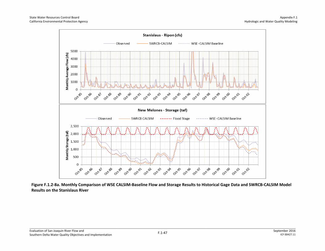
State Water Resources Control Board California Environmental Protection Agency
Appendix F.1 Hydrologic and Water Quality Modeling
Evaluation of San Joaquin River Flow and Southern Delta Water Quality Objectives and Implementation
F.1-47 September 2016
ICF 00427.11
Figure F.1.2-8a. Monthly Comparison of WSE CALSIM-Baseline Flow and Storage Results to Historical Gage Data and SWRCB-CALSIM Model Results on the Stanislaus River

State Water Resources Control Board California Environmental Protection Agency
Appendix F.1 Hydrologic and Water Quality Modeling
Evaluation of San Joaquin River Flow and Southern Delta Water Quality Objectives and Implementation
F.1-48 September 2016
ICF 00427.11
Figure F.1.2-8b. Monthly Comparison of WSE CALSIM-Baseline Flow and Storage Results to Historical Gage Data and SWRCB-CALSIM Model Results on the Tuolumne River
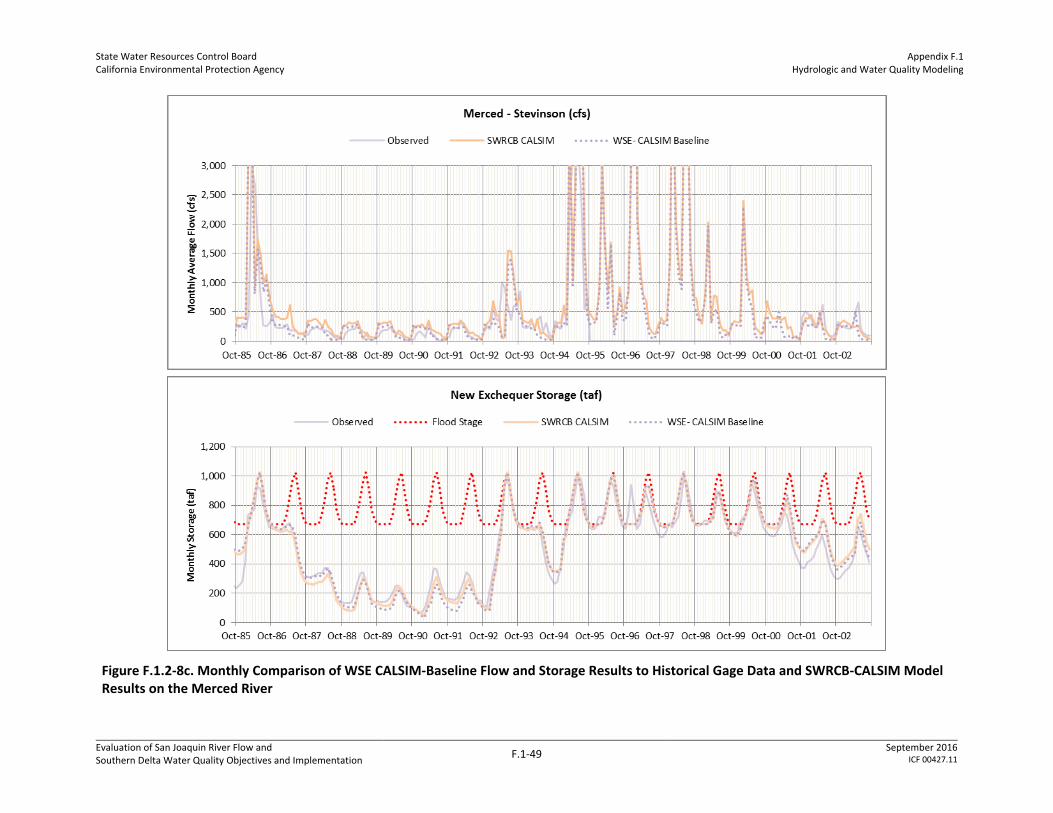
State Water Resources Control Board California Environmental Protection Agency
Appendix F.1 Hydrologic and Water Quality Modeling
Evaluation of San Joaquin River Flow and Southern Delta Water Quality Objectives and Implementation
F.1-49 September 2016
ICF 00427.11
Figure F.1.2-8c. Monthly Comparison of WSE CALSIM-Baseline Flow and Storage Results to Historical Gage Data and SWRCB-CALSIM Model Results on the Merced River

State Water Resources Control Board California Environmental Protection Agency
Appendix F.1 Hydrologic and Water Quality Modeling
Evaluation of San Joaquin River Flow and Southern Delta Water Quality Objectives and Implementation
F.1-50 September 2016
ICF 00427.11
Figure F.1.2-9. Comparison of WSE CALSIM-Baseline with SWRCB-CALSIM output on the Stanislaus River for (a) February–June Flow at Ripon, (b) End-of-September Storage, (c) Annual Diversion Delivery, (d) February–June at Ripon as a Percentage of Unimpaired Flow
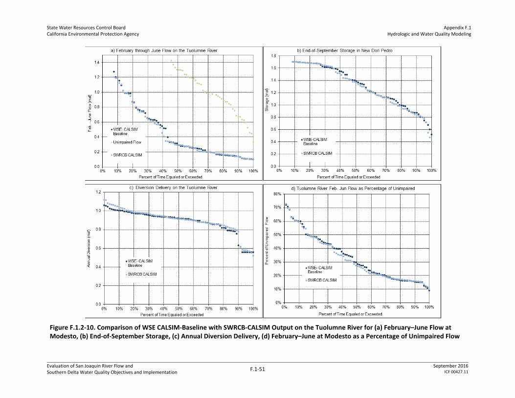
State Water Resources Control Board California Environmental Protection Agency
Appendix F.1 Hydrologic and Water Quality Modeling
Evaluation of San Joaquin River Flow and Southern Delta Water Quality Objectives and Implementation
F.1-51 September 2016
ICF 00427.11
Figure F.1.2-10. Comparison of WSE CALSIM-Baseline with SWRCB-CALSIM Output on the Tuolumne River for (a) February–June Flow at Modesto, (b) End-of-September Storage, (c) Annual Diversion Delivery, (d) February–June at Modesto as a Percentage of Unimpaired Flow

State Water Resources Control Board California Environmental Protection Agency
Appendix F.1 Hydrologic and Water Quality Modeling
Evaluation of San Joaquin River Flow and Southern Delta Water Quality Objectives and Implementation
F.1-52 September 2016
ICF 00427.11
Figure F.1.2-11. Comparison of WSE CALSIM-Baseline with SWRCB CALSIM Output on the Merced River for (a) February–June Flow at Stevinson, (b) End-of-September Storage, (c) Annual Diversion Delivery, (d) February–June Flow at Stevinson as a Percentage of Unimpaired Flow

State Water Resources Control Board California Environmental Protection Agency
Appendix F.1 Hydrologic and Water Quality Modeling
Evaluation of San Joaquin River Flow and Southern Delta Water Quality Objectives and Implementation
F.1-53 September 2016
ICF 00427.11
Figure F.1.2-12. Comparison of WSE CALSIM-Baseline with SWRCB-CALSIM Output for (a) Annual Diversion Delivery from All Three Major Tributaries, (b) Flow at Vernalis, (c) February–June Flow at Vernalis as a Percentage of Unimpaired Flow

State Water Resources Control Board California Environmental Protection Agency
Appendix F.1 Hydrologic and Water Quality Modeling
Evaluation of San Joaquin River Flow and Southern Delta Water Quality Objectives and Implementation
F.1-54 September 2016
ICF 00427.11
Figure F.1.2-13. Annual WSE CALSIM-Baseline Results for Stanislaus River Diversions, Flow, and Reservoir Operations Compared to SWRCB-CALSIM Results

State Water Resources Control Board California Environmental Protection Agency
Appendix F.1 Hydrologic and Water Quality Modeling
Evaluation of San Joaquin River Flow and Southern Delta Water Quality Objectives and Implementation
F.1-55 September 2016
ICF 00427.11
Figure F.1.2-14. Annual WSE CALSIM-Baseline Results for Tuolumne River Diversions, Flow, and Reservoir Operations Compared to SWRCB CALSIM Results

State Water Resources Control Board California Environmental Protection Agency
Appendix F.1 Hydrologic and Water Quality Modeling
Evaluation of San Joaquin River Flow and Southern Delta Water Quality Objectives and Implementation
F.1-56 September 2016
ICF 00427.11
Figure F.1.2-15. Annual WSE CALSIM-Baseline Results for Merced River Diversions, Flow, and Reservoir Operations Compared to SWRCB CALSIM Results
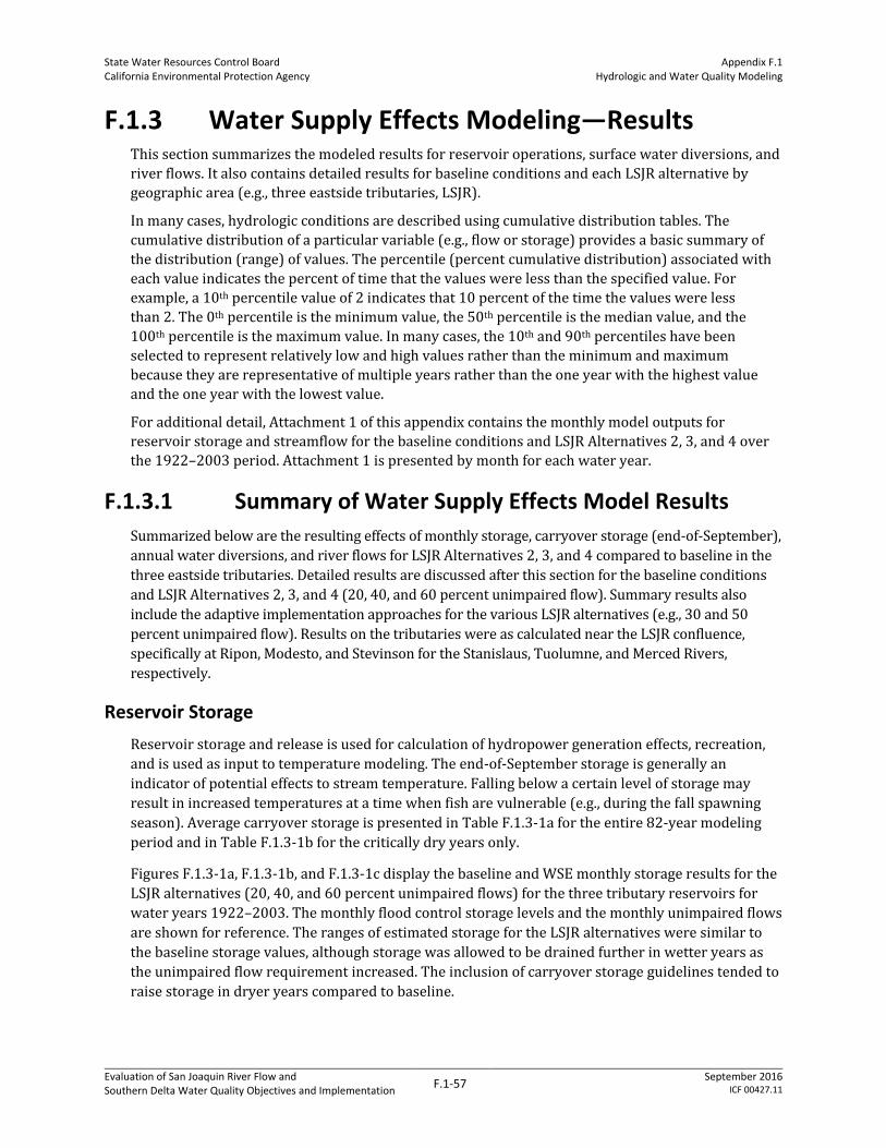
State Water Resources Control Board California Environmental Protection Agency
Appendix F.1 Hydrologic and Water Quality Modeling
Evaluation of San Joaquin River Flow and Southern Delta Water Quality Objectives and Implementation
F.1-57 September 2016
ICF 00427.11
F.1.3 Water Supply Effects Modeling—Results This section summarizes the modeled results for reservoir operations, surface water diversions, and
river flows. It also contains detailed results for baseline conditions and each LSJR alternative by
geographic area (e.g., three eastside tributaries, LSJR).
In many cases, hydrologic conditions are described using cumulative distribution tables. The
cumulative distribution of a particular variable (e.g., flow or storage) provides a basic summary of
the distribution (range) of values. The percentile (percent cumulative distribution) associated with
each value indicates the percent of time that the values were less than the specified value. For
example, a 10th percentile value of 2 indicates that 10 percent of the time the values were less
than 2. The 0th percentile is the minimum value, the 50th percentile is the median value, and the
100th percentile is the maximum value. In many cases, the 10th and 90th percentiles have been
selected to represent relatively low and high values rather than the minimum and maximum
because they are representative of multiple years rather than the one year with the highest value
and the one year with the lowest value.
For additional detail, Attachment 1 of this appendix contains the monthly model outputs for
reservoir storage and streamflow for the baseline conditions and LSJR Alternatives 2, 3, and 4 over
the 1922–2003 period. Attachment 1 is presented by month for each water year.
F.1.3.1 Summary of Water Supply Effects Model Results
Summarized below are the resulting effects of monthly storage, carryover storage (end-of-September),
annual water diversions, and river flows for LSJR Alternatives 2, 3, and 4 compared to baseline in the
three eastside tributaries. Detailed results are discussed after this section for the baseline conditions
and LSJR Alternatives 2, 3, and 4 (20, 40, and 60 percent unimpaired flow). Summary results also
include the adaptive implementation approaches for the various LSJR alternatives (e.g., 30 and 50
percent unimpaired flow). Results on the tributaries were as calculated near the LSJR confluence,
specifically at Ripon, Modesto, and Stevinson for the Stanislaus, Tuolumne, and Merced Rivers,
respectively.
Reservoir Storage
Reservoir storage and release is used for calculation of hydropower generation effects, recreation,
and is used as input to temperature modeling. The end-of-September storage is generally an
indicator of potential effects to stream temperature. Falling below a certain level of storage may
result in increased temperatures at a time when fish are vulnerable (e.g., during the fall spawning
season). Average carryover storage is presented in Table F.1.3-1a for the entire 82-year modeling
period and in Table F.1.3-1b for the critically dry years only.
Figures F.1.3-1a, F.1.3-1b, and F.1.3-1c display the baseline and WSE monthly storage results for the
LSJR alternatives (20, 40, and 60 percent unimpaired flows) for the three tributary reservoirs for
water years 1922–2003. The monthly flood control storage levels and the monthly unimpaired flows
are shown for reference. The ranges of estimated storage for the LSJR alternatives were similar to
the baseline storage values, although storage was allowed to be drained further in wetter years as
the unimpaired flow requirement increased. The inclusion of carryover storage guidelines tended to
raise storage in dryer years compared to baseline.
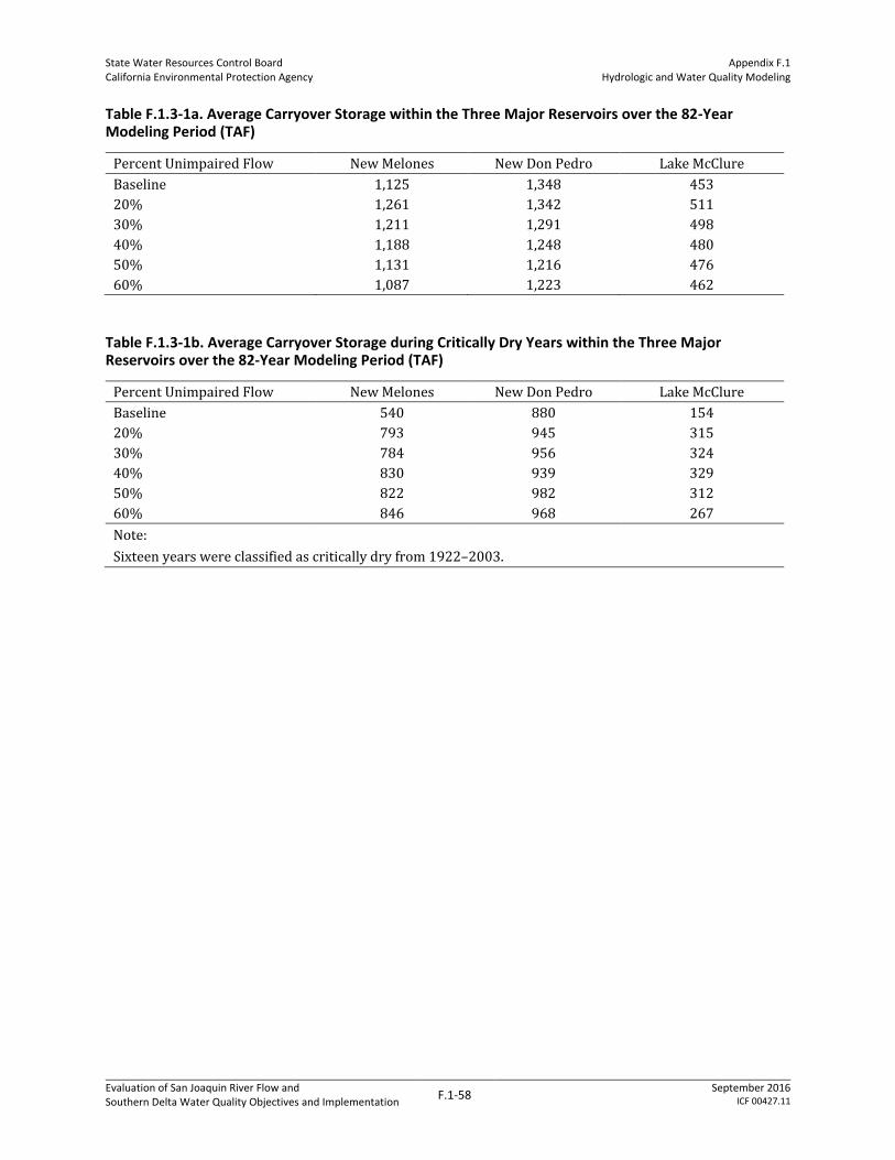
State Water Resources Control Board California Environmental Protection Agency
Appendix F.1 Hydrologic and Water Quality Modeling
Evaluation of San Joaquin River Flow and Southern Delta Water Quality Objectives and Implementation
F.1-58 September 2016
ICF 00427.11
Table F.1.3-1a. Average Carryover Storage within the Three Major Reservoirs over the 82-Year Modeling Period (TAF)
Percent Unimpaired Flow New Melones New Don Pedro Lake McClure
Baseline 1,125 1,348 453
20% 1,261 1,342 511
30% 1,211 1,291 498
40% 1,188 1,248 480
50% 1,131 1,216 476
60% 1,087 1,223 462
Table F.1.3-1b. Average Carryover Storage during Critically Dry Years within the Three Major Reservoirs over the 82-Year Modeling Period (TAF)
Percent Unimpaired Flow New Melones New Don Pedro Lake McClure
Baseline 540 880 154
20% 793 945 315
30% 784 956 324
40% 830 939 329
50% 822 982 312
60% 846 968 267
Note:
Sixteen years were classified as critically dry from 1922–2003.

State Water Resources Control Board California Environmental Protection Agency
Appendix F.1 Hydrologic and Water Quality Modeling
Evaluation of San Joaquin River Flow and Southern Delta Water Quality Objectives and Implementation
F.1-59 September 2016
ICF 00427.11
Figure F.1.3-1a. Comparison of Baseline Conditions and WSE Model Results for 20%, 40%, and 60% Unimpaired Flow (LSJR Alternatives 2–4): New Melones Reservoir Storage and Stanislaus River Unimpaired Flows for 1922–2003

State Water Resources Control Board California Environmental Protection Agency
Appendix F.1 Hydrologic and Water Quality Modeling
Evaluation of San Joaquin River Flow and Southern Delta Water Quality Objectives and Implementation
F.1-60 September 2016
ICF 00427.11
Figure F.1.3-1b. Comparison of Baseline Conditions and WSE Model Results for 20%, 40%, and 60% Unimpaired Flow (LSJR Alternatives 2–4): New Don Pedro Reservoir Storage and Tuolumne River Unimpaired Flows for 1922–2003

State Water Resources Control Board California Environmental Protection Agency
Appendix F.1 Hydrologic and Water Quality Modeling
Evaluation of San Joaquin River Flow and Southern Delta Water Quality Objectives and Implementation
F.1-61 September 2016
ICF 00427.11
Figure F.1.3-1c. Comparison of Baseline Conditions and WSE Model Results for 20%, 40%, and 60% Unimpaired Flow (LSJR Alternatives 2–4): Lake McClure Storage and Merced River Unimpaired Flows for 1922–2003

State Water Resources Control Board California Environmental Protection Agency
Appendix F.1 Hydrologic and Water Quality Modeling
Evaluation of San Joaquin River Flow and Southern Delta Water Quality Objectives and Implementation
F.1-62 September 2016
ICF 00427.11
River Flows
Table F.1.3-2a contains a summary of the average effects of the LSJR alternatives on river flows
(flow volumes, TAF) from February–June and annually as compared to the baseline flows for each
eastside tributary and near Vernalis on the SJR. Most of the change in flow volume associated with
implementation of the unimpaired flow objectives (in terms of TAF) occurred during the unimpaired
flow objective months (February–June). During the other months, the LSJR alternative flows were
similar to the baseline flows. Table F.1.3-2b summarizes the mean annual February–June instream
flow totals under Alternative 3 for each tributary in the plan area by water year type.
Figures F.1.3-2a, F.1.3-2b, F.1.3-2c, and F.1.3-2d show the simulated monthly flows in the Stanislaus,
Tuolumne, and Merced Rivers near the confluence with the LSJR and the SJR at Vernalis for water
years 1984–2003. The unimpaired flows are shown for comparison. The baseline flows were
generally low in many months each year until runoff was high enough to increase reservoir storage
and cause flood control releases (in wet years). From February–June, in general, as the percentage of
unimpaired flow increases, the resulting river flow increased. The simulated river flows are
described in more detail in Sections F.1.2.4 through F.1.2.7.
Table F.1.3-2a. Average Baseline Streamflow and Differences from Baseline Conditions on the Eastside Tributaries and near Vernalis
Percent Unimpaired Flow
Stanislaus River near Ripon (TAF)/(%)
Tuolumne River near Modesto
(TAF)/(%)
Merced River near Stevinson
(TAF)/(%)
Total three tributaries (TAF)/(%)
SJR near Vernalis
(TAF)/(%)
February–June Average
Baseline 312/100 562/100 245/100 1,116/100 1,742/100
20% -3/-1 32/6 27/11 56/5 56/3
25% 11/4 53/10 42/17 106/10 106/6
30% 27/9 85/15 62/26 174/16 174/10
35% 30/9 98/17 70/29 197/18 197/11
40% 62/20 135/24 91/38 288/26 288/17
45% 91/29 171/30 111/46 373/33 373/21
50% 128/41 220/39 137/57 485/43 485/28
55% 164/53 271/48 163/67 598/54 598/34
60% 203/65 332/59 193/80 728/65 728/42
Annual Average
Baseline 549/100 895/100 454/100 1,897/100 2,965/100
20% 5/1 23/3 31/7 59/3 59/2
25% 15/1 37/4 42/9 94/5 94/3
30% 28/5 63/7 58/13 149/8 149/5
35% 42/8 90/10 74/16 206/11 206/7
40% 74/13 127/14 93/21 294/15 294/10

State Water Resources Control Board California Environmental Protection Agency
Appendix F.1 Hydrologic and Water Quality Modeling
Evaluation of San Joaquin River Flow and Southern Delta Water Quality Objectives and Implementation
F.1-63 September 2016
ICF 00427.11
Percent Unimpaired Flow
Stanislaus River near Ripon (TAF)/(%)
Tuolumne River near Modesto
(TAF)/(%)
Merced River near Stevinson
(TAF)/(%)
Total three tributaries (TAF)/(%)
SJR near Vernalis
(TAF)/(%)
45% 94/17 159/18 110/24 363/19 363/12
50% 132/24 202/23 135/30 469/25 469/16
55% 163/30 249/28 158/35 571/30 571/19
60% 202/37 307/34 184/41 693/37 693/23
Notes:
Resulting flow effects on the tributaries were as calculated near the LSJR confluence, specifically at Ripon, Modesto, and Stevinson for the Stanislaus, Tuolumne, and Merced Rivers, respectively.
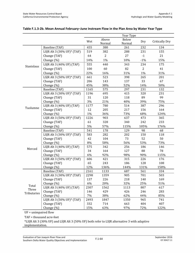
State Water Resources Control Board California Environmental Protection Agency
Appendix F.1 Hydrologic and Water Quality Modeling
Evaluation of San Joaquin River Flow and Southern Delta Water Quality Objectives and Implementation
F.1-64 September 2016
ICF 00427.11
Table F.1.3-2b. Mean Annual February–June Instream Flow in the Plan Area by Water Year Type
Year Type
Wet Above
Normal Below
Normal Dry Critically Dry
Stanislaus
Baseline (TAF) 455 380 261 232 134
LSJR Alt 3 (30% UF)* (TAF) 519 382 288 231 155
Change (TAF) 64 2 27 -1 21
Change (%) 14% 1% 10% -1% 15%
LSJR Alt 3 (40% UF) (TAF) 555 440 343 234 175
Change (TAF) 100 60 82 2 41
Change (%) 22% 16% 31% 1% 31%
LSJR Alt 3 (50% UF)* (TAF) 661 523 398 265 201
Change (TAF) 206 143 137 33 67
Change (%) 45% 38% 52% 14% 50%
Tuolumne
Baseline (TAF) 1165 575 297 231 132
LSJR Alt 3 (30% UF)* (TAF) 1196 695 415 320 231
Change (TAF) 31 120 118 89 99
Change (%) 3% 21% 40% 39% 75%
LSJR Alt 3 (40% UF) (TAF) 1177 780 514 387 296
Change (TAF) 12 205 217 156 164
Change (%) 1% 36% 73% 68% 124%
LSJR Alt 3 (50% UF)* (TAF) 1226 903 637 473 365
Change (TAF) 61 328 340 242 233
Change (%) 5% 57% 115% 105% 176%
Merced
Baseline (TAF) 541 178 129 98 68
LSJR Alt 3 (30% UF)* (TAF) 583 282 202 150 118
Change (TAF) 42 104 73 52 50
Change (%) 8% 58% 56% 53% 73%
LSJR Alt 3 (40% UF) (TAF) 575 342 256 186 146
Change (TAF) 34 164 127 88 78
Change (%) 6% 92% 98% 90% 115%
LSJR Alt 3 (50% UF)* (TAF) 606 421 315 226 176
Change (TAF) 65 243 186 128 108
Change (%) 12% 136% 144% 131% 158%
Total Three
Tributaries
Baseline (TAF) 2161 1133 687 561 334
LSJR Alt 3 (30% UF)* (TAF) 2298 1359 905 701 503
Change (TAF) 137 226 218 140 169
Change (%) 6% 20% 32% 25% 51%
LSJR Alt 3 (40% UF) (TAF) 2307 1562 1113 807 617
Change (TAF) 146 429 426 246 283
Change (%) 7% 38% 62% 44% 85%
LSJR Alt 3 (50% UF)* (TAF) 2493 1847 1350 965 741
Change (TAF) 332 714 663 404 407
Change (%) 15% 63% 97% 72% 122%
UF = unimpaired flow
TAF = thousand acre-feet
*LSJR Alt 3 (30% UF) and LSJR Alt 3 (50% UF) both refer to LSJR alternative 3 with adaptive implementation.

State Water Resources Control Board California Environmental Protection Agency
Appendix F.1 Hydrologic and Water Quality Modeling
Evaluation of San Joaquin River Flow and Southern Delta Water Quality Objectives and Implementation
F.1-65 September 2016
ICF 00427.11
Figure F.1.3-2a. Comparison of Monthly Stanislaus River Flows for Baseline Conditions and 20%, 40%, and 60% Unimpaired Flow (LSJR Alternatives 2–4) for Water Years 1984–2003

State Water Resources Control Board California Environmental Protection Agency
Appendix F.1 Hydrologic and Water Quality Modeling
Evaluation of San Joaquin River Flow and Southern Delta Water Quality Objectives and Implementation
F.1-66 September 2016
ICF 00427.11
Figure F.1.3-2b. Comparison of Monthly Tuolumne River Flows for Baseline Conditions and 20%, 40%, and 60% Unimpaired Flow (LSJR Alternatives 2–4) for Water Years 1984–2003
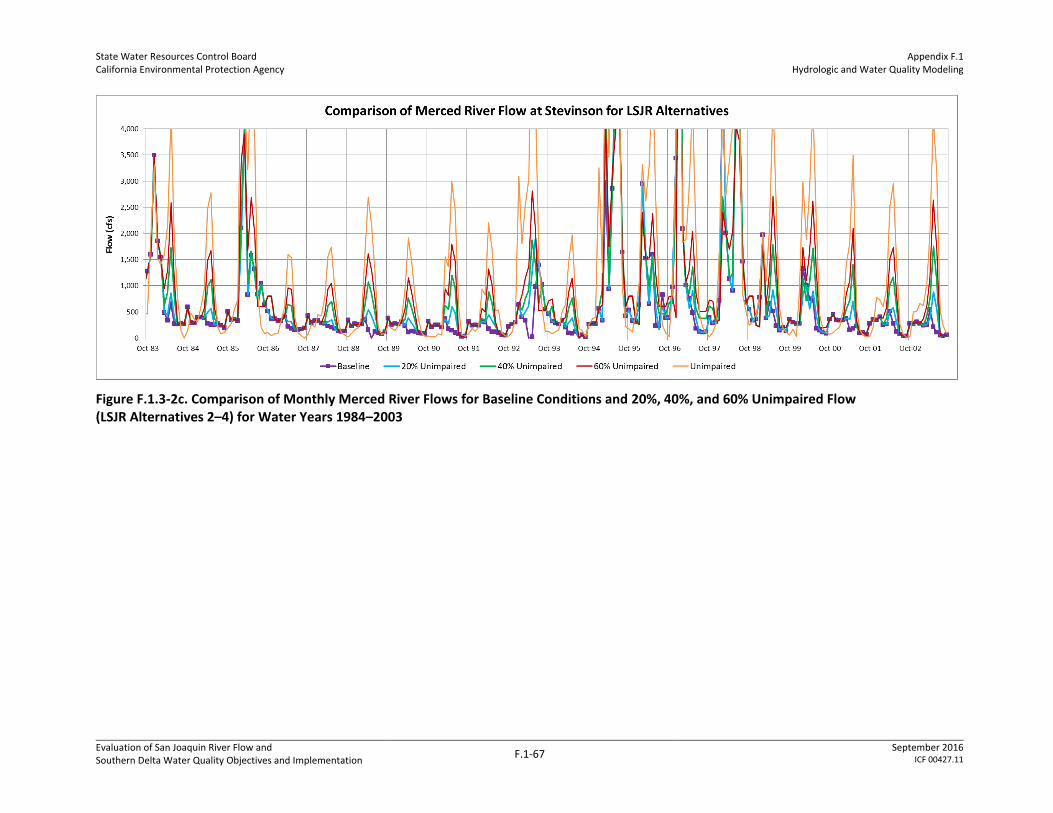
State Water Resources Control Board California Environmental Protection Agency
Appendix F.1 Hydrologic and Water Quality Modeling
Evaluation of San Joaquin River Flow and Southern Delta Water Quality Objectives and Implementation
F.1-67 September 2016
ICF 00427.11
Figure F.1.3-2c. Comparison of Monthly Merced River Flows for Baseline Conditions and 20%, 40%, and 60% Unimpaired Flow (LSJR Alternatives 2–4) for Water Years 1984–2003

State Water Resources Control Board California Environmental Protection Agency
Appendix F.1 Hydrologic and Water Quality Modeling
Evaluation of San Joaquin River Flow and Southern Delta Water Quality Objectives and Implementation
F.1-68 September 2016
ICF 00427.11
Figure F.1.3-2d. Comparison of Monthly SJR at Vernalis Flows for Baseline Conditions and 20%, 40%, and 60% Unimpaired Flow (LSJR Alternatives 2–4) for Water Years 1984–2003

State Water Resources Control Board California Environmental Protection Agency
Appendix F.1 Hydrologic and Water Quality Modeling
Evaluation of San Joaquin River Flow and Southern Delta Water Quality Objectives and Implementation
F.1-69 September 2016
ICF 00427.11
Surface Water Diversions
Table F.1.3-3 contains a summary of the effects on diversions for each eastside tributary and for the
plan area of the LSJR alternatives as compared to the baseline for the 82-year modeling period.
Tables F.1.3-4a, F.1.3-4b, and F.1.3-4c show the annual cumulative distributions of water supply
diversions under the LSJR alternatives as compared to the baseline water supply diversions and
deficits indicators for each tributary. The deficit indicator was calculated as maximum demand
minus delivery, where the maximum demand equals the maximum annual diversion under baseline
conditions. It should be noted, however, that in some years (particularly wet years), the demand is
lower than in other years, so the deficit indicator could be an overprediction of the actual deficit. The
annual values are summarized with the minimum and maximum and average, as well as the 10
percent increments of the distribution of values. The range of annual unimpaired flow for each
tributary is shown for comparison. Additional details are discussed in Sections F.1.2.4 through
F.1.2.7 for baseline and LSJR Alternatives 2, 3, and 4.
Table F.1.3-3. Average Annual Baseline Water Supply and Difference from Baseline Conditions on the Eastside Tributaries and Plan Area Totals over the 82-year Modeling Period
Percent Unimpaired Flow Requirement
Stanislaus Diversion
(TAF)/(% of Baseline)
Tuolumne Diversion
(TAF)/(% of Baseline)
Merced Diversion
(TAF)/(% of Baseline)
Total Three Tributaries
(TAF)/(% of Baseline)
Baseline 637/100 851/100 580/100 2,068/100
20% -12/-2 -20/-2 -33/-6 -65/-3
25% -20/-3 -32/-4 -44/-8 -96/-5
30% -33/-5 -56/-7 -60/-10 -149/-7
35% -45/-7 -82/-10 -75/-13 -202/-10
40% -79/-12 -119/-14 -95/-16 -293/-14
45% -97/-15 -149/-18 -111/-19 -357/-17
50% -136/-21 -193/-23 -136/-23 -465/-23
55% -167/-26 -240/-28 -159/-27 -566/-27
60% -206/-32 -298/-35 -185/-32 -689/-33
Annual Summary of Results
Baseline and the LSJR alternatives for each tributary are summarized with the distribution of the
annual carryover storage (end-of-September), the distribution of annual water supply deliveries, and
the distribution of annual or February–June river flows (volume and percentage of unimpaired flow).
Tables F.1.3-4a, F.1.3-4b, and F.1.3-4c present the cumulative distributions for annual diversions and
annual diversion deficits on the Stanislaus, Tuolumne, and Merced Rivers, respectively. Table F.1.3-4d
illustrates the variation of diversion by water year type under LSJR Alternative 3.

State Water Resources Control Board California Environmental Protection Agency
Appendix F.1 Hydrologic and Water Quality Modeling
Evaluation of San Joaquin River Flow and Southern Delta Water Quality Objectives and Implementation
F.1-70 September 2016
ICF 00427.11
Table F.1.3-4a. Annual Water Supply Diversions for Baseline Conditions and Percent of Unimpaired Flow on the Stanislaus
Unimpaired Flow
Stanislaus Diversions (TAF) Stanislaus Deficit Indicator (TAF)
Baseline 20% 30% 40% 50% 60% Baseline 20% 30% 40% 50% 60%
Minimum 155 252 228 228 228 198 164 520 544 544 544 574 607
10% 456 538 452 320 265 222 201 234 320 452 507 550 571
20% 592 583 570 508 403 288 221 189 202 264 369 484 551
30% 680 605 624 616 464 333 260 167 148 156 307 439 511
40% 891 630 657 640 584 461 322 142 115 132 188 311 450
50% 1,095 661 673 664 640 575 399 111 99 108 132 196 373
60% 1,264 676 687 681 663 630 510 96 85 91 109 142 262
70% 1,368 694 701 697 679 663 601 78 71 75 93 109 171
80% 1,563 708 709 708 695 681 661 64 63 63 77 91 111
90% 1,910 723 724 724 712 705 690 49 48 48 60 67 82
Maximum 2,954 772 772 772 759 759 759 0 0 0 13 13 13
Average 1,118 637 624 604 558 500 431 135 147 168 214 271 341
Table F.1.3-4b. Annual Water Supply Diversions for Baseline Conditions and Percent of Unimpaired Flow on the Tuolumne
Unimpaired Flow
Tuolumne Diversions (TAF) Tuolumne Deficit Indicator (TAF)
Baseline 20% 30% 40% 50% 60% Baseline 20% 30% 40% 50% 60%
Minimum 384 557 371 371 341 215 214 477 663 663 693 819 820
10% 836 685 652 543 408 322 229 349 382 491 625 712 805
20% 1,055 796 781 715 563 395 287 237 253 319 471 639 747
30% 1,166 828 822 777 641 511 378 205 211 257 393 523 656
40% 1,413 855 852 823 763 652 460 179 182 211 271 382 574
50% 1,783 878 869 851 802 751 538 156 165 183 232 283 496
60% 2,036 891 889 871 828 802 673 143 145 163 206 231 361
70% 2,198 915 910 890 859 828 763 119 124 144 175 206 271
80% 2,490 932 930 911 887 857 820 102 104 123 147 177 214
90% 3,090 960 957 938 908 890 853 74 77 96 126 144 181
Maximum 4,630 1,034 1,034 1,004 1,004 1,004 907 0 0 30 30 30 127
Average 1,851 851 831 795 732 657 553 183 203 239 302 376 481

State Water Resources Control Board California Environmental Protection Agency
Appendix F.1 Hydrologic and Water Quality Modeling
Evaluation of San Joaquin River Flow and Southern Delta Water Quality Objectives and Implementation
F.1-71 September 2016
ICF 00427.11
Table F.1.3-4c. Annual Water Supply Diversions for Baseline Conditions and Percent of Unimpaired Flow on the Merced
Unimpaired Flow
Merced Diversions (TAF) Merced Deficit Indicator (TAF)
Baseline 20% 30% 40% 50% 60% Baseline 20% 30% 40% 50% 60%
Minimum 151 136 203 203 203 202 202 543 476 476 476 478 478
10% 408 441 380 308 259 231 220 239 299 372 420 448 459
20% 489 558 472 407 353 300 243 122 208 273 326 380 437
30% 560 578 551 495 408 330 284 102 129 185 272 350 396
40% 669 602 565 537 467 387 323 78 114 143 212 293 357
50% 895 617 587 560 551 482 380 63 92 120 128 198 299
60% 1,086 630 603 582 564 522 442 50 77 98 116 158 238
70% 1,169 643 619 611 582 558 494 37 61 69 97 122 186
80% 1,399 653 632 627 607 579 557 26 48 53 73 100 122
90% 1,706 669 659 642 632 610 580 10 21 37 48 70 100
Maximum 2,790 680 673 673 673 668 648 0 7 7 7 12 32
Average 958 580 547 520 485 444 395 100 133 160 194 235 284

State Water Resources Control Board California Environmental Protection Agency
Appendix F.1 Hydrologic and Water Quality Modeling
Evaluation of San Joaquin River Flow and Southern Delta Water Quality Objectives and Implementation
F.1-72 September 2016
ICF 00427.11
Table F.1.3-4d. Mean Annual Diversions Under 40 Percent Unimpaired Flow Proposal by Water Year Type
Year Type
Wet Above Normal Below Normal Dry Critically Dry
Stanislaus Baseline (TAF) 661 661 661 683 520
LSJR Alt 3 (40% UF) (TAF) 662 630 613 536 303
Change (TAF) 1 -31 -48 -147 -217
Change (%) 0% -5% -7% -22% -42%
Tuolumne Baseline (TAF) 848 882 931 938 689
LSJR Alt 3 (40%UF) (TAF) 845 855 800 681 426
Change (TAF) -3 -27 -131 -257 -263
Change (%) 0% -3% -14% -27% -38%
Merced Baseline (TAF) 591 622 642 650 416
LSJR Alt 3 (40% UF) (TAF) 591 607 508 381 272
Change (TAF) 0 -15 -134 -268 -144
Change (%) 0% -2% -21% -41% -35%
Total Three Tributaries
Baseline (TAF) 2,099 2,164 2,233 2,271 1,625
LSJR Alt 3 (40% UF) (TAF) 2,097 2,091 1,921 1,598 1,001
Change (TAF) -2 -73 -313 -673 -624
Change (%) 0% -3% -14% -30% -38%
UF = percent of unimpaired flow
TAF = thousand acre-feet
State Water Resources Control Board California Environmental Protection Agency
Appendix F.1 Hydrologic and Water Quality Modeling
Evaluation of San Joaquin River Flow and Southern Delta Water Quality Objectives and Implementation
F.1-73 September 2016
ICF 00427.11
Figures F.1.3-3a, F.1.3-3b, F.1.3-3c, and, F.1.3-3d show the summary of annual results on the Stanislaus
River. This compares the distribution of annual (a) February–June flow volume, (b) end-of-September
storage, (c) diversion volume from the river, and (d) February–June flow as a percentage of
unimpaired flow. The Stanislaus River February–June flow volumes were slightly reduced from
baseline flows for LSJR Alternative 2 (20 percent unimpaired flow), were higher for LSJR Alternative 3
(40 percent unimpaired flow), and were much increased for LSJR Alternative 4 (60 percent
unimpaired flow). As seen in Figure F.1.3-3d, the percentage of unimpaired flow does not always meet
the percentage specified by the alternatives (LSJR Alternatives 3 and 4, specifically). This is because a
portion of the flow from February–June in wet years was shifted to later in the year as part of adaptive
implementation for controlling potential temperature effects during that time of year. End-of-
September storage generally tended to be reduced slightly as a result of the LSJR alternatives,
primarily during the wetter years (with the reduction increasing with the amount of unimpaired flow
released), except in the driest years, when the carryover storage guidelines resulted in higher
carryover storage for the LSJR alternatives compared with baseline conditions. The distribution of
annual deliveries was decreased slightly for LSJR Alternative 2, reduced for LSJR Alternative 3, and
reduced substantially for LSJR Alternative 4 in the majority of years compared with baseline
conditions.
Figures F.1.3-4a, F.1.3-4b, F.1.3-4c, and F.1.3-4d show the summary of annual results on the
Tuolumne River. This compares the distribution of (a) annual February–June flow, (b) end-of-
September storage, (c) annual water supply diversions from the three tributaries, and (d) flow as a
percentage of unimpaired flow. The Tuolumne River February–June flow volumes were generally
slightly greater than the baseline flows for LSJR Alternative 2 (20 percent unimpaired flow), were
increased for LSJR Alternative 3 (40 percent unimpaired flow), and were increased more for LSJR
Alternative 4 (60 percent unimpaired flow). As can be seen in Figure F.1-20d, the percentage of
unimpaired flow does not always meet the percentage specified by the alternatives (LSJR
Alternatives 3 and 4 specifically). This is because there is a portion of the flow from February–June
in wet years that shifts to later in the year as part of adaptive implementation for controlling
potential temperature effects during that time of year. End-of-September storage generally tended
to be reduced slightly as a result of the LSJR alternatives primarily during the wetter years (with the
reduction increasing with the amount of unimpaired flow released), except in the driest years when
the carryover storage guidelines resulted in higher carryover storage for the LSJR alternatives than
baseline. The distribution of annual deliveries was decreased slightly for LSJR Alternative 2, was
reduced for LSJR Alternative 3, and was reduced substantially for LSJR Alternative 4 in the majority
of years compared to the baseline conditions.
Figures F.1.3-5a, F.1.3-5b, F.1.3-5c, and F.1.3-5d show the summary of annual results on the Merced
River. This compares the distribution of (a) annual February–June flow, (b) end-of-September
storage, (c) annual water supply diversions from the three tributaries, and (d) flow as a percentage
of unimpaired flow. The Merced River February–June flow volumes were slightly increased from the
baseline flows for LSJR Alternative 2 (20 percent unimpaired flow), were increased for LSJR
Alternative 3 (40 percent unimpaired flow), and were increased more for LSJR Alternative 4 (60
percent unimpaired flow). As can be seen in Figure F.1-21d, the percentage of unimpaired flow does
not always meet the percentage specified by the alternatives (LSJR Alternatives 3 and 4 specifically).
This is because there is a portion of the flow from February–June in wet and above-normal years
that shifts as part of adaptive implementation to later in the year for controlling potential
temperature effects during that time of year. End-of-September storage generally tended to be
reduced slightly as a result of the LSJR alternatives primarily during the wetter years (with the
reduction increasing with the amount of unimpaired flow released), except in the driest years when
State Water Resources Control Board California Environmental Protection Agency
Appendix F.1 Hydrologic and Water Quality Modeling
Evaluation of San Joaquin River Flow and Southern Delta Water Quality Objectives and Implementation
F.1-74 September 2016
ICF 00427.11
the carryover storage guidelines resulted in higher carryover storage for the LSJR alternatives than
baseline. The distribution of annual deliveries was decreased slightly for LSJR Alternative 2, was
reduced for LSJR Alternative 3, and was reduced substantially for LSJR Alternative 4 in the majority
of years compared to the baseline conditions.

State Water Resources Control Board California Environmental Protection Agency
Appendix F.1 Hydrologic and Water Quality Modeling
Evaluation of San Joaquin River Flow and Southern Delta Water Quality Objectives and Implementation
F.1-75 September 2016
ICF 00427.11
Figure F.1.3-3. Stanislaus River Annual Distributions from 1922–2003 of (a) February–June Flow Volume, (b) End-of-September Storage, (c) Annual Diversion Delivery, and (d) February–June Flow Volume as a Percentage of Unimpaired Flow

State Water Resources Control Board California Environmental Protection Agency
Appendix F.1 Hydrologic and Water Quality Modeling
Evaluation of San Joaquin River Flow and Southern Delta Water Quality Objectives and Implementation
F.1-76 September 2016
ICF 00427.11
Figure F.1.3-4. Tuolumne River Annual Distributions from 1922–2003 of (a) February–June Flow Volume, (b) End-of-September Storage, (c) Annual Diversion Delivery, and (d) February–June Flow Volume as a Percentage of Unimpaired Flow

State Water Resources Control Board California Environmental Protection Agency
Appendix F.1 Hydrologic and Water Quality Modeling
Evaluation of San Joaquin River Flow and Southern Delta Water Quality Objectives and Implementation
F.1-77 September 2016
ICF 00427.11
Figure F.1.3-5. Merced River Annual Distributions from 1922–2003 of (a) February–June Flow Volume, (b) End-of-September Storage, (c) Annual Diversion Delivery, and (d) February–June Flow Volume as a Percentage of Unimpaired Flow
State Water Resources Control Board California Environmental Protection Agency
Appendix F.1 Hydrologic and Water Quality Modeling
Evaluation of San Joaquin River Flow and Southern Delta Water Quality Objectives and Implementation
F.1-78 September 2016
ICF 00427.11
Figures F.1.3-6a, F.1.3-6b, and F.1.3-6c show the summary of annual results on the SJR at Vernalis. This
compares the distribution of (a) annual February–June Flow, (b) annual water supply diversions from
the plan area, and (c) flow as a percentage of unimpaired flow. The SJR at Vernalis February–June flow
volumes were generally similar to the baseline flows for LSJR Alternative 2, were increased for LSJR
Alternative 3, and were increased more for LSJR Alternative 4. Because the flow at Vernalis is also
dependent on flow from the Upper SJR, the resulting flow at Vernalis did not reach the full percentage
set out by LSJR Alternatives 3 and 4 as well as it was reached in the three tributaries.

State Water Resources Control Board California Environmental Protection Agency
Appendix F.1 Hydrologic and Water Quality Modeling
Evaluation of San Joaquin River Flow and Southern Delta Water Quality Objectives and Implementation
F.1-79 September 2016
ICF 00427.11
Figure F.1.3-6. SJR Annual Distributions from 1922–2003 of (a) Annual Three Tributary Diversion Delivery, (b) February–June Flow Volume near Vernalis, and (c) February–June Flow Volume near Vernalis as a Percentage of Unimpaired Flow

State Water Resources Control Board California Environmental Protection Agency
Appendix F.1 Hydrologic and Water Quality Modeling
Evaluation of San Joaquin River Flow and Southern Delta Water Quality Objectives and Implementation
F.1-80 September 2016
ICF 00427.11
F.1.3.2 Characterization of Baseline Conditions
Baseline conditions were simulated with the WSE model, as previously described, using historical
hydrology from 1922–2003 assuming regulatory conditions described in Section F.1.2.2,
Development of WSE Baseline and LSJR Alternative Conditions. This section compares baseline to the
three LSJR alternatives. The SJR upstream of the Merced River confluence was assumed to remain
unchanged and equal to the baseline conditions for LSJR Alternatives 2, 3, and 4.
Upper and Middle SJR
For baseline conditions and all alternatives, flows in the SJR upstream of the Merced River were
assumed to be equal to those simulated by the CALSIM case discussed in Section F.1.2.1, Water
Supply Effects Methods. Table F.1.3-5a shows the monthly and annual cumulative distributions for
the CALSIM simulated SJR flows upstream of the Merced River. This flow originates from upstream
releases at Friant Dam or from the Fresno and Chowchilla Rivers, local runoff from the Bear River in
the vicinity of Merced, wetlands releases from the Grasslands Wildlife Management Area refuges,
and agricultural drainage from irrigated lands in this upstream portion of the SJR watershed. The
CALSIM model estimated monthly flows that were nearly identical in more than 50 percent of the
years (clearly assumed values) with median monthly flows that were less than 500 cubic feet per
second (cfs) in most months and less than 1,000 cfs in all months.

State Water Resources Control Board California Environmental Protection Agency
Appendix F.1 Hydrologic and Water Quality Modeling
Evaluation of San Joaquin River Flow and Southern Delta Water Quality Objectives and Implementation
F.1-81 September 2016
ICF 00427.11
Table F.1.3-5a. Baseline Monthly Cumulative Distributions of SJR above the Merced Flow (cfs) for 1922–2003
OCT NOV DEC JAN FEB MAR APR MAY JUN JUL AUG SEP Annual (TAF)
SJR above Merced Flow (cfs)
Minimum 184 341 297 230 511 275 148 220 219 196 179 470 215
10% 193 396 378 285 565 447 247 284 296 248 198 485 259
20% 234 460 379 301 619 495 325 354 312 248 225 614 291
30% 234 460 396 334 655 528 369 443 329 264 225 614 304
40% 234 476 412 366 738 632 414 481 346 264 225 614 323
50% 237 477 428 423 864 702 555 510 380 264 225 614 367
60% 251 521 461 513 1,026 934 703 554 407 274 225 614 488
70% 251 595 516 800 1,477 1,213 843 633 452 296 241 614 552
80% 251 651 630 1,533 2,751 1,750 1,442 826 514 313 241 631 977
90% 266 765 1,096 2,353 6,149 4,604 4,696 4,660 1,889 360 256 631 1,583
Maximum 713 3,531 8,657 22,173 15,188 16,113 12,031 10,642 10,639 5,312 290 648 5,604
Average 246 612 885 1,355 2,136 1,759 1,511 1,356 948 472 228 604 726
Note:
This is the same for all LSJR alternatives as these alternatives are not modifying the flow above the confluence of the LSJR and the Merced River and this is outside the plan area. Please see Chapter 3, Alternatives Description, for more information.

State Water Resources Control Board California Environmental Protection Agency
Appendix F.1 Hydrologic and Water Quality Modeling
Evaluation of San Joaquin River Flow and Southern Delta Water Quality Objectives and Implementation
F.1-82 September 2016
ICF 00427.11
Merced River
Figure F.1-7a illustrates the basic water supply need for seasonal storage in Lake McClure to
increase the water supply delivery in the summer months when the unimpaired runoff is less than
the monthly demands for irrigation water. The water delivery target was compared to the
distribution of unimpaired flow values, which are shown as 10th, 30th, 50th, 70th, and 90th percentiles.
Because agricultural use requires a specified monthly pattern of water deliveries to satisfy crop
needs (transpiration), seasonal storage is needed to extend the period when unimpaired runoff
could be (directly) diverted for irrigation. For the Merced River, the average monthly demands were
less than or equal to the 10 percent cumulative monthly runoff from November through May. The
average June demand was between 30 and 50 percent cumulative runoff, and the average monthly
demands for July through October were greater than the 90 percent cumulative runoff. This
indicates that reservoir storage is needed to satisfy the June demand in about 30 to 50 percent of the
years, and reservoir storage is needed in more than 90 percent of the years to satisfy the July–
October demands.
0
50
100
150
200
250
300
350
400
450
OCT NOV DEC JAN FEB MAR APR MAY JUN JUL AUG SEP
Flo
w V
olu
me
(TA
F)
Merced Unimpaired Runoff and Diversion Target
10% 30% 50% 70% 90% Diversion Target
Figure F.1.3-7a. Monthly Merced River Unimpaired Runoff Compared to Average Monthly Water Supply Demands
Because there are no significant reservoirs or diversions in the Merced River watershed upstream of
Lake McClure, the inflow to Lake McClure is the Merced unimpaired runoff. Table F.1.3-5b shows the
monthly cumulative distributions for the baseline simulated Lake McClure storage (TAF). These
monthly storage patterns are similar to the historical storage observed since the New Exchequer
Dam was completed in 1965. The maximum storage of 1,024 TAF was simulated in about 30 percent
of the years in June. Storage was limited for flood control in the other months. The maximum storage
was 675 TAF from October–February. The median monthly storage levels were more than 400 TAF

State Water Resources Control Board California Environmental Protection Agency
Appendix F.1 Hydrologic and Water Quality Modeling
Evaluation of San Joaquin River Flow and Southern Delta Water Quality Objectives and Implementation
F.1-83 September 2016
ICF 00427.11
in all months and more than 600 TAF February–July. The minimum carryover storage (end-of-
September) was 81 TAF (12 percent of capacity), the 10 percent cumulative carryover storage was
126 TAF (18 percent of capacity) and the 20 percent cumulative carryover storage was 186 TAF (27
percent of capacity). The 50 percent cumulative (or median) carryover storage was above 451 TAF
(64 percent of capacity).
Table F.1.3-5b. Simulated Baseline Monthly Cumulative Distributions of Lake McClure Storage for 1922–2003
OCT NOV DEC JAN FEB MAR APR MAY JUN JUL AUG SEP
Lake McClure Storage (TAF)
Minimum 56 39 56 46 31 24 23 39 67 94 97 81
10% 98 91 87 100 144 157 227 261 260 197 149 126
20% 155 163 193 208 276 273 329 401 412 319 235 186
30% 253 259 287 311 372 398 439 546 518 420 334 283
40% 350 348 389 440 484 506 584 650 617 516 407 365
50% 430 436 465 552 638 654 663 710 703 606 503 451
60% 573 588 611 635 674 680 721 831 854 755 667 616
70% 656 643 650 669 675 723 773 940 983 889 770 700
80% 666 662 665 675 675 735 818 970 1,024 910 770 700
90% 674 675 675 675 675 735 845 970 1,024 910 770 700
Maximum 675 675 675 675 675 735 845 970 1,024 910 770 700
Average 424 423 437 462 494 529 583 680 697 605 505 453
Figure F.1.3-7b shows the Lake McClure carryover storage for the baseline conditions compared to
carryover storage for the simulated 20, 40, and 60 percent unimpaired flow. The baseline results
reflect the historical periods of low runoff (reduced storage) and the periods of high runoff (with
maximum carryover storage of 700 TAF). Many of the carryover storage values are at the maximum
allowed storage for flood control.
Figure F.1.3-7b. Lake McClure Carryover Storage (TAF) for Baseline Conditions and 20%, 40%, and 60% Unimpaired Flow (LSJR Alternatives 2–4) for 1922–2003

State Water Resources Control Board California Environmental Protection Agency
Appendix F.1 Hydrologic and Water Quality Modeling
Evaluation of San Joaquin River Flow and Southern Delta Water Quality Objectives and Implementation
F.1-84 September 2016
ICF 00427.11
The Lake McClure storage values correspond to surface elevations that can be calculated with a
simple stage-storage equation of the form:
Lake McClure Elevation = (Storage/Ks) ^ (1/b) (Eqn. F.1-11)
Where:
Elevation = feet above mean sea level (MSL)
Storage = reservoir storage in TAF
Ks = 1.665E-15 for storage ≥ 240 TAF and 3.068E-20 for storage < 240 TAF
b = 6.055 for storage ≥ 240 TAF and 7.709 for storage < 240 TAF
The equation coefficients Ks and b were based on the reservoir geometry (i.e., elevation, surface
area, volume).
The surface elevation is an important variable for evaluating hydroelectric energy generation at the
dam, boat dock access and recreation uses, reservoir fish habitat, and exposure of cultural resources
during extreme drawdown periods. Using this equation, the storages can be converted to surface
elevations for these resource evaluations. The surface elevation is about 617 feet for a storage
volume of 100 TAF (10 percent of maximum storage), 676 feet for a storage volume of 200 TAF
(20 percent of maximum storage), and about 770 feet for a storage volume of 500 TAF (50 percent
of maximum storage). The elevation is about 867 feet for a maximum storage of 1,024 TAF. Table
F.1.3-5c shows the monthly cumulative distributions of Lake McClure water surface elevations (feet
MSL) for the baseline.
Table F.1.3-5c. Simulated Baseline Monthly Cumulative Distributions of Lake McClure Water Surface Elevations (feet MSL) for 1922–2003
OCT NOV DEC JAN FEB MAR APR MAY JUN JUL AUG SEP
Lake McClure Elevation (feet mean sea level)
Minimum 573 547 573 558 530 513 511 546 587 612 615 601
10% 616 610 606 617 647 654 686 692 692 674 650 636
20% 653 658 672 679 698 697 719 743 746 715 685 669
30% 688 691 703 712 733 742 754 782 775 748 720 701
40% 726 725 739 754 766 772 790 804 798 774 744 731
50% 751 753 761 783 802 805 807 816 815 795 771 757
60% 788 791 796 801 809 810 818 838 842 825 808 797
70% 806 803 804 808 809 819 828 855 861 847 827 814
80% 808 807 807 809 809 821 835 859 867 850 827 814
90% 809 809 809 809 809 821 840 859 867 850 827 814
Maximum 809 809 809 809 809 821 840 859 867 850 827 814
Average 735 734 739 747 756 765 778 799 802 782 759 745

State Water Resources Control Board California Environmental Protection Agency
Appendix F.1 Hydrologic and Water Quality Modeling
Evaluation of San Joaquin River Flow and Southern Delta Water Quality Objectives and Implementation
F.1-85 September 2016
ICF 00427.11
Table F.1.3-5d shows the monthly cumulative distributions for the WSE-calculated Merced River
target flows at Stevinson for baseline conditions. These target flows include all releases from Lake
McClure to meet instream flow requirements, plus any inflows along the river below Lake McClure.
Table F.1.3-5e shows the monthly and annual cumulative distributions for the baseline simulated
Merced River flows at Stevinson. A need for flood control releases was indicated by values in the
cumulative distributions of monthly flows that were higher than the values in the cumulative
distribution of the targets flows (because target flows are specified at the downstream ends of the
rivers in the absence of flood control releases). Under baseline conditions, flood control releases
from Lake McClure were frequently necessary. Flood control releases were needed occasionally in
all months but occurred primarily in late winter and spring. In February, for example, the average
flow was more than 500 cfs greater than the average target flow. Based on month-by-month
comparisons of the Merced River flows at Stevinson to the target flows, about 50 percent of the 82
years modeled required flood control releases under baseline conditions.
The median monthly flows were lowest (less than 250 cfs) June–September and were highest
October–May. In some cases, average flows were much higher than median flows (e.g., average of
1,058 cfs in February). This phenomenon generally was caused by high flood control releases in a
few years. The range of annual Merced River flows was 161 TAF (10 percent cumulative
distribution) to 1,017 TAF (90 percent cumulative distribution), with a median flow of 261 TAF and
an average flow of 454 TAF. Figure F.1.3-7c shows the annual sequence of February–June flows on
the Merced River at Stevinson for baseline conditions and the LSJR alternatives.
The baseline Merced River annual diversions (water supply deliveries) ranged from 441 TAF
(10 percent cumulative distribution) to 669 TAF (90 percent cumulative distribution), with a median
annual diversion of 617 TAF and an average annual diversion of 580 TAF (Table F.1.3-4c). Figure F.1.3-
7d shows the WSE simulated sequence of annual Merced River diversions for baseline conditions and
the LSJR alternatives.

State Water Resources Control Board California Environmental Protection Agency
Appendix F.1 Hydrologic and Water Quality Modeling
Evaluation of San Joaquin River Flow and Southern Delta Water Quality Objectives and Implementation
F.1-86 September 2016
ICF 00427.11
Table F.1.3-5d. Baseline Monthly Cumulative Distributions of Target Flows (cfs) for the Merced River at Stevinson for 1922–2003
OCT NOV DEC JAN FEB MAR APR MAY JUN JUL AUG SEP Annual (TAF)
Merced at Stevinson Target Flow (cfs)
Minimum (0) 152 33 99 139 67 (0) (0) (0) (0) (0) (0) 106
10% 300 255 263 260 283 275 121 55 57 47 19 36 157
20% 350 290 287 318 330 307 176 150 110 82 56 67 176
30% 372 312 309 332 340 343 271 184 126 101 84 87 196
40% 393 325 332 345 364 358 296 212 160 132 110 118 210
50% 414 336 338 360 388 378 353 277 211 147 122 131 227
60% 430 346 352 386 405 399 481 356 226 174 144 146 238
70% 450 353 363 424 452 480 563 474 251 223 171 167 250
80% 462 369 381 482 556 533 647 554 276 240 196 192 266
90% 502 396 409 560 730 658 757 706 387 276 220 222 299
Maximum 1,276 847 1,075 1,730 2,059 2,037 1,284 1,017 923 1,133 536 629 763
Average 415 338 344 416 465 441 428 341 214 175 128 135 231

State Water Resources Control Board California Environmental Protection Agency
Appendix F.1 Hydrologic and Water Quality Modeling
Evaluation of San Joaquin River Flow and Southern Delta Water Quality Objectives and Implementation
F.1-87 September 2016
ICF 00427.11
Table F.1.3-5e. Baseline Monthly Cumulative Distributions of Merced River at Stevinson Flow (cfs) for 1922–2003
OCT NOV DEC JAN FEB MAR APR MAY JUN JUL AUG SEP Annual (TAF)
Merced at Stevinson Flow (cfs)
Minimum 219 152 33 144 207 204 (0) (0) (0) (0) (0) (0) 130
10% 325 266 277 280 312 283 150 117 88 55 32 55 161
20% 356 296 304 327 337 328 220 196 121 92 76 90 181
30% 380 317 325 343 363 351 293 229 144 117 109 122 204
40% 399 330 336 360 393 363 354 312 181 139 124 140 232
50% 423 338 348 385 450 384 508 473 225 155 163 170 261
60% 440 348 358 431 671 475 592 548 250 226 205 193 326
70% 456 360 372 552 926 533 661 714 365 258 483 332 510
80% 470 374 395 837 1,661 969 756 929 1,251 993 964 420 699
90% 548 419 991 1,621 2,556 1,728 973 2,478 2,981 2,113 1,150 544 1,017
Maximum 1,276 1,910 3,495 9,859 5,151 5,959 4,845 5,379 7,273 5,863 2,392 1,275 2,398
Average 439 384 513 780 1,058 787 588 788 861 659 420 261 454

State Water Resources Control Board California Environmental Protection Agency
Appendix F.1 Hydrologic and Water Quality Modeling
Evaluation of San Joaquin River Flow and Southern Delta Water Quality Objectives and Implementation
F.1-88 September 2016
ICF 00427.11
Figure F.1.3-7c. Merced River near Stevinson February–June Flow Volumes (TAF) Baseline Conditions and 20%, 40%, and 60% Unimpaired Flow (LSJR Alternatives 2–4) for 1922–2003
Figure F.1.3-7d. Merced River Annual Water Supply Diversions for Baseline Conditions and 20%, 40%, and 60% Unimpaired Flow (LSJR Alternatives 2–4) for 1922–2003

State Water Resources Control Board California Environmental Protection Agency
Appendix F.1 Hydrologic and Water Quality Modeling
Evaluation of San Joaquin River Flow and Southern Delta Water Quality Objectives and Implementation
F.1-89 September 2016
ICF 00427.11
Tuolumne River
Figure F.1.3-8a illustrates the basic water supply need for seasonal storage in New Don Pedro
Reservoir to increase the water supply delivery in the summer months when the unimpaired runoff
is less than the monthly demands for irrigation water. The water delivery target is compared to the
distribution of unimpaired flow values, which are shown as 10th, 30th, 50th, 70th, and 90th percentiles.
Because agricultural use requires a specified monthly pattern of water deliveries to satisfy crop
needs (transpiration), storage is needed to extend the period when water can be diverted for
irrigation. For the Tuolumne River, the average monthly demands were less than or equal to the
10 percent cumulative monthly runoff from November through May. The average June demand was
between 10 and 30 percent cumulative runoff, while the demand for July was between 70 and
90 percent cumulative runoff. The average monthly demands for the remaining months, from
August through October, were equal to or greater than the 90 percent cumulative monthly runoff. In
other words, reservoir storage was needed to satisfy the July demand in about 70 to 90 percent of
the years and the August–October demand in more than 90 percent of the years.
0
100
200
300
400
500
600
700
OCT NOV DEC JAN FEB MAR APR MAY JUN JUL AUG SEP
Flo
w V
olu
me
(TA
F)
Tuolumne Unimpaired Runoff and Diversion Target
10% 30% 50% 70% 90% Diversion Target
Figure F.1.3-8a. Monthly Tuolumne River Unimpaired Runoff Compared to Average Monthly Water Supply Demands
Under baseline conditions, the upstream operations of the CCSF seasonally shift and reduce the
inflow to New Don Pedro Reservoir. Table F.1.3-5f gives the monthly and annual cumulative
distributions for the CALSIM inflow to New Don Pedro Reservoir (TAF). The median annual inflow
was 1,496 TAF and the average annual inflow was 1,586 TAF. Table F.1.3-5g gives the monthly and
annual cumulative distributions of the differences between the Tuolumne unimpaired runoff and
the New Don Pedro Reservoir inflow, which represent the upstream CCSF diversions and reservoir
filling (in TAF). The changes from the unimpaired runoff were relatively small in most months, with
maximum reductions caused by diversions to storage in the spring months of April–June. The

State Water Resources Control Board California Environmental Protection Agency
Appendix F.1 Hydrologic and Water Quality Modeling
Evaluation of San Joaquin River Flow and Southern Delta Water Quality Objectives and Implementation
F.1-90 September 2016
ICF 00427.11
median monthly upstream diversions were 73 TAF in April, 123 TAF in May, and 44 TAF in June. The
negative diversions represent flood control storage reductions in the upstream reservoirs. The
median and average annual upstream diversions were both 263 TAF, indicating that the annual
CCSF diversions were evenly distributed. The 10 percent annual diversion was 201 TAF, and the
90 percent annual diversion was 307 TAF.
Table F.1.3-5f. CALSIM-Simulated Baseline Monthly Cumulative Distributions of New Don Pedro Reservoir Inflow (TAF) for 1922–2003
OCT NOV DEC JAN FEB MAR APR MAY JUN JUL AUG SEP Annual
New Don Pedro Reservoir Inflow (TAF)
Minimum 5 5 7 6 9 11 20 31 9 9 12 10 223
10% 9 9 18 23 44 73 99 105 40 18 16 21 601
20% 11 11 23 30 64 101 126 169 76 21 18 22 829
30% 13 13 38 39 79 116 154 215 156 26 21 23 902
40% 14 15 43 55 100 140 173 261 210 35 24 25 1,146
50% 16 17 54 67 141 163 191 286 279 52 28 28 1,496
60% 17 26 63 96 172 198 224 315 325 80 29 31 1,742
70% 19 29 82 134 205 230 247 354 371 119 32 33 1,931
80% 23 48 106 188 243 248 270 448 452 166 36 34 2,255
90% 29 66 191 262 313 306 290 528 555 278 41 38 2,804
Maximum 162 430 578 978 547 559 576 852 965 615 184 94 4,438
Average 20 37 90 123 160 186 200 308 294 107 31 29 1,586
Table F.1.3-5g. CALSIM-Simulated Baseline Monthly Cumulative Distributions of CCSF Upstream Diversions and Reservoir Operations (TAF) for 1922–2003
OCT NOV DEC JAN FEB MAR APR MAY JUN JUL AUG SEP Annual
CCSF Tuolumne River Diversions (TAF)
Minimum -18 -5 -99 -96 -97 -91 -64 11 -1 -14 -24 -35 130
10% -7 -2 -32 -25 -59 -49 16 52 25 -2 -14 -21 201
20% -7 -1 -20 -13 -32 -20 38 73 28 1 -13 -21 226
30% -6 1 -12 -5 -25 -11 55 89 31 6 -13 -20 243
40% -6 2 -2 0 -14 2 61 102 38 19 -11 -20 256
50% -5 5 2 4 -8 6 73 123 44 22 -9 -19 263
60% -4 10 3 6 -2 12 85 152 54 25 -6 -18 273
70% -3 16 8 11 3 23 97 168 65 25 -3 -17 284
80% 0 21 13 19 7 35 108 206 75 26 2 -16 293
90% 3 30 23 29 19 43 125 246 92 26 15 -11 307
Maximum 15 92 74 88 69 118 194 341 231 44 34 10 435
Average -3 11 -1 1 -13 4 73 139 58 17 -4 -17 263
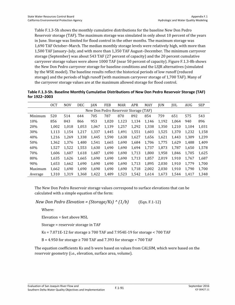
State Water Resources Control Board California Environmental Protection Agency
Appendix F.1 Hydrologic and Water Quality Modeling
Evaluation of San Joaquin River Flow and Southern Delta Water Quality Objectives and Implementation
F.1-91 September 2016
ICF 00427.11
Table F.1.3-5h shows the monthly cumulative distributions for the baseline New Don Pedro
Reservoir storage (TAF). The maximum storage was simulated in only about 10 percent of the years
in June. Storage was limited for flood control in the other months. The maximum storage was
1,690 TAF October–March. The median monthly storage levels were relatively high, with more than
1,500 TAF January–July, and with more than 1,350 TAF August–December. The minimum carryover
storage (September) was about 543 TAF (27 percent of capacity) and the 20 percent cumulative
carryover storage values were above 1000 TAF (near 50 percent of capacity). Figure F.1.3-8b shows
the New Don Pedro carryover storage for baseline conditions and the LSJR alternatives (simulated
by the WSE model). The baseline results reflect the historical periods of low runoff (reduced
storage) and the periods of high runoff (with maximum carryover storage of 1,700 TAF). Many of
the carryover storage values are at the maximum allowed storage for flood control.
Table F.1.3-5h. Baseline Monthly Cumulative Distributions of New Don Pedro Reservoir Storage (TAF) for 1922–2003
OCT NOV DEC JAN FEB MAR APR MAY JUN JUL AUG SEP
New Don Pedro Reservoir Storage (TAF)
Minimum 520 514 644 705 787 870 892 854 759 651 575 543
10% 856 843 866 953 1,020 1,123 1,134 1,146 1,192 1,064 940 896
20% 1,002 1,018 1,053 1,067 1,139 1,257 1,292 1,338 1,350 1,210 1,104 1,031
30% 1,113 1,154 1,217 1,337 1,445 1,491 1,551 1,603 1,525 1,370 1,232 1,158
40% 1,216 1,269 1,338 1,445 1,590 1,638 1,627 1,656 1,621 1,443 1,309 1,239
50% 1,362 1,376 1,480 1,541 1,665 1,690 1,684 1,706 1,775 1,629 1,488 1,409
60% 1,527 1,522 1,553 1,630 1,690 1,690 1,694 1,737 1,873 1,787 1,650 1,578
70% 1,606 1,607 1,618 1,687 1,690 1,690 1,713 1,800 1,958 1,846 1,705 1,625
80% 1,635 1,626 1,665 1,690 1,690 1,690 1,713 1,857 2,019 1,910 1,767 1,687
90% 1,653 1,662 1,690 1,690 1,690 1,690 1,713 1,895 2,030 1,910 1,779 1,700
Maximum 1,662 1,690 1,690 1,690 1,690 1,690 1,718 2,002 2,030 1,910 1,790 1,700
Average 1,310 1,319 1,368 1,422 1,489 1,523 1,542 1,614 1,673 1,544 1,417 1,348
The New Don Pedro Reservoir storage values correspond to surface elevations that can be
calculated with a simple equation of the form:
New Don Pedro Elevation = (Storage/Ks) ^ (1/b) (Eqn. F.1-12)
Where:
Elevation = feet above MSL
Storage = reservoir storage in TAF
Ks = 7.071E-12 for storage ≥ 700 TAF and 7.954E-19 for storage < 700 TAF
B = 4.950 for storage ≥ 700 TAF and 7.393 for storage < 700 TAF
The equation coefficients Ks and b were based on values from CALSIM, which were based on the
reservoir geometry (i.e., elevation, surface area, volume).
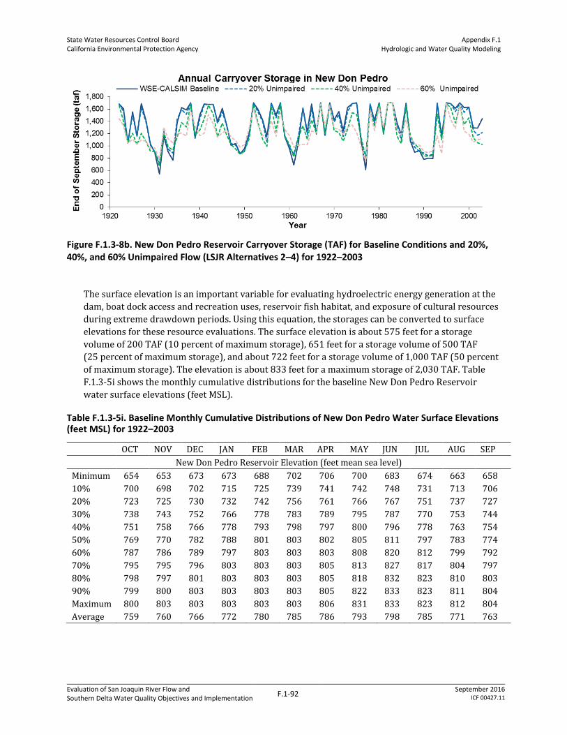
State Water Resources Control Board California Environmental Protection Agency
Appendix F.1 Hydrologic and Water Quality Modeling
Evaluation of San Joaquin River Flow and Southern Delta Water Quality Objectives and Implementation
F.1-92 September 2016
ICF 00427.11
Figure F.1.3-8b. New Don Pedro Reservoir Carryover Storage (TAF) for Baseline Conditions and 20%, 40%, and 60% Unimpaired Flow (LSJR Alternatives 2–4) for 1922–2003
The surface elevation is an important variable for evaluating hydroelectric energy generation at the
dam, boat dock access and recreation uses, reservoir fish habitat, and exposure of cultural resources
during extreme drawdown periods. Using this equation, the storages can be converted to surface
elevations for these resource evaluations. The surface elevation is about 575 feet for a storage
volume of 200 TAF (10 percent of maximum storage), 651 feet for a storage volume of 500 TAF
(25 percent of maximum storage), and about 722 feet for a storage volume of 1,000 TAF (50 percent
of maximum storage). The elevation is about 833 feet for a maximum storage of 2,030 TAF. Table
F.1.3-5i shows the monthly cumulative distributions for the baseline New Don Pedro Reservoir
water surface elevations (feet MSL).
Table F.1.3-5i. Baseline Monthly Cumulative Distributions of New Don Pedro Water Surface Elevations (feet MSL) for 1922–2003
OCT NOV DEC JAN FEB MAR APR MAY JUN JUL AUG SEP
New Don Pedro Reservoir Elevation (feet mean sea level)
Minimum 654 653 673 673 688 702 706 700 683 674 663 658
10% 700 698 702 715 725 739 741 742 748 731 713 706
20% 723 725 730 732 742 756 761 766 767 751 737 727
30% 738 743 752 766 778 783 789 795 787 770 753 744
40% 751 758 766 778 793 798 797 800 796 778 763 754
50% 769 770 782 788 801 803 802 805 811 797 783 774
60% 787 786 789 797 803 803 803 808 820 812 799 792
70% 795 795 796 803 803 803 805 813 827 817 804 797
80% 798 797 801 803 803 803 805 818 832 823 810 803
90% 799 800 803 803 803 803 805 822 833 823 811 804
Maximum 800 803 803 803 803 803 806 831 833 823 812 804
Average 759 760 766 772 780 785 786 793 798 785 771 763
State Water Resources Control Board California Environmental Protection Agency
Appendix F.1 Hydrologic and Water Quality Modeling
Evaluation of San Joaquin River Flow and Southern Delta Water Quality Objectives and Implementation
F.1-93 September 2016
ICF 00427.11
Table F.1.3-5j shows the monthly cumulative distributions for the baseline Tuolumne River target
flows at Modesto. Table F.1.3-5k shows the monthly and annual cumulative distributions for the
baseline Tuolumne River Flows at Modesto. A need for flood control releases is indicated by values
for the cumulative distributions of monthly flows that are higher than the values for the cumulative
distributions of the target flows. Under baseline conditions, flood control releases from New Don
Pedro Reservoir were required in many years, primarily during the late winter and spring. For
example, in April, the average flow was more than 900 cfs greater than the average target flow.
Based on month-by-month comparisons of the Tuolumne River flows at Modesto to the target flows,
about 66 percent of the 82 years modeled required some flood control releases under baseline
conditions.
The median monthly flows were between 422 and 647 cfs in all months, except for March through
May, when median flows were well over 1,000 cfs. The range of annual Tuolumne River flows was
280 TAF (10 percent cumulative) to 1,799 TAF (90 percent cumulative), with a median annual flow
of 572 TAF and an average annual flow of 895 TAF. Figure F.1.3-8c shows the annual sequence of
February–June flows on the Tuolumne River for baseline conditions compared to values for the 20,
40, and 60 percent unimpaired flow simulations.
The baseline Tuolumne River annual diversions (water supply deliveries) ranged from 685 TAF
(10 percent cumulative) to 960 TAF (90 percent cumulative) with a median annual diversion of 878
TAF and an average annual diversion of 851 TAF (Table F.1.3-4b). Figure F.1.3-8d shows the WSE-
simulated sequence of annual Tuolumne River diversions for baseline conditions and the LSJR
alternatives.

State Water Resources Control Board California Environmental Protection Agency
Appendix F.1 Hydrologic and Water Quality Modeling
Evaluation of San Joaquin River Flow and Southern Delta Water Quality Objectives and Implementation
F.1-94 September 2016
ICF 00427.11
Table F.1.3-5j. Baseline Monthly Cumulative Distributions of Target Flows (cfs) for the Tuolumne River at Modesto for 1922–2003
OCT NOV DEC JAN FEB MAR APR MAY JUN JUL AUG SEP
Annual
(TAF)
Tuolumne Target Flow at Modesto (cfs)
Minimum 199 206 71 208 117 — 373 418 193 194 187 166 198
10% 290 246 251 316 276 328 546 540 270 262 277 256 280
20% 395 324 319 417 376 435 665 676 310 319 346 334 343
30% 447 382 399 434 466 476 800 798 368 364 365 366 383
40% 488 443 430 479 487 516 887 1,051 395 403 399 381 415
50% 550 454 445 524 514 573 1,203 1,133 455 448 426 421 431
60% 608 479 496 572 549 606 1,368 1,352 516 519 515 497 465
70% 689 525 581 602 610 652 1,449 1,422 592 568 581 544 518
80% 735 608 602 648 663 702 1,473 1,488 685 601 588 593 546
90% 757 756 655 757 795 782 1,531 1,590 766 681 638 611 594
Maximum 1,171 1,530 1,405 2,411 1,550 1,324 2,108 1,782 1,360 1,067 760 809 815
Average 556 502 479 560 547 573 1,106 1,106 504 471 458 447 441
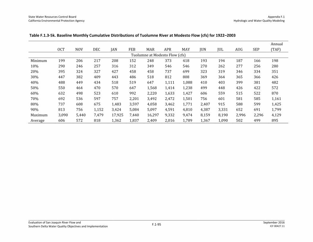
State Water Resources Control Board California Environmental Protection Agency
Appendix F.1 Hydrologic and Water Quality Modeling
Evaluation of San Joaquin River Flow and Southern Delta Water Quality Objectives and Implementation
F.1-95 September 2016
ICF 00427.11
Table F.1.3-5k. Baseline Monthly Cumulative Distributions of Tuolumne River at Modesto Flow (cfs) for 1922–2003
OCT NOV DEC JAN FEB MAR APR MAY JUN JUL AUG SEP
Annual
(TAF)
Tuolumne at Modesto Flow (cfs)
Minimum 199 206 217 208 152 248 373 418 193 194 187 166 198
10% 290 246 257 316 312 349 546 546 270 262 277 256 280
20% 395 324 327 427 458 458 737 699 323 319 346 334 351
30% 447 382 409 443 486 518 812 808 369 364 365 366 426
40% 488 449 434 518 519 647 1,111 1,088 410 403 399 381 482
50% 550 464 470 570 647 1,568 1,414 1,238 499 448 426 422 572
60% 632 498 523 610 992 2,220 1,633 1,427 606 559 515 522 870
70% 692 536 597 757 2,201 3,492 2,472 1,501 756 601 581 585 1,161
80% 737 608 675 1,483 3,597 4,058 3,462 1,771 2,407 915 588 599 1,425
90% 813 756 1,152 3,424 5,084 5,097 4,591 4,810 4,387 3,331 652 691 1,799
Maximum 3,090 5,440 7,479 17,925 7,440 16,297 9,332 9,474 8,159 8,190 2,996 2,296 4,129
Average 606 572 818 1,362 1,837 2,409 2,016 1,789 1,367 1,090 502 499 895

State Water Resources Control Board California Environmental Protection Agency
Appendix F.1 Hydrologic and Water Quality Modeling
Evaluation of San Joaquin River Flow and Southern Delta Water Quality Objectives and Implementation
F.1-96 September 2016
ICF 00427.11
Figure F.1.3-8c. Tuolumne River February–June Flow Volumes (TAF) for Baseline Conditions and 20%, 40%, and 60% Unimpaired Flow (LSJR Alternatives 2–4) for 1922–2003
Figure F.1.3-8d. Tuolumne River Annual Water Supply Diversions for Baseline Conditions and 20%, 40%, and 60% Unimpaired Flow (LSJR Alternatives 2–4) for 1922–2003
Stanislaus River
Figure F.1.3-9a illustrates the basic water supply need for seasonal storage in New Melones
Reservoir to increase the water supply delivery in the summer months when the unimpaired runoff
is less than the monthly demands for irrigation water. Water delivery target was compared to the
distribution of unimpaired flow values, which were shown as 10th, 30th, 50th, 70th, and 90th
percentiles. Because agricultural use requires a specified monthly pattern of water deliveries to
satisfy crop needs (transpiration), storage is needed to extend the period when unimpaired runoff
could be (directly) diverted for irrigation. For the Stanislaus River, the average monthly demands
were less than or equal to the 10 percent cumulative monthly runoff from December through May.
The average June demand was between 30 and 50 percent cumulative runoff, and the average

State Water Resources Control Board California Environmental Protection Agency
Appendix F.1 Hydrologic and Water Quality Modeling
Evaluation of San Joaquin River Flow and Southern Delta Water Quality Objectives and Implementation
F.1-97 September 2016
ICF 00427.11
monthly demands from July through October were greater than the 90 percent cumulative runoff. In
other words, reservoir storage was needed to satisfy the June demand in about 30 to 50 percent of
the years and was needed to satisfy the July–October demands in about 90 percent of the years.
0
50
100
150
200
250
300
350
400
450
500
OCT NOV DEC JAN FEB MAR APR MAY JUN JUL AUG SEP
Flo
w V
olu
me
(TA
F)
Stanislaus Unimpaired Runoff and Diversion Target
10% 30% 50% 70% 90% Diversion Target
Figure F.1.3-9a. Monthly Stanislaus River Unimpaired Runoff Compared to Average Monthly Water Supply Demands
Upstream reservoir operations for seasonal storage and hydroelectric energy generation shift the
monthly inflows to New Melones Reservoir but do not change the annual inflow. Table F.1.3-5l
shows the monthly cumulative distributions for the baseline New Melones storage (TAF). The
maximum storage of 2,420 TAF was simulated in just a few years in June. Storage was limited to less
than 2,000 TAF October–February. The median monthly storage levels were all higher than 1,050
TAF (approximately 44 percent of capacity). The minimum carryover storage (end of September)
was 100 TAF (4 percent of capacity), but the 10 percent cumulative carryover storage was 484 TAF
(approximately 20 percent of capacity). The 50 percent cumulative carryover storage was 1,124 TAF
(46 percent of capacity). Figure F.1.3-9b shows the New Melones carryover storage for baseline
conditions and 20, 40, and 60 percent unimpaired flow. The baseline results reflect the historical
periods of low runoff (reduced storage) and the periods of high runoff (with maximum carryover
storage of 2,000 TAF).
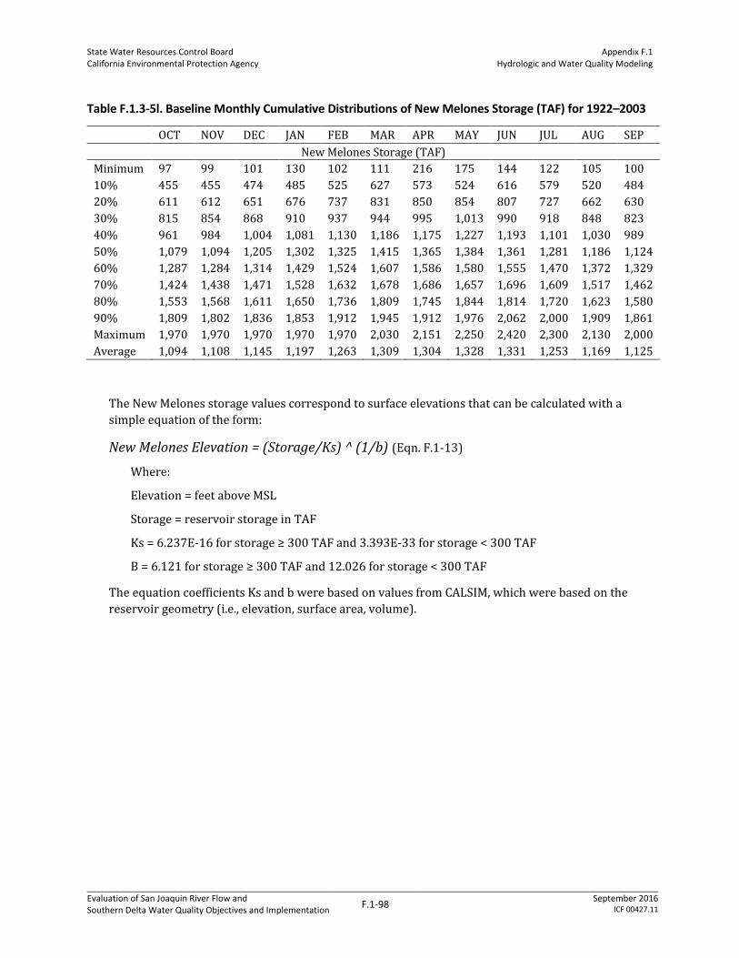
State Water Resources Control Board California Environmental Protection Agency
Appendix F.1 Hydrologic and Water Quality Modeling
Evaluation of San Joaquin River Flow and Southern Delta Water Quality Objectives and Implementation
F.1-98 September 2016
ICF 00427.11
Table F.1.3-5l. Baseline Monthly Cumulative Distributions of New Melones Storage (TAF) for 1922–2003
OCT NOV DEC JAN FEB MAR APR MAY JUN JUL AUG SEP
New Melones Storage (TAF)
Minimum 97 99 101 130 102 111 216 175 144 122 105 100
10% 455 455 474 485 525 627 573 524 616 579 520 484
20% 611 612 651 676 737 831 850 854 807 727 662 630
30% 815 854 868 910 937 944 995 1,013 990 918 848 823
40% 961 984 1,004 1,081 1,130 1,186 1,175 1,227 1,193 1,101 1,030 989
50% 1,079 1,094 1,205 1,302 1,325 1,415 1,365 1,384 1,361 1,281 1,186 1,124
60% 1,287 1,284 1,314 1,429 1,524 1,607 1,586 1,580 1,555 1,470 1,372 1,329
70% 1,424 1,438 1,471 1,528 1,632 1,678 1,686 1,657 1,696 1,609 1,517 1,462
80% 1,553 1,568 1,611 1,650 1,736 1,809 1,745 1,844 1,814 1,720 1,623 1,580
90% 1,809 1,802 1,836 1,853 1,912 1,945 1,912 1,976 2,062 2,000 1,909 1,861
Maximum 1,970 1,970 1,970 1,970 1,970 2,030 2,151 2,250 2,420 2,300 2,130 2,000
Average 1,094 1,108 1,145 1,197 1,263 1,309 1,304 1,328 1,331 1,253 1,169 1,125
The New Melones storage values correspond to surface elevations that can be calculated with a
simple equation of the form:
New Melones Elevation = (Storage/Ks) ^ (1/b) (Eqn. F.1-13)
Where:
Elevation = feet above MSL
Storage = reservoir storage in TAF
Ks = 6.237E-16 for storage ≥ 300 TAF and 3.393E-33 for storage < 300 TAF
B = 6.121 for storage ≥ 300 TAF and 12.026 for storage < 300 TAF
The equation coefficients Ks and b were based on values from CALSIM, which were based on the
reservoir geometry (i.e., elevation, surface area, volume).

State Water Resources Control Board California Environmental Protection Agency
Appendix F.1 Hydrologic and Water Quality Modeling
Evaluation of San Joaquin River Flow and Southern Delta Water Quality Objectives and Implementation
F.1-99 September 2016
ICF 00427.11
Figure F.1.3-9b. New Melones Reservoir Carryover Storage (TAF) for Baseline Conditions and 20%, 40%, and 60% Unimpaired Flow (LSJR Alternatives 2–4) for 1922–2003
The surface elevation is an important variable for evaluating hydroelectric energy generation at the
dam, boat dock access and recreation uses, reservoir fish habitat, and exposure of cultural resources
during extreme drawdown periods. Using this equation, the storages can be converted to surface
elevations for these resource evaluations. The surface elevation was about 793 feet for a storage
volume of 250 TAF (10 percent of maximum storage), 841 feet for a storage volume of 500 TAF
(20 percent of maximum storage), and about 971 feet for a storage volume of 1,200 TAF (50 percent
of maximum storage). The elevation is about 1,089 feet for a maximum storage of 2,420 TAF. Table
F.1.3-5m shows the monthly cumulative distributions for the baseline New Melones Reservoir water
surface elevations (feet).
Table F.1.3-5m. Baseline Monthly Cumulative Distributions of New Melones Water Surface Elevations (feet MSL) for 1922–2003
OCT NOV DEC JAN FEB MAR APR MAY JUN JUL AUG SEP
New Melones Elevation (feet mean sea level)
Minimum 733 735 736 751 736 742 784 770 758 747 738 735
10% 828 828 834 837 848 873 860 848 870 862 847 837
20% 869 870 878 884 897 914 918 918 910 894 881 874
30% 911 918 921 928 932 934 941 944 941 929 917 913
40% 936 940 943 954 961 969 967 974 970 957 947 941
50% 954 956 971 984 987 997 991 994 991 981 969 961
60% 982 982 985 999 1,009 1,018 1,016 1,015 1,013 1,003 992 987
70% 998 1,000 1,004 1,010 1,021 1,025 1,026 1,023 1,027 1,018 1,009 1,003
80% 1,013 1,014 1,019 1,023 1,031 1,038 1,032 1,041 1,039 1,030 1,020 1,015
90% 1,038 1,037 1,041 1,042 1,048 1,051 1,048 1,053 1,061 1,055 1,047 1,043
Maximum 1,053 1,053 1,053 1,053 1,053 1,058 1,068 1,076 1,089 1,080 1,066 1,055
Average 941 943 949 957 965 971 971 974 974 963 952 946

State Water Resources Control Board California Environmental Protection Agency
Appendix F.1 Hydrologic and Water Quality Modeling
Evaluation of San Joaquin River Flow and Southern Delta Water Quality Objectives and Implementation
F.1-100 September 2016
ICF 00427.11
Table F.1.3-5n shows the monthly and annual cumulative distributions for the baseline Stanislaus
River target flows at Ripon, and Table F.1.3-5o shows the monthly and annual cumulative
distributions for the baseline simulated Stanislaus River flows at Ripon. A need for flood control
releases is indicated by values for the cumulative distributions of monthly flows that are higher than
the values for the cumulative distributions of the target flows. Under baseline conditions, flood
control releases from New Melones Reservoir were required less often than were needed on the
Merced or Tuolumne Rivers. Flood control releases were needed more during January and February.
Based on month-by-month comparisons of the Stanislaus River flows at Ripon to the target flows,
about 12 percent of the 82 years modeled required some flood control releases under baseline
conditions.
The median monthly flows were less than 500 cfs July–March, except for October, when required
pulse flows increased the median flow to about 890 cfs. The high April and May flows were the
result of the NMFS BO flow requirements that extend the VAMP flows to a 2-month pulse flow. The
range of annual Stanislaus River flows was 271 TAF (10 percent cumulative) to 786 TAF (90 percent
cumulative), with a median annual flow of 478 TAF and an average annual flow of 549 TAF. Figure
F.1.3-9c shows the annual sequence of February–June flows on the Stanislaus River for baseline
conditions and 20, 40, and 60 percent unimpaired flow.
The baseline Stanislaus River annual diversions (water supply deliveries) ranged from 538 TAF
(10 percent cumulative) to 723 TAF (90 percent cumulative) with a median annual diversion of
661 TAF and an average annual diversion of 637 TAF (Table F.1.3-4a). Figure F.1.3-9d shows the
WSE simulated sequence of annual Stanislaus River diversions for baseline conditions and the LSJR
alternatives.

State Water Resources Control Board California Environmental Protection Agency
Appendix F.1 Hydrologic and Water Quality Modeling
Evaluation of San Joaquin River Flow and Southern Delta Water Quality Objectives and Implementation
F.1-101 September 2016
ICF 00427.11
Table F.1.3-5n. Baseline Monthly Cumulative Distributions of Target Flows (cfs) for the Stanislaus River at Ripon for 1922–2003
OCT NOV DEC JAN FEB MAR APR MAY JUN JUL AUG SEP Annual (TAF)
Stanislaus Target Flow at Ripon (cfs)
Minimum 599 213 — 129 168 58 409 281 210 205 201 174 236
10% 729 248 223 261 230 308 573 525 292 293 302 311 271
20% 772 260 239 294 268 348 765 695 375 324 337 345 336
30% 806 267 262 309 326 372 918 828 444 358 365 369 380
40% 833 292 272 322 368 411 1,177 1,055 536 389 406 397 425
50% 889 319 287 335 384 486 1,556 1,422 629 437 416 419 478
60% 959 337 303 346 401 716 1,674 1,559 1,115 484 455 463 517
70% 979 348 311 366 464 1,265 1,754 1,707 1,276 523 478 490 584
80% 1,041 382 338 407 590 1,672 1,848 1,898 1,427 591 526 520 679
90% 1,110 449 403 506 741 1,842 1,997 2,107 1,625 688 624 666 706
Maximum 1,409 732 674 884 1,465 2,234 2,155 2,603 1,964 1,021 732 887 770
Average 905 328 299 361 453 869 1,347 1,328 872 466 435 448 490

State Water Resources Control Board California Environmental Protection Agency
Appendix F.1 Hydrologic and Water Quality Modeling
Evaluation of San Joaquin River Flow and Southern Delta Water Quality Objectives and Implementation
F.1-102 September 2016
ICF 00427.11
Table F.1.3-5o. Baseline Monthly Cumulative Distributions of Stanislaus River at Ripon Flow (cfs) for 1922–2003
OCT NOV DEC JAN FEB MAR APR MAY JUN JUL AUG SEP Annual (TAF)
Stanislaus at Ripon Flow (cfs)
Minimum 599 213 — 198 168 58 409 281 210 205 201 174 236
10% 729 248 224 270 230 308 573 525 292 293 302 311 271
20% 772 260 241 295 268 348 765 695 375 324 337 345 336
30% 806 267 262 312 326 372 918 828 444 358 365 369 380
40% 833 292 280 324 368 411 1,177 1,055 536 389 406 397 425
50% 889 319 288 337 385 486 1,556 1,422 629 437 416 419 478
60% 959 337 304 349 415 716 1,674 1,559 1,115 484 463 463 517
70% 979 348 316 375 507 1,265 1,754 1,707 1,281 531 483 490 584
80% 1,042 382 348 449 654 1,717 1,848 1,898 1,456 616 529 528 681
90% 1,116 454 421 576 1,285 1,911 1,997 2,107 1,655 705 632 667 786
Maximum 1,810 3,453 5,126 10,555 5,177 6,223 2,155 2,603 4,653 4,340 2,664 3,050 2,520
Average 919 394 398 644 655 960 1,347 1,328 913 522 483 521 549

State Water Resources Control Board California Environmental Protection Agency
Appendix F.1 Hydrologic and Water Quality Modeling
Evaluation of San Joaquin River Flow and Southern Delta Water Quality Objectives and Implementation
F.1-103 September 2016
ICF 00427.11
Figure F.1.3-9c. Stanislaus River February–June Flow Volumes (TAF) for Baseline Conditions and 20%, 40%, and 60% Unimpaired Flow (LSJR Alternatives 2–4) for 1922–2003
Figure F.1.3-9d. Stanislaus River Annual Water Supply Diversions for Baseline Conditions and 20%, 40%, and 60% Unimpaired Flow (LSJR Alternatives 2–4) for 1922–2003
SJR at Vernalis
Table F.1.3-5p shows the monthly and annual cumulative distributions for the baseline SJR flows at
Vernalis, downstream of the Stanislaus River. The median monthly baseline flows were between
1,500 and 2,600 cfs from June to January and 3,400 and 4,700 cfs from February to May. The higher
median flows in April and May were caused by the Vernalis pulse flows. High flows, greater than
10,000 cfs from January to June (i.e., reservoir flood control releases), were simulated in only about
10 percent of the years. The range of annual SJR flows was 1,077 TAF (10 percent cumulative) to
5,542 TAF (90 percent cumulative), with a median annual flow of 2,041 TAF and an average annual
flow of 2,965 TAF. Figure F.1.3-10 shows the annual sequence of February to June flows on the SJR
at Vernalis for baseline conditions and 20, 40, and 60 percent unimpaired flows.
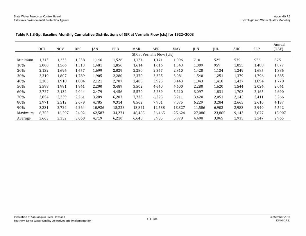
State Water Resources Control Board California Environmental Protection Agency
Appendix F.1 Hydrologic and Water Quality Modeling
Evaluation of San Joaquin River Flow and Southern Delta Water Quality Objectives and Implementation
F.1-104 September 2016
ICF 00427.11
Table F.1.3-5p. Baseline Monthly Cumulative Distributions of SJR at Vernalis Flow (cfs) for 1922–2003
OCT NOV DEC JAN FEB MAR APR MAY JUN JUL AUG SEP Annual (TAF)
SJR at Vernalis Flow (cfs)
Minimum 1,343 1,233 1,238 1,146 1,526 1,124 1,171 1,096 710 525 579 955 875
10% 2,000 1,566 1,513 1,481 1,856 1,614 1,616 1,543 1,009 959 1,055 1,488 1,077
20% 2,132 1,696 1,657 1,699 2,029 2,280 2,347 2,310 1,420 1,134 1,249 1,685 1,386
30% 2,319 1,807 1,789 1,905 2,280 2,370 3,325 3,081 1,540 1,251 1,379 1,796 1,585
40% 2,385 1,918 1,884 2,121 2,707 3,405 3,925 3,443 1,843 1,418 1,437 1,894 1,778
50% 2,598 1,981 1,941 2,200 3,489 3,502 4,640 4,600 2,280 1,620 1,544 2,024 2,041
60% 2,727 2,132 2,044 2,479 4,456 5,570 5,239 5,210 3,097 1,831 1,703 2,165 2,690
70% 2,854 2,239 2,261 3,289 6,207 7,733 6,225 5,211 3,420 2,051 2,142 2,411 3,266
80% 2,971 2,512 2,679 4,785 9,314 8,562 7,901 7,075 6,229 3,284 2,665 2,610 4,197
90% 3,331 2,724 4,264 10,926 15,228 13,821 12,538 13,327 11,586 6,902 2,983 2,940 5,542
Maximum 6,753 16,297 24,021 62,587 34,271 48,485 26,465 25,624 27,086 23,865 9,143 7,677 15,907
Average 2,663 2,352 3,060 4,719 6,210 6,640 5,985 5,978 4,408 3,065 1,935 2,247 2,965

State Water Resources Control Board California Environmental Protection Agency
Appendix F.1 Hydrologic and Water Quality Modeling
Evaluation of San Joaquin River Flow and Southern Delta Water Quality Objectives and Implementation
F.1-105 September 2016
ICF 00427.11
Figure F.1.3-10. SJR at Vernalis February–June Flow Volumes for Baseline Conditions and 20%, 40%, and 60% Unimpaired Flow (LSJR Alternatives 2–4) for 1922–2003
F.1.3.3 20 Percent Unimpaired Flow (LSJR Alternative 2)
The WSE model was used to simulate 20 percent unimpaired flow, which represents typical
conditions for LSJR Alternative 2. For this simulation, LSJR tributary flows were greater than or
equal to 20 percent of the unimpaired flow for February–June. In some years February–June flows
were higher than the 20 percent unimpaired flow objective because of flood control releases or
other flow requirements. The reservoir storage and water supply diversions were adjusted to satisfy
these monthly flow objectives for each of the eastside tributaries. Flood control releases were
reduced or eliminated in some years because more water was released to satisfy the flow objectives.
Water supply diversions were reduced in some years to account for the 20 percent unimpaired flow
requirement and maintain storage in the reservoirs.
Merced River
Table F.1.3-6a shows the monthly cumulative distributions for the WSE-calculated Lake McClure
storage (TAF) for LSJR Alternative 2. These monthly storage patterns differ from baseline storage
patterns because the timing and magnitude of releases for instream flow requirements and
diversions are different. The median carryover storage was 499 TAF, slightly higher than the
baseline median carryover storage of 451 TAF. Table F.1.3-6b shows the monthly cumulative
distributions for the WSE-calculated Lake McClure water surface elevations (feet MSL) for LSJR
Alternative 2. The median September reservoir elevation was 770 TAF, slightly higher than the
baseline median September elevation of 757 TAF.

State Water Resources Control Board California Environmental Protection Agency
Appendix F.1 Hydrologic and Water Quality Modeling
Evaluation of San Joaquin River Flow and Southern Delta Water Quality Objectives and Implementation
F.1-106 September 2016
ICF 00427.11
Table F.1.3-6a. WSE Results for Lake McClure Storage (TAF) for 20% Unimpaired Flow (LSJR Alternative 2)
OCT NOV DEC JAN FEB MAR APR MAY JUN JUL AUG SEP
Lake McClure Storage (TAF)
Min 165 148 165 229 214 193 204 211 225 245 216 194
10% 274 264 261 265 302 319 351 413 416 367 326 302
20% 293 289 319 329 375 382 415 486 493 439 371 325
30% 366 361 367 392 445 488 558 599 577 494 429 395
40% 385 390 425 478 553 619 647 699 657 547 451 411
50% 471 465 519 587 637 659 686 729 737 652 554 499
60% 593 596 616 636 674 687 742 851 858 766 670 618
70% 657 644 650 669 675 723 774 922 963 883 770 700
80% 668 662 668 675 675 735 818 966 1,024 910 770 700
90% 675 675 675 675 675 735 845 970 1,024 910 770 700
Max 675 675 675 675 675 735 845 970 1,024 910 770 700
Avg 482 480 493 515 546 581 639 727 741 655 561 511
Table F.1.3-6b. WSE Results for Lake McClure Water Surface Elevations (feet MSL) for 20% Unimpaired Flow (20% Unimpaired Flow)
OCT NOV DEC JAN FEB MAR APR MAY JUN JUL AUG SEP
Lake McClure Elevation (feet mean sea level)
Minimum 659 650 659 685 682 672 677 680 686 685 682 673
10% 698 693 692 694 709 715 727 746 747 732 718 709
20% 705 704 715 719 735 737 747 767 769 754 733 717
30% 732 730 732 740 756 767 784 794 789 769 751 741
40% 738 739 750 765 783 798 804 814 806 782 757 746
50% 763 761 775 791 802 806 812 820 821 805 784 770
60% 792 793 797 802 809 812 822 841 842 826 809 798
70% 806 803 804 808 809 819 828 852 858 846 827 814
80% 808 807 808 809 809 821 836 859 867 850 827 814
90% 809 809 809 809 809 821 840 859 867 850 827 814
Maximum 809 809 809 809 809 821 840 859 867 850 827 814
Average 759 759 762 768 776 784 796 813 815 799 779 767
Table F.1.3-6c shows the monthly cumulative distributions for the WSE-calculated Merced River
target flows at Stevinson for 20 percent unimpaired flow. Target flows are the flows specified for the
downstream ends of the river in the absence of flood control releases. Comparison to the baseline
indicates that the average monthly target flows for LSJR Alternative 2 increased from February–June
and remained unchanged from July–January. The greatest increase came in May when the average
target flow increased from 341 cfs under baseline to 785 cfs under the alternative.

State Water Resources Control Board California Environmental Protection Agency
Appendix F.1 Hydrologic and Water Quality Modeling
Evaluation of San Joaquin River Flow and Southern Delta Water Quality Objectives and Implementation
F.1-107 September 2016
ICF 00427.11
Table F.1.3-6c. Merced River Target Flows (cfs) for 20% Unimpaired Flow (LSJR Alternative 2)
OCT NOV DEC JAN FEB MAR APR MAY JUN JUL AUG SEP
Merced Target Flow (cfs)
Minimum (0) 152 33 99 207 205 186 182 44 (0) (0) (0)
10% 300 255 263 260 306 297 283 330 171 47 19 36
20% 350 290 287 318 336 335 317 435 229 82 56 67
30% 372 312 309 332 353 355 378 566 276 101 84 87
40% 393 325 332 345 385 372 432 658 383 132 110 118
50% 414 336 338 360 397 398 477 792 491 147 122 131
60% 430 346 352 386 449 475 533 876 562 174 144 146
70% 450 353 363 424 545 504 576 946 691 223 171 167
80% 462 369 381 482 660 575 647 1,045 881 240 196 192
90% 502 396 409 560 828 672 735 1,261 1,127 276 220 222
Maximum 1,276 847 1,075 1,730 2,059 2,037 1,442 1,838 2,205 1,133 536 629
Average 415 338 344 416 513 478 510 785 583 175 128 135
Table F.1.3-6d shows the monthly cumulative distributions for the WSE-calculated Merced River
flows at Stevinson for LSJR Alternative 2. The Merced River flows were changed mostly in the
February–June period. The monthly flows were higher than the target flows for the higher
cumulative distribution values, indicating that flood control releases were required for LSJR
Alternative 2 in many years, particularly during February. Based on month-by-month comparisons
of the Merced River flows at Stevinson to the target flows, about 51 percent of the 82 years modeled
required some flood control releases.

State Water Resources Control Board California Environmental Protection Agency
Appendix F.1 Hydrologic and Water Quality Modeling
Evaluation of San Joaquin River Flow and Southern Delta Water Quality Objectives and Implementation
F.1-108 September 2016
ICF 00427.11
Table F.1.3-6d. Merced River Flows at Stevinson (cfs) for 20% Unimpaired Flow (LSJR Alternative 2)
OCT NOV DEC JAN FEB MAR APR MAY JUN JUL AUG SEP Annual (TAF)
Merced at Stevinson Flow (cfs)
Minimum 219 208 83 144 207 205 186 182 44 (0) (0) (0) 165
10% 325 271 281 280 312 297 283 330 171 55 30 53 187
20% 356 300 306 327 337 335 317 435 229 90 72 89 216
30% 380 318 325 342 372 355 378 566 276 113 104 120 241
40% 399 332 337 358 396 372 432 658 383 138 122 137 261
50% 423 340 349 378 470 399 477 792 491 153 155 166 293
60% 440 350 359 422 662 485 536 890 562 202 199 196 366
70% 457 361 374 528 843 550 578 946 698 232 401 332 536
80% 473 376 409 1,012 1,653 969 665 1,175 1,596 993 971 420 765
90% 563 437 1,037 1,725 2,874 1,728 914 2,445 2,658 2,113 1,159 545 1,016
Maximum 1,276 1,910 3,495 9,859 5,092 5,959 4,845 5,379 7,273 5,863 2,392 1,275 2,398
Average 440 395 540 835 1,074 813 603 1,020 1,011 644 414 260 485
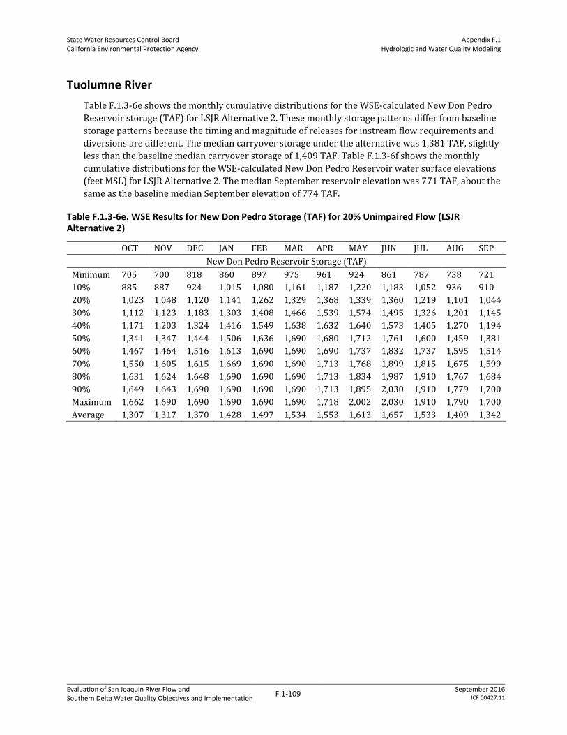
State Water Resources Control Board California Environmental Protection Agency
Appendix F.1 Hydrologic and Water Quality Modeling
Evaluation of San Joaquin River Flow and Southern Delta Water Quality Objectives and Implementation
F.1-109 September 2016
ICF 00427.11
Tuolumne River
Table F.1.3-6e shows the monthly cumulative distributions for the WSE-calculated New Don Pedro
Reservoir storage (TAF) for LSJR Alternative 2. These monthly storage patterns differ from baseline
storage patterns because the timing and magnitude of releases for instream flow requirements and
diversions are different. The median carryover storage under the alternative was 1,381 TAF, slightly
less than the baseline median carryover storage of 1,409 TAF. Table F.1.3-6f shows the monthly
cumulative distributions for the WSE-calculated New Don Pedro Reservoir water surface elevations
(feet MSL) for LSJR Alternative 2. The median September reservoir elevation was 771 TAF, about the
same as the baseline median September elevation of 774 TAF.
Table F.1.3-6e. WSE Results for New Don Pedro Storage (TAF) for 20% Unimpaired Flow (LSJR Alternative 2)
OCT NOV DEC JAN FEB MAR APR MAY JUN JUL AUG SEP
New Don Pedro Reservoir Storage (TAF)
Minimum 705 700 818 860 897 975 961 924 861 787 738 721
10% 885 887 924 1,015 1,080 1,161 1,187 1,220 1,183 1,052 936 910
20% 1,023 1,048 1,120 1,141 1,262 1,329 1,368 1,339 1,360 1,219 1,101 1,044
30% 1,112 1,123 1,183 1,303 1,408 1,466 1,539 1,574 1,495 1,326 1,201 1,145
40% 1,171 1,203 1,324 1,416 1,549 1,638 1,632 1,640 1,573 1,405 1,270 1,194
50% 1,341 1,347 1,444 1,506 1,636 1,690 1,680 1,712 1,761 1,600 1,459 1,381
60% 1,467 1,464 1,516 1,613 1,690 1,690 1,690 1,737 1,832 1,737 1,595 1,514
70% 1,550 1,605 1,615 1,669 1,690 1,690 1,713 1,768 1,899 1,815 1,675 1,599
80% 1,631 1,624 1,648 1,690 1,690 1,690 1,713 1,834 1,987 1,910 1,767 1,684
90% 1,649 1,643 1,690 1,690 1,690 1,690 1,713 1,895 2,030 1,910 1,779 1,700
Maximum 1,662 1,690 1,690 1,690 1,690 1,690 1,718 2,002 2,030 1,910 1,790 1,700
Average 1,307 1,317 1,370 1,428 1,497 1,534 1,553 1,613 1,657 1,533 1,409 1,342

State Water Resources Control Board California Environmental Protection Agency
Appendix F.1 Hydrologic and Water Quality Modeling
Evaluation of San Joaquin River Flow and Southern Delta Water Quality Objectives and Implementation
F.1-110 September 2016
ICF 00427.11
Table F.1.3-6f. WSE Results for New Don Pedro Water Surface Elevations (feet MSL) for 20% Unimpaired Flow (LSJR Alternative 2)
OCT NOV DEC JAN FEB MAR APR MAY JUN JUL AUG SEP
New Don Pedro Reservoir Elevation (feet mean sea level)
Minimum 673 672 694 701 707 719 716 711 701 688 679 676
10% 705 705 711 724 734 744 748 752 747 730 713 709
20% 726 729 739 742 757 765 770 766 769 752 736 729
30% 738 739 747 762 774 780 788 792 783 765 749 742
40% 746 750 764 775 789 798 797 798 792 774 758 749
50% 766 767 778 785 798 803 802 805 810 794 780 771
60% 780 780 786 796 803 803 803 807 816 807 794 785
70% 789 795 796 801 803 803 805 810 822 815 802 794
80% 797 797 799 803 803 803 805 816 830 823 810 802
90% 799 798 803 803 803 803 805 822 833 823 811 804
Maximum 800 803 803 803 803 803 806 831 833 823 812 804
Average 759 760 767 774 782 786 788 794 797 784 771 763
Table F.1.3-6g shows the monthly cumulative distributions for the WSE-calculated Tuolumne River
target flows at Modesto for LSJR Alternative 2. Target flows are the flows specified for the
downstream ends of the river in the absence of flood control releases. Comparison to the baseline
indicates that the average monthly target flows for LSJR Alternative 2 increased from February–June
and remain unchanged from July–January. The greatest increase came in June when the average
target flow increased from 504 cfs under baseline to 1,203 cfs under the alternative.

State Water Resources Control Board California Environmental Protection Agency
Appendix F.1 Hydrologic and Water Quality Modeling
Evaluation of San Joaquin River Flow and Southern Delta Water Quality Objectives and Implementation
F.1-111 September 2016
ICF 00427.11
Table F.1.3-6g. Tuolumne River Target Flows (cfs) for 20% Unimpaired Flow (LSJR Alternative 2)
OCT NOV DEC JAN FEB MAR APR MAY JUN JUL AUG SEP
Tuolumne Target Flow (cfs)
Minimum 199 206 71 208 235 338 411 418 283 194 187 166
10% 290 246 251 316 348 434 633 695 374 262 277 256
20% 395 324 319 417 466 486 783 977 457 319 346 334
30% 447 382 399 434 487 538 852 1,124 742 364 365 366
40% 488 443 430 479 524 595 1,042 1,232 969 403 399 381
50% 550 454 445 524 580 628 1,207 1,469 1,129 448 426 421
60% 608 479 496 572 617 686 1,353 1,666 1,343 519 515 497
70% 689 525 581 602 795 738 1,417 1,752 1,495 568 581 544
80% 735 608 602 648 934 853 1,469 1,870 1,785 601 588 593
90% 757 756 655 757 1,158 1,115 1,525 2,142 2,009 681 638 611
Maximum 1,171 1,530 1,405 2,411 2,218 1,883 2,218 3,123 3,415 1,067 760 809
Average 556 502 479 560 680 711 1,158 1,460 1,203 471 458 447
Table F.1.3-6h shows the monthly cumulative distributions for the WSE-calculated Tuolumne River
flows at Modesto for LSJR Alternative 2. The Tuolumne River flows were generally changed only in
the February–June period. The cumulative distributions of monthly flows were often higher than the
cumulative distributions of the target flows, indicating that flood control releases were required in
many years, particularly in February through April. Based on month-by-month comparisons of the
Tuolumne River flows at Modesto to the target flows, about 63 percent of the 82 years modeled
required some flood control releases.
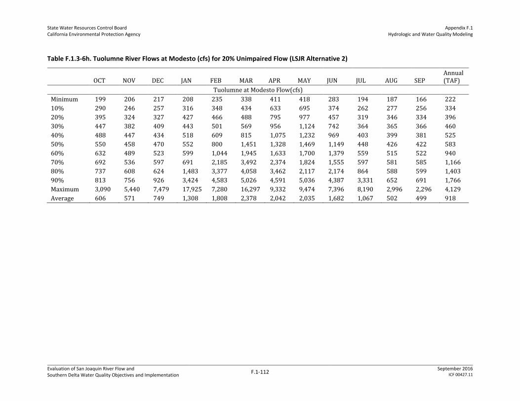
State Water Resources Control Board California Environmental Protection Agency
Appendix F.1 Hydrologic and Water Quality Modeling
Evaluation of San Joaquin River Flow and Southern Delta Water Quality Objectives and Implementation
F.1-112 September 2016
ICF 00427.11
Table F.1.3-6h. Tuolumne River Flows at Modesto (cfs) for 20% Unimpaired Flow (LSJR Alternative 2)
OCT NOV DEC JAN FEB MAR APR MAY JUN JUL AUG SEP Annual (TAF)
Tuolumne at Modesto Flow(cfs)
Minimum 199 206 217 208 235 338 411 418 283 194 187 166 222
10% 290 246 257 316 348 434 633 695 374 262 277 256 334
20% 395 324 327 427 466 488 795 977 457 319 346 334 396
30% 447 382 409 443 501 569 956 1,124 742 364 365 366 460
40% 488 447 434 518 609 815 1,075 1,232 969 403 399 381 525
50% 550 458 470 552 800 1,451 1,328 1,469 1,149 448 426 422 583
60% 632 489 523 599 1,044 1,945 1,633 1,700 1,379 559 515 522 940
70% 692 536 597 691 2,185 3,492 2,374 1,824 1,555 597 581 585 1,166
80% 737 608 624 1,483 3,377 4,058 3,462 2,117 2,174 864 588 599 1,403
90% 813 756 926 3,424 4,583 5,026 4,591 5,036 4,387 3,331 652 691 1,766
Maximum 3,090 5,440 7,479 17,925 7,280 16,297 9,332 9,474 7,396 8,190 2,996 2,296 4,129
Average 606 571 749 1,308 1,808 2,378 2,042 2,035 1,682 1,067 502 499 918
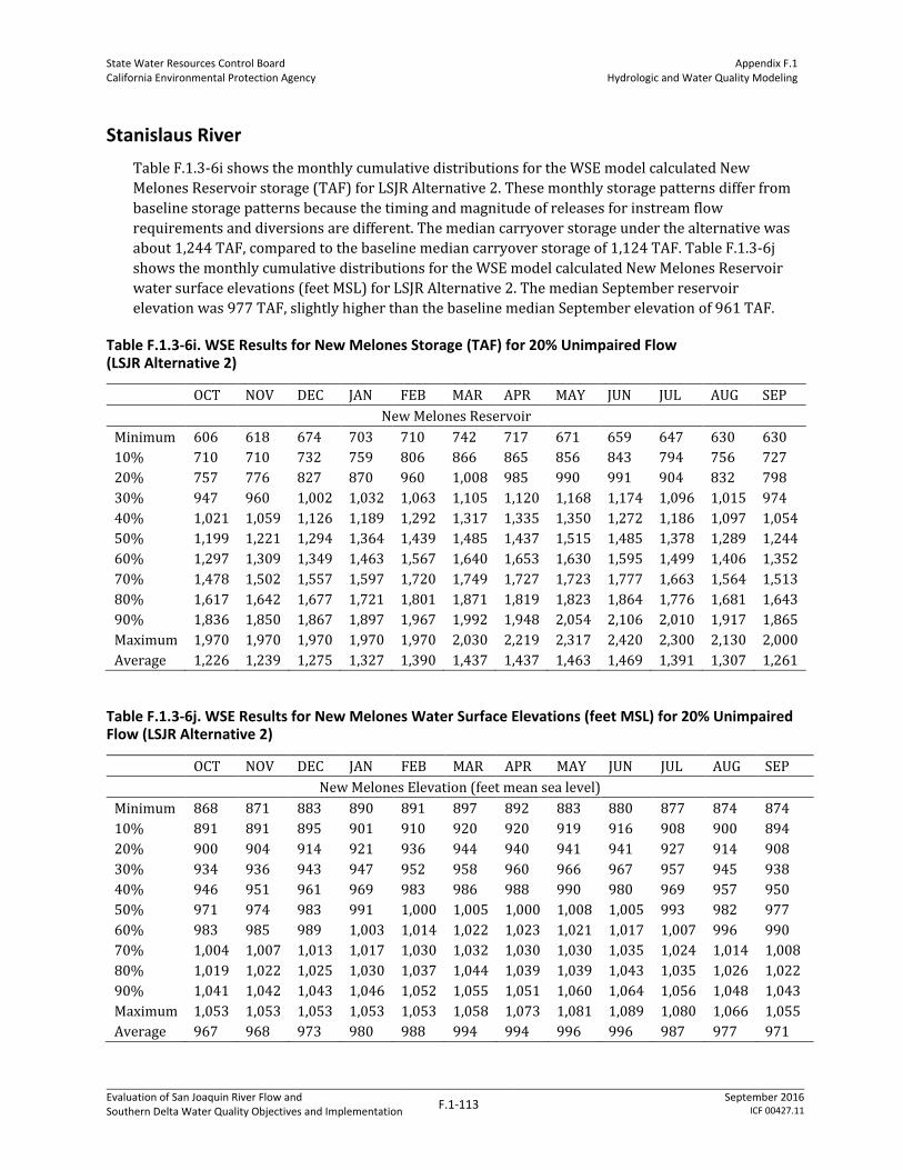
State Water Resources Control Board California Environmental Protection Agency
Appendix F.1 Hydrologic and Water Quality Modeling
Evaluation of San Joaquin River Flow and Southern Delta Water Quality Objectives and Implementation
F.1-113 September 2016
ICF 00427.11
Stanislaus River
Table F.1.3-6i shows the monthly cumulative distributions for the WSE model calculated New
Melones Reservoir storage (TAF) for LSJR Alternative 2. These monthly storage patterns differ from
baseline storage patterns because the timing and magnitude of releases for instream flow
requirements and diversions are different. The median carryover storage under the alternative was
about 1,244 TAF, compared to the baseline median carryover storage of 1,124 TAF. Table F.1.3-6j
shows the monthly cumulative distributions for the WSE model calculated New Melones Reservoir
water surface elevations (feet MSL) for LSJR Alternative 2. The median September reservoir
elevation was 977 TAF, slightly higher than the baseline median September elevation of 961 TAF.
Table F.1.3-6i. WSE Results for New Melones Storage (TAF) for 20% Unimpaired Flow (LSJR Alternative 2)
OCT NOV DEC JAN FEB MAR APR MAY JUN JUL AUG SEP
New Melones Reservoir
Minimum 606 618 674 703 710 742 717 671 659 647 630 630
10% 710 710 732 759 806 866 865 856 843 794 756 727
20% 757 776 827 870 960 1,008 985 990 991 904 832 798
30% 947 960 1,002 1,032 1,063 1,105 1,120 1,168 1,174 1,096 1,015 974
40% 1,021 1,059 1,126 1,189 1,292 1,317 1,335 1,350 1,272 1,186 1,097 1,054
50% 1,199 1,221 1,294 1,364 1,439 1,485 1,437 1,515 1,485 1,378 1,289 1,244
60% 1,297 1,309 1,349 1,463 1,567 1,640 1,653 1,630 1,595 1,499 1,406 1,352
70% 1,478 1,502 1,557 1,597 1,720 1,749 1,727 1,723 1,777 1,663 1,564 1,513
80% 1,617 1,642 1,677 1,721 1,801 1,871 1,819 1,823 1,864 1,776 1,681 1,643
90% 1,836 1,850 1,867 1,897 1,967 1,992 1,948 2,054 2,106 2,010 1,917 1,865
Maximum 1,970 1,970 1,970 1,970 1,970 2,030 2,219 2,317 2,420 2,300 2,130 2,000
Average 1,226 1,239 1,275 1,327 1,390 1,437 1,437 1,463 1,469 1,391 1,307 1,261
Table F.1.3-6j. WSE Results for New Melones Water Surface Elevations (feet MSL) for 20% Unimpaired Flow (LSJR Alternative 2)
OCT NOV DEC JAN FEB MAR APR MAY JUN JUL AUG SEP
New Melones Elevation (feet mean sea level)
Minimum 868 871 883 890 891 897 892 883 880 877 874 874
10% 891 891 895 901 910 920 920 919 916 908 900 894
20% 900 904 914 921 936 944 940 941 941 927 914 908
30% 934 936 943 947 952 958 960 966 967 957 945 938
40% 946 951 961 969 983 986 988 990 980 969 957 950
50% 971 974 983 991 1,000 1,005 1,000 1,008 1,005 993 982 977
60% 983 985 989 1,003 1,014 1,022 1,023 1,021 1,017 1,007 996 990
70% 1,004 1,007 1,013 1,017 1,030 1,032 1,030 1,030 1,035 1,024 1,014 1,008
80% 1,019 1,022 1,025 1,030 1,037 1,044 1,039 1,039 1,043 1,035 1,026 1,022
90% 1,041 1,042 1,043 1,046 1,052 1,055 1,051 1,060 1,064 1,056 1,048 1,043
Maximum 1,053 1,053 1,053 1,053 1,053 1,058 1,073 1,081 1,089 1,080 1,066 1,055
Average 967 968 973 980 988 994 994 996 996 987 977 971

State Water Resources Control Board California Environmental Protection Agency
Appendix F.1 Hydrologic and Water Quality Modeling
Evaluation of San Joaquin River Flow and Southern Delta Water Quality Objectives and Implementation
F.1-114 September 2016
ICF 00427.11
Table F.1.3-6k shows the monthly cumulative distributions for the WSE-calculated Stanislaus River
target flows at Ripon for LSJR Alternative 2. Target flows are the flows specified for the downstream
ends of the river in the absence of flood control releases. The average monthly target flows under
LSJR Alternative 2 were similar to the flows under baseline conditions, with slight differences
because of changes in the NMI under the alternative. From March to June, the average monthly
target flows were generally lower than the baseline targets. These target flows were reduced as a
result of removing the Vernalis D1641 minimum flow requirements and the VAMP requirements.
Table F.1.3-6k. Stanislaus River Target Flows (cfs) for 20% Unimpaired Flow (LSJR Alternative 2)
OCT NOV DEC JAN FEB MAR APR MAY JUN JUL AUG SEP
Stanislaus Target Flow (cfs)
Minimum 599 213 94 129 216 238 393 299 188 205 208 174
10% 760 248 223 261 239 313 600 553 316 297 312 312
20% 774 260 241 294 308 340 798 726 363 325 352 358
30% 827 267 262 312 355 370 908 942 500 364 381 387
40% 850 292 273 325 373 384 1,122 1,263 587 395 413 419
50% 902 318 288 339 389 415 1,495 1,373 778 437 424 429
60% 970 336 304 349 422 497 1,650 1,478 836 500 463 469
70% 979 348 316 366 482 1,604 1,744 1,670 1,135 538 478 497
80% 1,041 382 347 407 600 1,719 1,775 1,743 1,281 618 538 537
90% 1,109 453 403 506 823 1,897 1,858 2,036 1,544 688 625 666
Maximum 1,409 732 674 884 1,916 2,234 2,088 2,425 2,124 1,021 732 887
Average 913 330 303 361 479 860 1,314 1,318 848 475 443 456
Table F.1.3-6l shows the monthly cumulative distributions for the Stanislaus River flows at Ripon for
LSJR Alternative 2. The Stanislaus River flows were generally changed only in the February–June
period. The cumulative distributions of the monthly flows were occasionally higher than the target
flows, indicating that flood control releases were sometimes required. Based on month-by-month
comparisons of the Stanislaus River flows at Ripon to the target flows, about 18 percent of the
82 years modeled required some flood control releases (less often than was needed on the Merced
or Tuolumne Rivers).

State Water Resources Control Board California Environmental Protection Agency
Appendix F.1 Hydrologic and Water Quality Modeling
Evaluation of San Joaquin River Flow and Southern Delta Water Quality Objectives and Implementation
F.1-115 September 2016
ICF 00427.11
Table F.1.3-6l. Stanislaus River Flows at Ripon (cfs) for 20% Unimpaired Flow (LSJR Alternative 2)
OCT NOV DEC JAN FEB MAR APR MAY JUN JUL AUG SEP Annual (TAF)
Stanislaus at Ripon Flow (cfs)
Minimum 599 213 94 198 216 238 393 299 188 205 208 174 241
10% 760 248 225 270 239 313 600 553 316 297 312 312 284
20% 774 260 242 295 308 340 798 726 363 325 352 358 339
30% 827 267 262 317 355 370 908 942 500 364 381 387 369
40% 850 292 280 327 376 384 1,122 1,263 587 395 413 419 422
50% 902 318 291 343 389 415 1,495 1,373 778 437 424 429 474
60% 970 336 305 352 437 497 1,650 1,478 836 510 463 469 505
70% 979 348 320 375 546 1,639 1,744 1,670 1,135 540 483 501 624
80% 1,042 382 368 446 657 1,776 1,775 1,743 1,281 627 541 564 694
90% 1,128 456 423 606 1,315 1,911 1,858 2,036 1,544 726 632 689 929
Maximum 1,810 3,453 5,126 10,555 5,177 6,223 2,088 2,425 4,653 4,340 2,664 3,050 2,520
Average 928 395 426 645 696 949 1,314 1,318 878 537 521 564 554

State Water Resources Control Board California Environmental Protection Agency
Appendix F.1 Hydrologic and Water Quality Modeling
Evaluation of San Joaquin River Flow and Southern Delta Water Quality Objectives and Implementation
F.1-116 September 2016
ICF 00427.11
SJR at Vernalis
Table F.1.3-6m shows the monthly cumulative distributions for the WSE-calculated SJR at Vernalis
flows for LSJR Alternative 2. The SJR at Vernalis flows changed most during May and June. LSJR
Alternative 2 provided a more natural distribution of flows from February–June. The average annual
flow was about 59 TAF more (2 percent) than the average baseline flow.

State Water Resources Control Board California Environmental Protection Agency
Appendix F.1 Hydrologic and Water Quality Modeling
Evaluation of San Joaquin River Flow and Southern Delta Water Quality Objectives and Implementation
F.1-117 September 2016
ICF 00427.11
Table F.1.3-6m. SJR Flows at Vernalis (cfs) for 20% Unimpaired Flow (LSJR Alternative 2)
OCT NOV DEC JAN FEB MAR APR MAY JUN JUL AUG SEP Annual (TAF)
SJR at Vernalis Flow (cfs)
Minimum 1,343 1,233 1,238 1,146 1,526 1,124 1,349 1,267 1,000 525 579 955 915
10% 2,000 1,566 1,513 1,481 1,775 1,617 1,867 2,202 1,114 959 1,055 1,488 1,136
20% 2,147 1,696 1,657 1,699 1,937 1,810 2,499 2,930 1,540 1,139 1,249 1,685 1,451
30% 2,335 1,807 1,789 1,886 2,223 2,467 3,125 3,361 1,894 1,251 1,379 1,796 1,594
40% 2,395 1,918 1,884 2,121 2,445 2,979 3,603 4,203 2,583 1,447 1,449 1,913 1,825
50% 2,611 1,981 1,941 2,225 3,623 3,606 4,280 4,522 3,334 1,639 1,565 2,024 2,102
60% 2,755 2,132 2,035 2,373 4,575 5,295 5,074 5,522 3,719 1,819 1,682 2,173 2,740
70% 2,889 2,266 2,240 3,153 6,321 7,748 6,032 6,071 3,993 2,034 2,112 2,416 3,269
80% 2,992 2,525 2,622 4,849 9,115 9,231 8,229 8,106 6,093 3,284 2,718 2,616 4,507
90% 3,331 2,777 3,885 11,153 14,905 13,821 13,179 14,366 11,700 6,902 3,029 3,216 5,505
Maximum 6,753 16,297 24,021 62,587 34,271 48,485 26,465 25,624 27,086 23,865 9,143 7,677 15,907
Average 2,673 2,363 3,041 4,721 6,237 6,624 5,992 6,446 4,840 3,041 1,967 2,289 3,024

State Water Resources Control Board California Environmental Protection Agency
Appendix F.1 Hydrologic and Water Quality Modeling
Evaluation of San Joaquin River Flow and Southern Delta Water Quality Objectives and Implementation
F.1-118 September 2016
ICF 00427.11
F.1.3.4 40 Percent Unimpaired Flow (LSJR Alternative 3)
The WSE model was used to simulate 40 percent unimpaired flow, which represents typical
conditions for LSJR Alternative 3. For this simulation, LSJR tributary flows were generally greater
than or equal to 40 percent of the unimpaired flow from February–June. Some of the February–June
flow was reserved for controlling potential temperature effects later in the year; thus, resulting
flows decreased to slightly below 40 percent of unimpaired flow during some years. In some years,
February–June flows were higher than the 40 percent unimpaired flow objective because of flood
control releases or other flow requirements. The reservoir storage and water supply diversions
were managed to satisfy these monthly flow objectives for each tributary river. Flood releases in
many years were reduced or eliminated because higher flows were released from February–June to
satisfy the flow objectives. Water supply diversions were reduced in some years to account for the
40 percent unimpaired flow requirement and maintain storage in the reservoirs.
Merced River
Table F.1.3-7a shows the monthly cumulative distributions for the WSE-calculated Lake McClure
storage (TAF) for LSJR Alternative 3. These monthly storage patterns differ from baseline storage
patterns because the timing and magnitude of releases for instream flow requirements and
diversions are different. The median carryover storage was 467 TAF, slightly higher than the
baseline median carryover storage of 451 TAF. Table F.1.3-7b shows the monthly cumulative
distributions for the WSE-calculated Lake McClure water surface elevations (feet MSL) for LSJR
Alternative 3. The median September reservoir elevation was 762 TAF, slightly higher than the
baseline median September elevation of 757 TAF.
Table F.1.3-7a. WSE Results for Lake McClure Storage (TAF) for 40% Unimpaired Flow (LSJR Alternative 3)
OCT NOV DEC JAN FEB MAR APR MAY JUN JUL AUG SEP
Lake McClure Storage (TAF)
Minimum 168 157 195 181 166 189 188 182 189 238 213 194
10% 276 266 265 272 303 313 341 348 358 338 314 301
20% 303 296 305 320 359 351 390 440 455 411 359 330
30% 334 343 366 393 413 429 469 522 527 458 394 360
40% 394 408 404 426 515 540 568 618 591 523 456 418
50% 442 437 460 502 569 624 644 671 648 572 503 467
60% 454 457 499 579 632 652 699 764 738 642 543 488
70% 543 536 584 618 667 707 744 841 832 741 633 573
80% 634 598 619 651 675 735 795 914 980 909 770 690
90% 645 627 653 675 675 735 837 968 1,024 910 770 700
Maximum 675 675 675 675 675 735 845 970 1,024 910 770 700
Average 448 442 460 487 522 556 601 669 681 609 526 480

State Water Resources Control Board California Environmental Protection Agency
Appendix F.1 Hydrologic and Water Quality Modeling
Evaluation of San Joaquin River Flow and Southern Delta Water Quality Objectives and Implementation
F.1-119 September 2016
ICF 00427.11
Table F.1.3-7b. WSE Results for Lake McClure Water Surface Elevation (feet MSL) for 40% Unimpaired Flow (LSJR Alternative 3)
OCT NOV DEC JAN FEB MAR APR MAY JUN JUL AUG SEP
Lake McClure Elevation (feet mean sea level)
Minimum 661 655 673 667 660 671 670 667 671 683 681 673
10% 698 694 693 696 709 713 723 725 729 722 713 708
20% 709 706 710 715 729 727 739 754 758 746 729 719
30% 721 724 731 740 746 751 762 776 777 759 741 730
40% 741 745 744 750 774 780 787 798 792 776 759 748
50% 755 753 760 771 787 799 803 809 804 788 771 762
60% 758 759 770 789 801 805 814 826 822 803 781 767
70% 781 779 790 798 808 816 822 839 838 822 801 788
80% 801 793 798 805 809 821 832 851 861 850 827 812
90% 803 800 805 809 809 821 839 859 867 850 827 814
Maximum 809 809 809 809 809 821 840 859 867 850 827 814
Average 751 750 755 761 771 778 788 801 803 789 771 760
Table F.1.3-7c shows the monthly cumulative distributions for the Merced River target flows at
Stevinson for LSJR Alternative 3. Target flows are the flows specified for the downstream ends of the
river in the absence of flood control releases. Comparison to the baseline indicates that the average
monthly target flows for LSJR Alternative 3 increased from July–November (as a result of adaptive
implementation flow shifting) and remained unchanged during December and January. From
February through June, the average monthly target flows were higher under the alternative
compared to baseline because of the unimpaired flow requirement, particularly from March to June.
The greatest increase came in May when the average target flow increased from 341 cfs under
baseline to 1,405 cfs under the alternative.
Table F.1.3-7c. Merced River Target Flows (cfs) for 40% Unimpaired Flow (LSJR Alternative 3)
OCT NOV DEC JAN FEB MAR APR MAY JUN JUL AUG SEP
Merced Target Flow (cfs)
Minimum 219 166 33 99 207 260 208 254 87 (0) (0) (0)
10% 342 271 263 260 325 335 538 660 290 55 35 55
20% 358 304 287 318 340 363 620 870 348 94 84 101
30% 387 324 309 332 376 399 734 1,121 553 134 121 133
40% 405 336 332 345 392 475 814 1,263 758 163 163 172
50% 429 350 338 360 446 515 860 1,421 912 200 200 200
60% 457 368 352 386 537 603 946 1,552 1,029 223 200 200
70% 513 444 363 424 716 659 1,028 1,695 1,313 266 263 251
80% 727 709 381 482 900 782 1,128 1,841 1,486 521 506 503
90% 800 800 409 560 1,296 923 1,242 2,033 1,692 600 600 600
Maximum 1,276 847 1,075 1,730 2,103 2,364 2,614 2,882 4,330 1,133 600 629
Average 503 445 344 416 635 616 897 1,405 1,010 267 252 258

State Water Resources Control Board California Environmental Protection Agency
Appendix F.1 Hydrologic and Water Quality Modeling
Evaluation of San Joaquin River Flow and Southern Delta Water Quality Objectives and Implementation
F.1-120 September 2016
ICF 00427.11
Table F.1.3-7d shows the monthly cumulative distributions for the Merced River flows at Stevinson
for LSJR Alternative 3. The cumulative distributions of monthly flows were often higher than the
target flows indicating that flood control releases were sometimes required. However, only about
37 percent of the years simulated required flood control releases, much less than under baseline
conditions, during which flood control releases occurred in about 50 percent of the years.
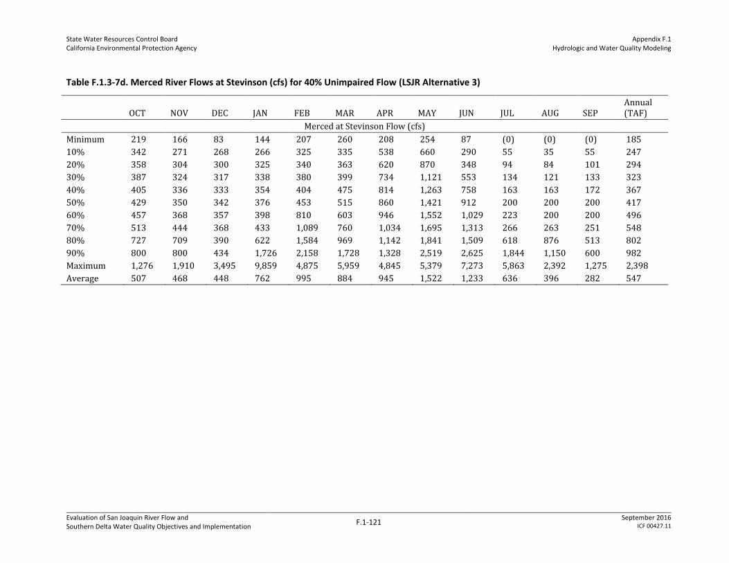
State Water Resources Control Board California Environmental Protection Agency
Appendix F.1 Hydrologic and Water Quality Modeling
Evaluation of San Joaquin River Flow and Southern Delta Water Quality Objectives and Implementation
F.1-121 September 2016
ICF 00427.11
Table F.1.3-7d. Merced River Flows at Stevinson (cfs) for 40% Unimpaired Flow (LSJR Alternative 3)
OCT NOV DEC JAN FEB MAR APR MAY JUN JUL AUG SEP Annual (TAF)
Merced at Stevinson Flow (cfs)
Minimum 219 166 83 144 207 260 208 254 87 (0) (0) (0) 185
10% 342 271 268 266 325 335 538 660 290 55 35 55 247
20% 358 304 300 325 340 363 620 870 348 94 84 101 294
30% 387 324 317 338 380 399 734 1,121 553 134 121 133 323
40% 405 336 333 354 404 475 814 1,263 758 163 163 172 367
50% 429 350 342 376 453 515 860 1,421 912 200 200 200 417
60% 457 368 357 398 810 603 946 1,552 1,029 223 200 200 496
70% 513 444 368 433 1,089 760 1,034 1,695 1,313 266 263 251 548
80% 727 709 390 622 1,584 969 1,142 1,841 1,509 618 876 513 802
90% 800 800 434 1,726 2,158 1,728 1,328 2,519 2,625 1,844 1,150 600 982
Maximum 1,276 1,910 3,495 9,859 4,875 5,959 4,845 5,379 7,273 5,863 2,392 1,275 2,398
Average 507 468 448 762 995 884 945 1,522 1,233 636 396 282 547
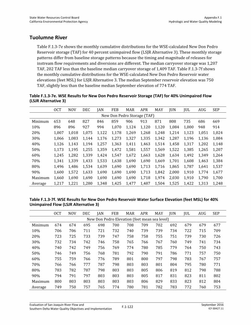
State Water Resources Control Board California Environmental Protection Agency
Appendix F.1 Hydrologic and Water Quality Modeling
Evaluation of San Joaquin River Flow and Southern Delta Water Quality Objectives and Implementation
F.1-122 September 2016
ICF 00427.11
Tuolumne River
Table F.1.3-7e shows the monthly cumulative distributions for the WSE-calculated New Don Pedro
Reservoir storage (TAF) for 40 percent unimpaired flow (LSJR Alternative 3). These monthly storage
patterns differ from baseline storage patterns because the timing and magnitude of releases for
instream flow requirements and diversions are different. The median carryover storage was 1,207
TAF, 202 TAF less than the baseline median carryover storage of 1,409 TAF. Table F.1.3-7f shows
the monthly cumulative distributions for the WSE-calculated New Don Pedro Reservoir water
elevations (feet MSL) for LSJR Alternative 3. The median September reservoir elevation was 750
TAF, slightly less than the baseline median September elevation of 774 TAF.
Table F.1.3-7e. WSE Results for New Don Pedro Reservoir Storage (TAF) for 40% Unimpaired Flow (LSJR Alternative 3)
OCT NOV DEC JAN FEB MAR APR MAY JUN JUL AUG SEP
New Don Pedro Storage (TAF)
Minimum 653 648 827 846 859 906 913 871 808 735 686 669
10% 896 896 927 994 1,070 1,124 1,120 1,120 1,084 1,000 948 914
20% 1,007 1,018 1,075 1,122 1,178 1,269 1,268 1,248 1,214 1,123 1,051 1,024
30% 1,066 1,083 1,144 1,176 1,273 1,327 1,335 1,342 1,287 1,196 1,136 1,084
40% 1,126 1,143 1,194 1,257 1,363 1,411 1,463 1,514 1,458 1,317 1,202 1,148
50% 1,173 1,195 1,255 1,359 1,472 1,581 1,557 1,569 1,522 1,385 1,265 1,207
60% 1,245 1,282 1,339 1,424 1,547 1,672 1,663 1,628 1,634 1,492 1,349 1,264
70% 1,341 1,339 1,433 1,533 1,638 1,690 1,690 1,669 1,701 1,608 1,463 1,384
80% 1,496 1,486 1,534 1,639 1,690 1,690 1,713 1,716 1,865 1,787 1,641 1,537
90% 1,600 1,572 1,633 1,690 1,690 1,690 1,713 1,842 2,000 1,910 1,774 1,677
Maximum 1,660 1,690 1,690 1,690 1,690 1,690 1,718 1,974 2,030 1,910 1,790 1,700
Average 1,217 1,221 1,280 1,348 1,425 1,477 1,487 1,504 1,525 1,422 1,313 1,248
Table F.1.3-7f. WSE Results for New Don Pedro Reservoir Water Surface Elevation (feet MSL) for 40% Unimpaired Flow (LSJR Alternative 3)
OCT NOV DEC JAN FEB MAR APR MAY JUN JUL AUG SEP
New Don Pedro Elevation (feet mean sea level)
Minimum 674 674 695 698 700 708 709 702 692 679 679 677
10% 706 706 711 721 732 740 739 739 734 722 715 709
20% 723 725 733 739 747 758 758 755 751 739 730 726
30% 732 734 742 746 758 765 766 767 760 749 741 734
40% 740 742 749 756 769 774 780 785 779 764 750 743
50% 746 749 756 768 781 792 790 791 786 771 757 750
60% 755 759 766 776 789 801 800 797 798 783 767 757
70% 766 766 777 787 798 803 803 801 804 795 780 771
80% 783 782 787 798 803 803 805 806 819 812 798 788
90% 794 791 797 803 803 803 805 817 831 823 811 802
Maximum 800 803 803 803 803 803 806 829 833 823 812 804
Average 749 750 757 765 774 780 781 782 783 772 760 753

State Water Resources Control Board California Environmental Protection Agency
Appendix F.1 Hydrologic and Water Quality Modeling
Evaluation of San Joaquin River Flow and Southern Delta Water Quality Objectives and Implementation
F.1-123 September 2016
ICF 00427.11
Table F.1.3-7g shows the monthly cumulative distributions for the WSE-calculated Tuolumne River
target flows at Modesto for LSJR Alternative 3. Target flows are the flows specified for the
downstream ends of the river in the absence of flood control releases. Comparison to the baseline
indicates that the average monthly target flows for LSJR Alternative 3 increased slightly from July–
November (as a result of adaptive implementation flow shifting) and remained unchanged during
December and January. From February through June, the average monthly target flows were higher
under the alternative compared to baseline because of the unimpaired flow requirement,
particularly in May and June. The greatest increase came in June when the average target flow
increased from 504 cfs under baseline to 2,231 cfs under the alternative.
Table F.1.3-7g. Tuolumne River Target Flows (cfs) for 40% Unimpaired Flow (LSJR Alternative 3)
OCT NOV DEC JAN FEB MAR APR MAY JUN JUL AUG SEP
Tuolumne Target Flow (cfs)
Minimum 199 206 71 208 235 338 531 690 283 194 187 166
10% 290 246 251 316 442 608 1,112 1,388 602 262 277 256
20% 395 324 319 417 505 738 1,293 1,894 913 319 346 334
30% 463 389 399 434 604 833 1,481 2,248 1,485 364 369 366
40% 499 452 430 479 647 925 1,632 2,439 1,846 403 403 381
50% 552 472 445 524 814 1,008 1,709 2,823 2,160 483 428 425
60% 681 562 496 572 940 1,116 1,804 3,013 2,583 582 586 574
70% 742 926 581 602 1,118 1,275 2,016 3,302 2,901 698 600 697
80% 1,000 1,000 602 648 1,662 1,545 2,183 3,497 3,232 1,200 600 1,000
90% 1,000 1,000 655 757 2,101 2,008 2,548 4,048 3,670 1,200 638 1,000
Maximum 1,171 1,530 1,405 2,411 4,164 3,484 4,063 5,693 6,531 1,200 760 1,000
Average 633 609 479 560 1,041 1,179 1,769 2,757 2,231 637 471 573
Table F.1.3-7h shows the monthly cumulative distributions for the WSE-calculated Tuolumne River
flows at Modesto for LSJR Alternative 3. The cumulative distributions of monthly flows were higher
than the target flows, indicating that flood control releases were sometimes required. However, only
about 44 percent of the years simulated required flood control releases, much less than under
baseline conditions, during which flood control releases occurred in about 66 percent of the years.

State Water Resources Control Board California Environmental Protection Agency
Appendix F.1 Hydrologic and Water Quality Modeling
Evaluation of San Joaquin River Flow and Southern Delta Water Quality Objectives and Implementation
F.1-124 September 2016
ICF 00427.11
Table F.1.3-7h. Tuolumne River Flows at Modesto (cfs) for 40% Unimpaired Flow (LSJR Alternative 3)
OCT NOV DEC JAN FEB MAR APR MAY JUN JUL AUG SEP Annual (TAF)
Tuolumne at Modesto Flow(cfs)
Minimum 199 206 217 208 235 338 531 690 283 194 187 166 261
10% 290 246 257 316 442 608 1,112 1,388 602 262 277 256 459
20% 395 324 322 427 511 801 1,293 1,894 913 319 346 334 560
30% 463 389 402 443 609 895 1,492 2,248 1,485 364 369 366 617
40% 499 452 431 518 722 1,014 1,659 2,439 1,846 403 403 381 678
50% 552 472 450 542 902 1,174 1,998 2,867 2,173 483 428 425 816
60% 681 562 518 593 1,188 1,661 2,236 3,117 2,583 582 586 574 918
70% 742 926 589 639 1,691 2,665 2,601 3,387 2,901 698 600 697 1,209
80% 1,000 1,000 611 836 2,583 3,463 3,183 3,538 3,334 1,200 600 1,000 1,425
90% 1,000 1,000 679 2,404 4,065 5,027 4,591 4,810 4,422 3,135 652 1,000 1,720
Maximum 3,090 5,440 7,479 17,925 6,927 16,297 9,332 9,474 7,110 8,047 2,996 2,296 4,129
Average 661 677 679 1,148 1,660 2,217 2,378 3,013 2,370 1,046 515 601 1,022

State Water Resources Control Board California Environmental Protection Agency
Appendix F.1 Hydrologic and Water Quality Modeling
Evaluation of San Joaquin River Flow and Southern Delta Water Quality Objectives and Implementation
F.1-125 September 2016
ICF 00427.11
Stanislaus River
Table F.1.3-7i shows the monthly cumulative distributions for the WSE-calculated New Melones
Reservoir storage (TAF) for LSJR Alternative 3. These monthly storage patterns differ from baseline
storage patterns because the timing and magnitude of releases for instream flow requirements and
diversions are different. The median carryover storage was 1,096 TAF, about 28 TAF less than the
baseline median carryover storage of 1,124 TAF. Table F.1.3-7j shows the monthly cumulative
distributions for the WSE-calculated New Melones Reservoir water surface elevations (feet MSL) for
LSJR Alternative 3. The median September reservoir elevation was 957 TAF under the alternative,
about the same as the baseline median September elevation of 961 TAF.
Table F.1.3-7i. WSE Results for New Melones Reservoir Storage (TAF) for 40% Unimpaired Flow (LSJR Alternative 3)
OCT NOV DEC JAN FEB MAR APR MAY JUN JUL AUG SEP
New Melones Reservoir Storage (TAF)
Minimum 636 648 661 737 748 784 767 704 691 679 662 662
10% 754 766 788 809 852 902 877 864 849 825 795 781
20% 824 830 858 872 906 968 949 929 964 949 891 854
30% 884 901 932 1,009 1,031 1,058 1,077 1,069 1,062 1,011 948 924
40% 988 1,001 1,045 1,094 1,128 1,208 1,214 1,211 1,178 1,123 1,067 1,028
50% 1,042 1,081 1,127 1,202 1,296 1,363 1,402 1,357 1,323 1,215 1,132 1,096
60% 1,141 1,178 1,235 1,361 1,418 1,476 1,477 1,493 1,447 1,332 1,235 1,193
70% 1,344 1,364 1,394 1,450 1,533 1,552 1,553 1,594 1,648 1,568 1,479 1,415
80% 1,489 1,494 1,546 1,607 1,649 1,734 1,717 1,705 1,753 1,690 1,596 1,539
90% 1,658 1,668 1,695 1,725 1,811 1,901 1,936 1,949 1,924 1,827 1,749 1,710
Maximum 1,970 1,970 1,970 1,970 1,970 2,030 2,090 2,137 2,385 2,300 2,130 2,000
Average 1,145 1,160 1,198 1,254 1,308 1,354 1,352 1,360 1,363 1,297 1,227 1,188
Table F.1.3-7j. WSE Results for New Melones Reservoir Water Surface Elevation (feet MSL) for 40% Unimpaired Flow (LSJR Alternative 3)
OCT NOV DEC JAN FEB MAR APR MAY JUN JUL AUG SEP
New Melones Elevation (feet mean sea level)
Minimum 875 878 881 896 899 906 902 890 887 884 881 881
10% 900 902 906 910 918 926 922 920 917 913 908 905
20% 913 914 919 922 927 937 934 931 937 934 925 918
30% 924 926 932 944 947 951 954 953 952 944 934 930
40% 940 942 949 956 961 972 973 972 968 960 952 947
50% 949 954 961 971 983 991 996 991 986 973 962 957
60% 963 968 975 991 998 1,004 1,004 1,006 1,001 987 975 970
70% 989 991 995 1,001 1,010 1,012 1,013 1,017 1,022 1,014 1,005 997
80% 1,006 1,006 1,012 1,018 1,022 1,031 1,029 1,028 1,033 1,027 1,017 1,011
90% 1,023 1,024 1,027 1,030 1,038 1,047 1,050 1,051 1,049 1,040 1,032 1,029
Maximum 1,053 1,053 1,053 1,053 1,053 1,058 1,063 1,067 1,086 1,080 1,066 1,055
Average 957 960 965 972 979 985 984 985 985 977 968 963

State Water Resources Control Board California Environmental Protection Agency
Appendix F.1 Hydrologic and Water Quality Modeling
Evaluation of San Joaquin River Flow and Southern Delta Water Quality Objectives and Implementation
F.1-126 September 2016
ICF 00427.11
Table F.1.3-7k shows the monthly cumulative distributions for the WSE-calculated Stanislaus River
target flows at Ripon for LSJR Alternative 3. Target flows are the flows specified for the downstream
ends of the river in the absence of flood control releases. Comparison to the baseline indicates that
the average monthly target flows under LSJR Alternative 3 remained mostly unchanged from July to
February (except in October), with some differences because of changes in the NMI under the
alternative. October targets were higher as a result of adaptive implementation flow shifting in
order to control potential temperature effects during summer and fall. From February to June, the
average monthly target flows were generally higher than under baseline. The greatest increase came
in May when the average target flow increased from 1,328 cfs under baseline to 1,771 cfs under the
alternative.
Table F.1.3-7k. Stanislaus River Target Flows (cfs) for 40% Unimpaired Flow (LSJR Alternative 3)
OCT NOV DEC JAN FEB MAR APR MAY JUN JUL AUG SEP
Stanislaus Target Flow (cfs)
Minimum 763 213 94 129 225 238 460 443 205 205 208 174
10% 800 248 225 267 268 371 693 756 315 307 312 299
20% 1,000 260 243 294 340 462 955 1,084 442 325 352 358
30% 1,000 267 263 310 389 516 1,230 1,346 608 357 370 377
40% 1,000 292 280 323 445 599 1,395 1,610 864 395 410 397
50% 1,122 318 288 335 519 692 1,539 1,782 1,114 437 425 421
60% 1,200 336 305 347 705 813 1,687 2,003 1,261 534 471 476
70% 1,204 348 320 360 778 1,162 1,744 2,109 1,365 682 500 700
80% 1,400 379 368 397 921 1,711 1,822 2,265 1,590 800 512 800
90% 1,400 445 423 502 1,409 1,897 1,928 2,711 2,050 800 554 800
Maximum 1,409 732 1,071 884 3,832 2,636 2,766 3,752 4,189 1,021 732 887
Average 1,121 326 323 358 730 967 1,440 1,771 1,139 524 439 515
Table F.1.3-7l shows the monthly cumulative distributions for the WSE-calculated Stanislaus River
flows at Ripon for LSJR Alternative 3. The monthly flows were higher than the target flows for some
of the higher cumulative distribution values, indicating that flood control releases were sometimes
required. However, only about 7 percent of the years required some flood control releases.

State Water Resources Control Board California Environmental Protection Agency
Appendix F.1 Hydrologic and Water Quality Modeling
Evaluation of San Joaquin River Flow and Southern Delta Water Quality Objectives and Implementation
F.1-127 September 2016
ICF 00427.11
Table F.1.3-7l. Stanislaus River Flows at Ripon (cfs) for 40% Unimpaired Flow (LSJR Alternative 3)
OCT NOV DEC JAN FEB MAR APR MAY JUN JUL AUG SEP Annual (TAF)
Stanislaus at Ripon Flow (cfs)
Minimum 763 213 94 129 225 238 460 443 205 205 208 174 253
10% 800 248 225 267 268 371 693 756 315 307 312 299 325
20% 1,000 260 247 295 340 462 955 1,084 442 325 352 358 406
30% 1,000 267 267 312 389 516 1,230 1,346 608 357 370 377 457
40% 1,000 292 280 324 445 599 1,395 1,610 864 395 410 397 519
50% 1,122 318 291 336 519 692 1,539 1,782 1,114 437 425 421 591
60% 1,200 336 306 349 730 813 1,687 2,003 1,261 534 471 476 619
70% 1,204 348 320 362 788 1,162 1,744 2,109 1,365 682 500 700 686
80% 1,400 379 368 414 1,196 1,711 1,822 2,265 1,590 800 512 800 760
90% 1,400 445 423 541 1,799 1,897 1,928 2,711 2,050 800 554 800 930
Maximum 1,538 3,453 5,126 10,555 5,177 6,223 2,766 3,752 4,189 3,770 2,664 3,050 2,453
Average 1,123 382 417 582 878 1,011 1,440 1,771 1,139 560 462 551 622

State Water Resources Control Board California Environmental Protection Agency
Appendix F.1 Hydrologic and Water Quality Modeling
Evaluation of San Joaquin River Flow and Southern Delta Water Quality Objectives and Implementation
F.1-128 September 2016
ICF 00427.11
SJR at Vernalis
Table F.1.3-7m shows the monthly cumulative distributions for the WSE-calculated SJR at Vernalis
flows for LSJR Alternative 3. The average Vernalis flows were similar to the baseline flows in
February and March but were 810–2,400 cfs higher from April–June. LSJR Alternative 3 provided a
more natural distribution of flows from February–June, and the average annual flow volume was
294 TAF more than the average baseline flow volume at Vernalis (10 percent higher).

State Water Resources Control Board California Environmental Protection Agency
Appendix F.1 Hydrologic and Water Quality Modeling
Evaluation of San Joaquin River Flow and Southern Delta Water Quality Objectives and Implementation
F.1-129 September 2016
ICF 00427.11
Table F.1.3-7m. SJR Flows at Vernalis (cfs) for 40% Unimpaired Flow (LSJR Alternative 3)
OCT NOV DEC JAN FEB MAR APR MAY JUN JUL AUG SEP Annual (TAF)
SJR at Vernalis Flow (cfs)
Minimum 1,539 1,233 1,238 1,146 1,526 1,124 1,349 1,724 1,000 525 579 955 956
10% 2,000 1,566 1,513 1,480 1,852 1,742 2,788 3,220 1,537 955 1,054 1,459 1,465
20% 2,263 1,696 1,657 1,699 2,033 2,453 3,747 4,456 2,199 1,139 1,248 1,685 1,773
30% 2,451 1,795 1,789 1,886 2,316 2,775 4,219 5,349 3,083 1,226 1,341 1,796 1,924
40% 2,571 1,906 1,884 2,113 2,636 3,310 4,796 6,154 4,169 1,439 1,449 1,913 2,098
50% 2,832 1,998 1,941 2,167 3,073 3,949 5,394 7,330 5,061 1,633 1,568 2,030 2,504
60% 3,066 2,170 2,035 2,352 5,426 5,367 5,986 8,009 5,604 1,865 1,767 2,180 2,922
70% 3,473 2,706 2,157 3,024 6,679 6,733 6,926 9,125 6,197 2,289 2,081 2,971 3,412
80% 3,876 3,121 2,555 4,020 8,828 8,674 8,553 9,992 7,796 3,305 2,539 3,331 4,524
90% 3,987 3,344 3,029 9,349 12,232 13,701 13,460 15,878 11,927 6,345 2,984 3,543 5,492
Maximum 6,343 16,297 24,021 62,587 34,271 48,485 27,192 27,339 29,234 20,781 9,143 7,677 15,840
Average 2,990 2,528 2,869 4,425 6,194 6,596 6,795 8,378 6,011 3,036 1,904 2,401 3,259

State Water Resources Control Board California Environmental Protection Agency
Appendix F.1 Hydrologic and Water Quality Modeling
Evaluation of San Joaquin River Flow and Southern Delta Water Quality Objectives and Implementation
F.1-130 September 2016
ICF 00427.11
F.1.3.5 60 Percent Unimpaired Flow (LSJR Alternative 4)
The WSE model was used to simulate 60 percent unimpaired flow, which represents typical
conditions for LSJR Alternative 4. For this simulation, LSJR tributary flows were greater than or
equal to 60 percent of the unimpaired reservoir inflow from February–June. Some of the February–
June flow was reserved for controlling potential temperature effects later in the year; thus, resulting
flows may decrease slightly below 60 percent of unimpaired flow during some years. In some years,
February–June flows were higher than the 60 percent unimpaired flow objective because of flood
control releases or other flow requirements. The reservoir storage and water supply diversions
were adjusted to satisfy these monthly flow objectives for each of the eastside tributaries. Flood
control releases in many years were reduced or eliminated because higher flows were released from
February–June to satisfy the flow objectives. Water supply diversions were reduced in many years
to account for the 60 percent unimpaired flow requirement and maintain storage in the reservoirs.
Merced River
Table F.1.3-8a shows the monthly cumulative distributions for the WSE-calculated Lake McClure
storage (TAF) for LSJR Alternative 4. These monthly storage patterns differ from baseline storage
patterns because the timing and magnitude of releases for instream flow requirements and
diversions are different. The median carryover storage was 475 TAF, about 24 TAF more than the
baseline median carryover storage of 451 TAF. Table F.1.3-8b shows the monthly cumulative
distributions for the WSE-calculated Lake McClure water surface elevations (feet MSL) for LSJR
Alternative 4. The median September reservoir elevation was 764 TAF, slightly higher than the
baseline median September elevation of 757 TAF.
Table F.1.3-8a. WSE Results for Lake McClure Storage (TAF) for 60% Unimpaired Flow (LSJR Alternative 4)
OCT NOV DEC JAN FEB MAR APR MAY JUN JUL AUG SEP
Lake McClure Storage (TAF)
Minimum 52 35 52 102 99 132 141 167 147 128 101 80
10% 269 264 264 264 288 318 339 291 303 321 305 292
20% 299 295 292 319 350 364 375 407 405 377 350 325
30% 376 374 389 394 402 394 420 461 482 456 410 397
40% 416 411 426 444 467 476 495 554 537 493 450 422
50% 446 442 460 483 534 550 571 611 615 575 515 475
60% 472 465 485 522 600 630 655 671 689 630 546 503
70% 501 495 522 587 637 681 698 737 728 677 588 541
80% 529 528 574 645 675 720 759 811 828 740 627 568
90% 631 597 637 675 675 735 797 875 964 910 770 689
Maximum 675 675 675 675 675 735 845 970 1,024 910 770 700
Average 431 424 444 473 503 530 559 602 612 568 502 462

State Water Resources Control Board California Environmental Protection Agency
Appendix F.1 Hydrologic and Water Quality Modeling
Evaluation of San Joaquin River Flow and Southern Delta Water Quality Objectives and Implementation
F.1-131 September 2016
ICF 00427.11
Table F.1.3-8b. WSE Results for Lake McClure Water Surface Elevations (feet MSL) for 60% Unimpaired Flow (LSJR Alternative 4)
OCT NOV DEC JAN FEB MAR APR MAY JUN JUL AUG SEP
Lake McClure Elevation (feet mean sea level)
Minimum 567 538 567 619 617 640 646 660 649 638 618 599
10% 695 693 693 693 703 715 722 704 709 716 710 705
20% 708 706 705 715 726 731 735 745 744 735 726 717
30% 735 734 739 741 743 741 748 760 766 759 745 742
40% 747 746 750 755 762 764 769 783 779 768 757 749
50% 756 755 760 766 779 783 787 796 797 788 774 764
60% 763 761 766 776 794 800 805 809 812 800 782 771
70% 771 769 776 791 802 811 814 821 820 810 791 780
80% 777 777 788 803 809 818 825 834 837 822 800 787
90% 800 793 802 809 809 821 832 845 858 850 827 812
Maximum 809 809 809 809 809 821 840 859 867 850 827 814
Average 746 743 749 757 765 772 778 787 788 779 765 755
Table F.1.3-8c shows the monthly cumulative distributions for the WSE-calculated Merced River
target flows at Stevinson for LSJR Alternative 4. Target flows are the flows specified for the
downstream ends of the river in the absence of flood control releases. Comparison to the baseline
indicates that the average monthly target flows for LSJR Alternative 4 increased from July–
November (as a result of adaptive implementation flow shifting) and remained unchanged during
December and January. From February through June, the average monthly target flows were higher
in the alternative compared to baseline because of the unimpaired flow requirement, particularly
from April–June. The greatest increase came in May when the average target flow increased from
341 cfs under baseline to 2,164 cfs under the alternative.
Table F.1.3-8c. Merced River Target Flows (cfs) for 60% Unimpaired Flow (LSJR Alternative 4)
OCT NOV DEC JAN FEB MAR APR MAY JUN JUL AUG SEP
Merced Target Flow (cfs)
Minimum 219 166 33 99 207 281 313 381 131 (0) (0) (0)
10% 342 271 263 260 332 391 807 989 435 55 35 55
20% 358 304 287 318 360 505 930 1,306 522 94 84 101
30% 387 324 309 332 397 576 1,101 1,681 829 134 121 133
40% 405 336 332 345 488 637 1,245 1,918 1,137 163 163 172
50% 429 350 338 360 557 769 1,308 2,192 1,377 200 200 200
60% 457 368 352 386 706 877 1,462 2,431 1,574 223 200 200
70% 569 444 363 424 903 1,002 1,589 2,604 2,016 266 263 251
80% 800 800 381 482 1,379 1,235 1,735 2,808 2,386 600 600 600
90% 800 800 409 560 1,961 1,442 1,961 3,191 2,703 600 600 600
Maximum 1,276 847 1,075 1,730 3,406 3,567 4,055 4,719 6,535 1,133 600 629
Average 517 461 344 416 873 911 1,379 2,164 1,563 281 267 274
State Water Resources Control Board California Environmental Protection Agency
Appendix F.1 Hydrologic and Water Quality Modeling
Evaluation of San Joaquin River Flow and Southern Delta Water Quality Objectives and Implementation
F.1-132 September 2016
ICF 00427.11
Table F.1.3-8d shows the monthly cumulative distributions for the WSE-calculated Merced River
flows at Stevinson for LSJR Alternative 4. The monthly flows were greater than the target flows for
some of the higher cumulative distribution values, but this occurred less often than under baseline
conditions. This indicates that flood control releases were required in fewer years than under
baseline. Under LSJR Alternative 4, about 28 percent of years required flood control releases
compared to about 50 percent of years under baseline.

State Water Resources Control Board California Environmental Protection Agency
Appendix F.1 Hydrologic and Water Quality Modeling
Evaluation of San Joaquin River Flow and Southern Delta Water Quality Objectives and Implementation
F.1-133 September 2016
ICF 00427.11
Table F.1.3-8d. Merced River Flows at Stevinson (cfs) for 60% Unimpaired Flow (LSJR Alternative 4)
OCT NOV DEC JAN FEB MAR APR MAY JUN JUL AUG SEP Annual (TAF)
Merced at Stevinson Flow (cfs)
Minimum 219 166 196 144 207 281 313 381 131 (0) (0) (0) 209
10% 342 271 273 261 332 391 807 989 435 55 35 55 316
20% 358 304 301 323 360 505 930 1,306 522 94 84 101 379
30% 387 324 317 334 410 576 1,101 1,681 829 134 121 133 401
40% 405 336 333 352 497 637 1,245 1,918 1,137 163 163 172 474
50% 429 350 342 370 581 769 1,308 2,192 1,377 200 200 200 560
60% 457 368 357 395 881 913 1,462 2,431 1,574 223 200 200 640
70% 569 444 368 432 1,411 1,010 1,589 2,604 2,016 266 263 251 708
80% 800 800 389 521 1,844 1,350 1,735 2,808 2,386 600 600 600 860
90% 800 800 427 1,522 2,368 1,731 1,961 3,191 2,703 908 1,073 600 1,015
Maximum 1,276 1,910 3,495 9,859 4,474 5,959 4,845 5,120 6,535 5,048 2,392 1,073 2,398
Average 521 484 424 728 1,097 1,045 1,388 2,169 1,571 508 362 287 637

State Water Resources Control Board California Environmental Protection Agency
Appendix F.1 Hydrologic and Water Quality Modeling
Evaluation of San Joaquin River Flow and Southern Delta Water Quality Objectives and Implementation
F.1-134 September 2016
ICF 00427.11
Tuolumne River
Table F.1.3-8e shows the monthly cumulative distributions for the WSE-calculated New Don Pedro
Reservoir storage (TAF) for LSJR Alternative 4. These monthly storage patterns differ from baseline
storage patterns because the timing and magnitude of releases for instream flow requirements and
diversions are different. The median carryover storage was 1,192 TAF, lower than the baseline
median carryover storage of 1,409 TAF. Table F.1.3-8f shows the monthly cumulative distributions
for the WSE-calculated New Don Pedro Reservoir water surface elevations (feet MSL) for LSJR
Alternative 4. The median September reservoir elevation was 748 TAF, slightly less than the
baseline median September elevation of 774 TAF.
Table F.1.3-8e. WSE Results for New Don Pedro Reservoir Storage (TAF) for 60% Unimpaired Flow (LSJR Alternative 4)
OCT NOV DEC JAN FEB MAR APR MAY JUN JUL AUG SEP
New Don Pedro Reservoir Storage (TAF)
Minimum 735 733 793 937 935 951 945 893 815 774 750 745
10% 962 964 997 1,027 1,087 1,130 1,110 1,082 1,043 1,009 986 979
20% 1,026 1,048 1,069 1,117 1,189 1,247 1,226 1,169 1,146 1,091 1,048 1,027
30% 1,081 1,076 1,144 1,198 1,256 1,304 1,287 1,277 1,233 1,185 1,124 1,098
40% 1,137 1,143 1,183 1,256 1,309 1,355 1,365 1,326 1,302 1,253 1,185 1,157
50% 1,175 1,176 1,247 1,297 1,379 1,453 1,410 1,435 1,434 1,344 1,247 1,192
60% 1,221 1,242 1,300 1,353 1,451 1,555 1,598 1,510 1,493 1,409 1,314 1,249
70% 1,282 1,297 1,366 1,457 1,571 1,638 1,646 1,556 1,532 1,444 1,343 1,297
80% 1,316 1,360 1,461 1,593 1,688 1,690 1,690 1,640 1,631 1,618 1,472 1,356
90% 1,524 1,482 1,565 1,690 1,690 1,690 1,705 1,729 1,792 1,814 1,683 1,590
Maximum 1,660 1,690 1,690 1,690 1,690 1,690 1,713 1,874 1,943 1,910 1,790 1,700
Average 1,196 1,202 1,263 1,333 1,395 1,439 1,440 1,408 1,402 1,352 1,271 1,223
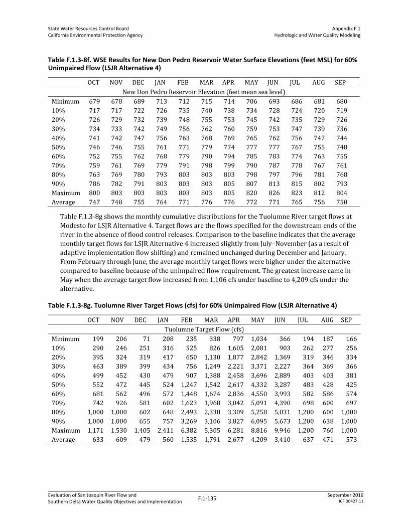
State Water Resources Control Board California Environmental Protection Agency
Appendix F.1 Hydrologic and Water Quality Modeling
Evaluation of San Joaquin River Flow and Southern Delta Water Quality Objectives and Implementation
F.1-135 September 2016
ICF 00427.11
Table F.1.3-8f. WSE Results for New Don Pedro Reservoir Water Surface Elevations (feet MSL) for 60% Unimpaired Flow (LSJR Alternative 4)
OCT NOV DEC JAN FEB MAR APR MAY JUN JUL AUG SEP
New Don Pedro Reservoir Elevation (feet mean sea level)
Minimum 679 678 689 713 712 715 714 706 693 686 681 680
10% 717 717 722 726 735 740 738 734 728 724 720 719
20% 726 729 732 739 748 755 753 745 742 735 729 726
30% 734 733 742 749 756 762 760 759 753 747 739 736
40% 741 742 747 756 763 768 769 765 762 756 747 744
50% 746 746 755 761 771 779 774 777 777 767 755 748
60% 752 755 762 768 779 790 794 785 783 774 763 755
70% 759 761 769 779 791 798 799 790 787 778 767 761
80% 763 769 780 793 803 803 803 798 797 796 781 768
90% 786 782 791 803 803 803 805 807 813 815 802 793
Maximum 800 803 803 803 803 803 805 820 826 823 812 804
Average 747 748 755 764 771 776 776 772 771 765 756 750
Table F.1.3-8g shows the monthly cumulative distributions for the Tuolumne River target flows at
Modesto for LSJR Alternative 4. Target flows are the flows specified for the downstream ends of the
river in the absence of flood control releases. Comparison to the baseline indicates that the average
monthly target flows for LSJR Alternative 4 increased slightly from July–November (as a result of
adaptive implementation flow shifting) and remained unchanged during December and January.
From February through June, the average monthly target flows were higher under the alternative
compared to baseline because of the unimpaired flow requirement. The greatest increase came in
May when the average target flow increased from 1,106 cfs under baseline to 4,209 cfs under the
alternative.
Table F.1.3-8g. Tuolumne River Target Flows (cfs) for 60% Unimpaired Flow (LSJR Alternative 4)
OCT NOV DEC JAN FEB MAR APR MAY JUN JUL AUG SEP
Tuolumne Target Flow (cfs)
Minimum 199 206 71 208 235 338 797 1,034 366 194 187 166
10% 290 246 251 316 525 826 1,605 2,081 903 262 277 256
20% 395 324 319 417 650 1,130 1,877 2,842 1,369 319 346 334
30% 463 389 399 434 756 1,249 2,221 3,371 2,227 364 369 366
40% 499 452 430 479 907 1,388 2,458 3,696 2,889 403 403 381
50% 552 472 445 524 1,247 1,542 2,617 4,332 3,287 483 428 425
60% 681 562 496 572 1,448 1,674 2,836 4,550 3,993 582 586 574
70% 742 926 581 602 1,623 1,968 3,042 5,091 4,390 698 600 697
80% 1,000 1,000 602 648 2,493 2,338 3,309 5,258 5,031 1,200 600 1,000
90% 1,000 1,000 655 757 3,269 3,106 3,827 6,095 5,673 1,200 638 1,000
Maximum 1,171 1,530 1,405 2,411 6,382 5,305 6,281 8,816 9,946 1,200 760 1,000
Average 633 609 479 560 1,535 1,791 2,677 4,209 3,410 637 471 573

State Water Resources Control Board California Environmental Protection Agency
Appendix F.1 Hydrologic and Water Quality Modeling
Evaluation of San Joaquin River Flow and Southern Delta Water Quality Objectives and Implementation
F.1-136 September 2016
ICF 00427.11
Table F.1.3-8h shows the monthly cumulative distributions for the WSE-calculated Tuolumne River
flows at Modesto for LSJR Alternative 4. The cumulative distributions of monthly flows were higher
than the target flows in some months, indicating that flood control releases were sometimes
required. However, only about 29 percent of years had flood control releases under LSJR
Alternative 4 compared to 66 percent of years under baseline.

State Water Resources Control Board California Environmental Protection Agency
Appendix F.1 Hydrologic and Water Quality Modeling
Evaluation of San Joaquin River Flow and Southern Delta Water Quality Objectives and Implementation
F.1-137 September 2016
ICF 00427.11
Table F.1.3-8h. Tuolumne River Flows at Modesto (cfs) for 60% Unimpaired Flow (LSJR Alternative 4)
OCT NOV DEC JAN FEB MAR APR MAY JUN JUL AUG SEP Annual (TAF)
Tuolumne at Modesto Flow (cfs)
Minimum 199 206 217 208 235 338 797 1,034 366 194 187 166 319
10% 290 246 257 316 525 826 1,605 2,081 903 262 277 256 594
20% 395 324 322 427 650 1,130 1,877 2,842 1,369 319 346 334 739
30% 463 389 402 443 772 1,255 2,221 3,371 2,227 364 369 366 805
40% 499 452 431 518 971 1,413 2,458 3,696 2,889 403 403 381 913
50% 552 472 450 549 1,296 1,615 2,652 4,359 3,287 483 428 425 1,088
60% 681 562 518 595 1,712 1,928 2,937 4,684 3,993 582 586 574 1,256
70% 742 926 589 639 2,488 2,846 3,197 5,107 4,390 698 600 697 1,384
80% 1,000 1,000 611 748 3,291 3,544 3,545 5,338 5,031 1,200 600 1,000 1,588
90% 1,000 1,000 679 2,200 3,963 4,421 4,105 6,355 5,673 1,200 652 1,000 1,916
Maximum 3,090 5,440 7,479 17,925 6,917 16,297 9,332 8,816 9,946 5,424 2,123 2,296 4,131
Average 661 677 664 1,142 1,963 2,420 2,861 4,268 3,410 795 504 601 1,202

State Water Resources Control Board California Environmental Protection Agency
Appendix F.1 Hydrologic and Water Quality Modeling
Evaluation of San Joaquin River Flow and Southern Delta Water Quality Objectives and Implementation
F.1-138 September 2016
ICF 00427.11
Stanislaus River
Table F.1.3-8i shows the monthly cumulative distributions for the WSE-calculated New Melones
Reservoir storage (TAF) for LSJR Alternative 4. These monthly storage patterns differ from baseline
storage patterns because the timing and magnitude of releases for instream flow requirements and
diversions are different. The median carryover storage was 1,026 TAF, about 98 TAF lower than the
baseline median carryover storage of 1,124 TAF. Table F.1.3-8j shows the monthly cumulative
distributions for the WSE-calculated New Melones Reservoir water surface elevations (feet MSL) for
LSJR Alternative 4. The median September reservoir elevation was 946 TAF under the alternative,
slightly lower than the baseline median September elevation of 961 TAF.
Table F.1.3-8i. WSE Results for New Melones Reservoir Storage (TAF) for 60% Unimpaired Flow (LSJR Alternative 4)
OCT NOV DEC JAN FEB MAR APR MAY JUN JUL AUG SEP
New Melones Reservoir Storage (TAF)
Minimum 599 601 603 719 744 757 714 656 642 627 615 613
10% 782 783 803 850 888 909 862 843 833 808 795 802
20% 834 853 872 916 940 951 919 880 898 883 858 857
30% 900 912 937 960 988 999 1,001 972 999 966 946 936
40% 944 962 997 1,037 1,087 1,121 1,097 1,062 1,065 1,031 996 974
50% 968 994 1,036 1,101 1,145 1,190 1,185 1,158 1,139 1,078 1,039 1,026
60% 1,034 1,064 1,109 1,202 1,241 1,265 1,242 1,250 1,232 1,181 1,098 1,072
70% 1,117 1,157 1,211 1,277 1,330 1,357 1,358 1,351 1,350 1,254 1,202 1,182
80% 1,250 1,263 1,299 1,444 1,509 1,526 1,524 1,512 1,486 1,415 1,328 1,294
90% 1,449 1,469 1,518 1,591 1,646 1,720 1,764 1,776 1,749 1,630 1,545 1,503
Maximum 1,970 1,970 1,970 1,970 1,970 2,030 2,065 2,011 2,133 2,232 2,130 2,000
Average 1,048 1,067 1,110 1,174 1,216 1,250 1,233 1,208 1,201 1,161 1,113 1,087
Table F.1.3-8j. WSE Results for New Melones Reservoir Water Surface Elevations (feet MSL) for 60% Unimpaired Flow (LSJR Alternative 4)
OCT NOV DEC JAN FEB MAR APR MAY JUN JUL AUG SEP
New Melones Reservoir Elevation (feet mean sea level)
Minimum 867 867 867 893 898 900 892 880 877 873 870 870
10% 905 905 909 918 924 928 920 916 915 910 908 909
20% 915 918 921 929 933 935 929 923 926 923 919 919
30% 926 928 932 936 940 942 942 938 942 937 934 932
40% 933 936 942 948 955 960 957 952 952 947 942 938
50% 937 941 948 957 963 969 969 965 963 954 948 946
60% 947 952 958 971 976 979 976 977 975 968 957 953
70% 959 965 972 981 987 990 991 990 990 978 971 968
80% 977 979 983 1,001 1,008 1,010 1,009 1,008 1,005 997 987 983
90% 1,001 1,003 1,009 1,017 1,022 1,030 1,034 1,035 1,032 1,021 1,012 1,007
Maximum 1,053 1,053 1,053 1,053 1,053 1,058 1,061 1,056 1,066 1,074 1,066 1,055
Average 946 949 955 963 969 973 971 967 966 961 955 952
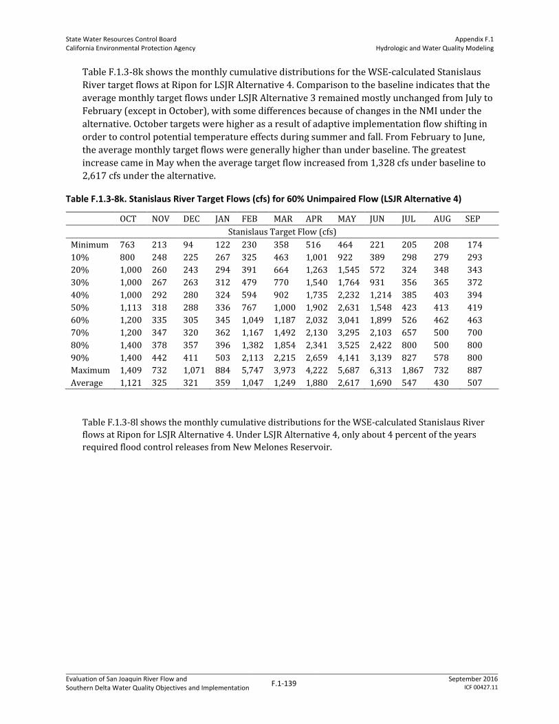
State Water Resources Control Board California Environmental Protection Agency
Appendix F.1 Hydrologic and Water Quality Modeling
Evaluation of San Joaquin River Flow and Southern Delta Water Quality Objectives and Implementation
F.1-139 September 2016
ICF 00427.11
Table F.1.3-8k shows the monthly cumulative distributions for the WSE-calculated Stanislaus
River target flows at Ripon for LSJR Alternative 4. Comparison to the baseline indicates that the
average monthly target flows under LSJR Alternative 3 remained mostly unchanged from July to
February (except in October), with some differences because of changes in the NMI under the
alternative. October targets were higher as a result of adaptive implementation flow shifting in
order to control potential temperature effects during summer and fall. From February to June,
the average monthly target flows were generally higher than under baseline. The greatest
increase came in May when the average target flow increased from 1,328 cfs under baseline to
2,617 cfs under the alternative.
Table F.1.3-8k. Stanislaus River Target Flows (cfs) for 60% Unimpaired Flow (LSJR Alternative 4)
OCT NOV DEC JAN FEB MAR APR MAY JUN JUL AUG SEP
Stanislaus Target Flow (cfs)
Minimum 763 213 94 122 230 358 516 464 221 205 208 174
10% 800 248 225 267 325 463 1,001 922 389 298 279 293
20% 1,000 260 243 294 391 664 1,263 1,545 572 324 348 343
30% 1,000 267 263 312 479 770 1,540 1,764 931 356 365 372
40% 1,000 292 280 324 594 902 1,735 2,232 1,214 385 403 394
50% 1,113 318 288 336 767 1,000 1,902 2,631 1,548 423 413 419
60% 1,200 335 305 345 1,049 1,187 2,032 3,041 1,899 526 462 463
70% 1,200 347 320 362 1,167 1,492 2,130 3,295 2,103 657 500 700
80% 1,400 378 357 396 1,382 1,854 2,341 3,525 2,422 800 500 800
90% 1,400 442 411 503 2,113 2,215 2,659 4,141 3,139 827 578 800
Maximum 1,409 732 1,071 884 5,747 3,973 4,222 5,687 6,313 1,867 732 887
Average 1,121 325 321 359 1,047 1,249 1,880 2,617 1,690 547 430 507
Table F.1.3-8l shows the monthly cumulative distributions for the WSE-calculated Stanislaus River
flows at Ripon for LSJR Alternative 4. Under LSJR Alternative 4, only about 4 percent of the years
required flood control releases from New Melones Reservoir.

State Water Resources Control Board California Environmental Protection Agency
Appendix F.1 Hydrologic and Water Quality Modeling
Evaluation of San Joaquin River Flow and Southern Delta Water Quality Objectives and Implementation
F.1-140 September 2016
ICF 00427.11
Table F.1.3-8l. Stanislaus River Flows at Ripon (cfs) for 60% Unimpaired Flow (LSJR Alternative 4)
OCT NOV DEC JAN FEB MAR APR MAY JUN JUL AUG SEP Annual (TAF)
Stanislaus at Ripon Flow (cfs)
Minimum 763 213 94 122 230 358 516 464 221 205 208 174 258
10% 800 248 225 267 325 463 1,001 922 389 298 279 293 392
20% 1,000 260 243 295 391 664 1,263 1,545 572 324 348 343 496
30% 1,000 267 263 314 479 770 1,540 1,764 931 356 365 372 540
40% 1,000 292 280 325 594 902 1,735 2,232 1,214 385 403 394 652
50% 1,113 318 288 339 767 1,000 1,902 2,631 1,548 423 413 419 725
60% 1,200 335 305 347 1,096 1,187 2,032 3,041 1,899 526 462 463 806
70% 1,200 347 320 364 1,182 1,492 2,130 3,295 2,103 657 500 700 896
80% 1,400 378 357 405 1,731 1,854 2,341 3,525 2,422 800 500 800 947
90% 1,400 442 411 526 2,250 2,215 2,659 4,141 3,139 827 578 800 1,166
Maximum 1,538 3,453 5,126 6,009 5,747 6,223 4,222 5,687 6,313 1,867 1,560 3,050 2,162
Average 1,122 361 377 482 1,127 1,277 1,880 2,617 1,690 547 440 534 750

State Water Resources Control Board California Environmental Protection Agency
Appendix F.1 Hydrologic and Water Quality Modeling
Evaluation of San Joaquin River Flow and Southern Delta Water Quality Objectives and Implementation
F.1-141 September 2016
ICF 00427.11
SJR at Vernalis
Table F.1.3-8m shows the monthly cumulative distributions for the WSE-calculated SJR at Vernalis
flows for LSJR Alternative 4. The average Vernalis flows for LSJR Alternative 4 were much higher
than the baseline flows from February–June. LSJR Alternative 4 provided a more natural distribution
of flows from February–June. The average annual flow volume was 693 TAF more than the average
annual baseline flow volume at Vernalis (19 percent higher).
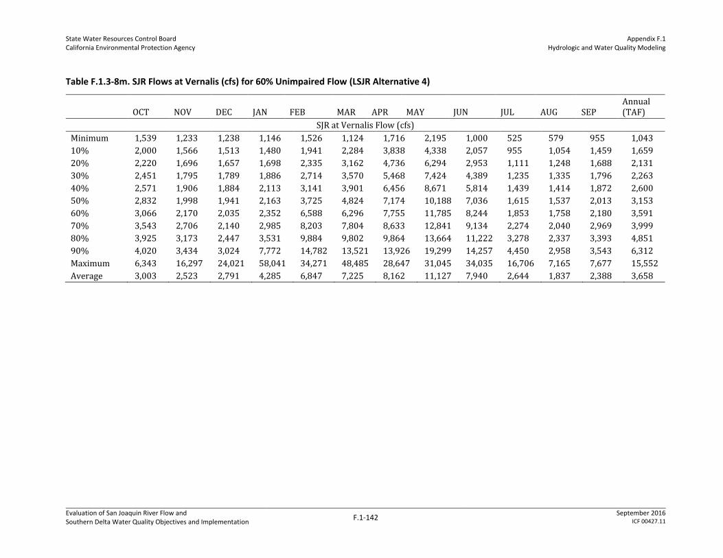
State Water Resources Control Board California Environmental Protection Agency
Appendix F.1 Hydrologic and Water Quality Modeling
Evaluation of San Joaquin River Flow and Southern Delta Water Quality Objectives and Implementation
F.1-142 September 2016
ICF 00427.11
Table F.1.3-8m. SJR Flows at Vernalis (cfs) for 60% Unimpaired Flow (LSJR Alternative 4)
OCT NOV DEC JAN FEB MAR APR MAY JUN JUL AUG SEP Annual (TAF)
SJR at Vernalis Flow (cfs)
Minimum 1,539 1,233 1,238 1,146 1,526 1,124 1,716 2,195 1,000 525 579 955 1,043
10% 2,000 1,566 1,513 1,480 1,941 2,284 3,838 4,338 2,057 955 1,054 1,459 1,659
20% 2,220 1,696 1,657 1,698 2,335 3,162 4,736 6,294 2,953 1,111 1,248 1,688 2,131
30% 2,451 1,795 1,789 1,886 2,714 3,570 5,468 7,424 4,389 1,235 1,335 1,796 2,263
40% 2,571 1,906 1,884 2,113 3,141 3,901 6,456 8,671 5,814 1,439 1,414 1,872 2,600
50% 2,832 1,998 1,941 2,163 3,725 4,824 7,174 10,188 7,036 1,615 1,537 2,013 3,153
60% 3,066 2,170 2,035 2,352 6,588 6,296 7,755 11,785 8,244 1,853 1,758 2,180 3,591
70% 3,543 2,706 2,140 2,985 8,203 7,804 8,633 12,841 9,134 2,274 2,040 2,969 3,999
80% 3,925 3,173 2,447 3,531 9,884 9,802 9,864 13,664 11,222 3,278 2,337 3,393 4,851
90% 4,020 3,434 3,024 7,772 14,782 13,521 13,926 19,299 14,257 4,450 2,958 3,543 6,312
Maximum 6,343 16,297 24,021 58,041 34,271 48,485 28,647 31,045 34,035 16,706 7,165 7,677 15,552
Average 3,003 2,523 2,791 4,285 6,847 7,225 8,162 11,127 7,940 2,644 1,837 2,388 3,658