design and development of an inexpensive acoustic ...my.fit.edu/~swood/john claus technical...

1

Design and Development of an Inexpensive Acoustic Underwater Communications and Control System Technical Project pursuant to the M.S. Ocean Engineering degree requirements Florida Institute of Technology – Spring 2014 John Claus

2

1 CONTENTS

2 Preface .................................................................................................................................................. 4

3 Introduction .......................................................................................................................................... 4

4 Underwater Acoustics History [3] ......................................................................................................... 8

5 Acoustic Communications Design Considerations .............................................................................. 11

5.1 Frequency Attenuation ............................................................................................................... 11

5.2 Doppler shift ............................................................................................................................... 12

5.3 Multi-path ................................................................................................................................... 14

6 Signal Processing ................................................................................................................................. 16

6.1 Fourier Transform ....................................................................................................................... 16

6.2 Discrete Fourier Transform (DFT) ............................................................................................... 19

6.3 Fast Fourier Transform (FFT) ....................................................................................................... 21

7 Project Design ..................................................................................................................................... 22

7.1 Theory ......................................................................................................................................... 22

7.1.1 Motivation ........................................................................................................................... 22

7.1.2 Combinatorics ..................................................................................................................... 23

7.2 Initial System Design ................................................................................................................... 25

7.2.1 Hardware............................................................................................................................. 25

7.2.2 Software .............................................................................................................................. 26

7.3 Improved System Design ............................................................................................................ 28

7.3.1 Hardware............................................................................................................................. 28

7.3.2 Software .............................................................................................................................. 31

8 References .......................................................................................................................................... 38

9 Appendices .......................................................................................................................................... 39

9.1 Python Code ................................................................................................................................ 39

9.1.1 Shared Main ........................................................................................................................ 39

9.1.2 Laptop Main ........................................................................................................................ 40

9.1.3 Raspberry Pi Main ............................................................................................................... 41

9.1.4 freq_map function .............................................................................................................. 42

9.1.5 synthComplex function ....................................................................................................... 43

9.1.6 convert_freq function ......................................................................................................... 44

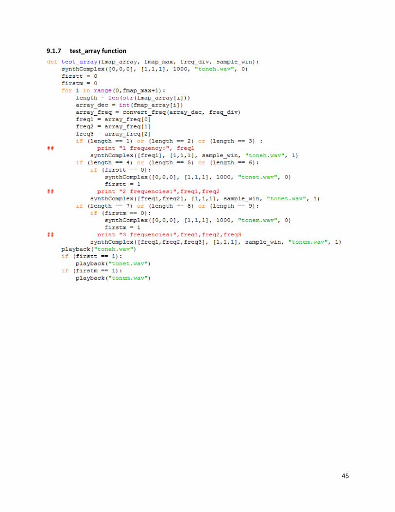
9.1.7 test_array function ............................................................................................................. 45

3

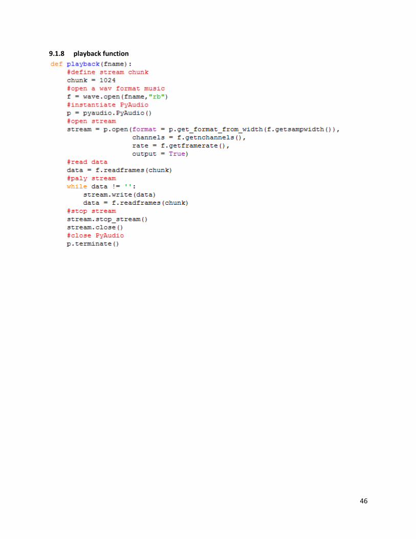
9.1.8 playback function ................................................................................................................ 46

9.1.9 file_to_wave function ......................................................................................................... 47

9.1.10 file_to_freq_array function ................................................................................................. 47

9.1.11 clean_freq function ............................................................................................................. 48

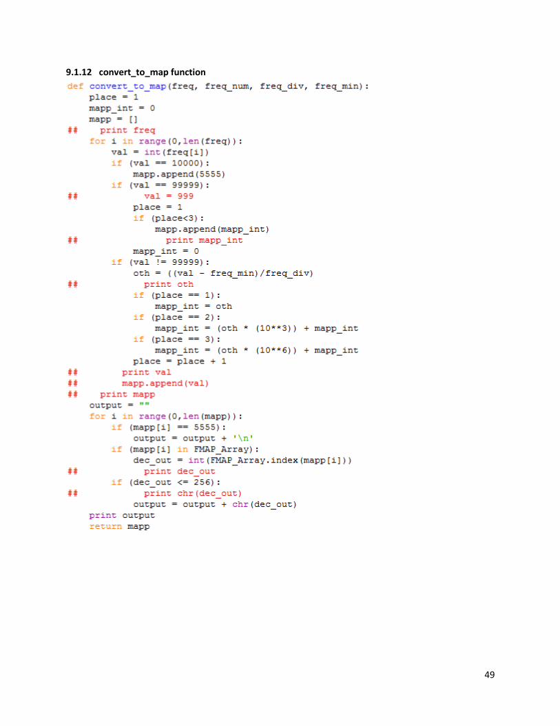
9.1.12 convert_to_map function ................................................................................................... 49

9.1.13 command_arduino function ............................................................................................... 50

9.2 Arduino Code .............................................................................................................................. 50

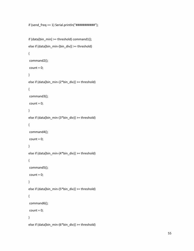
9.2.1 Receiver ............................................................................................................................... 50

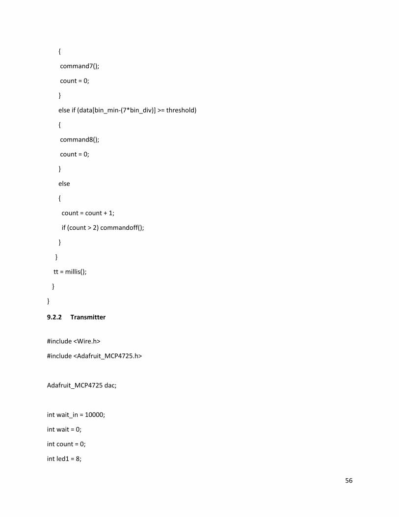
9.2.2 Transmitter ......................................................................................................................... 56

9.2.3 FFT Library ........................................................................................................................... 67

9.3 Permutation Matrix .................................................................................................................... 75

9.4 LabView Virtual Instrument ........................................................................................................ 80

4

2 PREFACE

This project incorporates the material and academic topics covered in the majority of

my coursework here at the Florida Institute of Technology. Much of the signal processing

algorithms, specifically with DFTs, were covered in Digital Signal Processing I (ECE 5245) The

design of the frequency mapping algorithm was accomplished by using techniques learned in

Combinatorics / Graph Theory (MTH 5050). The Arduino software and hardware

implementation methodologies were covered extensively in Mechatronics (MAE 5316). The

control software was developed as a result of ample programming in a Python environment in

Artificial Intelligence/Robotics (CSE 5694). The underwater acoustic design considerations were

a direct result from coursework in Hydroacoustics (OCE 4545). The methodologies for the

design and development of the LabView signal processing software was cultivated in

Instrumentation Design and Scientific Measurement (MAE 5318) and the overall system design

incorporated techniques from Control Systems (MAE 4014). This technical project also reflects

the multi-disciplinary approach that I took to pursue my M.S. in Ocean Engineering by

incorporating aspects from Electrical Engineering, Mechanical Engineering, Computer Science,

and Ocean Engineering.

3 INTRODUCTION

The initial purpose of this technical project was to improve a personal understanding of

both the current communications methods and protocols used in modern acoustic modems as

well as develop a reliable and inexpensive system using off the shelf electronics,

microcontrollers, and single board computers. Acoustic communications are the predominant

method used today for the transfer of data underwater. There are a wide number of

applications such as underwater instrumentation monitoring, controlling and communicating

with various underwater robotic systems such as Remotely Operated Vehicles (ROVs) and

Autonomous Underwater Vehicles (AUVs), and submerged equipment recovery. Currently,

there is a great deal of research into developing a new infrastructure of underwater sensors

networks that communicate oceanographic information in near real time. These networks will

5

allow for quicker detection and analysis of pollution data, tsunami prediction, and

meteorological information. [1] A compact, inexpensive, and reliable device that can

communicate acoustically to buoys and other equipment that are interfaced with satellite

communication systems would be highly desirable for the creation of this network

inexpensively. Initially, the end product of this Technical Project was to develop and design an

underwater communications device that could be interfaced with such a system by using Atmel

microcontrollers, a Raspberry Pi single board computer, and a Laptop computer with LabView

as seen in Figure 1.

However, the implemented communication protocol which I developed, though reliable

in its broadcast and reception, was not sufficiently fast enough to merit its use over traditional

acoustic modem methodologies for large scale data transfers. The project did provide insight

into a novel means by which an inexpensive command and control network could be

implemented for subsea systems where valves, actuators, inflation bags, switching devices, and

6

data collections systems can be controlled from the surface via laptop connected to a

hydrophone and underwater speaker. (See Figure 2)

Figure 2: Unidirectional System

The preferred medium for wireless communication underwater has been sound due to

the highly absorptive properties of seawater with respect to radio waves. Most Radio Wave (RF)

frequencies are completely absorbed by water within only a few meters. There is a logarithmic

relationship, as can be seen in Figure 2, of RF attenuation in seawater. The attenuation factor,

α, in decibels per meter for water is related to the square root of the frequency, f, in hertz [Hz]

multiplied by the conductivity of the water, σ, in Siemens per meter [S/m]. The resulting electric

field, Ex, is an exponential function of the attenuation. [2]

√

7

One can see that the Extremely Low Frequencies (ELF), Super Low Frequencies (SLF),

and Ultra Low Frequencies (ULF) of the order of 1 to 1000 Hz are the only practical frequencies

which can be used for subsea RF communications. Please note that these figures and

calculations only account for the primary losses from radio wave attenuation and do not

account for other additional losses such as those specific to different fluid densities. As a result

of these losses, underwater radio systems require high power and extremely long transmitting

antennae due to their long wavelengths and are therefore impractical for the majority of

underwater communications applications.

Figure 3: Approximate RF Frequency Attenuations in Seawater [2]

There are significant challenges with the signal processing of acoustic communications

that are distinctly different than that of over the air RF communications. First of all, the speed

of sound underwater (~1500 m/s) is significantly slower than that of RF energy (~3x108 m/s)

This slower speed increases the amount of time the data takes to traverse the distance

between a transmitter and receiver yielding the information to be near-real time at best. The

slower speed also results in more pronounced effects such as multipath and Doppler shift (see

Acoustic Communication Design Considerations) not normally encountered in typical RF

communications. Secondly, there is a much lower maximal frequency range (kHz) with

underwater acoustic communications than that of RF (GHz). As can be seen in the Signal

Processing section of this paper, this affects the maximum amount of information that can be

sent per second. Resultantly, the data transfer rates for current acoustic modems are limited to

a maximum of 115kbps. This Technical Project investigates these limitations through an

independent experimental development of an alternative communications protocol.

8

4 UNDERWATER ACOUSTICS HISTORY [3]

Underwater acoustic properties have been known by man for over two millennia.

However, the majority of modern day investigations into the subject have been undertaken in

the last two hundred years. In the mid-300s B.C. Aristotle noted that sound could be heard in

water as good as in air. Nearly eighteen hundred years later, Leonardo DaVinci observed that

ships could be heard at great distances underwater. In the 1620s, Marin Mersenne published

“L’Harmonie Universelle” in which he described his experiments with sound and experimental

measurements of its speed. This is the first book of record in modern times that was published

on the subject of hydroacoustics.

Figure 4: Excerpt from “L’Harmonie Universelle” [4]

Sixty years later, a more formalized mathematical representation of sound propagation could

be found in Sir Isaac Newton’s “Philosphiae Naturalis Principia Mathematica.” Building off of

the work of Newton, Abbé J.A. Nollet later performed a series of experiments in 1743 that

proved sound could indeed travel underwater.

An accurate measure of sound velocities underwater was performed through a series of

experiments by different scientists throughout the 1800s. In 1820, Froncois Sulpice Beudant

9

measured the speed of sound in the ocean near Marseilles as being 1500 m/s. Jean-Daniel

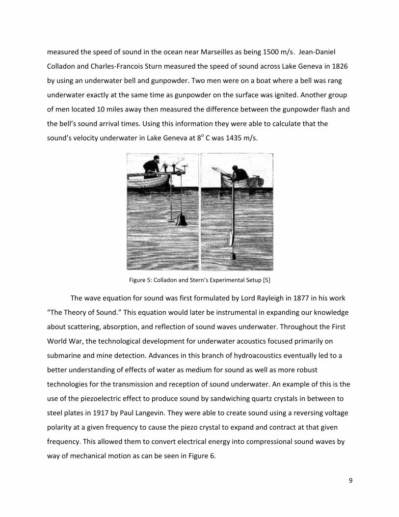
Colladon and Charles-Francois Sturn measured the speed of sound across Lake Geneva in 1826

by using an underwater bell and gunpowder. Two men were on a boat where a bell was rang

underwater exactly at the same time as gunpowder on the surface was ignited. Another group

of men located 10 miles away then measured the difference between the gunpowder flash and

the bell’s sound arrival times. Using this information they were able to calculate that the

sound’s velocity underwater in Lake Geneva at 8o C was 1435 m/s.

Figure 5: Colladon and Stern’s Experimental Setup [5]

The wave equation for sound was first formulated by Lord Rayleigh in 1877 in his work

“The Theory of Sound.” This equation would later be instrumental in expanding our knowledge

about scattering, absorption, and reflection of sound waves underwater. Throughout the First

World War, the technological development for underwater acoustics focused primarily on

submarine and mine detection. Advances in this branch of hydroacoustics eventually led to a

better understanding of effects of water as medium for sound as well as more robust

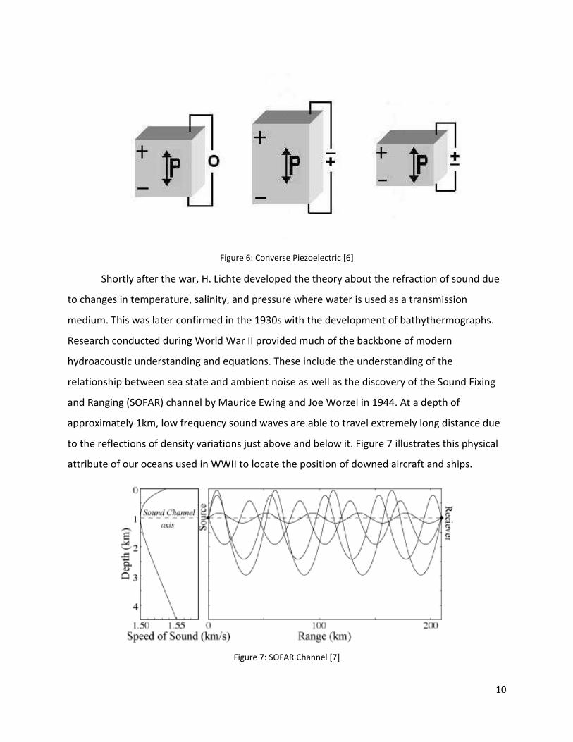
technologies for the transmission and reception of sound underwater. An example of this is the

use of the piezoelectric effect to produce sound by sandwiching quartz crystals in between to

steel plates in 1917 by Paul Langevin. They were able to create sound using a reversing voltage

polarity at a given frequency to cause the piezo crystal to expand and contract at that given

frequency. This allowed them to convert electrical energy into compressional sound waves by

way of mechanical motion as can be seen in Figure 6.

10

Figure 6: Converse Piezoelectric [6]

Shortly after the war, H. Lichte developed the theory about the refraction of sound due

to changes in temperature, salinity, and pressure where water is used as a transmission

medium. This was later confirmed in the 1930s with the development of bathythermographs.

Research conducted during World War II provided much of the backbone of modern

hydroacoustic understanding and equations. These include the understanding of the

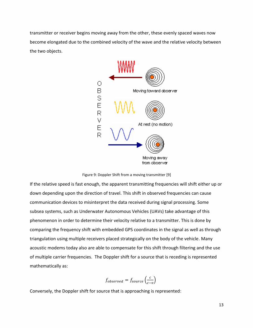
relationship between sea state and ambient noise as well as the discovery of the Sound Fixing

and Ranging (SOFAR) channel by Maurice Ewing and Joe Worzel in 1944. At a depth of

approximately 1km, low frequency sound waves are able to travel extremely long distance due

to the reflections of density variations just above and below it. Figure 7 illustrates this physical

attribute of our oceans used in WWII to locate the position of downed aircraft and ships.

Figure 7: SOFAR Channel [7]

11

Advances in technology continue today. A great deal of research has been devoted to

increasing bandwidth and data transfer rates as more advanced subsea devices are put in to

use in our oceans.

5 ACOUSTIC COMMUNICATIONS DESIGN CONSIDERATIONS

5.1 FREQUENCY ATTENUATION

The attenuation of an acoustic signal in water depends primarily on the frequency of the

signal. This is due to the conversion of the mechanical and compressive energy of the acoustic

signal into thermal energy by the vibration of the molecules used as a transmission medium. In

the case of seawater, the density of the medium can vary depending upon the salinity,

pressure, and temperature of the water. This means that different layers of the ocean can

attenuate certain frequencies greater than others. In general, higher frequencies tend to be

absorbed at a greater magnitude than that of lower frequencies. Additionally attenuation also

occurs from spreading loss. Spreading loss results from the geometric distribution of the

compressive mechanical energy from the transmitting source. (See Figure 8) This type of loss is

frequently modeled as spherical at short distances and cylindrical at long distances because of

the relative geometric change once the signal reaches the surface and seafloor.

Figure 8: Spherical and Cylindrical Spreading Loss [9]

12

Both of these losses act in effect as part of the frequency response of the system or medium by

which the signal is transmitted over. For frequencies under 50 kHz as in this project, these

attenuated losses ( ) can be expressed using the following equation [8]:

( ) (

)

( )

Where,

( )

The absorption coefficient is defined as ( ) where f is frequency. The transmission distance, ,

is determine in reference to distance, . The spreading loss is modeled with k which equal to 1

if the spreading loss is cylindrical and 2 if it is spherical. The calculated attenuation value in

conjunction with ambient noise. N, present in the medium and the spectral power density, S, of

the transmitter is used to determine the signal to noise ratio, SNR, as can be seen in the

following equation [8]:

( )

( ) ( )⁄

These equations are useful in determining a rough estimate of the range of the transmitter

given a known power output and spectral density. Variations in density of the ocean at various

depths and salinities do not however make it an exact science. The device designed in this

project uses relatively low frequencies and its primary function is for communications at

distances of 500 meters or less. Its operating parameters are therefore well within these

constraints given acceptable and realistic transmission power requirements.

5.2 DOPPLER SHIFT

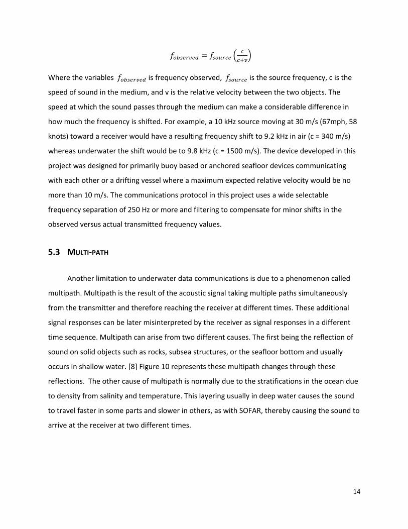
An additional consideration when designing acoustic communication systems is the

Doppler shift. This shift is due to the compression and elongation of waves by a moving object.

As can be seen with the example in Figure 9, a transmitting object that is not moving relative to

its receiver has evenly spaced wavelengths over the whole of its geometry. Once either the

13

transmitter or receiver begins moving away from the other, these evenly spaced waves now

become elongated due to the combined velocity of the wave and the relative velocity between

the two objects.

Figure 9: Doppler Shift from a moving transmitter [9]

If the relative speed is fast enough, the apparent transmitting frequencies will shift either up or

down depending upon the direction of travel. This shift in observed frequencies can cause

communication devices to misinterpret the data received during signal processing. Some

subsea systems, such as Underwater Autonomous Vehicles (UAVs) take advantage of this

phenomenon in order to determine their velocity relative to a transmitter. This is done by

comparing the frequency shift with embedded GPS coordinates in the signal as well as through

triangulation using multiple receivers placed strategically on the body of the vehicle. Many

acoustic modems today also are able to compensate for this shift through filtering and the use

of multiple carrier frequencies. The Doppler shift for a source that is receding is represented

mathematically as:

(

)

Conversely, the Doppler shift for source that is approaching is represented:

14

(

)

Where the variables is frequency observed, is the source frequency, c is the

speed of sound in the medium, and v is the relative velocity between the two objects. The

speed at which the sound passes through the medium can make a considerable difference in

how much the frequency is shifted. For example, a 10 kHz source moving at 30 m/s (67mph, 58

knots) toward a receiver would have a resulting frequency shift to 9.2 kHz in air (c = 340 m/s)

whereas underwater the shift would be to 9.8 kHz (c = 1500 m/s). The device developed in this

project was designed for primarily buoy based or anchored seafloor devices communicating

with each other or a drifting vessel where a maximum expected relative velocity would be no

more than 10 m/s. The communications protocol in this project uses a wide selectable

frequency separation of 250 Hz or more and filtering to compensate for minor shifts in the

observed versus actual transmitted frequency values.

5.3 MULTI-PATH

Another limitation to underwater data communications is due to a phenomenon called

multipath. Multipath is the result of the acoustic signal taking multiple paths simultaneously

from the transmitter and therefore reaching the receiver at different times. These additional

signal responses can be later misinterpreted by the receiver as signal responses in a different

time sequence. Multipath can arise from two different causes. The first being the reflection of

sound on solid objects such as rocks, subsea structures, or the seafloor bottom and usually

occurs in shallow water. [8] Figure 10 represents these multipath changes through these

reflections. The other cause of multipath is normally due to the stratifications in the ocean due

to density from salinity and temperature. This layering usually in deep water causes the sound

to travel faster in some parts and slower in others, as with SOFAR, thereby causing the sound to

arrive at the receiver at two different times.

15

Figure 10: Multipath Signal Distortion [7]

The multipath signal in shallow water is normally easier to model due to its uniform density.

The speed of sound remains constant as a result of this uniform density and therefore its time

delay is a linear function of sound velocity divided by the total distance traveled. Additionally,

the gain of this system decreases linearly with this increased distance as a function of the

frequency. However, changes in density as seen in a deep water environment, affect the speed

of the signal and hence the signal’s phase. It also can affect the gain of the signal differently

with no clear linear pattern. Overcoming these challenges requires the system to compensate

for these phase and gain changes by being able to both capture the frequency response of each

path and filter out path frequency responses that are asynchronous with the communication

signal. Milica Stonjanovic quantifies these variations in multipath frequency response and

impulse response through the use of the following equations in “Underwater Acoustic

Communications: Design Considerations on the Physical Layer” [8]. and are the

frequency response and impulse response respectively for each path, p, at a given frequency, f:

( ) ∑ ( )

16

( ) ∑ ( )

The variable is the time for the signal to reach the receiver for each path and ( ) is the

inverse Fourier transform of ( ). For the purposes this project, multipath was overcome

through longer transmit times. It was determined experimentally, that the system had poor

frequency separation at shorter transmit time intervals, therefore a greater number of

frequencies were used with a longer transmit time in order to balance the density of data per

second.

6 SIGNAL PROCESSING

An integral portion of the functionality of this project’s communication protocols

required an analysis of the frequency spectrum of an acoustic signal measured in the time

domain. This conversion was accomplished through the use a Fast Fourier Transform (FFT). In

order to understand an FFT works, one must first understand the Continuous Fourier Transform

and its digital version, the Discrete Fourier Transform.

6.1 FOURIER TRANSFORM

In 1822, Joseph Fourier published “Theorie analytique de la chaleur” where he

introduced the idea that nearly every function can be described as a summation of sine and

cosine functions with different weights and frequencies as seen in the equation below. This

equation is known as the Fourier series [10].

( ) ∑( )

17

This equation can also be modified to describe a periodic function of x over discrete distances

– and . [10]

( ) ∑(

)

Where the coefficients are defined,

∫ ( )

∫ ( )

Normally, periodic signals or waveforms that are analyzed for signal processing are taken over

the time domain where ( ) is a function of time rather than some distance x. The sampling

window of the periodic function now becomes –t0 to t0. The Fourier series for the periodic

function in time domain therefore come to be:

( ) ∑(

)

Where,

∫ ( )

∫ ( )

Much of signal processing also involves the complex plane. This is due to primarily to phase

shifts that take place on an analog signal as a result of the system’s physical characteristics. For

example, suppose one were to inject a sine wave voltage into three different circuits: One with

a resistor, one with an inductor, and one with a capacitor as seen in Figure 11. The measured

current of the resistive circuit A would have the same phase as that of the voltage. The

18

measured currents, however, of inductive and capacitive circuits B and C would be shifted 90o

negatively and positively respectively.

Figure 11: Phase response of a resistor, inductor, and capacitor [11]

This phase shifts are best represented mathematically over the complex plane. Therefore the

ideal Fourier series for use in signal processing is the complex Fourier series where the

coefficient sine component is an imaginary number . The series then takes the form:

( ) ∑

⁄

Where,

∫ ( )

⁄

This series represents the time dependent function ( ) as a combination of circles on the

complex plane. If we want to express those values and find the transformation to the frequency

domain we must first identify that the limits or window of the periodic function as defined by t0

can be expressed as a frequency ω0 through the relationship:

19

Through the substitution of cn into the Fourier series with some careful Calculus and Algebra as

seen on page 846 Donald A. McQuarrie’s “Mathematical Methods for Scientists and Engineers”

[10] we are able to arrive to the inverse Fourier transform:

( )

√ ∫ ( )

Where ( ) is the function of ( ) represented in the frequency domain. Inversely, the Fourier

transform can be used to map the time domain function ( ) over the frequency domain:

( )

√ ∫ ( )

This mathematical property allows us to solve both ordinary and partial differential equations

by analyzing time dependent functions in the frequency domain. For signal processing, this

gives us a bridge between the time domain and frequency domain of signal which allows one to

model the characteristics of the system that signal goes through. The calculated or measured

frequency response of the system, ( ), can be convolved with the input signal ( ) to find

and predict the effects of the system on the output ( ). These functions in the frequency

domain can then be returned time domain through the use of the Inverse Fourier Transform.

This project uses the Fourier Transform to determine the component frequencies of the

transmitted signals and also can be used to test the acoustic frequency response of various

underwater systems. The LabView Virtual Instrument in this project was developed specifically

for the purpose of signal analysis of a given transmitting medium.

6.2 DISCRETE FOURIER TRANSFORM (DFT)

One design limitation to this project is the fact that the acoustic signals could not be

measured continuously due to the non-continuous nature of digital electronics. Discrete

amplified analog voltages sampled at regular pre-determined intervals were taken from the

microphones and converted into arrays of digital representations. The conversion of these

discrete samples over time must be done using a discrete Fourier transform, or DFT for short. A

variation of the Fourier transform, known as the discrete time Fourier transform (DTFT), is

20

nearly identical to the Fourier transform with the samples ( ) are mapped over the imaginary

plane through summation rather than integration.

( ) ∑ ( )

The resulting ( ) is the representative frequency component of multiple values of ( ).

Also it is important to notice that is used instead of for the imaginary. This notation is typical

in signal processing and electrical engineering in order to avoid confusion with the current .

The DTFT is not practical for this application due to assumption that an infinite or continuous

number of samples ( ) will be taken. The device designed in this project only processes

discrete windows of N samples and therefore requires the DFT. The DFT is a combination of

Fourier transform of a periodic signal and the DTFT [12]:

( ) ∑ ( )

⁄

Conversely, the inverse DFT can be written as:

( )

∑ ( )

⁄

The notation of the DFT is often simplified by defining:

⁄

The DFT is typically therefore written:

( ) ∑ ( )

21

6.3 FAST FOURIER TRANSFORM (FFT)

The conversion of a time domain based array of samples into an array of magnitudes for a

correlating frequency component of the captured signal requires an extensive number of

computations by the computer processor when using the DFT. For larger processors the speed

is sufficient to make these calculations fast enough so that the data is transformed fast enough

for hardware integration. However, when using a smaller processor on microcontrollers like the

Arduino Uno, a more efficient algorithm is required. This is accomplished through the use of the

Fast Fourier Transform (FFT). The FFT takes advantage of the symmetry in order to minimize the

total number of calculations undertaken by the processor. There are many different FFT

algorithms that are in use today. The FFT used in this project was an open source FFT that used

a decimation-in-time radix-2 algorithm. This algorithm splits the captured time domain signal

into even and odd indexed terms and then exploits repetitious calculations through a butterfly

pattern where at each node a varying twiddle factor W weights the indexed term.

Figure 12: Eight point radix-2 decimation in time FFT

22

7 PROJECT DESIGN

7.1 THEORY

7.1.1 Motivation

The motivation behind this project and resulting technical report was to design, build,

and test a system that transmits and receives data acoustically through spaced frequencies as

chords representing Boolean table values. The device’s eventual intended use is for the wireless

control and actuation of various mechatronic devices underwater and/or the collection of data

from subsea instrumentation. The transmitted chord of frequencies represents a command that

is sent to an underwater device. For example, a four frequency system at 1 kHz, 2 kHz, 3 kHz,

and 4 kHz would represent a four bit binary number. Should all four frequencies be transmitted

as a chord simultaneously, the resulting binary representation of the signal would be 1111.

Similarly, if only 1 kHz and 3 kHz signals were transmitted as a chord the resulting binary

representation would be 0101. Therefore a four bit four frequency signal would correlate to 15

possible command variations. The receiver would determine the frequencies transmitted

through the use of a FFT and then correlate those frequencies to the binary command

sequence that was issued by the transmitter through the use of a table. Below is an example

table of command sequences:

Table 1: Example system command byte correlation

23

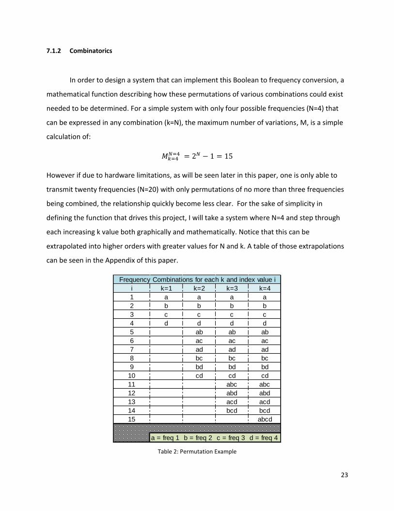
7.1.2 Combinatorics

In order to design a system that can implement this Boolean to frequency conversion, a

mathematical function describing how these permutations of various combinations could exist

needed to be determined. For a simple system with only four possible frequencies (N=4) that

can be expressed in any combination (k=N), the maximum number of variations, M, is a simple

calculation of:

However if due to hardware limitations, as will be seen later in this paper, one is only able to

transmit twenty frequencies (N=20) with only permutations of no more than three frequencies

being combined, the relationship quickly become less clear. For the sake of simplicity in

defining the function that drives this project, I will take a system where N=4 and step through

each increasing k value both graphically and mathematically. Notice that this can be

extrapolated into higher orders with greater values for N and k. A table of those extrapolations

can be seen in the Appendix of this paper.

Table 2: Permutation Example

i k=1 k=2 k=3 k=4

1 a a a a

2 b b b b

3 c c c c

4 d d d d

5 ab ab ab

6 ac ac ac

7 ad ad ad

8 bc bc bc

9 bd bd bd

10 cd cd cd

11 abc abc

12 abd abd

13 acd acd

14 bcd bcd

15 abcd

a = freq 1 b = freq 2 c = freq 3 d = freq 4

Frequency Combinations for each k and index value i

24

Notice that for a k value of 1, the maximum number of permutations is exactly equal to the

number of frequencies. This should be intuitive as only one frequency can be transmitted at a

time when k=1.

Now if k is increased to 2, the maximum number of permutations becomes the summation of

all positive integers over N.

∑

Increasing k to 3 appears to complicate things even further:

∑∑

However, analyzing a table of calculated M from N and k shows that a clear pattern exists:

Table 3: Extrapolated Values for Maximum Variation M

The maximum number of permutations can be written as a function of previous maximum

permutation values for a system with one less frequency:

This relationship between other maximum permutation calculations allows the calculation of

larger systems without requiring increased processing time for large nested summations.

1 2 3 4 5 6 7 8 9 10

2 1 3 6 10 15 21 28 36 45 55

3 1 3 7 14 25 41 63 92 129 175

4 1 3 7 15 30 56 98 162 255 385

5 1 3 7 15 31 62 119 218 381 637

6 1 3 7 15 31 63 126 246 465 847

7 1 3 7 15 31 63 127 254 501 967

8 1 3 7 15 31 63 127 255 510 1012

9 1 3 7 15 31 63 127 255 511 1022

10 1 3 7 15 31 63 127 255 511 1023

Number of Frequencies (N)

Perm

uta

tion V

alu

e (

k)

25

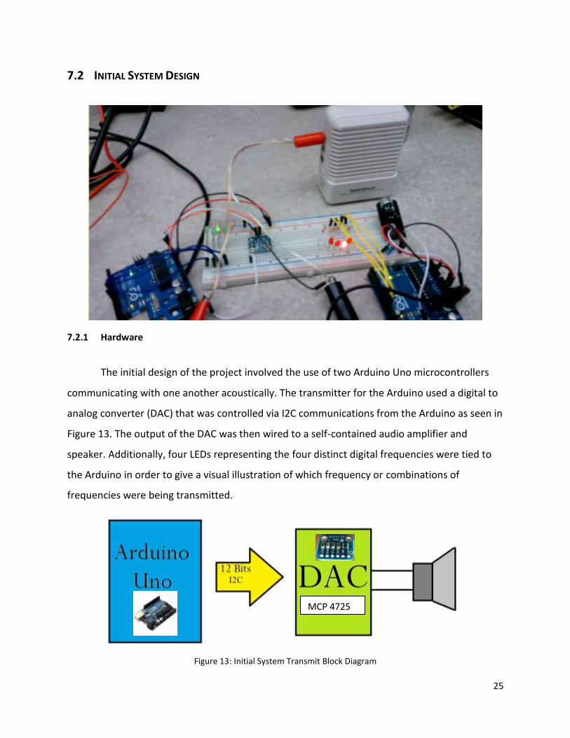
7.2 INITIAL SYSTEM DESIGN

7.2.1 Hardware

The initial design of the project involved the use of two Arduino Uno microcontrollers

communicating with one another acoustically. The transmitter for the Arduino used a digital to

analog converter (DAC) that was controlled via I2C communications from the Arduino as seen in

Figure 13. The output of the DAC was then wired to a self-contained audio amplifier and

speaker. Additionally, four LEDs representing the four distinct digital frequencies were tied to

the Arduino in order to give a visual illustration of which frequency or combinations of

frequencies were being transmitted.

Figure 13: Initial System Transmit Block Diagram

MCP 4725

26

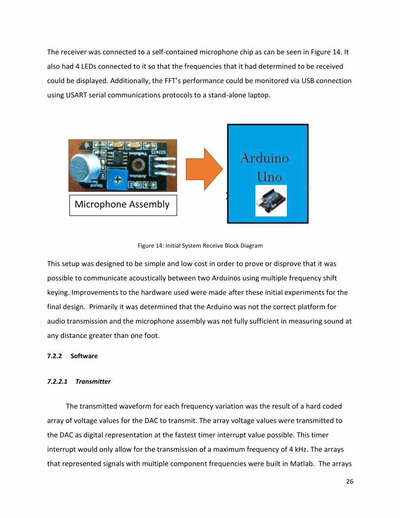
The receiver was connected to a self-contained microphone chip as can be seen in Figure 14. It

also had 4 LEDs connected to it so that the frequencies that it had determined to be received

could be displayed. Additionally, the FFT’s performance could be monitored via USB connection

using USART serial communications protocols to a stand-alone laptop.

Figure 14: Initial System Receive Block Diagram

This setup was designed to be simple and low cost in order to prove or disprove that it was

possible to communicate acoustically between two Arduinos using multiple frequency shift

keying. Improvements to the hardware used were made after these initial experiments for the

final design. Primarily it was determined that the Arduino was not the correct platform for

audio transmission and the microphone assembly was not fully sufficient in measuring sound at

any distance greater than one foot.

7.2.2 Software

7.2.2.1 Transmitter

The transmitted waveform for each frequency variation was the result of a hard coded

array of voltage values for the DAC to transmit. The array voltage values were transmitted to

the DAC as digital representation at the fastest timer interrupt value possible. This timer

interrupt would only allow for the transmission of a maximum frequency of 4 kHz. The arrays

that represented signals with multiple component frequencies were built in Matlab. The arrays

Microphone Assembly

27

were then hardcoded in order to conserve processing power for the I2C communications. Had

the output voltage been calculated by using a sine function of the time in the timer interrupt

clock with the desired frequency, the processor would have been slowed down considerably.

Unfortunately even with these hard-coded arrays, this system performed extremely poorly due

to the distortion from the lagged voltage response of the DAC. Additionally, only a limited

number of arrays could be stored due to limitations of memory on the Arduino.

7.2.2.2 Receiver

The receiver software would simply poll the analog input pin at specific timer interrupts

in order to measure the voltage level. This voltage level would then be stored as a value in an

array. Once enough array samples were taken, the timer interrupt would stop. The FFT function

would be then called and an array of frequency bins would be returned. The software then

compared the bins of the desired frequencies to see if their threshold was high enough for it to

be a component frequency.

Figure 15: Arduino Receiver Algorithm

This FFT worked great on the Arduino as long as no more than 3 frequencies were combined

simultaneously. The overlaps of spectrums of closely related chords at 3 frequencies caused

severe issues for the device in the discernment of the command issued.

Array of

Samples Taken

FFT Performed

on Array FFT O/P Array

Converted into

Component

Frequencies

28

7.3 IMPROVED SYSTEM DESIGN

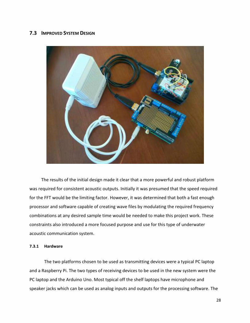
The results of the initial design made it clear that a more powerful and robust platform

was required for consistent acoustic outputs. Initially it was presumed that the speed required

for the FFT would be the limiting factor. However, it was determined that both a fast enough

processor and software capable of creating wave files by modulating the required frequency

combinations at any desired sample time would be needed to make this project work. These

constraints also introduced a more focused purpose and use for this type of underwater

acoustic communication system.

7.3.1 Hardware

The two platforms chosen to be used as transmitting devices were a typical PC laptop

and a Raspberry Pi. The two types of receiving devices to be used in the new system were the

PC laptop and the Arduino Uno. Most typical off the shelf laptops have microphone and

speaker jacks which can be used as analog inputs and outputs for the processing software. The

29

Raspberry Pi also comes equipped with an audio output jack for easy integration with an

underwater speaker. The Pi, however, does not have any analog inputs and therefore requires

the integration of an Arduino Uno for bi-directional communication to take place. The laptop

interface is designed for onshore or shipboard communication with remote subsea devices.

One application for the laptop is to send a broadcast signal to slave Arduino Uno’s controlling

either electronic or electro-mechanical devices such as valves, telecommunication switches, or

actuating inflatable lift bags for subsea instrumentation and equipment.

Figure 16: Applications of System Design

Another application for this system is the bidirectional communication with a Raspberry Pi link

via USB with an Arduino Uno. The laptop could issue a command for the Pi to transmit the

result of the data it has collected over the past week. As can be seen in the software section of

this report, the Laptop then converts the return acoustic transmission from the Pi into a text

file. Additionally, the system has the capability to issue a command to the Pi to transmit various

combinations of frequencies in a predictive manner so that the frequency response of the

medium in which the communication is taking place can be measured.

Laptop

Arduino

Uno

Laptop Laptop

Raspberry Pi

Arduino

Uno

Arduino

Uno

Arduino

Uno

30

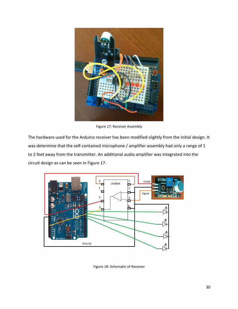
Figure 17: Receiver Assembly

The hardware used for the Arduino receiver has been modified slightly from the initial design. It

was determine that the self-contained microphone / amplifier assembly had only a range of 1

to 2 feet away from the transmitter. An additional audio amplifier was integrated into the

circuit design as can be seen in Figure 17.

Figure 18: Schematic of Receiver

31

This additional amplifier provided much better range as well as improved frequency

discrimination by the FFT.

7.3.2 Software

7.3.2.1 Laptop

The laptop incorporates the use of two separate programs running simultaneously with

one another while sharing a common text file and therefore was designed into two parts. The

signal processing of a received signal is done initially through the LabView Virtual Instrument I

developed. The instrument records acoustic data taken from the microphone jack on the laptop

via a subVI acquired online [14] and coverts it into an array.

Figure 19: LabView Virtual Instrument Signal Processing

This data is then processed via FFT and the spectral frequencies of the signals are then

displayed graphically at the user interface.

32

Figure 20: LabView Virtual Instrument User Interface

These values are then further filtered and conditioned into a usable collection of frequencies.

These frequencies are then recorded onto a log file which is then processed by the other

software. At the heart of this system’s design is the encoding, decoding, and transmitting

software. This software was written in Python due to its ease of incorporation into both a PC

Windows Operating System and the Linux based Debian Operating System for the Raspberry Pi.

Python also has a vast number of open source libraries for serial communications, construction

of wave files, and array manipulation. Most importantly, it is light enough to operate on a Pi

with less lag than that of C++. The main control software is composed of three parts: frequency

array mapping, byte to frequency encoding, wave file creation and playback, frequency to byte

decoding, and text file to byte conversion.

7.3.2.1.1 Frequency Array Mapping

Figure 21: Frequency Mapping Logic

Calculate

Array Size

Map

Frequency

Tags to

Array

k

N

33

The frequency array mapping function is the heart to this system. It is the function that

provides a map by which frequencies combinations are attributed to a decimal value. The

function builds a map from two inputs which are N and k. N is total the number desired

frequencies to be used in the system and k is maximum number of frequencies that can be

combined into one signal. The function first determines the maximum number of combinations

given N and k and then maps every permutation as an encoded integer value to a decimal index

term.

Table 4: Array Values for N=3 and k=3

The frequencies are spaced such that the maximum allowable N value is 999. For the purposes

of this project only 20 frequencies (N=20) with a maximum combination of 3 (k=3) were used.

The mathematical relationships of how the number of possible permutations can be calculated

are discussed in the section 8.1.2 of this paper. Additionally, a table showing that maximum

value for any set of k and N can be seen in the Appendix.

A[0] 000 000 000

A[1] 000 000 001

A[2] 000 000 002

A[3] 000 000 003

A[4] 000 002 001

A[5] 000 003 001

A[6] 000 003 002

k=3 A[7] 003 002 001

N = 3

k = 1

k = 2

34

7.3.2.1.2 User Interface

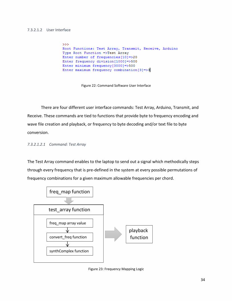
Figure 22: Command Software User Interface

There are four different user interface commands: Test Array, Arduino, Transmit, and

Receive. These commands are tied to functions that provide byte to frequency encoding and

wave file creation and playback, or frequency to byte decoding and/or text file to byte

conversion.

7.3.2.1.2.1 Command: Test Array

The Test Array command enables to the laptop to send out a signal which methodically steps

through every frequency that is pre-defined in the system at every possible permutations of

frequency combinations for a given maximum allowable frequencies per chord.

Figure 23: Frequency Mapping Logic

freq_map function

test_array function

freq_map array value

convert_freq function

synthComplex function

playback

function

35

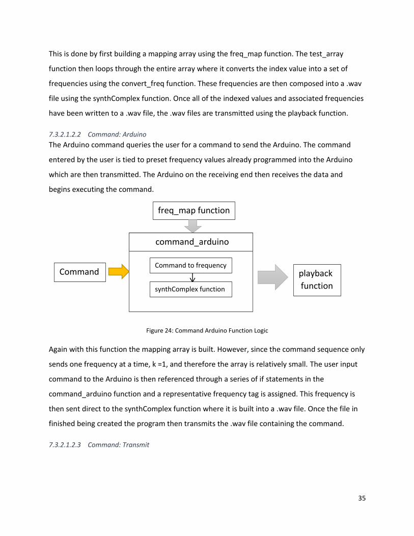
This is done by first building a mapping array using the freq_map function. The test_array

function then loops through the entire array where it converts the index value into a set of

frequencies using the convert_freq function. These frequencies are then composed into a .wav

file using the synthComplex function. Once all of the indexed values and associated frequencies

have been written to a .wav file, the .wav files are transmitted using the playback function.

7.3.2.1.2.2 Command: Arduino

The Arduino command queries the user for a command to send the Arduino. The command

entered by the user is tied to preset frequency values already programmed into the Arduino

which are then transmitted. The Arduino on the receiving end then receives the data and

begins executing the command.

Figure 24: Command Arduino Function Logic

Again with this function the mapping array is built. However, since the command sequence only

sends one frequency at a time, k =1, and therefore the array is relatively small. The user input

command to the Arduino is then referenced through a series of if statements in the

command_arduino function and a representative frequency tag is assigned. This frequency is

then sent direct to the synthComplex function where it is built into a .wav file. Once the file in

finished being created the program then transmits the .wav file containing the command.

7.3.2.1.2.3 Command: Transmit

freq_map function

playback

function

Command

command_arduino

function Command to frequency


36

The transmit command is used to convert a text file into a wave file and then transmit to a

receiving device.

Figure 25: Transmit Command Logic

The transmit command also first builds an array of frequency value using the freq_map. The

current default setting for this function is N=20 and k=3. The file_to_wave function is then

called which systematically reads each line of text from the text file, converts each character

into hex then decimal, references the frequency values for that decimal index, and sends the

corresponding frequency values to the synthComplex function where it is converted into a .wav

file. Once, the function has fully converted the document to .wav file, the playback function is

then called in order to transmit the data.

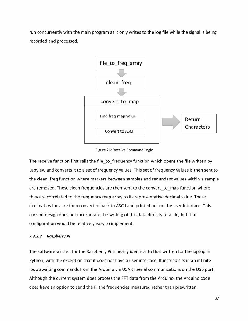
7.3.2.1.2.4 Command: Receive

This command reads a software specific log file written either by Labview which contains

frequency values from a received signal. The incoming acoustic signal should have already been

recorded and processed by the Labview software before this command is given. Labview can

freq_map function


convert_freq function

Find freq_map value

Convert to decimal

Read text from the file

file_to_wave function

playback

function Text File

37

run concurrently with the main program as it only writes to the log file while the signal is being

recorded and processed.

Figure 26: Receive Command Logic

The receive function first calls the file_to_frequency function which opens the file written by

Labview and converts it to a set of frequency values. This set of frequency values is then sent to

the clean_freq function where markers between samples and redundant values within a sample

are removed. These clean frequencies are then sent to the convert_to_map function where

they are correlated to the frequency map array to its representative decimal value. These

decimals values are then converted back to ASCII and printed out on the user interface. This

current design does not incorporate the writing of this data directly to a file, but that

configuration would be relatively easy to implement.

7.3.2.2 Raspberry Pi

The software written for the Raspberry Pi is nearly identical to that written for the laptop in

Python, with the exception that it does not have a user interface. It instead sits in an infinite

loop awaiting commands from the Arduino via USART serial communications on the USB port.

Although the current system does process the FFT data from the Arduino, the Arduino code

does have an option to send the Pi the frequencies measured rather than prewritten

file_to_freq_array

clean_freq

convert_to_map

Find freq map value

Convert to ASCII

Return

Characters

38

commands hard-coded in the Arduino. For demonstration purposes the receiving Arduino was

set in command mode. The software written for the Arduino Uno in the improved system

design is nearly identical to the initial system design with the exception of its built in frequency

to command conversion functions. Minor improvements were also made to the frequency

discrimination of the FFT output that allowed for a smoother response to received command

transmissions.

8 REFERENCES

[1] "Researchers Developing 'Underwater Internet'" PCMAG. N.p., n.d. Web. 15 Jan. 2014

[2] Claus, John. “Attenuation of Electromagnetic Waves in Seawater.” OCN 5401 Term Paper,

Florida Institute of Technology, Dec 2012

[3] "DOSITS: History of Underwater Acoustics." DOSITS: History of Underwater Acoustics. N.p.,

n.d. Web. 11 Feb. 2014.

[4] "Masoneria En Valencia." Masoneria En Valencia. N.p., n.d. Web. 3 Mar. 2014.

[5] Colladon, Daniel. Souvenirs Et M moires Autobiographie. en ve: Impr. Aubert-

Schuchardt, 1893. Print J. D. Colladon, Souvenirs et Memoires, Albert-Schuchardt, Geneva, 1893

[6] "An Introduction to Transducer Crystals." An Introduction to Transducer Crystals. N.p., n.d.

Web. 12 Feb. 2014.

[7] Sing, A.c., J.k. Nelson, and S.s. Kozat. "Signal Processing for Underwater Acoustic

Communications." IEEE Communications Magazine 47.1 (2009): 90-96. Print

[8] Stojanovic , Milica. “Underwater Acoustic Communications: Design Considerations on the

Physical Layer.” Massachusetts Institute of Technology, Cambridge, MA

[9] "Observation Methods." Methods. N.p., n.d. Web. 15 Mar. 2014.

[9] "DOSITS: Cylindrical vs. Spherical Spreading." DOSITS: Cylindrical vs. Spherical Spreading.

N.p., n.d. Web. 15 Mar. 2014

[10] McQuarrie, Donald A. Mathematical Methods for Scientists and Engineers. Sausalito, CA:

University Science, 2003. Print.

[11] "A Level Physics Notes - Electricity - Phase Differences Between Current and Voltage for

Resistors, Capacitors and Inductors." A Level Physics Notes - Electricity - Phase Differences

39

Between Current and Voltage for Resistors, Capacitors and Inductors. N.p., n.d. Web. 18 Mar.

2014.

[12] Oppenheim, Alan V., and Ronald W. Schafer. Discrete-time Signal Processing. London:

Prentice-Hall, 1989. Print.

9 APPENDICES

9.1 PYTHON CODE

9.1.1 Shared Main

40

9.1.2 Laptop Main

41

9.1.3 Raspberry Pi Main

42

9.1.4 freq_map function

43

9.1.5 synthComplex function

44

9.1.6 convert_freq function

45

9.1.7 test_array function

46

9.1.8 playback function

47

9.1.9 file_to_wave function

9.1.10 file_to_freq_array function

48

9.1.11 clean_freq function

49

9.1.12 convert_to_map function

50

9.1.13 command_arduino function

9.2 ARDUINO CODE

9.2.1 Receiver

#include "fix_fft.h"

char im[256];

char data[256];

float freq_min = 500;

float freq_div = 1000;

int send_freq = 0;

int bin = 0;

51

int bin_min;

int bin_div;

int count = 0;

int freq = 0;

int threshold = 5;

void command1(){

if (send_freq == 0) Serial.println("command1");

digitalWrite(8, HIGH);

digitalWrite(9, LOW);



}

void command2(){






}

void command3(){






}

void command4(){

52






}

void command5(){






}

void command6(){






}

void command7(){






}

void command8(){


53





}

void commandoff(){

if (send_freq == 0) Serial.println("commandoff");





}

void setup(){

Serial.begin(9600);

pinMode(8, OUTPUT);

pinMode(9, OUTPUT);

pinMode(10, OUTPUT);

pinMode(11, OUTPUT);

bin_min = int(((-0.003)*freq_min)+63.5);

bin_div = int(freq_div/333);

Serial.println(bin_min);

Serial.println(bin_div);

}

void loop(){

54

int static i = 0;

static long tt;

int val;

if (millis() > tt){

if (i < 128){

val = analogRead(1)*2 -128;

//Serial.print(val);

//Serial.print(" ");

data[i] = val;

im[i] = 0;

i++;

}

else{

fix_fft(data,im,7,0);

for (i=0; i< 64;i++){

//Serial.print(data[i], DEC);


data[i] = sqrt(data[i] * data[i] + im[i] * im[i]);

//if (data[i] > threshold)

//Serial.print(i,DEC);

//Serial.print(data[i], DEC);


if (send_freq == 1)

{

if (data[i] > threshold)

freq = int((-333.33*i)+21166.7);

Serial.println(freq);

}

}

55

if (send_freq == 1) Serial.println("###########");

if (data[bin_min] >= threshold) command1();

else if (data[bin_min-(bin_div)] >= threshold)

{

command2();

count = 0;

}

else if (data[bin_min-(2*bin_div)] >= threshold)

{

command3();

count = 0;

}


{

command4();

count = 0;

}


{

command5();

count = 0;

}


{

command6();

count = 0;

}


56

{

command7();

count = 0;

}


{

command8();

count = 0;

}

else

{

count = count + 1;

if (count > 2) commandoff();

}

}

tt = millis();

}

}

9.2.2 Transmitter

#include <Wire.h>

#include <Adafruit_MCP4725.h>

Adafruit_MCP4725 dac;

int wait_in = 10000;

int wait = 0;

int count = 0;

int led1 = 8;

57

int led2 = 9;

int led3 = 10;

int led4 = 11;

int DAC_Command = 1;

int n = 1;

PROGMEM uint16_t DAC_4321[16] =

{

2094, 2139, 2967, 1393,

2606, 1693, 1944, 392,

2094, 1748, 2244, 447,

1582, 747, 1220, 0

};


{

1070, 2139, 1944, 1393,

1582, 1693, 920, 392,

1070, 1748, 1220, 447,

558, 747, 196, 0

};


{

1859, 1393, 2732, 1670,

2371, 946, 1709, 669,

1859, 1001, 2009, 724,

1347, 0, 985, 277

58

};


{

2009, 1693, 2371, 946,

2521, 1970, 2371, 669,

2009, 1301, 1647, 0,

1497, 1024, 1647, 277

};


{

874, 1432, 1748, 1709,

1386, 985, 724, 708,

874, 1040, 1024, 763,

362, 39, 0, 316

};


{

985, 1693, 1347, 946,

1497, 1970, 1347, 669,

985, 1301, 623, 0,

473, 1024, 623, 277,

};


{

1497, 669, 1859, 946,

59

2009, 946, 1859, 669,

1497, 277, 1135, 0,

985, 0, 1135, 277,

};


{

1898, 1748, 2410, 724,

1898, 1024, 1386, 0,

1898, 1748, 2410, 724,

1898, 1024, 1386, 0

};


{

874, 1748, 1386, 724,

874, 1024, 362, 0,

874, 1748, 1386, 724,

874, 1024, 362, 0

};


{

1386, 724, 1898, 724,

1386, 0, 874, 0,

1386, 724, 1898, 724,

1386, 0, 874, 0

};

60


{

1536, 1024, 1536, 0,

1536, 1024, 1536, 0,

1536, 1024, 1536, 0,

1536, 1024, 1536, 0

};


{

2048, 2831, 3495, 3939,

4095, 3939, 3495, 2831,

2048, 1264, 600, 156,

0, 156, 600, 1264

};


{

600, 2048, 3495, 4095,

3495, 2048, 600, 0

};


{

2048, 4095, 2048, 0

};


{

61

4095, 0

};

void setup(void)

{

pinMode(led1, OUTPUT);




dac.begin(0x62);

}

void loop(void) {

DAC_Command = n;

if (DAC_Command == 2) wait = 2*wait_in;

else if (DAC_Command == 4) wait = 4*wait_in;

else if (DAC_Command == 8) wait = 8*wait_in;

else wait = wait_in;

if (count == wait)

{

n = n + 1;

count = 0;

}

if (n == 16) n = 0;

count = count + 1;

uint16_t i;

if (DAC_Command == 15)

{

62

digitalWrite(led1, HIGH);




for (i = 0; i < 16; i++)

{

dac.setVoltage(pgm_read_word(&(DAC_4321[i])), false);

}

}


{




digitalWrite(led4, LOW);

for (i = 0; i < 16; i++)

{


}

}


{





for (i = 0; i < 16; i++)

{


63

}

}


{





for (i = 0; i < 16; i++)

{


}

}


{





for (i = 0; i < 16; i++)

{


}

}


{




64


for (i = 0; i < 16; i++)

{


}

}


{





for (i = 0; i < 16; i++)

{


}

}


{





for (i = 0; i < 2; i++)

{


}

}


65

{





for (i = 0; i < 16; i++)

{


}

}


{





for (i = 0; i < 16; i++)

{


}

}


{





for (i = 0; i < 16; i++)

{

66


}

}


{





for (i = 0; i < 4; i++)

{


}

}


{





for (i = 0; i < 16; i++)

{


}

}


{



67



for (i = 0; i < 8; i++)

{


}

}


{





for (i = 0; i < 16; i++)

{


}

}

else

{





dac.setVoltage(0, false);

}

}

9.2.3 FFT Library

68

9.2.3.1 fix_fft.cpp

#include <avr/pgmspace.h>

#include "fix_fft.h"

//#include <WProgram.h>

/* fix_fft.c - Fixed-point in-place Fast Fourier Transform */

/*

All data are fixed-point short integers, in which -32768

to +32768 represent -1.0 to +1.0 respectively. Integer

arithmetic is used for speed, instead of the more natural

floating-point.

For the forward FFT (time -> freq), fixed scaling is

performed to prevent arithmetic overflow, and to map a 0dB

sine/cosine wave (i.e. amplitude = 32767) to two -6dB freq

coefficients. The return value is always 0.

For the inverse FFT (freq -> time), fixed scaling cannot be

done, as two 0dB coefficients would sum to a peak amplitude

of 64K, overflowing the 32k range of the fixed-point integers.

Thus, the fix_fft() routine performs variable scaling, and

returns a value which is the number of bits LEFT by which

the output must be shifted to get the actual amplitude

(i.e. if fix_fft() returns 3, each value of fr[] and fi[]

must be multiplied by 8 (2**3) for proper scaling.

Clearly, this cannot be done within fixed-point short

integers. In practice, if the result is to be used as a

filter, the scale_shift can usually be ignored, as the

result will be approximately correctly normalized as is.

Written by: Tom Roberts 11/8/89

Made portable: Malcolm Slaney 12/15/94 [email protected]

Enhanced: Dimitrios P. Bouras 14 Jun 2006 [email protected]

Modified for 8bit values David Keller 10.10.2010

*/

#define N_WAVE 256 /* full length of Sinewave[] */

#define LOG2_N_WAVE 8 /* log2(N_WAVE) */

/*

Since we only use 3/4 of N_WAVE, we define only

this many samples, in order to conserve data space.

*/

69

const prog_int8_t Sinewave[N_WAVE-N_WAVE/4] PROGMEM = {

0, 3, 6, 9, 12, 15, 18, 21,

24, 28, 31, 34, 37, 40, 43, 46,

48, 51, 54, 57, 60, 63, 65, 68,

71, 73, 76, 78, 81, 83, 85, 88,

90, 92, 94, 96, 98, 100, 102, 104,

106, 108, 109, 111, 112, 114, 115, 117,

118, 119, 120, 121, 122, 123, 124, 124,

125, 126, 126, 127, 127, 127, 127, 127,

127, 127, 127, 127, 127, 127, 126, 126,

125, 124, 124, 123, 122, 121, 120, 119,

118, 117, 115, 114, 112, 111, 109, 108,

106, 104, 102, 100, 98, 96, 94, 92,

90, 88, 85, 83, 81, 78, 76, 73,

71, 68, 65, 63, 60, 57, 54, 51,

48, 46, 43, 40, 37, 34, 31, 28,

24, 21, 18, 15, 12, 9, 6, 3,

0, -3, -6, -9, -12, -15, -18, -21,

-24, -28, -31, -34, -37, -40, -43, -46,

-48, -51, -54, -57, -60, -63, -65, -68,

-71, -73, -76, -78, -81, -83, -85, -88,

-90, -92, -94, -96, -98, -100, -102, -104,

-106, -108, -109, -111, -112, -114, -115, -117,

-118, -119, -120, -121, -122, -123, -124, -124,

-125, -126, -126, -127, -127, -127, -127, -127,

/*-127, -127, -127, -127, -127, -127, -126, -126,

-125, -124, -124, -123, -122, -121, -120, -119,

-118, -117, -115, -114, -112, -111, -109, -108,

-106, -104, -102, -100, -98, -96, -94, -92,

-90, -88, -85, -83, -81, -78, -76, -73,

-71, -68, -65, -63, -60, -57, -54, -51,

-48, -46, -43, -40, -37, -34, -31, -28,

-24, -21, -18, -15, -12, -9, -6, -3, */

};

/*

FIX_MPY() - fixed-point multiplication & scaling.

Substitute inline assembly for hardware-specific

optimization suited to a particluar DSP processor.

Scaling ensures that result remains 16-bit.

*/

inline char FIX_MPY(char a, char b)

{

70

//Serial.println(a);

//Serial.println(b);

/* shift right one less bit (i.e. 15-1) */

int c = ((int)a * (int)b) >> 6;

/* last bit shifted out = rounding-bit */

b = c & 0x01;

/* last shift + rounding bit */

a = (c >> 1) + b;

/*

Serial.println(Sinewave[3]);

Serial.println(c);

Serial.println(a);

while(1);*/

return a;

}

/*

fix_fft() - perform forward/inverse fast Fourier transform.

fr[n],fi[n] are real and imaginary arrays, both INPUT AND

RESULT (in-place FFT), with 0 <= n < 2**m; set inverse to

0 for forward transform (FFT), or 1 for iFFT.

*/

int fix_fft(char fr[], char fi[], int m, int inverse)

{

int mr, nn, i, j, l, k, istep, n, scale, shift;

char qr, qi, tr, ti, wr, wi;

n = 1 << m;

/* max FFT size = N_WAVE */

if (n > N_WAVE)

return -1;

mr = 0;

nn = n - 1;

scale = 0;

/* decimation in time - re-order data */

for (m=1; m<=nn; ++m) {

l = n;

do {

l >>= 1;

} while (mr+l > nn);

mr = (mr & (l-1)) + l;

if (mr <= m)

continue;

tr = fr[m];

71

fr[m] = fr[mr];

fr[mr] = tr;

ti = fi[m];

fi[m] = fi[mr];

fi[mr] = ti;

}

l = 1;

k = LOG2_N_WAVE-1;

while (l < n) {

if (inverse) {

/* variable scaling, depending upon data */

shift = 0;

for (i=0; i<n; ++i) {

j = fr[i];

if (j < 0)

j = -j;

m = fi[i];

if (m < 0)

m = -m;

if (j > 16383 || m > 16383) {

shift = 1;

break;

}

}

if (shift)

++scale;

} else {

/*

fixed scaling, for proper normalization --

there will be log2(n) passes, so this results

in an overall factor of 1/n, distributed to

maximize arithmetic accuracy.

*/

shift = 1;

}

/*

it may not be obvious, but the shift will be

performed on each data point exactly once,

during this pass.

*/

istep = l << 1;

for (m=0; m<l; ++m) {

j = m << k;

/* 0 <= j < N_WAVE/2 */

wr = pgm_read_word_near(Sinewave + j+N_WAVE/4);

/*Serial.println("asdfasdf");

Serial.println(wr);

Serial.println(j+N_WAVE/4);

Serial.println(Sinewave[256]);

72

Serial.println("");*/

wi = -pgm_read_word_near(Sinewave + j);

if (inverse)

wi = -wi;

if (shift) {

wr >>= 1;

wi >>= 1;

}

for (i=m; i<n; i+=istep) {

j = i + l;

tr = FIX_MPY(wr,fr[j]) - FIX_MPY(wi,fi[j]);

ti = FIX_MPY(wr,fi[j]) + FIX_MPY(wi,fr[j]);

qr = fr[i];

qi = fi[i];

if (shift) {

qr >>= 1;

qi >>= 1;

}

fr[j] = qr - tr;

fi[j] = qi - ti;

fr[i] = qr + tr;

fi[i] = qi + ti;

}

}

--k;

l = istep;

}

return scale;

}

/*

fix_fftr() - forward/inverse FFT on array of real numbers.

Real FFT/iFFT using half-size complex FFT by distributing

even/odd samples into real/imaginary arrays respectively.

In order to save data space (i.e. to avoid two arrays, one

for real, one for imaginary samples), we proceed in the

following two steps: a) samples are rearranged in the real

array so that all even samples are in places 0-(N/2-1) and

all imaginary samples in places (N/2)-(N-1), and b) fix_fft

is called with fr and fi pointing to index 0 and index N/2

respectively in the original array. The above guarantees

that fix_fft "sees" consecutive real samples as alternating

real and imaginary samples in the complex array.

*/

int fix_fftr(char f[], int m, int inverse)

{

int i, N = 1<<(m-1), scale = 0;

char tt, *fr=f, *fi=&f[N];

if (inverse)

73

scale = fix_fft(fi, fr, m-1, inverse);

for (i=1; i<N; i+=2) {

tt = f[N+i-1];

f[N+i-1] = f[i];

f[i] = tt;

}

if (! inverse)

scale = fix_fft(fi, fr, m-1, inverse);

return scale;

}

9.2.3.2 fix_fft.h

#ifndef FIXFFT_H

#define FIXFFT_H

//#include <WProgram.h>

/*

fix_fft() - perform forward/inverse fast Fourier transform.

fr[n],fi[n] are real and imaginary arrays, both INPUT AND

RESULT (in-place FFT), with 0 <= n < 2**m; set inverse to

0 for forward transform (FFT), or 1 for iFFT.

*/

int fix_fft(char fr[], char fi[], int m, int inverse);

/*

fix_fftr() - forward/inverse FFT on array of real numbers.

74

Real FFT/iFFT using half-size complex FFT by distributing

even/odd samples into real/imaginary arrays respectively.

In order to save data space (i.e. to avoid two arrays, one

for real, one for imaginary samples), we proceed in the

following two steps: a) samples are rearranged in the real

array so that all even samples are in places 0-(N/2-1) and

all imaginary samples in places (N/2)-(N-1), and b) fix_fft

is called with fr and fi pointing to index 0 and index N/2

respectively in the original array. The above guarantees

that fix_fft "sees" consecutive real samples as alternating

real and imaginary samples in the complex array.

*/

int fix_fftr(char f[], int m, int inverse);

#endif

75

9.3 PERMUTATION MATRIX

Number of Frequencies Used (N)

1 2 3 4 5 6 7 8 9

2 1 3 6 10 15 21 28 36 45

3 1 3 7 14 25 41 63 92 129

4 1 3 7 15 30 56 98 162 255

5 1 3 7 15 31 62 119 218 381

6 1 3 7 15 31 63 126 246 465

7 1 3 7 15 31 63 127 254 501

8 1 3 7 15 31 63 127 255 510

9 1 3 7 15 31 63 127 255 511

10 1 3 7 15 31 63 127 255 511

11 1 3 7 15 31 63 127 255 511

12 1 3 7 15 31 63 127 255 511

13 1 3 7 15 31 63 127 255 511

14 1 3 7 15 31 63 127 255 511

15 1 3 7 15 31 63 127 255 511

16 1 3 7 15 31 63 127 255 511

17 1 3 7 15 31 63 127 255 511

18 1 3 7 15 31 63 127 255 511

19 1 3 7 15 31 63 127 255 511

20 1 3 7 15 31 63 127 255 511

21 1 3 7 15 31 63 127 255 511

22 1 3 7 15 31 63 127 255 511

23 1 3 7 15 31 63 127 255 511

24 1 3 7 15 31 63 127 255 511

25 1 3 7 15 31 63 127 255 511

26 1 3 7 15 31 63 127 255 511

27 1 3 7 15 31 63 127 255 511

28 1 3 7 15 31 63 127 255 511

29 1 3 7 15 31 63 127 255 511

30 1 3 7 15 31 63 127 255 511

31 1 3 7 15 31 63 127 255 511

32 1 3 7 15 31 63 127 255 511

33 1 3 7 15 31 63 127 255 511

34 1 3 7 15 31 63 127 255 511

35 1 3 7 15 31 63 127 255 511

36 1 3 7 15 31 63 127 255 511

37 1 3 7 15 31 63 127 255 511

38 1 3 7 15 31 63 127 255 511

39 1 3 7 15 31 63 127 255 511

40 1 3 7 15 31 63 127 255 511

41 1 3 7 15 31 63 127 255 511

42 1 3 7 15 31 63 127 255 511

43 1 3 7 15 31 63 127 255 511

44 1 3 7 15 31 63 127 255 511

45 1 3 7 15 31 63 127 255 511

46 1 3 7 15 31 63 127 255 511

47 1 3 7 15 31 63 127 255 511

48 1 3 7 15 31 63 127 255 511

49 1 3 7 15 31 63 127 255 511

50 1 3 7 15 31 63 127 255 511

Maxim

um

Fre

q C

om

b.

(K)

76

10 11 12 13 14 15 16 17 18 19 20 21

55 66 78 91 105 120 136 153 171 190 210 231

175 231 298 377 469 575 696 833 987 1159 1350 1561

385 561 793 1092 1470 1940 2516 3213 4047 5035 6195 7546

637 1023 1585 2379 3472 4943 6884 9401 12615 16663 21699 27895

847 1485 2509 4095 6475 9948 14892 21777 31179 43795 60459 82159

967 1815 3301 5811 9907 16383 26332 41225 63003 94183 137979 198439

1012 1980 3796 7098 12910 22818 39202 65535 106761 169765 263949 401929

1022 2035 4016 7813 14912 27823 50642 89845 155381 262143 431909 695859

1023 2046 4082 8099 15913 30826 58650 109293 199139 354521 616665 1048575

1023 2047 4094 8177 16277 32191 63018 121669 230963 430103 784625 1401291

1023 2047 4095 8190 16368 32646 64838 127857 249527 480491 910595 1695221

1023 2047 4095 8191 16382 32751 65398 130237 258095 507623 988115 1898711

1023 2047 4095 8191 16383 32766 65518 130917 261155 519251 1026875 2014991

1023 2047 4095 8191 16383 32767 65534 131053 261971 523127 1042379 2069255

1023 2047 4095 8191 16383 32767 65535 131070 262124 524096 1047224 2089604

1023 2047 4095 8191 16383 32767 65535 131071 262142 524267 1048364 2095589

1023 2047 4095 8191 16383 32767 65535 131071 262143 524286 1048554 2096919

1023 2047 4095 8191 16383 32767 65535 131071 262143 524287 1048574 2097129

1023 2047 4095 8191 16383 32767 65535 131071 262143 524287 1048575 2097150

1023 2047 4095 8191 16383 32767 65535 131071 262143 524287 1048575 2097151

1023 2047 4095 8191 16383 32767 65535 131071 262143 524287 1048575 2097151

1023 2047 4095 8191 16383 32767 65535 131071 262143 524287 1048575 2097151

1023 2047 4095 8191 16383 32767 65535 131071 262143 524287 1048575 2097151

1023 2047 4095 8191 16383 32767 65535 131071 262143 524287 1048575 2097151

1023 2047 4095 8191 16383 32767 65535 131071 262143 524287 1048575 2097151

1023 2047 4095 8191 16383 32767 65535 131071 262143 524287 1048575 2097151

1023 2047 4095 8191 16383 32767 65535 131071 262143 524287 1048575 2097151

1023 2047 4095 8191 16383 32767 65535 131071 262143 524287 1048575 2097151

1023 2047 4095 8191 16383 32767 65535 131071 262143 524287 1048575 2097151

1023 2047 4095 8191 16383 32767 65535 131071 262143 524287 1048575 2097151

1023 2047 4095 8191 16383 32767 65535 131071 262143 524287 1048575 2097151

1023 2047 4095 8191 16383 32767 65535 131071 262143 524287 1048575 2097151

1023 2047 4095 8191 16383 32767 65535 131071 262143 524287 1048575 2097151

1023 2047 4095 8191 16383 32767 65535 131071 262143 524287 1048575 2097151

1023 2047 4095 8191 16383 32767 65535 131071 262143 524287 1048575 2097151

1023 2047 4095 8191 16383 32767 65535 131071 262143 524287 1048575 2097151

1023 2047 4095 8191 16383 32767 65535 131071 262143 524287 1048575 2097151

1023 2047 4095 8191 16383 32767 65535 131071 262143 524287 1048575 2097151

1023 2047 4095 8191 16383 32767 65535 131071 262143 524287 1048575 2097151

1023 2047 4095 8191 16383 32767 65535 131071 262143 524287 1048575 2097151

1023 2047 4095 8191 16383 32767 65535 131071 262143 524287 1048575 2097151

1023 2047 4095 8191 16383 32767 65535 131071 262143 524287 1048575 2097151

1023 2047 4095 8191 16383 32767 65535 131071 262143 524287 1048575 2097151

1023 2047 4095 8191 16383 32767 65535 131071 262143 524287 1048575 2097151

1023 2047 4095 8191 16383 32767 65535 131071 262143 524287 1048575 2097151

1023 2047 4095 8191 16383 32767 65535 131071 262143 524287 1048575 2097151

1023 2047 4095 8191 16383 32767 65535 131071 262143 524287 1048575 2097151

1023 2047 4095 8191 16383 32767 65535 131071 262143 524287 1048575 2097151

1023 2047 4095 8191 16383 32767 65535 131071 262143 524287 1048575 2097151

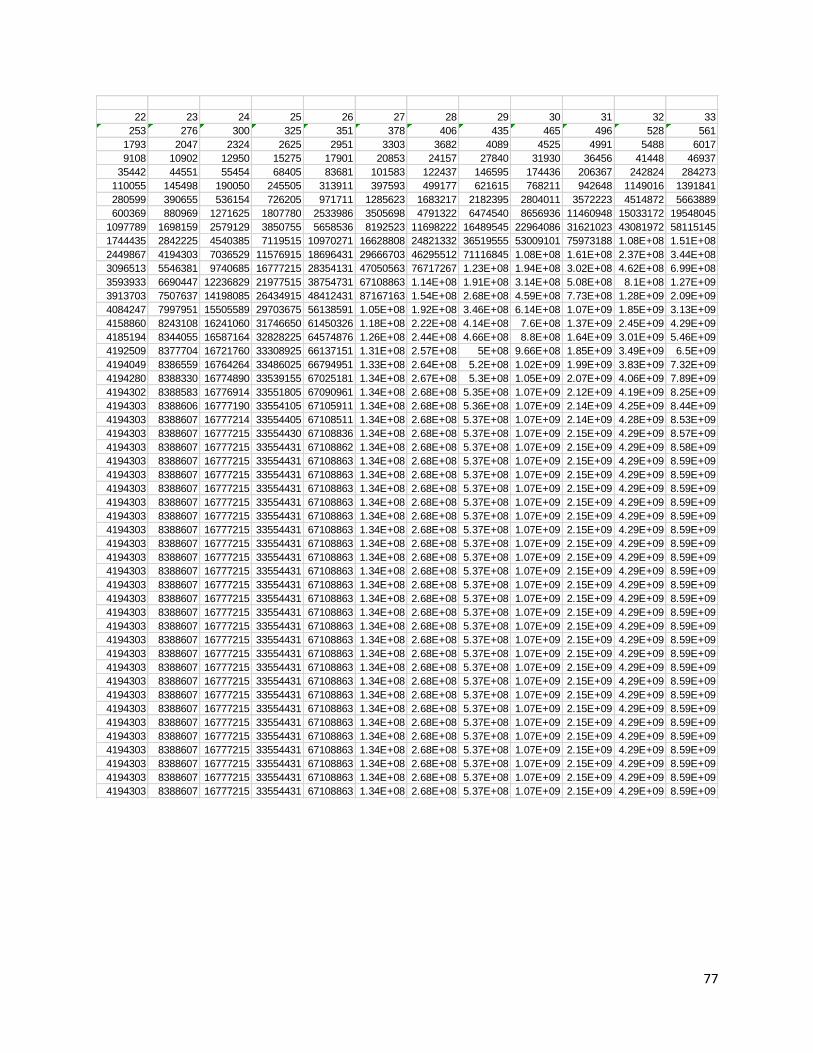
77

22 23 24 25 26 27 28 29 30 31 32 33

253 276 300 325 351 378 406 435 465 496 528 561

1793 2047 2324 2625 2951 3303 3682 4089 4525 4991 5488 6017

9108 10902 12950 15275 17901 20853 24157 27840 31930 36456 41448 46937

35442 44551 55454 68405 83681 101583 122437 146595 174436 206367 242824 284273

110055 145498 190050 245505 313911 397593 499177 621615 768211 942648 1149016 1391841

280599 390655 536154 726205 971711 1285623 1683217 2182395 2804011 3572223 4514872 5663889

600369 880969 1271625 1807780 2533986 3505698 4791322 6474540 8656936 11460948 15033172 19548045

1097789 1698159 2579129 3850755 5658536 8192523 11698222 16489545 22964086 31621023 43081972 58115145

1744435 2842225 4540385 7119515 10970271 16628808 24821332 36519555 53009101 75973188 1.08E+08 1.51E+08

2449867 4194303 7036529 11576915 18696431 29666703 46295512 71116845 1.08E+08 1.61E+08 2.37E+08 3.44E+08

3096513 5546381 9740685 16777215 28354131 47050563 76717267 1.23E+08 1.94E+08 3.02E+08 4.62E+08 6.99E+08

3593933 6690447 12236829 21977515 38754731 67108863 1.14E+08 1.91E+08 3.14E+08 5.08E+08 8.1E+08 1.27E+09

3913703 7507637 14198085 26434915 48412431 87167163 1.54E+08 2.68E+08 4.59E+08 7.73E+08 1.28E+09 2.09E+09

4084247 7997951 15505589 29703675 56138591 1.05E+08 1.92E+08 3.46E+08 6.14E+08 1.07E+09 1.85E+09 3.13E+09

4158860 8243108 16241060 31746650 61450326 1.18E+08 2.22E+08 4.14E+08 7.6E+08 1.37E+09 2.45E+09 4.29E+09

4185194 8344055 16587164 32828225 64574876 1.26E+08 2.44E+08 4.66E+08 8.8E+08 1.64E+09 3.01E+09 5.46E+09

4192509 8377704 16721760 33308925 66137151 1.31E+08 2.57E+08 5E+08 9.66E+08 1.85E+09 3.49E+09 6.5E+09

4194049 8386559 16764264 33486025 66794951 1.33E+08 2.64E+08 5.2E+08 1.02E+09 1.99E+09 3.83E+09 7.32E+09

4194280 8388330 16774890 33539155 67025181 1.34E+08 2.67E+08 5.3E+08 1.05E+09 2.07E+09 4.06E+09 7.89E+09

4194302 8388583 16776914 33551805 67090961 1.34E+08 2.68E+08 5.35E+08 1.07E+09 2.12E+09 4.19E+09 8.25E+09

4194303 8388606 16777190 33554105 67105911 1.34E+08 2.68E+08 5.36E+08 1.07E+09 2.14E+09 4.25E+09 8.44E+09

4194303 8388607 16777214 33554405 67108511 1.34E+08 2.68E+08 5.37E+08 1.07E+09 2.14E+09 4.28E+09 8.53E+09

4194303 8388607 16777215 33554430 67108836 1.34E+08 2.68E+08 5.37E+08 1.07E+09 2.15E+09 4.29E+09 8.57E+09

4194303 8388607 16777215 33554431 67108862 1.34E+08 2.68E+08 5.37E+08 1.07E+09 2.15E+09 4.29E+09 8.58E+09

4194303 8388607 16777215 33554431 67108863 1.34E+08 2.68E+08 5.37E+08 1.07E+09 2.15E+09 4.29E+09 8.59E+09

4194303 8388607 16777215 33554431 67108863 1.34E+08 2.68E+08 5.37E+08 1.07E+09 2.15E+09 4.29E+09 8.59E+09

4194303 8388607 16777215 33554431 67108863 1.34E+08 2.68E+08 5.37E+08 1.07E+09 2.15E+09 4.29E+09 8.59E+09

4194303 8388607 16777215 33554431 67108863 1.34E+08 2.68E+08 5.37E+08 1.07E+09 2.15E+09 4.29E+09 8.59E+09

4194303 8388607 16777215 33554431 67108863 1.34E+08 2.68E+08 5.37E+08 1.07E+09 2.15E+09 4.29E+09 8.59E+09

4194303 8388607 16777215 33554431 67108863 1.34E+08 2.68E+08 5.37E+08 1.07E+09 2.15E+09 4.29E+09 8.59E+09

4194303 8388607 16777215 33554431 67108863 1.34E+08 2.68E+08 5.37E+08 1.07E+09 2.15E+09 4.29E+09 8.59E+09

4194303 8388607 16777215 33554431 67108863 1.34E+08 2.68E+08 5.37E+08 1.07E+09 2.15E+09 4.29E+09 8.59E+09

4194303 8388607 16777215 33554431 67108863 1.34E+08 2.68E+08 5.37E+08 1.07E+09 2.15E+09 4.29E+09 8.59E+09

4194303 8388607 16777215 33554431 67108863 1.34E+08 2.68E+08 5.37E+08 1.07E+09 2.15E+09 4.29E+09 8.59E+09

4194303 8388607 16777215 33554431 67108863 1.34E+08 2.68E+08 5.37E+08 1.07E+09 2.15E+09 4.29E+09 8.59E+09

4194303 8388607 16777215 33554431 67108863 1.34E+08 2.68E+08 5.37E+08 1.07E+09 2.15E+09 4.29E+09 8.59E+09

4194303 8388607 16777215 33554431 67108863 1.34E+08 2.68E+08 5.37E+08 1.07E+09 2.15E+09 4.29E+09 8.59E+09

4194303 8388607 16777215 33554431 67108863 1.34E+08 2.68E+08 5.37E+08 1.07E+09 2.15E+09 4.29E+09 8.59E+09

4194303 8388607 16777215 33554431 67108863 1.34E+08 2.68E+08 5.37E+08 1.07E+09 2.15E+09 4.29E+09 8.59E+09

4194303 8388607 16777215 33554431 67108863 1.34E+08 2.68E+08 5.37E+08 1.07E+09 2.15E+09 4.29E+09 8.59E+09

4194303 8388607 16777215 33554431 67108863 1.34E+08 2.68E+08 5.37E+08 1.07E+09 2.15E+09 4.29E+09 8.59E+09

4194303 8388607 16777215 33554431 67108863 1.34E+08 2.68E+08 5.37E+08 1.07E+09 2.15E+09 4.29E+09 8.59E+09

4194303 8388607 16777215 33554431 67108863 1.34E+08 2.68E+08 5.37E+08 1.07E+09 2.15E+09 4.29E+09 8.59E+09

4194303 8388607 16777215 33554431 67108863 1.34E+08 2.68E+08 5.37E+08 1.07E+09 2.15E+09 4.29E+09 8.59E+09

4194303 8388607 16777215 33554431 67108863 1.34E+08 2.68E+08 5.37E+08 1.07E+09 2.15E+09 4.29E+09 8.59E+09

4194303 8388607 16777215 33554431 67108863 1.34E+08 2.68E+08 5.37E+08 1.07E+09 2.15E+09 4.29E+09 8.59E+09

4194303 8388607 16777215 33554431 67108863 1.34E+08 2.68E+08 5.37E+08 1.07E+09 2.15E+09 4.29E+09 8.59E+09

4194303 8388607 16777215 33554431 67108863 1.34E+08 2.68E+08 5.37E+08 1.07E+09 2.15E+09 4.29E+09 8.59E+09

4194303 8388607 16777215 33554431 67108863 1.34E+08 2.68E+08 5.37E+08 1.07E+09 2.15E+09 4.29E+09 8.59E+09

78

34 35 36 37 38 39 40 41 42 43 44

595 630 666 703 741 780 820 861 903 946 990

6579 7175 7806 8473 9177 9919 10700 11521 12383 13287 14234

52955 59535 66711 74518 82992 92170 102090 112791 124313 136697 149985

331211 384167 443703 510415 584934 667927 760098 862189 974981 1099295 1235993

1676115 2007327 2391495 2835199 3345615 3930550 4598478 5358577 6220767 7195749 8295045

7055731 8731847 10739175 13130671 15965871 19311487 23242038 27840517 33199095 39419863 46615613

25211935 32267667 40999515 51738691 64869363 80835235 1E+08 1.23E+08 1.51E+08 1.84E+08 2.24E+08

77663191 1.03E+08 1.35E+08 1.76E+08 2.28E+08 2.93E+08 3.74E+08 4.74E+08 5.97E+08 7.48E+08 9.33E+08

2.09E+08 2.86E+08 3.89E+08 5.24E+08 7.01E+08 9.28E+08 1.22E+09 1.59E+09 2.07E+09 2.67E+09 3.41E+09

4.95E+08 7.04E+08 9.9E+08 1.38E+09 1.9E+09 2.6E+09 3.53E+09 4.75E+09 6.35E+09 8.42E+09 1.11E+10

1.04E+09 1.54E+09 2.24E+09 3.23E+09 4.61E+09 6.52E+09 9.12E+09 1.27E+10 1.74E+10 2.38E+10 3.22E+10

1.97E+09 3.01E+09 4.55E+09 6.79E+09 1E+10 1.46E+10 2.12E+10 3.03E+10 4.29E+10 6.03E+10 8.41E+10

3.36E+09 5.33E+09 8.35E+09 1.29E+10 1.97E+10 2.97E+10 4.44E+10 6.55E+10 9.58E+10 1.39E+11 1.99E+11

5.22E+09 8.58E+09 1.39E+10 2.23E+10 3.52E+10 5.49E+10 8.46E+10 1.29E+11 1.94E+11 2.9E+11 4.29E+11

7.42E+09 1.26E+10 2.12E+10 3.51E+10 5.74E+10 9.26E+10 1.47E+11 2.32E+11 3.61E+11 5.55E+11 8.46E+11

9.76E+09 1.72E+10 2.98E+10 5.1E+10 8.62E+10 1.44E+11 2.36E+11 3.84E+11 6.16E+11 9.77E+11 1.53E+12

1.2E+10 2.17E+10 3.89E+10 6.87E+10 1.2E+11 2.06E+11 3.5E+11 5.86E+11 9.69E+11 1.58E+12 2.56E+12

1.38E+10 2.58E+10 4.75E+10 8.64E+10 1.55E+11 2.75E+11 4.81E+11 8.3E+11 1.42E+12 2.39E+12 3.97E+12

1.52E+10 2.9E+10 5.48E+10 1.02E+11 1.89E+11 3.44E+11 6.19E+11 1.1E+12 1.93E+12 3.35E+12 5.73E+12

1.61E+10 3.13E+10 6.04E+10 1.15E+11 2.17E+11 4.06E+11 7.5E+11 1.37E+12 2.47E+12 4.4E+12 7.74E+12

1.67E+10 3.28E+10 6.42E+10 1.25E+11 2.4E+11 4.57E+11 8.63E+11 1.61E+12 2.98E+12 5.45E+12 9.85E+12

1.7E+10 3.37E+10 6.65E+10 1.31E+11 2.55E+11 4.95E+11 9.52E+11 1.82E+12 3.43E+12 6.41E+12 1.19E+13

1.71E+10 3.41E+10 6.77E+10 1.34E+11 2.65E+11 5.2E+11 1.01E+12 1.97E+12 3.78E+12 7.21E+12 1.36E+13

1.72E+10 3.43E+10 6.83E+10 1.36E+11 2.7E+11 5.35E+11 1.06E+12 2.07E+12 4.04E+12 7.82E+12 1.5E+13

1.72E+10 3.43E+10 6.86E+10 1.37E+11 2.73E+11 5.43E+11 1.08E+12 2.13E+12 4.2E+12 8.24E+12 1.61E+13

1.72E+10 3.44E+10 6.87E+10 1.37E+11 2.74E+11 5.47E+11 1.09E+12 2.17E+12 4.3E+12 8.51E+12 1.67E+13

1.72E+10 3.44E+10 6.87E+10 1.37E+11 2.75E+11 5.49E+11 1.1E+12 2.19E+12 4.36E+12 8.66E+12 1.72E+13

1.72E+10 3.44E+10 6.87E+10 1.37E+11 2.75E+11 5.49E+11 1.1E+12 2.19E+12 4.38E+12 8.74E+12 1.74E+13

1.72E+10 3.44E+10 6.87E+10 1.37E+11 2.75E+11 5.5E+11 1.1E+12 2.2E+12 4.39E+12 8.77E+12 1.75E+13

1.72E+10 3.44E+10 6.87E+10 1.37E+11 2.75E+11 5.5E+11 1.1E+12 2.2E+12 4.4E+12 8.79E+12 1.76E+13

1.72E+10 3.44E+10 6.87E+10 1.37E+11 2.75E+11 5.5E+11 1.1E+12 2.2E+12 4.4E+12 8.79E+12 1.76E+13

1.72E+10 3.44E+10 6.87E+10 1.37E+11 2.75E+11 5.5E+11 1.1E+12 2.2E+12 4.4E+12 8.8E+12 1.76E+13

1.72E+10 3.44E+10 6.87E+10 1.37E+11 2.75E+11 5.5E+11 1.1E+12 2.2E+12 4.4E+12 8.8E+12 1.76E+13

1.72E+10 3.44E+10 6.87E+10 1.37E+11 2.75E+11 5.5E+11 1.1E+12 2.2E+12 4.4E+12 8.8E+12 1.76E+13

1.72E+10 3.44E+10 6.87E+10 1.37E+11 2.75E+11 5.5E+11 1.1E+12 2.2E+12 4.4E+12 8.8E+12 1.76E+13

1.72E+10 3.44E+10 6.87E+10 1.37E+11 2.75E+11 5.5E+11 1.1E+12 2.2E+12 4.4E+12 8.8E+12 1.76E+13

1.72E+10 3.44E+10 6.87E+10 1.37E+11 2.75E+11 5.5E+11 1.1E+12 2.2E+12 4.4E+12 8.8E+12 1.76E+13

1.72E+10 3.44E+10 6.87E+10 1.37E+11 2.75E+11 5.5E+11 1.1E+12 2.2E+12 4.4E+12 8.8E+12 1.76E+13

1.72E+10 3.44E+10 6.87E+10 1.37E+11 2.75E+11 5.5E+11 1.1E+12 2.2E+12 4.4E+12 8.8E+12 1.76E+13

1.72E+10 3.44E+10 6.87E+10 1.37E+11 2.75E+11 5.5E+11 1.1E+12 2.2E+12 4.4E+12 8.8E+12 1.76E+13

1.72E+10 3.44E+10 6.87E+10 1.37E+11 2.75E+11 5.5E+11 1.1E+12 2.2E+12 4.4E+12 8.8E+12 1.76E+13

1.72E+10 3.44E+10 6.87E+10 1.37E+11 2.75E+11 5.5E+11 1.1E+12 2.2E+12 4.4E+12 8.8E+12 1.76E+13

1.72E+10 3.44E+10 6.87E+10 1.37E+11 2.75E+11 5.5E+11 1.1E+12 2.2E+12 4.4E+12 8.8E+12 1.76E+13

1.72E+10 3.44E+10 6.87E+10 1.37E+11 2.75E+11 5.5E+11 1.1E+12 2.2E+12 4.4E+12 8.8E+12 1.76E+13

1.72E+10 3.44E+10 6.87E+10 1.37E+11 2.75E+11 5.5E+11 1.1E+12 2.2E+12 4.4E+12 8.8E+12 1.76E+13

1.72E+10 3.44E+10 6.87E+10 1.37E+11 2.75E+11 5.5E+11 1.1E+12 2.2E+12 4.4E+12 8.8E+12 1.76E+13

1.72E+10 3.44E+10 6.87E+10 1.37E+11 2.75E+11 5.5E+11 1.1E+12 2.2E+12 4.4E+12 8.8E+12 1.76E+13

1.72E+10 3.44E+10 6.87E+10 1.37E+11 2.75E+11 5.5E+11 1.1E+12 2.2E+12 4.4E+12 8.8E+12 1.76E+13

1.72E+10 3.44E+10 6.87E+10 1.37E+11 2.75E+11 5.5E+11 1.1E+12 2.2E+12 4.4E+12 8.8E+12 1.76E+13

79

45 46 47 48 49 50

1035 1081 1128 1176 1225 1275

15225 16261 17343 18472 19649 20875

164220 179446 195708 213052 231525 251175

1385979 1550200 1729647 1925356 2138409 2369935

9531039 10917019 12467220 14196868 16122225 18260635

54910659 64441699 75358719 87825940 1.02E+08 1.18E+08

2.7E+08 3.25E+08 3.9E+08 4.65E+08 5.53E+08 6.55E+08

1.16E+09 1.43E+09 1.75E+09 2.14E+09 2.61E+09 3.16E+09

4.35E+09 5.5E+09 6.93E+09 8.68E+09 1.08E+10 1.34E+10

1.45E+10 1.88E+10 2.43E+10 3.13E+10 4E+10 5.08E+10

4.33E+10 5.78E+10 7.66E+10 1.01E+11 1.32E+11 1.72E+11

1.16E+11 1.6E+11 2.17E+11 2.94E+11 3.95E+11 5.27E+11

2.83E+11 3.99E+11 5.59E+11 7.76E+11 1.07E+12 1.46E+12

6.28E+11 9.11E+11 1.31E+12 1.87E+12 2.65E+12 3.72E+12

1.27E+12 1.9E+12 2.81E+12 4.12E+12 5.99E+12 8.64E+12

2.38E+12 3.65E+12 5.55E+12 8.37E+12 1.25E+13 1.85E+13

4.09E+12 6.47E+12 1.01E+13 1.57E+13 2.4E+13 3.65E+13

6.53E+12 1.06E+13 1.71E+13 2.72E+13 4.29E+13 6.69E+13

9.7E+12 1.62E+13 2.69E+13 4.4E+13 7.12E+13 1.14E+14

1.35E+13 2.32E+13 3.94E+13 6.63E+13 1.1E+14 1.81E+14

1.76E+13 3.11E+13 5.42E+13 9.37E+13 1.6E+14 2.7E+14

2.17E+13 3.93E+13 7.04E+13 1.25E+14 2.18E+14 3.78E+14

2.55E+13 4.72E+13 8.65E+13 1.57E+14 2.81E+14 5E+14

2.87E+13 5.41E+13 1.01E+14 1.88E+14 3.45E+14 6.26E+14

3.11E+13 5.97E+13 1.14E+14 2.15E+14 4.03E+14 7.48E+14

3.28E+13 6.39E+13 1.24E+14 2.38E+14 4.53E+14 8.56E+14

3.39E+13 6.67E+13 1.31E+14 2.54E+14 4.92E+14 9.44E+14

3.46E+13 6.85E+13 1.35E+14 2.66E+14 5.2E+14 1.01E+15

3.49E+13 6.95E+13 1.38E+14 2.73E+14 5.39E+14 1.06E+15

3.51E+13 7E+13 1.39E+14 2.77E+14 5.5E+14 1.09E+15

3.51E+13 7.02E+13 1.4E+14 2.8E+14 5.57E+14 1.11E+15

3.52E+13 7.03E+13 1.41E+14 2.81E+14 5.6E+14 1.12E+15

3.52E+13 7.03E+13 1.41E+14 2.81E+14 5.62E+14 1.12E+15

3.52E+13 7.04E+13 1.41E+14 2.81E+14 5.63E+14 1.12E+15

3.52E+13 7.04E+13 1.41E+14 2.81E+14 5.63E+14 1.13E+15

3.52E+13 7.04E+13 1.41E+14 2.81E+14 5.63E+14 1.13E+15

3.52E+13 7.04E+13 1.41E+14 2.81E+14 5.63E+14 1.13E+15

3.52E+13 7.04E+13 1.41E+14 2.81E+14 5.63E+14 1.13E+15

3.52E+13 7.04E+13 1.41E+14 2.81E+14 5.63E+14 1.13E+15

3.52E+13 7.04E+13 1.41E+14 2.81E+14 5.63E+14 1.13E+15

3.52E+13 7.04E+13 1.41E+14 2.81E+14 5.63E+14 1.13E+15

3.52E+13 7.04E+13 1.41E+14 2.81E+14 5.63E+14 1.13E+15

3.52E+13 7.04E+13 1.41E+14 2.81E+14 5.63E+14 1.13E+15

3.52E+13 7.04E+13 1.41E+14 2.81E+14 5.63E+14 1.13E+15

3.52E+13 7.04E+13 1.41E+14 2.81E+14 5.63E+14 1.13E+15

3.52E+13 7.04E+13 1.41E+14 2.81E+14 5.63E+14 1.13E+15

3.52E+13 7.04E+13 1.41E+14 2.81E+14 5.63E+14 1.13E+15

3.52E+13 7.04E+13 1.41E+14 2.81E+14 5.63E+14 1.13E+15

3.52E+13 7.04E+13 1.41E+14 2.81E+14 5.63E+14 1.13E+15

80

9.4 LABVIEW VIRTUAL INSTRUMENT

design and development of an inexpensive acoustic ...my.fit.edu/~swood/john claus technical...

Documents