lecture notes on quicksortfp/courses/15122-s11/lectures/08-qsort.pdflecture notes on quicksort...

Lecture Notes onQuicksort

15-122: Principles of Imperative ComputationFrank Pfenning

Lecture 8February 3, 2011

1 Introduction

In this lecture we revisit the general description of quicksort from last lec-ture1 and develop an imperative implementation of it in C0. As usual, con-tracts and loop invariants will bridge the gap between the abstract idea ofthe algorithm and its implementation.

2 The Quicksort Algorithm

Quicksort again uses the technique of divide-and-conquer. We proceed asfollows:

1. Pick an arbitrary element of the array (the pivot).

2. Divide the array into two subarrays, those that are smaller and thosethat are greater (the partition phase).

3. Recursively sort the subarrays.

4. Put the pivot in the middle, between the two sorted subarrays to ob-tain the final sorted array.

In mergesort, it was easy to divide the input (we just picked the midpoint),but it was expensive to merge the results of the sorting the left and rightsubarrays. In quicksort, dividing the problem into subproblems could be

1omitted from the lecture notes there

LECTURE NOTES FEBRUARY 3, 2011

Quicksort L8.2

computationally expensive (as we analyze partitioning below), but puttingthe results back together is immediate. This kind of trade-off is frequent inalgorithm design.

Let us analyze the asymptotic complexity of the partitioning phase ofthe algorithm. Say we have the array

{3, 1, 4, 4, 7, 2, 8}

and we pick 3 as our pivot. Then we have to compare each element of this(unsorted!) array to the pivot to obtain a partition such as

lt = {2, 1}, pivot = 3, geq = {4, 7, 8, 4}

We have picked an arbitrary order for the elements in the subarrays; all thatmatters is that all smaller ones are to the left of the pivot and all larger onesare to the right.

Since we have to compare each element to the pivot, but otherwisejust collect the elements, it seems that the partition phase of the algorithmshould have complexity O(k), where k is the length of the array segmentwe have to partition.

How many recursive calls do we have in the worst case, and how longare the subarrays? In the worst case, we always pick either the smallest orlargest element in the array so that one side of the partition will be empty,and the other has all elements except for the pivot itself. In the exampleabove, the recursive calls might proceed as follows:

call pivotqsort({3, 1, 4, 4, 7, 2, 8}) 1qsort({3, 4, 4, 7, 2, 8}) 2qsort({3, 4, 4, 7, 8}) 3qsort({4, 4, 7, 8}) 4qsort({4, 7, 8}) 4qsort({7, 8}) 7qsort({8})

All other recursive calls are with the empty array segment, since we neverhave any elements less than the pivot. We see that in the worst case thereare n − 1 significant recursive calls for an array of size n. The kth recur-sive call has to sort a subarray of size k, which proceeds by partitioning,requiring O(k) comparisons.


Quicksort L8.3

This means that, overall, for some constant c we have

c

n−1∑i=0

i = cn(n− 1)

2∈ O(n2)

comparisons. Here we used the fact that O(p(n)) for a polynomial p(n) isalways equal to the O(nk) where k is the leading exponent of the polyno-mial. This is because the largest exponent of a polynomial will eventuallydominate the function, and big-O notation ignores constant coefficients.

So quicksort has quadratic complexity in the worst case. How can wemitigate this? If we always picked the median among the elements in thesubarray we are trying to sort, then half the elements would be less andhalf the elements would be greater. So in this case there would be onlylog(n) recursive calls, where at each layer we have to do a total amount ofn comparisons, yielding an asymptotic complexity of O(n ∗ log(n)).

Unfortunately, it is not so easy to compute the median to obtain theoptimal partitioning. It turns out that if we pick a random element, it willbe on average close enough to the median that the expected running timeof algorithm is still O(n ∗ log(n)).

We really should make this selection randomly. With a fixed-pick strat-egy, there may be simple inputs on which the algorithm takes O(n2) steps.For example, if we always pick the first element, then if we supply an arraythat is already sorted, quicksort will take O(n2) steps (and similarly if itis “almost” sorted with a few exceptions)! If we pick the pivot randomlyeach time, the kind of array we get does not matter: the expected runningtime is always the same, namely O(n ∗ log(n)). This is an important use ofrandomness to obtain a reliable average case behavior.

3 The qsort Function

We now turn our attention to developing an imperative implementation ofquicksort, following our high-level description. We implement quicksortin the function qsort as an in-place sorting function that modifies a givenarray instead of creating a new one. It therefore returns no value, which isexpressed by giving a return type of void.

void qsort(int[] A, int lower, int upper)//@requires 0 <= lower && lower <= upper && upper <= \length(A);//@ensures is_sorted(A, lower, upper);{


Quicksort L8.4

...}

We sort the segment A[lower ..upper) of the array between lower (inclu-sively) and upper (exclusively). The precondition in the @requires an-notation verifies that the bounds are meaningful with respect to A. Thepostcondition in the @ensures clause guarantees that the given segment issorted when the function returns. It does not express that the output isa permutation of the input, which is required to hold but is not formallyexpressed in the contract (see Exercise 1).

Before we start the body of the function, we should consider how toterminate the recursion. We don’t have to do anything if we have an arraysegment with 0 or 1 elements. So we just return if upper − lower ≤ 1.

void qsort(int[] A, int lower, int upper)//@requires 0 <= lower && lower <= upper && upper <= \length(A);//@ensures is_sorted(A, lower, upper);{if (upper-lower <= 1) return;...

}

Next we have to call a partition function. We want partitioning to bedone in place, modifying the array A. Still, partitioning needs to returnthe index i of the pivot element because we then have to recursively sortthe two subsegments to the left and right of the where the pivot is afterpartitioning. So we declare:

int partition(int[] A, int lower, int upper)//@requires 0 <= lower && lower < upper && upper <= \length(A);//@ensures lower <= \result && \result < upper;//@ensures gt(A[\result], A, lower, \result);//@ensures leq(A[\result], A, \result+1, upper);;

Here we use the auxiliary functions gt (for greater than) and leq (for less orequal), where

• gt(x, A, lower, i) if x > y for every y in A[lower ..i).

• leq(x, A, i+1, upper) if x ≤ y for very y in A[i + 1..upper).


Quicksort L8.5

Their definitions can be found in the qsort.c0 file on the course web pages.Some details on this specification: we require lower < upper because if

they were equal, then the segment could be empty and we cannot possiblypick a pivot element or return its index. We ensure that result < upper sothat the index of the pivot is a legal index in the segment A[lower ..upper).

Now we can fill in the remainder of the main sorting function.

void qsort(int[] A, int lower, int upper)//@requires 0 <= lower && lower <= upper && upper <= \length(A);//@ensures is_sorted(A, lower, upper);{if (upper-lower <= 1) return;int i = partition(A, lower, upper);qsort(A, lower, i);qsort(A, i+1, upper);return;

}

It is a simple but instructive exercise to reason about this program, usingonly the contract for partition together with the preconditions for qsort(see Exercise 2).

To show that the qsort function terminates, we have to show the arraysegment becomes strictly smaller in each recursive call. First, i − lower <upper − lower since i < upper by the postcondition for partition. Sec-ond, upper − (i + 1) < upper − lower because i + 1 > lower , also by thepostcondition for partition.

4 Partitioning

The trickiest aspect of quicksort is the partitioning step, in particular sincewe want to perform this operation in place. Once we have determinedthe pivot element, we want to divide the array segment into four different


http://www.cs.cmu.edu/~fp/courses/15122-s11/lectures/08-qsort/qsort.c0

Quicksort L8.6

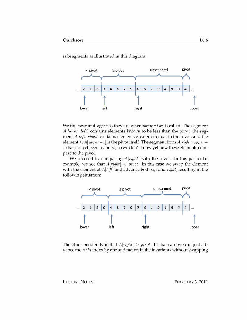
subsegments as illustrated in this diagram.

2 1 3 7 4 8 7 9 0 6 1 9 4 8 3 4

<pivot ≥pivot unscanned pivot

lower le3 right upper

… …

We fix lower and upper as they are when partition is called. The segmentA[lower ..left) contains elements known to be less than the pivot, the seg-ment A[left ..right) contains elements greater or equal to the pivot, and theelement at A[upper−1] is the pivot itself. The segment from A[right ..upper−1) has not yet been scanned, so we don’t know yet how these elements com-pare to the pivot.

We proceed by comparing A[right ] with the pivot. In this particularexample, we see that A[right ] < pivot . In this case we swap the elementwith the element at A[left ] and advance both left and right , resulting in thefollowing situation:

2 1 3 0 4 8 7 9 7 6 1 9 4 8 3 4



… …

The other possibility is that A[right ] ≥ pivot . In that case we can just ad-vance the right index by one and maintain the invariants without swapping


Quicksort L8.7

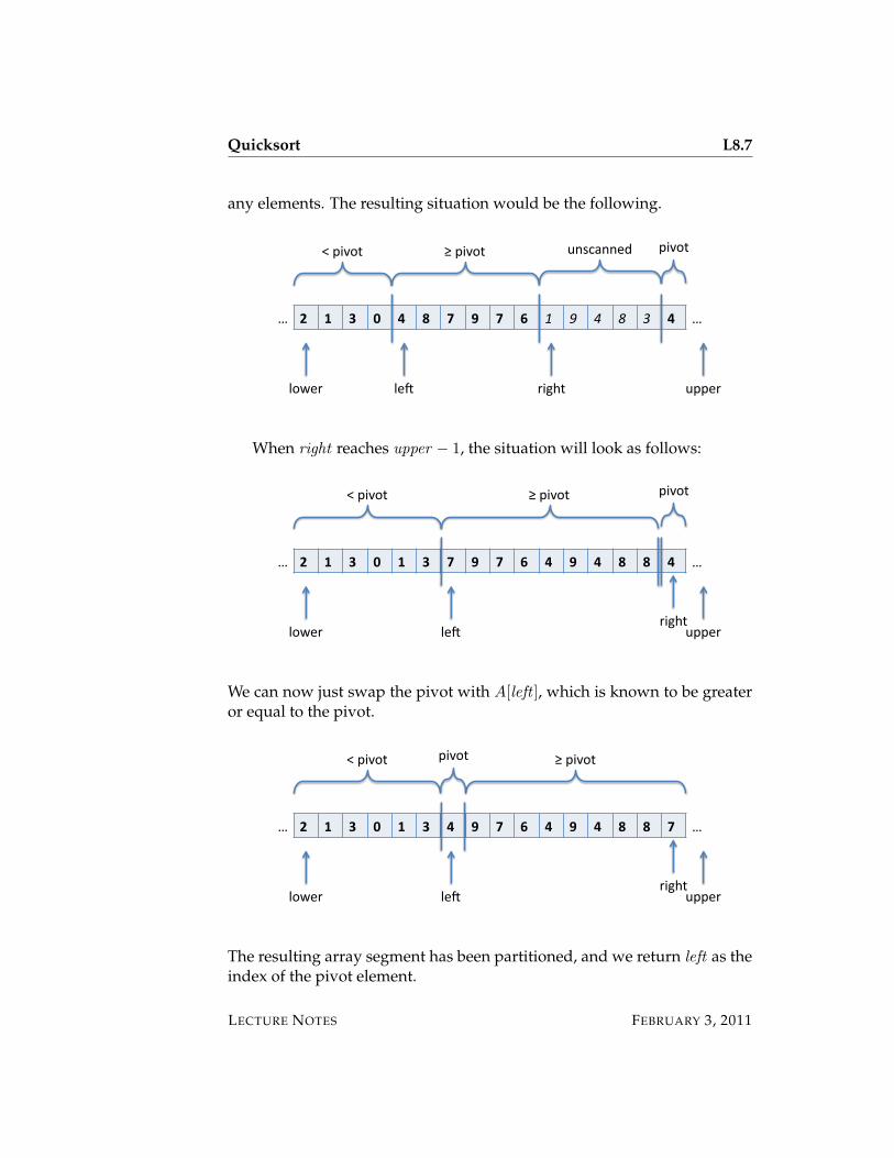
any elements. The resulting situation would be the following.

2 1 3 0 4 8 7 9 7 6 1 9 4 8 3 4



… …

When right reaches upper − 1, the situation will look as follows:

2 1 3 0 1 3 7 9 7 6 4 9 4 8 8 4

<pivot ≥pivot pivot

lower le-right

upper

… …

We can now just swap the pivot with A[left ], which is known to be greateror equal to the pivot.

2 1 3 0 1 3 4 9 7 6 4 9 4 8 8 7

<pivot ≥pivotpivot

lower le-right

upper

… …

The resulting array segment has been partitioned, and we return left as theindex of the pivot element.


Quicksort L8.8

Throughout this process, we have only ever swapped two elements ofthe array. This guarantees that the array segment after partitioning is apermutation of the segment before.

However, we did not consider how to start this algorithm. We begin bypicking a random element as the pivot and then swapping it with the lastelement in the segment. We then initialize left and right to lower . We thenhave the situation

2 4 1 7 3 8 7 9 0 6 1 9 4 8 3 4

unscanned pivot

lowerle1

right upper

… …

where the two segments with smaller and greater elements than the pivotare still empty.

In this case (where left = right), if A[right ] ≥ pivot then we can incre-ment right as before, preserving the invariants for the segments. However,if A[left ] < pivot , swapping A[left ] with A[right ] has no effect. Fortunately,incrementing both left and right preserves the invariant since the elementwe just checked is indeed less than the pivot.

2 4 1 7 3 8 7 9 0 6 1 9 4 8 3 4

unscanned pivot

lowerle1

right upper

… …

If left and right ever separate, we are back to the generic situation we dis-


Quicksort L8.9

cussed at the beginning. In this example, this happens in the next step.

2 4 1 7 3 8 7 9 0 6 1 9 4 8 3 4

unscanned pivot

lowerle1

right upper

… …

<pivot ≥pivot

If left and right always stay the same, all elements in the array segment arestrictly less than the pivot, excepting only the pivot itself. In that case, too,swapping A[left ] and A[right ] has no effect and we return left = upper − 1as the correct index for the pivot after partitioning.

Implementing Partitioning

Now that we understand the algorithm and its correctness proof, it remainsto turn these insights into code. We start by computing the index of thepivot and move the pivot to A[upper − 1]. To keep the code simple, we takethe midpoint of the segment instead of randomly selecting one. This willwork well if the array is random, or if it is almost sorted.

int partition(int[] A, int lower, int upper)//@requires 0 <= lower && lower < upper && upper <= \length(A);//@ensures lower <= \result && \result < upper;//@ensures gt(A[\result], A, lower, \result);//@ensures leq(A[\result], A, \result+1, upper);{int pivot_index = lower+(upper-lower)/2;int pivot = A[pivot_index];swap(A, pivot_index, upper-1);...

}

At this point we initialize left and right to lower . We scan the array usingthe index right until it reaches upper − 1.


Quicksort L8.10

int pivot_index = lower+(upper-lower)/2;int pivot = A[pivot_index];swap(A, pivot_index, upper-1);int left = lower;int right = lower;while (right < upper-1)...{}

Next, we should turn the observations about the state of the algorithmmade in the preceding section into loop invariants. The zeroth one justrecords the relative position of the indices into the array. The first onestates that the pivot is strictly greater than any element in the segmentA[lower ..left). The second states the the pivot is less or equal any element inthe segment A[left ..right). The third one expresses that the pivot is storedat A[upper − 1]

swap(A, pivot_index, upper-1);int left = lower;int right = lower;while (right < upper-1)//@loop_invariant lower <= left && left <= right && right < upper;//@loop_invariant gt(pivot, A, lower, left);//@loop_invariant leq(pivot, A, left, right);//@loop_invariant pivot == A[upper-1];{...

}

It is easy to verify that the invariants are satisfied initially, given that wealso know lower < upper from the function precondition.


Quicksort L8.11

In the body of the loop we compare the pivot with A[right ] and, in eachcase, take the appropriate actions described in the previous section.

while (right < upper-1)//@loop_invariant lower <= left && left <= right && right < upper;//@loop_invariant gt(pivot, A, lower, left);//@loop_invariant leq(pivot, A, left, right);//@loop_invariant pivot == A[upper-1];{if (pivot <= A[right]) {right++;

} else {swap(A, left, right);left++;right++;

}}

Again, it is straightforward to check that the loop invariant is preserved,based on the description in the previous section. It is important to distin-guish the special case that left = right when the second invariant (leq(...))is vacuously satisfied.

At the end, we swap A[left ] with A[upper − 1] and return left as theindex of the pivot in the partitioned arrays. The complete code is on thenext page


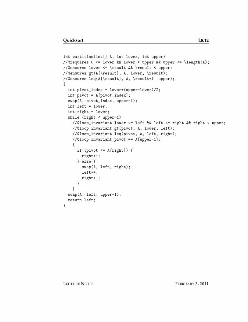
Quicksort L8.12

int partition(int[] A, int lower, int upper)//@requires 0 <= lower && lower < upper && upper <= \length(A);//@ensures lower <= \result && \result < upper;//@ensures gt(A[\result], A, lower, \result);//@ensures leq(A[\result], A, \result+1, upper);{int pivot_index = lower+(upper-lower)/2;int pivot = A[pivot_index];swap(A, pivot_index, upper-1);int left = lower;int right = lower;while (right < upper-1)//@loop_invariant lower <= left && left <= right && right < upper;//@loop_invariant gt(pivot, A, lower, left);//@loop_invariant leq(pivot, A, left, right);//@loop_invariant pivot == A[upper-1];{if (pivot <= A[right]) {right++;

} else {swap(A, left, right);left++;right++;

}}

swap(A, left, upper-1);return left;

}


Quicksort L8.13

Exercises

Exercise 1 In this exercise we explore strengthening the contracts on in-placesorting functions.

1. Write a function is_permutation which checks that one segment of anarray is a permutation of another.

2. Extend the specifications of sorting and partitioning to include the permu-tation property.

3. Discuss any specific difficulties or problems that arise. Assess the outcome.

Exercise 2 Prove that the precondition for qsort together with the contract forpartition implies the postcondition. During this reasoning you may also assumethat the contract holds for recursive calls.

Exercise 3 Our implementation of partitioning did not pick a random pivot, buttook the middle element. Construct an array with seven elements on which ouralgorithm will exhibit its worst-case behavior, that is, on each step, one of the par-titions is empty.


lecture notes on quicksortfp/courses/15122-s11/lectures/08-qsort.pdflecture notes on quicksort...

Documents