pdfs.semanticscholar.org. di cosmo and d. kesner 2 n, give the same result m n. similarly for pairs,...
TRANSCRIPT

Math. Struct. in Comp. Science (1993), vol. 11, pp. 1–000 Copyright c Cambridge University Press
Simulating expansions without expansions
Roberto Di CosmoyDelia Kesner {Received
We add extensional equalities for the functional and product types to the typed �-calculus with not only productsand terminal object, but also sums and bounded recursion (a version of recursion that does not allow recursive callsof infinite length). We provide a confluent and strongly normalizing (thus decidable) rewriting system for thecalculus, that stays confluent when allowing unbounded recursion. For that, we turn the extensional equalities intoexpansion rules, and not into contractions as is done traditionally. We first prove the calculus to be weaklyconfluent, which is a more complex and interesting task than for the usual �-calculus. Then we provide an effectivemechanism to simulate expansions without expansion rules, so that the strong normalization of the calculus can bederived from that of the underlying, traditional, non extensional system. These results give us the confluence of thefull calculus, but we also show how to deduce confluence directly form our simulation technique, without the weakconfluence property.
1. Introduction
Over the past years there has been a growing interest in the properties of �-calculus extended with variousdifferent type constructors, in particular pairs and sums, used to represent common data types. For these typeconstructors it is customary to provide a set of equalities that are then turned into computation rules: this is thecase, for example, of the elimination rules for pairs:(�1) �1(hM;Ni) = M (�2) �2(hM;Ni) = N
They tell us how to operationally compute with objects of these types: if we have a pair hM;Ni, then wecan decompose it to access its first or second component.
There is anyway something else that one likes to do with �-calculus, besides using �-terms as programs tobe computed: one would like to reason about programs, to prove that they enjoy certain properties. Here iswhere extensional equalities come into play. In the case of functions, for example, since the only operationalway to use a function is to apply it to an argument, we do not really want to consider a term M of function typedifferent from the term �x:Mx where x does not occur free in M : both terms, when applied to an argumenty DMI-LIENS (CNRS URA 1347) Ecole Normale Superieure - 45, Rue d’Ulm - 75230 Paris France
E-mail:[email protected]{ INRIA Rocquencourt - Domaine de Voluceau, BP 105 - 78153 Le Chesnay Cedex, France andCNRS and LRI - Bat 490, Universite de Paris-Sud - 91405 Orsay Cedex, FranceE-mail:[email protected]

R. Di Cosmo and D. Kesner 2N , give the same result MN . Similarly for pairs, the only operational way to use a pair is by projecting out thefirst or the second component, so we do not want to consider a term M of product type different from the termh�1(M); �2(M)i: the result of accessing any of these two terms via a first or second projection is the sameterm �1(M) or �2(M).
These facts can be incorporated in the calculus in the form of equalities, that one can read in at least twodifferent ways:
— an operational way: these equalities just state possible optimizations of a program. Since a term h�1(M); �2(M)iis more complex then M , but behaves the same way, it is convenient to replace all its occurrences by M ,as this transformation will yield an equivalent, but more efficient and smaller program. Similarly, we willreplace every occurrence of �x:Mx by M .
— a theoretical way: these equalities state a relation between a program and its type. They just tell us thatwhenever a term M has a functional type, then it must really be a function, built by �-abstraction, so weought to replace it by �x:Mx if it is not already a function. Similarly, a term M of product type has to bereally a pair, built via the pair constructor, or otherwise it must be replaced by h�1(M); �2(M)i.
As we will briefly see in the Survey, a lot of research activity has focused on the operational reading of theseequalities in the tradition of �-calculus, while only a little on the theoretical one. In this paper we will showhow this last reading of the equalities provides a confluent and strongly normalizing reduction system for thesimply typed �-calculus with pairs, sums, unit type (or terminal object) and a bounded recursion operator. Wealso show that the same reduction system stays confluent when allowing unbounded recursion, while of courseloosing the strong normalization property.
1.1. Survey
Due to the deep connections between �-calculus, proof theory and category theory, works on extensionalequalities have appeared with different motivations in all these fields.
By far, the best known extensional equality is the � axiom that we informally introduced above, written inthe �-calculus formalism as(�) �x:Mx =M provided x is not free in MThis axiom, also known as extensionality, has traditionally been turned into a reduction, carrying the samename, by orienting the equality from left to right, interpreting operationally equality as a contraction. Such aninterpretation is well behaved as it preserves confluence (CF58).
In the early 70’s, the attention was focusing on products and the extensional rule for pairs, called surjectivepairing, which is the analog for product types of the usual � extensional rule.(SP ) h�1(M); �2(M)i = MWith the previous experience of the � rule, it is easy to understand how, at that time, most of the people thoughtthat the right way to turn such an equality into a rewrite rule was also from left to right, as a contraction. But in1980, J.W. Klop discovered (Klo80) that, if added to the usual confluent rewrite rules for pure �-calculus, thisinterpretation of SP breaks confluencey.
Anyway, this first negative result was shortly after mitigated in (Pot81) for the simply typed �-calculus withy See (Bar84), p. 403-409 for a short history and references.

Simulating expansions without expansions 3� and SP contractions, by providing a first proof of confluence and strong normalization, later on simplifiedin different ways (see (Tro86) or (GLT90), for example). From then on, the contraction rule for SP was notconsidered harmful in a typed framework, until the seminal work by Lambek and Scott (LS86). There, thedecision problem of the equational theory of Cartesian Closed Categories (ccc’s) is solved using a particulartyped �-calculus equipped with not only � and SP equalities, but also with a special type T representing theterminal object of the ccc’sz. This distinguished atomic type comes with a further extensional axiom assertingthat there is exactly one term � of type T: (Top) M : T = �Now, the type T has the bad property of destroying confluence, if the extensional equalities � and SP areturned into contraction rules: the following are the critical pairs that arise immediately, as first pointed out byObtulowicz, (see (LS86)): h�1(x); �2(x)i )SP x h�1(x); �2(x)i )SP x+Top +Toph�; �2(x)i h�1(x); �i(�x : T:Mx) : T! A)� M (�x : A:Mx) : A! T)� M+Top +Top(�x : T:M�) : T! A (�x : A:�) : A! T
It is indeed possible, but not easy, to extend the contractive reduction system in order to recover confluence.A first step towards such a confluent system was taken by Poigne and Voss, who were not inspired by categorytheory, but by the implementation of algebraic data types (PV87). In their paper, they study a calculus thatincludes �1����, and notice that to solve the previous critical pairs one needs to add an infinite numberof reduction rules (that can be anyway finitely described). Then confluence of such an extended systemcan be proved by showing weak confluence and strong normalization. Unfortunately, the critical pair for(�x : A:Mx) : T! A is missing there, and the strong normalization proof is incomplete.
More recently, Curien and the first author got interested in a polymorphic extension of �1����, that arosein the study of the theory of object oriented programming and of isomorphisms of types (CDC91). They give acomplete (infinite) set of reduction rules for the calculus, which is proved confluent using just weak confluence,weak normalization and some additional properties.
Meanwhile, in the field of proof theory, Prawitz was suggesting (Pra71) to turn these extensional equalitiesinto expansion rules, rather than contractions. Building on such ideas, but motivated by the study of coherenceproblems in category theory, Mints gives a first faulty proof that in the typed framework expansion rules, ifhandled with care, are weakly normalizing and preserve confluence of the typed calculus (Min79)x.
This idea of using expansion rules seems to have passed unnoticed for a long time, even if the so called �-longnormal forms were well known and used in the study of higher order unification problems (Hue76): only inz This is the Unit type in languages like ML.x The same idea is present in (Min77).

R. Di Cosmo and D. Kesner 4
these last years there has been a renewed interest in expansion rules. In recent work (Jay92), still motivated bycategory theoretic investigation, Jay explores a simply typed �-calculus with just T and a natural number typeN as base types, equipped with an induction combinator for terms of type N. He introduced expansion rules for� and SP that are exactly the same as the ones originally used by Mints, and in (JG92) this calculus is provedconfluent and strongly normalizing. Category theory is also the motivation of Cubric (Cub92), who repairedthe error in the original proof by Mints, showing confluence (by means of a careful study of residuals) and alsoweak normalization (but not strong normalization). An interesting divide-and-conquer approach is proposedin (Aka93), where confluence and strong normalization are shown in a modular way. Finally, in (Dou93),confluence is shown via the usual Newman’s Lemma and strong normalization by means of a variation of thereducibility proof based on introduction rather than elimination terms.
1.2. Our work
The present paper is inspired especially by (Jay92) and (PV87). We use expansion rules to provide a confluentrewriting system for the typed �-calculus with not only products and terminal object, but also sums andrecursion. This result is derived from the confluence of a restricted system where recursion is bounded (recursivecalls of infinite length are not allowed), which is proved to be weakly confluent and strongly normalizing.
We show that strong normalization of the full system can be reduced to that of the system without expansionrules, for which the traditional techniques can be used. For that purpose, we show that any one step reductionin the calculus with expansions can be simulated by a non-empty reduction sequence in the calculus withoutexpansions. It turns out that this result is powerful enough to prove directly also the confluence property, asshown in section 7.
Since the reduction with expansion rules is not a congruence, several fundamental properties that hold forthe well known typed �-calculi have to be reformulated in the expansionary framework in a different way aswe will see in Section 4. For this reason we believe that the system with expansion rules deserves to be studiedmuch more carefully, so we will undertake the task of proving directly weak confluence: this will lead us touncover many of the essential features of this reduction.
We introduce now the calculus and its reduction system in section 2, then we investigate the key propertiesof the new reduction system: weak confluence (section 4) and strong normalization (section 5). In section 7we derive the confluence property in two different ways and finally in the conclusion we discuss some furtherapplications of our proof techniques.
An extended abstract of this work can be found in (DCK93a).
2. The Calculus
It is now time to introduce the calculus we will deal with in this paper. There are two versions, one with boundedrecursion, and the other with unbounded recursion, that differ just in the term formation rule and in the equalityrule for recursive terms. We will now introduce the calculus with bounded recursion and then describe how theunbounded version can be obtained from it.

Simulating expansions without expansions 5
2.1. Types and Terms
The set of types of our calculus contains a distinguished type constant T{, a denumerable set of atomic or basetypes, and is closed w.r.t. formation of function, product and sum, i.e. if A and B are types, then also A! B,A�B and A+B are types.
For each type A, we fix a denumerable set of variables of that type. We will use x; y; z; : : : to range overvariables, and for a term M we write M : A to mean that M is a term of type A.
The term formation rules of the calculus can then be presented as follows.
Γ ` � : T1 � i � n and the xi’s are pairwise distinctx1 : A1; : : : ; xn : An ` xi : Ai
Γ; x : A `M : BΓ ` �x : A:M : A! B Γ `M : A! B Γ ` N : A
Γ ` (MN) : BΓ `M : A Γ ` N : B
Γ ` hM;Ni : A�B Γ `M : B1 �B2 i = 1; 2Γ ` �i(M) : Bi
Γ `M : Bi i = 1; 2Γ ` iniB1+B2
(M) : B1 +B2
Γ ` P : A1 +A2 Γ `Mi : Ai ! DΓ ` Case(P;M1;M2) : D
Γ; x : A `M : A i � 0Γ ` (rec x : A:M)i : A
We may omit types of variables in �-abstractions when they are clear from the context writing �y:M insteadof �y : C:M .
Notation 2.1. (Free variables, substitutions)The set of free variables of a term M will be noted FV (M). It can be defined inductively as follows:
{ This stands for the terminal object in ccc’s or for the Unit type in languages like ML.

R. Di Cosmo and D. Kesner 6FV (�) =;FV (x) =fxgFV (OA) =FV (M)FV (MN) =FV (M) + FV (N)FV (hM;Ni) =FV (M) + FV (N)FV (�x : A:M) =FV (M)� fxgFV ((rec x : A:M)i) =FV (M)� fxgFV (in1C(M)) =FV (M)FV (in2C(M)) =FV (M)FV (�1(M)) =FV (M)FV (�2(M)) =FV (M)FV (Case(P;M;N))=FV (P ) + FV (M) + FV (N)We write [N1; : : : ; Nn=x1; : : : ; xn] (often abbreviated [N=x]) for the typed substitution mapping each variablexi : Ai to a term Ni : Ai. We write M [N=x] for the term M where each variable xi free in M is replaced byNi.2.2. Equality
Besides the usual identification of terms up to � conversion (i.e. renaming of bound variables), our calculus isequipped with the equality E on terms generated from the following axioms.(�) (�x : A:M)N = M [N=x](�1) �1(hM1;M2i) = M1(�2) �2(hM1;M2i) = M2(�) Case(in1C(R);M1;M2) = M1RCase(in2C(R);M1;M2) = M2R(rec) (rec y : C:M)i+1 = M [(rec y : C:M)i=y](�) �x : A:Mx = M if
� x 62 FV (M)M : A! B(�) h�1(M); �2(M)i = M if M : A�B(Top) M = � if M : TThe index i that is attached to each rec term is a bound on the depth of the recursive calls that can originate
from it. With such a bound, it is possible to insure the strong normalization of the associated reduction system.The unbounded system is obtained from the bounded one by simply erasing all the bound indexes from the
formation and equality rules (and the associated reduction rules). As we will show later, the bounded system cansimulate any finite reduction of the unbounded system, and this fact will make it easy to extend the confluenceresult for the bounded system to the unbounded one. For simplicity, we will explicitly note the bound indexonly when necessary, dropping it whenever the properties we discuss hold in both systems.
3. The confluent rewriting system
The non extensional equality rules and the rule for T can be turned into a confluent rewriting system by orientingthem from left to right, as follows

Simulating expansions without expansions 7(�) (�x : A:M)N �! M [N=x](�i) �i(hM1;M2i) �! Mi; for i = 1; 2(�) Case(iniC(R);M1;M2) �! MiR; for i = 1; 2(rec) (rec y : C:M)i+1 �! M [(rec y : C:M)i=y]; for i � 0(Top) M �! � if M : T and M 6= �But when we want to turn the extensional equalities for functions and pairs into expansions, as explained
very clearly by Jay (Jay92), we must be careful to avoid the following reduction loops:�x:M ; �y:(�x:M)y ; �y:M [y=x] =� �x:MhM;Ni ; h�1(hM;Ni); �2(hM;Ni)i ; hM;NiMN ; (�x:Mx)N ; MN�i(P ) ; �i(h�1(P ); �2(P )i) ; �i(P )To break the first two loops we must disallow expansions of terms that are already �-abstractions or pairs:(�) M �! �x : A:Mx if
� x 62 FV (M)M : A! B and M is not a �-abstraction(�) M �! h�1(M); �2(M)i if� M : A�B and M is not a pair
But this is not enough: to break the last two loops we must also forbid the � expansion of a term in a contextwhere this term is applied to an argument, and � expansion of a term when such a term is the argument ofa projection. This means that we cannot define the one-step reduction relation =) on terms as the leastcongruence on terms containing the above reductions �! , as is done usually. Instead, one defines formallyM =)M 0 starting from �! by induction on the structure of the term. The definition is the same as acongruence closure but for the two last cases.
We will write M 1;:::; n�! M 0 if M i�!M 0, for some i and: �! stands for a �! step that is not a step.
The one-step reduction relation between terms, denoted =) is defined as follows:
Definition 3.1. (One-step reduction)� If M �!M 0, then M =)M 0� If M =)M 0, then (rec x : A:M)i =) (rec x : A:M 0)iCase(M;N;O) =) Case(M 0; N;O) in1C(M) =) in1C(M 0) hM;Ni =) hM 0; NiCase(N;M;O) =) Case(N;M;0O) in2C(M) =) in2C(M 0) hN;Mi =) hN;M 0iCase(N;O;M) =) Case(N;O;M 0) � x : A:M =) � x : A:M 0 NM =) NM 0� If M =)M 0 but M :��!M 0, then MN =)M 0N� If M =)M 0 but M :��!M 0, then �i(M) =) �i(M 0) for i = 1; 2Notation 3.2. The transitive and the reflexive transitive closure of =) are noted=)+ and =)� respectively.Similarly we define
1=) ,1=)+ and
1=)� for the unbounded system.
We will use some standard notions from the theory of rewriting system, such as redex, normal form,confluence, weak confluence, strong normalization, etc, without explicitly redefining them here.
It is also useful to define a notion of influential positions of a term: informally, a position in a term isinfluential if the subterm occurring at that position cannot be expanded at the root. For example, M occurs atan influential position in the term MN , as � expansion is forbidden on M , no matters if it is a �-abstractionor not. Obviously, a position in a term can be influential for � or for �, but not for both. This notion can beproperly formalized by induction on the structure of the terms (see (DCK93b)).

R. Di Cosmo and D. Kesner 8
3.1. Adequacy of expansions for extensional equalities
First of all, it is necessary to show that the limitations imposed on the reduction system do not make us looseany valid equality. We will show that the reduction system just introduced really generates the equalities wedefined for the calculus. This comes from the fact that the limitations imposed on the reductions are introducedexactly to avoid reduction loops.
Theorem 3.3. ( =) generates E) The equality E and the reflexive, symmetric and transitive closure R of=) are the same relation.
Proof. The fact that R is included in E is evident, as all the reductions rules are derived from the equalityaxioms by orienting and restricting them.What we are left to show is E � R. It is enough to show that whenever M = N comes from a single equalityaxiom, we can either rewrite M to N or N to M (sinceR is reflexive, symmetric and transitive, the other caseswill follow trivially).The basic idea of the proof is to associate to each of these equality steps a reduction step in R. This is done inthe obvious way, except in the cases that would violate one of the restrictions imposed on the expansion rules,which we will solve using exactly the reduction loop that this restriction is supposed to prevent.Here are the problematic cases and how to deal with them. We use the usual context notation C[M ] to indicatea particular occurrence of a subterm M of interest in the term C[M ].— C[�x:M ] =� C[�y:(�x:M)y]. We cannot associate an � reduction to this equality, as we cannot expand
something that is already an abstraction. But we can associate to it a � reduction from C[�y:(�x:M)y] toC[�y:M [y=x]] = C[�x:M ].— C[hM;Ni] =� h�1(hM;Ni); �2(hM;Ni)i]. We cannot expand something that is already a pair, but we
can use the �i’s reduction from h�1(hM;Ni); �2(hM;Ni)i] to C[hM;Ni].— C[MN ] =� C[(�x:Mx)N ]. Here we cannot expand M , which is in an influential position, but again we
can use � to go from C[(�x:Mx)N ] to C[MN ] (recall that x 62 FV(M)).— C[�i(P )] =� C[�i(h�1(P ); �2(P )i)]. We cannot expandP , but we can use the �i’s to go to C[�i(P )] fromC[�i(h�1(P ); �2(P )i)].3.2. Basic Properties of the Calculus
Our calculus enjoys the Subject Reduction property, which guarantees that reduction preserves types.
Proposition 3.4. (Subject Reduction) If Γ ` R : C and R =) R0, then Γ ` R0 : CProof. By cases, using the following two lemmas
Lemma 3.5. If Γ; x : A `M : C and x 62 FV (M), then Γ `M : C.
Lemma 3.6. If Γ; x : A `M : C and Γ ` N : A, then Γ `M [N=x] : C.
Another remarkable property of this calculus can be stated as follows:
Lemma 3.7. If M is in normal form w.r.t. the system without the �, � and Top rules and M�;�;Top=) R, then R isin normal form w.r.t. the system without �, � and Top.

Simulating expansions without expansions 9
Proof. Suppose M has no �, �i, � or rec redexes. Notice first that a � redex cannot be created in R as thereis no way to introduce an ini expression using the �, � and Top rules. The same for rec. We are left with thefollowing two cases:
— SupposeR has a � redex. ThenR � C[(�x:P )N ] and sinceM contains no � redexes, we have necessarilyM � C[SN ], P � Sx and S ��! �x:Sx. But this is not possible because � expansions are not allowedon terms appearing in influential positions for �.
— Suppose R has a �i redex. Then R � C[�i(hM;Ni)] and since M contains no �i’s redexes, we havenecessarily M � C[�i(T )], M � �1(T ), N � �2(T ) and T ��! h�1(T ); �2(T )i. But this is not possiblebecause � expansions are not allowed on terms appearing in influential positions for �.
Corollary 3.8. If M is in normal form with respect to the system without the �, � and Top rules, then the(�; �; T op)-normal form of M is in normal form.
4. Weak Confluence
In this section we set off to prove that the reduction system proposed above is actually weakly confluent, i.e.that whenever M 0 (=M =)M 00 we can find a term M 000 s.t. M 0 =)�M 000 �(= M 00. The proof is fairlymore complex here than in the case of �-calculus where extensional equalities are interpreted as contractions,and this is due to the fact that the reduction relation =) introduced above is not a congruence on terms.
4.1. Some difficulties
In particular, in the simply typed ��calculus whenever M =)�M 0 then �i(M) =)� �i(M 0), and if alsoN =)� N 0, then MN =)�M 0N 0, but this is no longer true now: we have x : A! B =) �z : A:xz, butxN cannot reduce to (�z : A:xz)N .These properties still hold for those reduction sequences M =)�M 0 that do not involve expansions at the
root:
Remark 4.1.
— Let M � M0 =)M1 =) : : : =)Mn�1 =)Mn � M 0 be a reduction sequence and let N =)� N 0,where in the first reduction sequence there are no expansions applied at the root positions of the Mi’s. Then,MN =)�M 0N 0.
— Let M � M0 =)M1 =) : : : =)Mn�1 =)Mn � M 0 be a reduction sequence where none of theM 0is is expanded at the root. Then �i(M) =)� �i(M 0), for i = 1; 2.
4.2. Solving Critical Pairs
In this calculus, it is no longer true that reduction is stable by substitution, as in the traditional �-calculus:
Remark 4.2.If P =) P 0 and N =) N 0, then P [N=x] =)� P 0[N=x] and P [N=x] =)� P [N 0=x] are not necessarily true.
Indeed, x : A! B =) �z : A:xz, but x[�y : A:w=x] = �y : A:w cannot reduce in our system to�z : A:(�y : A:w)z = �z : A:xz[�y : A:w=x], and (yM)[x=y] = xM cannot reduce to (�z : A:xz)M =(yM)[�z : A:xz=y].

R. Di Cosmo and D. Kesner 10
We can prove some weaker properties: if P =) P 0, then P [N=x] and P 0[N=x] have a common reduct(Lemma 4.5), and similarly P [N=x] and P [N 0=x] when N =) N 0 (Lemma 4.6). This suffices for our purposeof proving weak confluence of the reduction system.
First of all it is useful to recall here a basic property of substitutions that do hold in our calculus.
Lemma 4.3. If x 6� y and x 62 FV (L), thenM [N=x][L=y] =M [L=y][N [L=y]=x]Lemma 4.4. If P �;�;Top�! P 0, then P [N=x] =)� P 0[N=x] or P 0[N=x] =)� P [N=x]. Moreover, if the expan-sion does not take place at the root of P , then there are no expansions at root positions in the sequencesP [N=x] =)� P 0[N=x] and P 0[N=x] =)� P [N=x].
Proof.
— P ��! �z:Pz. Then P is not a ��abstraction, P 0[N=x] = �z:P [N=x]z and there are two possible cases:
– If P [N=x] is not a ��abstraction, P [N=x] ��! �z:P [N=x]z since P is of type! and so P [N=x] isalso of type! by lemma 3.6.
– If P [N=x] is a ��abstraction, then P � x, N � �y:N 0 and:(�z:xz)[�y:N 0=x] = �z:(�y:N 0)z ��! �z:(N 0[z=y]) =� �y:N 0 = x[�y:N 0=x].— P ��! h�1(P ); �2(P )i. Then P is not a pair, P 0[N=x] = h�1(P [N=x]); �2(P [N=x])i and there are two
possible cases:
– If P [N=x] is not a pair, P [N=x] ��! h�1(P [N=x]); �2(P [N=x])i since P is of type � and so P [N=x]is also of type� by lemma 3.6.
– If P [N=x] is a pair, then P � x and N � hN1; N2i and:h�1(x); �2(x)i[hN1; N2i=x] x[hN1; N2i=x]= =h�1(hN1; N2i); �2(hN1; N2i)i �1=) hN1; �2(hN1; N2i)i �2=) hN1; N2i— P Top�! �. Then P [N=x] Top�! � = �[N=x] since P is of type T and so P [N=x] is also of type T by
lemma 3.6.
Using the previous Lemma, we can precisely describe the interaction between reductions and substitutions.
Lemma 4.5. (Substitution Lemma (i))IfP =) P 0, thenP [N=x] =)� P 0[N=x]orP 0[N=x] =)� P [N=x]. Moreover, if no expansion take place at theroot position ofP , then there are no expansions at root positions in the reduction sequencesP [N=x] =)� P 0[N=x]and P 0[N=x] =)� P [N=x].
Proof. The property is shown by induction on the structure of P . We only show the argument of the prooffor Case as an illustration.P � Case(Q;M1;M2). If P �;�;Top�! P 0 the property holds by lemma 4.4. If not, there are five possibilities:
— Q � iniB1+B2(R) and Case(iniB1+B2
(R);M1;M2) �=)�MiR. SinceCase(iniB1+B2(R);M1;M2)[N=x] = Case(iniB1+B2
(R[N=x]);M1[N=x];M2[N=x])and this last term reduces by a �-rule to Mi[N=x]R[N=x] = (MiR)[N=x] the property holds.

Simulating expansions without expansions 11
— P 0 � Case(Q0;M1;M2), where Q =) Q0.By the induction hypothesisQ[N=x] =)� Q0[N=x] or Q0[N=x] =)� Q[N=x].In the first case Case(Q;M1;M2)[N=x] Case(Q0;M1;M2)[N=x]= =Case(Q[N=x];M1[N=x];M2[N=x]) =)� Case(Q0[N=x];M1[N=x];M2[N=x])In the second case Case(Q0;M1;M2)[N=x] =)� Case(Q;M1;M2)[N=x].
— P 0 � Case(Q;M 01;M2), whereM1 =)M 0
1. By the induction hypothesis we have the reduction sequencesM1[N=x] =)�M 01[N=x] or M 0
1[N=x] =)�M1[N=x].In the first case Case(Q;M1;M2)[N=x] Case(Q;M 0
1;M2)[N=x]= =Case(Q[N=x];M1[N=x];M2[N=x]) =)� Case(Q[N=x];M 01[N=x];M2[N=x])
In the second case Case(Q;M 01;M2)[N=x] =)� Case(Q;M1;M2)[N=x].
— P 0 � Case(Q;M1;M 02), whereM2 =)M 0
2. By the induction hypothesis we have the reduction sequencesM2[N=x] =)�M 02[N=x] or M 0
2[N=x] =)�M2[N=x].In the first case Case(Q;M1;M2)[N=x] Case(Q;M1;M 0
2)[N=x]= =Case(Q[N=x];M1[N=x];M2[N=x]) =)� Case(Q[N=x];M1[N=x];M 02[N=x])
In the second case Case(Q;M1;M 02)[N=x] =)� Case(Q;M1;M2)[N=x].
Lemma 4.6. (Substitution Lemma (ii))If N R=) N 0, then M [N=x] =)�M 00 �(=M [N 0=x] for some term M 00. These reduction sequences containexpansions at the root only if M � x and R is an expansion applied at the root of N .
Proof. We will show that M [N=x] =)�M 00 �(= M [N 0=x] for some term M 00 and that these reductionsequences contain expansions at the root only if M � x and R is an expansion applied at the root of N .This is a very common lemma in the theory of �-calculus, where the term M 00 is always M [N 0=x] and theproof is straightforward context closure of the reduction R. Here the conditions imposed on the expansion rulesmake it necessary to state the lemma this way. Effectively, the only interesting cases of the proof are the onesfor application and projections, where we cannot always apply context closure for the reduction R, and have tomake some steps backwards from M [N 0=x] to M [N=x].Notice that every time the required reductions are built by context closure, there is no rule applied at the rootand we state this fact here once for all. We proceed by induction on M :
— M � xM [N=x] = N R=) N 0 = M [N 0=x] (in this case our M 00 is N 0)— M � y 6� x or M � � : T
Then M [N=x] = M =M [N 0=x] (in this case our M 00 is M )

R. Di Cosmo and D. Kesner 12
— M � (M1M2)By the induction hypothesis we have M 00
1 and M 002 such thatM1[N=x] =)�M 00
1�(= M1[N 0=x]; and M2[N=x] =)�M 00
2�(= M2[N 0=x]:
Here M1 is in an influential position for �, so we have to be careful about the reductions occurring inM1[N=x] =)�M 001�(= M1[N 0=x]. We have the following cases:
– If M1 6� x, or R is not an expansion at the root of N , we know by inductive hypothesis that thereductions M1[N=x] =)�M 00
1�(= M1[N 0=x] do not contain any expansions, and in particular no �
rule, at the root position, so we can apply context closure for application and get(M1M2)[N=x]=(M1[N=x]M2[N=x]) =)� (M 001 M 00
2 ) �(= (M1M2)[N 0=x]=(M1[N 0=x]M2[N 0=x]):– If M1 � x, and the expansion rule R is � at the root of N , then N 0 � �z:Nz and we can close our
diagram as follows (x[N=x]M2[N=x])=(NM2[N=x]) (x[�z:Nz=x]M2[�z:Nz=x])=((�z:Nz)M2[�z:Nz=x])k+ k+(NM 002 ) (=====�========= (�z:Nz)M 00
2
Here, the vertical reductions are built by context closure, while the horizontal one is a �, so no expansionrule is applied at the root in the overall reduction sequence.
— M � �z : A:M1
If x 6= z, the result follows from (�z : A:M1)[N=x] = �z : A:M1 = (�z : A:M1)[N 0=x]. Otherwise,there is a term M 00
1 such that M1[N=x] =)�M 001�(= M1[N 0=x] by the induction hypothesis, so we can
apply the context closure rule for abstraction and get that(�z : A:M1)[N=x]=(�z : A:M1[N=x]) =)� �z : A:M 001�(= (�z:M1)[N 0=x]=(�z : A:M1[N 0=x])
— M � �i(M1)By the induction hypothesis we can find a termM 00
1 such thatM1[N=x] =)�M 001 andM1[N 0=x] =)�M 00
1 :Here M1 is in an influential position for �, so we have to be careful about the reductions occurring inM1[N=x] =)�M 00
1�(= M1[N 0=x]. We have the following cases:
– If M1 6� x, or R is not an expansion at the root of N , we know by inductive hypothesis that thereductions M1[N=x] =)�M 00
1�(= M1[N 0=x] do not contain any expansions, and in particular no �
rule, at the root position, so we can apply context closure for projections and get�i(M1)[N=x] =)� �i(M 001 ) �(= �i(M1)[N 0=x]:
– If M1 � x, and the expansion rule R is � at the root of N , then N 0 � h�1(N); �2(N)i and we can closeour diagram as follows �i(x[N=x])=�i(N) (=�i== �i(x[h�1N; �2Ni=x])=�ih�1N; �2Ni

Simulating expansions without expansions 13
Here, the vertical reductions are built by context closure, while the horizontal one is a �, so no expansionrule is applied at the root in the overall reduction sequence.
— M � hM1;M2iBy the induction hypothesis we haveM1[N=x] =)�M 00
1�(= M1[N 0=x] for some term M 00
1 , and we haveM2[N=x] =)�M 002�(= M2[N 0=x] for some term M 00
2 . So, we can apply the context closure rule forapplication and get that (hM1;M2i)[N=x]=hM1[N=x];M2[N=x]i (hM1;M2i)[N 0=x]=hM1[N 0=x];M2[N 0=x]i�k+ k+�hM 00
1 ;M 002 i = hM 00
1 ;M 002 i
— M � iniC(M1)We find by the induction hypothesis a term M 00
1 such that M1[N=x] =)�M 001 and M1[N 0=x] =)�M 00
1 ,so we can apply the context closure rule for ini and get thatiniC(M1[N=x])=iniC(M1)[N=x] =)� iniC(M 00
1 ) �(= iniC(M1[N 0=x])=iniC(M1)[N 0=x]— M � Case(P;M1;M2)
By the induction hypothesis we have P [N=x] =)� P 00 �(= P [N 0=x] for some term P 00, and we haveM1[N=x] =)�M 001�(= M1[N 0=x] and M2[N=x] =)�M 00
2�(=M2[N 0=x] for some terms M 00
1 andM 002 . So, we can apply the context closure rule for Case and get thatCase(P;M1;M2)[N=x]=Case(P [N=x];(M1)[N=x];(M2)[N=x]) Case(P;M1;M2)[N 0=x]=Case(P [N 0=x];(M1)[N 0=x];(M2)[N 0=x])�k+ k+�Case(P 00;M 00
1 ;M 002 ) = Case(P 00;M 00
1 ;M 002 )
— M � (rec z : A:M1)iWe assume z 6� x (otherwise the result trivially holds). We find by the induction hypothesis a term M 00
1
such that M1[N=x] =)�M 001�(= M1[N 0=x]. so we can apply the context closure rule for rec and get
that (rec z : A:M1)i[N=x]=(rec z : A:M1[N=x])i =)� (rec z : A:M 001 )i �(= (rec z : A:M1)i[N 0=x]=(rec z : A:M1[N 0=x])i
Example 4.7. Take M = hxy; xi, N = w and N 0 = �z : A:wz. ThenM [N=x] = hwy;wi =) hwy; �z : A:wzi (=h(�z : A:wz)y; �z : A:wzi = M [N 0=x]Looking carefully through the proof of the previous Lemma 4.6, one can see that the only cases where it is
needed to apply a reverse reduction are those corresponding to an expansion rule applied at the root of N andto the presence in M of some free occurrences of x in influential positions. So, we can also state the following

R. Di Cosmo and D. Kesner 14
Corollary 4.8. (Reverse reductions) LetN R=) N 0. In case R is not an expansion rule applied at the root of N(an external expansion rule) or x does not occur at an influential position in M , then M [N=x] =)�M [N 0=x]
Lemma 4.5 and 4.6 suffice to prove that all critical pairs arising from a termM by a �-reduction and anotherreduction rule can be solved. We can then state the following:
Proposition 4.9. (Critical Pairs are solvable)If M !M 0 and M =)M 00, then 9R such that M 0 =)� R and M 00 =)� R.
Proof. One considers all cases of reduction from M to M 0. We show here only some interesting cases,since confluence for the other cases is shown in many of the mentioned references, and full details are givenin (DCK93b).
1. M ��!M 0. Thus M � (�x:P )N .
1.1. If M =)M 00 is internal, there are two cases:
— P =) P 0 (�x:P )N ===) (�x:P 0)N�_ �_P [N=x] P 0[N=x]By lemma 4.5 we have P [N=x] =)� P 0[N=x] or P 0[N=x] =)� P [N=x].
— N =) N 0 (�x:P )N ===) (�x:P )N 0�_ �_P [N=x] P [N 0=x]By lemma 4.6 there is a term R such that P [N=x] =)� R and P [N 0=x] =)� R.
1.2. If M =)M 00 is external the interesting cases involve � and � :
1.2.1. M � (�x:P )N ��! �y:((�x:P )N)y �M 00— If P [N=x] is not a ��abstraction:(�x:P )N �> �y:((�x:P )N)y�_ �k+P [N=x] � > �y:P [N=x]y— If P [N=x] is a ��abstraction we have two cases:
– If P is a ��abstraction:

Simulating expansions without expansions 15
(�x:(�z:P 0))N �> �y:((�x:(�z:P 0))N)y�_ �k+�y:((�z:P 0)[N=x])y=(�z:P 0)[N=x] �y:(�z:(P 0[N=x])y)= �k+�z:(P 0[N=x]) = �y:P 0[N=x][y=z]– If P = x and N is a ��abstraction �z:N 0:(�x:x)�z:N 0 �> (�y:((�x:x)�z:N 0)y)�_ �k+�y:(�z:N 0)y�k+�z:N 0 = �y:N 0[y=z]
1.2.2. M � (�x:P )N ��! h�1((�x:P )N); �2((�x:P )N)i �M 00— If P [N=x] is not a pair we have:(�x:P )N �> h�1((�x:P )N); �2((�x:P )N)i�_ �k+h�1(P [N=x]); �2((�x:P )N)i�k+P [N=x] � > h�1(P [N=x]); �2(P [N=x])i— If P [N=x] is a pair we have two more cases:
– P is also a pair hP1; P2i:

R. Di Cosmo and D. Kesner 16(�x:hP1; P2i)N �> h�1((�x:hP1; P2i)N); �2((�x:hP1; P2i)N)i�_
�k+h�1(hP1; P2i[N=x]); �2((�x:hP1; P2i)N)i�k+h�1(hP1; P2i[N=x]); �2(hP1; P2i[N=x])i�1k+hP1[N=x]; P2[N=x]i (=�2======== hP1[N=x]; �2(hP1; P2i[N=x])i– P = x and N is a pair hN1; N2i:(�x:x)hN1; N2i �> h�1((�x:x)hN1; N2i); �2((�x:x)hN1; N2i)i�
_�k+h�1(hN1; N2i); �2((�x:x)hN1; N2i)i�k+h�1(hN1; N2i); �2(hN1; N2i)i�1k+hN1; N2i (===�2============ hN1; �2(hN1; N2i)i
2. M ��!M 0.2.1. If M =)M 00 is internal, then the same reduction can be performed on �z:Mz, and the outermost
term constructor of M and M 00 does not change, so an expansion is still possible on M 00, and we cangenerally close the diagram as follows: M ========) M 00�_ �_�z:Mz ===) �z:(M 00)z
2.2. If M =)M 00 is external, the interesting cases are:
2.2.1. M �i�!M 00. Then M � �i(hM1;M2i) and there are two cases:
— If Mi is not a ��abstraction, the diagram looks like:�i(hM1;M2i) �i > Mi_� _��z:�i(hM1;M2i)z ==�i=) �z:Miz

Simulating expansions without expansions 17
— If Mi is a ��abstraction �y:M 0i , the diagram looks like:�i(hM1;M2i) �i> �y:M 0i_��z:�i(hM3;M2i)z�ik+�z:(�y:M 0i )z�k+�z:(M 0i [z=y]) =2.2.2. M rec�!M 00. Then M = (rec y:M1)i and there are two possible cases:
— If M1 is not a ��abstraction:(rec y:M1)i rec > M1[(rec y:M1)i�1=y]�_ �_�z:(rec y:M1)iz ==rec=) �z:(M1[(rec y:M1)i�1=y])z— If M1 � �w:M 0
1: (rec y:(�w:M 01))i rec> (�w:M 0
1)[(rec y:(�w:M 01))i�1=y]�_�z:(rec y:�w:M 0
1)izreck+�z:(�w:M 01[(rec y:(�w:M 0
1))i�1=y])z�k+�z:(M 01[(rec y:(�w:M 0
1))i�1=y][z=w] =3. M ��!M 0.
3.1. If M =)M 00 is internal, then the same reduction can be performed on h�1(M); �2(M)i, and theoutermost term constructor of M and M 00 does not change, so an expansion is still possible on M 00,and we can generally close the diagram as follows:M ===============) M 00�_ �_h�1(M); �2(M)i ===) h�1(M); �2(M 00)i
3.2. If M =)M 00 is external the interesting cases are:
3.2.1. M �i�!M 00. Then M � �i(hM1;M2i).

R. Di Cosmo and D. Kesner 18
— If Mi is not a pair:�i(hM1;M2i) �> h�1(�i(hM1;M2i)); �2(�i(hM1;M2i))i�i_ �ik+h�1(Mi); �2(�i(hM1;M2i))i�ik+Mi � > h�1(Mi); �2(Mi)i— If Mi is a pair hP1; P2i:�1(hM1;M2i) �> h�1(�i(hM1;M2i)); �2(�i(hM1;M2i))i�i
_�ik+h�1(hP1; P2i); �2(�1(hM1;M2i))i�ik+h�1(hP1; P2i); �2(hP1; P2i)i�1k+hP1; P2i (===�2=========== hP1; �2(hP1; P2i)i
3.2.2. M � (rec y : C:P )i ! P [(rec y : C:P )i�1=y] �M 00 where P is a pair hP1; P2i.M � (rec y : C:hP1; P2i)i =========) hP1; P2i[M=y]�_h�1(M); �2(M)ik+rech�1(hP1; P2i[M=y]); �2(M)ik+rech�1(hP1; P2i[M=y]); �2(hP1; P2i[M=y])ik+�1hP1[M=y]; �2(hP1; P2i[M=y])ik+�2hP1[M=y]; P2[M=y]i =

Simulating expansions without expansions 19
4.3. From Solved Critical Pairs to Full Weak Confluence
It is to be noted that the solvability of critical pairs we just proved as Proposition 4.9 does not allow us todeduce the weak confluence of the calculus via the famous Knuth-Bendix Critical Pairs Lemma. That Lemmaonly deals with algebraic rewrite systems, and cannot be used for our calculus, that has the higher order rewriterule �. We need to prove local confluence explicitly, and to do so the following remark is useful.
Remark 4.10. (Expansion rules) In case the two reductions M 0 �M =)M 00 do not involve � (resp. �)rules applied at the root positions of M , it is possible to close the diagram without using � (resp. �) rules at theroot, except in the three cases shown below: external �i’s and internal �, external � and internal �. Notice thatM is not a �- abstraction in the first diagram, N is not a �- abstraction in the second and M [N=x] is not a pairin the third one. �1(hM;Ni) ==�=) �1(h�x:Mx;Ni)�_ k+�M ======�=====) �x:Mx �2(hM;Ni) ==�=) �2(hM;�x:Nxi)�_ k+�N ======�=====) �x:Nx(�x : A:M)N ==�=) (�x : A:h�1(M); �2(M)i)N�_ k+�M [N=x] ====�=) h�1(M [N=x]); �2(M [N=x])iWith this additional knowledge, we can prove that =) is actually weakly confluent.
Theorem 4.11. (Weak Confluence) IfM 0(=M =)M 00 then there exist a termM 000 such thatM 0 =)�M 000 �(=M 00(i.e. the reduction relation =) is weakly confluent). Furthermore, if the reductions in M 0 (=M =)M 00 donot contain � (resp. �) rules applied at the root of M , it is possible also to close the diagram without applying� (resp. �) rules at the root, except in the cases shown in the previous Remark 4.10.
Proof. We will prove that there exists a term M 000 such that M 0 =)�M 000 �(=M 00, by induction onthe derivation of M =)M 0. First of all, we remark that if one of the two one-step reductions M =)M 0and M =)M 00 is actually an external reduction M M�! 0
and M M�! 00, then the result comes directly from
Proposition 4.9. So we will need to consider in the following only the cases where both reductions are internalreductions.We proceed now by cases on the last rule used to derive M =)M 0.— M � (M1M2) =) (M 0
1M2) �M 0 comes from M1 =)M 01. In this case, the � rule cannot be applied at
the root position of M1 because M1 is evaluated. Then we have two cases:
– The reduction M � (M1M2) =) (M 001 M2) � M 00 comes from a one-step reduction M1 =)M 00
1 .Now we have to consider two cases:� M 0
1 (=M1 =)M 001 is not one of the exceptional cases for � of the Remark 4.10: then we know that
there are no � at the root position in M 01 =)�M 000
1�(= M 00
1 . By the induction hypothesis we get aterm M 000
1 that can be used to close the diagram M 01 (=M1 =)M 00
1 via M 01 =)�M 000
1�(= M 00
1 ,and we can close our original diagram withM 0 � (M 0
1M2) =)� (M 0001 M2) �(= (M 00
1 M2) �M 00

R. Di Cosmo and D. Kesner 20� M 01 (=M1 =)M 00
1 is one of the exceptional cases for �, hence M1 is �1(hP;Qi) for some termsP and Q. We can still close the original diagram as follows:(�1(hP;Qi))M2 ==�=) (�1(h�x:Px;Qi))M2kkk k+��kkk+ (�x:Px)M2k+�PM2 � PM2(�2(hP;Qi))M2 ==�=) (�2(hP; �x:Qxi))M2kkk k+��kkk+ (�x:Qx)M2k+�QM2 � QM2
– The reductionM � (M1M2) =) (M1M 002 ) �M 00 comes fromM2 =)M 00
2 . We can close the diagramusing the same original reductions,M 0 � (M 0
1M2) =) (M 01M 00
2 )(=(M1M 002 ) �M 00
because we know that � is not applied to M1 to get to M 01.
— M � (M1M2) =) (M1M 02) �M 0 comes from M2 =)M 0
2. Then we have two cases:
– The reductionM � (M1M2) =) (M1M 002 ) �M 00 comes fromM2 =)M 00
2 . By the induction hypoth-esis we get a termM 000
2 that can be used to close the diagramM 02(=M2 =)M 00
2 viaM 02 =)�M 000
2�(= M 00
2 .NowM 0 � (M1M 0
2) =)� (M1M 0002 ) �(= (M1M 00
2 ) �M 00 can be used to close our original diagram.
– The reduction M � (M1M2) =) (M 001 M2) � M 00 comes from M1 =)M 00
1 . In this case, we knowthat � cannot be applied at the top to M1 to get to M 00
1 because M1 is evaluated. So, we can close thediagram using the same original reductions as follows:M 0 � (M1M 0
2) =) (M 001 M 0
2)(=(M 001 M2) �M 00
— M � (�i(M1)) =) (�i(M 01)) �M 0 comes from M1 =)M 0
1 and M =) (�i(M 001 )) �M 00 comes fromM1 =)M 00
1 . Then neither M1 =)M 01 nor M1 =)M 00
1 can use � rules at the root of M because it isprojected.Now we have two cases:
– M1 =)M 01 and M1 =)M 00
1 are not the exceptional cases for � of Remark 4.10. By the inductionhypothesis there is an M 000
1 s.t. M 01 =)�M 000
1�(= M 00
1 without � rules at the root, and we can closeour diagram by �i(M 0
1) =)� �i(M 0001 ) �(= �i(M 00
1 ).

Simulating expansions without expansions 21
– M1 =)M 01 and M1 =)M 00
1 is the exceptional case for �, so M1 � (�x:P )Q for some terms P andQ. We can still close our original diagram as follows:�i((�x:P )Q) ==�===) �i((�x:h�1(P ); �2(P )i)Q)k+��_ �i(h�1(P [Q=x]); �2(P [Q=x])i)k+��i(P [Q=x]) ===�=========) �i(P [Q=x])— M � �x:M1 =) �x:M 0
1 � M 0 comes from M1 =)M 01 and M � �x:M1 =) �x:M 00
1 � M 00 comesfrom M1 =)M 00
1 . By the induction hypothesis there is an M 0001 s.t. M 0
1 =)�M 0001�(=M 00
1 and then wecan close our diagram by �x:M 0
1 =)� �x:M 0001�(= �x:M 00
1 .— M � hM1;M2i =) hM 0
1;M2i �M 0 comes from M1 =)M 01. Now we have to consider two cases:
– The reduction M � hM1;M2i =) hM1;M 002 i � M 00 comes from a reduction M2 =)M 00
2 . By theinduction hypothesis there is a term M 000
1 s.t. we can close the diagram M 01 (=M1 =)M 00
1 viaM 01 =)�M 000
1�(= M 00
1 , and we can close our original diagram withM 0 � hM 01;M2i =)� hM 000
1 ;M2i �(= hM 001 ;M2i �M 00
– The reduction M � hM1;M2i =) hM1;M 002 i � M 00 comes from a reduction M2 =)M 00
2 . We canclose the diagram using the same original reductions,M 0 � hM1; 0M2i =) hM 0
1;M 002 i (=hM1;M 00
2 i �M 00— M � iniC(M1) =) iniC(M 0
1) � M 0 comes from M1 =)M 01 and M =) iniC(M 00
1 ) � M 00 comes fromM1 =)M 001 . By the induction hypothesis there is an M 000
1 s.t. M 01 =)�M 000
1�(= M 00
1 and we can closeour diagram by iniC(M 0
1) =)� iniC(M 0001 ) �(= iniC(M 00
1 ).— M � rec x : A:M1 =) rec x : A:M 0
1 � M 0 comes from the reduction M1 =)M 01 and M � rec x :A:M1 =) rec x : A:M 00
1 �M 00 comes from M1 =)M 001 . Then we can find by the induction hypothesis
an M 0001 s.t. M 0
1 =)�M 0001�(= M 00
1 and we can close our diagram by rec x : A:M 01 =)� rec x :A:M 000
1�(= rec x : A:M 00
1 .— We are left to consider the case of M � Case(P;M1;M2).
– To avoid a mechanical repetition of similar proofs, notice that if the internal reduction to M 0 and M 00are performed on different subterms, then we can close the diagram by commuting the two reductions.We show just one case. Case(P;M1;M2) ===R2=) Case(P;M 0
1;M2)R1k+ k+R1Case(P 0;M1;M2) ==R2=) Case(P 0;M 01;M2)
– If the internal reduction to M 0 and M 00 are performed on the same subterm Q, say for exampleQ0 (=R1== Q ==R2=) Q00, then there is a Q000, by the induction hypothesis, s.t. Q0 =)� Q000 �(= Q00, andwe can close the diagram by extending these last reductions to the Case expression. Again, we detail

R. Di Cosmo and D. Kesner 22
just one case. Case(P;M1;M2) ===R2=) Case(P 00;M1;M2)R1k+ k+Case(P 0;M1;M2) ===) Case(P 000;M 01;M2)
5. Strong Normalization
We provide in this section the proof of strong normalization for our calculus. The key idea is to reduce strongnormalization of the system with expansion rules to that of the system without expansion rules and for this, weshow how the calculus without expansions can be used to simulate the calculus with expansions. We will use afundamental property relating strong normalization of two systems:
Proposition 5.1. LetR1 andR2 be two reduction systems and T a translation from terms inR1 to terms inR2.
If for every reduction M1R1=)M2 there is a non empty reduction sequence P1
R2=)+P2 such that T (Mi) = Pi,for i = 1; 2, then the strong normalization of R2 implies that ofR1.
Proof. Suppose R2 is strongly normalizing and R1 is not. Then there is an infinite reduction sequenceM1R1=)M2
R1=) : : : and from this reduction we can construct an infinite reduction sequence T (M1) R2=)+T (M2) R2=)+ : : :which leads to a contradiction.
The goal is now to find a translation of terms mapping our calculus into itself such that for every possiblereduction in the original system from a term M to another term N , there is a reduction sequence from thetranslation of M to the translation of N , that is non empty and does not contain any expansion. Then theprevious proposition allows us to derive the strong normalization property for the full system from that of thesystem without expansion rules, which can be proved using standard techniques.
5.1. Simulating Expansions without Expansions
The first naıve idea that comes to the mind is to choose a translation such that expansion rules are completelyimpossible on a translated term. This essentially amounts to associate to a term M its �-� normal form, so thattranslating a term corresponds then to executing all the possible expansions.
Unfortunately, this simple solution is not a good one: ifM reduces toN via an expansion, then the translationof M and that of N are the same term, so to such a reduction step in the full system corresponds an emptyreduction sequence in the translation, and this does not allow us to apply proposition 5.1.
This leads us to consider a more sophisticated translation that maps a term M to a termM� where expansionsare not fully executed as above, but just marked in such a way that they can be executed during the simulationprocess, if necessary, by a rule that is not an expansion.
Let us see how to do this on a simple example: take a variable z of type A1 � A2, where the Ai’s areatomic types different from T. By performing a � expansion we obtain its normal form w.r.t. expansion rules:h�1(z); �2(z)i. Instead of executing this reduction, we just mark it in the translation by applying to z anappropriate expansor term �x : A1 � A2:h�1(x); �2(x)i. As for h�1(z); �2(z)i, it is in normal form w.r.t.expansions, so the translation does not modify it in any way. Now, we have the reduction sequencez� � (�x : A1 �A2:h�1(x); �2(x)i)z !� h�1(z); �2(z)i � h�1(z); �2(z)i�

Simulating expansions without expansions 23
where the translation of z reduces to the translation of h�1(z); �2(z)i, and the � expansion from z toh�1(z); �2(z)i is simulated in the translation by a �-rule. Clearly, in a generic term M there are many positionswhere an expansion can be performed, so the translation will have to take into account the structure of M and
insert the appropriate expansors at all these positionsk.Anyway, expansors must be carefully defined to correctly represent not only the expansion step arising from
a redex already present in M , but also all the expansion sequences that such step can create: if in the previousexample the typeA1 is taken to be an arrow type and the typeA2 a product type, then the term �1(z) can be further�-expanded and the term �2(z) can be expanded by a �-rule, and the expansor �x : A1 � A2:h�1(x); �2(x)icannot simulate these further possible reductions. This can only be done by storing in the expansor terms allthe information on possible future expansions, that is fully contained in the type of the term we are marking.
Definition 5.2. (Translation) To every type C we associate a term, called the expansor of type C and denoted∆C , defined by induction as follows:
∆A!B = �x : A! B:�z : A:∆B(x(∆Az))∆A�B = �x : A�B:h∆A(�1(x));∆B(�2(x))i∆A is empty; in any other case
We then define a translation M� for a term M : A as follows:M� = � M�� if M is a �-abstraction or a pair∆kAM�� for any k > 0 otherwise
where ∆kAM denotes the term (∆A : : : (∆A| {z }k times M) : : :) and M�� is defined by induction as:x�� = x (�x : B:M)�� = �x : B:M���� = � (rec y : A:M)i�� = (rec y : A:M�)ihM;Ni�� = hM�; N�i Case(R;M;N)�� = Case(R�;M�; N�)(MN)�� = (M��N�) �i(M)�� = �i(M��)iniC(M)�� = iniC(M�)This corresponds exactly to the marking procedure described before, but for a little detail: in the translation weallow any number of markers to be used (the integer k can be any positive number), and not just one as seemedto suffice for the examples above.
The need for this additional twist in the definition is best understood with an example. Consider two atomictypesA andB and the term (�x : A�B:x)z: if k is fixed to be one (i.e. we allow only one expansor as marker)then its translation ((�x : A�B:x)z)� is ∆A�B((�x : A�B:∆A�Bx)∆A�Bz). Now (�x : A�B:x)z ��! z,so we have to verify that ((�x : A� B:x)z)� reduces to z� in at least one step. We have:
∆A�B((�x : A�B:∆A�Bx)∆A�Bz) =) ∆A�B∆A�B∆A�BzHowever, even if both ∆3A�Bz and ∆A�Bz reduce to the same term h�1(z); �2(z)i, it is not true that∆3A�Bz =)� ∆A�Bz. Anyway, if we admit ∆3A�Bz as a possible translation of z we will have the desiredproperty relating reductions and translations. Hence, to be precise, our method associates to each term notk Notice that we cannot insert expansors in influential positions: if a term M is expanded, say to h�1(M); �2(M)i, then its root becomes
an influential position, and we cannot insure that the translation ofM reduces to a translation of h�1(M); �2(M)i: expansors get used,and after some reduction steps we end up with a naked pair not preceded by an expansor.

R. Di Cosmo and D. Kesner 24
just one translation, but a whole family of possible translations, all with the same structure, but with differentnumbers of expansors used as markers.
What is important for our proof is that given a reduction sequence M1 =)M2 : : : =)Mn in the fullcalculus, then no matter which possible translationM�
1 we choose forM1, the reductions used in the simulationprocess all go through possible translations M�i of the Mi.
Translations preserve types and leave unchanged terms where expansions are not possible.
Lemma 5.3. If Γ `M : A, then Γ ` (∆AM) : A.
Proof. By induction on the structure of A.
— If A is neither a functional, nor a product type, then ∆A is empty and the property trivially holds.— A � B ! C. Since Γ; x : B ! C; z : B ` z : B, we have by the induction hypothesis Γ; x : B ! C; z :B ` (∆Bz) : B
Γ; x : B ! C; z : B ` x : B ! C Γ; x : B ! C; z : B ` (∆Bz) : BΓ; x : B ! C; z : B ` (x(∆Bz)) : C
Again by the induction hypothesis Γ; x : B ! C; z : B ` ∆C(x(∆Bz)) : C and thus:
Γ; x : B ! C; z : B ` ∆C(x(∆Bz)) : CΓ; x : B ! C ` �z : B:∆C(x(∆Bz)) : B ! C
Γ ` �x : B ! C:�z : B:∆C(x(∆Bz)) : (B ! C)! (B ! C) Γ `M : B ! CΓ ` (∆B!CM) : B ! C
— A � B�C. Since Γ; x : B�C ` x : B�C, then Γ; x : B�C ` �1(x) : B and Γ; x : B�C ` �2(x) : C.By the induction hypothesis Γ; x : B � C ` ∆B�1(x) : B and Γ; x : B � C ` ∆C�1(x) : C.
Γ; x : B � C ` ∆B�1(x) : B Γ; x : B � C ` ∆C�2(x) : CΓ; x : B � C ` h∆B�1(x);∆C�2(x)i : B � C
Γ ` �x : B � C:h∆B�1(x);∆C�2(x)i : (B � C)! (B � C) Γ `M : B � CΓ ` ∆B�CM : B � C
Corollary 5.4. If Γ `M : A, then Γ ` ∆kAM : A, for any k � 0.
Lemma 5.5. (Type Preservation) If à `M : A, then à `M� : A and à `M�� : A.
Proof. By induction on the structure of M , using corollary 5.4. the induction hypothesis
A term M is in quasi-normal form if only expansion rules at the root position are applicable to it and M isin normal form if no rule is applicable to it. So, every normal form is in quasi-normal form, while the conversedoes not necessarily hold.
Lemma 5.6.
1 If M is in normal form, then M� =M

Simulating expansions without expansions 25
2 If M is in quasi-normal form, then M�� =MProof. By induction on the structure of M .
— M � �.1 �� = �.2 The property vacuously holds because � is a normal form.
— M � x.
1 Since x is in normal form, it has neither a functional, nor a product, nor the T type and then ∆A isempty, where A is the type of x. Then x� = x.
2 x�� = x by definition.
— M � �x : A:P .
1 Since M is in normal form, P is also in normal form and by the induction hypothesis P � = P . Wehave (�x : A:P )� = �x : A:P � = �x : A:P .
2 If �x : A:P is in quasi-normal form, it is also in normal form because we cannot apply an expansionrule to a lambda-term. By the previous paragraph (�x : A:P )�� = �x : A:P .
— M � hP;Qi.1 Since M is in normal form, P and Q are also in normal form and by the induction hypothesis P � = P
and Q� = Q. We have hP;Qi� = hP �; Q�i = hP;Qi.2 If hP;Qi is in quasi-normal form, it is also in normal form because we cannot apply an expansion rule
to a pair. By the previous paragraph hP;Qi�� = hP;Qi.— M � (rec y : A:P )i.
– If i = 0, then
1 Since M is in normal form, P is also in normal form and by the induction hypothesis P � = P . Onthe other hand, M has neither a functional, nor a product, nor the T type and then ∆A is empty,where A is the type of M . We have ((rec y : A:P )0)� = ∆kA(rec y : A:P �)0 = (rec y : A:P )0.
2 Since M is in quasi normal form, P is in normal form and by the induction hypothesis P � = P .Then ((rec y : A:P )0)� = (rec y : A:P �)0 = (rec y : A:P )0.
– If i > 0, then
1 The property vacuously holds because (rec y : A:P )i is not in normal form.
2 The property vacuously holds because (rec y : A:P )i is not in quasi-normal form.
— M � (PQ).1 Suppose A is the type of M . Since M is in normal form, A is neither a functional, nor a product, nor
the T type and so ∆A is empty. On the other hand P is in quasi-normal form and Q is in normal form,so by the induction hypothesis P �� = P and Q� = Q. We have (PQ)� = ∆kA(P ��Q�) = (PQ).
2 Since M is in quasi-normal form, P is in quasi-normal form and Q is in normal form and by theinduction hypothesis P �� = P and Q� = Q. We have (PQ)�� = (P ��Q�) = (PQ).
— M � Case(P;R;N).1 Suppose A is the type of M . Since M is in normal form, A is neither a functional, nor a product, nor
theT type and so ∆A is empty. On the other hand P , R and N are in normal form and by the induction

R. Di Cosmo and D. Kesner 26
hypothesisP � = P and R� = R and N� = R. We have Case(P;R;N)� = ∆kA Case(P �; R�; N�) =Case(P;R;N).2 SinceM is in quasi-normal form, P;R andN are in normal form and by the induction hypothesis P � =P and R� = R and N� = R. We have Case(P;R;N)�� = Case(P �; R�; N�) = Case(P;R;N).
— M � �i(P ), for i = 1; 2.
1 Suppose A is the type of M . Since M is in normal form, A is neither a functional, nor a product, northe T type and so ∆A is empty. On the other hand P is in quasi-normal form and by the inductionhypothesis P �� = P . We have �i(P )� = ∆kA �i(P ��) = �i(P ).
2 Since M is in quasi-normal form, P is also in quasi-normal form and by the induction hypothesisP �� = P . We have �i(P )�� = �i(P ��) = �i(P ).— M � iniC(P ), for i = 1; 2.
1 Since M is in normal form, P is also in normal form and by the induction hypothesis P � = P . Wehave iniC(P )� = iniC(P �) = iniC(P ).
2 iniC(P ) in quasi-normal form implies iniC(P ) in normal form, and the property holds by the previousparagraph.
The next step is to prove that we can apply proposition 5.1 to our system, i.e, for every one step reductionfrom M to N in the full system, there is a non empty reduction sequence in the system without expansionsfrom any translation of M to a translation of N .
This lemma characterizes the reductions from a term ∆kA!BM or ∆kA�BM and is quite essential in all theproperties shown in this section.
Lemma 5.7. For any k > 0
∆kA!BM=)+ �w : A:∆kB(M(∆kAw)) and ∆kA�BM=)+h∆kA�1(M);∆kB�2(M)iand the reduction sequences contain no expansion steps.
Proof. By induction on k.If k = 1, then
∆A!BM � (�x : A! B:�w : A:∆B(x(∆Aw)))M ��! �w : A:∆B(M(∆Aw))∆A�BM � (�x : A�B:h∆A�1(x);∆B�2(x)i)M ��! h∆A�1(M);∆B�2(M)i
Only the �-rule is used in this reduction.If k > 1, then
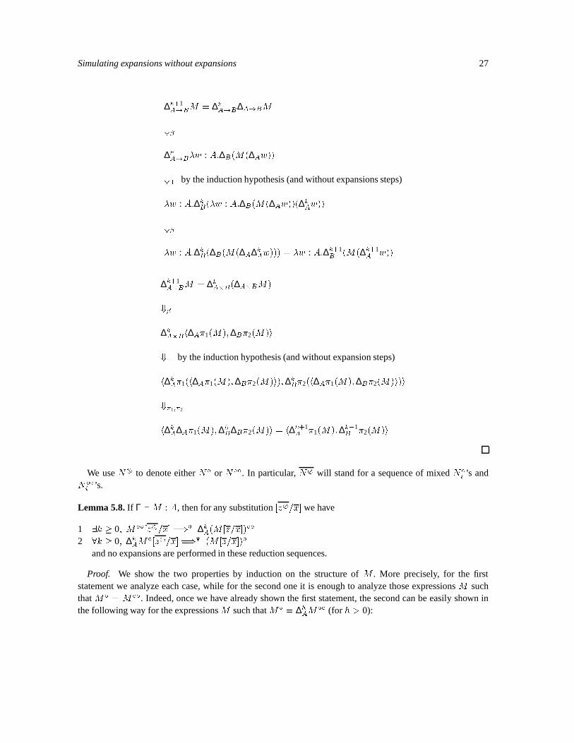
Simulating expansions without expansions 27
∆k+1A!BM = ∆kA!B∆A!BM+�∆kA!B�w : A:∆B(M(∆Aw))++ by the induction hypothesis (and without expansions steps)�w : A:∆kB(�w : A:∆B(M(∆Aw))(∆kAw))+��w : A:∆kB(∆B(M(∆A∆kAw))) = �w : A:∆k+1B (M(∆k+1A w))
∆k+1A�BM = ∆kA�B(∆A�BM)+�∆kA�Bh∆A�1(M);∆B�2(M)i++ by the induction hypothesis (and without expansion steps)h∆kA�1(h∆A�1(M);∆B�2(M)i);∆kB�2(h∆A�1(M);∆B�2(M)i)i+�1;�2h∆kA∆A�1(M);∆kB∆B�2(M)i = h∆k+1A �1(M);∆k+1B �2(M)i
We use N to denote either N� or N��. In particular, N will stand for a sequence of mixed N�i ’s andN��i ’s.
Lemma 5.8. If Γ `M : A, then for any substitution [z=x] we have
1 9k � 0; M��[z=x] =)� ∆kA(M [z=x])��2 8k � 0; ∆kAM�[z=x] =)� (M [z=x])�
and no expansions are performed in these reduction sequences.
Proof. We show the two properties by induction on the structure of M . More precisely, for the firststatement we analyze each case, while for the second one it is enough to analyze those expressions M suchthat M� = M��. Indeed, once we have already shown the first statement, the second can be easily shown inthe following way for the expressions M such that M� = ∆hAM�� (for h > 0):

R. Di Cosmo and D. Kesner 28
∆kAM�[z=x] =∆kA∆hAM��[z=x] =)� (by the first statement)∆k+hA ∆mAM [z=x]�� = (as h > 0)M [z=x]�
Every reduction built in the following proof contains no expansion steps, as it is constructed from one-stepreductions that are not expansions or from reductions obtained by the induction hypothesis (and thus withoutexpansions) or from reductions obtained by lemma 5.7 (again without expansions). This remark will allow usto conclude that the reductions in the statements of the lemma contain no expansion.Now, let us analyze the first statement and the interesting cases of the second.
— M � �. Since � is of type T, ∆T is empty. We have���[z=x] = �[z=x] = � = ��� = ∆0T��� = ∆0T(�[z=x])��— M � xi 2 x. There are two cases to consider: either z = z� or z = z��.
– x��i [z=x] = xi[z=x] = z�i = ∆mA z��i = ∆mA (xi[z=x])��.
– x��i [z=x] = xi[z=x] = z��i = (xi[z=x])�� = ∆0A(xi[z=x])��.
— M � y 62 x. We have y��[z=x] = y[z=x] = y = ∆0Ay��.
— M � (PQ). We have (PQ)��[z=x] = (P ��Q�)[z=x] = P ��[z=x]Q�[z=x].By the induction hypothesis P ��[z=x] =)� ∆hB!AP [z=x]��– If h = 0, thenP ��[z=x]Q�[z=x]+� by the induction hypothesisP [z=x]��Q�[z=x]+� by the induction hypothesisP [z=x]��Q[z=x]� = (P [z=x]Q[z=x])�� = ((PQ)[z=x])�� = ∆0A(PQ[z=x])��– If h > 0, then:

Simulating expansions without expansions 29
∆hB!AP [z=x]��Q�[z=x]++ by lemma 5.7(�w : B:∆hA(P [z=x]��(∆hBw)))Q�[z=x]+�∆hA(P [z=x]��(∆hB(Q�[z=x])))+� by the induction hypothesis
∆hA(P [z=x]��Q[z=x]�) = ∆hA(P [z=x]Q[z=x])�� = ∆hA(PQ[z=x])��— M � �y : B:P .
1 for the first statement,
(�y : B:P )��[z=x] = (�y : B:P �)[z=x]=�y : B:P �[z=x]+� by the induction hypothesis�y : B:P [z=x]� = (�y : B:P [z=x])�� = ∆0B!C((�y : B:P )[z=x])��

R. Di Cosmo and D. Kesner 30
2 for the second statement,
∆kB!C(�y : B:P )�[z=x] = ∆kB!C(�y : B:P �)[z=x]=∆kB!C�y : B:P �[z=x]++ by lemma 5.7�w : B:∆kB((�y : B:P �[z=x])(∆kCw))+��w : B:∆kBP �[z=x][w�=y]+� by the induction hypothesis�w : B:(P [z=x][w=y])�=(�w : B:P [z=x][w=y])�=�(�y : B:P [z=x])� = ((�y : B:P )[z=x])�
— M � �i(P ), for i = 1; 2. �i(P )��[z=x] = �i(P ��)[z=x]=�i(P ��[z=x])+� by the induction hypothesis�i(∆hA1�A2(P [z=x]��)
– If h = 0, then�i(P [z=x]��) = �i(P [z=x])�� = ∆0Ai�i(P [z=x])�� = ∆0Ai(�i(P )[z=x])��– If h > 0, then �i(∆hA1�A2
(P [z=x])��)++ by lemma 5.7�i(h∆hA1�1((P [z=x])��);∆hA2
�2((P [z=x])��)i)+�i∆hAi�i((P [z=x])��) = ∆hAi�i(P [z=x])�� = ∆hAi(�i(P )[z=x])��
Simulating expansions without expansions 31
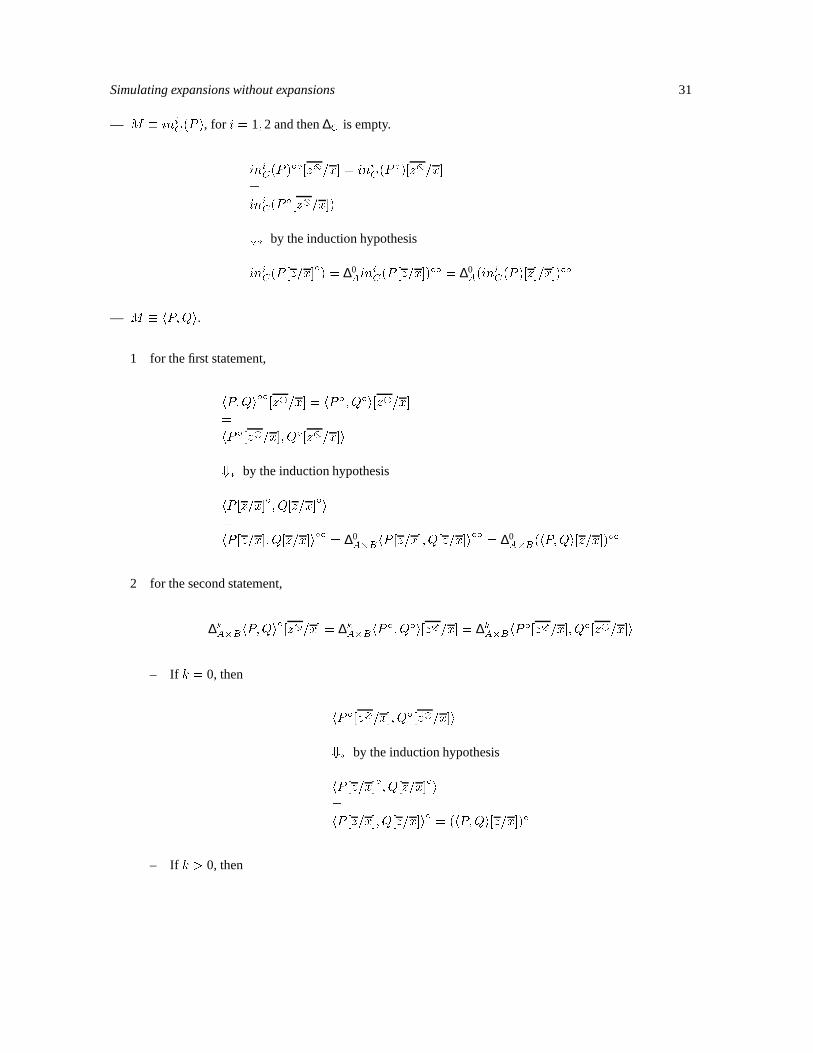
— M � iniC(P ), for i = 1; 2 and then ∆C is empty.iniC(P )��[z=x] = iniC(P �)[z=x]=iniC(P �[z=x])+� by the induction hypothesisiniC(P [z=x]�) = ∆0AiniC(P [z=x])�� = ∆0A(iniC(P )[z]=x])��— M � hP;Qi.
1 for the first statement,hP;Qi��[z=x] = hP �; Q�i[z=x]=hP �[z=x]; Q�[z=x]i+� by the induction hypothesishP [z=x]�; Q[z=x]�i=hP [z=x]; Q[z=x]i�� = ∆0A�BhP [z=x]; Q[z=x]i�� = ∆0A�B(hP;Qi[z=x])��2 for the second statement,
∆kA�BhP;Qi�[z=x] = ∆kA�BhP �; Q�i[z=x] = ∆kA�BhP �[z=x]; Q�[z=x]i– If k = 0, then hP �[z=x]; Q�[z=x]i+� by the induction hypothesishP [z=x]�; Q[z=x]�i=hP [z=x]; Q[z=x]i� = (hP;Qi[z=x])�– If k > 0, then

R. Di Cosmo and D. Kesner 32
∆kA�BhP �[z=x]; Q�[z=x]i++ by lemma 5.7h∆kA�1(P �[z=x]Q�[z=x]);∆kB�2(hP �[z=x]; Q�[z=x]i)i+� �1; �2h∆kAP �[z=x];∆kBQ�[z=x]i+� by the induction hypothesishP [z=x]�; Q[z=x]�i = hP [z=x]; Q[z=x]i� = (hP;Qi[z=x])�— M � (rec y : A:P )i.((rec y : A:P )i)��[z=x]=(rec y : A:P �)i[z=x]+� by the induction hypothesis(rec y : A:(P [z=x])�)i = ∆0A((rec y : A:P [z=x])i)�� = ∆0A((rec y : A:P )i[z=x])��— M � Case(P;Q;R). Case(P;Q;R)��[z=x] = Case(P �; Q�; R�)[z=x]=Case(P �[z=x]; Q�[z=x]; R�[z=x])+� by the induction hypothesisCase(P [z=x]�; Q[z=x]�; R[z=x]�)=Case(P [z=x]; Q[z=x]; R[z=x])��=(Case(P;Q;R)[z=x])��=
∆0A(Case(P;Q;R)[z=x])��Corollary 5.9. If Γ ` M : A, then 8k � 0; ∆kAM� =)� M� and no expansions are performed in thereduction sequences.
The following property is essential to show that every time we perform a �-reduction on a term M in theoriginal system, any translation of M reduces to a translation of the term we have obtained via !� from M .

Simulating expansions without expansions 33
Take for example the reduction (�x : A:M)N !� M [N=x]. We know that ((�x : A:M)N)� = ∆kA((�x :A:M�)N�) and we want to show that there is a non empty reduction sequence leading to M [N=x]�. Since∆kA((�x : A:M�)N�)!� ∆kAM�[N�=x], we have now to check that the term (M [N=x])� can be reached. Westate the property as follows:
Lemma 5.10. If Γ `M : A, then
1 9k � 0; M��[N=x] =)� ∆kA(M [N=x])��2 8k � 0; ∆kAM�[N=x] =)� (M [N=x])�
and no expansions are performed in the reduction sequences.
Proof. We show the two properties by induction on the structure of M . More precisely, for the firststatement one analyzes each case, while for the second one it is enough to analyze those expressions M suchthat M� = M��. Indeed, once we have already shown the first statement, the second can be easily shown inthe following way for the expressions M such that M� = ∆hAM�� (for h > 0):
∆kAM�[N=x] =∆kA∆hAM��[N=x] =)� (by the first statement)∆k+hA ∆mAM [N=x]�� =)� (either by definition of M [N=x]� or by corollary 5.9)M [N=x]�
Now, the analysis of all the cases involved proceeds exactly as in lemma 5.8, except for the case M � xi,where to prove the second statement we need to proceed as follows:
∆kAx�i [N=x] = ∆kA(∆mAxi)[N=x] = ∆k+mA NiNow, if Ni is N�i , by corollary 5.9, ∆k+mA N�i =)� N�i = (xi[N=x])� as required.
If instead Ni is N��i , we have two cases:
— N�i = N��i , then by corollary 5.9 ∆k+mA N�i =)� N�i = (xi[N=x])�.— otherwise, ∆k+mA N��i = N�i = (xi[N=x])�.
Notice that there are no expansions in these reduction sequences, because of corollary 5.9.
Lemma 5.11. If M�;�;Top�! N , then M�:�;:�=)+N�.
Proof.
— If M is of type A�B and M ��! h�1(M); �2(M)iWe know that 9k > 0 such that M� = ∆kA�BM��. By corollary 5.7
∆kA�BM��=)+ h∆kA�1(M��);∆kB�2(M��)iand the sequence has no expansion rules.The last term is equal to h�1(M)�; �2(M)�i = h�1(M); �2(M)i� and then the property holds.
— If M is of type A! B and M ��! �y : A:MyWe know that9k > 0 such that M� = ∆kA!BM��. By corollary 5.7 ∆kA!BM��=)+ �y : A:∆kB(M��(∆kAy))and the the sequence has no expansion rules.The last term is equal to �y : A:∆kB(M��y�) = �y : A:(My)� = (�y : A:My)� and then the propertyholds.
— If M : T and M Top�! �.By lemma 5.5 M� : T and so M� Top�! � = ��.

R. Di Cosmo and D. Kesner 34
Using 5.10 we can show now:
Theorem 5.12. (Simulation) If Γ `M : A and M =) N , then
1 9k � 0 such that M��=)+∆kAN�� if not M �;��! N2 M�=)+N�and there are no expansions in these reduction sequences.
Proof. We show the property by induction on the structure of M . More precisely, for the first statement weanalyze each case, while for the second there are two cases:
— if M �;��! N , then apply lemma 5.11— if not M �;��! N , then it is enough to analyze only the cases such that M� = M��, because whenM� = ∆hAM�� (for h > 0) we have easily:M� = ∆hAM��=)+ (by the first statement) ∆hA∆kAN�� = ∆h+kA N��
Then either N is not a pair nor a �-abstraction, which gives ∆h+kA N�� = N� because h > 0, or otherwise∆h+kA N�� = ∆h+kA N� =)� N� by lemma 5.9.
In order to conclude that the reductions in the statements of the lemma contain no expansions, it suffices tonotice that every reduction built in the following proof contains no expansion steps: indeed it is constructedfrom one-step reductions that are not expansions or from reductions obtained by the induction hypothesis (andthus without expansions) or from reductions obtained by lemma 5.11, lemma 5.7, (again without expansions).Now, we can analyze the cases involved in the proof of the first and the second statement.
— M � �. It is in normal form.— M � x. The only possible case is x Top�! �, where x : T. Then, x�� = x Top�! � = ∆0T���.— M � (P1Q1).
– If (P1Q1) : T and (P1Q1) Top�! �, then (P1Q1)�� : T by lemma 5.5 and then(P1Q1)�� Top�! � = ∆0T���– If (�x : C:R)Q1
��! R[Q1=x].((�x : C:R)Q1)�� = ((�x : C:R)��Q�1) = ((�x : C:R�)Q�
1) �=)R�[Q�1=x] =)� (by lemma 5.10) R[Q1=x]� = ∆kAR[Q1=x]��
– If (P1Q1) =) (P2Q1), where P1 =) P2.Since it is not the case thatP1
��! P2 because (P1Q1) =) (P2Q1), we have by the induction hypothesisa reduction sequence P ��
1 =)+ ∆hB!AP ��2 without expansions. Then(P1Q1)�� = P ��
1 Q�1=)+ (by ind. hyp.) (∆hB!AP ��
2 )Q�1
If h = 0, then (P ��2 Q�
1) = (P2Q1)��.

Simulating expansions without expansions 35
If h > 0, then (∆hB!AP ��2 )Q�
1++ by lemma 5.7(�w : B:∆hA(P ��2 (∆hBw)))Q�
1# �∆hA(P ��
2 (∆hBQ�1))+ � by corollary 5.9
∆hA(P ��2 Q�
1) = ∆hA(P2Q1)��– If (P1Q1) =) (P1Q2), where Q1 =) Q2(P1Q1)�� = P ��
1 Q�1=)+ (by ind. hyp.) P ��
1 Q�2 = (P1Q2)��
— M � hP1; Q1i– If hP1; Q1i =) hP2; Q1i, where P1 =) P2.
1 hP1; Q1i�� = hP �1 ; Q�
1i=)+ (by ind. hyp.) hP �2 ; Q�
1i = hP2; Q1i�� = ∆0AhP2; Q1i��2 Since hP;Qi�� = hP;Qi�, we have hP1; Q1i�=)+hP2; Q1i� by the previous statement.
– If hP1; Q1i =) hP1; Q2i, where Q1 =) Q2.
1 hP1; Q1i�� = hP �1 ; Q�
1i=)+ (by ind. hyp.) hP �1 ; Q�
2i = hP1; Q2i�� = ∆0AhP1; Q2i��2 Since hP;Qi�� = hP;Qi�, we have hP1; Q1i�=)+hP1; Q2i� by the previous statement.
— M � �x : A:P1
Then �x : A:P1 =) �x : A:P2, where P1 =) P2.
1 (�x : A:P1)�� = �x : A:P �1 =)+ (by ind. hyp.) �x : A:P �
2 = ∆0A!B(�x : A:P2)��2 Since (�x : A:Pi)� = (�x : A:Pi)�� we have (�x : A:P1)�=)+(�x : A:P2)� by the previous
statement.
— M � iniC(P1), for i = 1; 2 where P1 =) P2.Then iniC(P1) =) iniC(P2)iniC(P1)�� = iniC(P �
1 )=)+ (by ind. hyp.) iniC(P �2 ) = ∆0B+CiniC(P2)��
— M � �i(P1), for i = 1; 2.
– If �i(P1) : T and �i(P1) Top�! �, then �i(P1)�� : T by lemma 5.5 and �i(P1)�� Top�! � = ∆0Top���.
– If �i(P1) =) �i(P2), where P1 =) P2.Since it is not the case that P1
��! P2 because �i(P1) =) �i(P2), we have by the induction hypothesisa reduction sequence P ��
1 =)+ ∆hB�AP ��2 without expansions. Then�i(P1)�� = �i(P ��
1 )=)+ (by ind. hyp.) �i(∆hA1�A2P ��
2 )

R. Di Cosmo and D. Kesner 36
If h = 0, then �i(P ��2 ) = �i(P2)�.
If h > 0, then �i(∆hA1�A2P ��
2 )++ by lemma 5.7�i(h∆hA1�1(P ��
2 );∆hA2�2(P ��
2 )i)+�i∆hAi�i(P ��
2 ) = ∆hAi�i(P2)��— M � Case(P1; R1; N1)
– If Case(P1; R1; N1) : T and Case(P1; R1; N1) Top�! �, then Case(P1; R1; N1)�� : T by lemma 5.5and �i(P1)�� Top�! � = ∆0Top���.
– Case(iniC1+C2(S); R1; R2) ��! RiSCase(iniC1+C2
(S); R1; R2)�� =Case(iniC1+C2(S)�; R�1 ; R�2) =Case(iniC1+C2(S�); R�1 ; R�2) �=)R�1S� =(∆hCi!AR��1 )S�=)+ (by lemma 5.7)(�w : Ci:∆hA(R��1 (∆hCiw)))S� ��!
∆hA(R��1 (∆hCiS�)) =)� by corollary 5.9∆hA(R��1 S�) =∆hA(R1S)��
– Case(P1; R1; N1) =) Case(P2; R1; N1), where P1 =) P2.Case(P1; R1; N1)�� =Case(P �1 ; R�1 ; N�
1 )=)+ (by ind. hyp.)Case(P �2 ; R�1 ; N�
1 ) =Case(P2; R1; N1)�� =∆0ACase(P2; R1; N1)��
– Case(P1; R1; N1) =) Case(P1; R2; N1), where R1 =) R2Case(P1; R1; N1)�� =Case(P �1 ; R�1 ; N�
1 )=)+ (by ind. hyp.)Case(P �1 ; R�2 ; N�
1 ) =Case(P1; R2; N1)�� =∆0ACase(P1; R2; N1)��
– Case(P1; R1; N1) =) Case(P1; R1; N2), where N1 =) N2

Simulating expansions without expansions 37Case(P1; R1; N1)�� =Case(P �1 ; R�1 ; N�
1 )=)+ (by ind. hyp.)Case(P �1 ; R�1 ; N�
2 ) =Case(P1; R1; N2)�� =∆0ACase(P1; R1; N2)��
— M � (rec y : B:P1)i– If (rec y : T:P1)i : T and (rec y : T:P1)i Top�! �, then ((rec y : T:P1)i)�� : T by lemma 5.5 and((rec y : T:P1)i)�� Top�! � = ∆0Top���.
– (rec y : A:P1)i rec�! P1[(rec y : A:P1)i�1=y]((rec y : A:P1)i)�� =(rec y : A:P �1 )i rec�!P �
1 [(rec y : A:P �1 )i�1=y] =P �
1 [(rec y : A:P1)i�1��=y] =)� (by lemma 5.8)(P1[(rec y : A:P1)i�1=y])� =∆hA(P1[(rec y : A:P1)i�1=y])��
– (rec y : A:P1)i =) (rec y : A:P2)i.((rec y : A:P1)i)�� =(rec y : A:P �1 )i=)+ (by ind. hyp.)(rec y : A:P �2 )i =
∆0A((rec y : A:P2)i)��5.2. Strong Normalization of the Full Calculus
Having shown that our translation satisfies the hypothesis of Proposition 5.1, all we are now left to prove is thatthe bounded reduction system without expansion rules is strongly normalizing. This can be established by oneof the standard techniques of reducibility, and does not present essential difficulties once the right definitionsof stability or reducibility are given.
In 6 we provide a full proof, adapting Girard’s proof from (GLT90), but one can also adapt the proof providedby Poigne and Voss in (PV87), for which we just provide the basic definitions in 6.4. It is then finally possibleto state the following
Theorem 5.13. (Strong normalization)The reduction =) for the bounded system with expansions is strongly normalizing.
Proof. By proposition 5.1, theorem 5.12 and Corollary 6.7.
6. Strong Normalization without expansion rules
In this section we will prove the strong normalization property for our calculus ����� , with labeled recursion,but no expansions, using the reducibility method as in (GLT90), with an additional astute twist to take care ofthe sum type and labeled recursion.

R. Di Cosmo and D. Kesner 38
6.1. Reducibility
We define the set REDA of reducible terms of type A by induction on the type A as follows:
— For M of atomic type A, M 2 REDA iff M is strongly normalizable— For M of product type, M 2 REDA1�A2 iff �i(M) 2 REDAi— For M of a sum type, M 2 REDA1+A2 iff, for fresh variables wi : Ai, we haveCase(M;�x : A1:hx;w2i; �y : A2:hw1; yi) 2 REDA1�A2 (in the case Ai is T, we take � instead of wi)— For M of a functional type, M 2 REDA1!A2 iff for all N 2 REDA1 , (MN) 2 REDA2
Some comment on the sum type are needed here: first of all notice that the notion of reducibility is welldefined: reducibility for a sum type is given in term of reducibility for a product type, which has been definedbefore. Secondly, notice that for all other types, reducibility is either given directly as in the case of the basetypes, or given in terms of reducibility for types that are strictly smaller. This is not possible for the sum type,because we have no destructor associated to it, but only a case expression, so reducibility for A + B reallydepends on reducibility of A and B together, and we express this fact by reducing it to reducibility of theproduct A�B.
6.2. Properties of reducibility
Following (GLT90), we define a notion of neutrality: a term is neutral if does not interact with the surroundingcontext giving raise to redexes. In our case, the neutral terms are:� x �i(M) Case(P;M;N) (MN) (rec y:M)i
We will prove that REDA enjoys the following properties, for all types A:
(CR1) If M 2 REDA, then M is strongly normalizable.(CR2) If M 2 REDA, and M reduces to M 0, then M 0 2 REDA.(CR3) If M is neutral and whenever we perform on it one step of reduction we obtain a term M 0 2 REDA,
then M 2 REDA.As a special case of the last clause:
(CR4) If M is neutral and no reduction is applicable to it, then M 2 REDA.
In particular, � and the variables are reducible (also the variables of type T, as they can only reduce to �, whichis reducible).
Proposition 6.1. (Properties of reducibility) For every type A, the set REDA satisfies (CR1), (CR2) and(CR3).
Proof. We will proceed by induction on the type A.
6.2.1. Atomic types
(CR1) A reducible term of atomic type is strongly normalizable by definition(CR2) If M is strongly normalizable, then so is every reduct of M (as reduction preserves the type)(CR3) Suppose all one step reducts of M are reducible, i.e. strongly normalizable. Any reduction path leavingM must pass through one of its one-step reducts, which are in a finite number, so that the longest reduction
sequence starting from M has length the maximum among the 1+ �(M 0), as M 0 varies over the (one-step)reducts of M . Since these lengths are all finite, M is strongly normalizing.

Simulating expansions without expansions 39
6.2.2. Product types
(CR1) Suppose M 2 REDA1�A2 . Then by definition we know that �i(M) are reducible and so stronglynormalizing by the induction hypothesis. This implies that M is strongly normalizing also, because anyreduction sequence starting from M can be turned into a reduction sequence starting from �i(M).
(CR2) We know that �i(M) 2 REDAi , by definition. Now consider the possible one step reducts of M :
— M reduces toM 0. Then also �i(M) reduces to �i(M 0) via the same reduction, andM 0 is then reducibleby definition
(CR3) Let now M be neutral (not necessarily reducible) such that all its one step reducts are reducible. Wemust show that �i(M) is reducible of type Ai. Since M cannot be a pair (as it is neutral), any one stepreduction of �i(M) must be to a term �i(M 0), with M 0 one step from M . By (CR2), M 0 is reducible, andthen by definition also �i(M 0) is reducible. Now, �i(M) is neutral and all its one step reducts are reducible,hence by the induction hypothesis (CR3) for Ai, �i(M) is reducible, hence M is, by definition.
6.2.3. Arrow types
(CR1) Suppose M 2 REDA1!A2 . Then by definition we know that MN is reducible for all reducible N . Inparticular, Mx is reducible for a fresh variable x, which is reducible by the induction hypothesis (CR3) forA1, hence Mx is strongly normalizable. This implies that also M is strongly normalizing, as all reductionsequences starting from M can be performed also on Mx.
(CR2) Let M 2 REDA1!A2 reduce to M 0. For all N 2 REDA1 we have (M 0N) 2 REDA2 , since it is areduct of (MN), which is reducible because M and N are. Hence M 0 is reducible by definition.
(CR3) Let now M be neutral (not necessarily reducible) such that all one step reductions lead to reducibleterms. We show that MN is reducible for all reducible N by induction on �(N), using (CR3) for A2.Consider a one step reduction of MN : since M is neutral, this reduction must be either inside M or insideN and leads to:
— M 0N , with M 0 one step from M , so M 0 is reducible and hence M 0N is
— MN 0, with N 0 one step from N ; N 0 is reducible by (CR2) for A1, and �(N 0) < �(N), so by theinduction hypothesis MN 0 is reducible
Hence all reductions leaving MN lead to a reducible term and hence MN is reducible for all reducible N ,so that M is reducible by definition.
6.2.4. Sum types
(CR1) Suppose M 2 REDA1+A2 . Then by definition Case(M;�x:hx;w2i; �y:hw1; yi) 2 REDA1�A2 isreducible, hence strongly normalizable, hence M is strongly normalizable too.
(CR2) Suppose M 2 REDA1+A2 reduces to M 0. Then Case(M;�x:hx;w2i; �y:hw1; yi) 2 REDA1�A2
reduces to Case(M 0; �x:hx;w2i; �y:hw1; yi), so that, by (CR2) for A�B which has been proved before,Case(M;�x:hx;w2i; �y:hw1; yi) 2 REDA1�A2 . Hence M 0 is reducible too.(CR3) Let nowM be neutral, and suppose all its one step reducts are reducible. We will show thatCase(M;�x:hx;w2i; �y:hw1; yi)
(which is neutral) is reducible using (CR3) for A1 �A2, which has already been proved to hold. Considerthe possible one step reducts:
— Case(M 0; �x:hx;w2i; �y:hw1; yi) with M 0 one step fromM : thenM 0 is reducible, hence by definitionCase(M 0; �x:hx;w2i; �y:hw1; yi) is reducible
— there is no other one step reduct as M is neutral and the terms �x:hx;w2i and �y:hw1; yi are normal

R. Di Cosmo and D. Kesner 40
6.3. Reducibility theorem
We are left to show a few more lemmas:
Lemma 6.2. (Pairing) Let M1 : A1, M2 : A2 be reducible terms. Then hM1;M2i 2 REDA1�A2 .
Proof. We need to show that �i(hM1;M2i) 2 REDAi .Since �i(hM1;M2i) is neutral, we prove the statement using (CR3): we will show that all one step reductionsare reducible. We proceed by induction on the sum �(M1) + �(M2) of the maximum reduction lengths for M1
and M2, (which are finite, as these terms are strongly normalizable by (CR1)).The possible reducts are:
— Mi, which is reducible by hypothesis— �i(hM 0
1;M2i): now, M 01 is one step from M1, so that �(M 0
1) + �(M2) < �(M1) + �(M2), and M 01 is
reducible by (CR2), so �i(hM 01;M2i) is reducible by the induction hypothesis
— �i(hM1;M 02i): this is shown reducible as the term in the previous case
Lemma 6.3. (Abstraction) Let M : A2 be a term where the variable x : A1 may occur free. If for everyN 2 REDA1 we have M [N=x] 2 REDA2 , then �x : A1:M 2 REDA1!A2 .
Proof. We want to show that (�x:M)P is reducible for all reducible P . Since this term is neutral, we canprove our Lemma using (CR3). We are then left to show that all one step reducts of (�x:M)P are reducibleif for all N 2 REDA1 we have M [N=x] 2 REDA2 . Since M = M [x=x] is reducible by hypothesis (as anyvariable is reducible), it is strongly normalizable by (CR1), and we can proceed to prove this last statement byinduction on �(M) + �(P ). The term (�x:M)P converts to:
— M [P=x] which is reducible by hypothesis— (�x:M 0)P with M 0 a reduct of M ; now, by (CR2),M 0 is still reducible and furthermore �(M 0)+ �(P ) <�(M)+�(P ) andM [P=x] reduces toM 0[P=x], and this last term is also reducible, because it is a multi-step
reduct of M [P=x] by Lemma 4.5. So the induction hypothesis tells us that (�x:M 0)P is reducible.— (�x:M)P 0 with P 0 a reduct of P ; now, by (CR2), P 0 is still reducible and furthermore �(M) + �(P 0) <�(M) + �(P ) and M [P=x] reduces to M [P 0=x], by Corollary 4.8, so this last term is also reducible. The
induction hypothesis tells us that (�x:M)P 0 is reducible.
Lemma 6.4. (Injections) For all terms, M 2 REDA1 iff iniA1+A2(M) 2 REDA1+A2 .
Proof. ())We must show thatCase(iniA1+A2
(M); �x:hx;w2i; �y:hw1; yi) is reducible of typeA1�A2, i.e. that�i(Case(iniA1+A2(M); �x:hx;w2i; �y:hw ; yi)) 2REDAi . We will proceed using (CR3), by induction on �(M), because�i(Case(iniA1+A2
(M); �x:hx;w2i; �y:hw1; yi))is neutral.Consider then all its one step reducts:
— ((�x:hx;w2i)M), which is reducible because M is reducible and �x:hx;w2i is reducible (by Lemma 6.2applied to the variables x and w2 we know that hx;w2i is reducible, and we get reducibility of �x:hx;w2iby Lemma 6.3; similarly if we have � instead of w2)
— �i(Case(iniA1+A2(M 0); �x:hx;w2i; �y:hw1; yi)) withM 0 one step fromM , hence reducible and �(M 0) <�(M), so that it is reducible by the induction hypothesis

Simulating expansions without expansions 41
(()Suppose now, iniA1+A2
(M) 2 REDA1+A2 . This means, by definition of reducibility over sum types,Case(iniA1+A2(M); �x:hx;w2i; �y:hw1; yi) 2 REDA1�A2 ;
which implies, by definition of reducibility over product types,�1(Case(iniA1+A2(M); �x:hx;w2i; �y:hw1; yi)) 2 REDA1
This term reduces to �1((�x:hx;w2iM)), which in turn reduces to �1(hM;wi) and then to M , which is thenreducible by repeated use of (CR2).
Lemma 6.5. (Sum) Let P : A+B,M : A! C and N : B ! C be reducible terms. Then Case(P;M;N) 2REDC .
Proof. We will work by cases on C.
C is an atomic type We can use (CR3) for C, as Case(P;M;N) is neutral. We will show by induction on�(P )+ �(M)+ �(N) that all one step reducts of Case(P;M;N) are reducible. Consider the possible onestep reducts:
— Case(P 0;M;N), or Case(P;M 0; N), or Case(P;M;N 0): they are reducible by the induction hy-pothesis as all primed terms are reducible by (CR2) on A + B, A ! C, B ! C, and the measuredecreases strictly.
— (RM) if P � iniA1+A2(R): then R is also reducible by Lemma 6.4, and this term is reducible as M isC � C1 � C2 We must show �i(Case(P;M;N)) 2 REDCi . Since �i(Case(P;M;N)) is neutral, we can
use (CR3) for Ci. Since P , M , N , are all reducible, they are all strongly normalizable and we can proceedby induction on the measure �(P ) + �(M) + �(N). Consider the possible one step reducts:
— �i(Case(P 0;M;N)) or �i(Case(P;M 0; N)) or �i(Case(P;M;N 0)): they are reducible by the in-duction hypothesis as all primed terms are reducible by (CR2) on A + B, A ! C, B ! C, and themeasure decreases strictly.
— �i((MR)) if P � iniA1+A2(R): then R is also reducible by Lemma 6.4, so MR is reducible and�i((MR)) tooC � C1 ! C2 We must show Case(P;M;N)Q 2 REDC2 for all Q 2 REDC1 . Since Case(P;M;N)Q is
neutral, we can use (CR3) for C2. Since P , M , N , Q are all reducible, they are all strongly normalizableand we can proceed by induction on the measure �(P ) + �(M)+ �(N)+ �(Q). Consider the possible onestep reducts:
— Case(P 0;M;N)Q, or Case(P;M 0; N)Q, or Case(P;M;N 0)Q, or Case(P;M;N)Q0: they are re-ducible by the induction hypothesis as all primed terms are reducible by (CR2) on A + B, A ! C,B ! C and C1, and the measure decreases strictly.
— (RM)Q if P � iniA1+A2(R): then R is also reducible by Lemma 6.4, and this term is reducible as M
and Q areC � C1 + C2 We must show Case(Case(P;M;N); �x:hx;w2i; �y:hw1; yi) 2 REDC1�C2 . We can use(CR3) for C1 � C2 because Case(Case(P;M;N); �x:hx;w2i; �y:hw1; yi) is neutral. Since P , M , N ,are all reducible, they are all strongly normalizable and we can proceed by induction on the measure�(P ) + �(M) + �(N). Consider the possible one step reducts:

R. Di Cosmo and D. Kesner 42
— Case(Case(P 0;M;N); �x:hx;w2i; �y:hw1; yi) orCase(Case(P;M 0; N); �x:hx;w2i; �y:hw1; yi) orCase(Case(P;M;N 0); �x:hx;w2i; �y:hw1; yi): they are reducible by the induction hypothesis as allprimed terms are reducible by (CR2) on A+B, A! C, B ! C, and the measure decreases strictly.
— Case((RM); �x:hx;w2i; �y:hw1; yi) if P � iniA1+A2(R): thenR is also reducible by Lemma 6.4, and
this term is reducible by definition as M , hence also (RM), is
We will now prove that every reducible instance of a (not necessarily reducible) term M is reducible. As aconsequence, all terms will be reducible.
Theorem 6.6. (Reducibility) Let M be any term (not assumed to be reducible), and suppose all the freevariables of M are among x1; : : : xn of types A1; : : : An. If N1; : : :Nn are reducible terms of types A1; : : : An,then M [N=x] is reducible.
Proof. By induction on the structure of M .
1 M is �. It is neutral and normal, so it is reducible.2 M is xi for some i, then M [N=x] = Ni is reducible3 M � �i(M 0). By the induction hypothesis, M 0[N=x] is reducible, hence, by definition, �i(M 0[N=x]) =�i(M 0)[N=x] is reducible.4 M � hM1;M2i. By the induction hypothesis, the terms Mi[N=x] are reducible, so we conclude that the
term hM1[N=x];M2[N=x]i = hM1;M2i[N=x] is reducible.5 M � iniA1+A2
(M 0). By the induction hypothesis, M 0[N=x] is reducible, hence by Lemma 6.4, we havethat iniA1+A2
(M 0[N=x]) = iniA1+A2(M 0)[N=x] is reducible.
6 M � Case(M1;M2;M3). By the induction hypothesis, the terms Mi[N=x] are reducible, hence we havethat Case(M1[N=x];M2[N=x];M3[N=x]) = Case(M1;M2;M3)[N=x] is reducible.
7 M � (M1M2). By the induction hypothesis, the terms Mi[N=x] are reducible, so we conclude that theterm (M1[N=x]M2[N=x]) = (M1M2)[N=x] is reducible.
8 M � �y:M 0. Then by the induction hypothesis M 0[N=x][N 0=y] is reducible for all reducible terms N 0.By Lemma 6.3, �y:M 0[N=x] = (�y:M 0)[N=x] is reducible.
9 M � (recy:M 0)i. By the induction hypothesis, M 0[N=x] is reducible. We will show reducibility for(recy:M 0)i[N=x] by induction on i+ �(M 0). Since (recy:M)i[N=x] is neutral, we will use (CR3) for thetype A of (recy:M)i. Consider the one step reducts of (recy:M)i[N=x]— (recy:M 00)i[N=x] with M 00 one step from M 0. Then M 00[N=x] is reducible for all reducible
�!N ,because it is a multi-step reduct of the reducible termM 0[N=x] (Lemma 4.5). Furthermore,i+�(M 00) <i+ �(M 0), so by the induction hypothesis (recy:M 00[N=x])i = (recy:M 00)i[N=x] is reducible.
— M 0[N=x][(recy:M 0[N=x])i�1=y]. Then (recy:M 0)i�1[N=x] = (recy:M 0[N=x])i�1 is reducible bythe induction hypothesis, and this tells us that [N=x][(recy:M 0[N=x])i�1=y] is a substitution of re-ducible terms for a set of variables containing the free variables of M 0, which gives us reducibility ofthe term M 0[N=x][(recy:M 0[N=x])i�1=y].
Corollary 6.7. (Strong Normalization) All terms are reducible, hence strongly normalizable.

Simulating expansions without expansions 43
6.4. Another method
It is also possible to adapt a proof based on the notion of stability, as the one provided by Poinge and Voss. Wejust give here the basic definition, and refer the interested reader to (DCK93b) for full details.
6.5. Stability
We define a set of stable terms of type A by induction on the type A in the following way:
— For M of atomic type A, M is stable if and only if it is strongly normalizing.
— For M of type A1 � A2, M is stable if and only if it is strongly normalizing and whenever M reduces tohM1;M2i, then M1 and M2 are stable terms of type A1 and A2 respectively.
— For M of type A1 + A2, M is stable if and only if it is strongly normalizing and whenever M reduces toiniA1+A2(M 0) then M 0 is stable of type Ai.
— For M of type A1 ! A2, M is stable if and only if for every stable term N of type A1, MN is a stableterm of type A2.
7. Confluence of the Full Calculus
In this section we deduce the confluence property for the calculus with bounded recursion as well as for theversion with unbounded recursion.
We can immediately deduce the confluence property for the bounded system from the weak confluence andstrong normalization properties using Newman’s Lemma, however, we can also provide an extremely simpleand neat proof that does not need the weak confluence property for the expansionary system.
Theorem 7.1. (Confluence) The relation =) is Church-Rosser.
Proof. Since =) is weakly confluent by theorem 4.11 and strongly normalizing by theorem 5.13 we canconclude that it is Church Rosser by the well known Newman’s lemma.The other proof of confluence proceeds as follows.Let M be a term s.t. P1
�(= M =)� P2. Since =) is strongly normalizing, we can reduce the terms Pito their normal forms Pi. Then we have P1
�(= M =)� P2, and by theorem 5.12 P1� +(=M�=)+P2
�without expansions in the reduction sequences. As the system without expansions is confluent (we showed thatit is strongly normalizing, and weak confluence without expansions can be shown as easily as for the simplytyped lambda calculus), we can close the internal diagram with P1
� =)� R �(= P2�. Now,Pi� =lemma 5:6 Pi
and therefore we can complete the proof using the reductions P1 =)� P1 =)� R �(= P2�(= P2 (notice
that P1 = R = P2). The following figure shows the reduction diagram:

R. Di Cosmo and D. Kesner 44M�� ��� @@� @@RP1 P2_� _�P1 M� P2� �� ��� @@� @@R �P2� P2
�@@� @@R �� ���RIn order to show confluence of the full calculus we relate in the first place the bounded reduction =) and
the unbounded one1=) , and then we use the confluence of =) to show the confluence of
1=) . This verysame technique, that originates from early work of Levy (Lev76), was used in (PV87). The connection betweenthe reductions =) and
1=) comes from the following:
Remark 7.2. If M =)� N , then jM j 1=) jN j, where jM j is obtained from M by removing all the indicesfrom the rec terms.
Lemma 7.3. For any reduction sequence M01=)M1
1=) : : : 1=)Mn, there exists an indexed computationN0 =) N1 =) : : : =) Nn such that jNij = Mi, for i = 0 : : : n.
Proof. Index all the rec constructors in M0 by a number n+ k, with k � 0.
Confluence of the full calculus results now from the confluence of the bounded calculus.
Theorem 7.4. 1=) is Church Rosser.
Proof. Let M � P01=) P1
1=) : : : 1=) Pn and M � Q01=) Q1
1=) : : : 1=) Qm. By lemma 7.3P 00 =) P 0
1 =) : : : =) P 0n and Q00 =) Q0
1 =) : : : =) Q0m are indexed computations, where jP 0i j = Pi,for i = 0 : : : n and jQ0ij = Qi, for i = 0 : : :m.We can assume thatP 0
0 � Q00 by indexingP 0 andQ0 withn+m. As =) is Church Rosser by theorem 7.1, there
exists a term R such that P 0n =)� R and Q0m =)� R. By 7.2 Pn = jP 0nj 1=)� jRj and Qm = jQ0mj 1=)� jRj.8. Adding weak extensionality for the sum type
In this section we show how to apply our techniques in order to accommodate in our system the weakextensionality for the sum type, that is described by the following equality, which tells us that any term P ofsum type A1 +A2 is definitely an injection from one of the two types Ai.Case(P; �x:in1(x); �y:in2(y)) = P (1)
This is the usual equality that is found in proof theory, associated to the logical connective for disjunction

Simulating expansions without expansions 45
(see for example (GLT90; Gir72)). We call this rule “weak” because in category theory there is another strongerkind of extensional equality associated to the sum, that is used to axiomatize the uniqueness of the sum of twoarrows in the diagram for the coproduct, namelyCase(P;M � �x:in1(x);M � �y:in2(y)) = MP (2)
where M �N is the usual abbreviation for the composition �x:(M(Nx)).One can easily see that this strong rule really breaks down into two simpler rules: the weak rule 1 we just
introduced and the following commutation rule:Case(P;M �N1;M �N2) = MCase(P;N1; N2) (3)
If one really wants the equality 2, it seems to be a difficult task to provide a confluent system for theextensional theory with arrow, product and coproduct types, as discussed in (Dou90), and to the author’s bestknowledge, there are no positive results in that direction.
Notice also that the equation 1 can be easily added to a reduction system with no T type, where all theextensional equalities are turned into contractions, as done for example in (Gal93). In the presence of the Ttype, to use contraction rules one is forced to proceed along the lines of (CDC91), and to generate an infiniteset of reduction rules.
It is not obvious to add weak extensionality for the sum to our system, as the naıve idea of adding theequality 1 as a contraction rule breaks confluence, as the following example shows:Case(w; �x : A! B:in1(A!B)+C(x); �y : C:in2(A!B)+C(y)) =======) wk+Case(w; �x : A! B:in1(A!B)+C(�z : A:xz); �y : C:in2(A!B)+C(y))
This problem comes from the fact that the term �x : A! B:in1(A!B)+C(x) is not in normal form w.r.t. the
rules �, � and Top. This also suggests the solution: it suffices to completely expand the terms IN 1 = �x:in1(x)and IN 2 = �y:in2(y) w.r.t. the rules �, � and Top (which we know now are strongly normalizing) beforeperforming the contraction for the weak sum extensional equality.
So we are led to consider the contraction rule:Case(P; kIN 1k; kIN 2k) +�! Pwhere kMk denotes the normal form of M w.r.t. �, � and Top expansions.It is now straightforward to check that the weak confluence property still holds, and one is left to check that
the simulation theorem stays valid.For that, we have to verify that Case(P; kIN 1k; kIN 2k)�=)+P � without using expansion rules in the
reduction sequence, and this is obtained by:Case(P; kIN 1k; kIN 2k)� =∆kA+BCase(P �; kIN 1k�; kIN 2k�) =∆kA+BCase(P �; kIN 1k; kIN 2k) +=)∆kA+BP � =)�P �

R. Di Cosmo and D. Kesner 46
Notice that the rules �, � and Top do not create new redexes, as shown in lemma 3.7, so in particular kIN ikis still in normal form, and the equality kIN ik� = kIN ik can be obtained from lemma 5.6.
9. Conclusions
We have provided a confluent rewriting system for an extensional typed �-calculus with product, sum, terminalobject and recursion, which is also strongly normalizing in case the recursion operator is bounded. Thereare mainly two relevant technical contributions in this paper: the weak confluence proof and the simulationtheorem.
On one hand, let us remark once again that the weak confluence property for a context-sensitive reductionsystem is not as straightforward as for the reduction systems that are congruencies. The proof is no longer justa matter of a boring but trivial case analysis, so we had to explore and analyze here the fine structure of thereduction system, showing clearly how substitution and reduction interact in the presence of context-sensitiverules.
The simulation theorem, on the other hand, turns out to be the real key tool for this expansionary system:it allows to reduce both confluence and strong normalization properties to those for the underlying calculuswithout expansions, that can be proved using the standard techniques. In a sense, this is all that you really needto prove.
References
Y. Akama. On mints’ reductions for ccc-calculus. In M. Bezem and J. Groote, editors, Typed Lambda Calculus andApplications, volume 664 of LNCS, pages 1–12. Springer Verlag, 1993.
H. Barendregt. The Lambda Calculus; Its syntax and Semantics (revised edition). North Holland, 1984.P.-L. Curien and R. Di Cosmo. A confluent reduction system for the �-calculus with surjective pairing and terminal object.
In Leach, Monien, and Artalejo, editors, Intern. Conf. on Automata, Languages and Programming (ICALP), number 510in LNCS, pages 291–302. Springer-Verlag, 1991.
H. Curry and R. Feys. Combinatory Logic, volume 1. North Holland, 1958.D. Cubric. On free ccc. Distributed on the types mailing list, 1992.R. Di Cosmo and D. Kesner. A confluent reduction for the extensional typed ��calculus with pairs, sums, recursion
and terminal object. In A. Lingas, editor, Intern. Conf. on Automata, Languages and Programming (ICALP), LNCS.Springer-Verlag, 1993.
R. Di Cosmo and D. Kesner. Simulating expansions without expansions. Technical Report LIENS-93-11/INRIA 1911,LIENS-DMI and INRIA, 1993.
D. J. Dougherty. Some reduction properties of a lambda calculus with coproducts and recursive types. Technical report,Wesleyan University, 1990. E-mail: [email protected].
D. J. Dougherty. Some lambda calculi with categorical sums and products. In Proc. of the Fifth International Conferenceon Rewriting Techniques and Applications (RTA), 1993.
J. Gallier. On the correspondence between proofs and �-terms. Available by anonymous ftp from ftp.cis.upenn.edu.Author’s address: [email protected]., January 1993.
J.-Y. Girard. Interpretation fonctionelle et elimination des coupures dans l’arithmetique d’ordre superieure. These dedoctorat d’etat, Universite de Paris VII, 1972.
J.-Y. Girard, Y. Lafont, and P. Taylor. Proofs and Types. Cambridge University Press, 1990.G. Huet. Resolution d’equations dans les langages d’ordre 1; 2; : : : ; !. These d’Etat, Universite Paris VII, 1976.C. B. Jay. Long �� normal forms and confluence (and its revised version). Technical Report ECS-LFCS-91-183, LFCS,
University of Edimburgh, 1992.

Simulating expansions without expansions 47
C. B. Jay and N. Ghani. The virtues of eta-expansion. Technical Report ECS-LFCS-92-243, LFCS, University of Edimburgh,1992.
J. W. Klop. Combinatory reduction systems. Mathematical Center Tracts, 27, 1980.J.-J. Levy. An algebraic interpretation of the ���-calculus and a labelled �-calculus. Theoretical Computer Science,
2:97–114, 1976.J. Lambek and P. J. Scott. An introduction to higher order categorical logic. Cambridge University Press, 1986.G. Mints. Closed categories and the theory of proofs. Zapiski Nauchnykh Seminarov Leningradskogo Otdeleniya Matem-
aticheskogo Instituta im. V.A. Steklova AN SSSR, 68:83–114, 1977.G. Mints. Teorija categorii i teoria dokazatelstv.I. Aktualnye problemy logiki i metodologii nauky, pages 252–278, 1979.G. Pottinger. The Church Rosser Theorem for the Typed lambda-calculus with Surjective Pairing. Notre Dame Journal of
Formal Logic, 22(3):264–268, 1981.D. Prawitz. Ideas and results in proof theory. Proceedings of the 2nd Scandinavian Logic Symposium, pages 235–307,
1971.A. Poigne and J. Voss. On the implementation of abstract data types by programming language constructs. Journal of
Computer and System Science, 34(2-3):340–376, April/June 1987.A. S. Troelstra. Strong normalization for typed terms with surjective pairing. Notre Dame Journal of Formal Logic, 27(4),
1986.