size and shape in biology and shape in biology 3 variation in surface area to volume ratios. one of...
TRANSCRIPT

Association for Biology Laboratory Education (ABLE) ~ http://www.zoo.utoronto.ca/able 1
Chapter 1
Size and Shape in Biology
Thomas F. Colton*
Biological Sciences Collegiate Division The University of Chicago
924 E. 57th Street Chicago, IL 60637-5415
*Current address: University of California, Berkeley
Department of Integrative Biology 3060 Valley Life Sciences Building # 3140
Berkeley CA 94720-3140 Phone: (510) 642-3549
[email protected] Tom Colton received a B.A. in biology from the State University of New York at Binghamton, in 1977 and a Ph.D. in Zoology from Duke University in 1983. Since then he has taught at Duke University, the University of North Carolina at Greensboro, and Wake Forest University. As a senior lecturer at the University of Chicago since 1991, he teaches labs in biological diversity, physiology, and biomechanics, lectures in a biology course for non-majors, and directs the web site for the undergraduate biology program.
© 1999 The University of Chicago
Contents
Reprinted From: Colton, T. F. 1999. Diversity of photosynthetic pigments. Pages 1-44, in Tested studiesfor laboratory teaching, Volume 20 (S. J. Karcher, Editor). Proceedings of the 20th Workshop/Conference ofthe Association for Biology Laboratory Education (ABLE), 399 pages.
- Copyright policy: http://www.zoo.utoronto.ca/able/volumes/copyright.htm
Although the laboratory exercises in ABLE proceedings volumes have been tested and due consideration has been given to safety, individuals performing these exercises must assume all responsibility for risk. The Association for Biology Laboratory Education (ABLE) disclaims any liability with regards to safety in connection with the use of the exercises in its proceedings volumes.

2 Size and Shape in Biology
Introduction....................................................................................................................2 Materials ........................................................................................................................3 Notes for the Instructor ..................................................................................................4 Student Outline ..............................................................................................................5
Overview..................................................................................................................5 Background..............................................................................................................5 Scaling Exercises .....................................................................................................6
Scaling Exercise 1: Mussel Shells .....................................................................7 Scaling Exercise 2: Stress and the Human Foot ................................................8 Scaling Exercise 3: Ruminant Jaws ...................................................................11 Scaling Exercise 4: Cat Jaws .............................................................................14 Scaling Exercise 5: The Cat Cranium................................................................17 Scaling Exercise 6: Dog and Wolf Skulls..........................................................19 Scaling Exercise 7: Mammalian Femurs ...........................................................21
Using StatView 4.5 to Analyze Scaling Data ..........................................................22 Acknowledgements........................................................................................................24 Literature Cited ..............................................................................................................24 Appendix A: Pre-Lab Tutorial .......................................................................................26 Appendix B: Notes and Expected Results for Each Exercise........................................37
Introduction This is the first lab in a biological diversity course for second-year biology majors at the University of Chicago, though I developed it originally for a non-majors course on the biology of motion. This lab might also be appropriate for courses in anatomy, biomechanics, and evolutionary biology. The goals of this lab are to
(1) stimulate students to think about the implications of size for an organism's form and function as they encounter various phyla in subsequent labs,
(2) provide experience working in groups to develop hypotheses, take measurements, analyze data, and present results orally,
(3) teach the use of linear regression to describe patterns and test hypotheses, and (4) introduce the concepts of isometric and allometric scaling, the relationship of body size
to stress on skeletal elements, the use of lever mechanics to analyze musculo-skeletal systems, the scaling of brain size with body size, and the role of heterochrony in evolution.
Size has a profound influence on the shapes and functions of living organisms (Sweet
1980). Scaling, the study of the influence of body size on form and function, provides a useful tool for exploring differences in morphology among individuals and species (Biewener 1990, Gould 1977). Scaling has been applied also to understand physiological parameters, such as metabolic rate and heart rate (Schmidt-Nielsen 1984), and ecological parameters, including population sizes, biomass, home ranges, and population growth rates (Calder 1984, Peters 1983). Introductions to this topic suitable for students can be found in McMahon and Bonner (1983), Hildebrand (1995), McGowan (1994), and Vogel (1988). Instructors should consult two published lab exercises on allometry presented at earlier ABLE conferences (Goldman et al. 1990, Trombulak 1991), which differ from this exercise in methods and in their focus on

Size and Shape in Biology 3
variation in surface area to volume ratios. One of the most exciting aspects of this scaling exercise to students (and ABLE workshop participants) has been the precise fit of the data they collect to a simple power function, despite small sample sizes and, in some cases, comparisons across distantly-related species. The strength of the patterns they discover inspires a sense of remarkable consequence, even if the mechanisms responsible for generating the pattern are unclear. Prior to the lab period, students complete a web-based exercise (available on the ABLE web site and included below in Appendix A) and fill out a worksheet to hand in at the beginning of lab. With this background, students enter the lab prepared to apply the concepts of isometric and allometric scaling to their chosen exercise. During the 3-hour lab, each group of three students chooses one of the seven exercises in which to develop hypotheses, take measurements, and analyze data. Each of the six groups performs a different investigation and presents their results to the rest of the class orally, an opportunity to compare conclusions and learn from each other's projects. The group oral presentations are followed by individually-written formal lab reports due the following week. Each group uses a computer with StatView 4.5 software during the lab period for statistical analysis and graphing. This lab could be adapted to an open-ended inquiry-based format if it were spread over two lab periods (or a lecture and a lab) to allow time for students to develop their own questions. The seven exercises given below are intended as examples and inspiration; you may find even better ones by prospecting in your local teaching collections and field sites for specimens.
Materials
For Each Group (3 students) Computer with statistical analysis/graphing software (StatView 4.5) and access to a networked printer.

4 Size and Shape in Biology
Table 1.1 Materials by exercise.
Exercise Materials 1. Mussels assortment of shells
photos of mussels in habitat calipers electronic top-loading balance
2. Stress on the human foot bathroom scale tracings of children’s feet (& weights) to supplement
students’ data video camera and lens computer with A-V input and NIH-Image software
3. Ruminant jaws skulls of deer, muntjac, cattle, chevrotain calipers and large calipers
4. Cat jaws skulls (real or replicas) of domestic cat, clouded leopard, cougar, Siberian tiger, American lion, saber tooth cat
calipers large calipers
5. Cat cranium same specimens as (4) calipers large calipers
6. Dog and wolf skulls illustrations of growth series of great Dane skulls (real or replicas) of English bulldog, pug, Pekinese,
and others calipers
7. Mammalian femurs femurs or mounted skeletons of mouse, rat, chevrotain, cat, peccary, deer, bear, human, horse, Triceratops or Tyrannosaurus rex (cast)
calipers large calipers
Notes for the Instructor
Most of the biological specimens used in these exercises were collected in the field or borrowed from teaching and research collections. We purchased additional specimens to fill in gaps and expand the range of sizes. When selecting specimens for an exercise, I aim for at least a 3-fold difference in linear dimensions from the smallest to the largest specimen, though 10-fold is better. The sample size needed depends on the scatter in the data. Some of the relationships are so tight that a sample size of five is adequate, but ten specimens generally provides a reasonable estimate of the scaling exponent. To minimize breakage of the fragile and usually valuable mounted skeletons and skulls, we set them out on the lab benches at the station where each will be used and ask students not to remove them from the lab bench. If computers are not available in the lab room, then data could be analyzed later at a central computing facility, but this would preclude presenting the results during the lab period. Alternatively, the data could be plotted by hand on log-log graph paper and a line fitted by eye.
Size and Shape in Biology 5
The exercise on scaling of human feet can be performed without the video camera and A-V computer by cutting out the foot tracings and weighing them on a top-loading balance, or by measuring foot length and width. Students need considerable attention from the instructors during the hypothesis-development stage and the analysis stage. In the former, we ask students to be specific about the scaling exponent that corresponds to isometry and to specify a rationale for their predicted scaling exponent. One common difficulty in the analysis is using the 95% confidence intervals of the scaling exponent to test hypotheses. Beyond confusion about the procedure, many students become so emotionally attached to their hypotheses that they either refuse to believe contradictory statistics or feel themselves to be failures if their predictions are not fulfilled by the data. We try to convince students that results deviating from expectations can be a cause for excitement rather than embarrassment, as they often lead to innovation in science; we judge the appropriateness of their hypothesis by the reasoning that went into it, not by whether it survives the investigation.
Student Outline Overview
"You now see how, from the things demonstrated thus far, there clearly follows the impossibility (not only for art, but for nature herself) of increasing machines to immense size. Thus it is impossible to build enormous ships, palaces, or temples, for which oars, masts, beamwork, iron chains, and in sum all parts shall hold together; nor could nature make trees of immeasurable size, because their branches would eventually fail of their own weight; and likewise it would be impossible to fashion skeletons for men, horses, or other animals which could exist and carry out their functions proportionably when such animals were increased to immense height — unless the bones were made of much harder and more resistant material than the usual, or where deformed by disproportionate thickening, so that the shape and appearance of the animal would become monstrously gross."
Galileo Galilei, Two New Sciences (1638), as translated by Drake (1974:127)
Size, shape, and the relationships of each to function are important topics in organismal biology. Whether you are interested in understanding the significance of a particular morphology or interpreting the factors which may underlie a particular evolutionary trend, it is important that you understand the physical consequences and interdependence of organismal form and size. At best we can give you a basic understanding of the issues involved — the literature in this area is huge and spans topics from physiology to ecology — but even this basic treatment will give you powerful insights into the functional and structural consequences of size per se. In this lab you will take a sample of related biological specimens of different sizes, devise hypotheses about whether the shapes of these specimens vary with size and how that might relate to some biologically relevant function, and test your hypotheses by taking a series of measurements. The conceptual background for this lab is presented in a web-based tutorial which you should complete before coming to lab. The tutorial includes a worksheet which you should print out, complete, and hand in at the beginning of lab. The major concepts and equations presented in the tutorial are reviewed below.

6 Size and Shape in Biology
Summary of key concepts
Geometric Similarity: Two objects are considered geometrically similar if they have the same shape. For geometrically similar objects, one linear measure is proportional to another linear measure (e.g. if height is one half the diameter for one bowl, then all bowls with the same shape will show this relationship, no matter what their size). Other relationships include:
area α length2 (or length α area1/2) volume α length3 (or length α volume1/3) volume α area3/2 (or area α volume2/3)
Power Function: The relationships among various dimensions of objects of different sizes often can be represented by the equation
y = a xb
where x and y are two measures (such as a diameter and a surface area), b is the scaling exponent, and a is a constant that depends on shape The scaling coefficient, b, is a useful way to describe the relationship between the two measures, x and y. For geometrically similar objects, b will take on a value that is easily predicted from knowing whether x and y represent lengths, areas or volumes.
Isometric Scaling: This describes the condition where objects of different sizes share the
same shape. Objects or organisms that scale isometrically are geometrically similar. The relationship between any two size measures fits a power function with an easily-predicted scaling exponent, b.
Allometric Scaling: This describes a set of objects or organisms that differ in shape as well
as size. Objects that show allometric scaling are non-isometric and are not geometrically similar. The relationship between any two size measures may or may not fit a power function, but, if it does, the scaling exponent, b, will be different than that predicted by isometry.
Estimating the Scaling Exponent (b): To test whether organisms scale isometrically or
allometrically, two sets of anatomical measurements (x and y) can be fitted to the power function to determine the value of b. The simplest way to do this is to log - transform the measurements and perform a linear regression of log (y) on log (x), taking the slope as an estimate of b. A better (less biased) technique is the reduced major axis regression, which is the equivalent of dividing the slope of the regression by the correlation coefficient (r). If the value of b is equal to the prediction for isometry, then scaling is isometric. If the value of b is significantly different from the isometric prediction, then scaling is considered allometric.
Scaling Exercises In the following seven exercises, you will explore aspects of size and shape in biology by gathering some data of your own on specimens we will provide. Some of these specimens may scale isometrically, some may scale allometrically, and some may show both patterns depending

Size and Shape in Biology 7
on which sets of measurements you look at. We ask you to do only one of the following seven exercises; which one you do we leave to you to determine. The point of these exercises is for you to take some data from real biological specimens, determine the pattern of scaling, and finally to interpret your findings in biological terms. Later in the lab, each group will present their exercise to the rest of the class. Each individual will then write up the exercise he or she did to hand in next week. (Note that the latter assignment is an individual, not group, effort. Clearly the group will share the data, but the write-up should be your individual effort.) Scaling Exercise 1: Mussel Shells
I. The Organism The common blue mussel, Mytilus edulis: These shells were collected on the shores of
Campobello Island, New Brunswick, where they live attached by byssal threads (protein filaments that they secrete) to rocks and gravel low in the intertidal zone. Much of the space within the shell is occupied by the gill, which serves both to extract oxygen and to filter small food particles (mostly single-celled algae) from the water. Normally, the shell gapes open a few millimeters to allow water to be pumped through the gill, but the shells are closed tightly both during low tide (when the mussel is exposed to the air) and when the mussel is attacked by a predator. The different sizes of shells can be considered to represent different ages of the animals. Functions of the shell include preventing the animals from drying out when exposed at low tide and protection from predators such as a starfish, crabs, and birds. Mussels also face intense competition for space on the rocks from other mussels and from many other species of animals and algae.
II. Questions
1. As the mussel grows in size, does the overall shape of the shell change, and, if so, how? a. Does a power function describe the growth pattern? b. Is the growth isometric or allometric? c. What are some functional implications of shell shape?
2. As the mussel grows, how does the mass of the shell vary with length?
a. Does the shell mass grow isometrically or allometrically with respect to length? b. Does the shell become relatively more stout or lighter as its size increases? c. What are the functional implications of this relationship?
III. Your Hypotheses
IV. Methods 1. Choose two linear dimensions of the shell that can be determined consistently on all
specimens and use calipers to measure each of these. Draw a diagram of a shell and show the measurements you chose.

8 Size and Shape in Biology
2. Measure the mass of each shell on a top-loading electronic balance. Press the tare button to
zero the balance between weighings. V. Results
1. On one graph, plot the log of one linear dimension against the log of the other linear dimension. On a second graph, plot the log of shell mass on the y-axis against one of the linear dimensions on the x-axis.
2. Analyze the shapes of the curves (are they fairly straight lines, broken lines, or curves?) and
calculate the slopes (scaling exponent) if appropriate. 3. Attach your data table and graphs to your lab report, making sure to label columns and axes
and include units. Include the statistics you calculated and give the power function equation and scaling exponent (both least squares and reduced major axis estimates) for each graph. Use the 95% confidence interval of the scaling exponent to test whether the observed exponent was significantly different from your prediction or from isometry. VI. Conclusion
Write several paragraphs describing your findings, answering the initial questions, and explaining why you accept or reject your hypotheses. Discuss the functional implications for the animal of the relationships you found. Scaling Exercise 2: Stress and the Human Foot
I. The Organism
The human, Homo sapiens: This is a quite successful species that has recently experienced a dramatic increase in population size. Many attribute this success in part to the peculiar locomotion in this group — this species exclusively uses its hind limbs for locomotion, freeing up the fore limbs for manipulation and tool use. Although bipedal locomotion is common in birds and dinosaurs, it is extremely rare in mammals. One consequence of bipedal locomotion is that the entire body weight must be borne by the hind limbs. During walking, when the body is frequently supported by one foot, the stress can be calculated as
stress =forcearea
=mass( ) acceleration( )
area
where mass is the mass of the person (kg), acceleration is that due to gravity (9.8 m/second2), and area is the area of the foot (in cm2) in contact with the ground while standing. The units of stress we’ll use are Newtons/cm2.
II. Questions
1. How does foot area scale with body mass in humans? a. Does a power function describe the relationship between foot area and body mass? b. Is the growth isometric or allometric?

Size and Shape in Biology 9
c. What are some functional implications of this relationship?
2. As humans grow in size, does the stress on the feet change, and, if so, how?
III. Your Hypotheses
IV. Methods
1. Find a suitable sample of humans for your analysis. You'll want as broad a range of body sizes as possible. Dragoon your classmates into cooperating, or draw on the population wandering free in the building. If you can find a juvenile of the species, solicit his or her cooperation.
2. Measure the weight of each individual on the scale available in lab. 3. Have your subjects remove his or her shoes and trace the outline of one foot onto a piece of
clean white paper with a heavy black felt-tip marker. Draw a straight line of known length (say, 10 cm) to serve as a scale. Be sure to label the tracings so that you can correlate your weight measurements with measurements of foot area.
4. Measure the area of each tracing by digitizing a video image on the computer (see
instructions below).
Measuring Foot Area using a video camera and NIH Image software
To estimate foot area, you will digitize an image with a CCD video camera attached to a computer and measure the area using the image analysis program NIH Image. If you would like a free copy of this software or its documentation, it can be downloaded from the following URL: http://rsb.info.nih.gov/nih-image/
A. Capturing an image.

10 Size and Shape in Biology
1. Open the program NIH Image from the "Apple" menu on the far left of the menu bar by clicking on the apple, dragging down to "NIH Image", and releasing the mouse button.
2. From the File menu, drag down to the Acquire sub-menu and across to Plug-in Digitizer. A dialog box with an embedded image from the video camera should appear.
3. Adjust the focus and iris on the video camera. (After your first tracing, you shouldn’t need to repeat steps (1) - (3) as long as you don’t quit the program.)
4. To capture the image, click on the "OK" button (or click on “Freeze" and then "OK"). After several seconds, your image should appear.
5. Go to the Process menu and select Convert to Grayscale. This converts the color image to a black and white image with 254 levels of gray between white and black. (Do not use the "Grayscale" command in the Options menu.)
Figure 1.1 Tools you will need in NIH-Image.
B. Calibration.
1. On your first tracing, you should have drawn a heavy line of known length (say 10 cm). Click on the Line Selection Tool (dashed line icon) in the Tools window. Move the cursor to one end of this drawn line, click and drag to the other end of the line, and release the mouse button. The line should now appear as “marching ants”.
2. Go to the Analyze menu and select Set Scale. The length you have just indicated should appear (in units of pixels) in the Measured Distance box.
3. Click on the pop-up menu adjacent to the "Units" label and select the correct units (centimeters, millimeters, etc.).

Size and Shape in Biology 11
4. In the Known Distance box, type in the correct value (e.g., type "10" if the line you drew was 10 cm long) and click OK. You do not need to repeat this calibration for future tracings unless you quit the program or change the distance between the camera and tracing.
C. Measuring Area.
1. Under the Options menu, choose Threshold. 2. Move the cursor into the LUT (Look-up-table) window at the far left and drag the
black/white boundary up and down until the outline of the foot appears black against a white background. If there are any gaps in the tracing, use the Pencil tool to fill them in.
3. When the image is satisfactory, click on the Magic Wand in the Tools window (the line with a circle on its end just to the left of the eyedropper), position it just to the left of an edge of the foot, and click the mouse button. A line of "marching ants" should automatically outline your object.
4. Go to the Edit menu and choose Fill (to fill in the object with a uniform black). 5. Go to the Analyze menu, and choose Measure. The area of the foot has now been
measured. To view the result, choose Show Results in the Analyze menu. Each new measurement will appear at the bottom of the list.
6. When you’re done with an image, close it to avoid running out of memory. It is not necessary to save the images.
V. Results
1. Plot log (foot area) on the y-axis against log (body mass) on the x-axis. 2. Analyze the shape of the curve. (Is it a fairly straight line, a broken line, or a curve?)
Calculate the slope (scaling exponent) if appropriate. 3. Calculate the stress for each person’s foot. (Hint: Use StatView to do this by creating a new
column in the data set called “stress”, selecting source “dynamic formula”, and entering the formula in the popup menu.)
4. Attach your data table and graphs to your lab report, making sure to label columns and axes
and include units. Include the statistics you calculated and give the power function equation and scaling exponent (both least squares and reduced major axis estimates) for each graph. Use the 95% confidence interval of the scaling exponent to test whether the observed exponent was significantly different from your prediction or from isometry. VI. Conclusion
Write several paragraphs describing your findings, answering the initial questions, and explaining why you accept or reject your hypotheses. Discuss the functional implications for humans (and shoe manufacturers) of the relationship you found.

12 Size and Shape in Biology
Scaling Exercise 3: Ruminant Jaws
I. The Organisms
Deer, muntjac, chevrotain, and cattle: These animals are all ruminants, a suborder of the Order Artiodactyla, the even-toed, hoofed mammals. Ruminants eat coarse vegetation, such as leaves of grasses and trees, which are very difficult to digest because of tough fibers and the high cellulose content. After partially chewing the food, it is swallowed and fermented with cellulose-digesting bacteria in a stomach chamber called the rumen. The partially digested material (the cud) is then regurgitated and chewed further to release more nutrients and to increase the surface area of the vegetation so the bacteria can break it down more effectively. Grinding of the tough fibrous vegetation is accomplished with massively developed premolars and molars. The smallest ruminant, the chevrotain, or mouse deer, lives in the tropics of West Africa and Maylasia. The slightly larger muntjac lives in parts of India and China. Giraffes are also included in this group.
mandible jaw articulation
action of superficial masseter muscle
action of temporalis muscle
Figure 1.2. Action of major jaw muscles in a ruminant skull.
Jaw mechanics. Two muscles, the temporalis and the superficial masseter, originating on
the skull apply forces to the mandible in chewing. We will focus on the latter, which is most important in herbivores. The jaw can be viewed as a lever system for applying force to the food being chewed. A lever consists of a pivot point (the jaw articulation), and two lever arms. The in-lever arm connects the pivot to the point where an “in-force” (Fi) is applied by a muscle. The out-lever arm connects the pivot to the point where an “out-force” (Fo) is applied by the teeth to the food. As a general rule, the out-force can be increased by decreasing the out-lever arm and increasing the in-lever arm. The force-multiplying effect of a lever is characterized by the mechanical advantage:
The higher the mechanical advantage, the greater the out-force, or in this case, the chewing force. As a measure of the in-lever arm of the masseter we’ll use the distance from the jaw articulation to the bottom of the angular process, which we’ll call the Masseter In-Lever Arm, or
Mechanical Advantage= Fo Fi
= in lever-armout lever-arm

Size and Shape in Biology 13
MILA. As a measure of the out-lever arm for the chewing teeth, we’ll use the distance from the jaw articulation to the middle of the tooth row, which can be taken as the line between the 3rd premolar and 1st molar. We’ll call this the Chewing Out-Lever Arm, or COLA. The mechanical advantage can be calculated as the MILA/COLA.
out-lever arm
in-lever arm
Fi
Fo
premolars molars
COLA
MILA
angular process
Figure 1.3. Lever mechanics applied to a ruminant jaw.
II. Questions
1. Do the jaws of larger ruminants differ in shape from those of smaller ones? If so, how? 2. Does a power function describe the size-shape pattern? 3. Is the scaling of the jaws isometric or allometric? 4. How does mechanical advantage vary with size? 5. What are some functional implications of jaw shape?
III. Your Hypotheses
IV. Methods
Measure the MILA and COLA of each jaw with calipers or a ruler: V. Results
1. Plot the log (MILA) on the y-axis against the log (COLA) on the x-axis.

14 Size and Shape in Biology
2. Analyze the shape of the curve (is it a fairly straight line, broken line, or curve?) and calculate the slope (scaling exponent) if appropriate.
3. Calculate mechanical advantage for each jaw. (Hint: Use StatView by creating a new
column in the data set called “MA”, selecting source “dynamic formula”, and entering the formula in the popup menu.)
4. Attach your data table and graphs to your lab report, making sure to label columns and axes
and include units. Include the statistics you calculated and give the power function equation and scaling exponent (both least squares and reduced major axis estimates) for each graph. Use the 95% confidence interval of the scaling exponent to test whether the observed exponent was significantly different from your prediction or from isometry. VI. Conclusion
Write several paragraphs describing your findings, answering the initial questions, and explaining why you accept or reject your hypotheses. Discuss the functional implications for the animal of the relationships you found.
Scaling Exercise 4: Cat Jaws
I. The Organisms
Domestic cat, clouded leopard, cougar, Siberian tiger, saber tooth cat, American lion: These cats all belong to the Family Felidae, a group specialized as carnivores. This is evident in the teeth, which are specialized for biting (incisors), stabbing (canines), and slicing (premolars and molars), but quite incapable of grinding. Felids kill small prey with a bite at the back of the neck and larger prey with a neck bite that strangles the prey. The African lion and Siberian tiger are the largest living cats, but other large felids were dominant predators in North America in the past. The skulls you will examine include casts of two extinct species, the saber tooth cat and American lion, recovered from the La Brea tar pits in Los Angeles. The saber tooth cat is noted for its long upper canines (the “sabers”), which are believed to have been useful in stabbing and slicing large thick-skinned herbivores, such as mastodons. One theory about the extinction of large mammals in North America at the end of the Pleistocene attributes the decline of large herbivores like the mastodon to direct hunting by humans, which led to the extinction of large predators such as the saber tooth due to the scarcity of large prey. In this exercise, we will focus on the mechanics of the slicing action of the premolars and molars.

Size and Shape in Biology 15
action of superficial masseter muscle
mandible
jaw articulation
action of temporalis muscle
Figure 1.4. Action of major jaw muscles in a cat skull.
Jaw mechanics. The lower jaw, or mandible, has two three-cusped premolars, followed by a two-cusped molar called a carnassial. Carefully open and close the jaw of one of the cat skulls, noting how the carnassials and premolars immediately anterior to them slide past one another with a shearing action as the jaw closes. Two major muscles, the temporalis and the masseter, originating on the skull apply forces to the mandible in chewing. We will focus on the latter, though you might wish to examine the former if you have time. The jaw can be viewed as a lever system for applying force to the food being chewed. A lever consists of a pivot point (the jaw articulation), and two lever arms. The in-lever arm connects the pivot to the point where an “in-force” (Fi) is applied by a muscle. The out-lever arm connects the pivot to the point where an “out-force” (Fo) is applied by the teeth to the food. As a general rule, the out-force can be increased by decreasing the out-lever arm and increasing the in-lever arm. The force-multiplying effect of a lever is characterized by the mechanical advantage:
The higher the mechanical advantage, the greater the out-force, or in this case, the chewing force. As a measure of the in-lever arm of the masseter we’ll use the distance from the jaw articulation to the bottom of the angular process, and we’ll call this distance the Masseter In-Lever Arm, or MILA. As a measure of the out-lever arm for the chewing teeth, we’ll use the distance from the jaw articulation to the middle of the tooth row, which can be taken as the middle cusp of the last premolar. We’ll call this the Chewing Out-Lever Arm, or COLA. The mechanical advantage can be calculated as the MILA/COLA.
Mechanical Advantage= Fo Fi
= in lever-armout lever-arm
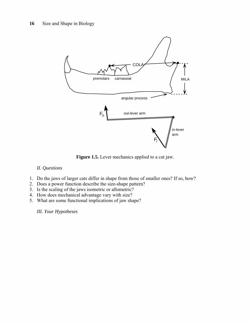
16 Size and Shape in Biology
premolars carnassial
COLA
MILA
angular process
out-lever arm
in-lever arm
Fi
Fo
Figure 1.5. Lever mechanics applied to a cat jaw.
II. Questions
1. Do the jaws of larger cats differ in shape from those of smaller ones? If so, how? 2. Does a power function describe the size-shape pattern? 3. Is the scaling of the jaws isometric or allometric? 4. How does mechanical advantage vary with size? 5. What are some functional implications of jaw shape?
III. Your Hypotheses

Size and Shape in Biology 17
IV. Methods
Measure the MILA and COLA of each jaw with calipers or a ruler: V. Results
1. Plot the log (MILA) on the y-axis against the log (COLA) on the x-axis. 2. Analyze the shape of the curve (is it a fairly straight line, broken line, or curve?) and
calculate the slope (scaling exponent) if appropriate. 3. Calculate mechanical advantage for each jaw. (Hint: Use StatView by creating a new
column in the data set called “MA”, selecting source “dynamic formula”, and entering the formula in the popup menu.)
4. Attach your data table and graphs to your lab report, making sure to label columns and axes
and include units. Include the statistics you calculated and give the power function equation and scaling exponent (both least squares and reduced major axis estimates) for each graph. Use the 95% confidence interval of the scaling exponent to test whether the observed exponent was significantly different from your prediction or from isometry. VI. Conclusion
Write several paragraphs describing your findings, answering the initial questions, and explaining why you accept or reject your hypotheses. Discuss the functional implications for the animal of the relationships you found.
Scaling Exercise 5: The Cat Cranium
I. The Organisms
Domestic cat, clouded leopard, cougar, Siberian tiger, saber tooth cat, American lion: These cats all belong to the Family Felidae, a group specialized as carnivores. The African lion and Siberian tiger are the largest living cats, but other large felids were dominant predators in North America in the past. The skulls you will examine include casts of two extinct species, the saber tooth cat and American lion, recovered from the La Brea tar pits in Los Angeles. The saber tooth cat is noted for its long upper canines (the “sabers”), which are believed to have been useful in stabbing and slicing large thick-skinned herbivores, such as mastodons. One theory about the extinction of large mammals in North America at the end of the Pleistocene attributes the decline of large herbivores like the mastodon to direct hunting by humans, which led to the extinction of large predators such as the saber tooth due to the scarcity of large prey. The focus of this exercise is the scaling of the cranium, the part of the skull that encloses the brain, with body size. The width of the cranium constrains the size of the brain, and can be used as an index of brain size. Other dimensions of the skull will be used as an index of body size in the absence of data on the masses of the animals these skulls came from.

18 Size and Shape in Biology
II. Questions
1. Do the skulls of larger cats differ in shape from those of smaller ones? If so, how? a. How does cranium width vary with skull size? b. Does a power function describe this pattern? c. Is the scaling of the crania isometric or allometric with respect to skull size? 2. Did the extinct sabertooth cat have a brain substantially larger or smaller for its body size
than living cats?
III. Your Hypotheses
IV. Methods
Measure the following dimensions of each skull with calipers or a ruler. Cranium width: - the maximum width of the bulging part of the cranium. Skull width: - the maximum width of the skull. Mandible length: - the maximum length of the lower jaw (mandible).
V. Results
1. On two separate graphs, plot the log (cranium width) on the y-axis against the log (skull width) and log (mandible length) on the x-axes.
2. Analyze the shapes of the curves (are they fairly straight lines, broken lines, or curves?) and
calculate the slopes (scaling exponents) if appropriate. 3. Attach your data table and graphs to your lab report, making sure to label columns and axes
and include units. Include the statistics you calculated and give the power function equation and scaling exponent (both least squares and reduced major axis estimates) for each graph. Use the 95% confidence interval of the scaling exponent to test whether the observed exponent was significantly different from your prediction or from isometry.

Size and Shape in Biology 19
VI. Conclusion
Write several paragraphs describing your findings, answering the initial questions, and explaining why you accept or reject your hypotheses. Discuss the functional implications for the animal of the relationships you found. Scaling Exercise 6: Dog and Wolf Skulls
I. The Organisms
The domestic dog, Canis familiaris, and the wolf, Canis lupus: Dogs are believed to have evolved from some subspecies of the wolf by some combination of natural selection and artificial selection (that is, selection by humans). Skeletal remains of early dogs from archeological sites suggest that their domestication began about 10,000-14,000 years ago (Clutton-Brock and Jewell 1993), but recent phylogenies based on mitochondrial DNA push the dog origin back to more than a million years ago (Cohn 1997, Morell 1997, Vila et al. 1997). In either case, the dog is believed to be the first domesticated animal. Fossils of early dogs show a progressive decrease in body size from the ancestral wolf. The evolution of larger dogs probably occurred long after the initial domestication of the wolf ancestors. Modern dogs differ from wolves not only in appearance, but also in adult behavior and age of reproductive maturity (6–12 months for dogs, 2 years for wolves). Modern dog breeds show a remarkable variety of head shapes, yet the heads of adult wolves are relatively uniform in appearance. How might such a diversity of dog breeds result from an ancestor that showed so little variation in head shape? One mechanism known to generate variation in form is heterochrony, an evolutionary change in the timing of development. (Development here refers to the entire history of an organism from a fertilized egg to maturity.) To determine whether heterochrony might have contributed to the evolution of the dog, you will investigate the changes in head shape that occur in the development of a hypothetical ancestral dog. You will be provided with diagrams of skulls representing a developmental series from fetus to adulthood of a hypothetical ancestral dog, and several skulls (real or plastic casts) of breeds of modern dogs, including pug, Pekinese, and English bulldog. (The plastic casts were made from real skulls in the collection of the Field Museum of Natural History, Chicago, Illinois.)
II. Questions
1. As the ancestral dog grows in size from a fetus to a mature adult, does the overall shape of the skull change? If so, how? a. Does a power function describe the growth pattern? b. Would you consider the growth isometric or allometric?
2. How do the shapes of the adult dog skulls compare with the developmental series of ancestral dog skulls?
3. What role, if any, might heterochrony have played in the evolution of modern dogs from a wolf ancestor?
III. Your Hypotheses

20 Size and Shape in Biology
IV. Methods
1. Measure the following two linear dimensions of each skull in the "ancestral dog" illustrations with a ruler: a. Skull length: the distance from the tip of the snout (excluding the teeth) to the back of the
cranium. b. Cranial width: This is the greatest distance you can find between the right and left sides
of the cranium (brain case). 2. With calipers, measure the same two parameters on the dog skulls.
Skull Length
Cranial Width
Figure 1.6. Dorsal view of a dog skull showing the measurements you will take. V. Results
1. Plot log (skull length) on the y-axis against log (cranial width) on the x-axis. Plot the data for the adult dog skulls on the same graph as the ancestral dog growth series data.
2. Analyze the shape of the curve (is it a fairly straight line, broken line, or curve?) and
calculate the slope (scaling exponent) if appropriate. 3. Analysis hints: If you want to distinguish between dogs and the ancestral dog in your
graphs, create a column for “Species”, go to the Analyze menu and choose Graphs > Bivariate Scattergrams, and place the variable Species in the “Split By” box. If you want to perform regressions on subsets of your data in StatView, highlight the rows you wish to exclude from analysis and select Exclude Row from the Manage menu. Those row numbers will then appear in light gray and their data will disappear from any graphs and analyses you have open.
4. Attach your data table and graphs to your lab report, making sure to label columns and axes
and include units. Include the statistics you calculated and give the power function equation

Size and Shape in Biology 21
and scaling exponent (both least squares and reduced major axis estimates) for each graph. Use the 95% confidence interval of the scaling exponent to test whether the observed exponent was significantly different from your prediction or from isometry. VI. Conclusion
Write several paragraphs describing your findings, answering the initial questions, and explaining why you accept or reject your hypotheses. Discuss the functional implications for the animal of the relationships you found. Scaling Exercise 7: Mammalian Femurs
I. The Organisms
Mouse, rat, chevrotain, cat, peccary, deer, bear, human, horse: The chevrotain, or mouse deer, is a cat-sized animal from the tropics of West Africa and Malaysia. The peccary, common in South America and as far north as Texas, is closely related to pigs. All of these mammals are capable of running gaits in which all feet are off the ground at some point during the stride (called a suspension) and the full weight of the body is placed on the hind legs for at least part of the stride. The femur, or thigh bone, transmits force from the lower leg to the pelvis in running. The strength of a bone depends on its cross-sectional area and the load on a bone depends on the mass of the animal, which is proportional to its volume. If all else is the same, then the stress on a bone can be calculated as
stress = load/cross-sectional area
II. The Questions
1. If femurs scale isometrically, will the strength of the femur be proportional to the load on it as size varies from a mouse to a horse? (Hint: What would a graph of log (stress) vs. log (femur length) look like?)
2. Do the femurs of larger mammals differ in shape from those of smaller ones? If so, how? a. Does a power function describe the relationship between femur length and diameter in
mammals? b. Is the scaling of the femurs isometric or allometric?
3. What are some functional implications of femur shape?
III. Your Hypotheses

22 Size and Shape in Biology
IV. Methods
1. Measure the following two linear dimensions of each specimen with calipers or a ruler: a. Femur diameter: The narrowest part of the femur might be considered the weak link in
transmitting force without breaking. Measure the smallest diameter you can find in the middle of the femur.
b. Femur length: Measure the total length of the femur. This can be taken as a crude measure of the size of the animal. (How well do you think this measure represents body size? What measure would be better?)
2. Plot log (femur diameter) on the y-axis against log (femur length) on the x-axis. 3. Analyze the shape of the curve (is it a fairly straight line, broken line, or curve?) and
calculate the slope (scaling exponent) if appropriate. V. Results
Attach your data table and graphs to your lab report, making sure to label columns and axes and include units. Include the statistics you calculated and give the power function equation and scaling exponent (both least squares and reduced major axis estimates) for each graph. Use the 95% confidence interval of the scaling exponent to test whether the observed exponent was significantly different from your prediction or from isometry.
VI. Conclusion
Write several paragraphs describing your findings, answering the initial questions, and explaining why you accept or reject your hypotheses. Discuss the functional implications for the animal of the relationships you found. Using StatView 4.5 to Analyze Scaling Data
Creating the data set
Each column in your data set will be a variable, such as length, area, or mass, and each row will represent a single individual that you measure (whether a mussel, human, cat skull, etc.). The first step is to specify the variable names and the characteristics of each.
1. Choose StatView 4.5 from the Apple menu. 2. Choose “New” from the “File” menu. You should see a data window split into an upper
“attribute pane”, which describes the columns, or variables, of your data, and a lower pane which will contain your actual data.
3. Click once on the cell called “Input Column” (the whole column will then be highlighted) and type in a name for your first variable (something descriptive like “skull length” or “area”). Notice that a new column has appeared to the right.

Size and Shape in Biology 23
4. Select the appropriate characteristics of your first variable by clicking and holding on each attribute below the title of the column and selecting from the list of choices that appear:
Type: Choose “Real” for continuous numerical variables (such as length or area). Choose “String” for non-numerical variables (such as species).
Source: Choose “User Entered” if you will be typing the values in. Choose “dynamic formula” if you want the values to be calculated automatically from another variable in the data set (more about this later).
Class: The default format should work. “Continuous” is appropriate for continuous numerical values and “Nominal” for string variables.
Format: The default format should work. Dec. Places: Choose the number of decimal places you wish displayed.
5. Enter your observations by clicking on the appropriate cell (shaded if it is a new row). Remember that each row should represent all the measurements you take on a single individual.
6. Save your data set! Calculations
Once you’ve entered your measurements, you can use formulas to create new variables from existing ones. For instance, you might be interested in knowing the area of a series of circles whose diameters you have measured. Create a new column and under the “Source” attribute select “Dynamic Formula.” A formula window will appear and you can type the formula you need into the box called “Formula variable definition.” You can use any of the function buttons under the box as well as other functions listed to the left. To incorporate other variables from your data set (such as “Diameter”), position the cursor in the formula box where you want the variable to appear, then double click on the variable name that appears in the box to the left. If you wanted to calculate the area of a circle given a diameter measurement, the formula should appear in the box as
3.14 * (Diameter/2) ^ 2
and, once you click the “Calculate” button, this column would consist of the areas of all circles whose diameters were entered in the “Diameter” column. Use this approach to calculate the logs of the variables of interest. Remember that the log transformation of a power function (y = a• xb) allows us to estimate the scaling exponent (b) by performing a least squares linear regression. For instance, if your original measurements were shell length and shell mass, you’ll want to create new columns called log (shell length) and log (shell mass) to use in the linear regression.
Regression Analysis and Graphing
1. Once you have created the variables you want to analyze and graph, click on the “Analyze” menu and choose “Regression > Regression - Simple”. In the window that appears, assign one variable as a dependent variable (y-axis) and another variable as an independent variable (x-axis) by clicking and dragging the variable name into the appropriate slot on the left.

24 Size and Shape in Biology
2. Next click “OK” and StatView will open what it calls a “View”, which is a new file showing any analyses and graphs you have done. This file is separate from your data set and should be saved with a different name. When you copy your data to a floppy disk or to a server, be sure to copy both the data file and the view file.
3. The view should now contain three tables of statistics followed by a graph of your data. The least squares regression line is shown and the equation of the line is given below the graph (in the form Y = intercept + slope * X). Remember that it is the slope of this line, the scaling exponent “b”, we are interested in. As mentioned earlier, this estimate of b from the least squares linear regression is biased, and a better estimate can be obtained by dividing the slope by the correlation coefficient, R, which is shown in the Regression Summary table at the top of the View.
4. Suppose you predicted a slope of 2.0 for your graph, and found a slope of 1.8 based on your data. Is your measured slope significantly less than 2.0, or is the deviation due just to random error in the data? One simple way to answer this question is to compute the 95% confidence interval of your slope estimate. To generate this, look in the Analysis Browser window on the left side of the View and click on the triangle next to “Regression” to display a list of optional statistics available with a regression analysis. Highlight “Confidence Intervals”, then click the “Create Analysis” button above. The table of confidence intervals should appear at the bottom of the view. If the predicted value falls within the 95% confidence interval (e.g. the C.I. is 1.55 to 2.05), then the difference between the predicted and observed slope is considered to be not significant. If, on the other hand, your 95% C.I. was 1.71 to 1.89, you could conclude that the slope is significantly less than the predicted value of 2.
5. To perform a second regression on another set of variables, start again with step one above. If you start the second regression while the view window is active, then the new analysis will appear right below the first one in the same view window. If you start the analysis while the data window is active, the new analysis will appear in a new view window in a new file.
6. You can move tables and graphs around (by clicking and dragging) and delete unnecessary ones before printing your View file.
Acknowledgments
Michael LaBarbera contributed to the introduction of the student outline and the tutorial. He also provided useful advice during the development of this lab over the last six years. Steven Vogel suggested the exercise on the scaling of human feet. The exercise on the evolution of skull shape in the dog is adapted from a lab written by Michael Foote. Development of this lab exercise was supported by a grant from the Howard Hughes Medical Institute to the Biological Sciences Collegiate Division of the University of Chicago.
Literature cited
Armstrong, E. 1983. Relative brain size and metabolism in mammals. Science, 220:1302–1304.
Biewener, A. A. 1984. Mammalian terrestrial locomotion and size. BioScience, 39:776–783. Biewener, A. A. 1990. Biomechanics of mammalian terrestrial locomotion. Science,
250:1097–1103.

Size and Shape in Biology 25
Calder, W. A. 1984. Size, function, and life history. Harvard University Press, Cambridge, Massachusetts, 431 pages.
Clutton-Brock, J., and P. Jewell. 1993. Origin and domestication of the dog. Pages 21–31 in Miller’s Anatomy of the Dog, 3rd Edition (H. I. Evans, Editor). W.B. Saunders, Philadelphia.
Cohn, J. 1997. How wild wolves became domestic dogs. BioScience, 47:725–728. Drake, S. (translator) 1974. Galileo Galilei, Two new sciences. University of Wisconsin Press,
Madison, Wisconsin, 323 pages. Goldman, C. A., R. R. Snell, D. B. Brown, and J. J. Thomason. 1990. Principles of allometry.
Pages 43–71 in Tested studies for laboratory teaching, Volume 11 (C. A. Goldman, Editor). Proceedings of the 12th Workshop/Conference of the Association for Laboratory Education
(ABLE), 195 pages. Gould, S. J. 1977. Ontogeny and phylogeny. Harvard University Press, Cambridge, 501 pages. Herring, S. W. 1993. Functional morphology of mammalian mastication. American Zoologist,
33:289–299. Hildebrand, M. 1995. Analysis of vertebrate structure, 4th Edition. John Wiley & Sons, New
York, 657 pages. Jerison, H. J. 1969. Brain evolution and dinosaur brains. American Naturalist, 103:575–588. LaBarbera, M. 1989. Analyzing body size as a factor in ecology and evolution. Annual Review
of Ecology and Systematics, 20:97–117. McGowan, C. 1994. Diatoms to dinosaurs: the size and scale of living things. Island Press,
Washington, D. C., 288 pages. McKinney, M. L. and K. J. McNamara. 1991. Heterochrony: the evolution of ontogeny.
Plenum Press. New York, 437 pages. McMahon, T. A., and J. Y. Bonner. 1983. On size and life. W. H. Freeman &Co., New York,
255 pages. Morell, V. 1997. The origin of dogs: Running with the wolves. Science, 276:1647–1648. Morey, D. F. 1994. The early evolution of the domestic dog. American Scientist, 82:336–347. Peters, R. H. 1983. The ecological implications of body size. Cambridge University Press,
Cambridge, 329 pages. Radinsky, L. B. 1985. Approaches in evolutionary morphology: A search for patterns. Annual
Review of Ecology and Systematics, 16:1–14. Schmidt-Nielsen, K. 1984. Scaling: Why is animal size so important? Cambridge University
Press, Cambridge, 241 pages. Sweet, S. S. 1980. Allometric inference in morphology. American Zoologist, 20:643–652. Trombulak, S. C. 1991. Allometry in biological systems. Pages 49–68 in Tested studies for
laboratory teaching, Volume 12 (C. A. Goldman, Editor). Proceedings of the 12th Workshop/Conference of the Association for Laboratory Education (ABLE), 218 pages.
Turnbull, W. D. 1970. Mammalian masticatory apparatus. Fieldiana: Geology, 18:149–356. Vila, C., P. Savolainen, J. E. Maldonado, I. R. Amorim, J. E. Rice, R. L. Honeycutt, K. A.
Crandall, J. Lundeberg, and R. K. Wayne. 1997. Multiple and ancient origins of the domestic dog. Science, 276:1687–1689
Vogel, S. 1988. Life’s devices: The physical world of animals and plants. Princeton University Press, Princeton, New Jersey, 367 pages.
Weijs, W. A. 1994. Evolutionary approach of masticatory motor patterns in mammals. Pages 281–320 in Biomechanics of feeding in vertebrates. Advances in comparative and environmental physiology, Volume 18, Springer-Verlag, Berlin.

26 Size and Shape in Biology
Appendix A: Pre-Lab Tutorial
(The web version of this tutorial can be viewed at the ABLE web site on the web page for this Proceedings volume.)
Figure 1.7.
I. Introduction
Size, shape, and the relationships of each to function are important topics in organismal biology. Whether you are interested in understanding the significance of a particular morphology or interpreting the factors which may underlie a particular evolutionary trend, it is important that you understand the physical consequences and interdependence of organismal form and size. In this lab you will choose a sample of related biological specimens of different sizes, devise hypotheses about whether the shapes of these specimens vary with size and how that might relate to some biologically relevant function, and then test your hypotheses by measuring the specimens. This web-based preliminary exercise is designed to familiarize you with the main concepts you will need to decide on and test your hypotheses.
Before beginning the tutorial, print out the worksheet, which you should complete and hand in at the beginning of the lab. II. Geometric Similarity
If two objects have the same shape, they are said to be geometrically similar. By definition, the ratio of any two linear dimensions of one object will be same for any geometrically similar object. This is easiest to illustrate with simple geometric shapes:

Size and Shape in Biology 27
Figure 1.8.
For each pair of geometrically similar shapes above, the proportions are identical. That is, the ratio of width to height of the rectangles is 2.0, and the ratio of the height to the hypotenuse of the triangles is 0.6. Notice that all dimensions of one can be calculated by multiplying the dimensions of the other by a constant, in these examples 2 (or 1/2). If you make a geometrically similar rectangle three times as high as the small one above, then its width will be three times as big as well, along with its diagonal measurement and perimeter, i.e. ANY linear dimension will be multiplied by the same factor.
What about other characteristics, such as surface area and volume? Do they show the same relationships as linear measurements? If you double the linear dimensions of an object, do you double its surface area and volume also? Would the ratios of volume to surface area or volume to length remain constant? To answer these questions, imagine that you could build the three cubes illustrated below using sugar cubes 1 cm on a side. The first figure is a single sugar cube, the second consists of 8 sugar cubes, and the third is assembled from 27 sugar cubes.

28 Size and Shape in Biology
Figure 1.9. Fill in the table below (on your answer sheet) with calculations for each of the three cubes:
Table 1.2. Measurements of sugar cubes.
small cube medium cube large cube
length (cm)
surface area (cm2)
volume (cm3)
surface area/volume
surface area/length
volume/length
You can determine the areas and volumes intuitively by counting the exposed faces and imagining the hidden faces. Alternatively, you could use the basic formulas for surface area and volume of a cube:
surface area = 6L2
volume =L3 By now you should be aware that for these cubes, at least, the surface area to volume ratio
decreases as the cube gets larger. Not exactly rocket science, and what might this have to do with organisms? More than you might imagine. Nothing is more basic to life than the exchange of materials, and in virtually all cases in biology this exchange occurs through surfaces. Blood exchanges oxygen and carbon dioxide with the atmosphere through the surface of the lung (the alveoli) and with the tissues of the body through the walls of the capillaries. Nutrients enter your body through the surfaces of the stomach and small intestine; wastes leave the blood through the surfaces of tubules in the kidneys. Anything that enters or leaves a cell must pass through the cell membrane, another two dimensional surface. Such processes will obviously be limited, at least in part, by the available surface area through which exchange may occur. On the other hand, the

Size and Shape in Biology 29
rate at which all of these processes of exchange must occur is dictated by the volume of the cell or tissues that are served. Total demand depends on the biomass that must be supported. The quantitative relationship between surface area and volume is thus of primary biological importance.
The relationships between lengths, areas, and volumes of geometrically similar objects can be predicted rather simply. Areas of an object (such as the surface area or cross sectional area) are proportional to the square of the object's length (L2), while its volume is proportional to the cube of its length (L3). Thus, ratios of lengths, areas, and volumes will be proportional to length raised to some power:
Since Surface Area α L2 and Volume α L3,
SA/V α L2/L3 = 1/L or L-1 For the cubes shown above, the SA/V of each cube is 6 /L. The "6" in this case is a constant that works for cubes; other constants would be used for different shapes, but the 1/L works for any shape.
Simply restated, surface to volume ratios are inversely proportional to size (or length). This geometrical observation has profound biological implications. As Julian Huxley once observed, comparative anatomy is primarily the story of the evolutionary struggle to maintain surface to volume relations. Practice Questions 1. How would you predict the ratio of Surface Area to Length to vary with size?
a. Surface Area/Length α 1/L
b. Surface Area /Length α L2
c. Surface Area /Length α L
d. Surface Area /Length α L1/2 2. How would you predict the ratio of Volume to Length to vary with size?
a. Volume/Length α L
b. Volume/Length α L2
c. Volume/Length α L3 d. Volume/Length α L3/2
III. The Power Function
A way of formalizing these geometric relationships is to use a power function: y = a xb where x and y are the variables you want to relate (such as length or volume), and a and b are parameters that describe the relationship. For example, if you want to relate the volume and radius of a sphere, the power function is Volume =( 4/3 π) radius3 x is radius, y is volume, a takes the value of ( 4/3 π), and b is 3. The table below shows the values of a and b describing various relationships between areas, volume, and linear

30 Size and Shape in Biology
30
dimensions of two common geometrical shapes.
Table 1.3. Values of a and b for two geometric shapes. shape � y� x� b� a� cube � surface area length 2� 6� � cube� volume � length 3� 1� � sphere� surface area� radius� 2� 4π� � sphere� cross section� radius� 2� π� � sphere� volume radius � 3� 4/3 π� � Note that b, the scaling exponent, could be predicted easily by the methods you learned
earlier. The other parameter, a, depends on the shape of the object in question. For most of this discussion, we will ignore the value of "a" merely because it is shape-specific. Note that regardless of shape, volumes (for example) are always proportional to a length cubed, and can be expressed as we did earlier:
V � L3 You can work out other relationships for yourself if you remember the rules for working with exponents. For example, if we let V = volume, A = surface area, and L = length, then:
A � L2 or L � A1/2
V � L3 or L � V1/3
therefore, A � L2 � (V1/3 )2 � V2/3 Power functions can be awkward if you don't already know the value of the exponent. For
example, the graph below plots the volume of a cube versus the length of one side.
Figure 1.10.

Size and Shape in Biology 31
If you didn't already know that the exponent "b" was equal to three, could you deduce it from this plot? Not likely, but here is an easier way. If you plot the same information on log-log graph paper, the relationship appears linear, with the slope equal to the scaling exponent "b."
Figure 1.11.
To make the computation of the slope easier, you can plot log (y) against log (x) as follows:
Figure 1.12.
This is the equivalent of doing a logarithmic transformation of our original equation:

32 Size and Shape in Biology
y = a xb log (y ) = log (a xb)
log (y ) = loga + log (xb)
log (y ) = log a + b log x This last equation describes the straight line on the graph above with slope b and y-intercept of log a.
You can estimate the scaling exponent (b) by doing a least squares linear regression of log y on log x, but the estimate of b (the slope of the line) is somewhat biased. This bias occurs because least squares linear regression techniques assume that all of the errors in your measurements lie in the y variable and that the x variable is known without error. A better technique is reduced major axis regression, which assumes that the errors are evenly partitioned between the x and y variables. Although reduced major axis regression is rarely included in commercial software packages, by a fortunate fluke of the mathematics, the reduced major axis slope is equal to the least squares slope divided by the correlation coefficient (r). In the exercises you'll do in lab, we'll expect you to report both the least squares and reduced major axis estimates of b.
So far we have used simple geometrical shapes to illustrate the relationships between lengths, areas, and volumes because they have simple equations for each of these measures. You have probably noticed that most organisms have complicated shapes that can not be so easily represented mathematically. However, the proportionalities between lengths, areas, and volumes hold for complex shapes as well as simple ones, as long as they are geometrically similar. That is, if we consider a species of snail that exhibits a constant shape regardless of size, then the surface area of its shell will be proportional to its (height)2 , and if you plot log(surface area) vs. log(height), you'll find a straight line with b = 2. IV. Isometric vs. Allometric
Isometry Geometrically similar objects exhibit what is called isometric scaling (iso = same, metric =
measure); the relationships between surface area, volume, and length follow the simple rules we noted earlier. That is, if we consider a species of snail that exhibits a constant shape regardless of size, then the volume enclosed by its shell will be proportional to its (height)3 . To test this, you could collect 100 shells of different sizes, measure the height and volume of each, and plot log(volume) vs. log(height). If scaling is isometric in the shells of this species, then the data should fall along a straight line with slope b = 3.
Allometry
When an animal (or organ or tissue) changes shape in response to size changes (i.e., does not maintain geometric similarity), we say that it scales allometrically (allo = different, metric = measure). Allometric scaling is common in nature, both when comparing two animals of different sizes and when comparing the same animal at two different sizes (i.e., growth). The reasons, and there are many, underlying this rule will keep us occupied for much of this course.

Size and Shape in Biology 33
Using Isometry and Allometry
Example: How do lungs scale with body size in mammals? The primary function of lungs, gas exchange, is accomplished in the alveoli (thin sacks filled with air and lined with blood capillaries). Oxygen diffuses from air into the blood across the lining of the alveoli as carbon dioxide diffuses in the opposite direction. How would you expect the surface area of the alveoli to scale with body mass in a series of mammals from mice to elephants?
Hypothesis 1: Lungs scale isometrically. If large mammals were simply scaled-up versions of small ones (i.e., geometrically similar), then what relationship would we predict between alveolar surface and body mass? If you set y = alveolar surface and x = body mass, the power function is
alveolar surface α (mass)b or
alveolar surface = a (mass)b
The question now becomes what scaling coefficient (b) corresponds to isometry?
Figure 1.13.
To figure this out, convert each variable into a length raised to some power. Alveolar surface
is an area, and for isometric scaling, area α L2 .
Body mass is proportional to volume (as most animals have similar densities), and
volume α L3
The predicted scaling coefficient for isometry can be calculated as the exponent on the y-axis divided by the exponent on the x-axis, so in this case b = 2/3 or 0.67.

34 Size and Shape in Biology
Figure 1.14.
Hypothesis 2: Lungs scale allometrically. Any scaling coefficient other than 2/3 would indicate an allometric relationship between lung size and body mass, but you might consider what coefficient is appropriate to the function of the lungs. If the tissues of large animals have the same need for gas exchange surface as those of small animals, then alveolar surface area should be proportional to body mass, or
alveolar surface α (mass)1
which would mean a scaling exponent of 1.
Testing your hypotheses: If you actually measure body mass and alveolar surface area for a variety of mammals and perform a linear regression of log(alveolar surface) against log(mass), the slope is about 1.02–1.06. Thus scaling of mammalian alveoli is allometric, and the specific hypothesis that alveolar surface is proportional to body mass is supported. Elephants have more alveolar surface than would be the case if their lungs were scaled up isometrically from those of mice. If the slope had turned out to be 0.4, then we would still have rejected the hypothesis of isometry and accepted the hypothesis of allometry, but not the specific form of allometry we had predicted.
Figure 1.15. Structural Support: Structures break when the load (force) per unit cross sectional area exceeds the strength of the material from which the structure is built. A tree trunk, for instance, must be strong enough to support the tree's branches and leaves against the force of gravity and to

Size and Shape in Biology 35
withstand the forces exerted by winds, but must not be so large that it crushes under its own weight. Similarly, the limbs of terrestrial animals, whether they be elephants or insects, must support the weight of the animal's body without being so large that moving the legs during locomotion becomes too costly. Within most groups of organisms, density is relatively constant, so the load on the support structure is proportional to the volume of the organism. The strength of the support material is generally proportional to its cross-sectional area (e.g. the area of wood exposed when you cut through a tree trunk). Think about the implications of this for support of large organisms. Will isometrically scaling organisms be relatively robust or fragile as they get bigger? Practice Questions (click answer to test your response) For each example, pick the scaling exponent, b, that would signify an isometric relationship . Assume that the log of the first variable would be plotted on the y-axis and the log of the second variable on the x-axis. 1. Trunk diameter vs. height in oak trees.
b = 0.33 b = 0.5 b = 1.0 b = 2.0 2. Trunk cross-sectional area vs. total above-ground mass in oak trees.
b = 0.33 b = 0.67 b = 1.0 b = 1.5 3. Total leaf area vs. height in oak trees.
b = 0.5 b = 1.0 b = 2.0 b = 3.0 Worksheet Questions
Question 2 on the worksheet asks that you calculate the dimensions of a sugar cube that would crush under its own weight, given its density, its crushing strength (which is equivalent to about 200 lb. for an average sugar cube - if you don't believe this, try standing on one!), and the acceleration due to gravity. Hint: What you need to figure out is the length of one side of a cube whose weight (mass times acceleration due to gravity) divided by the area of the bottom face is equal to the crushing strength. The answer will surprise you. The point is that there are limits to size for anything - sugar cubes, mountains, or organisms.
For question 3 on the worksheet, use the discussion of scaling of mammalian alveoli above as an example of how to tackle the four cases in the question. It's helpful to think of the graphs you would make and the power function appropriate for that case.
The scaling principles we've presented can be used with certain other properties of organisms besides the three spatial dimensions, for instance heartbeat frequency or metabolic rate. After completing question 5 on the worksheet, examine the following statistics and contemplate the significance of scaling of metabolic rate with body size for thermoregulation for large animals:
Table 1.4. Metabolic rates of camels and mice.

36 Size and Shape in Biology
heat output of a resting 409 kg. camel 240 watts
heat output of a resting 20g mouse 0.2 watts
heat output of 409 kg of resting mice 3840 watts
Worksheet for Size and Shape in Biology Tutorial Scaling of cubes: fill in the table
Table 1.5. Measurements of sugar cubes.
small cube medium cube large cube
length (cm)
surface area (cm2)
volume (cm3)
surface area/volume
surface area/length
volume/length
1. How big could a sugar cube get before the bottom crushed under its own weight?
useful info: density = 1040 kg/m3
crushing strength = 5.17x10⁶ Newtons/m2
acceleration due to gravity = 9.81 m/second2
2. For each of the four examples below, the slope of a power function is given which compares two measurements of a group of organisms. For each, give the slope you would expect if the relationship is isometric, and state whether the observed relationship is isometric or allometric. The log of the first variable would be plotted on the y-axis and the log of the second on the x-axis.
a. Arm length vs. body height for infant humans: b=1.2 b. Brain mass vs. body mass in humans: b=0.66 c. Mass of skeleton vs. body length in whales: b=3.07 d. Mass of skeleton vs. body length in terrestrial mammals: b=3.25
3. Dr. Colton's house (10m wide, 20m long, 4m high - just a hovel, really) has a 30,000 watt furnace that just barely keeps him warm on cold Chicago nights. He's thinking of building a larger house to accommodate his growing collection of abalone shells, and needs advice on the output of the new furnace. The new house will be 3 times as high, 3 times as wide, and 3 times as long.

Size and Shape in Biology 37
a. If he assumes that the furnace size should be proportional to the volume of the house, then what size furnace should he install?
b. If heat loss depends on the surface area of exterior walls, roof, and floor exposed to the winter cold rather than on the volume of the house, then what size furnace would you recommend?
4. Mammals are endothermic, maintaining fairly constant high body temperature by their metabolism. Metabolic rate is a measure of the heat production (and thus heat loss) of an organism.
a. If resting metabolic rate is proportional to the mass of tissue in an animal, then what would be the slope of a graph of log(resting metabolic rate) vs. log(mass)?
b. Some studies have found this slope (within one species) to be 2/3. Propose a hypothesis to account for this based on the principles explored in the home furnace question.
c. Given the observed relationship between metabolic rate and size, what differences might you find in equivalent-sized cells from a mouse and an elephant?
Appendix B: Notes and Expected Results for Each Exercise
Exercise 1: Mussel Shells
Mussel shells can be collected to span a 10-fold range of lengths, which corresponds to a more than 1000-fold range of masses. Students choose which linear dimensions to measure in addition to mass. They usually measure “length” as the maximum distance along the antero-posterior axis (longest shell dimension) and “width” as the distance along either the dorso-ventral axis or the right-left axis. If shells are isometric, then length α (width)1 and mass α (length)3. Plausible hypotheses for allometric growth include:
• Shells grow relatively longer in the antero-posterior axis because of competition from other mussels on the rock. (A closeup picture of a dense mussel bed helps students understand the geometry of growth relative to the substrate and neighbors.) Thus b > 1 for length α (width)b.
• Shells grow relatively thicker to resist predation from birds (who drop shell from a height to break) and crabs or to resist damage from wave action. This would mean b > 3 for mass α (length)b.
• Shells grow less in thickness because shell strength is not critical to the primary functions of resisting dessication and protecting from starfish (who pry the shell open rather than breaking it). Increases in length and width provide more interior volume for guts and gonads, which are more important for fitness than is shell strength. Thus b < 3 for mass α (length)b.
The set of shells I collected on Campobello Island, New Brunswick, are close to isometric in overall shape, but show positive allometry of shell mass with length (b=3.5). Students sometimes find a slight positive allometry of length with width. The regression statistics provided by StatView 4.5 for shell mass and length data are provided (Fig. 16) as an example of the analysis. The least squares estimate of the scaling exponent, 3.455, is virtually the same as the reduced major axis estimate (3.462) because of the high correlation coefficient (R). The

38 Size and Shape in Biology
relationship is considered allometric because the 95% confidence interval of the scaling exponent does not include the isometric prediction of 3.0.
100
.998
.996
.995
.087
CountNum. Missing
R
R Squared
Adjusted R SquaredRMS Residual
Regression Summary Log Mass vs. Log Length
-5.257 .123 -5.257 -42.893 <.0001
3.455 .080 .998 43.123 <.0001
Coefficient Std. Error Std. Coeff. t-Value P-Value
Intercept
Log Length
Regression Coefficients Log Mass vs. Log Length
-5.257 -5.540 -4.975
3.455 3.270 3.639
Coefficient 95% Lower 95% Upper
Intercept
Log Length
Confidence Intervals Log Mass vs. Log Length
-2.5
-1.5
-0.5
0.5
1.5
Log
Mas
s
.8 1 1.2 1.4 1.6 1.8 2
Log Length
Y = -5.257 + 3.455 * X; R^2 = .996
Regression Plot
Figure 1.16. Mussel shell mass vs. shell length. Graph and tables of regression statistics
from StatView 4.5 software. Exercise 2: Stress and the Human Foot
If the video camera and AV-capable computer for measuring foot area are not available, area could be measured by cutting out the tracings and weighing them on a toploading balance. Alternatively, students could measure the length and width of the feet with calipers and examine how mass varies with foot length, width, and length x width. It is critical to get a broader range of body sizes than is available in a typical college class. To extend the range, we provide foot tracings with annotated weights for several children. Plausible hypotheses about the scaling of mass and foot area include:
• Foot area scales isometrically with body size, with b = 0.67 for Area α (Mass)b. This would result in higher stresses on the feet of larger people.
• Foot area shows positive allometry with body mass so that stress on the foot does not change with size. Since area would be directly proportional to mass, we would expect b = 1.
The data we have collected so far show foot area to be isometric or negatively allometric with body mass (0.5 < b < 0.7). This means that stress increases substantially with body size (Fig. 17). All of our labs have used the same small set of children’s foot tracings, which strongly affect the estimate, so this result may not be general. A class at Duke University performing a similar exercise found stress to be constant over a wide range of body sizes, but they used height rather than mass as their measure of body size (Steven Vogel, personal communication).

Size and Shape in Biology 39
1.9
2.1
2.3
2.5
log
(Are
a)
1.0 1.2 1.4 1.6 1.8 2.0 2.2log (Mass)
Y = 1.342 + .515 * X; R^2 = .931
Scaling of Foot Area with Mass
0
1
2
3
4
5
Stre
ss (N
/cm
2)
0 20 40 60 80 100 120 140Mass (kg)
Y = 1.39 + .029 * X; R^2 = .876
Stress vs. Body Mass
Figure 1.17. Scaling of the human foot with body mass. Left, log of foot area vs. log of body mass. Right, log of stress on foot vs. body mass.
Exercises 3 and 4: Jaws of Ruminants and Cats
This exercise uses a static analysis of chewing force, sensu the vertical "jaw closing force" of Turnbull (1970). It ignores the role of transverse movements of the mandible, which are particularly important in ungulates (Weijs 1994). The concept of lever mechanics used here can be problematic for students with weak physics backgrounds. In-lever lengths and out-lever lengths can be demonstrated using a nutcracker as a prop. If students understand that moving the nut closer to the hinge or their hands further from the hinge increases the crushing force, then they have an intuitive grasp of the physics involved. The MILA we measure is a rough approximation of the in-lever arm of the superficial masseter, which actually inserts on a broad area of the mandible. The mechanical advantage calculated as MILA/COLA represents the multiplier of the force generated by the masseter as it is translated by the jaw to a chewing force If scaling is isometric, then the mechanical advantage should be the same for all species. A positive allometry for MILA or a negative allometry for COLA would correspond to a higher mechanical advantage for large species, resulting in a relatively greater chewing force. An increase in mechanical advantage is not the only way of increasing force, however. Chewing force is influenced by the cross-sectional area of the masseter, as well as the angle of its force vector with the lever arm, sarcomere stretch, and velocity of contraction (Herring 1993), but these are difficult to estimate from skeletons. In addition, other muscles, such as the temporalis and pterygoid, are involved. Conclusions from this exercise are limited to the role of mechanical advantage in force generation by the masseter. Plausible hypotheses about jaw scaling include:
• Scaling is isometric because the feeding mode within each group does not vary much with size. Thus b=1 for MILA α (COLA)b.
• MILA shows positive allometry with respect to COLA, meaning higher mechanical advantages in larger animals. This would tend to increase the chewing force in larger
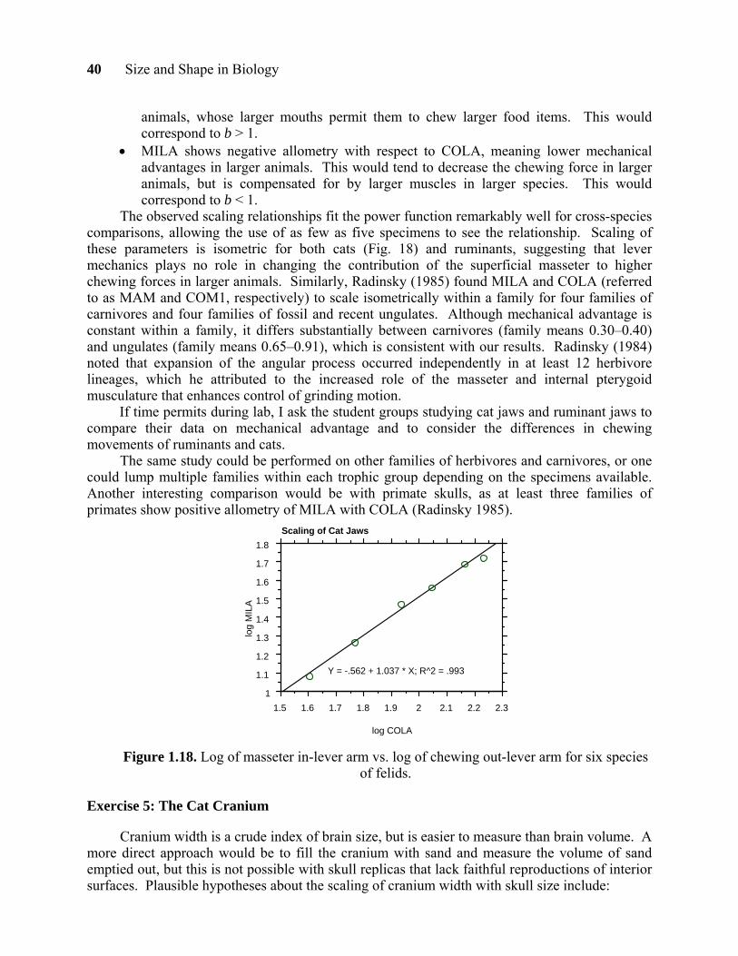
40 Size and Shape in Biology
animals, whose larger mouths permit them to chew larger food items. This would correspond to b > 1.
• MILA shows negative allometry with respect to COLA, meaning lower mechanical advantages in larger animals. This would tend to decrease the chewing force in larger animals, but is compensated for by larger muscles in larger species. This would correspond to b < 1.
The observed scaling relationships fit the power function remarkably well for cross-species comparisons, allowing the use of as few as five specimens to see the relationship. Scaling of these parameters is isometric for both cats (Fig. 18) and ruminants, suggesting that lever mechanics plays no role in changing the contribution of the superficial masseter to higher chewing forces in larger animals. Similarly, Radinsky (1985) found MILA and COLA (referred to as MAM and COM1, respectively) to scale isometrically within a family for four families of carnivores and four families of fossil and recent ungulates. Although mechanical advantage is constant within a family, it differs substantially between carnivores (family means 0.30–0.40) and ungulates (family means 0.65–0.91), which is consistent with our results. Radinsky (1984) noted that expansion of the angular process occurred independently in at least 12 herbivore lineages, which he attributed to the increased role of the masseter and internal pterygoid musculature that enhances control of grinding motion.
If time permits during lab, I ask the student groups studying cat jaws and ruminant jaws to compare their data on mechanical advantage and to consider the differences in chewing movements of ruminants and cats. The same study could be performed on other families of herbivores and carnivores, or one could lump multiple families within each trophic group depending on the specimens available. Another interesting comparison would be with primate skulls, as at least three families of primates show positive allometry of MILA with COLA (Radinsky 1985).
1
1.1
1.2
1.3
1.4
1.5
1.6
1.7
1.8
log
MIL
A
1.5 1.6 1.7 1.8 1.9 2 2.1 2.2 2.3
log COLA
Y = -.562 + 1.037 * X; R^2 = .993
Scaling of Cat Jaws
Figure 1.18. Log of masseter in-lever arm vs. log of chewing out-lever arm for six species
of felids. Exercise 5: The Cat Cranium
Cranium width is a crude index of brain size, but is easier to measure than brain volume. A more direct approach would be to fill the cranium with sand and measure the volume of sand emptied out, but this is not possible with skull replicas that lack faithful reproductions of interior surfaces. Plausible hypotheses about the scaling of cranium width with skull size include:

Size and Shape in Biology 41
• Scaling is isometric, with b = 1 for Cranium width α (Skull width or Mandible length) b. This would be consistent with brain size being proportional to body size. One rationale would be that a larger body needs neural coordination in proportion to its volume, so the brain should be a constant fraction of body mass.
• Cranium width is negatively allometric with skull size, with b < 1 for Cranium width α (Skull width or Mandible length) b. This would suggest that brain size is a smaller fraction of body mass in larger animals. One rationale would be that sensory information that must be integrated by the brain is proportional to surface area (which increases with the 2/3 power of volume) and that the number of muscles that must be controlled may not vary much with size within the felids, so larger species should not need as proportionately large a brain.
For my sample of six species of felids, b = 0.58–0.60 comparing cranium width to a variety of linear skull size measures (Fig. 19). Early studies of the scaling of mammalian brain mass with body mass found an exponent of 0.67, but more recent studies including larger numbers of species support an exponent of 0.75 (Radinsky 1985, Vogel 1988). This discrepancy may by due to the inclusion of more small mammals in the larger datasets (Radinsky 1985). This might explain the low exponent that I find in the felids, which lack small-bodied species. One hypothesis proposed to explain the negative allometry of brain size with body size is that brain size is proportional to basal metabolic rate, which is proportional to (body mass)0.75(Armstrong 1983). Other groups of vertebrates show the same scaling exponents of brain size to body mass as mammals, but differ in the y-intercept (equivalent to log a) (Hildebrand 1995). One application of brain scaling is debunking popular beliefs that certain large-bodied species had unusually small brains. Dinosaurs, for instance, were considered to have unusually small brains, when in reality their brain sizes fit the general pattern for reptiles, amphibians, and fishes (Jerison 1969). Similarly, my data are consistent with the hypothesis that the extinct saber tooth cat and American lion had brain sizes in the normal range for felids.
1.6
1.7
1.8
1.9
2.0
2.1
log
(Cra
nium
Wid
th)
1.8 2.0 2.2 2.4
log (Skull Width)
Y = .57 + .584 * X; R^2 = .974
Scaling of Cranium with Skull Width
1.6
1.7
1.8
1.9
2.0
2.1
log
(Cra
nium
Wid
th)
1.7 1.9 2.1 2.3 2.5
log (Mandible Length)
Y = .576 + .589 * X; R^2 = .966
Scaling of Cranium with Mandible Length
Figure 1.19. Log of cranium width vs. log of skull width (left) or log of mandible length
(right) for six species of felids.

42 Size and Shape in Biology
Exercise 6: Dog and Wolf Skulls
For the growth series of the hypothetical dog ancestor we use a set of approximately life-size drawings of skulls of a great dane. A preferable alternative would be diagrams representing the growth series of a wolf, but I am unaware of any published illustrations. The two measurements were chosen to illustrate the relative increase in snout length in the early development of the dog. One implication of snout elongation is increase in gape size, with presumed advantages in predation and defense. Plausible hypotheses about the scaling of cranium width with skull size include:
• Scaling is isometric, with b = 1 for Skull length α (Cranium width)b. This implies that snout length and gape are proportionately the same at all stages of development. On the graph, the adult dog skulls would then fall far from the ancestral ontogenetic curve because the dog skull shapes clearly differ from the diagram of the adult ancestral dog.
• Scaling is allometric, with b > 1, at least in the later stages of development of the ancestral dog. This would correspond to an elongation of the snout during development. The casts of the adult pug, Pekinese, and bulldog resemble juvenile stages of the ancestral dog. One evolutionary mechanism that might generate the variety of head shapes observed in dog breeds is by stopping development at an earlier stage, so that the head shape of the mature dog resembles that of a juvenile of the ancestral species.
Only the ancestral dog ontogenetic series is used to determine the scaling relationship; the measurements of different breeds of adult dog skulls are plotted for comparison. In contrast to the other six scaling exercises, the power function fails to describe these data adequately. The approach that I use instead is to fit the power function to two subsets of the ancestral dog series, the first three stages and the last four stages (Fig. 20). The exponent for the first stages of development, 1.3, is not significantly different from 1.0, suggesting isometric growth. The exponent for the later stages, 4.5, is significantly greater than 1.0, indicating positive allometry of skull length. The points representing the adult pug, Pekinese, English bulldog, and unknown dog skulls fall close to the fitted regression line for the later stages of development of the ancestral dog, which is consistent with student observations that the adult dog skulls resemble the intermediate developmental stages. This suggests the possibility of heterochrony as a simple mechanism for generating the diversity of head shapes among breeds of dogs. According to the current nomenclature of heterochrony (McKinney and McNamara 1991), this type of paedomorphosis would be considered progenesis, since dogs cease growth and reach sexual maturity at an earlier age than wolves. This paedomorphic reduction in snout length could be due to (1) a reduced need for a wide gape for prey capture and defense, (2) artificial section by humans for a less-threatening, more anthropomorphic head shape, or (3) selection for small body size and early age of reproduction. For a fuller discussion of these issues and the morphological and behavioral evidence for paedomorphosis, see Morey (1994).

Size and Shape in Biology 43
1.4
1.6
1.8
2
2.2
2.4
log
(Len
gth)
1.2 1.4 1.6 1.8log (Width)
dog
ancestral dog
Scaling of skull length with skull width
b = 4.5 R^2 = .943
b = 1.3 R^2 = .998
Figure 1.20. Log of skull length vs. log of cranial width for a hypothetical ancestral dog growth series (circles) and adult dogs of four other breeds (squares). Regression lines were fitted to subsets of the ancestral dog growth series only.
Exercise 7: Mammalian Femurs
The choice of species for this exercise was based on local availability, but other species should work equally well, as the isometric pattern holds fairly generally for mammals smaller than 100 kg in size (Biewener 1990). If the load on the femur is proportional to body mass or volume and the strength of the femur is proportional to its cross-sectional area, then isometric scaling of femurs would result in higher stresses on the femurs of larger animals. One way to understand this is to see that load is a length3 term and strength is a length2 term, so load increases faster than strength as animal size increases. If the diameter increased allometrically to keep stress constant, then diameter would have to increase in proportion to length1.5, making femurs of larger animals proportionately thicker. Plausible hypotheses include:
• Scaling is isometric, with b = 1 for femur diameter α (femur length)b. Stresses would be larger on the femurs of larger animals, all else being equal. Larger animals might suffer greater frequency of injuries or modify their behavior to reduce stresses.
• Femur diameter scales allometrically with length, specifically with b=1.5, which would keep stresses the same for animals of all sizes. Larger animals would have relatively thicker femurs.
The observed scaling exponent of 0.94 in my sample is not significantly different from 1.0, indicating isometric scaling (Fig. 21). This would seem to suggest that the femurs of larger animals should experience higher stresses. However, force plate studies and in vivo measurements of strains in femurs indicate that peak stresses on the limb bones of mammals engaged in strenuous activity are uniform over a body size range of 0.04–300 kg (Biewener 1984). Within this size range, a progressively more upright posture allows larger animals to keep peak stresses constant. An upright limb posture increases the mechanical advantage of the muscles, thereby decreasing the total force applied to the limb bones. At the upper end of this size range (about the size of a horse), animals have a posture that is essentially fully upright, so this strategy cannot explain uniform stresses seen in even larger species. Mammals larger than 300 kg are believed to control stresses by a combination of allometric increases in bone diameter and decreased locomotor performance (Biewener 1990).

44 Size and Shape in Biology
0.0
.4
.8
1.2
1.6
log
(fem
ur d
iam
eter
)
1.0 1.4 1.8 2.2 2.6log (femur length)
Y = -.95 + .939 * X R^2 = .962
Scaling of mammalian femurs
Figure 1.21. Log of femur diameter vs. log of femur length for 11 species of mammals ranging in size from a mouse to a horse.
When the group studying mammalian femurs has finished collecting and analyzing data, I provide them with casts of femurs of two dinosaurs, Tyrannosaurus rex and Triceratops, and ask them to measure the length of each femur, then calculate the diameter they would expect based on the mammalian femur scaling relationship. The observed diameter turns out to be nearly double what they predict, suggesting an allometric scaling of femurs in larger terrestrial vertebrates. If these dinosaur femurs did scale isometrically with smaller mammals, it would suggest that dinosaurs had very limited abilities to engage in strenuous activities such as running or jumping. When presented to the class at the end of the period, this application of scaling to understanding extinct charismatic megafauna serves as a striking coda to the lab.