solved with comsol multiphysics 4.3a heat … with comsol multiphysics 4.3a ... heat transfer...

Solved with COMSOL Multiphysics 4.3a

© 2 0 1 2 C O

Hea t Gen e r a t i o n i n a D i s c B r a k e

Introduction

This example models the heat generation and dissipation in a disc brake of an ordinary car during panic braking and the following release period. As the brakes slow the car, they transform kinetic energy into thermal energy, resulting in intense heating of the brake discs. If the discs overheat, the brake pads stop working and, in a worst-case scenario, can melt. Braking power starts to fade already at temperatures above 600 K.

In the model, the car (1800 kg) initially travels at 25 m/s (90 km/h) when the driver brakes hard for 2 s, causing the vehicle’s eight brake pads to slow the car down at a rate of 10 m/s2. The wheels are assumed not to skid against the road surface. After this period of time, the driver releases the brake and the car travels at 5 m/s for an additional 8 s without any braking. The questions to analyze with the model are:

• How hot do the brake discs and pads become during the braking stage?

• How much do they cool down during the subsequent rest?

Model Definition

Model the brake disc as a 3D solid with shape and dimensions as in Figure 1. The disc has a radius of 0.14 m and a thickness of 0.013 m.

Figure 1: Model geometry, including disc and pad.

M S O L 1 | H E A T G E N E R A T I O N I N A D I S C B R A K E


2 | H E A

Neglecting drag and other losses outside the brakes, the brakes’ retardation power is given by the negative of the time derivative of the car’s kinetic energy:

Here m is the car’s mass, v denotes its speed, R equals the wheel radius (0.25 m), ω is the angular velocity, and α is the angular acceleration. The acceleration is constant in this case, so ω(t) = ω0 + αt.

By definition, the retardation power equals the negative of the work per unit time done by the friction forces on the discs at the interfaces between the pads and the discs for the eight brakes. You can calculate this work as eight times an integral over the contact surface of a single brake pad. The friction force per unit area, ff, is approximately constant over the surface and is directed opposite the disc velocity vector, vd vdeϕ= , where eϕ denotes a unit vector in the azimuthal (angular) direction and the magnitude of vd at the distance r from the center equals vd( r, t ) = ω(t) r. Thus, writing fd ffeϕ= gives the following result for the retardation power:

You can approximate the last integral with the pad’s area, A (0.0035 m2), multiplied by the distance from the center of the disc to the pad’s center of mass, rm (0.1143 m).

Combining the two expressions for P gives the following result for the magnitude of the friction force, ff:

(Note that α is negative during retardation.)

Under the previously stated idealization that retardation is due entirely to friction in the brakes, the heat power generated per unit contact area at time t and the distance r from the center becomes

The disc and pad dissipate the heat produced at the boundary between the brake pad and the disc by convection and radiation. This example models the rotation as convection in the disc. The local disc velocity vector is

Ptd

d mv2

2----------- – m– v vd

td------ m– R2ω t( )α= = =

P 8– ff Ad vd⋅ 8 ff t( ) ω t( ) r Ad= =

ffmR2α8rmA-----------------–=

q r t,( ) f– f vd r t,( )⋅ mR2α8rmA----------------- r ω0 αt+( )–= =

T G E N E R A T I O N I N A D I S C B R A K E © 2 0 1 2 C O M S O L


© 2 0 1 2 C O

The model also includes heat conduction in the disc and the pad through the transient heat transfer equation

where k represents the thermal conductivity (W/(m·K)), Cp is the specific heat capacity (J/(kg·K)), and Q is the heating power per unit volume (W/m3), which in this case is set to zero.

At the boundary between the disc and the pad, the brake produces heat according to the expression for q given earlier. The heat dissipation from the disc and pad surfaces to the surrounding air is described by both convection and radiation

In this equation, h equals the convective film coefficient (W/(m2·K)), ε is the material’s emissivity, and σ is the Stefan-Boltzmann constant (5.67·10−8 W/(m2·K4)).

To calculate the convective film coefficient as a function of the vehicle speed, v, use the following formula (Ref. 1):

Here l is the disc’s diameter. The material properties—the thermal conductivity, k, the density, ρ, the viscosity, μ, and the specific heat capacity, Cp—are those for air.

Table 1 summarizes the thermal properties, which come from (Ref. 1). You calculate the density of air at a reference temperature of 300 K using the ideal gas law.

PROPERTY DISC PAD AIR

ρ (kg/m3) 7870 2000 1.170

Cp (J/(kg·K)) 449 935 1100

k (W/(m·K)) 82 8.7 0.026

ε 0.28 0.8 -

μ (Pa·s) - - 1.8·10-5

TABLE 1: MATERIAL PROPERTIES

vd ω t( ) y– x( , )=

ρ CpT∂t∂------- ∇+ k∇T–( )⋅ Q ρ CP u ∇T⋅–=

qdiss h– T Tref–( ) εσ T4 Tref4

–( )–=

h 0.037kl

------------------Re0.8 Pr0.33 0.037kl

------------------ ρ l vμ---------- 0.8 Cp μ

k-----------

0.33= =



4 | H E A

Results and Discussion

The surface temperatures of the disc and the pad vary with both time and position. At the contact surface between the pad and the disc the temperature increases when the brake is engaged and then decreases again as the brake is released. You can best see these results in COMSOL Multiphysics by generating an animation. Figure 2 displays the surface temperatures just before the end of the braking. A “hot spot” is visible at the contact between the brake pad and disc, just at the pad’s edge—this is where the temperature could become critical during braking. The figure also shows the temperature decreasing along the rotational trace after the pad. During the rest, the temperature becomes significantly lower and more uniform in the disc and the pad.

Figure 2: Surface temperature of the brake disc and pad just before releasing the brake (t = 1.8 s).

To investigate the position of the hot spot and the time of the temperature maximum, it is helpful to plot temperature versus time along the line from the center to the pad’s edge depicted in Figure 3. The result is displayed in Figure 4. You can see that the maximum temperature is approximately 415 K. The hot spot is positioned close to the radially outer edge of the pad. The highest temperature occurs approximately 1 s after engaging the brake.



© 2 0 1 2 C O

Figure 3: The radial line probed in the temperature vs. time plot in Figure 4.

Figure 4: Temperature profile along the line indicated in Figure 3 at the disc surface (z = 0.013 m) as a function of time.

r (m)t



6 | H E A

To investigate how much of the generated heat is dissipated to the air, study the surface integrals of the produced heat and the dissipated heat. These integrals give the total heat flux (J/s) for heat production, Qprod, and heat dissipation, Qdiss, as functions of time for the brake disc. The time integrals of these two quantities, Wprod and Wdiss, give the total heat (J) produced and dissipated, respectively, in the brake disc. Figure 5 shows a plot of the total produced heat and dissipated heat versus time. You can see that 8 s after disengagement the brake has dissipated only a fraction of the produced heat. The plot indicates that the resting time must be extended significantly to dissipate all the generated heat.

Figure 5: Comparison of total heat produced (solid line) and dissipated (dashed).

The results of this model can help engineers investigate how much abuse, in terms of specific braking sequences, a certain brake-disc design can tolerate before overheating. It is also possible to vary the parameters affecting the heat dissipation and investigate their influence.

Reference

1. J.M. Coulson and J.F. Richardson, Chemical Engineering, vol. 1, eq. 9.88; material properties from appendix A2.



© 2 0 1 2 C O

Model Library path: Heat_Transfer_Module/Tutorial_Models/brake_disc

Modeling Instructions

M O D E L W I Z A R D

1 Go to the Model Wizard window.

2 Click Next.

3 In the Add physics tree, select Heat Transfer>Heat Transfer in Solids (ht).

4 Click Next.

5 Find the Studies subsection. In the tree, select Preset Studies>Time Dependent.

6 Click Finish.

G L O B A L D E F I N I T I O N S

Parameters1 In the Model Builder window, right-click Global Definitions and choose Parameters.

Define the global parameters by loading the corresponding text file provided.

2 In the Parameters settings window, locate the Parameters section.

3 Click Load from File.

4 Browse to the model’s Model Library folder and double-click the file brake_disc_parameters.txt.

G E O M E T R Y 1

Cylinder 11 In the Model Builder window, under Model 1 right-click Geometry 1 and choose

Cylinder.

2 In the Cylinder settings window, locate the Size and Shape section.

3 In the Radius edit field, type 0.14.

4 In the Height edit field, type 0.013.

5 Click the Build Selected button.

Cylinder 21 In the Model Builder window, right-click Geometry 1 and choose Cylinder.



8 | H E A

2 In the Cylinder settings window, locate the Size and Shape section.

3 In the Radius edit field, type 0.08.

4 In the Height edit field, type 0.01.

5 Locate the Position section. In the z edit field, type 0.013.


Work Plane 11 Right-click Geometry 1 and choose Work Plane.

2 In the Work Plane settings window, locate the Work Plane section.

3 In the z-coordinate edit field, type 0.013.

4 Click the Show Work Plane button.

Bézier Polygon 11 In the Model Builder window, under Model 1>Geometry 1>Work Plane 1 right-click

Plane Geometry and choose Bézier Polygon.

2 In the Bézier Polygon settings window, locate the Polygon Segments section.

3 Find the Added segments subsection. Click the Add Cubic button.

4 Find the Control points subsection. In row 1, set yw to 0.135.

5 In row 2, set xw to 0.02.

6 In row 2, set yw to 0.135.






12 Find the Control points subsection. In row 2, set xw to 0.03.




16 In row 4, set xw to 0.



19 Find the Control points subsection. In row 2, set xw to -0.035.



© 2 0 1 2 C O


21 In row 3, set xw to -0.03.





26 Find the Control points subsection. In row 2, set xw to -0.05.




30 Click the Close Curve button.

To complete the pad cross section, you must make the top-left and top-right corners sharper. Do so by changing the weights of the Bézier curves.

31 Find the Added segments subsection. In the Added segments list, select Segment 1

(cubic).

32 Find the Weights subsection. In the 3 edit field, type 2.5.

33 Find the Added segments subsection. In the Added segments list, select Segment 4

(cubic).

34 Find the Weights subsection. In the 2 edit field, type 2.5.


Extrude 11 In the Model Builder window, under Model 1>Geometry 1 right-click Work Plane 1 and

choose Extrude.

2 In the Extrude settings window, locate the Distances from Plane section.

3 In the table, enter the following settings:


The model geometry is now complete.

Next, define some selections of certain boundaries. You will use them when defining the settings for model couplings, boundary conditions, and so on.

Distances (m)

0.0065



10 | H E

D E F I N I T I O N S

Explicit 11 In the Model Builder window, under Model 1 right-click Definitions and choose

Selections>Explicit.

2 Right-click Explicit 1 and choose Rename.

3 Go to the Rename Explicit dialog box and type Disc faces in the New name edit field.

4 Click OK.

5 In the Explicit settings window, locate the Input Entities section.

6 From the Geometric entity level list, choose Boundary.

7 Select Boundaries 1, 2, 4–6, 8, 13–15, and 18 only.

Explicit 21 In the Model Builder window, right-click Definitions and choose Selections>Explicit.


3 Go to the Rename Explicit dialog box and type Pad faces in the New name edit field.

4 Click OK.



7 Select Boundaries 9, 10, 12, 16, and 17 only.

Explicit 31 In the Model Builder window, right-click Definitions and choose Selections>Explicit.


3 Go to the Rename Explicit dialog box and type Contact surface in the New name edit field.

4 Click OK.



To select the contact surface boundary, it is convenient to temporarily switch to wireframe rendering.

7 Click the Wireframe Rendering button on the Graphics toolbar.

A T G E N E R A T I O N I N A D I S C B R A K E © 2 0 1 2 C O M S O L


© 2 0 1 2 C O

8 Select Boundary 11 only.

To select this boundary, you typically need to click twice before right-clicking; the first click highlights the pad's top surface.

9 Click the Wireframe Rendering button on the Graphics toolbar.

Integration 11 In the Model Builder window, right-click Definitions and choose Model

Couplings>Integration.

2 In the Integration settings window, locate the Source Selection section.



Integration 21 Right-click Definitions and choose Model Couplings>Integration.



4 From the Selection list, choose Disc faces.

Integration 31 Right-click Definitions and choose Model Couplings>Integration.



4 From the Selection list, choose Pad faces.

Define a step function for use in variables.

Step 11 Right-click Definitions and choose Functions>Step.

2 In the Step settings window, click to expand the Smoothing section.

3 In the Size of transition zone edit field, type 2*0.01.



12 | H E

4 Click the Plot button.

Define some variables by loading the corresponding text file provided.

Variables 11 Right-click Definitions and choose Variables.

2 In the Variables settings window, locate the Variables section.

3 Click Load from File.

4 Browse to the model’s Model Library folder and double-click the file brake_disc_variables.txt.

In the table, add variables for the produced heating power and dissipated heating power defined in terms of these variables and the integration operators you defined previously:


Name Expression Description

Q_prod intop1(q_prod) Produced heating power

Q_diss intop2(-q_d_disc)+intop3(-q_d_pad)

Total dissipated heating power



© 2 0 1 2 C O

M A T E R I A L S

Material 11 In the Model Builder window, under Model 1 right-click Materials and choose Material.

2 In the Material settings window, locate the Material Contents section.


Material 21 In the Model Builder window, right-click Materials and choose Material.

2 Select Domain 3 only.

3 In the Material settings window, locate the Material Contents section.


H E A T TR A N S F E R I N S O L I D S

Heat Transfer in Solids 1In the Model Builder window, expand the Model 1>Heat Transfer in Solids node.

Translational Motion 11 Right-click Heat Transfer in Solids 1 and choose Translational Motion.

2 Select Domains 1 and 2 only.

3 In the Translational Motion settings window, locate the Translational Motion section.

4 In the utrans table, enter the following settings:

Property Name Value

Thermal conductivity k k_disc

Density rho rho_disc

Heat capacity at constant pressure Cp C_disc

Property Name Value

Thermal conductivity k k_pad

Density rho rho_pad

Heat capacity at constant pressure Cp C_pad

-y*omega x

x*omega y

0 z



14 | H E

Symmetry 11 In the Model Builder window, right-click Heat Transfer in Solids and choose Symmetry.


Heat Flux 11 Right-click Heat Transfer in Solids and choose Heat Flux.

2 In the Heat Flux settings window, locate the Boundary Selection section.


4 Locate the Heat Flux section. Click the Inward heat flux button.

5 In the h edit field, type h_air.

6 In the Text edit field, type T_air.

Heat Flux 21 Right-click Heat Transfer in Solids and choose Heat Flux.

2 In the Heat Flux settings window, locate the Boundary Selection section.


4 Locate the Heat Flux section. Click the Inward heat flux button.

5 In the h edit field, type h_air.

6 In the Text edit field, type T_air.

Boundary Heat Source 11 Right-click Heat Transfer in Solids and choose Boundary Heat Source.

2 In the Boundary Heat Source settings window, locate the Boundary Selection section.

3 From the Selection list, choose Contact surface.

4 Locate the Boundary Heat Source section. In the Qb edit field, type q_prod.

Initial Values 11 In the Model Builder window, under Model 1>Heat Transfer in Solids click Initial Values

1.

2 In the Initial Values settings window, locate the Initial Values section.

3 In the T edit field, type T_air.

Surface-to-Ambient Radiation 11 In the Model Builder window, right-click Heat Transfer in Solids and choose

Surface-to-Ambient Radiation.

2 In the Surface-to-Ambient Radiation settings window, locate the Boundary Selection section.



© 2 0 1 2 C O


4 Locate the Surface-to-Ambient Radiation section. From the ε list, choose User defined. In the associated edit field, type e_disc.

5 In the Tamb edit field, type T_air.

Surface-to-Ambient Radiation 21 Right-click Heat Transfer in Solids and choose Surface-to-Ambient Radiation.

2 In the Surface-to-Ambient Radiation settings window, locate the Boundary Selection section.


4 Locate the Surface-to-Ambient Radiation section. From the ε list, choose User defined. In the associated edit field, type e_pad.

5 In the Tamb edit field, type T_air.

To compute the heat produced and the heat dissipated, integrate the corresponding heating-power variables, Q_prod and Q_diss, over time. For this purpose, define two ODEs using a Global Equations node.

6 In the Model Builder window’s toolbar, click the Show button and select Advanced

Physics Options in the menu.

Global Equations 11 Right-click Heat Transfer in Solids and choose Global>Global Equations.

2 In the Global Equations settings window, locate the Global Equations section.


Here, W_prodt (W_disst) is COMSOL Multiphysics syntax for the time derivative of W_prod (W_diss). The table thus defines the two uncoupled initial value problems

To obtain the first-order ODEs, take the time derivative of the integrals.

Name f(u,ut,utt,t) Initial value (u_0)

Initial value (u_t0)

Description

W_prod W_prodt-Q_prod 0 0 Produced heat

W_diss W_disst-Q_diss 0 0 Dissipated heat

W·

prod/diss t( ) Qprod/diss t( )=

Wprod/diss 0( ) 0=



16 | H E

The initial values follow from setting t = 0.

M E S H 1

Free Triangular 11 In the Model Builder window, under Model 1 right-click Mesh 1 and choose More

Operations>Free Triangular.

2 Click the Transparency button on the Graphics toolbar.

3 Select Boundaries 4, 7, and 11 only.

4 Click the Transparency button on the Graphics toolbar again to return to the original state.

Size1 In the Model Builder window, under Model 1>Mesh 1 click Size.

2 In the Size settings window, locate the Element Size section.

3 From the Predefined list, choose Extra fine.

4 Click the Build All button.

Swept 11 In the Model Builder window, right-click Mesh 1 and choose Swept.

2 In the Swept settings window, locate the Domain Selection section.

3 From the Geometric entity level list, choose Domain.

4 Select Domain 1 only.

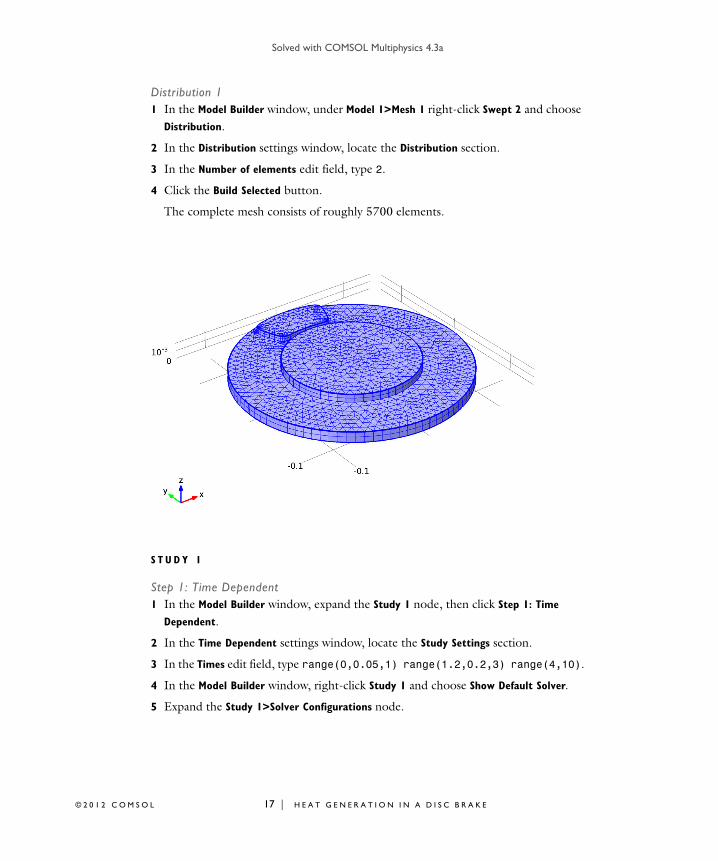
Distribution 11 Right-click Model 1>Mesh 1>Swept 1 and choose Distribution.

2 In the Distribution settings window, locate the Distribution section.

3 In the Number of elements edit field, type 2.


Swept 2In the Model Builder window, right-click Mesh 1 and choose Swept.

Wprod/diss t( ) Qprod/diss t'( ) t'd

0

t

=



© 2 0 1 2 C O

Distribution 11 In the Model Builder window, under Model 1>Mesh 1 right-click Swept 2 and choose

Distribution.

2 In the Distribution settings window, locate the Distribution section.

3 In the Number of elements edit field, type 2.


The complete mesh consists of roughly 5700 elements.

S T U D Y 1

Step 1: Time Dependent1 In the Model Builder window, expand the Study 1 node, then click Step 1: Time

Dependent.

2 In the Time Dependent settings window, locate the Study Settings section.

3 In the Times edit field, type range(0,0.05,1) range(1.2,0.2,3) range(4,10).

4 In the Model Builder window, right-click Study 1 and choose Show Default Solver.

5 Expand the Study 1>Solver Configurations node.



18 | H E

Solver 11 In the Model Builder window, expand the Study 1>Solver Configurations>Solver 1

node, then click Time-Dependent Solver 1.

2 In the Time-Dependent Solver settings window, click to expand the Absolute Tolerance section.

3 In the Tolerance edit field, type 1e-4.

4 Locate the Time Stepping section. From the Steps taken by solver list, choose Intermediate.

This setting forces the solver to take at least one step in each specified interval.

5 In the Model Builder window, right-click Study 1 and choose Compute.

R E S U L T S

The first of the two default plots displays the surface temperature of the brake disc and pad at the end of the simulation interval. Modify this plot to show the time just before releasing the brake.

Temperature1 In the Model Builder window, under Results click Temperature.

2 In the 3D Plot Group settings window, locate the Data section.

3 From the Time list, choose 1.8.


5 Click the Zoom Extents button on the Graphics toolbar.

Compare the result to the plot shown in Figure 2.

To compare the total heat produced and the heat dissipated, as done in Figure 5, follow the steps given below.

1D Plot Group 31 In the Model Builder window, right-click Results and choose 1D Plot Group.

2 In the 1D Plot Group settings window, click to expand the Title section.

3 From the Title type list, choose None.

4 Click to collapse the Title section. Locate the Plot Settings section. Select the x-axis label check box.

5 In the associated edit field, type Time (s).

6 Right-click Results>1D Plot Group 3 and choose Point Graph.

7 Select Point 1 only.



© 2 0 1 2 C O

8 In the Point Graph settings window, locate the y-Axis Data section.

9 In the Expression edit field, type log10(W_prod+1).

10 Click to expand the Coloring and Style section. Find the Line style subsection. From the Color list, choose Blue.

11 Click to expand the Legends section. Select the Show legends check box.

12 From the Legends list, choose Manual.


14 Right-click Results>1D Plot Group 3>Point Graph 1 and choose Duplicate.

15 In the Point Graph settings window, locate the y-Axis Data section.

16 In the Expression edit field, type log10(W_diss+1).

17 Locate the Coloring and Style section. Find the Line style subsection. From the Line list, choose Dashed.

18 Locate the Legends section. In the table, enter the following settings:


20 In the Model Builder window, right-click 1D Plot Group 3 and choose Rename.

21 Go to the Rename 1D Plot Group dialog box and type Dissipated and produced heat in the New name edit field.

22 Click OK.

Finally, follow the steps below to reproduce the plot in Figure 3.

Data Sets1 In the Model Builder window, under Results right-click Data Sets and choose Cut Line

3D.

2 In the Cut Line 3D settings window, locate the Line Data section.

3 In row Point 1, set z to 0.013.

4 In row Point 2, set x to -0.047.

5 In row Point 2, set y to 0.1316.

6 In row Point 2, set z to 0.013.

Legends

log10(W_prod+1), heat produced

Legends

log10(W_diss+1), heat dissipated



20 | H E


8 In the Model Builder window, right-click Data Sets and choose More Data

Sets>Parametric Extrusion 1D.

9 In the Parametric Extrusion 1D settings window, locate the Data section.

10 Click and Shift-click in the list to select all time steps from 0 through 3 s.

2D Plot Group 41 In the Model Builder window, right-click Results and choose 2D Plot Group.

2 Right-click 2D Plot Group 4 and choose Surface.

3 In the Surface settings window, locate the Coloring and Style section.

4 From the Color table list, choose ThermalLight.

5 Right-click Results>2D Plot Group 4>Surface 1 and choose Height Expression.

6 Right-click 2D Plot Group 4 and choose Rename.

7 Go to the Rename 2D Plot Group dialog box and type Temperature profile vs time in the New name edit field.

8 Click OK.


solved with comsol multiphysics 4.3a heat … with comsol multiphysics 4.3a ... heat transfer...

Documents