peak to average power ratio reduction schemes and ...sachin.c/me_report_final_draft.pdf · peak to...
TRANSCRIPT

Peak to Average Power Ratio Reduction Schemesand
Synchronization Algorithms for OFDM Based Systems
A Project ReportSubmitted in Partial Fulfillment of the� ��������� ����������������������
in � ������������! "�#�$�%�&�'�$(�by
SACHIN CHAUDHARI
Project Guide : Prof. K.V.S.HARI
Department of Electrical Communication EngineeringIndian Institute of Science
Bangalore-560012India
July 2004

Acknowledgments
I am greatly indebted to my guide Prof. K.V.S.Hari for his help and support throughout the course
of this project.
I would like to thank Joby, Bhavani, Vijay, Avinash, Deepak and Abhishek (SSP labmates) for
their help and discussions during the course of project. I would like to thank my friends Tanmay,
Ajay, Rupesh, Pankaj and Vibhor for giving me a great time at IISc.
I am thankful to my parents, my sister Shweta and my best friend Kiran for their love, and support.
i

Abstract
The relation of upper bound on Peak to Average Power Ratio (PAPR) with input constellation PAPR
is derived for general constellation and it is shown that upper bound on PAPR is greater for QAM as
compared to PSK of same order. A “pulse shaping scheme” is proposed for reduction of upper bound
on PAPR. An analytical expression for reduction in upper bound is obtained in terms of pulse shaping
weights and it is shown that more the variation in weights, more is the reduction.
Interleaved OFDM (IOFDM) was proposed to increase code rate without increasing PAPR. IOFDM
is studied from point of view of PAPR reduction while keeping code rate constant. Also IOFDMis shown to be superset of OFDM and Single Carrier Frequency Division Equalization (SC-FDE).
IOFDM can be used for trading with respect to number of subcarriers to get best of OFDM and SC-
FDE. IOFDM is shown to be better then most of the present scheme in terms of PAPR reduction,
complexity, and redundancy added. Block OFDM is proposed and compared with IOFDM to study
role of interleaving with regards to complexity.
A simple and efficient scheme “Tone based Integer Frequency Offset (IFO) Estimation“ is pro-
posed for IFO estimation. A modification is proposed which improves the performance in ISI case.
A detailed mathematical analysis is presented and the expression for Probability of error for most
general case is derived. Later it is compared with present algorithms in literature. It is also shown
how the proposed scheme is used in conjunction with Schmidl Cox Algorithm (SCA) for overall
synchronization and channel estimation in OFDM.
ii

List of Abbreviations
ACI Adjacent Carrier Interference
AWGN Additive White Gaussian Noise
BER Bit Error Rate
BOFDM Block Orthogonal Frequency Division Multiplexing
CFO Carrier Frequency Offset
CIR Channel Impulse Response
CP Cyclic Prefix
CCDF Complimentary Cumulative Distribution Function
DFT Discrete Fourier Transform
FFT Fast Fourier Transform
FIR Finite Impulse Response
HPA High Power Amplifier
IBI Inter Block Interference
ICI Inter Carrier Interference
IDFT Inverse Discrete Fourier Transform
IFFT Inverse Fast Fourier Transform
IFO Integer Frequency offset
IOFDM Interleaved Orthogonal Frequency Division Multiplexing
ISI Inter Symbol Interference
ML Maximum Likelihood
MZB Minn Zeng Bhargava (algorithm)
OFDM Orthogonal Frequency Division Multiplexing
PAPR Peak to Average Power Ratio
PN Pseudo NoisePSK Phase Shift Keying
PTS Partial Transmit Sequence
iii

iv
QAM Quadrature Amplitude Modulation
QPSK Quadrature Phase Shift Keying
SC-FDE Single Carrier Frequency Domain Equalization
SCA Schmidl Cox Algorithm
SLM Selected Mapping
SNR Signal to Noise Ratio

List of Symbols
capital with bold
face
Matrix
)+*-,�.Hermitian)+*-,0/Transpose)+*-,�1Conjugate)+*-,32&4Inverse5 6Estimate of
6a Vector
67 Linear convolution operation8�9 Input Constellation PAPR:Phase difference between two halves of first training symbol:�;Phase of <0=?> subcarrier@ Timing OffsetASize of correlating block in SCA (and its value is N/2)B3CED�FG9 Fractional frequency offset normalized to subcarrier spacingH )JI�KML&NO,Gaussian random variable with mean
Iand variance
LPNQ�R SUTVSzero matrixW R SUTVSidentity matrixXZY
Actual frequency offsetXZ[Frequency offset normalized to subcarrier spacingXZ[ ;Integer Frequency Offset\O]-^G_` a =?> rotation factor in PTS-OFDM
c pulse shaping vector in Proposed Pulse Shaping Scheme
d ]-b_ c =?> rotation vector in SLM-OFDM[Subcarrier index (Discrete Frequency Domain)[ ;Index of subcarrier on which data corresponding to IFO training
symbol is send
v

vi
[�d; Index of subcarrier on which data corresponding to IFO training
symbol is expected after occurrence of IFO at receivere Number of subcarriers on which data is send in IFO training sym-
bol of proposed scheme.f Corresponds to f =?> block
sSgTih
Input vector to IFFT at the transmitterjDiscrete time indexj 9 Continuous time indexk ) j , AWGN
xSgTih
Output vector of IFFT at transmitter
y i. In chapter 2,3,4, and 5, l Tihreceived vector at receiver.
ii. In chapter 6 and 7,SmTnh
vector input to FFT at receivero )qpr,Metric for IFO estimation in SCAs ) [ ,Metric for IFO estimation in proposed scheme (Tone based)t�u�v wyx T wyx
Precoding block diagonal matrix in IOFDM) S zwyx ,{
Diagonal matrix with (k,k) entry as channel transfer function for[ =?> subcarrier| R SgTVSpoint FFT matrix}P~��
Subcarrier spacing} D )J�&, CDF of random variable �� 2&� wyx T wyxPreprocessing Block diagonal matrix in IOFDM��� l T l channel convolution matrix� 4 l T l Inter block interference matrix� ) [ ,
Channel transfer function value at[ =?> subcarrier�� SgTVS
Circulant matrix with entry as � ) fV� [ ,�,xNumber of subcarrier in IOFDM�Upperbound on channel order� ; wyx T wyx
Interleaving matrix� u�v wyx T wyxPermutation matrixl Length of total OFDM symbol after CP additionl )���,
Timing metric for SCA at� =?> instantS
Number of Subcarriers in OFDMS pLength of Cyclic PrefixwInterleaving Factor in IOFDMw�;Instantaneous PAPR

vii
wP~Average power of OFDM symbol (excluding CP)wy�Probability of correct estimation of IFOw��Probability of error in estimation of IFOw�� ~�� w��
when data is sent on e subcarriers in proposed scheme for IFO
estimationw��Worst case PAPRw �����Worst case PAPR for given value of c in Pulse Shaping Scheme for
PAPR��� u SgT l Cyclic prefix removal matrix� e Case of Proposed scheme in which data has been sent on e sub-
carriers and zeroes on rest of the subcarriers�Time duration of OFDM symbol (without CP)� ~Time duration of one input symbol to IDFT� � u l TVS
Cyclic prefix addition matrix Number of distinct pseudo random, but fixed vector in SLM-
OFDM¡Number of pairwise disjoint blocks in PTS-OFDM¢ F Number of allowed phase angle in PTS-OFDM£ ) [ ,DFT of ¤ ) j , at receiver for chapter 6, and 7¢ ) [ ,DFT of k ) j , at receiver for chapter 6, and 7¢ 4 ) [ , Cyclically shifted
¢ ) [ ,

Contents
1 Introduction 11.1 OFDM . . . . . . . . . . . . . . . . . . . . . . . . . . . . . . . . . . . . . . . . . . 1
1.2 Motivation for Present Work . . . . . . . . . . . . . . . . . . . . . . . . . . . . . . 1
1.2.1 PAPR . . . . . . . . . . . . . . . . . . . . . . . . . . . . . . . . . . . . . . 1
1.2.2 Synchronization . . . . . . . . . . . . . . . . . . . . . . . . . . . . . . . . 21.3 Contribution of this project . . . . . . . . . . . . . . . . . . . . . . . . . . . . . . . 2
1.3.1 PAPR . . . . . . . . . . . . . . . . . . . . . . . . . . . . . . . . . . . . . . 2
1.3.2 Synchronization . . . . . . . . . . . . . . . . . . . . . . . . . . . . . . . . 2
1.4 Organization of Project Report . . . . . . . . . . . . . . . . . . . . . . . . . . . . . 3
2 OFDM 42.1 Generation of OFDM signal . . . . . . . . . . . . . . . . . . . . . . . . . . . . . . 4
2.2 OFDM system . . . . . . . . . . . . . . . . . . . . . . . . . . . . . . . . . . . . . . 5
2.3 Important Remarks . . . . . . . . . . . . . . . . . . . . . . . . . . . . . . . . . . . 8
3 PAPR 93.1 Introduction . . . . . . . . . . . . . . . . . . . . . . . . . . . . . . . . . . . . . . . 9
3.2 Distribution of PAPR . . . . . . . . . . . . . . . . . . . . . . . . . . . . . . . . . . 9
3.3 Factors Affecting PAPR . . . . . . . . . . . . . . . . . . . . . . . . . . . . . . . . . 11
3.4 PAPR Reduction Schemes . . . . . . . . . . . . . . . . . . . . . . . . . . . . . . . 13
3.4.1 Signal Distortion Techniques . . . . . . . . . . . . . . . . . . . . . . . . . 13
3.4.2 Selected Mapping . . . . . . . . . . . . . . . . . . . . . . . . . . . . . . . . 13
3.4.3 Partial Transmit Sequences . . . . . . . . . . . . . . . . . . . . . . . . . . . 15
3.4.4 Complementary Golay Sequences . . . . . . . . . . . . . . . . . . . . . . . 17
3.4.5 Proposed Scheme : Pulse Shaping for PAPR reduction . . . . . . . . . . . . 17
4 SC-FDE and IOFDM 214.1 SC-FDE . . . . . . . . . . . . . . . . . . . . . . . . . . . . . . . . . . . . . . . . . 21
4.1.1 Introduction . . . . . . . . . . . . . . . . . . . . . . . . . . . . . . . . . . . 21
4.1.2 Comparison between SC-FDE and OFDM . . . . . . . . . . . . . . . . . . . 22
viii

CONTENTS ix
4.1.3 SC-FDE Design-II . . . . . . . . . . . . . . . . . . . . . . . . . . . . . . . 234.2 IOFDM . . . . . . . . . . . . . . . . . . . . . . . . . . . . . . . . . . . . . . . . . 23
4.3 Generalized view of IOFDM . . . . . . . . . . . . . . . . . . . . . . . . . . . . . . 29
4.4 Block OFDM (BOFDM) . . . . . . . . . . . . . . . . . . . . . . . . . . . . . . . . 31
4.5 Importance of IOFDM . . . . . . . . . . . . . . . . . . . . . . . . . . . . . . . . . 31
5 Synchronization 345.1 Introduction . . . . . . . . . . . . . . . . . . . . . . . . . . . . . . . . . . . . . . . 34
5.1.1 Sensitivity to Carrier Frequency Offset (CFO) . . . . . . . . . . . . . . . . . 34
5.1.2 Sensitivity to Timing Errors . . . . . . . . . . . . . . . . . . . . . . . . . . 35
5.2 Synchronization Schemes for OFDM . . . . . . . . . . . . . . . . . . . . . . . . . . 36
5.2.1 Schmidl Cox Algorithm (SCA) . . . . . . . . . . . . . . . . . . . . . . . . 36
5.2.1.1 Symbol Synchronization . . . . . . . . . . . . . . . . . . . . . . 37
5.2.1.2 Carrier Frequency Offset (CFO) Estimation . . . . . . . . . . . . 40
5.2.2 Minn Zeng Bhargava (MZB) Algorithm . . . . . . . . . . . . . . . . . . . . 42
5.2.2.1 Sliding Window Method (Method A) . . . . . . . . . . . . . . . . 42
5.2.2.2 Training Symbol Method (Method B) . . . . . . . . . . . . . . . . 43
5.2.2.3 Simulations and Discussion . . . . . . . . . . . . . . . . . . . . . 44
6 Proposed Scheme : Tone based IFO estimation 476.1 Some Observations for Proposed Scheme . . . . . . . . . . . . . . . . . . . . . . . 48
6.2 Mathematical Analysis . . . . . . . . . . . . . . . . . . . . . . . . . . . . . . . . . 49
6.2.1 Data Model 1 : AWGN Channel . . . . . . . . . . . . . . . . . . . . . . . . 496.2.2 Data Model 2 : ISI Channel . . . . . . . . . . . . . . . . . . . . . . . . . . 52
6.3 Simulation Results and Observation . . . . . . . . . . . . . . . . . . . . . . . . . . 54
6.4 Modification to the Proposed Scheme for ISI case (Multitone) . . . . . . . . . . . . 55
6.4.1 Mathematical Analysis . . . . . . . . . . . . . . . . . . . . . . . . . . . . . 56
6.4.2 Simulation Results and Observation . . . . . . . . . . . . . . . . . . . . . . 58
6.5 Comparison between the proposed schemes and existing schemes . . . . . . . . . . 58
6.5.1 Performance . . . . . . . . . . . . . . . . . . . . . . . . . . . . . . . . . . 60
6.5.2 Computation Complexity . . . . . . . . . . . . . . . . . . . . . . . . . . . 61
6.5.3 Frequency Acquisition Range . . . . . . . . . . . . . . . . . . . . . . . . . 62
6.5.4 Number of Training symbol required . . . . . . . . . . . . . . . . . . . . . 62
6.6 Performance of Multitone scheme for timing synchronization and fractional frequency
offset . . . . . . . . . . . . . . . . . . . . . . . . . . . . . . . . . . . . . . . . . . 62
7 Conclusions 65

List of Figures
2.1 OFDM Transmitter . . . . . . . . . . . . . . . . . . . . . . . . . . . . . . . . . . . 5
2.2 OFDM Receiver . . . . . . . . . . . . . . . . . . . . . . . . . . . . . . . . . . . . 7
3.1 Plot of signal power of IFFT output for 16 channel OFDM signal, modulated with
same initial phase for all subchannels and average power=1 . . . . . . . . . . . . . . 10
3.2 CCDF forS
=16, 32, 64, 128 . . . . . . . . . . . . . . . . . . . . . . . . . . . . . 11
3.3 Block diagram for SLM-OFDM . . . . . . . . . . . . . . . . . . . . . . . . . . . . 14
3.4 CCDF curves (forS
=128) for
nos. of IDFT in SLM-OFDM and¡
nos. of IDFT
in PTS-OFDM with¢ F =4. . . . . . . . . . . . . . . . . . . . . . . . . . . . . . . . 15
3.5 Block diagram for PTS-OFDM . . . . . . . . . . . . . . . . . . . . . . . . . . . . . 16
3.6 Pulse shaping for PAPR reduction . . . . . . . . . . . . . . . . . . . . . . . . . . . 18
3.7 Plot ofw�;
for two ’c’ vectors (variation in�O¥
of fig.(a) is more as compared to fig.(b)) 19
4.1 Block Diagram for SC-FDE . . . . . . . . . . . . . . . . . . . . . . . . . . . . . . 22
4.2 Co-existence of SC-FDE and OFDM . . . . . . . . . . . . . . . . . . . . . . . . . . 23
4.3 SC-FDE Design-II . . . . . . . . . . . . . . . . . . . . . . . . . . . . . . . . . . . 23
4.4 PAPR for SC-FDE design-II . . . . . . . . . . . . . . . . . . . . . . . . . . . . . . 24
4.5 IOFDM transmitter . . . . . . . . . . . . . . . . . . . . . . . . . . . . . . . . . . . 25
4.6 IOFDM receiver . . . . . . . . . . . . . . . . . . . . . . . . . . . . . . . . . . . . . 25
4.7 Matrix model of IOFDM transmitter . . . . . . . . . . . . . . . . . . . . . . . . . . 26
4.8 Interleaving scheme for IOFDM . . . . . . . . . . . . . . . . . . . . . . . . . . . . 27
4.9 Matrix model for IOFDM receiver . . . . . . . . . . . . . . . . . . . . . . . . . . . 29
4.10 Simplified Block Diagrams of OFDM, SC-FDE, and IOFDM systems . . . . . . . . 30
4.11 Block OFDM . . . . . . . . . . . . . . . . . . . . . . . . . . . . . . . . . . . . . . 31
4.12 Comparison of complexity for IOFDM and BOFDM . . . . . . . . . . . . . . . . . 33
5.1 SNR degradation in dB Vs normalized frequency offset for (a) 64 QAM ( ¦ ~$§ S�¨ =19
dB) (b) 16 QAM ( ¦ ~G§ S©¨ =14.5 dB) (c) QPSK ( ¦ ~'§ S�¨ = 10.5 dB) . . . . . . . . . . . 35
5.2 Example of OFDM with 3 subcarriers showing the earliest and latest possible timing
instants that do not cause ISI or ICI. . . . . . . . . . . . . . . . . . . . . . . . . . . 36
5.3 Constellation Diagram with a timing error of� § h«ª
before and after phase correction 37
x

LIST OF FIGURES xi
5.4 Example of Timing Metric for AWGN channel (SNR=10 dB,S
=1024) . . . . . . . 385.5 Mean and variance at correct and incorrect timing instant for ISI channel . . . . . . . 40
5.6 Performance of frequency offset estimator (fractional + integer part) for an exponen-
tial Rayleigh channel with N=1024 . . . . . . . . . . . . . . . . . . . . . . . . . . . 42
5.7 Timing Metric of SCA and MZB under no noise and distortion condition . . . . . . . 44
5.8 mean and variance of SCA and MZB in AWGN . . . . . . . . . . . . . . . . . . . . 45
5.9 mean and variance of SCA and MZB in ISI . . . . . . . . . . . . . . . . . . . . . . 45
6.1w��
curves for Exponential Rayleigh (ISI) channel . . . . . . . . . . . . . . . . . . . 55
6.2w��
vs Timing Offset . . . . . . . . . . . . . . . . . . . . . . . . . . . . . . . . . . 56
6.3 Comparison of Multitone scheme for� h
,��¬
, and�®
. . . . . . . . . . . . . . . . . 59
6.4w��
Curves for Tone based scheme and SCA for different values of SNR andS
in
AWGN conditions . . . . . . . . . . . . . . . . . . . . . . . . . . . . . . . . . . . . 59
6.5w��
Curves for Multitone scheme and SCA for different values of SNR and N for
exponential decaying Rayleigh channel . . . . . . . . . . . . . . . . . . . . . . . . 60
6.6 Theoreticalw��
curves for SCA and Multitone scheme�P
. . . . . . . . . . . . . . 61
6.7 Mean and Variance at correct and incorrect timing instant forSmz¯hE° ¬±
and AWGN
case, e z . . . . . . . . . . . . . . . . . . . . . . . . . . . . . . . . . . . . . . . . 63
6.8 mean and variance at correct timing instant . . . . . . . . . . . . . . . . . . . . . . 64
6.9 Variance of Fractional FO error . . . . . . . . . . . . . . . . . . . . . . . . . . . . 64

List of Tables
4.2 Comparison of SLM, PTS, and IOFDM . . . . . . . . . . . . . . . . . . . . . . . . 32
6.1w��
for various values of SNR andS
in AWGN scenario (theoretical) . . . . . . . . 54
6.2w��
for various values of SNR andS
in AWGN scenario (simulation) . . . . . . . . 54
6.3 Relative Computation Complexity for SCA and Proposed Scheme . . . . . . . . . . 61
xii

Chapter 1
Introduction
1.1 OFDM
Orthogonal Frequency Division Multiplexing (OFDM) is a parallel data system. In OFDM [1],[2],
the wide band channel is divided into number of subchannels. These subchannels are permitted to
overlap in frequency domain with specific orthogonality constraints imposed to facilitate separation of
subchannels at the receiver. The serial data symbols are divided into parallel streams, then modulating
each parallel stream onto a separate subchannel. The symbol rate on each subchannel is lower than
overall symbol rate. Due to lower symbol rate on each subchannel, each subchannel looks like a flat
fading channel. OFDM has the advantage of spreading out the burst errors caused by additive burst
noise randomly so that the distortion of several adjacent symbols is avoided. OFDM has the additional
advantage of spreading out the symbol interval thereby reducing the ISI caused due to delay spread.
Therefore OFDM is an effective technique for combating multipath fading and for high data rate
transmission.
1.2 Motivation for Present Work
1.2.1 PAPR
Due to large number of subcarriers, the OFDM signal has large dynamic range with large Peak to
Average Power Ratio (PAPR). When considering a system with transmitting power amplifier, the non-
linear distortions and peak amplitude limiting introduced by the High Power Amplifier (HPA) will
produce intermodulation between the different carriers and introduce additional interference into the
system. This additional interference leads to an increase in Bit Error Rate (BER) of the system. One
way to avoid such non-linear distortions and keep a low BER is by forcing the amplifier to work in
its linear region. Unfortunately such solution is not power efficient and thus not suitable for wireless
communications.
Hence there is need for reducing PAPR of transmitted signal. Several techniques have appeared
1

CHAPTER 1. INTRODUCTION 2
in literature [11] to [21] and few are proposed.
1.2.2 Synchronization
Synchronization is an important step that must be performed at the receiver in OFDM systems, be-
fore an OFDM receiver starts demodulating subcarriers. Synchronization of an OFDM signal requires
finding the symbol timing and carrier frequency offset. Symbol timing for an OFDM is significantlydifferent than for a single carrier signal, since there is not an “eye opening” where a best sampling
time can be found. Rather there are hundreds of samples per OFDM symbol as number of samples
is directly proportional to number of subcarriers. There is some tolerance for symbol timing errors
when a cyclic prefix is used to extend the symbol. But synchronization of carrier frequency at the re-
ceiver must be done accurately, failing which, there will be loss of orthogonality between subcarriers
resulting in performance degradation.
Many papers on the subject of synchronization for OFDM have appeared in literature [22] to [27]
in recent years. A scheme has been proposed for integer frequency offset.
1.3 Contribution of this project
1.3.1 PAPR
1. The dependency of PAPR on input constellation (through 8(9 ) is shown and corresponding ex-
pression forw �
is obtained for general constellation.
2. A new scheme, called “Pulse Shaping Scheme”, is proposed for PAPR reduction. An analytical
expression for reduction in upperbound of PAPR is obtained in terms of pulse shaping weights.
3. IOFDM is reviewed from PAPR reduction point of view for constant code rate. Also it is
shown that IOFDM is superset of OFDM and Single Carrier Frequency Domain Equalization
(SC-FDE). IOFDM is compared with some of the schemes present in literature.
4. Block OFDM is proposed which has similar structure to that of IOFDM (but without interleav-
ing and minor differences). It is shown that BOFDM is also superset of OFDM and SC-FDE.Performance comparison of BOFDM and IOFDM is carried out.
1.3.2 Synchronization
1. A new scheme, called " Tone based Integer Frequency Offset estimation", is proposed for Inte-
ger Frequency Offset Estimation. Modification was suggested for the proposed scheme whichgreatly improves the performance of the proposed scheme. A detailed mathematical analysis
has been presented and Probability of error (w��
) expression for ISI and AWGN channel has
been derived. The proposed scheme is compared with other scheme in literature. Later it is
shown that the proposed scheme is used effectively with the existing algorithm called Schmidl

CHAPTER 1. INTRODUCTION 3
Cox Algorithm for overall synchronization i.e. timing, fractional frequency offset and integerfrequency offset.
1.4 Organization of Project Report
The project report is organized as follows. In chapter 2, conventional OFDM is described. In
chapter 3, PAPR is introduced and factors affecting PAPR are discussed in detail. Some PAPR re-
duction schemes are also discussed in the same chapter. In chapter 4, Interleaved OFDM and Single
Carrier Frequency Domain Equalization systems are discussed. In Chapter 5, issues regarding Syn-
chronization are discussed followed with the discussion on existing Synchronization Scheme. In
chapter 6, a scheme is proposed for Integer Frequency Offset (IFO) estimation and compared with
existing scheme. Chapter 7 concludes the current work.

Chapter 2
OFDM
2.1 Generation of OFDM signal
An OFDM signal consists of sum of subcarriers that are modulated by using phase shift keying
(PSK) or quadrature amplitude keying (QAM).S
number of such symbols are then fed to IDFT
through serial to parallel converter whereS
is number of subcarriers. If ² � K ² 4 KE³E³E³OK ² R 2&4 areS
complex QAM (or PSK) symbols, then output of the IDFT are
�P) j , z h´ SR 2&4µ¥'¶ � ² ¥·��¸+¹�º$»
�¼ j z½° K h KE³E³E³K S � h (2.1)
They are then converted to serial stream by parallel to serial (P/S) converter. The block ofS
output
symbols from parallel to serial converter make up one OFDM symbol. If� ~
is the time duration of
one input symbol to IDFT, then the total duration of a single OFDM symbol is� z½S � ~
.
Note that the sinusoids of the DFT (or IDFT) form an orthogonal basis set and a signal in vector
space of the DFT (or IDFT) can be represented as linear combination of the orthogonal sinusoids.
Thus the IDFT at the transmitter maps an input signal onto a set of orthogonal subcarriers. Similarly
the transform DFT is used at the receiver to reverse the mapping of IDFT and signal from the sub-
carriers are combined to form an estimate of the source signal from the transmitter. Since the basis
function of DFT are uncorrelated, the correlation performed in DFT for the given subcarrier only
sees energy for that corresponding subcarrier. The energy from other subcarrier does not contribute
because they are uncorrelated. This separation of signal energy is the reason that OFDM subcarriers
spectrum can overlap without causing interference.
In practice OFDM systems are implemented using a combination of Fast Fourier Transform (FFT)
and Inverse Fast Fourier Transform (IFFT) that are mathematically equivalent versions of the DFT
and IDFT, but are computationally more efficient. Complexity of DFT isS N
whereas that of FFT isR NP¾J¿ p S .
4

CHAPTER 2. OFDM 5
x(n) u(n)
N 1N 1
s(n)
M 1
F P/SS/P THN cp u(n)s(n)
Figure 2.1: OFDM Transmitter
2.2 OFDM system
Figure 2.1 shows a discrete time baseband model of an OFDM transmitter. At the transmitter the
bit stream is mapped onto a complex symbol ² ) f , using any modulation scheme. The symbol stream
is then blocked into a parallel block stream s) f , , each block comprising
Ssymbols so that we have
s) f , zÁÀ ² ) f S ,GK ² ) f SÃÂÄh ,GKE³E³E³O³E³E³«K ² ) f SÁÂ!S � h ,0Å / . Here f denote the block index. The block
stream s) f , is then precoded using
SÆTySpoint IFFT matrix
| .R to yield so called time domain block
vector x) f , . Then redundancy of length
SÈÇis added to each block using cyclic prefix (
SÉÇis length
of Cyclic prefix andS ÇÉÊ �
, where�
is upperbound on channel order). The entries of the resulting
block are u) f , zËÀ c ) f l ,GK c ) f l ÂÌh ,GKE³E³E³K c ) f l  l � h ,0Å?/ , where l z½S¯ÂnS p
. This block is
then transformed to serial stream c ) f , , upconverted to RF and is transmitted through antenna.The following equations represent the precoding and cyclic prefix (CP) insertion operation :
x) f , z | .R s
) f , (2.2)
u) f , z � � u
x) f , (2.3)
where� � u
is l TÍSmatrix given by
� � u zÉÀ | � u K | Åq.,| � u
isSÎTÏS Ç
matrix formed by the lastS�Çrows of
| R. The frequency selective propagation can modeled as an FIR filter with the channel
impulse response (CIR) column vector hzÐÀ � � K � 4 KE³E³E³«K ��Ñ Å / and additive white gaussian noise w
) f ,of variance
LÒN. We assume that we have perfect knowledge of CIR at the receiver and no CIR is
available at the transmitter.
Letting y) f , be the f =?> received block, with y
) f , being the signal at the receiver front end after
downconversion from RF and blocking from serial to parallel, we can represent the transmit receiveequations as
y) f , z �ÔÓ
u) f , Â � � u
) fV� h , Â w) f , (2.4)

CHAPTER 2. OFDM 6
where��Ó
is l T l lower triangular Toeplitz filtering matrix given as
�ÔÓ zÕÖÖÖÖÖÖÖÖ×
� ) ° , ° ° ³E³E³ °... � ) ° , ° ³E³E³ °
� ) � , ³E³E³ . . .³E³E³ ...
.... . .
³E³E³ . . . °° ³E³E³ � ) � ,سE³E³ � ) ° ,
ÙEÚÚÚÚÚÚÚÚÛ
and� � represent Inter-Block Interference (IBI) l T l upper triangular Toeplitz filtering matrix
given by
� � zÕÖÖÖÖÖÖÖÖ×
° ³E³E³ � ) � , ³E³E³ � ) h ,...
. . . ° . . . °° ³E³E³ . . .³E³E³ � ) � ,
......
.... . .
...° ³E³E³ ° ³E³E³ ° °
ÙEÚÚÚÚÚÚÚÚÛ
and w) f , =
À k ) f l ,GKE³E³E³K k ) f l  l � h ,0Å?/ denotes AWGN vector. At the receiver, cyclic prefix is
removed by using receive matrix�Z� u zÐÀÜQ�RÞÝrR ß W R Å
to give IBI free block given by
àx) f , z ��� u
y) f , (2.5)z �á� u ��Ó � � u
x) f ,  �á� u w
) f , (2.6)
Note that IBI inducing matrix has been eliminated by�Ô� u
( from equations 2.4,2.6, and�Z� u � � zQ�RÞÝrâ
). Thus redundancy is used to mitigate multipath effectively. Now ã� z ��� u �ÔÓ � � uisSÃTÉS
circulant matrix with its (n,k) entry as � )�) fÏ� [ , e ¿ � S , . This shows that by inserting CP (through� � umatrix ) and removing it at the receiver (using
�Ô� u), the linear convolution channel with IBI is
converted to circular one without IBI. Therefore equation 2.6 becomes
àx) f , z ã� x
) f ,  ��� u w) f , (2.7)
Equalization of OFDM with CP transmission relies on following important property of circulant ma-
trix
Diagonalization of circulant matrices : AnSäTÏS
circulant matrix ã� can be diagonalized by
pre and post multiplication with FFT and IFFT matrices of sizeS
i.e.

CHAPTER 2. OFDM 7
y(n)
N 1 N 1
P/S
N 1
N 1
M 1
s(n)
q(n)x(n) y(n)F
DET
D−1
NS/P
y(n)R
cp
s(n)
z(n)
DET=detector
Figure 2.2: OFDM Receiver
|åR ã� | .R z {(2.8)
where{ z � < 6�p À �æ� K � 4 KE³E³E³«³E³E³OK � R 2&4 Å with
� ¥ z � ) [ , zèç Ñé ¶ � � é � 2�N�ê ¥ éìë R denoting the channel
transfer function for the[ =?> subcarrier. Note
{isSmTVS
matrix. íNow equation 2.7 can be written asà
x) f , z | .R { |åR x
) f , Â � � u w) f , (2.9)
Taking FFT of both sides and noting that xz | .R s
) f , gives
q) f , z {
s) f , Â |�R � � u w
) f , (2.10)
Taking{ 2&4
(assuming{
is invertible which is possible if and only if the channel transfer function
does not have zero on FFT grid i.e.� ¥�îz½° ï [ñð À ° K S � h Å ), we get
z) f , z
s) f , Â { 2&4 | R � 9 � w ) f , (2.11)
Finally passing z) f , through the detector we get
às) f , , approximation to s
) f , . Receiver diagram is
shown in figure 2.2.

CHAPTER 2. OFDM 8
2.3 Important Remarks
1. We can use Zero Padding [1],[9],[10] instead of cyclic prefix at the transmitter, and do overlap
add operation at the receiver, the same transformation of the channel convolution matrix froma toeplitz to circulant is obtained. One difference between cyclic prefix and the zero pad is that
the redundancy in case of cyclic prefix is data dependent, while in case of zero padding it is data
independent and hence can be used for channel estimation. Moreover if one does not discard
the zero pad at the receiver, the equivalent channel convolution matrix is tall Toeplitz which is
guaranteed to be full rank as long as all of the channel taps are not zero. This system is resistant
to channel nulls.
2. The role of IFFT at the transmitter can also be interpreted thus : The modulated individual
OFDM subcarriers can be viewed as the spectrum of the signal to be transmitted and hence one
needs an IFFT to transform the ’spectrum’ to time domain to transmit it through channel.
3. The equalized signal/decision vector is given by equation 2.11. It can be seen that the noise
vector is multiplied by the inverse of the diagonal matrix{
, comprising the eigenvalues of theequivalent channel convolution matrix ã� . If one or more eigenvalues are close to zero, then
the noise will be amplified. In other words, the channel must not have zeros on any of the
subcarriers.
4. The code rate of the OFDM system is the ratio between the number of useful symbols to the
total number of symbols transmitted. Hence the code rate is given byRR#ò&R ß . The number of
redundant symbol is greater than equal to upperbound on the length of CIR.
5. OFDM works with the assumption that the CIR does not change in the time required to transmitSÃÂ!S Çsymbols. If the CIR changes within this time, then the equalization will not work at
the receiver and the block ofSóÂôSõÇ
symbols will be lost.

Chapter 3
PAPR
3.1 Introduction
An OFDM signal consists of number of independently modulated subcarriers, which can give large
peak to average power ratio (PAPR) when added up coherently. WhenS
signals are added with the
same phase they produce a peak power that isS
times their average power. This effect is illustrated
in figure 3.1 forS zöh«ª
case, for which the peak power is 16 times the average value. A large
PAPR brings disadvantage like an increased complexity of the analog to digital and digital to analog
converters and reduced efficiency of the RF power amplifier.
From equation 2.1 we know that OFDM signal (block ofS
symbols) is generated using input
symbols ² ) [ ,GK [ z½° K h KE³E³E³±K S � h as
�P) j , z h´ SR 2&4µ¥E¶ � ² ) [ , �3÷ N�ê ¥ = ë R j z½° K h KE³E³E³±K S � h (3.1)
Note that this definition of IFFT does not scale the input power i.e total input and output power of IFFT
are same. Same is the case with average input power and average output power of IFFT. Throughout
the report this normalized definitions are used for IFFT and FFT. Now instantaneous PAPR for above
case can be given by
w�; z øÉù±ú =�û �®) j , û N¦ À û �®) j , û N Å (3.2)
3.2 Distribution of PAPR
Assume that ² ) [ , are from QPSK, i.e. ² ) [ , ðýü � h K h K0þ�K � þ�ÿ . From the central limit theorem itfollows that for large values of
S, the real and imaginary values of
�P) j ,becomes Gaussian distributed,
9

CHAPTER 3. PAPR 10
0 2 4 6 8 10 12 14 160
2
4
6
8
10
12
14
16
t
|x(t)
|2
Figure 3.1: Plot of signal power of IFFT output for 16 channel OFDM signal, modulated with sameinitial phase for all subchannels and average power=1
each with variance 0.5. The amplitude of the OFDM signal therefore has a Rayleigh distribution while
the power distribution becomes Central chi-square distribution with two degrees of freedom and zero
mean with cumulative distribution given by
} )��%, z h � � 2�� (3.3)
We want complementary cumulative distribution (CCDF) function for the peak power per OFDM
symbol. Assuming the samples are mutually uncorrelated, the probability that PAPRw ;
is above
some threshold level can be written as
w ) w ;�� �%, z h � } )���, Rz h � ) h � � 2�� , R (3.4)
The CCDF forS
=16, 32, 64, 128 is plotted in figure 3.2.
The distribution of PAPR illustrates that symbols with high PAPR occurs less frequently. So it is
possible to deduce coding techniques to reduce PAPR by transmitting symbols with low PAPR only.
A different way to solve the PAPR problem is to remove the peaks at the cost of slight interference
that can be made as small as possible. Many schemes are based on bending the CCDF curves toward
left, and thus further reduce the probability of occurring of symbols with high PAPR. Some of them

CHAPTER 3. PAPR 11
6 7 8 9 10 11 12 13 14 15
10−10
10−8
10−6
10−4
10−2
Pr(
Xu>
Xo)
10 log10 Xo [dB]
CCDF plot of papr for OFDM for different N
N=16N=32N=64N=128
Figure 3.2: CCDF forS
=16, 32, 64, 128
are discussed later in this chapter (for example, Selected Mapping, Partial Transmit Sequences).
3.3 Factors Affecting PAPR
Before discussing the factors affecting PAPR, we will derive upperbound onw#;
. We call it worst
case PAPR and denote it byw �
. From equation 3.2
w ; z e 6%� = û �®) j , û N¦ À û �P) j , û N Å z e 6%� = 4R û ç R 2&4¥E¶ � ² ) [ , � ÷ N�ê ¥ = ë R û N¦ À û ² ) [ , û N Å� øÉù±ú=ç R 2&4¥E¶ � û ² ) [ , � ÷ N�ê ¥ = ë R û N¦ À û ² ) [ , û N Å � û R 2&4µ¥E¶ � 6 ` û N � S R 2&4µ¥E¶ � û 6 ` û N
z ç R 2&4¥E¶ � û ² ) [ , û N¦ À û ² ) [ , û N Å� øÉù±ú¥ S û ² ) [ , û N¦ À û ² ) [ , û N Å (3.5)
Thereforew �
is given by
w � z øÉù±ú¥ S û ² ) [ , û N¦ À û ² ) [ , û N Å (3.6)

CHAPTER 3. PAPR 12
Let us define 8r9 as
8 9 z øÉù±ú¥ û ² ) [ , û N¦ À û ² ) [ , û N Å (3.7)
It can be seen from the above equation that 8 9 is nothing but PAPR of the input constellation, so that
equation 3.6 can be written as
w � z S 8�9 (3.8)
Important factors on which PAPR depends are
1. � , number of subcarriers in OFDM system :PAPR depends linearly on
S(from equation 3.8). If we reduce
Sthen PAPR reduces, but code
rate also decreases (assuming channel order remains constant).
2. 8 � , Input constellation PAPR :PAPR is directly proportional to 8 9 (from equation 3.8). It is straight forward that 8 9 is more for
QAM as compared to PSK. In fact for any order PSK 8�9 zÁh. In case of QAM, 8�9 increases with
increasing order. So that we can write
w F � z 8 F � w �O~ ¥ (3.9)
wherew� F � is
w �for QAM,
w �O~ ¥isw �
for PSK, and 8 F � is 8r9 for QAM. In fact, the above equation
is true for arbitrary constellation given that they are fed the same sequences. Henceforth we will use
only PSK for discussion on PAPR.
3. Autocorrelation of data sequences :To see dependence of PAPR on out of phase aperiodic autocorrelation values on data sequences,
we state a theorem [11].
Theorem : Let the aperiodic autocorrelation coefficient be
� ) ¾ , z R 2 ¥µ¥E¶ 4 ² ) [ Â ¾ , ² 1 ) [ , Y ¿ � [ z½° K h KE³E³E³K S � hwith û ² ) [ , û N z h ï [ , then the peak factor is upper bounded by
w�; � h� ¬SR 2&4µ é ¶ 4 û � ) ¾ , û í (3.10)

CHAPTER 3. PAPR 13
From this equation 3.10,w �
for a allowed set of input sequences is given by
w � z øÉù±ú s) h#Â ¬S
R 2&4µ é ¶ 4 û � ) ¾ , û , (3.11)
This dependence of PAPR on autocorrelation of data sequence is exploited to reduce the PAPR by
using the sequences that have low autocorrelation coefficient for[ îz½°
. For example, Golay sequences
have been extensively used for reduction of PAPR and are discussed in next chapter. In fact equation
3.8 is special case of equation 3.10 with � ) ¾ , zËh ï [ z½° K h KE³E³E³±K S � h .3.4 PAPR Reduction Schemes
Several techniques [11]-[21] have been proposed for reducing PAPR. Some of them are discussed
in this chapter. The important factors while looking at different schemes are complexity, redundancy,
and reduction in PAPR.
3.4.1 Signal Distortion Techniques
This technique reduce the peak amplitude simply by nonlinearly distorting the OFDM signal at or
around the peaks. Examples of distortion techniques are clipping, peak windowing and peak cancel-
lation. The disadvantage is that by distorting the OFDM signal amplitude, a kind of self interference
is introduced, that degrades bit error rate (BER). Second disadvantage is that the nonlinear distortion
increases the level of out of band radiation. Details can be found in [2]. Their mention here is for
sake of completeness. Our main focus of the section will be on techniques that avoid or reduce the
occurrence of symbols with high PAPR. It is rightly said “ Prevention is Better than Cure”.
3.4.2 Selected Mapping
In a more general approach [14],[15], it is assumed that
statistically independent alternative
transmit sequences x]ìb_` represent the same information ( f denotes f =?> block). Then the one with
lowest PAPR (denoted as ` ) is selected for transmission. The probability that ` exceeds threshold
PAPR ( ¨ ) is approximately
w � ü ` � ¨ ÿ z ) h � ) h � � 2���� , R ,�� (3.12)
Because of the selected assignment of binary data to transmit signal, this principle is called selected
mapping.The block diagram of SLM-OFDM (Selected Mapping OFDM) is shown in figure 3.3.

CHAPTER 3. PAPR 14
d (U)
s (2)n
s (1) n
d (2)
d (1)
Selection
of
Desirable
Symbol
x (U)n
x (2)n
x (1) n
xns
n
sn
S/P Conversion
IDFT
IDFT
Coding
Interleaving
Mapping
SideInformation
IDFT
(U)
Figure 3.3: Block diagram for SLM-OFDM
A set of
markedly different distinct pseudo-random but fixed vectors d ]ìb_ z À � ]ìb_� K � ]-b_4 ,³E³E³
,� ]ìb_R 2&4 Å with� ]-b±_^ z � ÷��������� where
: ]ìb_^ ð À ° K ¬�� ,GK ° � a � S K h � c � must be defined. The
subcarriers vector s ` is multiplied subcarrier wise with each of the
vectors d ]ìb_ resulting in a set of different subcarrier vectors s
]-b_` with components
² ]ìb_`"! ^ z ² `#! ^ � ]-b_^ ° � a$� S K ° � c � (3.13)
Then all
alternative subcarrier vectors are transformed into time domain to get x]-b_` z&%"' } � ü
s]-b±_` ÿ
and finally the sequence�x ` with lowest PAPR ` is transmitted. Note that one of the alternative
subcarrier vectors can be unchanged original one.
The following comments are in order :
á Redundancy is introduced to inform the receiver which vector d was used for the generation of
transmitted OFDM signal in f =?> block. It is given by ( ~ é � z ¾�¿ p N bits per OFDM symbol.
á Complexity of this scheme is
– Transmitter : R N ¾�¿ p N Só ) � h , S
– Receiver :S  R N ¾�¿ p N S
– Total complexity :) Âýh , R N ¾�¿ p N Só S
á The value ofw �
has not reduced but its probability has gone down as CCDF curves have shifted
left side as shown in figure 3.4.

CHAPTER 3. PAPR 15
Figure 3.4: CCDF curves (forS
=128) for
nos. of IDFT in SLM-OFDM and¡
nos. of IDFT inPTS-OFDM with
¢ F =4.
3.4.3 Partial Transmit Sequences
In this scheme [13], [15], the subcarrier vectors s ` is partitioned into¡
pairwise disjoint subblocks
s]-^G_` K h � a � ¡ . All subcarrier positions in s
]-^G_` which are already represented in another subblock
are set to zero, so that s ` z ç*)^ ¶ 4 s]-^$_` . We introduce complex valued rotation factors
\�]ì^G_` z � ÷���� � �+where
: ]-^G_` ð À ° K ¬�� ,GK h � a � ¡ enabling a modified subcarrier vector
�s ` z )µ^ ¶ 4 \ ]ì^G_` s ]ì^G_` (3.14)
which represents the same information as s ` , if the setü \]-^$_` K h � a � ¡ ÿ
(as side information
is known for each f ). Clearly a joint rotation of all subcarriers in a subblock by the same angle:Ò]-^G_` z 6 � p() \O]-^G_` , is performed. To calculate x ` z,%#' } � ü s ]-^G_` ÿ, the linearity of IDFT is exploited
yielding
x ` z )µ^ ¶ 4 \ ]-^G_` %#' } � ü s ]ì^G_` ÿ z )µ^ ¶ 4 \ ]-^G_` x ]ì^G_` (3.15)
where the V set partial transmit sequences x]-^G_` z&%#' } � ü
s]-^G_` ÿ
have been introduced. Based on them
a peak value optimization is performed by suitably choosing the free parameters\ ]-^G_` . The
\ ]ì^G_` may be
chosen with continuous valued phase angles, but more appropriate in practical systems is a restriction

CHAPTER 3. PAPR 16
OptimizationPeak Value
IDFT
IDFT
IDFT
s
s
s x
x
x
xn
S/P Conversion
Coding
Mapping
Interleaving
(1)
(2)
(V)
SideInformation
(V)
(2)
(1)
n
n
n(1) n
(2)n
(V)n
b
b
b
n
n
n
Figure 3.5: Block diagram for PTS-OFDM
on finite set of¢ F allowed phase angles. The optimum transmit sequence is then transmitted which
is given by
�x ` z )µ^ ¶ 4 �\ ]ì^G_` �
x ` (3.16)
The PTS-OFDM (Partial Transmit Sequence OFDM) is shown in figure 3.5. Until now, pseudo-
random subblock partitioning has found to be best choice for PAPR reduction [13].
Similar to SLM scheme, in this case alsow �
(worst case PAPR) is not reduced but its probability
does reduce as shown from figure 3.4. Note that PTS can be interpreted as a structurally modified
special case of SLM if¢ ) 2&4F z
and d ]-b_ are chosen in accordance with the partitioning and all
the allowed rotation angle combinationsü \·]ì^G_` ÿ
. In PTS the choice\±]-^G_` ðÍü.- h K - þrÿ
(¢ F z ) is very
interesting for an efficient implementation, as actually no multiplication must be performed, when
rotating and combining the PTSs x]-^$_` to get the peak optimized transmit sequence
�x ` .
The following comments are in order
á Redundancy of ( � = ~ z ) ¡ � h , ¾�¿ p N ¢ F bits per OFDM symbol is needed.
á Complexity :
– Transmitter :¡ R NP¾�¿ p N S  ¡ S
– Receiver :R NP¾�¿ p N SóÂôS
– Total Complexity :) ¡ ½h ,') R NP¾J¿ p N Só S ,

CHAPTER 3. PAPR 17
á The value ofw �
has not reduced but its probability has gone down as CCDF curves have shiftedleft side as shown in figure 3.4.
3.4.4 Complementary Golay Sequences
Only few data sequences produce signals with high PAPR. With golay codes, we can generate
sequences that once modulated with, have PAPR limited to 3dB [2], [21].
A sequence x of lengthS
is said to be complementary to another sequence y if the following
conditions on the sum of autocorrelation function holds
R 2&4µ¥E¶ � )J� ¥ � ¥ ò ; Â ¤ ¥ ¤ ¥ ò ; , z ¬ S < zý° (3.17)z ° < îz½° (3.18)
There are very interesting relationships between Complementary Golay sequences and Reed Muller
code [21], using which, it is easy to design a block algorithm for coding input sequences into Comple-
mentary Golay Sequences. These sequences give PAPR of 3dB along with error correction capabilities
of Reed Muller codes. Code rate decreases exponentially asS
increases. The minimum distance be-
tween two different complementary codes of lengthS
isS § ¬
symbols, so it is possible to correctR / � h symbol errors orR N � h erasures. The Complementary Golay sequences are valid only for
phase modulations (PSK) and are not valid for QAM.
Complexity increases exponential withS
[2]. For OFDM systems with large number of subcar-
riers it may not be feasible to generate sufficient number of complementary codes with a length equal
to number of channels. To avoid this problem the total number of subchannels can be split into groups
of channels at the cost of reduced error correction capability, but this reduces PAPR and increases
coderate.
3.4.5 Proposed Scheme : Pulse Shaping for PAPR reduction
It has been seen in earlier section of this chapter, thatw �
is caused by the symbol with highest
power, when it occurs on all subcarriers in phase. One way to reduce the PAPR is to scale the inputs
that modulate the subcarriers differently.
With reference to figure 3.6, consider that all subcarriers are fed symbols) \ 4 K \ N ³E³E³ \ R , from
the same M-PSK constellation. Without loss of generality assume û \±¥ û zØh ï [¯ð À h K S Å. Here� 4 K � N KE³E³E³OK � R Ê ° are real pulse shaping coefficients (or weights). So we have
w ; z øÉù±ú= û � =Mû N¦ À û � = û N Å (3.19)

CHAPTER 3. PAPR 18
Ns
b 2
b 1
b N
2s
1s
c 1
cN
Nx
2x
1x
c 2
IFFT
Figure 3.6: Pulse shaping for PAPR reduction
where� = z 40 R ç R¥E¶ 4 ² ¥±� ÷ N�ê ¥ = ë R . Note that
� = 1 �P) j , and ² ¥ 1 ² ) [ , .¦ À û � =Mû N Å z ¦ À û ² ¥ û N Å2 û � 4 \ 4 û N Â ³E³E³ Â û � R \ R û NSz � N 4 Â ³E³E³ Â � N RS¦ À û � =Mû N Å z hS
Rµ¥'¶ 4 � N¥ (3.20)
Now, øæù±ú = û � = û N is caused when all the input symbols are in phase i.e.
\ 4 z \ N z ³E³E³ z \ R z \(3.21)
Therefore, we have
øÉù±ú= û � =Gû N z øÉù±ú=hS 33333 Rµ¥E¶ 4 ² ¥� ÷ N�ê ¥ = ë R 33333 N
z øÉù±ú=hS 33333 \ Rµ¥E¶ 4 �'¥±�G÷ N�ê ¥ = ë R 33333 N
z hS 33333 Rµ¥E¶ 4 �'¥ 33333 N (3.22)

CHAPTER 3. PAPR 19
0 1000 2000 3000 4000 5000 6000 7000 8000 9000 100000
10
20
30
40
50
60
70
no of realization
PA
PR
PAPRiPw
ckPAPRw
0 10 20 30 40 50 60 700
0.1
0.2
0.3
0.4
0.5
0.6
0.7
0.8
0.9
1
c(k)
or c
k
k
(a)
0 1000 2000 3000 4000 5000 6000 7000 8000 9000 100000
10
20
30
40
50
60
70
no of realization
PA
PR
PAPRiPw
ckPAPRw
0 10 20 30 40 50 60 700
0.2
0.4
0.6
0.8
1
1.2
c(k)
or c
k
k
(b)
Figure 3.7: Plot ofwP;
for two ’c’ vectors (variation in�O¥
of fig.(a) is more as compared to fig.(b))
Then upperbound onwP;
for given value of�E¥
’s (i.e c), (denoted asw k 9 ¥ ) can be written using equa-
tions 3.19, 3.20, 3.22, and 3.21 as
w k 9 ¥ z û ç �'¥ û N333 ç R¥E¶ 4 � N¥ 333 � S (3.23)
Equality holds only if� 4 z � N z ³E³E³ z � R .
w ; � w k 9 ¥ � w �(3.24)
So it can be seen from above equation that for a given c,w k 9 ¥ serves as new upper bound on
w ;that
is less than equal tow �
. Thus the upper bound on PAPR is reduced by a factor 4 z R65 ¼�87:9 9 ¹�] 5 ¼�87:9 9 � _ ¹ .Note that even if subcarriers are modulated by symbols from different constellations having dif-

CHAPTER 3. PAPR 20
ferent average power, it can be considered to be some constant times one common average powerw F ^ Ç and that constant can be absorbed in�O¥
. (Similar kind of results have been seen in [17] derived
in slightly different way, but we have derived it independently). The optimal power (or bit) loading
(water pouring), and channel equalization at the transmitter [1] can be used when CIR is available
at the transmitter and it can be seen when these schemes will have unequal��¥
’s, these schemes re-
duce PAPR. Reduction in PAPR depends on variation in coefficients�·¥
’s. More the variation, more
is the reduction in PAPR as can be seen from figure 3.7. If we are doing channel equalization at the
transmitter this will correspond to variation in channel frequency response.
The following comments are in order
á Code rate remains unchanged (i.e. same as OFDM without pulse shaping) if we use predeter-
mined c. Otherwise redundancy depends on variation in c (how fast c is changed w.r.t time and
how it is conveyed to receiver etc). In case of optimal power (or bit) loading and channel equal-
ization at transmitter,�«¥
’s are dependent on channel. Since channel is known at both receiver
and transmitter for this case, redundancy added will be zero.
á Complexity of the scheme is given as follows
– Transmitter :R N®¾�¿ p N S ÂôS
– Receiver :R NP¾�¿ p N SóÂôS
– Total Complexity :S ¾J¿ p N S Â ¬ S
á Upper bound on PAPR is reduced by the factor 4 .

Chapter 4
SC-FDE and IOFDM
4.1 SC-FDE
4.1.1 Introduction
A single carrier frequency domain equalization (SC-FDE) [18],[19] is a different system itself with
similar performance to OFDM, but has low PAPR and hence is discussed here.
An SC-FDE system transmits a single carrier modulated with QAM (or PSK) at high symbol
rate. Frequency domain linear equalization in an single carrier system is simply the frequency domain
analog of what is done in conventional time domain equalizer. For channels with severe delay spread,
FDE is computationally simpler than the corresponding time domain equalization for the same reason
OFDM is simpler, because equalization is performed on a block of data at a time and operation on this
block involve an efficient FFT operation and a simple channel inversion operation. When combined
with FFT processing and the use of a cyclic prefix, SC-FDE has same performance and low complexity
as OFDM system.
The SC-FDE system is shown in figure 4.1. Serial to parallel (S/P), parallel to serial (P/S) blocks,
RF sections are omitted for convenience.
Noting the similarity between block diagrams for OFDM system and that for SC-FDE, the analysis
for OFDM and SC-FDE are quite similar. Hence, we can directly write
z) f , z | .R { 2&4 | R � 9 ���ÔÓ � � u s
) f , Â | .R { 2&4 | R � 9 � w ) f , (4.1)
Noting that� 9 � � Ó � � u z | .R { |�R , we have
z) f , z
s) f , Â | .R { 2&4 |�R � 9 � w ) f , (4.2)
21

CHAPTER 4. SC-FDE AND IOFDM 22
N
HFF
cpR
z(n)
s(n)
s(n)
1N
1N
HM 1
FN
1NM 1
w(n)
D −1Tcp
Detector
Figure 4.1: Block Diagram for SC-FDE
4.1.2 Comparison between SC-FDE and OFDM
Advantages of SC-FDE as compared to OFDM are [18][19] :
1. Reduced PAPR as no IFFT at the transmitter. Now PAPR is in fact 8 9 . This allows the use of
less costly power amplifier.
2. Coding while desirable, is not necessary for combating frequency selectivity unlike non-adaptive
OFDM.
3. Frequency offset problem is not severe due to absence of multiple carriers.
4. Resistant to narrowband interference.
5. Transmitter complexity is reduced.
Disadvantages of SC-FDE as compared to OFDM [18][19] :
1. Receiver complexity has increased.
2. Optimal bit loading (Water Pouring) cannot be used.
3. Time domain impulsive noise causes error.
There may actually be an advantage in operating a dual mode system, wherein the base station uses
an OFDM transmitter and SC-FDE receiver and the subscriber modem uses an SC-FDE transmitter
and OFDM receiver as shown in figure 4.2. This arrangement of OFDM in downlink and SC-FDE inuplink has two potential advantages :
1. Concentrating most of the signal processing complexity at the hub or the base station. The hub
has two IFFT’s and one FFT while the subscriber has only one FFT.
2. The subscriber transmitter is SC-FDE and thus inherently more efficient in terms of power con-
sumption due to reduced power backoff requirements of the SC-FDE mode. This may reduce
the cost of a subscriber power amplifier.

CHAPTER 4. SC-FDE AND IOFDM 23
IFFTInvert Channel
Invert Channel
HUB END SUBSCRIBER END
IFFT FFTChannel
Channel CPFFT
CP
Det
Det
Downlink OFDM Transmitterat Hub
Uplink SC receiver at Hub
Downlink OFDM Receiver at subscriber
Uplink SC transmitter at subsciber
Figure 4.2: Co-existence of SC-FDE and OFDM
w(n)
HM 1
cpRz(n)s(n)
1NDetector
s(n)
1NF
N N
HFFD −11N
M 1
Tcp
Figure 4.3: SC-FDE Design-II
4.1.3 SC-FDE Design-II
For SC-FDE, design-II as shown in figure 4.3 is proposed here, in which FFT, Equalizer, and IFFT
can be shifted to transmitter. Motivation for design II is that if we use the transmitter of original
SC-FDE and receiver of design-II at subscriber end and corresponding receiver and transmitter at hub
end, then complexity of subscriber will reduce significantly. But the disadvantage of design-II is that
PAPR increases considerably and is almost similar to that of OFDM. The simulation results for PAPR
of the SC-FDE design-II are shown in figure 4.4.
4.2 IOFDM
In case of OFDM if the channel is constant for a time longer than what it takes to transmit one block
ofS Â�S�Ç
symbols, then one is sending more redundant symbols than required i.e. the code rate is

CHAPTER 4. SC-FDE AND IOFDM 24
0 20 40 60 80 100 120 140 160 180 2000
5
10
15
20
25
30
35
40
45
50
Nth realization
inst
anta
neou
s P
AP
R
Instantaneous PAPR for different realizations
a1−all one input sequencea2−impulse sequencea3−random sequence
Figure 4.4: PAPR for SC-FDE design-II
reduced. The only way to improve the code rate is to send more symbols per block by increasing
number of subcarriersS
. The increase in number of subcarriers results in increased PAPR which is
undesirable. Interleaved Orthogonal Frequency Division Multiplexing (IOFDM) [5], [6], [7] offers a
solution to the problem of improving the code rate without increasing the number of subcarriers and
without affecting the PAPR.
We present a second view for IOFDM. We will see IOFDM in light of decreasing PAPR for
constant code rate. Figure 4.5 shows transmitter of discrete time baseband model of IOFDM system
while figure 4.6 shows its discrete time baseband model of receiver of IOFDM. We denote the numberof symbols sent per block as
S, but the new number of subcarriers will be denoted by
x. In IOFDMS
symbols are divided intow
blocks ofx
subcarriers, so thatS z wyx
. In original IOFDM,x
was kept constant. Therefore with increasingw
,S
also used to increase. So code rate increases and
PAPR is unchanged. From second view, if we keepS
constant and varyw
, thenx
decreases. Thus
in this case code rate remains unchanged, but PAPR is reduced by factor ofw
.
We represent a matrix model for IOFDM which is convenient for analysis. Figure 4.7 shows
matrix model of IOFDM transmitter. We assume that instead of two blocking stages in figure 4.5, we
directly convert the serial data stream ² ) f , to a parallel data stream s) f , with block size of
wyx T h.
In other words we have
s) f , z À ² ) f wyx ,GK ² ) f wyx ½h ,GKE³E³E³K ² ) f w�x  wyx � h ,0Å (4.3)

CHAPTER 4. SC-FDE AND IOFDM 25
s(n)
M 1
K 1
K 1
K 1
FK
H
FK
H
FK
H
K 1
K 1
K 1
N 1
INTER−−LEAVERS/PS/P
s (n)0
s (n)1
s (n)P−1
x(n)
u (n)P−1
u (n)0
u (n)1
s(n)
P/S
Q
Q
Q
1
2
P−1
Tcpx(n)
N=PK
Figure 4.5: IOFDM transmitter
y(n)
M 1 Rcp
y(n)S/P
v (n)0
N=PK
DET=detector
FP
FP
FP
−1R 1
−1R 0
−1R K−1 v (n)K−1
1P
1P
v (n)1
1P
Deinter−−leaver
1P
1P
z (n)0
z (n)1
z (n)K−1
DETs(n)s(n)
P/S
N 1
FN
H
Figure 4.6: IOFDM receiver

CHAPTER 4. SC-FDE AND IOFDM 26
S/PM 1PK 1 PK 1 PK 1 PK 1 TcpL PKC PK
x (n) u (n)s (n)s (n)
G −1 P/S
N=PK
u (n)
Figure 4.7: Matrix model of IOFDM transmitter
The block stream s) f , is then pre-multiplied by
� 2&4and then precoded by
tõu�vto give
x) f , z t�u�v�� 2&4
s) f , (4.4)
The precoding matrix has block diagonal structure as follows :
t�u�v z;<<<<=| .> ° ³E³E³ °° | .> ³E³E³ °
......
. . ....° ° ³E³E³ | .>?A@@@@B (4.5)
and matrix� 2&4
has the block diagonal form given by
� 2&4 z;<<<<=C � ° ³E³E³ °° C 4 ³E³E³ °...
.... . .
...° ° ³E³E³ CED 2&4?A@@@@B (4.6)
whereC z � < 6 p À h K � ÷ N�ê ë D > K � ÷ N�ê·N ë D > KE³E³E³OK � ÷ N�ê ] > 2&4 _ ë D > Å . The Precoding matrix
tõu�vnecessarily
has a block diagonal structure because it representsw
IFFTs of sizex T x
that precode each of thewdata blocks of
x T h, before they are stacked to obtain the composite
wyx T hdata blocks. After
precoding, the composite data block is interleaved. The interleaving scheme is shown in figure 4.8.
We see that the interleaving consists of placing together everyx =?> symbol from the composite block.
This interleaving can be represented as the multiplication of the vector representing the compositewyx T hblock by a permutation matrix. We illustrate this for interleaving of
w z ¬vectors, each of
size F Tih .

CHAPTER 4. SC-FDE AND IOFDM 27
a1 a2³E³E³
ak b1 b2³E³E³
bk c1 c2³E³E³
ckG GInterleaving
G Ga1 b1 c1 a2 b2 c2
³E³E³ ³E³E³ak bk ck
Figure 4.8: Interleaving scheme for IOFDM
;<<<<<<<<<<<<<<=
h ° ° ° ° °° ° ° h ° °° h ° ° ° °° ° ° ° h °° ° h ° ° °° ° ° ° ° h
?A@@@@@@@@@@@@@@B
;<<<<<<<<<=6 h6 ¬6 F\ h\ ¬\ F
?A@@@@@@@@@B z;<<<<<<<<<=6 h\ h6 ¬\ ¬6 F\ F
?A@@@@@@@@@BIn general the interleaving of
wdata blocks of size
x TÍhto get composite block of size
wyx TÍhcan be represented as the multiplication of a stacked block of
wdata vectors each of size
x T h, by
permutation matrix� u�v
[7], which is given by
� u�v z;<<<<=H � ! � H 4 ! � ³E³E³ H D 2&4 ! �H � ! 4 H 4 ! 4 ³E³E³ H D 2&4 ! 4
......
. . ....H � ! > 2&4 H 4 ! > 2&4 ³E³E³ H D 2&4 ! > 2&4
?A@@@@B (4.7)
where eachH ; ! ÷ is
w T xmatrix of zeroes, with 1 at the
) < K0þ%, =?> entry. Note that� / � z �#� / z W
where� z � u�v
. The cyclic prefix is added to interleaved block by cyclic prefix insertion matrix� � u
and are then converted to serial and then transmitted through antenna. Thus the transmitter operation
can be represented as
u) f , z � � u � u�v�t�u�v�� 2&4
s) f , (4.8)
The received IBI free vector is given by

CHAPTER 4. SC-FDE AND IOFDM 28
y) f , z �ÔÓ
u) f , Â w
) f ,z � Ó � � u � u�v�t�u�v�� 2&4s) f , (4.9)
where the�
is l T l matrix toeplitz channel convolution matrix. Since the zero pad cancels IBI
between the blocks due to channel, we can concentrate on the current blocks alone
v) f , z � 9 � y ) f ,z � 9 ���ÔÓ � � u � u�v�t�u�v�� 2&4 s ) f ,  � 9 � w ) f , (4.10)
Noting that� 9 ���ÔÓ � � u z | .R { | R from OFDM theory, where
{is diagonal matrix with eigenval-
ues of�
as diagonal elements. Thus we can rewrite equation 4.10 as
v) f , z | .R { | R � u�v�t�u�v�� 2&4 s ) f ,  � 9 � w ) f , (4.11)
Taking| R
and then{ 2&4
we get
z) f , z | R � u�v�t�u�vr� 2&4
s) f ,  { 2&4 | R ��� u w
) f , (4.12)
Now we will use the following relationship derived in [7]
| R � u�v�t�u�v z � / t .v±u � �(4.13)
Noting� / � z �"� / z W K
and multiplying equation 4.12 by� / ) t .vu , 2&4 � we get
z1) f , z
s) f , Â � / ) t .v±u , 2&4 � q
) f , (4.14)
where q) f , z { 2&4 | R � 9 � w ) f , . For
� z � u�v,) t .v±u ,32&4 z t$I%vu , where
t$I%u�vhas block diagonal
structure
t$I�v±u z;<<<<=| D ° ³E³E³ °° | D ³E³E³ °
......
. . ....° ° ³E³E³ | D?A@@@@B (4.15)

CHAPTER 4. SC-FDE AND IOFDM 29
M 1 N 1 N 1
N 1
s (n)
N 1
z1 (n)
z (n)
N 1R cpy (n)y (n)
S/P
s (n)
P/S DET
FN D −1
C KPLT
L N=PK
DET=detector
Figure 4.9: Matrix model for IOFDM receiver
That gives the matrix model for the receiver as shown in figures 4.9. It should be noted that from figure
4.6 and 4.9,�"{ 2&4 z � < 6�p() � 2&�Ó K � 2&�� KE³E³E³«K � 2&�J 2&� , , where
� é z � < 6 p ) � ) ¾ ,GK � ) [  ¾ ,GKE³E³E³«K � )�) w �h , [  ¾ ,�, .The following comments are in order :-
á Code Rate : Code rate isD >D > ò&R&ß i.e
RR"ò&R ß that is same for OFDM with N subcarriers.
á PAPR : Since nowx T x
IFFT matrices are used at transmitter,w �
is reduced by factor ofw
.
Thus if we go on increasingw
, PAPR goes on reducing .
á Complexity :
– Transmitter :) w � h , x  w ) > N ¾J¿ p N x ,
– Receiver :R N ¾�¿ p N Só x ) D N ¾�¿ p N w ,
– Total complexity :) S � x , ÂôS ¾�¿ p N S (slightly more than OFDM).
á CCDF curves for IOFDM are similar to OFDM .
4.3 Generalized view of IOFDM
In this section it will be shown that IOFDM is superset of OFDM and SC-FDE. Assume noiseless
case (without loss of generality) and omit S/P, P/S blocks and antennas for convenience. The OFDM,
SC-FDE , and IOFDM systems can be represented by matrix models shown in figure 4.10.
It can be seen that ifw z h
(naturally no interleaving) for IOFDM then� z � u�v z W K � 2&4 z W Kt�u�v z | .R , and
t©v±u z Wwhich results in OFDM. When
w zóS K x z h(naturally no multiple
carriers) then also� z � u�v z W K � 2&4 z W K t©vu z |åR
,t�u�v z W
which results SC-FDE.

CHAPTER 4. SC-FDE AND IOFDM 30
s(n)
s(n)
s(n)
s(n)
s(n)
s(n)
D −1
FN
RcpHTL cppk
Rcp FN
D −1 H
N
D −1FN
RcpTcpFN
H
C kp
H
T FH
Cpk
Fcp
G −1
C kp = C1kp
OFDM
SC−FDE
IOFDM
LT L
Figure 4.10: Simplified Block Diagrams of OFDM, SC-FDE, and IOFDM systems

CHAPTER 4. SC-FDE AND IOFDM 31
s(n)
FN
FN
s(n)CpkG −1 H RT
D −1
cpcp
G pkC H H
Figure 4.11: Block OFDM
4.4 Block OFDM (BOFDM)
Forh � w � S
, IOFDM without interleaving i.e.� z � u�v z W
(forced no interleaving) from
equation 4.13tõvu . � z |åR t�u�v
resulting in
t�v±u z �Ôt©u�v . | .R (4.16)
This gives the structure (which we term Block OFDM for reference) is shown in figure 4.11.
It will be shown that BOFDM is also a Superset of OFDM and SC-FDE. Forw z h
,táu�v z| .R K which gives OFDM. For
w z½S,tõu�v z W
giving SC-FDE.
Note that� 2&4
at transmitter and�
at the receiver are redundant for BOFDM. Therefore ignoring
the�
and� 2&4
the complexity of BOFDM is
Transmitter :w ) > N ¾�¿ p N x , z R N ¾J¿ p N x
Receiver :S ¾�¿ p N S  w ) > N�¾�¿ p N x ,
Total complexity :S ¾�¿ p N SóÂôS ¾J¿ p N x
Thus the complexity is more as compared to IOFDM. But the difference decreases with decrease
inx
. In fact, forx zËh
BOFDM is slightly less complex than IOFDM as shown in figure 4.12. Thus
it can be seen that interleaving has reduced complexity.
4.5 Importance of IOFDM
1. Trade-off w.r.t subcarriers : SC-FDE and OFDM are two extremes with respect to number of
subcarriers. Each one of the two have some advantages which are disadvantages of the other
scheme. So IOFDM can be used to trade off between various parameters to get the best of
both schemes (partially). For example, by increasingw
(fromw z h
i.e. OFDM) PAPR will

CHAPTER 4. SC-FDE AND IOFDM 32
reduce, frequency offset problem will reduce, the system will become increasingly resistant tonarrowband interference. While increasing
w, the problem of time domain impulsive noise will
increase and ability to perform water filling decreases.
2. Comparison of IOFDM, SLM, PTS schemes : IOFDM reduces the upper boundw �
(with
very slight increase in complexity w.r.t. OFDM) by factor ofw
, as compared to PTS-OFDM
and SLM-OFDM where only probability of occurrence of symbols with high PAPR decreases
at cost of significant increase in complexity and reduced code rate. Comparison of IOFDM with
PTS-OFDM, and SLM-OFDM depends on thew = (PAPR threshold (in ratio)) chosen (that it is
acceptable for the system from the CCDF). Forw = Ê x
IOFDM outperforms PTS and SLM
schemes in all ways (PAPR reduction, rate, and complexity). Forw = � x , IOFDM falls behind
only in PAPR reduction with respect to SLM, PTS schemes. Table 4.2 shows comparison of the
three schemes (NA=Not Applicable).
- Redundancy PAPR Complexity- Added Reduction (in no. of- w.r.t OFDM (in dB) multiplications)
P/U/V
2345
SLM PTS IOFDM
1 2 01.6 4 02 6 0
2.3 8 0
SLM PTS IOFDM
2 3 3.012.8 4.4 NA3.3 5.2 6.023.6 5.8 NA
SLM PTS IOFDM
1600 1344 9602176 1792 NA2752 2240 9923328 2688 NA
Table 4.2: Comparison of SLM, PTS, and IOFDM
3. Motivation for using IOFDM for Golay Sequences : Golay sequences reduce PAPR to 3dB
but rate is reduced drastically while complexity increases with code length. For OFDM systems
with large number of subcarriers it may not be feasible to generate sufficient number of com-plementary codes with a length equal to number of channels. To avoid this problem the total
number of subchannels can be split into blocks and IOFDM can be implemented for them. This
reduces PAPR and increases coderate at cost of reduced error correction capability.
4. All the schemes discussed in chapter 3 can be readily applied to IOFDM to further reduce the
PAPR.

CHAPTER 4. SC-FDE AND IOFDM 33
0 20 40 60 80 100 120 140800
900
1000
1100
1200
1300
1400
1500
1600
1700
1800
P
com
plex
ity (i
n m
ultip
licat
ion)
complexity of IOFDM and BOFDM for various values of P (N=128)
IOFDMP−OFDM
Figure 4.12: Comparison of complexity for IOFDM and BOFDM

Chapter 5
Synchronization
5.1 Introduction
Before an OFDM receiver can demodulate the subcarriers, it has to perform at least two synchro-
nization tasks. First, Timing Synchronization i.e. it has to find out the symbol boundaries and the
optimal timing instant, to minimize the effects of intercarrier interference (ICI) and intersymbol inter-
ference (ISI). Second, Frequency Offset Correction i.e. it has to estimate and correct for frequency
offset in the received signal, because any offset introduces ICI. In general, Synchronization can be
performed with the help of Cyclic Prefix or with special training symbols. In this thesis, we will
discuss only special training symbol assisted synchronization.
5.1.1 Sensitivity to Carrier Frequency Offset (CFO)
Sources of Carrier Frequency Offset are the Doppler shift and the differences between local os-
cillators at the transmitter and the receiver. Such an offset destroys orthogonality between OFDM
subcarriers and introduce ICI at the output of the OFDM demodulator. When the frequency offset is
larger than the subcarrier spacing} ~��
, a circular shift of samples at the FFT output can be additionally
observed. Thus the total frequency offset can be normalized to the subcarrier spacing and divided into
two parts : the integer and fractional ones. Several methods of the estimation of frequency offset can
be found in literature [22-27].
If there is frequency offset, the FFT output for each subcarrier will have interfering terms from
all subcarriers with an interference power that is inversely proportional to the intercarrier frequency
spacing. The degradation in SNR caused by a frequency offset that is small relative to subcarrier
spacing [2] is approximated as
' C'D�K 2 hE°F ¾ f hE° ) � XZY � , N ¦ ~S�¨ (5.1)
The degradation is depicted in figure 5.1 as function of frequency offset per subcarrier spacing and
34

CHAPTER 5. SYNCHRONIZATION 35
−3 −2.8 −2.6 −2.4 −2.2 −2 −1.8 −1.6 −1.4
10−3
10−2
10−1
100
log(frequency offset/subcarrier spacing)
Deg
rada
tion
(dB
) (a)
(b)(c)
Figure 5.1: SNR degradation in dB Vs normalized frequency offset for (a) 64 QAM ( ¦ ~G§ S©¨ =19 dB)(b) 16 QAM ( ¦ ~G§ S©¨ =14.5 dB) (c) QPSK ( ¦ ~$§ S�¨ = 10.5 dB)
for 3 different ¦ ~G§ S©¨ values. Note for negligible degradation of 0.1 dB, the maximum tolerable
frequency offset is less than 1% of the subcarrier spacing. For instance, an OFDM system at a carrier
frequency of 5 GHz and a subcarrier spacing of 300kHz, the oscillator accuracy needs to be 3 KHz or
0.6 ppm. The initial frequency error of a low cost oscillator will normally not meet this requirement
which means that frequency synchronization has to be applied before FFT.
5.1.2 Sensitivity to Timing Errors
With respect to timing offsets, OFDM is relatively more robust. In fact, the symbol timing offset
may vary over an interval equal to the guard time without ICI or ISI, as depicted in figure 5.2. ICI or
ISI occurs only when FFT interval extends over a symbol boundary. Hence OFDM demodulation is
quite insensitive to timing errors. To achieve the best possible multipath robustness, however, there
exists an optimal timing instant, any deviation from which means that the sensitivity to delay spread
decreases, so the system can handle less delay spread than the value it was designed for. To minimize
this loss of robustness, the system should be designed such that the timing error is small compared
with the guard interval.
The timing errors can cause a rotation of the demodulated symbols. The relation between phase: ;of the <0=?> subcarrier and timing offset @ is given by
:�; z ¬�� Y ; @ (5.2)
whereY ;
is the frequency of the <+=?> subcarrier before sampling. For an OFDM system withS
sub-

CHAPTER 5. SYNCHRONIZATION 36
Guard Time FFT Integration Time
OFDM symbol Time
Earliest Possible Timing Latest Possible Timing
Figure 5.2: Example of OFDM with 3 subcarriers showing the earliest and latest possible timinginstants that do not cause ISI or ICI.
carriers and and subcarrier spacingh § �
, a timing delay of one sampling interval of� § S
causes a
significant phase shift of¬�� ) h � h § S , between the first and last subcarrier. Figure 5.3(a) shows an
example of the QPSK constellation of a received OFDM signal with 64 subcarriers, an SNR of 30 dB,
and a timing offset of 1/16 of the FFT interval. The timing offset translates into a phase offset¬�� § h«ª
between the subcarriers. Because of this phase offset, the QPSK constellation points are rotated to
16 possible points on a circle. After estimation and correction of the phase rotation, the constellationdiagram of figure 5.3(b) is obtained.
5.2 Synchronization Schemes for OFDM
This section collects various existing algorithm for OFDM. Focus is mainly on synchronization
with special training symbols.
5.2.1 Schmidl Cox Algorithm (SCA)
SCA [22] gives a simple method to estimate the symbol synchronization and carrier frequency offset
using two training symbols . It can track frequency offset up to many times the subcarrier spacing.
Of the two training symbol, the first gives symbol synchronization and the fractional frequency offset
(relative to subcarrier spacing) while the second one helps to get the integer part of the frequency
offset.
The symbol timing recovery relies on searching for a training symbol with two identical halves

CHAPTER 5. SYNCHRONIZATION 37
−1 −0.5 0 0.5 1
−1
−0.8
−0.6
−0.4
−0.2
0
0.2
0.4
0.6
0.8
1
Qua
drat
ure
In−Phase
(a) before phase correction
−1 −0.5 0 0.5 1−1
−0.8
−0.6
−0.4
−0.2
0
0.2
0.4
0.6
0.8
1
Qua
drat
ure
In−Phase
(b) after pahse correction
Figure 5.3: Constellation Diagram with a timing error of� § h«ª
before and after phase correction
in time domain, which will remain identical after passing through the channel, except that there will
be phase difference between them caused by frequency offset. The two halves are made identical (intime order) by transmitting a pseudo noise (PN) sequence on the even subcarrier and zeros along odd
subcarriers. The symbol synchronization is obtained by correlating one half of the received block with
the next block. The fractional part is obtained by taking the phase of the correlation between the two
halves of the data at the optimum sampling point.
The second training symbol contains a PN sequence on odd frequencies to measure these sub-
channels, and another PN sequence on even subcarriers to help determine integer frequency offset.
The ratio of the PN sequence on even subcarriers of second training symbol to PN sequence on even
subcarriers of first training symbol is denoted by v. This, along with PN sequences on even subcarriers
of both training symbols, is used to obtain the integer part of the frequency offset.
5.2.1.1 Symbol Synchronization
Consider the first training symbol where the first half is identical to the second half (in time order),
except for a phase shift caused by the carrier frequency offset. If the conjugate of the sample from
the first half is multiplied by the the corresponding sample from second half (� § ¬
seconds later), the
effect of channel should cancel, and the result will have a phase approximately of: z � � XZY
. At the
start of frame, the product of each of these will have approximately same phase, so the magnitude of
the sum will be large value.
Let � � z ¤ � ÂML � be the received vector where ¤ � is� �
convolved with channel (but without

CHAPTER 5. SYNCHRONIZATION 38
−1 −0.8 −0.6 −0.4 −0.2 0 0.2 0.4 0.6 0.8 10
0.1
0.2
0.3
0.4
0.5
0.6
0.7
0.8
0.9
1
Timing Offset (OFDM Symbols)
Tim
ing
Met
ric
Figure 5.4: Example of Timing Metric for AWGN channel (SNR=10 dB,S
=1024)
noise). Let there beA
complex samples in one half of the first training symbol (excluding cyclic
prefix), and let the sum of the pairs of the products be
w )��r, z N 2&4µ� ¶ � � 1O ò � � O ò � ò N (5.3)
which can be implemented with the iterative formula
w )�� Âýh , z w )��r,  ) � 1O ò N � O ò N N , � ) � 1O � O ò N , (5.4)
Note that�
is a time index corresponding to the first sample in a window of¬A
samples. This window
slides along in time as the receiver searches for the first training symbol. The received energy for the
second half-symbol is defined by
( )���, z N 2&4µ� ¶ � û � O ò � ò N û N (5.5)
A Timing metric can be defined as
l )���, z û w )���, û N) ( )���,�, N (5.6)

CHAPTER 5. SYNCHRONIZATION 39
Figure 5.4 shows an example of timing metric as a window slides past coincidence for the AWGNchannel for an OFDM signal with 1024 subcarriers, a CFO of 12.4 subcarrier spacing and SNR=10
dB where SNR is total signal power (all subcarriers) to noise power ratio. Guard interval is taken to
be 10% of the useful part (=102 samples). The timing metric reaches a plateau which has lengthof the guard interval minus the length of channel impulse response since there is no ISI within
the plateau to distort the signal. For the AWGN channel, there is window with a length of the guard
interval where the metric reaches a maximum, and the start of frame can be taken anywhere within the
window without a loss in the received SNR. For the frequency selective channels, the length of impulse
response of the channel is shorter than the guard interval by design choice of the guard interval, so the
plateau in the maximum of the timing metric is shorter than for AWGN channel. This plateau leads to
some uncertainty as to start of the frame. To avoid this uncertainty it uses second method in which a
maximum is found, then the points to the left and right are located in the time domain, which are 90%
of maximum and this two points (90%), are averaged to find the symbol timing estimate.
Performance of Symbol Timing Estimator : -
Distribution of metric at the optimum timing [22] is given by
l )�� ¨ � = ,QP H )JI â KML Nâ ,where
I â z ¦ À l )�� ¨ � = ,0Å z L /~)�L N~  L N` , N K(5.7)
L Nâ z a 6 � À l )�� ¨ � = ,0Å z ¬ L /~ À ) h" I â ,+L&N~ L&N`  ) h# ¬ I â ,+L /` ÅA )�L N~  L N` , / ³(5.8)
For high SNR,I â 2 h and
LÒNâ z /N�R S RUT , where ¦ À ( � ü ¤ N� ÿEÅ z ¦ À % e ü ¤ N� ÿEÅ z L&N~ , ¦ À ( � ü L N� ÿEÅ z¦ À % e ü L N� ÿEÅ z L&N` K and� S ( zWV ¹XV ¹+ .
The distribution of metric outside the first symbol is given by
l )�� ¨ b = ~ ; O K , 2 hA NN (5.9)
where NN is central chi square pdf with two degrees of freedom with mean 2 and variance 4. Therefore
mean and variance for metric outside the first symbol are given by
¦ À l )�� ¨ b = ~ ; O K ,0Å z hA (5.10)
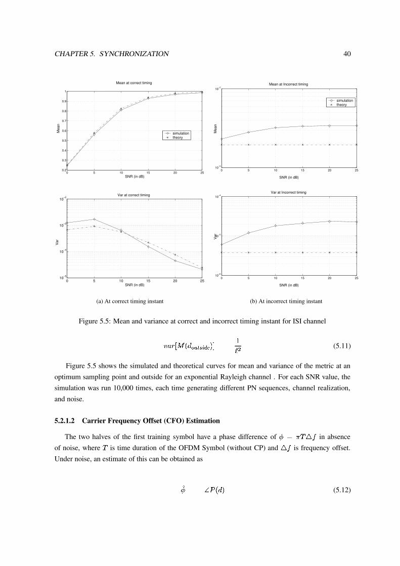
CHAPTER 5. SYNCHRONIZATION 40
0 5 10 15 20 250.2
0.3
0.4
0.5
0.6
0.7
0.8
0.9
1
SNR (in dB)
Mea
n
Mean at correct timing
simulationtheory
0 5 10 15 20 2510−5
10−4
10−3
10−2Var at correct timing
Var
SNR (in dB)
(a) At correct timing instant
0 5 10 15 20 2510−3
10−2
SNR (in dB)
Mea
n
Mean at Incorrect timing
simulationtheory
0 5 10 15 20 2510−6
10−5
10−4Var at Incorrect timing
Var
SNR (in dB)
(b) At incorrect timing instant
Figure 5.5: Mean and variance at correct and incorrect timing instant for ISI channel
a 6 � À l )�� ¨ b = ~ ; O K ,0Å z hA N (5.11)
Figure 5.5 shows the simulated and theoretical curves for mean and variance of the metric at an
optimum sampling point and outside for an exponential Rayleigh channel . For each SNR value, the
simulation was run 10,000 times, each time generating different PN sequences, channel realization,
and noise.
5.2.1.2 Carrier Frequency Offset (CFO) Estimation
The two halves of the first training symbol have a phase difference of: z � � XVY
in absence
of noise, where�
is time duration of the OFDM Symbol (without CP) andXZY
is frequency offset.
Under noise, an estimate of this can be obtained as
à: z Y w )���,(5.12)
CHAPTER 5. SYNCHRONIZATION 41
The fractional part of the frequency offset relative to the subcarrier spacing B±C'D�F39 can now be obtainedas
B3CED�FG9 z à:� (5.13)
The actual frequency offset is�ê/  N��/ where
�is some integer. By partially correcting the frequency
offset, adjacent carrier interference (ACI) can be avoided, and then the remaining offset¬ � § �
can be
found. After the two training symbols are frequency corrected byà: § ) � � ,
, let their FFT’s be£ 4 ! ¥ and£ N ! ¥ , where
£ ; ! ÷ corresponds to the retrieved data for <�=?> symbol andþ =?> subcarrier. An integer shift
in relative frequency will be reflected as a shift in data. Define Z as the set of indices for the even
frequency components, Z ={ � ¢ , � ¢ Â ¬,³E³E³
, � K � ¬ K ¬ K KE³E³E³JK ¢ ,¢ � ¬ , ¢ } where
¢ z½S § ¬. The
number of even positions shifted can be calculated by findingàp
to maximize
o )qpr, z 333 ç ¥�[]\ £ 14 ! ¥ ò N Ç a 1¥ £ N ! ¥ ò N Ç 333 N¬ ) ç ¥�[]\ û £ N ! ¥ û N , N (5.14)
where a ¥ z 0 N ~ ¹_^ �~`9 ^ � with ² ; ! ÷ corresponding to the actual data onþ =?> subcarrier of < =?> training symbol.
The frequency offset estimate then becomes
a XZY z à:� � Â ¬ àp� (5.15)
Variance of fractional estimate [24][28], for usable SNR values and sufficiently large value ofA,
is given by
a 6 � À à:� Å Ê h� N A � S ( (5.16)
This is indeed CRLB (Cramer Rao Lower Bound) which is not very surprising as the method for
fractional frequency offset estimation is an ML estimate [24]. Now if the integer part estimation is
correct, the total variance will be just that of fractional part.
The distribution for the metrico )qp�,
is Gaussian [22] with mean and variance given by
¦ À o )qp 9 ¨ D�D�K 9 = ,0Å z L /~)�L N~  L N` , N z � S ( N) � S ( ½h , N (5.17)
a 6 � À o )qp 9 ¨ D�D�K+9 = ,0Å z L /~ À ) h# ¬ Icb�,+L&N~ L&N`  ) h" Icb�,+L /` Å¢ )�L N~  L N` , / (5.18)

CHAPTER 5. SYNCHRONIZATION 42
0 5 10 15 20 2510−7
10−6
10−5
10−4
10−3
SNR (in dB)
Err
or V
aria
nce
theorysimulation
Figure 5.6: Performance of frequency offset estimator (fractional + integer part) for an exponentialRayleigh channel with N=1024
While at incorrect frequency offset,o )qpr,
has chi-square distribution with 2 degrees of freedom
and mean and variance given by
¦ À o )qp ; ` 9 ¨ D�D�K 9 = ,0Å � h¢ (5.19)
a 6 � À o )qp 9 ¨ D�D�K 9 = ,0Å � h¢ N (5.20)
Finally performance of joint frequency offset estimator is shown in figure 5.6 forS
=1024, ex-
ponential Rayleigh channel and frequency offset 2.4 subcarrier spacing. For each SNR value, the
simulation was run 10,000 times, each time generating different PN sequences, channel realizations,
and noise.
5.2.2 Minn Zeng Bhargava (MZB) Algorithm
In SCA, the timing metric reaches a plateau which leads to some uncertainty as to where the start of
frame is. This causes large variance of timing estimate. To improve on this, following methods were
proposed in [23].
5.2.2.1 Sliding Window Method (Method A)
In calculation of the half-symbol energy ( )���, , all samples over one symbol period is used instead
of the second half symbol period. Next, instead of 90% points averaging, the timing metric is simply
CHAPTER 5. SYNCHRONIZATION 43
averaged over a window of length ofSÈÇ�Âèh
samples whereS©Ç
is length of cyclic prefix. Then thetiming metric is given by
l 4 )���, z hS�Ç#Âýh�µ¥'¶ 2 R�Ç l C )��  [ , (5.21)
where l C )���, can be calculated as
l C )��r, z û w )��r, û N( NC )���, (5.22)
( C )��r, z h¬R 2&4µ� ¶ � û � )��  e , û N (5.23)
andw )��r,
is given by equation 5.3. The symbol timing estimate is taken as the argument of maximum
of this metric, l 4 )���, .5.2.2.2 Training Symbol Method (Method B)
The samples of training symbol method (excluding CP) are designed to be of the form
� z À ded � d � d Å (5.24)
where A represents samples of lengthA 4 z½S § generated by
S § point IFFT and data modulated by
PN sequence such that sum of the corresponding data equals zero. Then the timing metric is given by
l N )��r, z û w N )���, û N( NN )���, (5.25)
where
w N )���, z 4µ¥E¶ � N 9 2&4µ� ¶ � � 1 )��  ¬ [ A 4  e ,®* � )��  ¬ [ A 4  e  A 4 , (5.26)
( N )���, z 4µ¥E¶ � N 9 2&4µ� ¶ � û � )��  ¬ [ A 4  e  A 4 , û N (5.27)
In both methodsw N )��r, and ( N )��r, , or
w )���,and ( C )���, can be calculated iteratively as in case
of SCA. The timing metric of SCA and MZB are shown in figure 5.7 under no noise and distortion

CHAPTER 5. SYNCHRONIZATION 44
−0.5 0 0.50
0.2
0.4
0.6
0.8
1
1.2
Timing Offset (OFDM Symbols)
Tim
ing
Met
ric
SCAMZB AMZB B
Figure 5.7: Timing Metric of SCA and MZB under no noise and distortion condition
condition with the system parameterSÃzËhE° ¬±
,SÈÇ z hE° ¬
.
5.2.2.3 Simulations and Discussion
Performance of timing offset estimators have been investigated for following five cases : -
1. SCA with 90% Averaging
2. SCA (as in 1) with ( )���, replaced by ( C )��r, .3. Method A
4. Method B
5. Method B with ( N )���, replaced with ( C )���,The system used 1024 subcarriers OFDM system with 1024 point FFT, 10% guard interval (102
samples), CFO of 12.4 subcarrier spacing, BPSK modulation. For each SNR value, the simulation
was run 10,000 times, each time generating different PN sequences, channels, and noise. Two channel
were considered (i)AWGN and (ii) ISI (Exponential Rayleigh) with channel order=16.
Figure 5.8 and 5.9 show the mean and variance of the timing offset in AWGN channel and ISI
channel resp. For AWGN, means of cases 1 and 2 are in middle of plateau while for other cases it is
about correct timing point. For ISI, they are slightly shifted to the right in time axis by some amount
depending on shape of timing metric and ISI channel. Note that if the timing estimate is desired to be
within guard interval, then the means of 3-5 cases can be shifted to left (in advanced) by appropriate
design amount.

CHAPTER 5. SYNCHRONIZATION 45
0 5 10 15 20 25−60
−50
−40
−30
−20
−10
0
10
SNR (in dB)
mea
n
SCA (using R(d))MZB ASCA (using Rf(d))MZB BMZB B with R2f
(a) Mean vs SNR
0 5 10 15 20 2510−4
10−3
10−2
10−1
100
101
102
103
SNR (in dB)
var
SCA (using R(d))MZB ASCA (using Rf(d))MZB BMZB B with R2f
(b) Variance vs SNR
Figure 5.8: mean and variance of SCA and MZB in AWGN
0 5 10 15 20 25−60
−50
−40
−30
−20
−10
0
10
SNR (in dB)
mea
n
SCA (using R(d))MZB ASCA (using Rf(d))MZB BMZB B with R2f
(a) Mean vs SNR
0 5 10 15 20 25100
101
102
103
SNR (in dB)
var
SCA (using R(d))MZB ASCA (using Rf(d))MZB BMZB B with R2f
(b) Variance vs SNR
Figure 5.9: mean and variance of SCA and MZB in ISI

CHAPTER 5. SYNCHRONIZATION 46
MZB method has significantly less variance than SCA because of absence of plateau in timingmetric. In AWGN channel, cases 1-2 show floor variance, but 3-5 do not. In ISI channel, all of them
have floor variance. Using ( C )���, instead of ( )���, gives better performance. Overall ’case 5’ has best
performance.

Chapter 6
Proposed Scheme : Tone based IFOestimation
This scheme is based on the fact that Integer Frequency offset (IFO) causes data to be cyclically
shifted. Noting this simple fact, if we send pure tone i.e. data on only one subcarrier of the training
symbol and detect the shift in the position of this impulse (in frequency domain), the required IFO
can be obtained.
At transmitter, the data modulating the subcarriers for IFO training symbol is
² ) [ , z f ´ S w ~ [ z [ �° [ îz [ � (6.1)
´ S w ~is required because of constraint that the average power per OFDM symbol is the same. Let�®) j ,
=IFFTü ² ) [ ,3ÿ , where
[ K j B À ° K S � h Å�³ Note�®) j ,
are transmitted symbols. Let�P) j 9 , be the cor-
responding continuous time signal and ¤ ) j 9 , be the received (continuous) signal (without noise and
channel distortion) after frequency offset ofXZY
at receiver, then
¤ ) j 9 , z �®) j 9 , � ÷ N�ê�g C = �and in discrete time domain the same equation can be written as
¤ ) j , z �®) j , �3÷ N�ê = g ¥ ë Rwhere
XV[ z g Ch Xji , is frequency offset (FO) normalized to subcarrier spacing}"~q�
. Taking FFT, we get
47

CHAPTER 6. PROPOSED SCHEME : TONE BASED IFO ESTIMATION 48
£ ) [ , z ² ) [ � XZ[ , ï [(6.2)
So from equations 6.1 and 6.2, we have
£ ) [ , z f ´ S w ~ [ z [ � Â XV[° [ îz [ � (6.3)
Thus argument corresponding to maximum of£ ) [ ,
will have sufficient information about frequency
offset. If size of FFT at the receiver is sufficiently large, then both the fractional part and the integer
part can be estimated jointly. Unfortunately, this will result in high computational complexity.
The timing synchronization and fractional frequency offset correction have to be necessarily per-
formed before IFO. Hence the same is assumed here. In fact, we show later that SCA can be used
in conjunction with IFO training symbol for timing synchronization and fractional frequency offset
correction. So we will concentrate on IFO estimation only. Assuming that fractional part of frequency
offset has been removed, we can estimate the integer frequency offset as follows
s ) [ , z û £ ) [ , û N (6.4)[ d� z 6 � p ü øæù±ú¥ s ) [ ,3ÿ(6.5)aXZ[ ; z [ d� � [ � (6.6)
whereaXZ[ ;
will be integer such that � [ � �lkXZ[ ; � S � [ � .6.1 Some Observations for Proposed Scheme
1. Fractional frequency part by SCA gives an estimate in range of- h
subcarriers. Therefore if we
are sending impulse on an even subcarrier, then only even subcarriers need to be searched.
2. Frequency Acquisition range, the range of integer frequency offsets that can be corrected, is) S � [ � , � [ � zýS subcarriers i.e. entire OFDM bandwidth.
3. To change the frequency acquisition span from � [ � � XV[ ; � S � [ to � [ �  p � XZ[ ; �S � [  p , construct new search vectors 4 ) [ , z s ) [ � pr,GK i.e. C 4 zÐÀ s )qpr,GK s )qp  ¬ ,GKE³E³E³ s ) S �¬ ,GK s ) ° , ³E³E³ s )qp � ¬ ,0Å . Thus for
XV[ ;to be in range [ � S § ¬ K S § ¬ ],
p z [ � Â�S § ¬. Note thatXV[ ; K [
andp
are all even when impulse is sent on even subcarrier.
4. It is evident from equation 6.6, that the scheme is independent of subcarrier on which an
impulse is sent.

CHAPTER 6. PROPOSED SCHEME : TONE BASED IFO ESTIMATION 49
5. Scheme is independent of timing errors if starting of frame is in plateau of length (CP-L).This is straight forward, noting that timing offset will cause phase rotation in frequency domain
and our metric (see equation 6.5) is independent of phase rotation.
6. The similarity between the proposed scheme and M-orthogonal signaling (specially FSK)
scheme should be noted where one transmits 1 out of M orthogonal signals. In that case the op-
timal detector is given by equations 6.4 and 6.5. In fact, this scheme is M-orthogonal signaling
used for IFO estimation with slight modification.
7. For timing synchronization and fractional frequency offset correction in SCA, two identical
halves in time domain are required. When impulse is sent on an even subcarrier, we get two
identical halves in time domain of one OFDM symbol, so that SCA algorithm can be used for
timing synchronization and fractional frequency offset estimation in conjunction with IFO train-ing symbol. So our earlier assumption that fractional frequency offset is already correctedfor proposed scheme is valid.
8. If impulse is sent on any of the odd frequencies then we get two out of phase halves in one
OFDM symbol which can be used for SCA with phase modification (multiplication by -1 to
latter half) and rest of discussion will be similar to the one for even frequency.
9. Total frequency offset can be given as in equation 5.15,a XZY z à:� � Â ¬ aXZ[ ;� (6.7)
6.2 Mathematical Analysis
6.2.1 Data Model 1 : AWGN Channel
Data modulating the subcarriers of the training symbol are
² ) [ , z f ´ S wP~ [ z [ �° [ îz [ � (6.8)
Note that° � [ � S � h and
° � j � S throughout the analysis unless specified otherwise. AfterIFFT stage at the transmitter, we have
�P) j , z h´ S ² ) [ � , � ÷ N�ê ¥nm = ë R ï j z½° KE³E³E³K S � h (6.9)
Let k ) j , be AWGN noise with i.i.d real and imaginary part, each having varianceL N` i.e

CHAPTER 6. PROPOSED SCHEME : TONE BASED IFO ESTIMATION 50
k ) j ,QP H ) ° KML N` , Â þ H ) ° KML N` , (6.10)
Hence signal power =4R ç R 2&4` ¶ � û �®) j , û N z w ~ , and Noise Power =
¬ LÒN` . Therefore
� S ( z w ~¬ L N` (6.11)
The received signal is
��) j , z �P) j ,  k ) j , (6.12)
After frequency offset (without loss of generality assume FO to be integer only), the received signal
is
¤ ) j , z ��) j , �3÷ N�ê = g ¥�o ë R (6.13)
Taking FFT of both sides, we get
£ ) [ , z ² ) [ � XZ[ ; , Â ¢ ) [ � XZ[ ; , [ z [ d� (6.14)
where¢ ) [ ,
is FFT of k ) j , . Noting that[ � z [�d� � XZ[ ; , we get
£ ) [ , z f ² ) [ � ,  ¢ ) [ � , [ z [�d�¢ 4 ) [ , [ îz [�d� (6.15)
where¢ 4 ) [ ,qp ¢ ) [ � XZ[ ; , . Since k ) j , are i.i.d Gaussian random variables,
¢ ) [ ,and
¢ 4 ) [ , are
also i.i.d with Gaussian distribution
¢ ) [ ,rP H ) ° KML N` , Â þ H ) ° KML N` , (6.16)
Therefore the distribution of£ ) [ ,
is given by
£ ) [ d� ,rP H )�s S w ~ KML N` , Â þ H ) ° KML N` , (6.17)£ ) [ ,QP H ) ° KML N` , Â þ H ) ° KML N` , [ îz [ d� (6.18)

CHAPTER 6. PROPOSED SCHEME : TONE BASED IFO ESTIMATION 51
Distribution of metric at correct offset (i.e.[ z [�d� ) :
At correct offset, the metrics ) [ ,
is given by
s ) [ d� , z 333 s S w ~ Â ¢ ) [ � , 333 N zut s S w ~ Â ¢ ) [ � ,wv t s S w ~ Â ¢ ) [ � ,wv 1(6.19)z S w ~ Â û ¢ ) [ � , û N Â s S w ~ À ¢ ) [ � , Â ¢ 1 ) [ � ,0Å(6.20)
For high SNR, second term in above equation can be neglected and noting that the third term is nothingbut
¬ ( � ü ¢ ) [ � ,3ÿ, we get
s ) [ d� , z S w ~ Â ¬ s S w ~ ( � ü ¢ ) [ � ,3ÿ(6.21)
Therefore
s ) [ d� ,QP H ) S w ~ K S w ~ L N` , z H ) S w ~ K ¬ S w N~� S ( , (6.22)
where equality results from equation 6.11.
Distribution at incorrect timing instant (any[ îz [�d� , :
At incorrect offset the metrics ) [ ,
will become
s ) [ ; ` 9 , z û ¢ 4 ) [ ; ` 9 , û N (6.23)
Therefores ) [ ; ` 9 , has central chi square distribution with 2 degrees of freedom with mean and vari-
ance given by
¦ À s ) [ ; ` 9 ,0Å z ¬ L N` (6.24)a 6 � À s ) [ ; ` 9 ,0Å z L N` (6.25)
Probability of Error (w��
) expression :
Byw��
, we mean the probability that our estimate is not equal to actual IFO i.e.w�� z w ) aXV[ ; îzXZ[ ; ,
. Error will occur if we detect peak on incorrect offset i.e.s ) [ d� , � s ) [ ,
for one or more[ îz [�d� . So it is easier first to find Probability of correct estimation (wy�
) which is given by

CHAPTER 6. PROPOSED SCHEME : TONE BASED IFO ESTIMATION 52
wy� z xzy� w � ) �{� s ) [ ,GK ï [ îz [ d� K [ < ² � a � f § � ,P*�|®) � ,®*«� �z xzy� À } 9 ] ¥ _ ) � ,0Å ¼ ¹ 2&4 *�|P) � ,P*«� � Y ¿ � 6 f ¤ [ îz [ d� (6.26)
z hs ¬�� L N9 xMy� } h � ��~ 2 �¹]� ¹+��c� ¼ ¹ 2&4 ��~ 2 � �w� ¼�� X � ¹� ¼�� X � ¹+�� *O� � (6.27)
wheres ) [ d� , is denoted by
�for convenience,
|®) � , z 4´ N�ê V ¹� � ��|P) ] 9 2�� ] 9 _�_ ¹N V ¹� ,= pdf of
�,L N9 z a 6 � ) � , z S w ~ L N` by equation 6.22,
} D = CDF of r and is given by} D ) � , z¯h � � ��|�� � 9N V ¹�"� . The i.i.d nature
ofs ) [ ,
(ï [
) is used to derive equation 6.26. The Probability of error is given by
w�� z h � wy� (6.28)
6.2.2 Data Model 2 : ISI Channel
Assume Exponential Rayleigh channel with tap coefficients having distribution
� ) ¾ ,�P H ) ° K ° ³��·L N> é ,  þ H ) ° K ° ³��·L N> é , ï ¾ z½° KE³E³E³K � (6.29)
Expressions for ² ) [ ,GK��®) j , , and k ) f , are same as for AWGN case (see equation 6.8, 6.9, 6.10).
However,��) f , in this case is given by
� ) j , z �®) j , 7 � ) j ,  k ) j , (6.30)� ) j , z h´ S ² ) [ � , � ) [ � ,  k ) j , ï j z½° KE³E³E³K S � h (6.31)
where� ) [ � , z ç R 2&4= ¶ � � ) j , � 2 ÷ N�ê ¥nm = . Equation 6.31 arises from equations 6.9 and 6.30, and definition
of� ) [ � ,
. Therefore
� S ( z w ~ ç Ñé ¶ � L N> é¬ L N` (6.32)
After frequency offset, we get
¤ ) j , z ��) j , � ÷ N�ê = g ¥�o ë R (6.33)

CHAPTER 6. PROPOSED SCHEME : TONE BASED IFO ESTIMATION 53
Taking FFT, we get
£ ) [ , z f ² ) [ � , � ) [ � ,  ¢ ) [ � , [ z [�d�¢ 4 ) [ , [ îz [�d� (6.34)
Distribution of metric at correct offset :
Since£ ) [rd� , is sum of independent Gaussian random variables, it is Gaussian distributed as
£ ) [ d� ,�P H ) ° K S w ~¬ ѵ é ¶ � L N> é  L N` ,  þ H ) ° K S w ~¬ ѵ é ¶ � L N> é  L N` , (6.35)
Let us denoteLÒN9 p R D XN ç Ñé ¶ � L&N> é Â L&N` for convenience. So
s ) [rd� , z û £ ) [�d� , û N will have central chi
square pdf with two degrees of freedom with mean and variance given by following equations
¦ À s ) [ d� ,0Å z ¬ L N9 (6.36)a 6 � À s ) [ d� ,0Å z L /9 (6.37)
Distribution of metric at incorrect offset :
At incorrect offset,s ) [ ; ` 9 , z û ¢ 4 ) [ , û N , so distribution of metric at incorrect offset is same as for
AWGN and mean and variance are given by equations 6.24 and 6.25.
Probability of error :
Probability of correct estimationw��
is same as for AWGN case (see equation 6.26) except that|®) � ,
in this case in central chi square instead of Gaussian in AWGN case i.e.
|®) � , z h¬ L N9 � �#|�� � �¬ L N9�� (6.38)
Therefore equation for probability of correct decision in this case is given by
w�� z h¬ L N9 x y� } h � � ~ 2 �¹]� ¹+ �c� ¼ ¹ 2&4 � ] 2 �¹]� ¹� _ *«� � (6.39)
and probability of error can be calculated asw�� z h � wy� (6.40)

CHAPTER 6. PROPOSED SCHEME : TONE BASED IFO ESTIMATION 54
SW�SNR �(in dB)
h«ª F ¬ ª h ¬��-4
h ³�� � TnhE° 2&4 F ³���� TihE° 2�N h ³���� TihE° 2�� F ³ hyTihE° 2��° h ³ ° ªæTihE° 2�N ¬ ³ °#�ÉTihE° 2 / � ³ F � TihE° 2�� F TnhE° 2&4 � h ³ ��h�TihE° 2 / � TihE° 2&4 � ªõTihE° 2&4�4 °� ª ³ �¬ TihE° 2�� ° ° °Table 6.1:
w��for various values of SNR and
Sin AWGN scenario (theoretical)S��
SNR �(in dB)
h«ª F ¬ ª h ¬��-4
h ³�� ¬ T hE° 2&4 ¬ ³ � ªÈTnhE° 2�N ��³�� TihE° 2 / � hE° 2��° ³ ° ªÉT hE° 2�N h TihE° 2�� � hE° 2�� � hE° 2�� � hE° 2�� � hE° 2�� � hE° 2�� � hE° 2��� � hE° 2�� � hE° 2�� � hE° 2�� � hE° 2��Table 6.2:
w��for various values of SNR and
Sin AWGN scenario (simulation)
6.3 Simulation Results and Observation
AWGN Channel :
Tables 6.1 and 6.2 presents the simulated and theoretical values forw��
for various values of
SNR andS
for AWGN channel. For each SNR value, the simulation was runhE° �
times, each time
generating different PN sequences, and noise. Cyclic prefix of 12 was used. BPSK modulation was
used. For every realization, the frequency offset as well as subcarrier index on which impulse was
sent, were changed. It can be seen that performance of the proposed tone based scheme is very good,
even in low SNR and lowS
. It decreases monotonically with increasing SNR and with increasingS. The simulation and theoretical results are slightly mismatching for low values of SNR, but this
can be explained by the fact that simplified theoretical expression (see equations 6.21 and 6.28) were
obtained for high SNR values and the values obtained in tables are for low SNR. For High SNR values,they are approximately same.
ISI Channel :
Figure 6.1 shows (a)w��
Vs SNR and (b)w��
VsS
curves for Exponential decaying Rayleigh Chan-
nel (ISI) for simulation and theoretical cases. For each SNR value, the simulation was runhE° �
times,
each time generating different PN sequences, channel realizations, and noise. Channel Order was�
=5.
Channel tap coefficients were normalized so that sum of variances of each tap was 1 i.e.ç Ñé ¶ � L N> é z h .
Cyclic Prefix length was 12. BPSK modulation was used. It can be seen that the simulation and theo-

CHAPTER 6. PROPOSED SCHEME : TONE BASED IFO ESTIMATION 55
0 5 10 15 20 2510−5
10−4
10−3
10−2
10−1
SNR (in dB)
Pe
simulation N=64theory N=64simulation N=512theory N=512
(a) Pe Vs SNR
0 200 400 600 800 1000 120010−5
10−4
10−3
10−2
10−1
N
Pe
simulation SNR=5theory SNR=5simulation SNR=20theory SNR=20
(b) Pe Vs N
Figure 6.1:w��
curves for Exponential Rayleigh (ISI) channel
retical values from mathematical analysis are approximately same. The performance of the proposed
tone based scheme is good in high SNR and highS
. It decreases monotonically with increasing SNR
and with increasingS
. The performance of scheme has deteriorated as compared to its performance
in AWGN, for which some modification has been proposed to improve the performance of this scheme
in ISI conditions.
Effect of timing offset :
Figure 6.2 show thew��
curves for different timing offset (TO). Here ’0’ corresponds to exact start
of data part in the training symbol. It can be seen that for TO between (-(CP-�
) to 0 i.e. -6 to 0 in this
case) has loww��
as compared to other offsets andw��
value is approximately same in this region.
6.4 Modification to the Proposed Scheme for ISI case (Multitone)
Whenever channel at subcarrier[ �
is bad i.e.� ) [ � ,
has small value, then the proposed tonebased algorithm performs rather badly. To improve on this, we shall send data on more number of
subcarriers in IFO training symbol, giving frequency diversity and hence a good performance. We will
henceforth use notation� e to denote case of Multitone scheme, in which data is sent on e subcarriers
of IFO training symbol and rest of subcarriers will carry zeroes. The mathematical analysis has been
performed for� e . The cost to be paid is the frequency acquisition range is reduced by e . To get
optimum frequency acquisition the subcarrier have to be kept equidistant from each other.

CHAPTER 6. PROPOSED SCHEME : TONE BASED IFO ESTIMATION 56
−25 −20 −15 −10 −5 0 5 10 1510−4
10−3
10−2
10−1
TO (in Time/Ts)
Pe
SNR=0 dBSNR=20 dB
Figure 6.2:w��
vs Timing Offset
6.4.1 Mathematical Analysis
Data modulating the subcarriers of the IFO training symbol are
² ) [ , z ��¡ £¢ R D X� [ z [ ;° [ îz [ ; (6.41)
where[ ;
denote the subcarrier index on which data i.e. ( ¢ R D X� ) is send in IFO training symbol, and
it is given by[ ; z [ � Â ; R� and < zý° K h KE³E³E³K eó� h . Following the similar argument as in case of ISI
for tone based scheme, at receiver we get
£ ) [ , z f ² ) [ ; , � ) [ ; , Â ¢ ) [ ; , [ z [�d;¢ 4 ) [ , [ îz [�d; (6.42)
Metric is same as given by equation 6.4 i.e. begin_inset Formula $C(k)=, but nowaXZ[ ;
is given as
[ � Fn¤ z 6 � p ü øÉù±ú¥ s ) [ ,3ÿkXZ[ ; z ) [ � F`¤ � [ � , e ¿ � ) S § e , (6.43)

CHAPTER 6. PROPOSED SCHEME : TONE BASED IFO ESTIMATION 57
Distribution of metric at correct offset :
Distribution of£ ) [ ,
at correct offset can be obtained in similar way to ISI case for� h
and is given
by
£ ) [ d� ,�P H ) ° K S w ~¬ e ѵ é ¶ � L N> é% L N` ,  þ H ) ° K S w ~¬ e ѵ é ¶ � L N> é% L N` , (6.44)
For convenience, denoteL N9 � p R D XN � ç Ñé ¶ � L N> é Â L N` ³ Then
s ) [ d� , z û £ ) [ d� , û N will have a central chi
square pdf with two degrees of freedom with mean and variance given by following equations
¦ À s ) [ d� ,0Å z ¬ L N9 � (6.45)a 6 � À s ) [ d� ,0Å z L /9 � (6.46)
Distribution of metric at incorrect offset :
At incorrect offset,s ) [ ; ` 9 , z û ¢ 4 ) [ , û N , so distribution of metric at incorrect offset is same as for
AWGN and mean and variance are given by equations 6.24 and 6.25.
Probability of error :
Probability that metric at correct offset[ ;
(for < z½° K h KE³E³E³±K e � h ) is greater than metric values at
all incorrect offset (there areR N �Íe such offsets) is similar to equation 6.39 and is given by
wy�$; z h¬ L N9 � x y� } h � � ~ 2 � o¹]� ¹+ � � ¼ ¹ 2 � � ] 2 � o¹]� ¹��¥ _ *«� �$; < z ° K h KE³E³E³K e � hwhere
�$; p s ) [ d; , for convenience. Therefore Probability that metric at correct offset[ ;
is less than
metric value at one or more of the incorrect offsets, will be given by
w��E; z h � wy�$; < z ° K h KE³E³E³±K e � hNow our estimation of IFO will go into error only if both
s ) [ ; ,for < z ° K h KE³E³E³K e � h are less than
somes ) [ , [ îz [ ;
. Therefore probability of error for� e will be given byw�� ~�� z w�� � * w�� 4 *�³E³E³%* w�� � 2&4 z ) w�� � , � � < ³ < ³ � (6.47)
Now it has been observed numerically that for various SNR values

CHAPTER 6. PROPOSED SCHEME : TONE BASED IFO ESTIMATION 58
w�� ~ 4 � w�� � � e w�� ~ 4 (6.48)
wherew�� ~ 4 is probability of error for
� hand is given by equation 6.40. The first inequality is logical,
since now strength of impulse has reduced by factor of e (for� e ) as compared to
� h. As SNR
increasesw��O�
moves toward upperbound. From equations 6.47 and 6.48, we get upperbound onw�� ~��, which is given by
w��O~0� � ) e w��~ 4 , � (6.49)
Solving forw�� ~0� � ) e w�� ~ 4 , � � w�� ~ 4 we will get the values of
w�� ~ 4 , for which scheme will
perform better for� e as compared to
� h. The expression for required
w�� ~ 4 is
w�� ~ 4 � e * � ��|P) eh � e , (6.50)
which turns out to bew�� ~ 4 � h
for values of e � F . Sincew��
cannot be greater than 1, the
performance will be better for everyw�� ~ 4 (even for e z
). For e z ¬,w�� ~ 4 � ° ³ ¬ � and for e z ¬w�� ~ 4 � ° ³ ª � which is true even for low
Sand low SNR.
6.4.2 Simulation Results and Observation
Figure 6.3 shows simulation results for� h
,��¬
and�P
. Simulation parameters were similar to� h
,
except that IFO here was limited to the new acquisition range. For each SNR value, the simulation was
runhE° �
times, each time generating different PN sequences, channel realizations, and noise. It can be
seen that performance has greatly improved. Performance of Multitone scheme goes on improving ase increases but the acquisition range is reduced by the same factor. Hence there is trade off between
acquisition range andw��
. In general, e z should be sufficient as it gives good performance at low
SNR and lowS
and acquisition range is one-fourth of OFDM bandwidth.
6.5 Comparison between the proposed schemes and existing schemes
Multitone is general case. For comparison with existing scheme it is used (except for performance
in AWGN scenario where Single tone is sufficient).

CHAPTER 6. PROPOSED SCHEME : TONE BASED IFO ESTIMATION 59
0 5 10 15 20 2510−5
10−4
10−3
10−2
10−1
100
SNR
Pe
S1 N=16S2 N=16S4 N=16
(a) Pe vs SNR
0 50 100 150 200 250 30010−5
10−4
10−3
10−2
10−1
100
NP
e
S1 SNR=0 dBS2 SNR=0 dBS4 SNR=0 dB
(b) Pe Vs N
Figure 6.3: Comparison of Multitone scheme for� h
,��¬
, and�®
−4 −2 0 2 4 6 8 10 1210−3
10−2
10−1
100
SNR (in dB)
Pe
Proposed N=16SCA N=16
(a) Pe Vs SNR
0 50 100 150 200 250 30010−4
10−3
10−2
10−1
100
N
Pe
Proposed SNR=−4dBSCA SNR=−4dB
(b) Pe vs N
Figure 6.4:w��
Curves for Tone based scheme and SCA for different values of SNR andS
in AWGNconditions

CHAPTER 6. PROPOSED SCHEME : TONE BASED IFO ESTIMATION 60
0 5 10 15 20 2510−5
10−4
10−3
10−2
10−1
SNR (in dB)
Pe
S1S2S4SCA
(a) Pe vs SNR (for N=32)
0 50 100 150 200 250 30010−5
10−4
10−3
10−2
10−1
100
N
Pe
S1 S2S4SCA
(b) Pe vs N (for SNR =0 dB)
Figure 6.5:w��
Curves for Multitone scheme and SCA for different values of SNR and N for expo-nential decaying Rayleigh channel
6.5.1 Performance
AWGN Case :
Figure 6.4 showsw��
curves for the proposed scheme and SCA frequency offset estimation for AWGN
scenario. Simulation parameters were similar to� h
, except that IFO here was kept limited to the new
acquisition range. For each SNR value, the simulation was runhE° �
times, each time generating
different PN sequences, channels, and noise. Subcarrier Index on which impulse was sent, was kept
changing in allowed range° � [ � � S , and
[ �is even. It was seen that performance of proposed
scheme (� h
) is better than that of SCA.
ISI Case
Figure 6.5 shows thew��
curves for the Multitone scheme and SCA frequency offset estimation
for ISI scenario. Except for the channel model, simulation scenario is similar to that for AWGN case
mentioned above. It was observed that for high SNR and highS
, the performance of SCA is better
than� h
and��¬
, but the performance is comparable with�®
.
From the above figure, we don’t get much idea about comparison of SCA and Multitone scheme
with�®
at highS
and SNR. For these values ofS
and SNR,w��
values are very low. Simulating for
such condition involves enormous computation complexity. So we tried to analytically compare them
on basis of theirw��
equations.w��
equation for SCA IFO is similar to proposed tone based scheme for
AWGN case (see equations 6.27 and 6.28) except that distributions at correct offset will be now givenby equations 5.17,5.18 and distribution at incorrect offset will now be given by equations 5.19 and

CHAPTER 6. PROPOSED SCHEME : TONE BASED IFO ESTIMATION 61
0 5 10 15 20 2510−12
10−10
10−8
10−6
10−4
10−2
100
SNR (in dB)
Pe
S4SCA
(a) Pe vs SNR for N=32
15 20 25 30 35 40 45 50 55 60 6510−9
10−8
10−7
10−6
10−5
10−4
10−3
10−2
10−1
N
Pe
S4SCA
(b) Pe vs N for SNR=10 dB
Figure 6.6: Theoreticalw��
curves for SCA and Multitone scheme�®
Operation SCA Proposedcomplex multiplication
° ³��y* S N  S–
complex divisionS § ¬
(for a [ ) –complex addition
S N § ¬–
real divisionh h
(mod operation)
Table 6.3: Relative Computation Complexity for SCA and Proposed Scheme
5.20. So numericallyw��
values where obtained for SCA and�®
. Values ofw��
for�®
is calculated
from equation 6.47. The corresponding plots are shown in figure 6.6. One thing worth noting from
these plots is thatw��
decreases exponentially with increase in SNR (dB) in case of Multitone scheme
but same is not true in case of SCA (even though there is monotonic decrease, but the rate is slow).
On other handw��
decreases exponentially with increasingS
in case of SCA and the rate of decrease
is low in case of Multitone scheme with increase inS
.
6.5.2 Computation Complexity
We have calculated the computational complexity for SCA IFO estimation from equation 5.14.
Similarly for the Multitone scheme (which is general case), computational complexity is calculated
from equation 6.4. Table 6.3 summarizes relative computational complexities between SCA and pro-
posed scheme for IFO estimation. By relative computation complexity we mean that the computations
common to both have been ignored (calculatingS § ¬
absolute square quantities). It can be seen that
the proposed scheme has very low complexity.

CHAPTER 6. PROPOSED SCHEME : TONE BASED IFO ESTIMATION 62
6.5.3 Frequency Acquisition Range
The Frequency Acquisition range for SCA is total OFDM bandwidth, and in case of Multitone
scheme the range is total bandwidth divided by e . But for small values of e zmhtohǻ
, it is still
a big range because most standards have frequency offset of at most few subcarrier spacings. For
802.11a WLAN standard, maximum frequency offset is 50 ppm at 5 GHz carrier frequency and 250
KHz subcarrier spacing. For this values, maximum frequency offset turns out to be 250 KHz i.e. one
subcarrier spacing.
6.5.4 Number of Training symbol required
Case I. For Multitone scheme, no additional symbol is required for timing synchronization and frac-
tional frequency offset estimation. But we will require an additional symbol for channel estimation.
Case II. We can perform timing synchronization and fractional frequency offset estimation using
first of the two SCA training symbols. For the second training symbol, if we put data on odd subcar-
riers, we can apply proposed scheme on even subcarriers. The channel estimation can be carried out
using even subcarriers of first training symbol and odd subcarriers of second training symbol.
Hence in both cases, we require at least 2 training symbols for timing synchronization, frequency
offset correction and channel estimation.
6.6 Performance of Multitone scheme for timing synchronization andfractional frequency offset
This section aims at evaluating the performance of timing synchronization and fractional frequency
offset estimation using SCA in conjunction with IFO training symbol (Case I of section 6.5.4). Sim-
ulations have been performed forS zghE° ¬±
in AWGN case to check whether the performance of
the the proposed training symbol will work accurately. Figure 6.7 shows mean and variance at cor-
rect timing region (point inside plateau). Figure 6.8 shows mean and variance at instant outside the
plateau. Figure 6.9 shows variance of error in estimating fractional frequency offset. From all these
figures, it can be concluded that the SCA work satisfactorily for IFO training symbol, in respect of
timing synchronization and fractional frequency offset estimation.

CHAPTER 6. PROPOSED SCHEME : TONE BASED IFO ESTIMATION 63
0 5 10 15 20 250.2
0.3
0.4
0.5
0.6
0.7
0.8
0.9
1
SNR (in dB)
Mea
n simulationthoery
0 5 10 15 20 2510−8
10−7
10−6
10−5
10−4
10−3
Var
SNR (in dB)
simulationthoery
(a) at correct instant
0 5 10 15 20 25
0.5
1
1.5
2
2.5
3x 10⁻³
SNR (in dB)
Mea
n
simulationtheory
0 5 10 15 20 251
1.5
2
2.5
3
3.5
4
4.5
5
5.5
6x 10⁻⁶
Var
SNR (in dB)
simulationthoery
(b) At incorrect instant
Figure 6.7: Mean and Variance at correct and incorrect timing instant forSÃzËhE° ¬±
and AWGN case,e z .

CHAPTER 6. PROPOSED SCHEME : TONE BASED IFO ESTIMATION 64
0 5 10 15 20 25−60
−50
−40
−30
−20
−10
0
10
SNR
mea
n
MZB ASCA 90%
(a) mean vs SNR
0 5 10 15 20 2510−2
10−1
100
101
102
103
SNR
var
MZB ASCA 90%
(b) Var vs SNR
Figure 6.8: mean and variance at correct timing instant
0 5 10 15 20 2510−7
10−6
10−5
10−4
10−3
SNR (in dB)
var o
f err
or
simulationtheory
Figure 6.9: Variance of Fractional FO error

Chapter 7
Conclusions
In the early part of this work, dependency of PAPR on input constellation (through 8 9 ) was derived
and corresponding expression forw �
was obtained for general constellations. Using this it was shown
that PAPR for QAM is more than that for PSK of any order. A Pulse shaping scheme for PAPRreduction was also proposed. An analytical expression for reduction in upperbound on PAPR was
obtained for the same.
In subsequent part, IOFDM was reviewed from PAPR reduction point of view for constant code
rate. IOFDM was shown to be Superset of OFDM and SC-FDE. Trade-off can be achieved OFDM
and SC-FDE by changing P (interleaving factor of IOFDM). BOFDM was proposed (structure sim-
ilar to IOFDM but without interleaving and minor differences). It was shown that BOFDM is also
superset of OFDM and SC-FDE. Later it was shown that BOFDM has more complexity than IOFDM.
Performances of SLM, PTS, and IOFDM were compared and it was found that IOFDM is better than
the other two schemes with respect to complexity, PAPR reduction, and amount of redundancy added.
Two Synchronization algorithms (1) SCA and (2) MZB were studied and implemented and a new
scheme was proposed for IFO estimation which is simple and highly computationally efficient as
compared to the existing schemes. A detailed mathematical analysis was carried out and Probability
of error (w��
) expression for ISI and AWGN channel was derived. A modification (Multitone) was
suggested which greatly improves the performance of the scheme even in lowS
and low SNR con-
dition for ISI channel, but at the cost of reduced frequency acquisition range. General expressionw��~��, i.e. Probability of error for
� e was also derived. An upperbound has been obtained onw���~0�
in terms ofw�� ~ 4 . The expression for range of values of
w�� ~ 4 for whichw�� ~��
will be less thanw�� ~ 4
(performance of e subcarrier case was better than 1 subcarrier case), is obtained. It was observed that
for e � F , the performance of� e case will be better than that of
� hcase.
Future Directions
In case of input stream consisting of binary sequences of different probabilities, PAPR can be
reduced by assigning sequences with low probabilities to symbols in constellation with high power.
65

CHAPTER 7. CONCLUSIONS 66
This will shift the CCDF curves for PAPR to left. But the probability assignment does not seem tobe trivial. It changes average power of constellation resulting in change in upper bound on
w ;. So
optimum allocation of sequences to the constellation symbols according to their probabilities is open
problem.

Bibliography
[1] Z.Wang and G.B.Giannakis, Wireless multicarrier Communications : Where Fourier meets Shan-
non IEEE SP magazine 2001.
[2] R.van Nee and Ramjee Prasad, OFDM for Wireless Multimedia Communication, Norwood,
MA:Archtech House,2000.
[3] J.G.Proakis, D.G.Manolakis, Digital Signal Processing, Prentice Hall 1997.
[4] J.G.Proakis, Digital Communication, McGraw Hill 2001.
[5] V.G.S.Prasad, Multiple Input Multiple Output techniques for Interleaved Orthogonal Frequency
Division Multiplexing, Masters Thesis, Department of Electrical Communication Engineering,
Indian Institute of Science, January 2002.
[6] V.G.S.Prasad, K.V.S.Hari, Interleaved Orthogonal Frequency Division Multiplexing (IOFDM)
system , IEEE Transaction on Signal Processing, Vol No.52, No.6, June 2004.
[7] Karthik Subramaniam, Alternative Interleaving Schemes for Interleaved Orthogonal Frequency
Division Multiplexing, MSc Thesis, Department of Electrical Communication Engineering, Indian
Institute of Science, August 2003.
[8] L.Litwin, M.Pugal, The Principles of OFDM, RF Signal Processing, January 2001.
[9] J.H.Manton, Dissecting OFDM : The Independent Roles of the Cyclic Prefix and IDFT operation,
IEEE Communication Letters, Vol.5, No.12, December 2001.
[10] G.B.Giannakis, P.Duhamel, Z.Wang, Cyclic Prefixing Or Zero-Padding for Wireless Multicar-
rier Communication?, IEEE Transaction on communications, August 2001.
[11] C.Tellumbura, Upper Bound on Peak Factor of N carriers system , Electronics Letters, Vol no.33,
No.19, September 1997.
[12] C.Tellumbura, Phase optimization criterion for reducing Peak to Average Ratio in OFDM, Elec-
tronic Letters vol. no.34, no.2, January 1998.
67

BIBLIOGRAPHY 68
[13] S.H.Muller, J.B.Huber, OFDM with reduced peak to power ratio by optimum combination of
partial transmit sequences, Electronic Letters vol.33, No.5, February 1997.
[14] R.Buaml, J.Huber, Reducing the Peak to Average Power Ratio of multicarrier modulation by
Selected Mapping, Electronic Letters Vol 32, No.22, October 1996.
[15] S.H.Muller, J.B.Huber, A Comparison of Peak Power Reduction Sequences for OFDM , Global
Telecommunications Conference, 1997. GLOBECOM ’97., IEEE ,Volume: 1 , 3-8 Nov. 1997
[16] A.D.S.Jayalath, C.Tellambura, The use of Interleaving to reduce the Peak to Average Power
Ratio of an OFDM signal , Global Telecommunications Conference, 2000. GLOBECOM ’00.
IEEE ,Volume: 3 , 27 Nov.-1 Dec. 2000
[17] S.B.Slimane, Peak to Average Power ratio reduction by Pulse Shaping. Global Telecommunica-
tions Conference, 2000. GLOBECOM ’00. IEEE ,Volume: 3 , 27 Nov.-1 Dec. 2000
[18] D.Falconer, B.Eidson, Frequency Domain Equalization for Single Carrier Broadband Wireless
Systems, IEEE Communication Magazine, April 2002.
[19] H.Sari, G.Karam, J.Jeanclaude, Transmission Technique for digital terrestrial TV broadcasting,
IEEE Communication Magazine 1995.
[20] M.J.E.Golay, Golay complementary series, IRE Transactions on Information Theory , Vol.IT-7,
April 1961.
[21] J.Jedwab, J.A.David, Peak to mean power control in OFDM, Golay complementary sequences,
and Reed Muller codes, IEEE Transactions on Information Theory, Vol.45. No.7, November 1999.
[22] T.M.Schmidl, D.C.Cox, Robust Frequency and Timing Synchronization for OFDM , IEEE Trans.
Commun., vol 45, pp 1613-1621 Dec 1997.
[23] H.Minn, M.Zeng, V.K.Bhargava, On Timing Offset Estimation for OFDM Systems, IEEE Com-
munication Letters, Vol 4, No.7, July 2000.
[24] P.H.Moose A Technique for Orthogonal Frequency Division Multiplexing frequency offset cor-
rection, IEEE Trans. on Commun., Vol 42. No.10, pp 2908-2914, Oct 1994.
[25] Jian Li, G.Liu, G.B.Giannakis, Carrier Frequency Offset Estimation for OFDM based WLANs.
IEEE Signal Processing Letters, Vol 8, No.3, pp 80-82, March 2001.
[26] Kalyan.K.G, Synchronization Algorithms for OFDM based Systems, Masters Thesis, Department
of Electrical Communication, Indian Institute of Science, Jan 2003.
[27] H.Koyabashi, A Novel Symbol Frame and Carrier Frequency Synchronization for Burst Mode
OFDM Signal. VTC-2000.

BIBLIOGRAPHY 69
[28] D.Rife and R.Boorstyn, Single Tone Parameter Estimation from discrete time observation, IEEETrans. Inform. Theory, Vol. IT-20, pp 591-598, Sept. 1974.