FEDERAL RESERVE BANK OF SAN FRANCISCO

WORKING PAPER SERIES

Pegged Exchange Rate Regimes – A Trap?

Joshua Aizenman University of California, Santa Cruz

and

Reuven Glick

Federal Reserve Bank of San Francisco

September 2005

Working Paper 2006-07 http://www.frbsf.org/publications/economics/papers/2006/wp06-07bk.pdf

The views in this paper are solely the responsibility of the authors and should not be interpreted as reflecting the views of the Federal Reserve Bank of San Francisco or the Board of Governors of the Federal Reserve System. This paper was produced under the auspices for the Center for Pacific Basin Studies within the Economic Research Department of the Federal Reserve Bank of San Francisco.

Pegged Exchange Rate Regimes – A Trap?*

Joshua Aizenman and Reuven Glick

September, 2005

Abstract: This paper studies the empirical and theoretical association between the duration of a pegged exchange rate and the cost experienced upon exiting the regime. We confirm empirically that exits from pegged exchange rate regimes during the past two decades have often been accompanied by crises, the cost of which increases with the duration of the peg before the crisis. We explain these observations in a framework in which the exchange rate peg is used as a commitment mechanism to achieve inflation stability, but multiple equilibria are possible. We show that there are ex ante large gains from choosing a more conservative not only in order to mitigate the inflation bias from the well-known time inconsistency problem, but also to steer the economy away from the high inflation equilibria. These gains, however, come at a cost in the form of the monetary authority’s lesser responsiveness to output shocks. In these circumstances, using a pegged exchange rate as an anti-inflation commitment device can create a “trap” whereby the regime initially confers gains in anti-inflation credibility, but ultimately results in an exit occasioned by a big enough adverse real shock that creates large welfare losses to the economy. We also show that the more conservative is the regime in place and the larger is the cost of regime change, the longer will be the average spell of the fixed exchange rate regime, and the greater the output contraction at the time of a regime change.

Joshua Aizenman Reuven Glick Department of Economics Economic Research Department University of California, Santa Cruz Federal Reserve Bank of San Francisco jaizen@ucsc.edu reuven.glick@sf.frb.org

JEL Classification: F15, F31, F43 Keywords: Pegged exchange rate, duration, crises, credibility, discretion, monetary regime change

*We thank Jessica Wesley for research assistance. The views presented in this paper are those of the authors alone and do not necessarily reflect those of the NBER, the Federal Reserve Bank of San Francisco or the Board of Governors of the Federal Reserve System.

2

1. Introduction

Exits from pegged exchange rate regimes have often been accompanied by crises and

severe declines in economic activity. Major currency crises over the past decade have had

particularly adverse effects on output growth; for example, output declined by 6% in Mexico

in 1995, 7% in Thailand and Korea in 1998, and by more than 11% in Argentina in 2002.

Eichengreen (1999), documenting the absence of an exit strategy from fixed exchange rates for

many countries, concludes: “…exits from pegged exchange rates have not occurred under

favorable circumstances. They have not had happy results.”

This paper provides an explanation for why pegged exchange rate regimes have tended

to end so explosively. It argues that using pegged exchange rate as a commitment device for

achieving inflation stability can create a “trap” whereby the regime initially confers gains in

anti-inflation credibility, but ultimately results in an exit occasioned by large adverse real

shocks, resulting in big welfare losses to the economy. We thus suggest that fixed exchange

rate regimes can plant the seeds of their own demise.

We do so in a framework extending Obstfeld (1996)’s setting, where the monetary

authority determines the exchange rate (and hence the inflation rate) based on its the degree of

aversion to inflation relative to output fluctuations, the magnitude of shocks, and the (fixed)

cost of allowing discrete exchange rate changes. Specifically, we assume that the monetary

authority is chosen from a pool of possible candidates/regimes, each differing in its degree of

anti-inflation firmness.

In accordance with Rogoff (1985)’s insight, we find that the optimal monetary

authority candidate is characterized by a “conservative bias”, i.e. a relative weight on inflation

stabilization greater than that of society as a whole, in order to mitigate the inflation bias

arising from time inconsistency. However, in our framework we also show that multiple

equilibria are possible. In this case there are ex ante gains from choosing a more conservative

monetary authority not only in order to lower private sector inflation expectations and mitigate

the inflation bias, but also to steer the economy away from high inflation equilibria. These

gains, however, come at a cost in the form of the monetary authority’s lesser responsiveness to

output shocks. Hence in choosing the monetary authority there is a tradeoff between, on the

3

one hand, the gains from greater firmness in stabilizing inflation and, on the other hand, the ex

post costs associated with a lesser willingness to respond to real shocks to the economy.

This tradeoff may plant the seeds of the regime’s ultimate demise: bad enough shocks

ultimately lead to the costly collapse of the regime. This result follows from the observation

that large negative output shocks not resulting in devaluation will induce welfare losses to the

public. In these circumstances, the gap in welfare evaluation between the public and monetary

authority is of a first-order magnitude, proportional to the difference between the public’s and

the monetary authority’s degree of firmness. Ultimately, for a bad enough shock, the cost of

sustaining the existing regime will rise above the cost of regime change, inducing a large

devaluation accompanied by sizable disruption of the economy. This suggests that more

conservative and longer-lasting pegged regimes are likely to end with severe output losses.

That is, the longer the duration of a peg before its collapse, the greater is the adverse effect on

the economy when it does collapse.1

These results may explain the severity of the demise of an Argentinean type of

currency board: legally anchoring the currency board in the constitution increased the cost of

devaluation and regime change, but also planted the seeds of a trap associated with the fixed

exchange rate regime. While in the short run it led to obvious credibility gains, it also

increased the duration of the peg as well as the output costs associated with the devaluation

that occurred when Argentina ultimately exited from the regime.

There is a vast literature on why pegged regimes may be crisis prone, dealing with

issues that are well beyond the scope of the present paper. Some focus on how limiting

exchange rate flexibility may increase risk taking by borrowers and lenders. Others focus on

how liberalization and increased capital mobility have increased exposure to shocks,

particularly those creating inconsistencies between a currency peg and other macroeconomic

policies (see Agenor and Montiel (1999) and Obstfeld and Rogoff (1996) for further details).

Our study is more closely related to papers that have studied the impact of policy maker

preferences on the conduct of discretionary policy (see Cukierman and Liviatan (1991),

Lohman (1992), and the references therein).

1 Klein and Marion (1997) analyze the duration of exchange rate regimes in Latin America. Husain, Mody and Rogoff (2005) study exchange rate regime durability and performance in developing versus advanced economies.

4

Section 2 presents some stylized facts about the severity of output declines during

recent exits from pegged regimes. In section 3 the theoretical model is presented. Section 4

concludes.

2. Simple Stylized Facts about Exits

To examine the decline in economic activity associated with exits to more flexible

exchange rate regimes we make use of the data set assembled by Detragiache, Mody, and Okada

(2005). They identify 63 episodes over the period 1980-2001 in which countries with heavily

managed exchange rates ended in an exit, defined as a move to a more flexible exchange rate

regime.2 Of these 63 episodes, 32 are deemed “disorderly” in the sense that currency fell freely at

some time during the 12 month period after the exit; the remaining episodes are deemed

“orderly”.

The top panel of Figure 1 presents event windows for the full sample of episodes

showing the average behavior of real GDP growth for the years before, during, and after exits

from pegged regimes, with the observations surrounded by two standard deviation bands.3 The

figure shows that economic growth typically slows in the periods leading up the exit, is almost

zero on average in the year after the exit occurs, following which growth recovers. For the

subsample of disorderly exits in the bottom panel, the depth of the downturn is more severe and

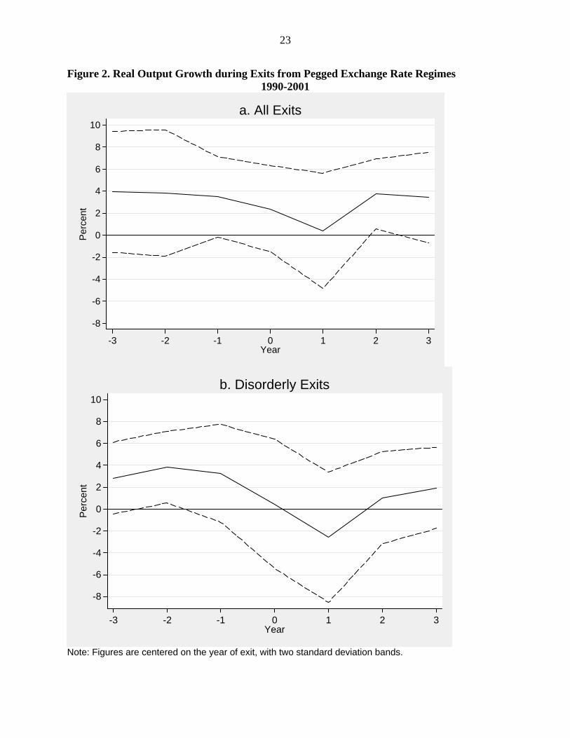
growth is actually negative in the year after exits. Figure 2 presents event windows for the more

recent period of 1990-2001. Comparison with Figure 1 indicates that the severity of output

declines is higher in the more recent period, supporting the view that greater capital mobility has

increased the magnitude of welfare losses associated with financial crises.

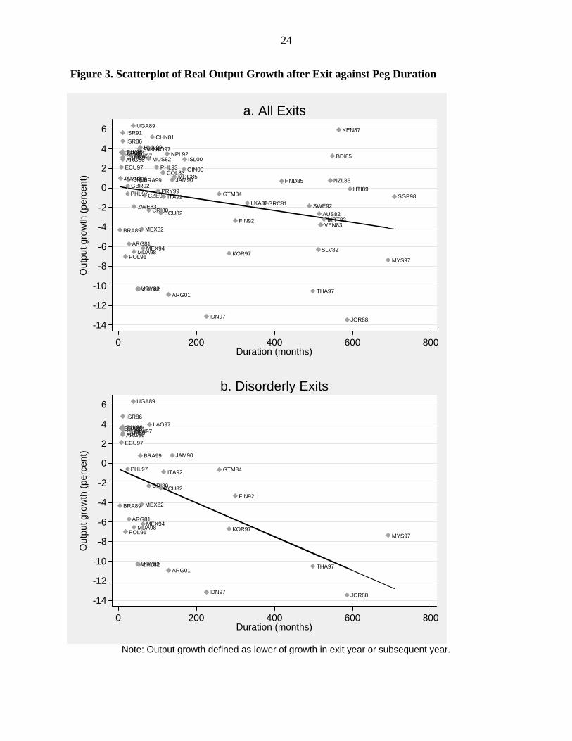
Figure 3 presents scatter plots for GDP growth in either the year of an exit or the year

after (whichever is lower) against the duration (in months) of the regime in place prior to the

exit. For the full sample, a slight negative slope is apparent: the longer the duration of a pegged

2 More specifically, using the Reinhart-Rogoff “natural” classification scheme, they define an exit as occurring when a country moves from categories 1–2, corresponding to pegs or heavily managed exchange rate regimes, to coarse categories 3–6, corresponding to more flexible regimes. A disorderly exit is characterized as one in which the transition is to the “freely falling” category, within 12 months of the original exit. Reinhart and Rogoff (2004) define the exchange rate as freely falling if its rate of depreciation is large, there is high inflation, or a speculative attack against the currency takes place. Note that the sample of Detragiache et al (2005) includes both developing and industrial countries. 3 We omit Iraq’s 1982 exit because of the extreme decline in output, almost 40 percent. Note Detragiache et al treat this episode as an orderly exit.

5

exchange rate regime, the lower (greater) is output growth (decline). When focus is drawn to the

disorderly cases (bottom panel), the negative slope is more pronounced and is significant.

These results are confirmed with simple linear regressions reported in Table 1; the

negative association of output growth following exits with the duration of pegged exchange rate

spells is significant at 5% for the full sample and at better than 1% for the disorderly sample. The

table also reports the results of restricting the sample to 1990 or later. Observe that for the

sample of both orderly and disorderly exit episodes the negative effect of duration is almost

double in magnitude when the 1980s observations are excluded. In contrast, the results for the

disorderly exit episodes alone are roughly the same across periods. This implies that orderly

exits from longer duration pegs have been associated with more severe output declines in the

1990s than in the 1980s.4 One possible reason for this is the greater role of international capital

flows.

These results support the findings of Eichengreen and Masson (1998) and Eichengreen

(1999) that exits from pegged exchange rate regimes have been accompanied by output declines.

In addition, they show that exits from long-lasting pegs, both orderly and disorderly, appear to be

accompanied by particularly large falls in economic activity. We proceed to formulate a model

that explains these stylized facts.

3. Model

The basic framework follows Flood and Marion (1999), a simplified version of Obstfeld

(1996)’s model of a small open economy. Output is determined by inflation surprises and real

shocks:

uy e −−= ππ

where , eπ π are actual and expected inflation, respectively -- equivalent to the rate of domestic

currency devaluation for a small open economy in which purchasing power parity holds, and u is

an adverse productivity shock, ),0(~ 2ufu σ .5 The social loss function attaches a penalty to

inflation (or deflation), deviations of output from a target, and any realignment of the exchange

rate:

4 Unreported regressions confirm this. 5 The natural rate of output is implicitly set to zero.

6

(1) 2 2( )pL y k cβ π χ= + − +

where k (>0) is the target level of output associated with distortions in the economy, pβ is the

relative weight placed by the public on inflation/output losses, i.e. its degree of desired firmness

against inflation, χ is the indicator function,

1 if 00 if 0

πχ

π≠⎧

= ⎨ =⎩,

and c is the fixed cost associated with any exchange rate realignment.

Policy control is delegated to a monetary authority with the following loss function

(1’) 2 2( )M y k cβπ χ= + − + ,

where the authority’s inflation/output loss weight or firmness β differs in general from that of

society pβ . We assume that β is publically known. We deal with the case in which the

equilibrium is time invariant and omit time subscipts.

3.1 Optimal Monetary and Exchange Rate Policy

The monetary authority optimizes by setting the inflation rate -- and the corresponding

devaluation or revaluation rate -- that minimizes the expectation of the loss function (1’). As in

similar models, the productivity shock and public’s expected inflation rate are known by the

monetary authority before choosing the level of inflation, while productivity and the inflation

rate are not ex ante known by the public. This leads to a trigger rule, conditional on the

authority’s anti-inflation firmness β :

(2) if or

10 if

ek u u u u u

u u u

ππ β

⎧ + +> >⎪= +⎨

⎪ > >⎩

where

(1 )

(1 )

e

e

u c k

u c k

β π

β π

≡ + − −

≡ − + − −.

The monetary authority’s ex post loss from fixing or changing the exchange rate, respectively, is

7

(3)

2

2 22

( )

( ) ( )1 1 1

fix e

e edev e e

M k u

k u k uM k u c k u c

β

β

π

π π ββ π πβ β β

= + +

⎛ ⎞ ⎛ ⎞+ + + += + − + + + = + + +⎜ ⎟ ⎜ ⎟+ + +⎝ ⎠ ⎝ ⎠

where the latter is conditional on the regime’s firmness β . Thus, the authority changes the

exchange rate only when u is high enough, i.e. u u> (in which case the currency is devalued) or

low enough, i.e. u uβ< (in which case the currency is revalued), to make dev fixM Mβ β< .6 For

shock realizations u u u> > , the fixed exchange rate is maintained.

The expected social loss function corresponding to the optimal inflation rate, given public

inflation expectations eπ , and public’s anti-inflation weight pβ , is

(4)

22 2

2

22

2

( ) ( ) ( ) ( ) ( )(1 )

( ) ( )(1 )

upe e

u u

upe

E L k u f u du k u c f u du

k u c f u du

β βπ π

β

β βπ

β

∞

−∞

⎧ ⎫+⎪ ⎪= + + + + + +⎨ ⎬+⎪ ⎪⎩ ⎭

⎧ ⎫+⎪ ⎪+ + + +⎨ ⎬+⎪ ⎪⎩ ⎭

∫ ∫

∫

As is well known, because expected inflation eπ enters here both in (i) determining the inflation

rate the authority chooses conditional on preferring to realign and in (ii) determining the

probability of realignment (through ,u u ), the possibility of multiple equilibria arises. Rational

expectation equilibrium implies that public sector’s expected inflation eπ equals the expectation

of inflation ( )E π , where

(5) ( ) ( ) ( )1 1

u e e

u

k u k uE f u du f u duπ ππβ β

∞

−∞

+ + + += +

+ +∫ ∫ .

To gain further insight, let us consider the case where u follows the double exponential

distribution, with zero mean and variance 22 /θ :

(6) ]exp[2

)( uuf θθ−= .

A convenient feature of this distribution is that we can solve for the closed form of (5):7

6 The assumption that the costs of realignment c are the same for devaluations or revaluations implies that adjustment is symmetric. 7 Obstfeld (1996) assumes u is uniformly distributed; Flood and Marion (1999) show how the results are affected by using a normal distribution, with fatter tails than the uniform, implying extreme shocks are more likely to occur. Our assumption of a double exponential permits a tractable analytical solution for a (relatively) fat-tailed distribution.

8

(7)

[ ] [ ]( ){ }( ) [ ] ( ) [ ]

[ ] [ ]( ){ }( ) [ ] ( ) [ ]

[ ] [ ]( ){ }( ) [ ] ( ) [ ]

( ) 1 0.5 exp exp1 if 01 exp 1 exp 1

2

( ) 0.5 exp exp1( ) if 01 exp 1 exp 1

2

( ) 1 0.5 exp exp1 if 01 exp 1 exp 1

2

e

e

e

k u uu uu u u u

k u uE u uu u u u

k u u

u u u u

π θ θ

θ θ θ θ βθ

π θ θπ θ θ θ θ β

θ

π θ θ

θ θ θ θ βθ

⎡ ⎤+ − −⎢ ⎥

< <⎢ ⎥− − − +−⎢ ⎥⎣ ⎦

⎡ ⎤+ − +⎢ ⎥

= < <⎢ ⎥+ − + − ++⎢ ⎥⎣ ⎦

⎡ ⎤+ + − − −⎢ ⎥⎢ ⎥+ − − + − ++⎢ ⎥⎣ ⎦

u u

⎧⎪⎪⎪⎪⎪⎪⎪⎪⎨⎪⎪⎪⎪⎪⎪

< <⎪⎪⎩

The full equilibrium in which ( ) eE π π= is summarized by Figure 4, which graphs expression

(7) as an S-shaped curve for different values of β , together with a o45 line, assuming the

parameter values 8,1.0,06.0 === θkc . The firmness of the policymaker β plays a key role

in determining the equilibrium. For “tough” regimes (i.e. high β ), there is a unique equilibrium,

associated with low expected inflation (e.g. about 5 percent, as at point A for β =0.3). For “soft”

regimes (i.e. low β ), we have a unique equilibrium associated with high inflation (e.g. about 100

percent, as at point B for β =0.1). For intermediate regimes, we have multiple equilibria, with 2

or 3 possible inflation rates (Figure 4 depicts the case where for β = 0.2 there are 3 possible

equilibrium inflation rates -- C1, C2 , C3).

In the Appendix we show that for β close to pβ the multiple equilibria in Figure 4 can

be Pareto ranked by the level of expected inflation by proving the following claim:

Claim 1: Expected social loss ( )E L rises with expected inflation eπ

Assuming that the multiple equilibria occur with equal probability, it follows that the association

between the firmness of the regime and expected inflation is discontinuous in the intermediate

9

range of firmness, and that the move from the multiple equilibrium range to a unique equilibrium

of low inflation is associated with a large drop in expected inflation.

For example, for the parameters used in Figure 4, the minimal level of firmness

associated with a unique low inflation equilibrium is about β = 0.25. (The corresponding S-

shaped curve – not shown -- would just “kiss” the 45o line from below between points C1 and

C2.) For a firmness level somewhat above 0.25, the expected inflation is about 5.5%, whereas for

a firmness level marginally below that level, multiple equilibria emerge and the expected

inflation jumps above 30%. Lower firmness shifts the curve upward, increasing expected

inflation. As noted above, for a low enough firmness level, a unique high inflation equilibrium

arises. For β = 0.1, for example, the unique high inflation equilibrium (at point B) is associated

with expected inflation of roughly 100%.

This discontinuity implies that there are large potential gains from eliminating the

multiple equilibria and is the key for the analysis in the paper. It implies that it is desirable to

bias the choice of the monetary authority’s firmness towards the conservative end of the

available pool, not only in order to mitigate the inflation bias arising from time inconsistency,

but also to eliminate the excessive expected inflation due to multiple equilibria. Achieving these

gains requires picking a monetary authority with a sufficiently high firmness level and hence

conservative bias. Such a bias, however, comes also with costs in the form of a lesser

responsiveness by the authority to shocks. Hence, there is a trade off between the ex-ante gains

from stabilizing expectations and the ex-post costs associated with having a conservative

decision maker who is unwilling to allow the exchange rate to adjust in response to very large

shocks.

3.2 Costly Regime Change

We complete the model by assuming that ex-post the public has the costly option of

replacing the existing monetary regime with one representing the public’s preferences, i.e. a

monetary authority characterized by pβ β= . We denote the cost of regime change by rcc and

assume8

8 It will be shown that this condition implies a non-empty range of discretionary devaluations by the conservative policymaker.

10

(8) 2( )

(1 )(1 )prc

p

cc

β ββ β

−>

+ +,

implying the relative cost of regime change exceeds the relative firmness bias of the existing

monetary authority. It follows that the inflation rate observed with a monetary authority of type β

is

(9)

if or > >1

0 if

if or1

e

rcrc

e

rcrcp

k u u u u u u u

u u uk u u u u u

πβ

π

πβ

⎧ + +> >⎪

+⎪⎪= > >⎨⎪ + +⎪ > >

+⎪⎩

.

where

1 1(1 ) ; (1 )

(1 ) ; (1 )

e erc rc p rc prc

p p

e e

u c k u c k

u c k u c k

β ββ π β πβ β β β

β π β π

⎛ ⎞ ⎛ ⎞+ +≡ + − − ≡ − + − −⎜ ⎟ ⎜ ⎟⎜ ⎟ ⎜ ⎟− −⎝ ⎠ ⎝ ⎠

≡ + − − ≡ − + − −

A monetary authority of type β leaves the exchange rate unchanged for shocks in the range

u u u> > . The regime remains in place when u is higher, but not “too” high, i.e. rcu u u> > (in

which case the currency is devalued) or low enough, but not “too” low, i.e. rcu u u> > (in which

case the currency is revalued). In these ranges the authority will devalue (or revalue) by an

amount 1

ek uππβ

+ +=

+. For very large shocks, however, i.e. orrc rcu u u u> > , it is socially

optimal to replace the regime as well as realign the exchange rate by setting 1

e

rcp

k uππβ

+ +=

+,

which is larger than π since pβ β> .9

9 The expected depreciation rate that prevails in the event of regime change is the same as under a completely flexible exchange rate.

11

To understand this behavior, we compare the ex post social loss function (2) for the cases

of no devaluation ( fixL ), devaluation by a policymaker of firmness type β ( devLβ ), and a regime

change and devaluation set by a (new) policymaker of firmness type pβ (p

rcLβ ):

(10)

2

2 2

22

2

2 2

2

( )

( )1 1

( )(1 )

( )1 1

( )1

p

fix e

e edev e

p

p e

e erc e

p rcp p

p erc

p

L k u

k u k uL k u c

k u c

k u k uL k u c c

k u c c

β

β

π

π πβ πβ β

β βπ

β

π πβ πβ β

βπ

β

= + +

⎛ ⎞ ⎛ ⎞+ + + += + − + + +⎜ ⎟ ⎜ ⎟+ +⎝ ⎠ ⎝ ⎠

+= + + +

+

⎛ ⎞ ⎛ ⎞+ + + += + − + + + +⎜ ⎟ ⎜ ⎟⎜ ⎟ ⎜ ⎟+ +⎝ ⎠ ⎝ ⎠

= + + + ++

Applying (3), the existing monetary authority will not devalue for u shocks in the range

u u u> > , since dev fixM Mβ > . We can also show for shocks in this range that the public will not

prefer a regime change because the welfare loss of doing so is less than that of maintaining the

regime and leaving the exchange rate unchanged, i.e. p

rc fixL Lβ > .

To demonstrate this, note from (10) that p

rc fixL Lβ > implies

( )22( )1

p e erc

p

k u c c k uβ

π πβ

+ + + + > + ++

,

or equivalently,

(11) 21 ( )1

erc

p

c c k uπβ

+ > + ++

.

However, the definitions of ,u u imply

2(1 ) ( ) (1 )ec k u cβ π β− + < + + < + ,

which combined with (8) implies (11) holds. Thus for u u u> > , the existing monetary

authority remains in place and no devaluation occurs.

12

Suppose now that u is large enough (in absolute value) to induce the policymaker to

adjust the exchange rate, but not large enough to prompt a change in regime, e.g. rcu u u> > .

The resultant rate of devaluation is

(12) 1

ek uππβ

+ +=

+,

implying a social welfare loss of dev fixL Lβ < . In this case the public would continue to support

the existing regime as long as the magnitude of devaluation chosen by the policymaker, given by

(12), is not viewed as “too timid” a response to the shock and/or if the cost of regime change is

not too high, i.e. dev rc

pL Lβ β< .

To demonstrate this, note that a regime change would entail a devaluation of magnitude

(12’) 1

e

rcp

k uππβ

+ +=

+

and a welfare loss of rc

pLβ . Thus, the existing regime is maintained if rc dev

pL Lβ β> , or applying (10),

if

(13) 2

22 ( )

(1 ) 1p p e

rcp

k u cβ β β

πβ β

⎛ ⎞+− + + <⎜ ⎟⎜ ⎟+ +⎝ ⎠

,

or equivalently, if

(13’) 1 (1 ) erc rc p

p

u u c kβ β πβ β

+< ≡ + − −

−. 10

10 Note that

2 2

2 2

( )1(1 ) (1 ) (1 )

p p p

p p

β β β β βββ β β

+ −− =

++ + +and condition (8),

( )

2( )1 (1 )

prc

p

cc

β ββ β

−>

+ +, implies

2

(1 )(1 )(1 ) (1 )

( )p

rcp

c cβ β

β ββ β

+ ++ < +

− ; hence rcu u> , i.e., there is a non-empty range of discretionary devaluations

by the conservative policymaker. Note also that the gap between the public’s and the monetary authorities’ welfare

losses in the event of a devaluation not accompanied by a regime change is proportional to the difference between

their respective degree of firmness, since 2

2 22 ( ) ( )

(1 ) 1 1p pdev dev e e

t t t tL M k u k uβ β

β β β ββ π πβ β β

⎛ ⎞+ −− = − + + = + +⎜ ⎟⎜ ⎟+ + +⎝ ⎠

.

13

Thus for rcu u u> > , the shock u is high enough to induce the policymaker to devalue, but not

high enough to prompt a regime change. While the policymaker devalues at a rate that is below

the public’s desired rate ( rcπ π> since pβ β> ), the shock is not high enough to induce a

regime change. This is the down side of the conservative bias: the policymaker is too timid in

the use of discretionary policy. Yet, for this range of shocks, the social cost of regime change

still exceeds the marginal benefit to implementing a higher devaluation rate. Only when rcu u>

is a regime change and a greater magnitude of devaluation desirable. A similar analysis holds

for rcu u u> > and rcu u> .

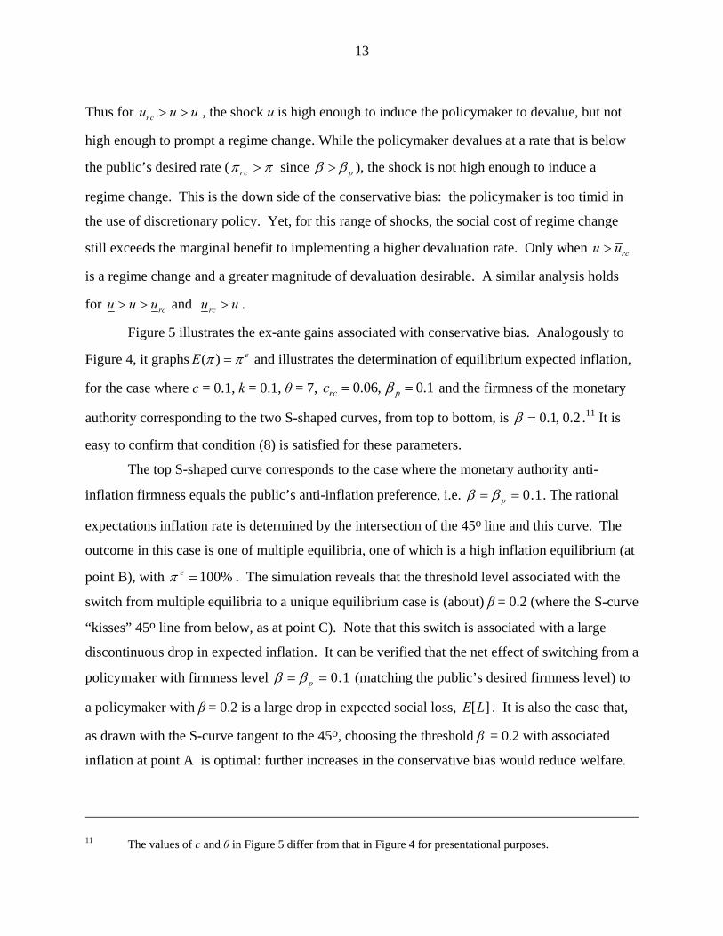
Figure 5 illustrates the ex-ante gains associated with conservative bias. Analogously to

Figure 4, it graphs ( ) eE π π= and illustrates the determination of equilibrium expected inflation,

for the case where c = 0.1, k = 0.1, θ = 7, 0.06, 0.1rc pc β= = and the firmness of the monetary

authority corresponding to the two S-shaped curves, from top to bottom, is 2.0,1.0=β .11 It is

easy to confirm that condition (8) is satisfied for these parameters.

The top S-shaped curve corresponds to the case where the monetary authority anti-

inflation firmness equals the public’s anti-inflation preference, i.e. 0.1pβ β= = . The rational

expectations inflation rate is determined by the intersection of the 45o line and this curve. The

outcome in this case is one of multiple equilibria, one of which is a high inflation equilibrium (at

point B), with %100=eπ . The simulation reveals that the threshold level associated with the

switch from multiple equilibria to a unique equilibrium case is (about) β = 0.2 (where the S-curve

“kisses” 45o line from below, as at point C). Note that this switch is associated with a large

discontinuous drop in expected inflation. It can be verified that the net effect of switching from a

policymaker with firmness level 0.1pβ β= = (matching the public’s desired firmness level) to

a policymaker with β = 0.2 is a large drop in expected social loss, ][LE . It is also the case that,

as drawn with the S-curve tangent to the 45o, choosing the threshold β = 0.2 with associated

inflation at point A is optimal: further increases in the conservative bias would reduce welfare.

11 The values of c and θ in Figure 5 differ from that in Figure 4 for presentational purposes.

14

To understand the determinants of the optimal level of bias, we note that in general, for a

given public anti-inflation preference level pβ , the welfare effect of choosing a more

conservative monetary authority type can be expressed as

(14) [ ] [ ] [ ] e

e

dE L E L E Ld

πβ β π β

∂ ∂ ∂= +

∂ ∂ ∂

The first term of (14) corresponds to the direct welfare effect of greater conservative bias,

holding the expected inflation constant. The second term measures the indirect effect of greater

conservative bias through changing expected inflation. In the Appendix we show that

Claim 2: For a given level of pβ , (i) [ ]/ 0E L β∂ ∂ > , i.e. greater conservative bias increases the

expected social loss, holding expected inflation given; (ii) ( [ ]/ )( / ) 0e eE L π π β∂ ∂ ∂ ∂ < , i.e. greater conservative bias reduces the expected social loss by reducing expected inflation. That the expected loss rises with a more conservative regime follows from the property that in

circumstances leading to exchange rate adjustment, a more conservative decision maker uses

discretion more timidly. A more conservative monetary authority has an opposing effect on

expected loss by reducing expected inflation. Consequently, the welfare effect of the

conservative bias is ambiguous, being the sum of two opposing effects. Choosing the candidate

with the conservative bias sufficiently high enough to eliminate the multiple equilibria would be

optimal if the drop in expected inflation (captured by the second term) dominates the first. This

will be the case if the discrete drop in expected inflation is large enough, as is the situation in

Figure 5. The conservative bias comes, however, with potential ex-post costs: the policy maker

may be “too conservative” when bad shocks hit the economy. In these circumstances, a very bad

state of nature would induce a regime change, and a large discretionary devaluation.

The optimal degree of policy firmness, *β , corresponds to the point of tangency between

the lower S-shaped curve and the 45o ray (e.g. point C in Figure 5), and is associated with the

relatively low expected inflation rate (corresponding to point A ).12 The location of the

12 The discontinuity of expected inflation associated with this equilibrium implies that the optimal bias must

actually exceed*β marginally in order to induce the low inflation equilibrium. More specifically, recall that because

of the knife-edge discontinuity in the effect of β on expected inflation, for β just below the threshold *β there are

multiple equilibria for expected inflation, while for β marginally above *β a unique equilibrium with lower

15

( ) eE π π= curves and this equilibrium are perturbed by variations in the costs of devaluation c

and of regime change, rcc . From (7) it follows that a higher cost of devaluation, reduces the

range where discretionary devaluations take place, thereby shifting the expected inflation curves

downward. A similar result applies for higher costs of regime change, rcc . Consequently, a

higher cost of regime change or higher cost associated with devaluation each reduce the optimal

conservative bias needed to prevent multiple equilibria. That is,

(15) * *

0, 0; 0, 0.e e

rc rc

d d d ddc dc dc dc

π β π β< < < <

We can express this relation in reduced form as: * * * *[ , ] ; / 0, / 0rc rcc c c cβ β β β= ∂ ∂ < ∂ ∂ < .

We next turn to the effects of the exit from an exchange rate regime on output. The

association between the duration of the regime and the magnitude of the output drop following a

devaluation triggered by a regime change is summarized by the following:

Claim 3: Consider a pegged exchange rate regime that is maintained until a large enough

adverse shock induces a regime change and devaluation. The average output decline associated

with the change is larger the longer is the duration of the prior pegged regime.

We prove this claim in several stages. First, we evaluate the factors determining the

output decline associated with a shock large enough to lead to regime change. Next, we

characterize the factors determining the duration of the peg, and identify the factors impacting

both the duration of the peg, and the ultimate cost of the exiting the peg.

Denote by rcu the adverse productivity shock which is large enough to cause a regime

change, i.e. rc rcu u> (see the discussion after (12)). Applying (12’) and the output equation, the

resulting regime change is associated with a negative output gap of

(16) ( ) ( ) ( )1 1

epe e erc

rc rc rc rc rcp p

k uy k k u k u k uβππ π π π

β β+ +

− = − + + = − + + = − + ++ +

expected inflation occurs. This discontinuity also applies to the sign of (14) and the impact of β on expected

welfare: for *β β> ( *β β< ), the impact of greater conservative bias ( [ ] /dE L dβ ) is to reduce (increase) the

public loss.

16

Since rc rcu u> , it follows that

( )1

p erc rc

p

y k k uβ

πβ

− ≤ − + ++

.

Substituting with the definition of rcu from (13’) implies that13

(16’) 1

prc

p

y kβ

φβ

− ≤ −+

where 1 (1 )rc pp

cβφ ββ β

+≡ +

−.

It can be verified readily that 0>rccd

d φ and 0<βφ

dd , implying that a higher cost of regime

change ( rcc ), or a lower conservative bias ( pβ β− ), increase the output gap at the time of the

regime change.14

Further insight is gained by evaluating the duration of a peg.15 Denote the probability of

sustaining the peg in each period by

(17) ( )u

u

f u duΓ = ∫ ,

where, recall from (2), the upper and lower bounds of productivity shocks inducing a devaluation

are given by

(1 ) ; (1 )e eu c k u c kβ π β π≡ + − − ≡ − + − − .

The expected duration of a fixed exchange rate is the probability of sustaining the peg, relative to

the probability of leaving the peg, or16

13 Note that the response of output and inflation to productivity shocks is discontinuous around the magnitude of u that triggers a regime change. That is, for rcu u< ( )/ (1 ) ( )ey k k uβ β π− ≤ − + + + , while for rcu u> the output gap is given by (16).

14 To determine / 0d dφ β < , note that 2

11 / 0.( )

p

p p

ββ ββ β β β

⎧ ⎫ ++⎪ ⎪∂ ∂ = − <⎨ ⎬− −⎪ ⎪⎩ ⎭

15 There are four possible cases for exiting from the current exchange rate peg: (i) devaluation without regime change, (ii) revaluation without regime change, (iii) devaluation with regime change, and (iv) revaluation with regime change. The following discussion focuses only on the first two cases; analysis of the other cases is analogous. 16 This follows from the observation that the expected duration of the peg is:

17

(18) Γ−

Γ1

.

Recall from (15) that a higher cost of regime change has the effect of reducing the

expected inflation eπ and the optimal conservative bias *pβ β− . This implies a higher

probability of sustaining the peg (since the range u u− widens), as well as higher level of

φ (since / 0rcd dcφ > and / 0d dφ β < ).17 Hence, a higher cost of regime change implies, on

average, a longer duration of the peg, and greater output costs associated with the change in

exchange rate, when a large enough adverse shock occurs.

4. Concluding Remarks

In this paper we have presented a simple model in which the conservative bias of an

exchange rate/monetary regime as well the cost of changing an exchange rate regime affects the

tradeoff between anti-inflation credibility gains and the ultimate welfare losses costs incurred

when exiting the peg. In particular, we have shown that greater conservative bias or higher costs

of regime change each reduce expected inflation as long as the regime remains in place.

However, the output costs are correspondingly higher once a sufficiently large adverse shock

prompts an exit from the regime.

This analysis helps understand the explosive ending of many recent pegged exchange rate

regimes, such as that of Argentina in 2001. In our framework the legal anchoring of Argentina’s

currency board regime through the country’s constitution can be interpreted as an effort to raise

the cost of devaluation and regime change. While this effort provided obvious anti-inflation

credibility gains, it also raised the eventual costs of exiting the peg. It apparently prolonged the

duration of the peg, but at a cost of greater loss of output upon the ultimate exit from the peg via

a regime change. The empirical evidence we present suggests that these tradeoffs have relevance

for many countries struggling with the design of exchange rate regimes.

' '1

0 0 1

(1 ) (1 ) (1 ) (1 )1 1

j j j

j j j

j j∞ ∞ ∞

−

= = =

⎡ ⎤ Γ Γ⎡ ⎤Γ − Γ = − Γ Γ Γ = − Γ Γ Γ = − Γ Γ =⎢ ⎥ ⎢ ⎥− Γ − Γ⎣ ⎦⎣ ⎦∑ ∑ ∑ .

17 The impact of higher devaluation cost c on the duration of the peg is the sum of two opposing forces: (i) a positive effect through lower expected inflation and an increase in u , and (ii) a negative effect through a lower optimal conservative bias that reduces u . It can be shown that the first effect dominates, i.e. a higher devaluation cost c increases the peg duration. A similar result applies for a higher regime change cost.

18

References

Agenor, Richard and Peter Montiel, 1999. Development Macroeconomics, 2nd edition, Princeton Press.

Cukierman, Alex and Liviatan, Nissan, 1991. "Optimal accommodation by strong policymakers

under incomplete information," Journal of Monetary Economics, 27(1), pp. 99-127. Detragiache,Enrica, Ashoka Mody, and Eisuke Okada, 2005. “Exits from heavily managed

exchange rate regimes,” IMF WP/05/39. Eichengreen, B. 1999. “Kicking the habit: moving from pegged rates to greater exchange rate

flexibility,” Economic Journal, March, C1-C14. Eichengreen , Barry, and Paul Masson, 1998. “Exit strategies: Policy options for countries

seeking greater exchange rate flexibility,” Occasional Paper No. 98/168 (Washington: International Monetary Fund).

Flood, R. and Marion, N. 1999. “Perspectives on recent currency crisis literature.” International

Journal of Finance and Economics, Vol 4, No. 1, 1-26. Husain, M. Aasim., Ashoka Mody and Kenneth S. Rogoff. 2005. “Exchange rate regime

durability and performance in developing versus advanced economies,” Journal of Monetary Economics, 52 ( 1), pp. 35-64

Klein, Michael W. and Nancy Marion. 1997. “Explaining the duration of exchange-rate

pegs,” Journal of Development Economics, 54(2), 387-404. Lohmann, Susanne. 1992. “The optimal degree of commitment: Credibility and flexibility.”

American Economic Review, 82(1), March, 273-286. Obstfeld, M. 1996. “Models of currency crises with self fulfilling features,” European Economic

Review 40, April, 1037-1048. Obstfeld, M. and K. Rogoff, 1996. Foundations of International Economics, MIT Press.

Rogoff, K. 1985. “The optimal degree of commitment to an intermediate monetary target,”

Quarterly Journal of Economics, 1169-89. Reinhart, Carmen, and Kenneth Rogoff, 2004, “The modern history of exchange rate

arrangements: A reinterpretation,” Quarterly Journal of Economics, Vol. 119, No. 1, pp. 1–48.

19

Appendix

A. Claim 1: Expected social welfare loss increases with expected inflation, for ek π<− :

Proof: Equation (4) and the envelope theorem imply that for β close to pβ

(A1) ( ) 2 ( ) ( )e

E L y u f u dudπ

∞

−∞

∂≅ ∫ ,

where

(A2)

2

2

2

2

( ) for(1 )

( ) for

( ) for(1 )

pe

e

pe

k u u u

y u k u u u u

k u u u

β βπ

βπ

β βπ

β

⎧ ++ + <⎪

+⎪⎪= + + < <⎨⎪ +⎪ + + <⎪ +⎩

.

and ,u u are defined by (2). Inspection of (A2) reveals that )(uy is a piece-wise linear

function; and )(uy is a symmetric function of u around ke −=π . Recall that )(uf is symmetric

around 0=u . Hence,

(A3) for ke −=π , 0)(=

∂

∂eLE

π.

Note also that 0][

)(2

2>

∂

∂e

LEπ

. Consequently, the expected loss function is minimized at ke −=π ,

and for ke −>π , higher expected inflation increases the expected loss function.

B. Claim 2: (i) [ ] / 0E L β∂ ∂ > , (ii) ( [ ] / )( / ) 0e eE L π π β∂ ∂ ∂ ∂ <

Proof: Recall the definitions of , ,p

fix dev rcL L Lβ β in (10) for the social loss in the absence of no

devaluation, devaluation by a policy maker of type β , and regime change followed by

devaluation set by a policymaker of type pβ , respectively. The expected social loss is

(B1) [ ] ( ) ( ) ( ) ( ) ( )rc rc

p p

rcrc

uu u urc dev fix dev rc

u u uu

E L L f u du L f u du L f u du L f u du L f u duβ β β β

∞

−∞

= + + + +∫ ∫ ∫ ∫ ∫

Applying the envelope theorem, it follows that increasing the conservative bias affects the

expected loss function by the sum of two terms, reflecting the direct effect of greater bias and the

indirect effect through inflation expectations, respectively:

20

(B2) [ ] [ ] [ ] e

e

dE L E L E Ld

πβ β π β

∂ ∂ ∂= +

∂ ∂ ∂ .

The first term is given by

(B3)

( )

2 23

2

[ ] 2 ( ) ( ) ( ) ( )(1 )

1 (1 ) ( ) ( ) 02 (1 )

rc

rc

u upe e

u u

p

E L k u f u du k u f u du

c c f u f u

β βπ π

β β

β ββ

β

⎛ ⎞ −∂ ⎜ ⎟= + + + + +⎜ ⎟∂ +⎝ ⎠

−+ + + >

+

∫ ∫.

Hence [ ] 0E Lβ

∂>

∂, implying that increasing the conservative bias reduces the actual exchange

rate adjustment in the range where the policymaker would devalue (or revalue), thereby reducing

social welfare.

In order to sign the second term, the impact of β on welfare through changing

expectations, note that for β close to pβ

2

2

2

2

[ ](B4) 2 ( ) ( ) 2 ( ) ( )(1 )

2 ( ) ( ) 2 ( ) ( )(1 ) 1

2 ( ) ( ) 2 ( ) ( ) 2 ( ) 01 1 1

rc

rcrc

rc

uupe e

eu u

up pe e

puu

up p pe e e

p p p

E L k u f u du k u f u du

k u f u du k u f u du

k u f u du k u f u du k

β βπ π

π β

β β βπ π

β β

β β βπ π π

β β β

∞

∞

−∞ −∞

+∂= + + + + +

∂ +

++ + + + + +

+ +

+ + + > + + = + >+ + +

∫ ∫

∫ ∫

∫ ∫

Hence, higher expected inflation is welfare reducing:

(B5) 0][>

∂

∂eLE

π.

Consequently, since higher β reduces expected inflation (i.e. 0eπ

β∂

<∂

), the lower expected

inflation induced by a greater conservative bias is welfare enhancing:

(B6) [ ] 0e

e

E L ππ β

∂ ∂<

∂ ∂.

The effect of greater bias depends on the sum of the effects reported by (B3) and (B4) [see (B2)].

21

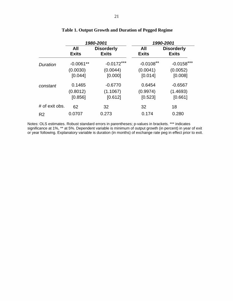
Table 1. Output Growth and Duration of Pegged Regime

1980-2001 1990-2001

All

Exits Disorderly

Exits All

Exits Disorderly

Exits

Duration -0.0061** -0.0172*** -0.0108** -0.0158*** (0.0030) (0.0044) (0.0041) (0.0052) [0.044] [0.000] [0.014] [0.008]

constant 0.1465 -0.6770 0.6454 -0.6567 (0.8012) (1.1067) (0.9974) (1.4693) [0.856] [0.612] [0.523] [0.661]

# of exit obs. 62 32 32 18

R2 0.0707 0.273 0.174 0.280

Notes: OLS estimates. Robust standard errors in parentheses; p-values in brackets. *** indicates significance at 1%, ** at 5%. Dependent variable is minimum of output growth (in percent) in year of exit or year following. Explanatory variable is duration (in months) of exchange rate peg in effect prior to exit.

22

Figure 1. Real Output Growth during Exits from Pegged Exchange Rate Regimes 1980-2001

-8

-6

-4

-2

0

2

4

6

8

10

Perc

ent

-3 -2 -1 0 1 2 3Year

a. All Exits

-8

-6

-4

-2

0

2

4

6

8

10

Perc

ent

-3 -2 -1 0 1 2 3Year

b. Disorderly Exits

Note: Figures are centered on the year of exit, with two standard deviation bands.

23

Figure 2. Real Output Growth during Exits from Pegged Exchange Rate Regimes 1990-2001

-8

-6

-4

-2

0

2

4

6

8

10

Per

cent

-3 -2 -1 0 1 2 3Year

a. All Exits

-8

-6

-4

-2

0

2

4

6

8

10

Per

cent

-3 -2 -1 0 1 2 3Year

b. Disorderly Exits

Note: Figures are centered on the year of exit, with two standard deviation bands.

24

Figure 3. Scatterplot of Real Output Growth after Exit against Peg Duration

ARG81

ARG86

ARG01

AUS82

BRA86

BRA89

BRA99

BDI85

CHL82

CHN81

COL83

CRI80

CZE96

ECU82

ECU97

SLV82

FIN92

GRC81

GTM84

GTM89

GIN00

HTI89HND85

HUN99

ISL00

IDN97

ISR86

ISR89

ISR91

ITA92

JAM90JAM93

JOR88

KEN87

KOR97

LAO97

MDG85

MWI97

MYS97

MRT83

MUS82

MEX82

MEX94MDA98

NPL92

NZL85

PRY99

PHL93

PHL97

POL91

SGP98

SVK97

LKA00 SWE92

TJK98

THA97

GBR92

UGA89

URY82

URY91

VEN83

ZWE83

-14

-12

-10

-8

-6

-4

-2

0

2

4

6

Out

put g

row

th (p

erce

nt)

0 200 400 600 800Duration (months)

a. All Exits

ARG81

ARG86

ARG01

BRA86

BRA89

BRA99

CHL82

CRI80ECU82

ECU97

FIN92

GTM84

GTM89

IDN97

ISR86

ITA92

JAM90

JOR88

KOR97

LAO97MWI97

MYS97

MEX82

MEX94MDA98

PHL97

POL91

TJK98

THA97

UGA89

URY82

URY91

-14

-12

-10

-8

-6

-4

-2

0

2

4

6

Out

put g

row

th (p

erce

nt)

0 200 400 600 800Duration (months)

b. Disorderly Exits

Note: Output growth defined as lower of growth in exit year or subsequent year.

25

Figure 4. Expected Inflation and Multiple Equilibria, with Costly Devaluation

( )E π

eπ Note: Plotted curves correspond (from top to bottom) to anti-inflation firmness levels of

0.1, 0.2, 0.3β = , respectively, for 0.06, 0.1, 8c k θ= = = . The straight solid line from the origin is the 45 degree ray.

. A

B. β = 0.1 β = 0.2 β = 0.3

C1 .

C2 . C3 .

26

Figure 5. Expected Inflation and Multiple Equilibria, with Costly Regime Change

( )E π

eπ

Notes: Plotted curves assume 0.1, 0 .06, 0.1, 0.1, 7p rcc c kβ θ= = = = = . The top bolded curve determines expected inflation for a monetary authority with firmness pβ β= = 0.1. The bottom curve determines expected inflation for an authority with firmness 0.2β = that exceeds the public’s preference. The solid straight line from the origin is the 45 degree ray.

β = 0.2

β = 0.1 C

B .

.A