Lecture notes for the course

554017 Advanced Computational Chemistry

Pekka Manninen

2009

2

Contents

1 Many-electron wave functions 7

1.1 Molecular Schrodinger equation . . . . . . . . . . . . . . . . . . . . . . . . 71.1.1 Helium-like atom . . . . . . . . . . . . . . . . . . . . . . . . . . . . 9

1.2 Molecular orbitals: the first contact . . . . . . . . . . . . . . . . . . . . . . 101.2.1 Dihydrogen ion . . . . . . . . . . . . . . . . . . . . . . . . . . . . . 10

1.3 Spin functions . . . . . . . . . . . . . . . . . . . . . . . . . . . . . . . . . . 121.4 Antisymmetry and the Slater determinant . . . . . . . . . . . . . . . . . . 13

1.4.1 Approximate wave functions for He as Slater determinants . . . . . 141.4.2 Remarks on “interpretation” . . . . . . . . . . . . . . . . . . . . . . 151.4.3 Slater method . . . . . . . . . . . . . . . . . . . . . . . . . . . . . . 151.4.4 Helium-like atom revisited . . . . . . . . . . . . . . . . . . . . . . . 161.4.5 Slater’s rules . . . . . . . . . . . . . . . . . . . . . . . . . . . . . . 17

1.5 Further reading . . . . . . . . . . . . . . . . . . . . . . . . . . . . . . . . . 181.6 Exercises for Chapter 1 . . . . . . . . . . . . . . . . . . . . . . . . . . . . . 18

2 Exact and approximate wave functions 19

2.1 Characteristics of the exact wave function . . . . . . . . . . . . . . . . . . 192.2 The Coulomb cusp . . . . . . . . . . . . . . . . . . . . . . . . . . . . . . . 21

2.2.1 Hamiltonian for a He-like atom . . . . . . . . . . . . . . . . . . . . 212.2.2 Coulomb and nuclear cusp conditions . . . . . . . . . . . . . . . . . 212.2.3 Electron correlation . . . . . . . . . . . . . . . . . . . . . . . . . . . 22

2.3 Variation principle . . . . . . . . . . . . . . . . . . . . . . . . . . . . . . . 232.3.1 Linear ansatz . . . . . . . . . . . . . . . . . . . . . . . . . . . . . . 232.3.2 Hellmann–Feynman theorem . . . . . . . . . . . . . . . . . . . . . . 242.3.3 The molecular electronic virial theorem . . . . . . . . . . . . . . . . 25

2.4 One- and N -electron expansions . . . . . . . . . . . . . . . . . . . . . . . . 262.5 Further reading . . . . . . . . . . . . . . . . . . . . . . . . . . . . . . . . . 282.6 Exercises for Chapter 2 . . . . . . . . . . . . . . . . . . . . . . . . . . . . . 28

3 Molecular integral evaluation 31

3.1 Atomic basis functions . . . . . . . . . . . . . . . . . . . . . . . . . . . . . 313.1.1 The Laguerre functions . . . . . . . . . . . . . . . . . . . . . . . . . 323.1.2 Slater-type orbitals . . . . . . . . . . . . . . . . . . . . . . . . . . . 33

3

3.1.3 Gaussian-type orbitals . . . . . . . . . . . . . . . . . . . . . . . . . 343.2 Gaussian basis sets . . . . . . . . . . . . . . . . . . . . . . . . . . . . . . . 353.3 Integrals over Gaussian basis sets . . . . . . . . . . . . . . . . . . . . . . . 37

3.3.1 Gaussian overlap distributions . . . . . . . . . . . . . . . . . . . . . 383.3.2 Simple one-electron integrals . . . . . . . . . . . . . . . . . . . . . . 383.3.3 The Boys function . . . . . . . . . . . . . . . . . . . . . . . . . . . 393.3.4 Obara–Saika scheme for one-electron Coulomb integrals . . . . . . . 403.3.5 Obara–Saika scheme for two-electron Coulomb integrals . . . . . . . 41

3.4 Further reading . . . . . . . . . . . . . . . . . . . . . . . . . . . . . . . . . 433.5 Exercises for Chapter 3 . . . . . . . . . . . . . . . . . . . . . . . . . . . . . 43

4 Second quantization 45

4.1 Fock space . . . . . . . . . . . . . . . . . . . . . . . . . . . . . . . . . . . . 454.1.1 Creation and annihilation operators . . . . . . . . . . . . . . . . . . 464.1.2 Number-conserving operators . . . . . . . . . . . . . . . . . . . . . 48

4.2 The representation of one- and two-electron operators . . . . . . . . . . . . 494.3 Commutators and anticommutators . . . . . . . . . . . . . . . . . . . . . . 51

4.3.1 Evaluation of commutators and anti-commutators . . . . . . . . . . 524.4 Orbital rotations . . . . . . . . . . . . . . . . . . . . . . . . . . . . . . . . 534.5 Spin in second quantization . . . . . . . . . . . . . . . . . . . . . . . . . . 53

4.5.1 Operators in the orbital basis . . . . . . . . . . . . . . . . . . . . . 544.5.2 Spin properties of determinants . . . . . . . . . . . . . . . . . . . . 57

4.6 Further reading . . . . . . . . . . . . . . . . . . . . . . . . . . . . . . . . . 584.7 Exercises for Chapter 4 . . . . . . . . . . . . . . . . . . . . . . . . . . . . . 58

5 Hartree–Fock theory 61

5.1 The Hartree–Fock approximation . . . . . . . . . . . . . . . . . . . . . . . 615.2 Restricted and unrestricted Hartree–Fock theory . . . . . . . . . . . . . . . 63

5.2.1 Hartree–Fock treatment of H2 . . . . . . . . . . . . . . . . . . . . . 635.3 Roothaan–Hall equations . . . . . . . . . . . . . . . . . . . . . . . . . . . . 64

5.3.1 On the convergence of the SCF method . . . . . . . . . . . . . . . . 665.3.2 Integral-direct SCF . . . . . . . . . . . . . . . . . . . . . . . . . . . 68

5.4 Further reading . . . . . . . . . . . . . . . . . . . . . . . . . . . . . . . . . 695.5 Exercises for Chapter 5 . . . . . . . . . . . . . . . . . . . . . . . . . . . . . 69

6 Configuration interaction 73

6.1 Configuration-interaction wave function . . . . . . . . . . . . . . . . . . . . 736.1.1 Single-reference CI wave functions . . . . . . . . . . . . . . . . . . . 746.1.2 Multi-reference CI wave functions . . . . . . . . . . . . . . . . . . . 746.1.3 Optimization of the CI wave function . . . . . . . . . . . . . . . . . 756.1.4 On the disadvantages of the CI approach . . . . . . . . . . . . . . . 75

6.2 Multi-configurational SCF theory . . . . . . . . . . . . . . . . . . . . . . . 766.2.1 MCSCF wave function of H2 . . . . . . . . . . . . . . . . . . . . . . 76

4

6.2.2 Selection of the active space . . . . . . . . . . . . . . . . . . . . . . 776.3 Further reading . . . . . . . . . . . . . . . . . . . . . . . . . . . . . . . . . 796.4 Exercises for Chapter 6 . . . . . . . . . . . . . . . . . . . . . . . . . . . . . 79

7 Description of dynamical correlation 81

7.1 Coupled-cluster theory . . . . . . . . . . . . . . . . . . . . . . . . . . . . . 817.1.1 The CC Schrodinger equation . . . . . . . . . . . . . . . . . . . . . 817.1.2 The coupled-cluster exponential ansatz . . . . . . . . . . . . . . . . 827.1.3 CI and CC models compared . . . . . . . . . . . . . . . . . . . . . 837.1.4 On coupled-cluster optimization techniques . . . . . . . . . . . . . . 867.1.5 The closed-shell CCSD model . . . . . . . . . . . . . . . . . . . . . 877.1.6 The equation-of-motion coupled-cluster method . . . . . . . . . . . 887.1.7 Orbital-optimized coupled-cluster theory . . . . . . . . . . . . . . . 88

7.2 Perturbation theory . . . . . . . . . . . . . . . . . . . . . . . . . . . . . . . 897.3 Local correlation methods . . . . . . . . . . . . . . . . . . . . . . . . . . . 917.4 Further reading . . . . . . . . . . . . . . . . . . . . . . . . . . . . . . . . . 937.5 Exercises for Chapter 7 . . . . . . . . . . . . . . . . . . . . . . . . . . . . . 93

8 Performance of the electronic-structure models 97

8.1 Molecular equilibrium geometries . . . . . . . . . . . . . . . . . . . . . . . 978.2 Molecular dipole moments . . . . . . . . . . . . . . . . . . . . . . . . . . . 998.3 Reaction enthalpies . . . . . . . . . . . . . . . . . . . . . . . . . . . . . . . 1028.4 Notes on total electronic energies . . . . . . . . . . . . . . . . . . . . . . . 102

5

6

Chapter 1

Many-electron wave functions

1.1 Molecular Schrodinger equation

The Schrodinger equation for a system of N electrons is1

HΨ(x1,x2, . . . ,xN) = EΨ(x1,x2, . . . ,xN), (1.1)

where H is the molecular Hamiltonian, which is for a molecule that contains N electronsand K nuclei (assumed to be fixed in space)

H =

N∑

i=1

hi +

N∑

i=1

N∑

j=i+1

gij, (1.2)

where hi is the one-electron Hamiltonian of electron i moving in an electrostatic potentialcaused by the nuclei, and gij is the interaction between the electrons i and j:

hi = −1

2∇2

i −K∑

I=1

ZI

|ri −RI |; gij =

1

|ri − rj |. (1.3)

The eigenfunctions or wave functions Ψ(x1, . . . ,xN) describe the electronic structure andproperties of the molecule. x are used to collectively symbolize all variables needed torefer to particles; here the position and the internal degree of freedom, spin. It is necessarythat the wave function is square-integrable,

∫

Ψ⋆(x1,x2, . . . ,xN)Ψ(x1,x2, . . . ,xN)dx1dx2 · · · dxN = K (K finite). (1.4)

Usually we assume that the wave function is normalized, i.e., K = 1.The corresponding eigenvalues are in the present context the quantized energy levels of

the electronic “cloud” of the molecule. Any two eigenfunctions that correspond to different

1In atomic units used throughout this course, where ~ = me = 4πǫ0 ≡ 1; c = 1/α ≈ 137.

7

energy values Em, En possess the orthogonality property

∫

Ψ⋆mΨndx1dx2 · · · dxN = 0. (1.5)

Even if two or more eigenvalues happen to be identical, corresponding to a degeneratestate of the system, the different eigenfunctions may still be assumed orthogonal.

If we would like to include the effects of nuclear motion, the molecular Hamiltonianbecomes (now restricting to electrostatic forces only)

H = He + Hn + Hen (1.6)

He = −1

2

∑

i

∇2i +

1

2

∑

ij

′gij

Hn = −1

2

∑

I

1

mI∇2

I +1

2

∑

IJ

′ZIZJ gIJ

Hen = −∑

I

∑

i

ZI

rIi

.

The wave function is correspondingly dependent on both the electron and nuclear variables.Usually, because of the large ratio mn/me, it is a good approximation to separate these,and we may turn our attention to the electronic problem. This is referred to as the Born–Oppenheimer approximation. The nuclear-motion Schrodinger equation plays, however, acentral role in molecular spectroscopy. The motion of nuclei can sometimes affect eventhose properties that are considered electronic. This is the case e.g. in the Jahn–Tellereffect and the Renner effect. For fixed nuclei, we can write the total energy of the systemsimply as

Etot = Eelectronic +1

2

∑

IJ

′ ZIZJ

|RI − RJ |. (1.7)

Eq. (1.1) provides a basis for molecular quantum mechanics and all the static electronicproperties of the molecule may be obtained by expectation values of the appropriate Her-mitian operators or using perturbation theory. However, we should note the limitations ofthis model:

• Limitations in the Hamiltonian: non-relativistic kinematics, instant interactions, andthe Born–Oppenheimer approximation (that implies T = 0)

• Eq. (1.1) is soluble exactly only for a few trivial one-electron systems, such ashydrogen-like atom or the molecule H+

2 (see Exercise 1.1)

• Real experiments are not carried out for an isolated molecule, and observation alwaysinvolves interaction with the system, and thus a time-independent description is notsufficient; but the time-independent form of (1.1), HΨ = i∂Ψ/∂t, should be applied.

8

1.1.1 Helium-like atom

For a helium-like atom with a point-like nucleus of charge Z the electronic Hamiltonian,Eq. (1.2), is

H = h1 + h2 + g12 = −1

2∇2

1 −Z

r1− 1

2∇2

2 −Z

r2+

1

r12.

Due to g12, this is a three-body problem, and thereby no closed form solution exists forthe eigenvalue equation (1.1). We start our consideration by an approximation, where g12

is set to zero, i.e. H0 = h1 + h2. We can separate the variables in the eigenvalue equationH0Ψ0 = EΨ0 by substituting2

Ψ0 = Φ(r1, r2) = χ1(r1)χ2(r2),

to the eigenvalue equation and dividing by Φ, obtaining

h1χ1(r1)

χ1(r1)+h2χ2(r2)

χ2(r2)= E,

meaning that Φ is a solution if (denoting E = ǫ1 + ǫ2)

h1χ1(r1) = ǫ1χ1(r1)

h2χ2(r2) = ǫ2χ2(r2),

meaning that χ1 and χ2 are solutions of the one-electron eigenvalue problem hχ = ǫχ. Φis a simultaneous eigenstate of the operators h1 and h2,

h1Φ(r1, r2) = ǫ1Φ(r1, r2)

h2Φ(r1, r2) = ǫ2Φ(r1, r2).

The 1-electron 1-center eigenfunctions that are solutions to the one-electron eigenvalueproblem (this holds only in the absence of g) are the same with the solutions of theSchrodinger equation for a hydrogen-like atom (note the factor Z),

χnlm(r, θ, ρ) = Rnl(r)Ylm(θ, ρ), (1.8)

consisting of the radial part

Rnl(r) =

(2Z

n

)3/2√

(n− l − 1)!

2n(n+ 1)!

(2Zr

n

)l

L2l+1n−l−1

(2Zr

n

)

exp

(

−Zrn

)

(1.9)

and a spherical harmonic function, explicitly expressed as

Ylm(θ, ρ) =

√

2l + 1

4π

(l −m)!

(l +m)!Pm

l (cos θ) exp(imρ). (1.10)

2Considering only the variables r (position vectors), which in this case are most conveniently represented as the variables of spherical

coordinates, r = (r, θ, ρ)

9

In the above, L denotes the associated Laguerre polynomials

Lαn(x) =

1

n!exp(x)x−α dn

dxn

[exp(−x)xn+α

](1.11)

and P the Legendre polynomials

Pml (x) =

(−1)m

2ll!(1 − x2)m/2 d

l+m

dxl+m(x2 − 1)l; P−m

l = (−1)m (l −m)!

(l +m)!Pm

l (x). (1.12)

These shall be referred to as atomic orbitals (AO). However, this is used also for otheratomic-centered functions with different radial parts, such as sc. Slater- or Gaussian-typefunctions.

1.2 Molecular orbitals: the first contact

When moving from atoms to molecules, the first complication is that even the one-electroneigenfunctions, even when g = 0, are not obtainable in closed form. Instead of the1s, 2s, 2p, . . . AOs we need polycentric molecular orbitals (MO) that describe the states ofa single electron spread around the whole nuclear framework.

1.2.1 Dihydrogen ion

The one-electron eigenvalue equation in the case of hydrogen molecule ion H+2 is hφ = ǫφ,

where

h = −1

2∇2 −

(1

rA+

1

rB

)

.

This may be solved with high accuracy in confocal elliptic coordinates, the solution beinga product of three factors that are in turn solutions of three separate differential equations.We will, however, go immediately to approximations. It is reasonable to expect that

φ(r) ∼ cAχA100(r) (densities close to nucleus A)

φ(r) ∼ cBχB100(r) (densities close to nucleus B)

where cA and cB are some numerical factors. An appropriate trial MO would then be

φ(r) = cAχA100(r) + cBχ

B100(r).

Due to the symmetry of the molecule, it is reasonably to assume that there is no higherdensity in the other end than in the other; therefore

|φ(r)|2 = c2A[χA100(r)]

2 + c2B[χB100(r)]

2 + 2cAcBχA100(r)χ

B100(r),

10

n = 1 n = 2 n = 3l = 0 l = 0 l = 1 l = 0 l = 1 l = 2

m = 0

m = 1

m = 2

Table 1.1: Some lowest-energy solutions χnlm (Z = 1) (blue for positive, orange for negative phase)

11

Figure 1.1: The two lowest MOs of H+2 .

implies that cB = ±cA. Thus, it appears that we can construct two rudimentary MOs fromthe 1s AOs on the two centers, denoted by

φ1(r) = c′A[χA100(r) + χB

100(r)]

φ2(r) = c′B[χA100(r) − χB

100(r)],

where the remaining numerical factors c′A and c′B are to be chosen so that the wave functionswill be normalized. These are sketched in Figure 1.1.

MOs build up this way, in linear combination of atomic orbitals (LCAO), are of greatimportance throughout molecular quantum mechanics.

1.3 Spin functions

It is well-known that a single electron is not completely characterized by its spatial wavefunction φ(r), but an “intrinsic” angular momentum, spin, is required to explain e.g. lineemission spectra of atoms in an external magnetic field. Therefore we must introduce aspin variable ms in addition to r. We further associate operators sx, sy and sz with thethree components of spin angular momentum. We will adopt x as a variable taking intoaccount both degrees of freedom, ms and r, and then introduce spin-orbitals

ψ(x) = φ(r)σ(ms). (1.13)

σ describes the spin state and is a solution of an eigenvalue equation szσ = λσ.If the orbital state is of energy ǫ, then

hψ = ǫψ (1.14)

szψ = λψ, (1.15)

and ψ is a state in which an electron simultaneously has definite energy and z-componentof spin.

12

According to observations, the eigenvalue equation (1.15) has only two solutions forelectrons:

szα =1

2α; szβ = −1

2β

often referred to as “spin-up” and “spin-down”. Therefore an orbital φ yields two possiblespin-orbitals, ψ = φα and ψ′ = φβ with the normalization and orthogonality properties

∫

α⋆αdms =

∫

β⋆βdms = 1,

∫

α⋆βdms =

∫

β⋆αdms = 0. (1.16)

Also the total spin operators

Sz =N∑

i=1

si,z (1.17)

S2 =

N∑

i=1

s2i =

N∑

i=1

(s2

i,x + s2i,y + s2

i,z

)(1.18)

with eigenvalues of M and S(S + 1), respectively, are needed in the discussion of many-electron system. They commute with a spin-free electronic Hamiltonian; and any exactstationary state Ψ is an eigenfunction of them.

1.4 Antisymmetry and the Slater determinant

The fact that electrons are indistinguishable, i.e. |Ψ(x1,x2)|2 = |Ψ(x2,x1)|2, leads to (whengeneralized for N electrons) two possibilities for a wave function:

PΨ(x1,x2, . . . ,xN ) = Ψ(x1,x2, . . . ,xN) symmetric wave function

PΨ(x1,x2, . . . ,xN ) = εP Ψ(x1,x2, . . . ,xN) antisymmetric wave function

where the operator P permutes the arguments and εP is +1 for an even and −1 for an oddnumber of permutations.

The choice for an system consisting of N electrons is once and for all determined by theantisymmetry principle (Pauli exclusion principle): The wave function Ψ(x1,x2, . . . ,xN)that describes any state of an N -electron system is antisymmetric under any permutationof the electrons.

Let us now work out the N -electron wave function. We start by introducing a productfunction of one-electron wave functions (spin-orbitals):

Θ(x1,x2, . . . ,xN) = ψ1(x1)ψ2(x2) · · ·ψN (xN). (1.19)

To yield a fully antisymmetric wave function, A number of differently permuted prod-uct functions must be combined. The combination of permutations is most conveniently

13

expressed as a Slater determinant

Φ(x1,x2, . . . ,xN) = M

∣∣∣∣∣∣∣∣

ψ1(x1) ψ2(x1) · · · ψN (x1)ψ1(x2) ψ2(x2) · · · ψN (x2)

......

. . ....

ψ1(xN) ψ2(xN) · · · ψN (xN)

∣∣∣∣∣∣∣∣

, (1.20)

by which all symmetric permutations are automatically rejected, and thus the Pauli prin-ciple is fulfilled. Expanded in Slater determinants the exact wave function is written as

Ψ(x1,x2, . . . ,xN) =∑

k

ckΦk(x1,x2, . . . ,xN). (1.21)

The normalization factorM is reasoned in the following way: when expanded, Φ consistsof N ! products, and thus an integrand Φ⋆Φ would consist of (N !)2 products, each of a form±[ψ1(xi)ψ2(xj) · · ·ψN (xk)][ψ1(xi′)ψ2(xj′) · · ·ψN(xk′)]. It is evident that unless i = i′, j =j′ etc. in a particular product, the product will give no contribution to the result, due to theorthogonality of spin-orbitals. Therefore, there are N ! non-vanishing contributions, and asevery contribution is equal to 1 with normalized spin-orbitals, we have

∫Φ⋆Φdx1 · · ·dxN =

M2N !, hence the normalization factor has the value M = (N !)−1/2.

1.4.1 Approximate wave functions for He as Slater determinants

The Slater determinant of the configuration (1s)2 of a helium atom in the minimal orbitalbasis is

Φ =1√2

∣∣∣∣

χ100(r1)α(ms1) χ100(r1)β(ms1)χ100(r2)α(ms2) χ100(r2)β(ms2)

∣∣∣∣≡ 1√

2|1sα 1sβ|.

Note the abbreviated notation that will be used quite extensively hereafter: only thediagonal elements are displayed, and the explicit expression of variables is omitted – theleft-right order of the variables in this notation will be 1, 2, 3, .... Also, note that we havedenoted χnlm’s with their corresponding AO labels.

The proper antisymmetric wave functions for the excited 1s2s configuration are in turn

Φ2 =1√2|1sα 2sα|

Φ3 =1

2(|1sα 2sβ| + |1sβ 2sα|)

Ψ4 =1√2|1sβ 2sβ|

Ψ5 =1

2(|1sα 2sβ| − |1sβ 2sα|) .

14

1.4.2 Remarks on “interpretation”

What is the physical meaning of the wave functions introduced earlier? First of all, thegeneral formulation of quantum mechanics is concerned only with symbolic statements in-volving relationships between operators and operands, and is independent of the employed“representation” or “interpretation”.

• In a very “nihilistic” interpretation, MOs as well as spin-orbitals are just mathemat-ical means for the solution of the molecular Schrodinger equation and no meaningcan be given for them or even their squared norms.

• Perhaps more commonly, a spin-orbital ψ(x) itself is thought to be just a mathemat-ical entity but |ψ(x)|2dx is taken to be the probability of a point-like electron beingin an element dx, that is, in volume element dr with spin between ms and ms +dms.|φ(r)|2dr is the probability of finding an electron with any spin in the volume ele-ment dr. Also Ψ(x1,x2, . . . ,xN) cannot be interpreted; but |Ψ|2dx1dx2 · · · dxN is aprobability of the electron 1 in dx1, electron 2 simultaneously in dx2, etc. Then, theprobability of electron 1 being in dx1 while other electrons are anywhere would beequal to dx1

∫Ψ⋆Ψdx2 · · · dxN .

• We may also think an electron of being delocalized, i.e. not having a more preciseposition than that indicated by its spatial part of the wave function φ(r). Then|φ(r)|2dr would be the amount of charge in an element dr. In other words, in thispoint of view a MO can be thought to approximately describe an electron spreadaround the nuclear framework. However, as we will see later, MOs can be unitarily“rotated”, i.e. their form shaped, and they still correspond to the same definiteenergy. Which MOs are then closest to the physical ones?

1.4.3 Slater method

It is possible to find reasonable approximations for the wave function with only a smallnumber of determinants. The optimal coefficients ck may, in principle, be determined bysolving a secular problem

Hc = ESc, (1.22)

where the matrices H and S have the matrix elements

Hµν =

∫

Ψ⋆µ(x1,x2, . . . ,xN )HΨν(x1,x2, . . . ,xN)dx1dx2 · · · dxN

=⟨

Ψµ

∣∣∣H∣∣∣Ψν

⟩

(1.23)

Sµν =

∫

Ψ⋆µ(x1,x2, . . . ,xN )Ψν(x1,x2, . . . ,xN)dx1dx2 · · · dxN = 〈Ψµ|Ψν〉. (1.24)

S is referred to as an overlap matrix. The equation (1.22) is the essence of the Slatermethod. Observe the introduced Dirac notation for integrals. The coefficients c are then

15

determined by a condition called the secular determinant

∣∣∣∣∣∣∣∣

H11 − E H12 . . . H1n

H21 H22 − E . . . H2n...

.... . .

...Hn1 Hn2 . . . Hnn − E

∣∣∣∣∣∣∣∣

= 0. (1.25)

1.4.4 Helium-like atom revisited

Consider the 2-electron Hamiltonian, now including electron–electron interaction, H =h1 + h2 + g. Let us assume that the wave function Ψ1 in Example 1.2 approximates the(1s)2 configuration of the He atom. The corresponding energy is obtained as an expectation

value⟨

Ψ1

∣∣∣H∣∣∣Ψ1

⟩

, or by writing the normalization explicitly, as

E1 =

⟨

Ψ1

∣∣∣H∣∣∣Ψ1

⟩

〈Ψ1|Ψ1〉. (1.26)

Now

H11 =1

2

∫

χ⋆100(r1)χ100(r2) [α(ms1)β(ms2) − α(ms2)β(ms1)]

⋆

×Hχ100(r1)χ100(r2) [α(ms1)β(ms2) − α(ms2)β(ms1)]

dr1dr2dms1dms2,

but since the Hamiltonian does not operate on spins, we may perform the spin-integrationimmediately [c.f. Eq. (1.16)],

∫

[α(ms1)β(ms2) − α(ms2)β(ms1)]⋆ [α(ms1)β(ms2) − α(ms2)β(ms1)] dms1dms2 = 2.

Thus we have

H11 =

∫

χ⋆100(r1)χ

⋆100(r2)Hχ100(r1)χ100(r2)dr1dr2

=

∫

χ⋆100(r1)h1χ100(r1)dr1

∫

χ⋆100(r2)χ100(r2)dr2

+

∫

χ⋆100(r2)h2χ100(r2)dr2

∫

χ⋆100(r1)χ100(r1)dr1

+

∫

χ⋆100(r1)χ

⋆100(r2)gχ100(r1)χ100(r2)dr1dr2

= 2ǫ1s + J

This result is still a crude approximation, the only difference to the independent-particlemodel being the contribution J from the two-electron integral. The next step in thedetermination of He energy levels would be to include more and more Slater determinants

16

corresponding to excited state configurations and evaluate the respective matrix elements.As anticipated earlier, although the exact solution would require an infinite number ofincluded determinants, the energy spectrum would in practise converge towards the correctone rather rapidly. However, the analysis of the many-electron problem using this kind ofdirect expansion would obviously be extremely tedious, and a more general approach isneeded. Also, the evaluation of integrals gets far more complicated in the case of manyatomic cores.

1.4.5 Slater’s rules

We may indeed devise more systematic rules for the matrix elements. We begin by notingthat the expectation value over the 1-electron part of the molecular Hamiltonian,

∑Ni=1 hi,

will reduce to the sum of N identical terms, since the coordinates of each electron appearsymmetrically in the corresponding integral:

⟨

Φ

∣∣∣∣∣

∑

i

hi

∣∣∣∣∣Φ

⟩

=∑

r

⟨

ψr

∣∣∣h∣∣∣ψr

⟩

. (1.27)

The expectation value of the two-electron part is a bit more complicated, as contribu-tions may arise from terms that differ by an interchange of two electrons; but essentially asimilar argumentation leads to

⟨

Φ

∣∣∣∣∣

∑

ij

′gij

∣∣∣∣∣Φ

⟩

=∑

rs

′ (〈ψrψs |g|ψrψs〉 − 〈ψrψs |g|ψsψr〉) , (1.28)

where the former part is referred to as the Coulomb integral and the latter as the exchangeintegral. the expectation value of the energy being simply the sum of (1.27) and (1.28).

We also need the off-diagonal elements. Fortunately enough, there are non-vanishingelements only in two cases:

• one spin-orbital is different between Φ and Φ′ (ψ′r 6= ψr) when

⟨

Φ′∣∣∣H∣∣∣Φ⟩

=⟨

ψ′r

∣∣∣h∣∣∣ψs

⟩

+∑

s 6=r

(〈ψ′rψs |g|ψrψs〉 − 〈ψ′

rψs |g|ψsψr〉) , (1.29)

• two spin-orbitals are different (ψ′r 6= ψr, ψ

′s 6= ψs) when

⟨

Φ′∣∣∣H∣∣∣Φ⟩

= (〈ψ′rψ

′s |g|ψrψs〉 − 〈ψ′

rψ′s |g|ψsψr〉) , (1.30)

These results are called Slater’s rules. In Slater’s rules, the spin-orbitals are required to beorthonormal, but the rules may be generalized for matrix elements even in a non-orthogonalspin-orbital basis.

17

1.5 Further reading

• R. McWeeny, Methods of Molecular Quantum Mechanics (Academic Press, 1992)

1.6 Exercises for Chapter 1

1. A general singlet two-electron state may be expanded as

Ψ(x1,x2) =∑

nlm

Cnlm,nlm|φnlmα φnlmβ|

+∑

(n1l1m1)>(n2l2m2)

Cn1l1m1,n2l2m2(|φn1l1m1α φn2l2m2β| − |φn1l1m1β φn2l2m2α|),

where |φ1φ2| is the two-electron Slater determinant. Show that we may separate thesinglet function into a symmetric spatial part and an antisymmetric spin part:

Ψ(x1,x2) = Ψ(r1, r2)1√2[α(1)β(2)− β(1)β(2)]

2. ⋆ Show, that the overlap integral between two normalized s orbitals centred onnuclei A and B is

S =

∫

1sA(r)1sB(r)dr = (1 +R +1

3R2) exp(−R)

where R is the internuclear separation. Hint: use the confocal elliptic coordinatesystem (µ, ν, φ) with

µ =rA + rB

R1 ≤ µ ≤ ∞

ν =rA − rB

R− 1 ≤ µ ≤ 1

and 0 ≤ φ ≤ π. In it, the volume element is given by dr = 18R3(µ2 − ν2)dµdνdφ.

3. ⋆ Consider the solution of the Schrodinger equation for the hydrogen molecule usinga minimal basis, that is, 1s function for both of the atoms. Sketch the obtained 1σg

and 1σu orbitals, using the expression for the overlap integral given above.

18

Chapter 2

Exact and approximate wave

functions

2.1 Characteristics of the exact wave function

We shall need to approximate the molecular wave function – perhaps drastically – in orderto reach the applicability to molecules with multiple atomic cores and several electrons.The approximations should, however, carried out with care. For this reason, we will now listdown the properties (either rationalized earlier or simply taken for granted) that an exactwave function would possess, and on this basis we should seek an approximate solutionthat retains as many of the following properties as possible.

The exact molecular electronic wave function Ψ

1. is antisymmetric with respect to the permutation of any pair of the electrons:

PΨ(x1, . . . ,xN) = ǫP Ψ(x1, . . . ,xN) (2.1)

where ǫP = ±1 for even and odd number of permutations, respectively.

2. is square-integrable everywhere in space,

〈Ψ|Ψ〉 = K (K finite) (2.2)

3. is variational in the sense that for all possible variations δΨ, which are orthogonal tothe wave function, the energy remains unchanged:

〈δΨ|Ψ〉 = 0 ⇒ 〈δΨ|H|Ψ〉 = 0 (2.3)

4. is size-extensive; for a system containing non-interacting subsystems the total energyis equal to the sum of the energies of the individual systems.

19

-0.6

-0.4

-0.2

0

0.2

0.4

0.6

0.8

-3 -2 -1 0 1 2 3

Ψ1σ

Ψ1σ*

Figure 2.1: Nuclear cusps. Wave functions corresponding to the two lowest eigenvalues ofH2 molecule, along the H–H bond (obtained from a FCI calculation in cc-pVDZ basis).

5. Within the non-relativistic theory, the exact stationary states are eigenfunctions ofthe total and projected spin operators,

S2Ψ = S(S + 1)Ψ (2.4)

SzΨ = MΨ (2.5)

6. The molecular electronic Hamiltonian (1.2) is singular for ri = rj and thus the exactwave function must possess a characteristic non-differentiable behavior for spatiallycoinciding electrons, known as the electronic Coulomb cusp condition,

limrij→0

(∂Ψ

∂rij

)

ave

=1

2Ψ(rij = 0), (2.6)

the description of which is a major obstacle in the accurate practical modelling of theelectronic wave function. There exists a condition similar to (2.6) also for electronscoinciding point-like nuclei, known as the nuclear cusp condition.

7. It may shown that at large distances the electron density decays as

ρ(r) ∼ exp(−23/2√Ir), (2.7)

where I is the ionization potential of the molecule.

8. The exact wave function transforms in a characteristic manner under gauge trans-formations of the potentials associated with electromagnetic fields, ensuring that all

20

molecular properties described by the wave function are unaffected by the transfor-mations.

As we saw in the introductionary survey, some of these – square integrability and Pauliprinciple – are included straightforwardly, whereas size-extensivity and the cusp conditionare more difficult to impose but still desirable. Others are of interest only in specialsituations.

2.2 The Coulomb cusp

2.2.1 Hamiltonian for a He-like atom

The non-relativistic Hamiltonian of the helium-like atom with the origin at the nucleus,

H = −1

2∇2

1 −1

2∇2

2 −Z

|r1|− Z

|r2|+

1

|ri − r2|

has singularities for r1 = 0, r2 = 0, and for r1 = r2. At these points, the exact solutionto the Schrodinger equation must provide contributions that balance the singularities suchthat the local energy

ǫ(r1, r2) =HΨ(r1, r2)

Ψ(r1, r2)(2.8)

remains constant and equal to the eigenvalue E. The only possible “source” for thisbalancing is the kinetic energy. It is convenient to employ the symmetry of the heliumatom and express the kinetic energy operator in terms of three radial coordinates r1, r2and r12, such that the Hamiltonian is written as

H = −1

2

2∑

i=1

(∂2

∂r2i

+2

ri

∂

∂ri+

2Z

ri

)

−(∂2

∂r212

+2

r12

∂

∂r12− 1

r12

)

−(

r1

r1· r12

r12

∂

∂r1+

r2

r2· r21

r21

∂

∂r2

)∂

∂r12. (2.9)

2.2.2 Coulomb and nuclear cusp conditions

In Eq. (2.9, the terms that multiply 1/r12 at r12 = 0 must vanish in HΨ, which imposes acondition

∂Ψ

∂r12

∣∣∣∣r12=0

=1

2Ψ(r12 = 0) (2.10)

on the wave function. Similarly, the singularities at the nucleus are now seen to be balancedby the kinetic energy terms proportional to 1/ri:

∂Ψ

∂ri

∣∣∣∣ri=0

= −ZΨ(ri = 0). (2.11)

21

Eq. (2.10) describes the situation when the electrons coincide in space and is referred to asthe Coulomb cusp condition; whereas Eq. (2.11) establishes the behavior of the ground-statewave function in the vicinity of the nucleus and is known as the nuclear cusp condition.

Expanding the ground-state helium wave function around r2 = r1 and r12 = 0 we obtain

Ψ(r1, r2, 0) = Ψ(r1, r1, 0) + (r2 − r1)∂Ψ

∂r2

∣∣∣∣r2=r1

+ r12∂Ψ

∂r12

∣∣∣∣r2=r1

+ . . . ,

which gives, when the cusp condition (2.10) is applied

Ψ(r1, r2, 0) = Ψ(r1, r1, 0) + (r2 − r1)∂Ψ

∂r2

∣∣∣∣r2=r1

+1

2|r2 − r1|Ψ(r1, r1, 0) + . . .

Therefore, the cusp condition leads to a wave function that is continuous but not smooth(discontinuous first derivative) at r12.

The nuclear cusp condition for the “first” electron when the wave function does notvanish at r1 = 0 (such as the helium ground state) is satisfied if the wave function exhibitsan exponential dependence on r1 close to the nucleus:

Ψ(r1, r2, r12) = exp(−Zr1)Ψ(0, r2, r12) ≈ (1 − Zr1)Ψ(0, r2, r12).

Molecular electronic wave functions are usually expanded in simple analytical functionscentered on the atomic nuclei (AOs), and close to a given nucleus, the behavior of thewave function is dominated by the analytical form of the AOs. In particular, the Slater-type orbitals (introduced later), are compatible with the nuclear cusp condition, while theGaussian-type orbitals are not.

It should be noted that the cusp conditions in Eqs. (2.10) and (2.11) are written for thetotally symmetric singlet ground state of the helium atom. The cusp conditions in a moregeneral situation (but still for a wave function that does not vanish at the singularities)should be written as

limrij→0

(∂Ψ

∂rij

)

ave

=1

2Ψ(rij = 0) (2.12)

limri→0

(∂Ψ

∂ri

)

ave

= −ZΨ(ri = 0), (2.13)

where the averaging over all directions is implied.

2.2.3 Electron correlation

Let us at this stage review some nomenclature of electron correlation used in molecularelectronic-structure theory.

• A commonly-used concept, correlation energy, has a pragmatic definition

Ecorr = Eexact −ESD,

22

where ESD is a best single-determinant total energy and Eexact the “exact” energy inthe same basis. This definition is most usable when speaking of molecular groundstates and equilibrium geometries, while outside them it is untenable.

• Fermi correlation arises from the Pauli antisymmetry of the wave function and istaken into account already at the single-determinant level.

• Static correlation, also known as near-degeneracy or nondynamical correlation, arisesfrom the near-degeneracy of electronic configurations.

• Dynamical correlation is associated with the instantaneous correlation among theelectrons arising from their mutual Coulombic repulsion. It is useful to distinguishbetween

– long-range dynamical correlation and

– short-range dynamical correlation, which is related to the singularities in theHamiltonian and giving rise to the Coulomb cusp in the wave function.

2.3 Variation principle

According to the variation principle, the solution of the time-independent Schrodingerequation H |Ψ〉 = E |Ψ〉 is equivalent to an optimization of the energy functional

E[Ψ] =

⟨

Ψ∣∣∣H∣∣∣ Ψ⟩

⟨

Ψ∣∣∣Ψ⟩ , (2.14)

where |Ψ〉 is some approximation to the eigenstate |Ψ〉. It provides a simple and powerfulprocedure for generating approximate wave functions: for some proposed model for thewave function, we express the electronic state |C〉 in terms of a finite set of numericalparameters; the stationary points of energy function

E(C) =

⟨

C

∣∣∣H∣∣∣C⟩

〈C |C〉 (2.15)

are the approximate electronic states |C〉 and the values E(C) at the stationary pointsthe approximate energies. Due to the variation principle, the expectation value of theHamiltonian is correct to second order in the error.

2.3.1 Linear ansatz

A simple realization of the variation method is to make a linear ansatz for the wave function,

|C〉 =

m∑

i=1

Ci |i〉 ,

23

i.e. the approximate state is expanded in m-dimensional set of Slater determinants. Wefurther assume here that the wave function is real. The energy function of this state isgiven by Eq. (2.15). In order to locate and to characterize the stationary points, we shallemploy the first and second derivatives with respect to the variational parameters:

E(1)i (C) =

∂E(C)

∂Ci= 2

⟨

i∣∣∣H∣∣∣C⟩

− E(C) 〈i |C〉〈C |C〉

E(2)ij (C) =

∂2E(C)

∂Ci∂Cj= 2

⟨

i∣∣∣H∣∣∣ j⟩

− E(C) 〈i |j〉〈C |C〉 − 2E

(1)i (C)

〈j |C〉〈C |C〉 − 2E

(1)j (C)

〈i |C〉〈C |C〉 ,

known as the electronic gradient and electronic Hessian, respectively. The condition for

stationary points,⟨

i∣∣∣H∣∣∣C⟩

= E(C) 〈i |C〉 is in a matrix form equal to HC = E(C)SC,

where the Hamiltonian and overlap matrix are given by Hij =⟨

i∣∣∣H∣∣∣ j⟩

and Sij = 〈i |j〉.Assuming that S = 1, we have to solve a standard m-dimensional eigenvalue problem withm orthonormal solutions CK = (C1K C2K · · ·CmK)T , CT

KCK = δKL, with the associatedreal eigenvalues EK = E(CK), E1 ≤ E2 ≤ · · · ≤ Em. The eigenvectors represent theapproximate wave functions |K〉 =

∑Mi=1CiK |i〉 with a corresponding approximate energy

EK . To characterize the stationary points, we note that the Hessian is at these pointsKE

(2)ij (CK) = 2(

⟨

i∣∣∣H∣∣∣ j⟩

−Ek 〈i |j〉). We may also express the Hessian in the basis formed

of the eigenvectors:

KE(2)MN = 2(

⟨

M∣∣∣H∣∣∣N⟩

−EK 〈M |N〉) = 2(EM − EN)δMN ⇒ KE(2)MM = 2(EM −EK).

KE(2)MM is thus singular and Kth state has exactly K − 1 negative eigenvalues. Therefore,

in the space orthogonal to CK , the first solution is a minimum, the second a first-ordersaddle point, the third a second-order saddle point, and so forth.

2.3.2 Hellmann–Feynman theorem

Many of the theorems for exact wave functions hold also for the approximate ones thatare variationally determined. One of the most important is the Hellmann–Feynman theo-rem, which states that the first-order change in the energy due to a perturbation may becalculated as the expectation value of the perturbation operator V : Let |Ψα〉 be the wavefunction associated with H + αV and |Ψ〉 unperturbed wave function at α = 0. Then

dE(α)

dα

∣∣∣∣α=0

=∂

∂α

⟨

Ψα

∣∣∣H + αV

∣∣∣Ψα

⟩

〈Ψα |Ψα〉

∣∣∣∣∣∣α=0

= 2 Re

⟨∂Ψα

∂α

∣∣∣∣α=0

∣∣∣H − E(0)

∣∣∣Ψ

⟩

+⟨

Ψ∣∣∣V∣∣∣Ψ⟩

=⟨

Ψ∣∣∣V∣∣∣Ψ⟩

. (2.16)

24

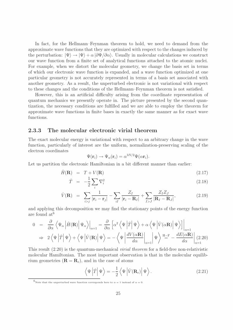
In fact, for the Hellmann–Feynman theorem to hold, we need to demand from theapproximate wave functions that they are optimized with respect to the changes induced bythe perturbation: |Ψ〉 → |Ψ〉+ α |∂Ψ/∂α〉. Usually in molecular calculations we constructour wave function from a finite set of analytical functions attached to the atomic nuclei.For example, when we distort the molecular geometry, we change the basis set in termsof which our electronic wave function is expanded, and a wave function optimized at oneparticular geometry is not accurately represented in terms of a basis set associated withanother geometry. As a result, the unperturbed electronic is not variational with respectto these changes and the conditions of the Hellmann–Feynman theorem is not satisfied.

However, this is an artificial difficulty arising from the coordinate representation ofquantum mechanics we presently operate in. The picture presented by the second quan-tization, the necessary conditions are fulfilled and we are able to employ the theorem forapproximate wave functions in finite bases in exactly the same manner as for exact wavefunctions.

2.3.3 The molecular electronic virial theorem

The exact molecular energy is variational with respect to an arbitrary change in the wavefunction, particularly of interest are the uniform, normalization-preserving scaling of theelectron coordinates

Ψ(ri) → Ψα(ri) = α3N/2Ψ(αri).

Let us partition the electronic Hamiltonian in a bit different manner than earlier:

H(R) = T + V (R) (2.17)

T = −1

2

∑

i

∇2i (2.18)

V (R) =∑

i>j

1

|ri − rj|−∑

iI

ZI

|ri −RI |+∑

I>J

ZIZJ

|RI − RJ |, (2.19)

and applying this decomposition we may find the stationary points of the energy functionare found at6

0 =∂

∂α

⟨

Ψα

∣∣∣H(R)

∣∣∣Ψα

⟩∣∣∣α=1

=∂

∂α

[

α2⟨

Ψ∣∣∣T∣∣∣Ψ⟩

+ α⟨

Ψ∣∣∣V (αR)

∣∣∣Ψ⟩]∣∣∣∣α=1

⇒ 2⟨

Ψ∣∣∣T∣∣∣Ψ⟩

+⟨

Ψ∣∣∣V (R)

∣∣∣Ψ⟩

= −⟨

Ψ

∣∣∣∣

dV (αR)

dα

∣∣∣∣α=1

∣∣∣∣Ψ

⟩

H−F= − dE(αR)

dα

∣∣∣∣α=1

.(2.20)

This result (2.20) is the quantum-mechanical virial theorem for a field-free non-relativisticmolecular Hamiltonian. The most important observation is that in the molecular equilib-rium geometries (R = Re), and in the case of atoms

⟨

Ψ∣∣∣T∣∣∣Ψ⟩

= −1

2

⟨

Ψ∣∣∣V (Re)

∣∣∣Ψ⟩

. (2.21)

6Note that the unperturbed wave function corresponds here to α = 1 instead of α = 0.

25

Furthermore,

⟨

Ψ∣∣∣T∣∣∣Ψ⟩

|R=Re = −E(Re),⟨

Ψ∣∣∣V (Re)

∣∣∣Ψ⟩

= 2E(Re). (2.22)

Also these expressions hold for any approximate wave function that is variational withrespect to a uniform scaling of the nuclear as well as electronic coordinates. Note thataccording to the last result, no stationary points of positive energy may exist.

The scaling force may be easily related to classical Cartesian forces on the nuclei,FI(R) = −dE(R)/dRI , by invoking the chain rule

dE(αR)

dα

∣∣∣∣α=1

=∑

I

d(αRI)

dα

∣∣∣∣α=1

dE(αRI)

d(αRI

∣∣∣∣α=1

= −∑

I

RI · FI(R)

and combining this with virial theorem, we may extract the Cartesian forces experiencedby the nuclei,

∑

I

RI · FI(R) = 2⟨

Ψ∣∣∣T∣∣∣Ψ⟩

+⟨

Ψ∣∣∣V (R)

∣∣∣Ψ⟩

. (2.23)

2.4 One- and N-electron expansions

Let us recall: the Slater determinants do not represent an accurate solution to the molecularSchrodinger equation, but we may express the exact wave function as a superpositionof determinants. Furthermore, it is necessary to expand the molecular orbitals in thedeterminants as a linear combination of atomic orbitals

φa =∑

µ

Cµaχµ(r). (2.24)

As we will see later, atomic orbitals are further approximated with a set of simplerfunctions that are also functions of the coordinates of a single electron. This three-stepprocedure is often referred to as the “standard model of quantum chemistry”. To arriveat the exact solution, i) orbitals in terms of which the determinants are constructed mustform a complete set in one-electron space, and ii) in the expansion of N -electron wavefunction, we must include all determinants that can be generated from these orbitals.

All approximations in the solution of the Schrodinger equation should be unambigiousand precisely defined. Ideally, they should be improvable in a systematic fashion; and toyield more and more elaborate solutions that approach the exact solution. Thus we speakof different models, levels of theory and hierarchies of approximations.

Computational electronic-structure theory has a few standard models for the construc-tion of approximate electronic wave functions. At the simplest level, the wave function isrepresented by a single Slater determinant (the Hartree–Fock approximation); and at themost complex level the wave function is represented as a variationally determined superpo-sition of all determinants in the N -electron Fock space (full configuration-interaction, FCI).

26

Figure 2.2: The two-way hierarchy of approximate molecular wave functions

Between these extremes, there are a vast number of intermediate models with variable costand accuracy.

It should be noted that none of the models is applicable to all systems. However, eachmodel is applicable in a broad range of molecular systems, providing solutions of knownquality and flexibility at a given computational cost.

27

2.5 Further reading

• D. P. Tew, W. Klopper, and T. Helgaker, Electron correlation: the many-body problemat the heart of chemistry, J. Comput. Chem. 28, 1307 (2007)

2.6 Exercises for Chapter 2

1. Here we consider, how the error in the energy can be estimated from the norm of thegradient.

(a) Show that the electronic energy, gradient and Hessian can be expanded arounda stationary point as

E(λ) = E +1

2λTE(2)λ + O(‖λ‖3)

E(1)(λ) = E(2)λ + O(‖λ‖2)

E(2)(λ) = E(2) + O(‖λ‖)

In the above, λ is the vector containing the wave-function parameters; λ = 0

represents the stationary point. E and E(2) are the energy and the Hessian atλ = 0.

(b) Use these expansions to show that the errors in the wave function and in theenergy are related to the gradient as

λ = [E(2)(λ)]−1E(1)(λ) + O(‖E(1)(λ)‖2)

E(λ) − E =1

2[E(1)(λ)]T [E(2)(λ)]−1E(1)(λ) + O(‖E(1)(λ)‖3)

2. ⋆ Consider the uniform scaling of the electron coordinates,

Ψ(ri) → Ψα(ri) = α3N/2Ψ(αri).

Here α is a real scaling factor and N the number of electrons. We assume that Ψ(ri)is normalized.

(a) Shot that the overlap is unaffected by the scaling, i.e.

〈Ψα |Ψα〉 = 1.

(b) Show that the expectation values of the kinetic and potential energies transformas

⟨

Ψα

∣∣∣T∣∣∣Ψα

⟩

= α2⟨

Ψ∣∣∣T∣∣∣Ψ⟩

〈Ψα |V (R)|Ψα〉 = α 〈Ψ |V (αR)|Ψ〉 .

28

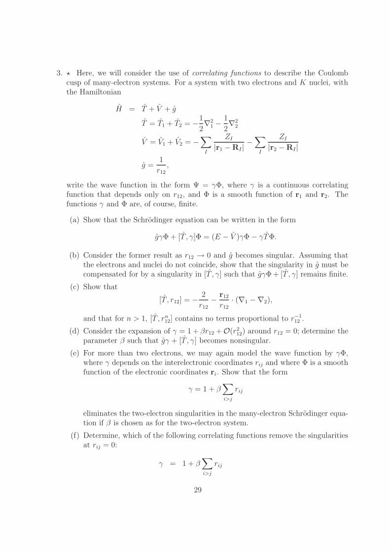
3. ⋆ Here, we will consider the use of correlating functions to describe the Coulombcusp of many-electron systems. For a system with two electrons and K nuclei, withthe Hamiltonian

H = T + V + g

T = T1 + T2 = −1

2∇2

1 −1

2∇2

2

V = V1 + V2 = −∑

I

ZI

|r1 − RI |−∑

I

ZI

|r2 − RI |

g =1

r12,

write the wave function in the form Ψ = γΦ, where γ is a continuous correlatingfunction that depends only on r12, and Φ is a smooth function of r1 and r2. Thefunctions γ and Φ are, of course, finite.

(a) Show that the Schrodinger equation can be written in the form

gγΦ + [T , γ]Φ = (E − V )γΦ − γTΦ.

(b) Consider the former result as r12 → 0 and g becomes singular. Assuming thatthe electrons and nuclei do not coincide, show that the singularity in g must becompensated for by a singularity in [T , γ] such that gγΦ + [T , γ] remains finite.

(c) Show that

[T , r12] = − 2

r12− r12

r12· (∇1 −∇2),

and that for n > 1, [T , rn12] contains no terms proportional to r−1

12 .

(d) Consider the expansion of γ = 1 + βr12 +O(r212) around r12 = 0; determine the

parameter β such that gγ + [T , γ] becomes nonsingular.

(e) For more than two electrons, we may again model the wave function by γΦ,where γ depends on the interelectronic coordinates rij and where Φ is a smoothfunction of the electronic coordinates ri. Show that the form

γ = 1 + β∑

i>j

rij

eliminates the two-electron singularities in the many-electron Schrodinger equa-tion if β is chosen as for the two-electron system.

(f) Determine, which of the following correlating functions remove the singularitiesat rij = 0:

γ = 1 + β∑

i>j

rij

29

γ =∏

i>j

(1 + βrij)

γ = exp

(

β∑

i>j

rij

)

γ = 1 +∑

p

αp exp

(

βp

∑

i>j

r2ij

)

30

Chapter 3

Molecular integral evaluation

3.1 Atomic basis functions

Molecular orbitals can be constructed either numerically or algebraically, of which the for-mer provides greater flexibility and accuracy, but is tractable only for atoms and diatomicmolecules; for polyatomic systems we are forced to expand the MOs φa(r) in a set of somesimple analytical one-electron functions.

Perhaps surprisingly, it turns out that the hydrogenic functions Eq. (1.8) are not idealfor this purpose; as they do not constitute a complete set by themselves but must besupplemented by the unbounded continuum states. Secondly, they become very diffuseand a large number of them is needed for a proper description of both the core and valenceregions of a many-electron atom, especially when located in a molecule.

Therefore, in the molecular electronic-structure theory, χ’s are usually functions ofslightly more unphysical origin. Ideally, they should

1. allow orderly and systematic extension towards completeness with respect to one-electron square-integrable functions

2. allow rapid convergence to any atomic or molecular electronic state, requiring only afew terms for a reasonably accurate description of molecular electronic distributions

3. have an analytical form for easy and accurate manipulation especially for molecularintegrals

4. be orthogonal or at least their non-orthogonality should not pose problems relatedto numerical instability.

Let us begin by reviewing the properties of the hydrogenic functions. As we notedearlier, they are the bounded eigenfunctions of the Hamiltonian

H = −1

2∇2 − Z

r.

31

and are written as

χnlm(r, θ, ϕ) =

(2Z

n

)3/2√

(n− l − 1)!

2n(n + 1)!

(2Zr

n

)l

L2l+1n−l−1

(2Zr

n

)

exp

(

−Zrn

)

︸ ︷︷ ︸

Rnl(r)

×√

2l + 1

4π

(l −m)!

(l +m)!Pm

l (cos θ) exp(imϕ).

︸ ︷︷ ︸

Ylm(θ,ϕ)

The energy of the bounded hydrogenic state χnlm is given by

En = − Z2

2n2. (3.1)

The degeneracy of the hydrogenic states of different angular momenta – that is, 2l + 1degenerate states for every l – is peculiar to the spherical symmetry of the Coulombpotential and is lifted in a many-atom system. The notable features of the radial functionsinclude

• the presence of the exponential

• that Laguerre polynomials introduce n− l − 1 radial nodes in the wave function.

The diffusiveness of χnlm for large n is seen from the expectation value of r

〈χnlm |r|χnlm〉 =3n2 − l(l + 1)

2Z(3.2)

In the following we consider basis functions that retain the product form of the hydrogenicwave functions but have a more compact radial part.

3.1.1 The Laguerre functions

In order to retain the correct exponential behavior but avoid the problems with continuumstates we introduce the following class of functions:

χLFnlm(r, θ, ϕ) = RLF

nl (r)Ylm(θ, ϕ) (3.3)

RLFnl = (2ζ)3/2

√

(n− l − 1)!

(n+ l + 1)!(2ζr)lL2l+2

n−l−1(2ζr) exp(−ζr), (3.4)

referred to as the Laguerre functions. For fixed l and ζ the radial functions (3.4) with n > lconstitute a complete orthonormal set of functions, for which

⟨χLF

nlm |r|χLFnlm

⟩=

2n+ 1

2ζ, (3.5)

32

1050

1s

1050

2s

1050

2p

1050

3s

Figure 3.1: Lagurerre functions.

being thus considerably more compact than the hydrogenic functions for large n and inde-pendent of l. The Laguerre functions exhibit the same nodal structure as the hydrogenicones but their radial distributions R2r2 are quite different (ζ = 1/n, Z = 1).

One should note that the orthogonality of the Laguerre functions is valid only withfixed exponents. It turns out, however, that the expansion of the orbital of a given l-valueof an atomic system requires a large number of fixed-exponent Laguerre functions withdifferent n. For non-orthogonal, variable-exponent functions Laguerre functions are notan optimal choice, but we need to introduce functions specifically tailored to reproduce asclosely as possible the different orbitals of each atom.

3.1.2 Slater-type orbitals

In simplifying the polynomial structure of the Laguerre functions, we note that in RLFnl r

occurs to power l and to powers n− l−1 and lower. Thus a nodeless one-electron functionthat resembles χLF

nlm and the hydrogenic functions closely for large r is obtained by retainingin the Laguerre function only the term of the highest power of r, yielding the Slater-typeorbitals (STO)

χSTOnlm (r, θ, ϕ) = RSTO

nl (r)Y (θ, ϕ) (3.6)

RSTOn (r) =

(2ζ)3/2

√

Γ(2n+ 1)(2ζr)n−1 exp(−ζr) (3.7)

For the STOs we use the same 1s, 2p,... notation as for the hydrogenic functions, keepingin mind that STOs are nodeless and now n only refers to the monomial factor rn−1. Theexpectation value of r and the maximum in the radial distribution curve are given by

⟨χSTO

nlm |r|χSTOnlm

⟩=

2n + 1

2ζ(3.8)

rSTOmax =

n

ζ(3.9)

Also STOs would constitute a complete set of functions for a fixed exponent ζ , and wecould choose to work with a single exponent and include in our basis orbitals (1s, 2s, . . .),(2p, 3p, . . .), (3d, 4d, . . .), all with the same exponent. Alternatively, we may describe theradial space by functions with variable exponents. For each l, we employ only the functions

33

of the lowest n, yielding a basis of the type ((1s(ζ1s), 1s(ζ2s), . . .), (2p(ζ1p, 2p(ζ2p), . . .), . . .)These variable-exponent STOs are given by

χζnllm(r, θ, ϕ) = RSTOζnll

(r)Ylm(θ, ϕ) (3.10)

RSTOζnll

=(2ζnl)

3/2

√

(2l + 2)!(2ζnlr)

l exp(−ζnlr). (3.11)

In practice, a combined approach is employed. For example, for the carbon atom, we wouldintroduce sets of 1s, 2s and 2p functions, all with variable exponents that are chosen toensure an accurate representation of the wave function.

3.1.3 Gaussian-type orbitals

The STO basis sets are very successful for atoms and diatomic molecules, but the evaluationof many-center two-electron integrals becomes very complicated in terms of them. Thebasis sets that have established to be the standard practice in molecular electronic-structuretheory are less connected to the hydrogenic functions or actual charge distributions inmolecules. They are called Gaussian-type orbitals (GTO) as they employ the Gaussiandistributions exp(−αr2) instead of the exp(−ζr) as in STOs. A large number of GTOs areneeded to describe an STO (or an AO) properly, but this is more than compensated by afast evaluation of the molecular integrals.

The spherical-harmonic GTOs are

χGTOnlm (r, θ, ϕ) = RGTO

nl (r)Ylm(θ, ϕ) (3.12)

RGTOnl (r) =

2(2α)3/4

π1/4

√

22n−l−2

(4n− 2l − 3)!!(√

2αr)2n−l−2 exp(−αr2). (3.13)

They form a complete set of nonorthogonal basis functions. In above, the double factorialfunction is

n!! =

1 n = 0n(n− 2)(n− 4) · · ·2 even n > 0n(n− 2)(n− 4) · · ·1 oddn > 0

1(n+2)(n+4)···1

oddn < 0

(3.14)

The spatial extent of the GTOs are

⟨χGTO

nlm |r|χGTOnlm

⟩≈

√

2n− l − 2

2α(3.15)

rGTOmax =

√

2n− l − 1

2α(3.16)

When we compare these results with the case of STOs, we note that much larger numberof GTOs are needed for a flexible description of outer regions of the electron distribution.

34

0.0

2.5

0 1 2 3 4 5

1s STO (ζ=1)2s STO (ζ=1)

0.0

2.5

5.0

0 1 2 3 4 5

1s GTO (α=1)2s GTO (α=1)2p GTO (α=1)

0.0

2.5

5.0

0 1 2 3 4 5

1sSTO (ζ=1)GTO (α=1)

0.0

2.5

5.0

7.5

0 1 2 3 4 5

1sGTO (α=3.42)GTO (α=0.62)GTO (α=0.16)

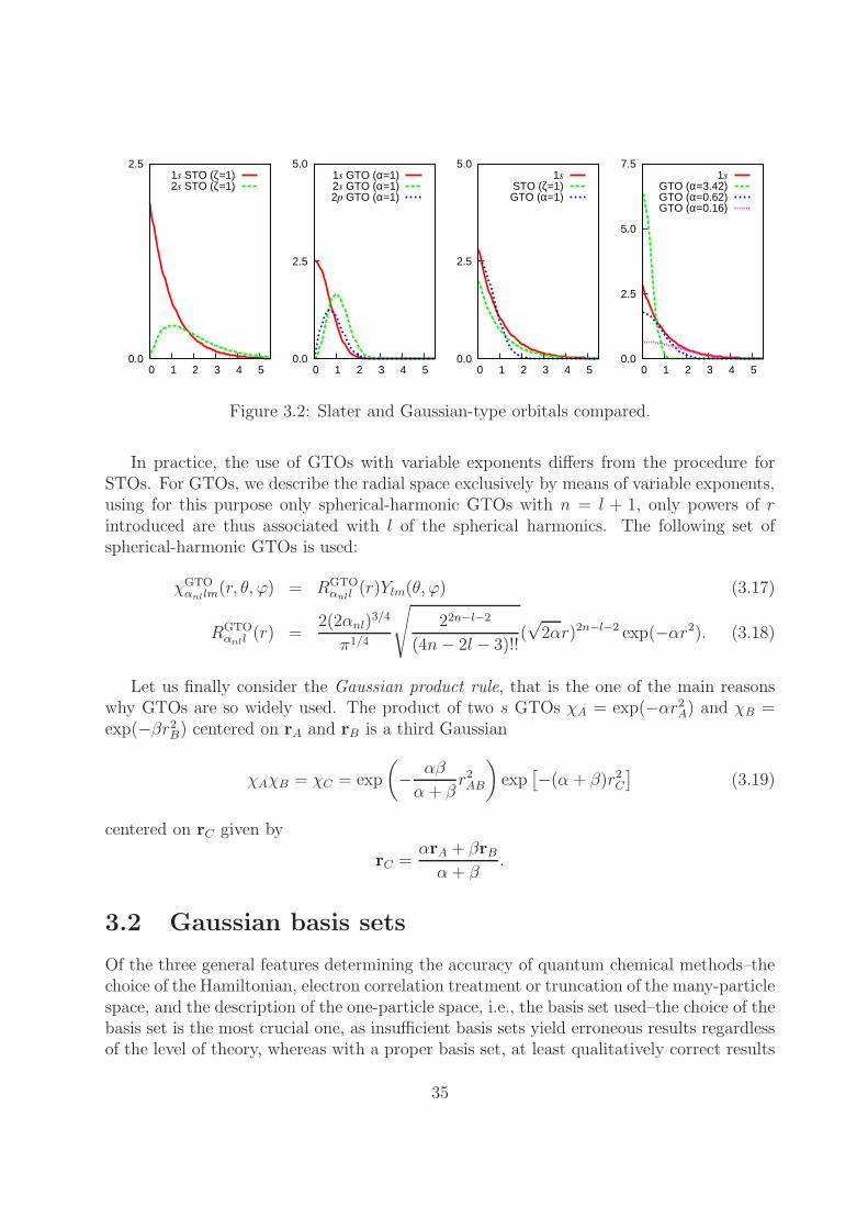
Figure 3.2: Slater and Gaussian-type orbitals compared.

In practice, the use of GTOs with variable exponents differs from the procedure forSTOs. For GTOs, we describe the radial space exclusively by means of variable exponents,using for this purpose only spherical-harmonic GTOs with n = l + 1, only powers of rintroduced are thus associated with l of the spherical harmonics. The following set ofspherical-harmonic GTOs is used:

χGTOαnllm

(r, θ, ϕ) = RGTOαnll

(r)Ylm(θ, ϕ) (3.17)

RGTOαnll

(r) =2(2αnl)

3/4

π1/4

√

22n−l−2

(4n− 2l − 3)!!(√

2αr)2n−l−2 exp(−αr2). (3.18)

Let us finally consider the Gaussian product rule, that is the one of the main reasonswhy GTOs are so widely used. The product of two s GTOs χA = exp(−αr2

A) and χB =exp(−βr2

B) centered on rA and rB is a third Gaussian

χAχB = χC = exp

(

− αβ

α + βr2AB

)

exp[−(α + β)r2

C

](3.19)

centered on rC given by

rC =αrA + βrB

α + β.

3.2 Gaussian basis sets

Of the three general features determining the accuracy of quantum chemical methods–thechoice of the Hamiltonian, electron correlation treatment or truncation of the many-particlespace, and the description of the one-particle space, i.e., the basis set used–the choice of thebasis set is the most crucial one, as insufficient basis sets yield erroneous results regardlessof the level of theory, whereas with a proper basis set, at least qualitatively correct results

35

can be obtained for many problems already at the uncorrelated level of theory and usingthe non-relativistic Hamiltonian.

The majority of quantum chemical applications employ contracted GTO (CGTO) sets,i.e. linear combinations of GTO functions with coefficients optimized regarding somecriterion (usually SCF energy) that significantly increase efficiency. There are two widelyused contraction schemes: segmented contraction, where each GTO contributes only to asingle CGTO, and general contraction, where such a restriction is not applied. Examples ofthe segmented scheme include the Pople-style basis set families (3-21G, 6-31G,...) and theKarlsruhe basis sets. The correlation-consistent (cc) basis set families by Dunning and co-workers are the most widely used generally contracted basis sets. The basic idea behind thecc sets is that functions that contribute approximately the same amount to the correlationenergy are added to the basis in groups. The cc basis sets provide smooth, monotonicconvergence for the electronic energy as well as for many molecular properties, especiallythose originating in the valence region. The polarized valence (cc-pVXZ, X = D, T, Q, 5,6 corresponding to the number of CGTOs used to represent an occupied atomic orbital)and core-valence (cc-pCVXZ) sets can be augmented with diffuse functions (aug-cc-pVXZand aug-cc-pCVXZ; d-aug-cc-pVXZ and t-aug-cc-pVXZ for doubly and triply augmentedsets, respectively). While these features are favorable and the sets are widely used, the cc-basis sets become very large at large X, and it is not straightforward to extend the familybeyond the published X values or to new elements. The atomic natural orbital (ANO) basissets provide another general contraction approach. The contraction coefficients therein areatomic ANO coefficients that are obtained by optimizing atomic energies.

The use of increasingly large basis sets that produce results converging to some partic-ular value is usually regarded as a solution to the problem of basis set incompleteness. Incalculations of molecular properties that originate, e.g., in the region close to the nuclei(examples include indirect spin-spin couplings and hyperfine couplings), approaching thebasis-set limit using the cc or comparable energy-optimized paradigms may lead to exces-sively large basis sets prohibiting calculations of large molecules. An alternative and oftenused approach is to uncontract the basis set and to supplement it by additional steep basisfunctions in the l-shells relevant for the property under examination.

The performance of the different basis sets for a certain molecular property can bequalitatively understood within a concept, which can be measured by the completenessprofiles

Y(α) =∑

m

〈g(α)|χm〉2. (3.20)

Here χ denotes a set of orthonormalized, contracted or primitive, basis functions, andg(α) is a primitive “test” GTO with the exponent α, used to probe the completeness ofχ. The completeness profile becomes unity for all α, for all l-values in a CBS. Y(α)is typically plotted in the logarithmic scale, against x = logα. In a certain exponentinterval [αmin, αmax] this quantity is intuitively connected to the possibility – from thepoint of view of one-particle space – of describing all details of the wave function in thecorresponding distance range from the atomic nuclei. Put simply, atomic properties that

36

1.0

0.75

0.5

0.25

Y(α

)

(a) spd

(b) spdf

1.0

0.75

0.5

0.25

Y(α

)

(c) spdfg

(d)spdfgh

1.0

0.75

0.5

0.25

Y(α

)

(e)spdfghi

(f)spdf

1.0

0.75

0.5

0.25

-4-3-2-101234

Y(α

)

Log (α)

(g)spdf

-4-3-2-101234Log (α)

(h)spdf

Figure 3.3: Completeness profiles of (a) cc-pVDZ (b) cc-pVTZ (c) cc-pVQZ (d) cc-pV5Z(e) cc-pV6Z (f) cc-pCVTZ (g) aug-cc-pVTZ and (h) aug-cc-pCVTZ basis sets of fluorine.

obtain relevant contributions roughly within [1/√αmax, 1/

√αmin] from the nucleus can be

reproduced by a basis that has Y(α) = 1 in this interval. This way of thinking can begeneralized to molecular properties that may be dominated by phenomena occurring closeto the expansion centers of the basis functions, i.e., atomic nuclei (region described byhigh-exponent basis functions) and/or in the valence region, further away from the nuclei.

3.3 Integrals over Gaussian basis sets

In the following, we will evaluate the one- and two-electron integrals

Oµν = 〈χµ

∣∣∣O⟩

χν =

∫

drχµ(r)O(r)χν(r) (3.21)

37

Oµνλσ = 〈χµ(1)χν(1)∣∣∣O⟩

χλ(2)χσ(2)

=

∫

dr1dr2χµ(r1)χν(r1)O(r)χλ(r2)χσ(r2) (3.22)

such that the AOs (χ) are taken as fixed linear combinations of real-valued primitiveCartesian GTOs

Gijk(r, a,R) = xiRy

jRz

kR exp(−ar2

R), (3.23)

where the ”Cartesian quantum numbers” i, j, k are greater than zero and l = i+ j+ k fora given total angular momentum quantum number.

The integrals over primitive Cartesian GTOs may subsequently be transformed to in-tegrals over contracted and/or spherical-harmonic GTOs by linear combinations.

3.3.1 Gaussian overlap distributions

An important property of the primitive Cartesian GTOs is that they can be factorized inthe three Cartesian directions,

Gijk(r, a, R) = Gi(x, a, Rx)Gj(y, a, Ry)Gz(z, a, Rz), (3.24)

where for example Gi(x, a, Rx) = xiR exp(−ax2

R). We will need also a concept of Gaussianoverlap distribution

Ωab(r) = Gijk(r, a,RA)Glmn(r, b,RB), (3.25)

that may also be factorized in the same way

Ωab(r) = Ωxij(x, a, b, RA,x, RB,x)Ω

ykl(y, a, b, RA,y, RB,y)Ω

zmn(z, a, b, RA,z, RB,z), (3.26)

where the x component (for example) is given by

Ωxij(x, a, b, RA,x, RB,x) = Gi(x, a, RA,x)Gj(x, b, RB,x). (3.27)

3.3.2 Simple one-electron integrals

We are now ready to consider simple one-electron integrals, by which we mean molecularintegrals that do not involve the singular Coulombic 1/r interaction. All such integrals canbe factorized in the three directions as

Sab = SijSklSmn. (3.28)

According to the Gaussian product rule (3.19), any Cartesian component of the overlapdistribution can be written as a single Gaussian at the centre of charge Px, and we maythus evaluate the integral

∫ ∞

−∞

Ωx00dx = exp(−µX2

AB)

∫ ∞

−∞

exp(−px2p)dx =

√π

pexp(−µX2

AB), (3.29)

38

where µ denotes the reduced exponent ab/(a + b), p = a+ b, and

Px =aRA,x + bRB,x

p(3.30)

XAB = RA,x −RB,x. (3.31)

This result provides a basis for a set of recurrence relations by which we may evaluatesimple integrals – overlap or more complicated ones – over GTOs of arbitrary quantumnumbers. This procedure is known as Obara–Saika scheme. There exist other methodsfor molecular integral evaluation but we will not discuss them here. The relations areobtained by considering the behaviour of the integral under coordinate transformation andtheir detailed derivation is omitted here but recommended further reading.

The simplest case is the overlap integral

Sab = 〈Ga |Gb〉 , (3.32)

for an Cartesian component of which the Obara–Saika relations are written as

Si+1,j = XPASij +1

2p(iSi−1,j + jSi,j−1) (3.33)

Si,j+1 = XPBSij +1

2p(iSi−1,j + jSi,j−1). (3.34)

For the linear and angular momentum as well as for kinetic energy integrals we needthe integrals over differential operators

Defgab =

⟨

Ga

∣∣∣∣

∂e

∂xe

∂f

∂yf

∂g

∂zg

∣∣∣∣Gb

⟩

. (3.35)

In one direction the relations are

Dei+1,j = XPAD

eij +

1

2p(iDe

i−1,j + jDei,j−1 − 2beDe−1

ij ) (3.36)

Dei+1,j = XPBD

eij +

1

2p(iDe

i−1,j + jDei,j−1 + 2aeDe−1

ij ), (3.37)

with the e = 0 case providing the starting point and being equivalent with the overlapintegral.

3.3.3 The Boys function

We will now introduce a special function that has a key role in the evaluation of one- andtwo-electron Coulomb integrals, the Boys function of order n, defined as

Fn(x) =

∫ 1

0

exp(−xt2)t2ndt. (3.38)

39

2 4 6 8 10

0.2

0.4

0.6

0.8

1

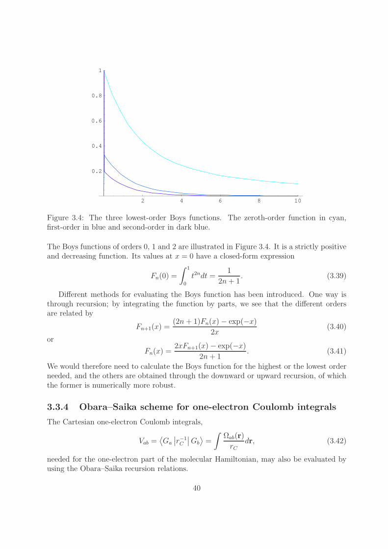
Figure 3.4: The three lowest-order Boys functions. The zeroth-order function in cyan,first-order in blue and second-order in dark blue.

The Boys functions of orders 0, 1 and 2 are illustrated in Figure 3.4. It is a strictly positiveand decreasing function. Its values at x = 0 have a closed-form expression

Fn(0) =

∫ 1

0

t2ndt =1

2n+ 1. (3.39)

Different methods for evaluating the Boys function has been introduced. One way isthrough recursion; by integrating the function by parts, we see that the different ordersare related by

Fn+1(x) =(2n + 1)Fn(x) − exp(−x)

2x(3.40)

or

Fn(x) =2xFn+1(x) − exp(−x)

2n+ 1. (3.41)

We would therefore need to calculate the Boys function for the highest or the lowest orderneeded, and the others are obtained through the downward or upward recursion, of whichthe former is numerically more robust.

3.3.4 Obara–Saika scheme for one-electron Coulomb integrals

The Cartesian one-electron Coulomb integrals,

Vab =⟨Ga

∣∣r−1

C

∣∣Gb

⟩=

∫Ωab(r)

rC

dr, (3.42)

needed for the one-electron part of the molecular Hamiltonian, may also be evaluated byusing the Obara–Saika recursion relations.

40

We again factorize the distribution according to (3.26), and are about to obtain theintegrals through the recursion relations (c.f., below) for auxillary integrals ΘN

ijklmn:

ΘNi+1 jklmn = XPAΘN

ijklmn +1

2p(iΘN

i−1 jklmn + jΘNi j−1 klmn)

−XPCΘN+1ijklmn − 1

2p(iΘN+1

i−1 jklmn + jΘN+1i j−1klmn) (3.43)

ΘNi j+1klmn = XPBΘN

ijklmn +1

2p(iΘN

i−1 jklmn + jΘNi j−1klmn)

−XPCΘN+1ijklmn − 1

2p(iΘN+1

i−1 jklmn + jΘN+1i j−1klmn) (3.44)

with the special cases (that also serve the starting points of the recursion)

Θ0ijklmn = Vijklmn = Vab (3.45)

ΘN000000 =

2π

pKxyz

ab FN(pR2PC), (3.46)

where FN is the Boys function, and we have denoted

Kxab = exp(−µX2

AB). (3.47)

3.3.5 Obara–Saika scheme for two-electron Coulomb integrals

The evaluation of electron-electron repulsion integrals is a highly non-trivial task and dueto their bottleneck status, under intense study since the early days of quantum chemistry.We will discuss here only one of the numerous schemes that is in accordance with theearlier discussion, namely the Obara–Saika scheme for Cartesian two-electron integrals,

gabcd =⟨Ga(r1)Gb(r1)

∣∣r−1

12

∣∣Gc(r2)Gd(r2)

⟩=

∫ ∫Ωab(r1)Ωcd(r2)

r12dr1dr2. (3.48)

The relations feature similarly to the one-electron corresponds a set of auxillary integralsΘ. Again, two special cases of them are required:

ΘN0000 0000 0000 =

2π5/2

pq√p+ q

Kxyzab Kxyz

cd FN(αR2PQ) (3.49)

Θ0ixjxkxlx iyjykyly izjzkzlz = gixjxkxlx iyjykyly izjzkzlz = gabcd. (3.50)

In the above, we have denoted Kxyzab = Kx

abKyabK

zab [c.f. Eq. (3.47)] and α is the reduced

exponent pq/(p + q). FN is again the Boys function. In the following, the indices i, j,k and l are the Cartesian quantum numbers for orbitals a, b, c and d in the x-direction.Starting from these, first a set of integrals with j = k = l = 0 is generated by

Θi+1000 = XPAΘNi000 −

α

pXPQΘN+1

i000 +i

2p

(

ΘNi−1 000 −

α

pΘN+1

i−1 000

)

. (3.51)

41

Then, the second electron is treated using the integrals generated in (3.51):

Θi0 k+10 = −bXAB + dXCD

qΘN

i0k0 −i

2qΘN

i−1 0k0 +k

2qΘN

i0 k−1 0 −p

qΘN

i+10k0. (3.52)

In the final step, the Cartesian powers are ”transferred” between the orbitals of the sameelectron:

Θi j+1kl = Θi+1 jkl +XABΘNijkl (3.53)

Θijkl+1 = Θij k+1 l +XCDΘNijkl. (3.54)

In this way, we may construct the full set of Cartesian two-electron Coulomb integrals.

42

3.4 Further reading

• T. Helgaker and P. Taylor, Gaussian basis sets and molecular integrals, in ModernElectronic Structure Theory, Part II, D. R. Yarkony (ed.), (World Scientific 1995),pp. 725–856

• R. Lindh, Integrals of electron repulsion, in P. v. R. Schleyer et al. (eds.), Encyclo-pedia of Computational Chemistry Vol. 2, (Wiley 1998) p. 1337.

• M. C. Strain, G. E. Scuseria and M. J. Frisch, Achieving linear scaling for the elec-tronic quantum Coulomb problem, Science 271, 51 (1996).

• S. Obara and M. Saika, Efficient recursive computation of molecular integrals overCartesian Gaussian functions, Journal of Chemical Physics 84, 3963 (1986); 89, 1540(1988).

3.5 Exercises for Chapter 3

1. Verify the expressions for radial extents

〈r〉 =

∫ ∞

0

Rnl(r)rRnl(r)r2dr

of (a) the hydrogenic wave functions, (b) the Laguerre functions, (c) the radial STOs.

2. ⋆ In this exercise, we study the radial form of the GTOs, the most frequently usedbasis functions in molecular electronic-structure theory:

RGTOαl (r) = NGTO

αl (√

2αr)l exp(−αr2).

The related functions RGTOnl are obtained by replacing l by 2n− l − 2.

(a) Using the integral

∫ ∞

0

x2n exp(−αx2)dx =(2n− 1)!!

2n+1

√π

α2n+1, n ≥ 0, α > 0

verify that the normalization constant NGTOαl is given by

NGTOαl =

2(2α)3/4

π3/4

√

2l

(2l + 1)!!.

(b) Determine the radial overlap between two GTOs:

Sα1α2l =

∫ ∞

0

RGTOα1l (r)RGTO

α2l (r)r2dr.

43

(c) By setting α2 = βα1 verify that the overlap Sα1 βα1 l is independent of α1.

(d) Using the integral

∫ ∞

0

x2n+1 exp(−αx2)dx =n!

2αn+1n ≥ 0, α > 0

show that the expectation value of r is

〈r〉 =

∫ ∞

0

RGTOαl (r)rRGTO

αl (r)r2dr =

√

2

πα

2l(l + 1)!

(2l + 1)!!.

(e) Use the Stirling approximation for factorials k! ∼ kk+1/2√

2πe−k (k ≫ 1) toshow that 〈r〉 is for large l

〈r〉 ∼√

l

2α.

(f) Verify that the radial distribution function 4πr2[RGTOαl (r)]2 has a maximum at

rGTOmax =

√

l + 1

2α.

(g) Consider two GTOs of different l and exponents. Determine the relation betweenα1 and α2 so that the radial distribution of these GTOs have the same maximum.

3. Using the Obara–Saika scheme, evaluate the self-overlap integrals 〈px |px〉 and 〈dx2 |dx2〉.

4. Construct the Obara–Saika recursion relations for kinetic-energy integrals

Tab = −1

2

⟨Ga

∣∣∇2∣∣Gb

⟩.

5. ⋆ Derive the Obara–Saika relations for overlap and differential operator integrals,Eqs. (3.33-3.34) and (3.36-3.37).

44

Chapter 4

Second quantization

4.1 Fock space

We now introduce an abstract linear vector space – the Fock space – where each Slaterdeterminant (1.20) of M orthonormal spin-orbitals is represented by an occupation numbervector (ON) k,

|k〉 = |k1, k2, . . . , kM〉 , kP =

1 ψP occupied0 ψP unoccupied

(4.1)

For an orthonormal set of spin-orbitals, we define the inner product between two ON vectorsas

〈m |k〉 =M∏

P=1

δmP kP. (4.2)

This definition is consistent with the overlap between two Slater determinants, but has awell-defined but zero overlap between states with different electron numbers is a specialfeature of the Fock-space formulation. It allows for a unified description of systems withvariable numbers of electrons.

• In a given spin-orbital basis, there is a one-to-one mapping between the Slater de-terminants with spin-orbitals in a canonical order and the ON vectors in the Fockspace.

• However, ON vectors are not Slater determinants: ON vectors have no spatial struc-ture but are just basis vectors in an abstract vector space.

• The Fock space can be manipulated as an ordinary inner-product vector space.

The ON vectors constitute an orthonormal basis in the 2M dimensional Fock spaceF (M), that can be decomposed as a direct sum of subspaces,

F (M) = F (M, 0) ⊕ F (M, 1) ⊕ · · · ⊕ F (M,N), (4.3)

45

where F (M,N) contains all ON vectors obtained by distributing N electrons among theM spin-orbitals, in other words, all ON vectors for which the sum of occupation numberis N . The subspace F (M, 0) is the vacuum state,

|vac〉 = |01, 02, . . . , 0M〉 . (4.4)

Approximations to an exact N -electron wave function are expressed in terms of vectors in

the Fock subspace F (M,N) of dimension equal to

(MN

)

.

4.1.1 Creation and annihilation operators

In second quantization, all operators and states can be constructed from a set of elementarycreation and annihilation operators. The M creation operators are defined by

a†P |k1, k2, . . . , 0P , . . . , kM〉 = Γk

P |k1, k2, . . . , 1P , . . . , kM〉 (4.5)

a†P |k1, k2, . . . , 1P , . . . , kM〉 = 0 (4.6)

where

Γk

P =P−1∏

Q=1

(−1)kQ. (4.7)

The definition can be also combined a single equation:

a†P |k1, k2, . . . , 0P , . . . , kM〉 = δkP 0Γk

P |k1, k2, . . . , 1P , . . . , kM〉 (4.8)

Operating twice with a†P on an ON vector gives

a†Pa†P |k1, k2, . . . , 0P , . . . , kM〉 = a†P δkP 0Γ

k

P |k1, k2, . . . , 1P , . . . , kM〉 = 0,

thereforea†Pa

†P = 0. (4.9)

For Q > P ,

a†Pa†Q |. . . , kP , . . . , kQ, . . .〉 = a†P δkQ0Γ

k

Q |. . . , kP , . . . , 1Q, . . .〉= δkP 0δkQ0Γ

k

P Γk

Q |. . . , 1P , . . . , 1Q, . . .〉 .

Reversing the order of the operators,

a†Qa†P |. . . , kP , . . . , kQ, . . .〉 = a†QδkP 0Γ

k

P |. . . , 1P , . . . , kQ, . . .〉= δkP 0δkQ0Γ

k

P (−Γk

Q) |. . . , 1P , . . . , 1Q, . . .〉 .

and combining the results, we obtain

a†Pa†Q + a†Qa

†P |k〉 = 0.

46

Substitution of dummy indices shows that this holds for Q < P as well, and is true alsofor Q = P . Since |k〉 is an arbitrary ON vector, we conclude the anticommutation relation

a†Pa†Q + a†Qa

†P = [a†P , a

†Q]+ = 0. (4.10)

The properties of the adjoint or conjugate operators aP can be reasoned from those ofthe creation operators. Thus, the adjoint operators satisfy the anticommutation relation

[aP , aQ]+ = 0. (4.11)

Let us invoke the resolution of the identity:

aP |k〉 =∑

m

|m〉 〈m |aP |k〉 ,

where, using Eq. (4.8),

〈m |aP |k〉 = 〈k |aP |m〉∗ =

δmP 0Γ

m

P if kQ = mQ + δQP

0 otherwise.

From the definition of Γ and from kQ = mQ + δQP we see that ΓmP = ΓK

P . We may thereforewrite the equation as

〈m |aP |k〉 =

δkP 1Γ

k

P ifmQ = kQ − δQP

0 otherwise.

Hence, only one term in aP |k〉 survives:

aP |k〉 = δkP 1Γk

P |k1, . . . , 0P , . . . , kM〉 . (4.12)

The operator aP is called the annihilation operator.Combining Eqs. (4.8) and (4.12), we get

a†PaP |k〉 = δkP 1 |k〉 (4.13)

aPa†P |k〉 = δkP 0 |k〉 (4.14)

that leads toa†PaP + aPa

†P = 1. (4.15)

For P > Q, we have

a†PaQ |k〉 = −δkP 0δkQ1Γk

P Γk

Q |k1, . . . , 0Q, . . . , 1P , . . . , kM〉aQa

†P |k〉 = δkP 0δkQ1Γ

k

PΓk

Q |k1, . . . , 0Q, . . . , 1P , . . . , kM〉 ,

thus we have the operator identity

a†PaQ + aQa†P = 0 P > Q. (4.16)

Hence,a†PaQ + aQa

†P = [a†P , aQ]+ = δPQ. (4.17)

47

4.1.2 Number-conserving operators

The occupation-number operator that counts the number of electrons in spin-orbital P isintroduced as

NP = a†PaP , NP |k〉 = kP |k〉 (4.18)

The occupation-number operators are Hermitian, N † = N , as well as idempotent, N2P =

NP . Using the basic anticommutation relations, we obtain

[NP , a†Q] = δPQa

†Q (4.19)

[

NP , aQ

]

= −δPQaQ (4.20)

So for an arbitrary string X consisting of creation and annihilation operators, e.g. X =a†PaQaPa

†RaS, the commutators with N become

[NP , X] = NXP X, (4.21)

where NXP is the number of times a†P occurs in X minus the number of times aP occurs.

All occupation-number operators added together in the Fock space gives the Hermitianoperator

N =M∑

P=1

a†PaP , (4.22)

which returns the number of electrons in an ON vector, N |k〉 = N |k〉, and is thereforeknown as the particle-number operator. We find that the number operator commutes withany string T that contains an equal number of creation and annihilation operators. Suchstrings are called number-conserving. In general, the application of the string X to aFock-space vector increases the number of electrons by NX .

The simplest number-conserving operators are the elementary excitation operators

EPQ = a†PaQ, (4.23)

which give as applied to an ON vector

a†PaQ |k〉 = a†P δkQ1Γk

Q |k1, . . . , 0Q, . . . , kP , . . . , kM〉= δkP 0δkQ1Γ

k

QΓk

P εPQ |k1, . . . , 0Q, . . . , 1P , . . . , kM〉

= εPQΓk

QΓk

P (1 − kP )kQ

∣∣∣∣

kP → 1kQ → 0

⟩

(4.24)

where

εPQ =

1 P ≤ Q−1 P > Q

.

The case P < Q differs from this result only in the interpretation of εPQ, whereas the caseP = Q is covered by Eq. (4.18). Therefore we may write

a†PaQ |k〉 = εPQΓk

P Γk

Q(1 − kP + δPQ)kQ

∣∣∣∣

kP → 1kQ → δPQ

⟩

. (4.25)

48

First quantization Second quantization

• One-electron operator:

f c =

N∑

i=1

f(xi)

• One-electron operator:

f =∑

PQ

fPQa†PaQ

• Two-electron operator:

gc =N∑

i=1

N∑

j=i+1

g(xi,xj)

• Two-electron operator:

g =1

2

∑

PQRS

gPQRSa†Pa

†RaSaQ

• Operators are independent of the spin-orbital basis

• Operators depend on the spin-orbital ba-sis

• Operators depend on the number of elec-trons

• Operators are independent of electrons

• Operators are exact • Projected operators

Table 4.1: Comparison between first and second quantization representations.

The application of a single such operator gives a single excitation, two a double excitationand so forth.

4.2 The representation of one- and two-electron op-

erators

Expectation values of Hermitian operators correspond to physical observables and shouldthus be independent of the representation of operators and states. Therefore, we requirethe matrix element of a second-quantization operator between two ON vectors to be equalto its first-quantization counterpart.

To determine the numerical parameters fPQ in the second-quantization representation

of one-electron operators, we evaluate the matrix elements of f between two ON vectorsand compare with the usual Slater rules for matrix elements between determinants. Weare lead to the identification

fPQ =⟨

ψP

∣∣∣f c∣∣∣ψQ

⟩

(4.26)

gPQRS = 〈ψPψR |gc|ψQψS〉 . (4.27)

The parameters gPQRS possess the particle-interchange symmetry,

gPQRS = gRSPQ. (4.28)

49

In the case of real spin-orbitals, the integrals exhibit the following permutational symme-tries:

fPQ = fQP (4.29)

gPQRS = gQPRS = gPQSR = gQPSR, (4.30)

of which the latter may be further combined with Eq. (4.28) to yield an eight-fold symmetry.Using the introduced second-quantization representation, we may now construct the

(non-relativistic, spin-free) molecular electronic Hamiltonian in the Born–Oppenheimerapproximation,

H =∑

PQ

hPQa†PaQ +

1

2gPQRSa

†Pa

†RaSaQ + hnuc, (4.31)

where

hPQ =

∫

ψ∗P (x)

(

−1

2∇2 −

∑

I

ZI

riI

)

ψQ(x)dx (4.32)

gPQRS =

∫ψ∗

P (x)ψ∗R(x)ψQ(x)ψS(x)

r12dx1dx2 (4.33)

hnuc =1

2

∑

I 6=J

ZIZJ

RIJ

. (4.34)

The form of the second-quantization Hamiltonian can be interpreted in the following way:Applied to an electronic state, the Hamiltonian produces a linear combination of the orig-inal state with states generated by single and double electron excitations from this state.With each such excitation, there is an associated amplitude hPQ or gPQRS, which representsthe probability of this event happening.

Let Ac, Bc and Cc be one-electron operators in first quantization and A, B and C bethe corresponding second-quantization representations.

• The first-quantization operator aAc + bBc, where a and b are numbers, is representedby aA + bB.

• The standard relations

A(BC) = (AB)C (4.35)

(AB)† = B†A† (4.36)

are valid.

• For a complete one-electron basis

Cc = AcBc ⇒ C = AB

but for finite basis sets this expression does not hold. The second-quantization op-erators are projections of the exact operators onto a basis of spin-orbitals. For anincomplete basis, the second-quantization representation of an operator product de-pends on when the projection is made.

50

Second quantization treats operators and wave functions in a unified way – they are allexpressed in terms of the elementary creation and annihilation operators: any ON vectormay be written as

|k〉 = Xk |vac〉 =

[M∏

P=1

(a†P )kP

]

|vac〉 (4.37)

and therefore the matrix elements can be viewed as the vacuum expectation value of anoperator

⟨

k

∣∣∣O∣∣∣m⟩

=⟨

vac∣∣∣X

†kOXm

∣∣∣ vac

⟩

, (4.38)

and expectation values become linear combinations of vacuum expectation values.

4.3 Commutators and anticommutators

In the manipulation of operators and matrix elements in second quantization, the commu-tator [A, B] = AB− BA and the anticommutator [A, B]+ = AB+ BA of two operators areoften encountered. Referring to the basic relations of the elementary creation and annihi-lation operators, it is usually possible to simplify the commutators and anticommutatorsbetween strings of elementary operators considerably.

We need to introduce the concepts of operator rank and rank reduction.

• The (particle) rank of a string of creation and annihilation operators is simply thenumber of elementary operators divided by 2.

• Rank reduction is said to occur when the rank of a commutator or anticommutatoris lower than the combined rank of the operators commuted or anticommuted.

A simple rule

• Rank reduction follows upon anticommutation of two strings of half-integral rankand upon commutation of all other strings

is useful for simplifying the expressions.One useful strategy for the evaluation of commutators and anticommutators is based

on their linear expansion in simpler commutators or anticommutators according to e.g. thefollowing operator identities (see Exercise 3), and aim at greatest possible rank reduction:

[

A, B1B2

]

= [A, B1]B2 + B1[A, B2] (4.39)

[

A, B1 · · · Bn

]

=n∑

k=1

B1 · · · Bk−1[A, Bk]Bk+1 · · · Bn (4.40)

[

A, B1B2

]

= [A, B1]+B2 − B1[A, B2]+ (4.41)

51

[

A, B1 · · · Bn

]

=

n∑

k=1

(−1)k−1B1 · · · [A, Bk]+ · · · Bn (n even) (4.42)

[

A, B1B2

]

+= [A, B1]B2 + B1[A, B2]+ = [A, B1]+B2 − B1[A, B2] (4.43)

[

A, B1 · · · Bn

]

+=

n∑

k=1

(−1)k−1B1 · · · [A, Bk]+ · · · Bn (n odd). (4.44)

4.3.1 Evaluation of commutators and anti-commutators

Let us consider the simplest nontrivial commutator, [a†P , a†QaR]. Moving one of the opera-

tors after the comma out of the commutators by using (4.41),

[a†P , a†QaR] = [a†P , a

†Q]+aR − a†Q[a†P , aR]+ (4.45)

and invoking the basic anticommutation relation we have

[a†P , a†QaR] = −δPRa

†Q. (4.46)

Similarly,

[aP , a†QaR] = δPQaR. (4.47)

Then, let us evaluate the commutator between two excitation operators, using theresults from the previous example,

[a†PaQ, a†RaS] = [a†P , a

†Ra

†S]aR + a†P [aQ, a

†RaS] = δQRa

†PaS − δPSa

†RaQ. (4.48)

A slightly more complicated commutator is evaluated by applying Eq. (4.39) and theprevious result:

[a†PaQ, a†RaSa

†MaN ] = [a†PaQ, a

†RaS]a†MaN + a†RaS[a†PaQ, a

†MaN ]

= δQRa†PaSa

†MaN − δPSa

†RaQa

†MaN

+δQMa†RaSa

†PaN − δPNa

†RaSa

†MaQ. (4.49)

The following double commutator can be evaluated by invoking the result (4.48) twice

[a†PaQ, [a†RaS, a

†MaN ]] = δSM [a†PaQ, a

†Ra

†N ] − δRN [a†PaQ, a

†MaS]

= δSMδQRa†PaN − δSMδPMa

†RaQ − δRNδQMa

†PaS

+δRNδPSa†MaQ. (4.50)

This gives rise to a rank reduction by 2.

52

4.4 Orbital rotations

In many situations, e.g., during the optimization of an approximate electronic state or inthe calculation of the response of an electronic state to an external perturbation, it becomesnecessary to carry out transformations between different sets of orthonormal spin-orbitals.

We shall encounter especially cases where the occupation numbers refer to a set oforthonormal spin-orbitals ψP that is obtained from another set ψP by a unitary transfor-mation

ψP =∑

Q

ψQUQP . (4.51)

Here, a unitary matrix U is a matrix that fulfills the relation

U†U = UU† = 1. (4.52)

The spectral theorem states that any unitary matrix can be diagonalized as

U = VǫV†,

where V is unitary and ǫ a complex diagonal matrix, ǫkk = exp(iδk). Therefore any unitarymatrix can be written as the matrix exponential1 of an anti-Hermitian matrix:

U = V exp(iδ)V† = exp(iVδV†)

≡ exp(X), X = −X†. (4.53)

By an introduction of the anti-Hermitian operator

κ =∑

PQ

κPQa†PaQ, κ† = −κ, (4.54)

where the parameters κPQ are the elements of an anti-Hermitian matrix κ, for which

U = exp(−κ), the elementary operators a†P , aP and state∣∣0⟩

generated by the unitarytransformation (4.51) can be expressed in terms of the untransformed operators and statesas

a†P = exp(−κ)a†P exp(κ) (4.55)

aP = exp(−κ)aP exp(κ) (4.56)∣∣0⟩

= exp(−κ) |0〉 . (4.57)

4.5 Spin in second quantization

In the formalism of second quantization, there is no reference to electron spin. However,in non-relativistic theory, many important simplifications follow by taking spin explicitly

1The matrix exponential is defined as exp(A) =

P

∞

n=0A

n/n!.

53

into account. Therefore, we shall separate the orbital space and the spin space,2 i.e. a spinorbital will be denoted by ψP (x) = φp(r)σ(ms) = φpσ. The theory of second quantizationholds unchanged; for example the basic anticommutator now becomes

[a†pσ, aqτ ]+ = δpσ,qτ = δpqδστ , (4.58)

where, for example, a†pσ is the creation operator associated with the spin-orbital φpσ.

4.5.1 Operators in the orbital basis

We may classify the quantum-mechanical operators according to how they affect the orbitaland spin parts of wave functions: Spin-free operators, spin operators and mixed operators.

One-electron are written in the spin-orbital basis as

f =∑

pσ

∑

qτ

fpσ,qτa†pσaqτ .

The integrals vanish for opposite spins in the case of spin-free (or spinless) operators:

fpσ,qτ =

∫

φ⋆p(r)σ

∗(ms)fc(r)φq(r)τ(ms)drdms

= δστ

∫

φ⋆p(r)f

c(r)φq(r)dr = fpqδστ =∑

pq

fpqEpq,

where we have introduced the singlet excitation operator

Epq = a†pαaqα + a†pβaqβ. (4.59)

The two-electron operators are given by

g =1

2

∑

pσqτrµsν

gpσ,qτ,rµ,sνa†pσa

†rµasνaqτ .

Here, the orthogonality of the spin functions reduce the integrals to

gpσ,qτ,rµ,sν = gpqrsδστδµν , (4.60)

where gpqrs are the two-electron integrals in ordinary space, that are always symmetricwith respect to the particle-interchange, gpqrs = grspq, and have the Hermitian symmetrygpqrs = g⋆

qpsr in the case of complex orbitals; and in the case of real orbitals, we have apermutational symmetry

gpqrs = gqprs = gpqsr = gqpsr.

2Hereafter, the spin functions α and β will be denoted generically by σ, τ , µ and ν.

54

The second-quantization representation of a spin-free two-electron operator is then

g =1

2

∑

pqrs

gpqrs

∑

στ

a†pσa†rτasτaqσ =

1

2

∑

pqrs

gpqrs(EpqErs − δqrEps) =1

2

∑

pqrs

gpqrsepqrs. (4.61)

We have introduced the two-electron singlet excitation operator in the last equality. We cannow express the spin-free, non-relativistic molecular electronic Hamiltonian in the orbitalbasis:

H =∑

pq

hpqEpq +1

2

∑

pqrs

gpqrsepqrs. (4.62)

The one- and two-electron integrals are the same as in (4.31), except that the integrationsare over the spatial coordinates only.

The one-electron second-quantization operators associated to operators that work inspin space only may be written in the general form

f =∑

pσqτ

∫

φ⋆p(r)σ

⋆(ms)fc(ms)φq(r)τ(ms)drdmsa

†pσaqτ

=∑

στ

∫

σ⋆(ms)fc(ms)τ(ms)dms

∑

p

a†pσapτ . (4.63)

Three important examples of pure spin operators are the raising and lowering operatorsSc

+ and Sc−, and Sc

z . The effect of these operators on the (one-particle state) spin functionsis

Sc+β = α Sc

+α = 0

Sc−β = 0 Sc

−α = β

Sczβ = −1

2β Sc

zα = +1

2α.

From these we arrive at the following expressions for the basic spin operators:

S+ =∑

p

a†pαapβ (4.64)

S− =∑

p

a†pβapα (4.65)

Sz =1

2

∑

p

(

a†pαapα − a†pβapβ

)

. (4.66)

The lowering operator is seen to be the Hermitian adjoint of the raising operator:

S†+ =

∑

p

(a†pαapβ)† =∑

p

a†pβapα = S−.

55

The operators for the x and y components of the spin angular momentum can be writtenin terms of the raising and lowering operators as

Scx =

1

2

(Sc

+ + Sc−

)

Scy =

1

2i

(Sc

+ − Sc−

),

from which we obtain the second-quantization counterparts,

Sx =1

2

∑

p

(

a†pαapβ + a†pβapα

)

(4.67)

Sy =1

2i

∑

p

(

a†pαapβ − a†pβapα

)

, (4.68)

which may be combined with (4.66) to give the operator for the total spin, S2 = S2x+S

2y+S2

z .As it contains products of one-electron operators, it is a two-electron operator and thereforesomewhat tedious to manipulate. However, the explicit form is seldom needed, because weare able to employ the standard operator identities: In contrast to the orbital basis, thespin basis is complete, hence the usual first-quantization commutation relations hold alsofor the second-quantization spin operators. One such example is

[S+, S−] =

[∑

p

a†pαapβ,∑

q

a†qβ, aqα

]

=∑

p

(

a†pαapα − a†pβapβ

)

= 2Sz. (4.69)

For example, the fine-structure and hyperfine-structure operators of first quantizationaffect both the spatial and spin parts of the wave function. An example would be thespin-orbit interaction operator

V cSO =

N∑

i=1

ξ(ri)ℓci · Sc

i .

The second-quantization representation is obtained in the usual manner as

VSO =∑

pσqτ

∫

φ⋆p(r)σ

⋆(ms)VcSO(r, ms)φq(r)τ(ms)drdmsa

†pσaqτ

=∑

pq

(

V xpqT

xpq + V y

pqTypq + V z

pqTzpq

)

, (4.70)

where

V µpq =

∫

φ⋆p(r)ξ(r)ℓ

cµφq(r)dr

56

and where the Cartesian components of the triplet excitation operators are given by

T xpq =

1

2

(

a†pαaqβ + a†pβaqα

)

(4.71)

T ypq =

1

2i

(

a†pαaqβ − a†pβaqα

)

(4.72)

T zpq =

1

2

(

a†pαaqα − a†pβaqβ

)

. (4.73)

The second-quantization representation of

• spin-free operators depend on the orbitals but have the same amplitudes (=integrals)for alpha and beta spins

• pure spin operators are independent of the functional form of the orbitals

• mixed operators depend on both the spin of the electron and the functional form ofthe orbitals.

4.5.2 Spin properties of determinants

Slater determinants are in general not eigenfunctions of the non-relativistic Hamiltonian,but are instead the non-degenerate eigenfunctions of the spin-orbital occupation-numberoperators:

Npσ |k〉 = kpσ |k〉 . (4.74)

We also note that the spin-orbital ON operators commute with the spin-projection opera-tor, i.e. [Sz, Npσ] = 0, because the ON operators commute among themselves, and Sz is alinear combination of spin-orbital ON operators. Added by the observation that there isno degeneracies in (4.74), the Slater determinants are eigenfunctions of the projected spin:

Sz |k〉 = M |k〉 . (4.75)

By contrast, the Slater determinants are not eigenfunctions of the total spin. However, itis possible to determine spin eigenfunctions as simple linear combinations of determinants.A hint for the procedure is given by an observation that both the total and projected-spinoperators commute with the sum of the ON operators for alpha and beta spins:

[

Sz, Npσ + Npβ

]

= 0[

S2, Npσ + Npβ

]

= 0,

because Npσ + Npβ are singlet operators. Such spin-adapted functions are known as con-figuration state functions.

57

4.6 Further reading

• T. Helgaker, P. Jørgensen, J. Olsen, Molecular Electronic-Structure Theory (Wiley2002), pp. 1–106.

• W. Kutzelnigg, Quantum chemistry in Fock space, in D. Mukherjee (ed), Aspects ofMany-Body Effects in Molecules and Extended Systems, Lecture Notes in ChemistryVol. 50 (Springer-Verlag 1989).

• P. R. Surjan, Second Quantized Approach to Quantum Chemistry (Springer-Verlag1989).

4.7 Exercises for Chapter 4

1. Verify the commutation and anticommutation relations (142-147) in the lectures.

2. Let κ and f be one-electron operators. Show that the commutator [κ, f ] can bewritten as a one-electron operator

[κ, f ] =∑

PQ

fκPQa

†PaQ

with the modified integrals

fκPQ =

∑

R

(κPRfRQ − fPRκRQ).

3. One of the operators that describe the interaction between nuclear magnetic dipolesand electrons is the Fermi contact operator

HcFC =

∑

K

∑

i

γKδ(ri − RK)sci · IK

where sci is the spin of electron i, IK and γK the nuclear spin and the magnetogyric

ratio of nucleus K, respectively, and δ the Dirac delta function. Determine thesecond-quantization representation of the Fermi contact operator.

4. ⋆ Consider two operators appearing in the quasi-relativistic Breit–Pauli Hamiltonian,the two-electron Darwin operator and the spin-spin contact operator:

HcDar(2) = − π

c2

∑

i>j

δ(ri − rj)

HcSSC = − 8π

3c2

∑

i>j

δ(ri − rj)si · sj .

58

(a) Show that the second-quantization representation of the two-electron Darwinoperator becomes

HDar(2) =∑

pqrs

Spqrsa†pαa

†rβasβaqα,

where

Spqrs = − π

c2

∫

φ⋆p(r)φq(r)φ

⋆r(r)φs(r)dr.

(b) Show that in second quantization these operators are related as

HSSC = −2HDar(2).

5. ⋆ Consider a set of spin-orbitals φP obtained from another set φP by a unitarytrasformation

φP =∑

Q

φQUQP , U unitary

When U is written in terms of an anti-Hermitian matrix κ as

U = exp(−κ), κ† = −κ,

show, that the elementary operators a†P , aP as well as state∣∣0⟩

generated by theunitary transformation may be expressed in terms of the untransformed operatorsand states as

a†P = exp(−κ)a†P exp(κ)

aP = exp(−κ)aP exp(κ)∣∣0⟩

= exp(−κ) |0〉 .

59

60

Chapter 5

Hartree–Fock theory

5.1 The Hartree–Fock approximation

In the Hartree–Fock approximation the electronic wave function is approximated by a singleSlater determinant, and the energy is optimized with respect to variations of these spin-orbitals. Thus, the wave function may be written in a form

|κ〉 = exp(−κ) |0〉 , (5.1)

where |0〉 is some reference configuration and exp(−κ) an operator that carries out unitarytransformations among the spin orbitals; these orbital-rotation parameters for the Hartree–Fock ground state are obtained by minimizing the energy:

EHF = minκ

⟨

κ∣∣∣H∣∣∣κ⟩

. (5.2)

The optimization could be carried out using standard numerical analyisis; however, for themost of purposes more “spesific” methods are required in order to cope with the compu-tational cost. We recall that the Slater determinant represents a situation where electronsbehave as independent particles, but are subject to the Fermi correlation. Therefore, theoptimal determinant can be found by solving a set of effective one-electron Schrodingerequations – the Hartree–Fock equations – for the spin-orbitals, with the associated Hamil-tonian being the Fock operator

f =∑

PQ

fPQa†PaQ, (5.3)

where the elements fPQ are called the Fock matrix. A very essential feature of the Fockoperator is that the one-electron part of the “true” molecular Hamiltonian is retained,but the two-electron part is replaced with the effective Fock operator, so that f = h + V .The Fock operator incorporates in an average sense the Coulomb interaction among theelectrons, corrected for Fermi correlation:

V =∑

PQ

VPQa†PaQ (5.4)

61

VPQ =∑

I

(gPQII − gPIIQ) , (5.5)

where the integrals g are given in Eq. (4.33), with I running over the occupied and P andQ all spin-orbitals. The first term in VPQ describes the classical Coulomb interaction of theelectron with the charge distribution caused by the others, and the second one, exchangeterm, is a correction that arises from the antisymmetry of the wave function.

• The Hartree–Fock equations are solved by diagonalizing the Fock matrix. The re-sulting eigenvectors are called the canonical spin-orbitals and the the eigenvalues ofthe Fock matrix are the orbital energies, fPQ = δPQǫP .

• Since the Fock matrix is defined in terms of its own eigenvectors, the canonical spin-orbitals and the orbital energies can only be obtained using an iterative procedure;where the Fock matrix is constructed and diagonalized in every iteration until thespin-orbitals obtained in a particular iteration become identical to those from whichthe Fock matrix was constructed. This procedure is referred to as the self-consistentfield (SCF) method and the resulting wave function the SCF wave function.

• In the canonical representation, i.e., in the frame where the Fock matrix is diagonal,the electrons occupy the spin-orbitals in accordance with the Pauli principle andmove independently one another in the electrostatic field caused by the stationarynuclei and by the charce distribution of the N − 1 electrons. The orbital energiesare the one-electron energies associated with the independent electrons and may thusbe interpreted as the energies required to remove a single electron, that is, to ionizethe system. The identification of the orbital energies with the negative ionizationpotentials is known as the Koopman’s theorem.

The Hartree–Fock state is invariant to unitary transformations among the occupiedspin-orbitals. Therefore, the spin-orbitals of the Hartree–Fock state are not uniquely de-termied by the condition (5.2) and the canonical orbitals are just one possible choice ofspin-orbitals for the optimized N -particle state. Any set of energy-optimized orbitals de-composes the Fock matrix into two non-interacting blocks: one for the occupied, andanother for the unoccupied spin-orbitals. When these subblocks are diagonalized, thecanonical spin-orbitals are obtained.

The final electronic state is obtained as an antisymmetrized product of the canonicalspin orbitals

|HF〉 =

(∏

i

a†iαa†iβ

)

|vac〉 . (5.6)

Finally, let us make a remark that the Hartree–Fock state is an eigenfunction of the Fockoperator with an eigenvalue equal to the sum of the orbital energies of the canonicialspin-orbitals

f |HF〉 = 2∑

i

ǫi |HF〉 . (5.7)

62

Figure 5.1: The self-consistent field procedure.

5.2 Restricted and unrestricted Hartree–Fock theory

The exact wave function is an eigenfunction of the total and projected spin operators. TheHartree–Fock wave function, which is not an eigenfunction of the Hamiltonian (but of theeffective one, the Fock operator), does not possess these symmetries, they must be imposedon the Hartree–Fock solution.

• In the restricted Hartree–Fock (RHF) approximation, the energy is optimized subjectto the condition that the wave function is an eigenfunction of the total and projectedspins. In a practical implementation of the RHF scheme, it is advantageous to writethe wave function as a configuration state function rather than a Slater determinant.

• In the unrestricted Hartree–Fock (UHF) approximation, the wave function is notrequired to be a spin eigenfunction, and different spatial orbitals are used for differentspins.

• In some systems, usually close to the equilibrium geometry, the symmetries of theexact state are present in the UHF state as well. In such cases the UHF and RHFstates coincide.

5.2.1 Hartree–Fock treatment of H2

For the hydrogen molecule, the RHF wave function is a singlet spin eigenfunction withdoubly occupied symmetry-adapted 1σg orbitals;

|RHF〉 = a†1σgαa†1σgβ |vac〉

|UHF〉 = a†φ1αa†φ2β |vac〉 .

63

Figure 5.2: Perfomance of RHF and UHF models in H2.

Let us plot these wave functions as well as the FCI wave function for comparison using theLCAO approximation for the orbital basis (cc-pVQZ basis set) in Figure 5.2.

At short internuclear distances the RHF and UHF wave functions are identical, pro-viding a crude but reasonable representation of the potential energy surface. At largerseparations, the RHF wave function behaves poorly for energy, whereas the UHF wavefunction falls towards the correct FCI curve. On the other hand, while the RHF wavefunction remains a true singlet at all distances, the UHF wave function behaves incorrectlywith respect to the spin, yielding a spin intermediate of a singlet and a triplet.

5.3 Roothaan–Hall equations

We will now consider the classical Roothaan–Hall formulation of the Hartree–Fock the-ory, in which the MOs are expanded in a set of AOs, φp =

∑

µ χµCµp, whose expansioncoefficients C are used as the variational parameters.

The Hartree–Fock energy is the expectation value of the true molecular electronicHamiltonian (4.62), and is given in the orbital basis by

E(0) =⟨

HF∣∣∣H∣∣∣HF

⟩

=∑

pq

hpqDpq +1

2

∑

pqrs

gpqrsdpqrs (5.8)

where

Dpq =⟨

HF∣∣∣Epq

∣∣∣HF

⟩

(5.9)

dpqrs = 〈HF |epqrs|HF〉 . (5.10)

For a closed-shell state, the only nonzero elements of (5.9) and (5.10) are

Dij = 2δij

dijkl = DijDkl −1

2DilDkj = 4δijδkl − 2δilδkj ,

64

and thus the total Hartree–Fock energy is

E(0) = 2∑

i

hii +∑

ij

(2giijj − gijji). (5.11)

The energy must be optimized subject to the orthonormality of the MOs. We introducethe Hartree–Fock Lagrangian

L(C) = E(C) − 2∑

ij

λij(〈φi |φj〉 − δij)

and the variational conditions are written in terms of it as

0 =∂L(C)

∂Cµk= 4hµk + 4

∑

j

(2gµkjj − gµjjk) − 4∑

j

Sµjλjk,

which gives the condition for the optimized Hartree–Fock state

fµk =∑

j

Sµjλjk. (5.12)

Since the multiplier matrix λ is symmetric (for real orbitals), it can be diagonalized byan orthogonal transformation among the occupied orbitals, λ = UǫUT , the Hartree–Fockenergy being invariant to such transformations. The off-diagonal Lagrange multipliers maythus be eliminated by an orthogonal transformation to a set of occupied MOs that satisfythe canonical conditions. In the canonical basis, the variational conditions become

∑

ν

fAOµν Cνk = ǫk

∑

ν

SµνCνk, (5.13)

where the elements of the AO Fock matrix are

fAOµν = hµν +

∑

i

(2gµνii − gµiiν). (5.14)

Since fAO is symmetric, we can extend the variational conditions to yield a set of orthonor-mal virtual MOs that satisfy the same canonical conditions as the occupied MOs, i.e.,fab = δabǫa. Now, we are able to write the Hartree–Fock variational conditions as

fAOC = SCǫ, (5.15)

where ǫ is a diagonal matrix that contains the orbital energies. This equation is called theRoothaan-Hall equations.

The AO Fock matrix can be evaluated entirely in the AO basis,

fAOµν = hµν +

∑

ρσ

DAOρσ

(

gµνρσ − 1

2gµσρν

)

, (5.16)

where DAO is the AO representation of the one-electron density,

DAO = CDCT . (5.17)

65

Figure 5.3: Roothaan–Hall procedure.

5.3.1 On the convergence of the SCF method

A straightforward implementation of the Roothaan–Hall SCF method (given in the figure)may fail to converge or may converge slowly. Several schemes to improve the SCF conver-gence have been introduced; of which the direct inversion in the iterative subspace (DIIS)method is amongst the simplest and one of the most successful. In the DIIS method, theinformation from the preceding iterations is used instead of generating the next densityfrom the last AO Fock matrix:

fAOn =

n∑

i=1

wifAOi , (5.18)

where the DIIS weights w are obtained by minimizing the norm of the averaged errorvector en =

∑ni=1wiei,

‖e‖2 =

n∑

i=1

n∑

j=1

wi 〈ei |ej〉︸ ︷︷ ︸

Bij

wj,

subject to the constraint that∑n

i=1wi = 1. For this purpose, we construct the Lagrangian

L =

n∑

i,j=1

wiBijwj − 2λ

(n∑

i=1

wi − 1

)

,

66

1e-05

1e-04

0.001

0.01

0.1

1

10

100

2010

∆ E

h

Iteration

SCFDIIS

2010

Iteration

SCFDIIS

Figure 5.4: On the left: H2O in its equilibrium geometry, on the right: H2O with itsbonds stretched to double (angle remaining constant). Calculations are carried out in thecc-pVQZ basis.

the minimization of which leads to the set of linear equations:

B11 B12 · · · B1n −1B21 B22 · · · B2n −1...

.... . .

......

Bn1 Bn2 · · · Bnn −1−1 −1 · · · −1 0

w1

w2...wn

λ

=

00...0−1

from which the weights are solved.

• The C2-DIIS method is similar to the DIIS, but the constraint is∑n

i=1w2i = 1. This

leads to a solution of an eigenvalue problem instead of the set of linear equa tions asin DIIS; the scheme may handle singularities better.

• In the EDIIS (“energy DIIS”) scheme, the error-vector-norm minimization is replacedby a minimization of an approximation to the true energy function. It improves theconvergence in cases where the start guess has a Hessian structure far from theoptimal one. It also can converge in cases where DIIS diverges. For non-problematiccases EDIIS has actually a slower convergence rate than DIIS.

• These are based on either the diagonalization of the Fock matrix or on a directoptimization of the AO density matrix. Nevertheless, in some cases, even the DIISmethod (and alike) is difficult to converge, when it might be better to use the second-order Newton method to the optimization of the Hartree–Fock energy. This has beenapplied in the literature to the optimization of the AO density matrix (the basis for

67

the trust-region or restricted-step method) as well as in a method that carries outrotations among the MOs.

• The “trust-region SCF” (TRSCF) is the state-of-the-art model in SCF convergence.It is basically a globally convergent black-box method, where each SCF iterationconsists of a trust-region density subspace minimization and a trust-region Roothaan-Hall step.

5.3.2 Integral-direct SCF

In every Roothaan–Hall SCF iteration a large number of two-electron integrals is neededto construct the Fock matrix. Since the same AO integrals are used in each iteration, theseintegrals can be written to disk and read in when needed.

In large-scale calculations, this approach becomes impractical due to the large numberof needed integrals. In such cases, the AO integrals are instead recomputed in everyiteration – as soon as a batch of two-electron integrals has been produced, it is contractedwith the appropriate densities. This procedure is known as the direct SCF method.

If the value of an integral is very small, or if it is combined with small density-matrix el-ements, its contribution to the Fock matrix may be neglected. Therefore, by pre-estimatingthe integrals by having some kind of upper limit for them, the number of calculated in-tegrals in the direct SCF scheme can be reduced dramatically. The computational costof the SCF method scales formally as O(n4), where n is the number of basis set func-tions, but it can be shown that only O(n2) of the two-electron integrals are significant.Therefore, the direct SCF scheme combined with the pre-screening of the integrals is muchcheaper for large systems. Furthermore, by using so-called fast multipole methods, onlyO(n) two-electron integrals is needed, while the rest can be either neglected or evaluatedclassically. The bottleneck is then not anymore in the Fock-matrix construction, but inthe diagonalization step (which is an O(n3) procedure).

To overcome the diagonalization bottleneck and to achieve a SCF method that wouldscale linearly with respect of the size of the system, and thus be applicable to large molecularsystems such as biomolecules, we would need to optimize directly the AO density matrix.

68

5.4 Further reading

• T. Helgaker, P. Jørgensen, J. Olsen, Molecular Electronic-Structure Theory (Wiley2002), pp. 433–522.

• J. Almlof, Notes on Hartree–Fock theory and related topics, in B. O. Roos (ed),Lecture Notes in Quantum Chemistry II (Springer-Verlag 1994).

• J. Almlof, Direct methods in electronic structure theory, in D. R. Yarkony (ed),Modern Electronic Structure Theory (World Scientific 1995), p. 110.

5.5 Exercises for Chapter 5

1. Here we consider the total energies of the singlet and triplet states obtained bypromoting one electron from the occupied canonical orbital φi to the virtual canonicalorbital φa of a closed-shell Hartree–Fock state. The total energies of the singlet andtriplet states can be written as

1Eai =⟨

HF∣∣∣S

0,0ia HS

0,0ai

∣∣∣HF

⟩

3Eai =⟨

HF∣∣∣T

1,0ia HT

1,0ai

∣∣∣HF

⟩

,

where

S0,0pq =

1√2(a†pαaqα + a†pβaqβ)

T 1,0pq =

1√2(a†pαaqα − a†pβaqβ).

(a) Show that the singlet total energy can be expressed as

1Eai =⟨

HF∣∣∣H∣∣∣HF

⟩

+1

2

⟨

HF∣∣∣Eia[H, Eai]

∣∣∣HF

⟩

.

(b) Show, that the singlet and triplet energies are related as

3Eai =1 Eai − 2⟨

HF∣∣∣E

βiaHE

αai

∣∣∣HF

⟩

,

where Eαai = a†aαaiα and Eβ

ai = a†aβaiβ .

2. In this exercise, we shall determine the gradient for the closed-shell Hartree–Fockenergy

E(1)PQ(κ) =

∂⟨

cs∣∣∣exp(κ)H exp(−κ)

∣∣∣ cs⟩

∂κPQ

69

for a non-vanishing κ that contains only real parameters κPQ. According to exercise4.3⋆, the derivative of an exponential operator is

∂ exp(−κ)∂κPQ

= −∑

RS

exp [i(λR − λS)] − 1

i(λR − λS)

(U⋆

PRUQS − U⋆QRUPS

)a†RaS exp(−κ),

where UPQ are the elements of the unitary matrix U that diagonalizes κ; and λP arethe real eigenvalues of iκ:

iκ = UλU†.

The a†P are the creation operators in the eigenvector-basis of κ,

a†P =∑

R

a†RURP .

(a) Show that the elements of the gradient are given by

E(1)PQ(κ) =

∑

RS

exp [i(λR − λS)] − 1

i(λR − λS)

(U⋆

PRUQS − U⋆QRUPS

)

(b) Specialize this result to the case κ = 0.

3. ⋆ Consider the orbital-rotation operator

κ =∑

P>Q

κPQ(a†PaQ − a†QaP ),

where κPQ are real parameters.

(a) Verify the relation

exp[−(κ + δκ)] − exp(−κ)∫ 1

0

d

dzexp[−(κ+ δκ)z] exp(κz)dz exp(−κ).

(b) Using this result, write the first-order variation of exp(−κ) with respect to δκas

δ exp(−κ) =

∞∑

n=0

(−1)n+1

(n+ 1)![κ, [κ, . . . [κ, δκ] . . .]]︸ ︷︷ ︸

n commutators

exp(−κ).

(c) Show, that the real antisymmetric matrix κ with elements

[κ]PQ =

κPQ P ≥ Q−κPQ P < Q

can be diagonalized asκ = −iUλU†

where U is a unitary matrix and λ a real diagonal matrix.

70

(d) The eigenvectors U define a basis

a†P =∑

R

a†RURP .

Show that, in this eigenvector basis, the orbital-rotation operator and its first-order variation may be expressed as

κ = −i∑

P

λP a†P aP

δκ =∑

PQ

[U†δκU

]

PQa†P aQ.

(e) Using the previous expansions, rewrite the expression for δ exp(−κ) as

δ exp(−κ) = −∑

PQ

exp[i(λP − λQ)] − 1

i(λP − λQ)[U†δκU]PQa

†P aQ exp(−κ).

(f) Show that the first derivatives of the orbital-rotation operator are given by

∂ exp(−κ)∂κPQ

= −∑

RS

exp [i(λR − λS)] − 1

i(λR − λS)

(U⋆

PRUQS − U⋆QRUPS

)a†RaS exp(−κ),

4. ⋆ In the optimization of a closed-shell electronic system, the nonredundant orbital-rotation parameters

κ =

(0 κT

AI

−κAI 0

)

determine the transformation from the original MOs φp(0) to a set of improved MOsφp(κ) as φp(κ) =

∑

q φp(0) exp(−κ)qp. A further rotation of φp(κ) involving theredundant parameters

ρ = κred =

(κIJ 0

0 κAB

)

gives a new MO basis ψp(ρ) =∑

q φq(κ) exp(−ρ)qp which is equivalent to φp(κ) in thesense that it gives the same energy; in other words, the total energy is invariant to thistransformation. In this exercise, we show that the choice of redundant parametersρ = 0 minimizes the function

D(ρ) =∑

p

‖φp(0) − ψp(ρ)‖2,

which represents the difference between the original and optimized MOs.

(a) Show that the difference measure D(ρ) can be expressed in the matrix form

D(ρ) = 2Tr [1 − exp(−κ) exp(−ρ)] .

71

(b) Show that the first-order variation of D(ρ) at ρ = 0 becomes

δD(ρ) = 2TrWδρ,

where

W =

(WIJ 0

0 WAB

)

=

(exp(−κ)IJ 0

0 exp(−κ)AB

)

.

(c) Show that the exponential of κ can be written as

exp(−κ) =

(cosA −κT

AIB−1 sin B

κAIA−1 sin A cosB

)

,

where A = (κTAI κ)1/2, and B = (κAI κT )1/2.

(d) Use the previous result for exp(−κ) to show that ρ = 0 represents a stationarypoint.

(e) Show that, at the stationary point, the second-order variation of D(ρ) becomes

δ2D = −TrWδρδρ.

(f) Show that W is positive definite for small κ and use this to show that the second-order variation is positive, implying that the stationary point is a minimum.Thus, for a closed-shell wave functions, ρ = 0 gives the maximum overlapbetween the rotated and original MOs.

72

Chapter 6

Configuration interaction

6.1 Configuration-interaction wave function

The configuration-interaction (CI) wave function is constructed as a linear combination ofSlater determinants (or configuration-state functions):

|C〉 =∑

i

Ci |i〉 (6.1)

with the coefficients determined by a variational optimization of the expectation value ofthe electronic energy, i.e., by minimization for the ground state

ECI = minC

⟨

C

∣∣∣H∣∣∣C⟩

〈C |C〉 . (6.2)

As discussed earlier, this is equivalent to the solution of an eigenvalue equation HC =ECIC. The construction of the CI wave function may thus be carried out by diagonalizing

the Hamiltonian matrix Hij =⟨

i∣∣∣H∣∣∣ j⟩

, but more often iterative techniques are used.

In particular, we have to construct the CI wave function in a finite one-electron basis.The full CI (FCI) wave function consists of all the configurations that can be generatedin a given basis, and it is most convenient to think it as generated from a single referenceconfiguration, which dominates the wave function and usually is the Hartree–Fock state,by the application of a linear combination of spin-orbital excitation operators

|FCI〉 =

(

1 +∑

AI

XAI +

1

2

∑

ABIJ

XABIJ + · · ·

)

|HF〉 , (6.3)

where for example

XAI |HF 〉 = CA

I a†AaI |HF〉

XABIJ |HF 〉 = CAB

IJ a†Aa†BaIaJ |HF〉 .

73

R = Rref R = 2Rref

E −EFCI Weight E −EFCI WeightRHF 0.2178 0.9410 0.3639 0.5896CISD 0.0120 0.9980 0.0720 0.9487CISDT 0.0090 0.9985 0.0560 0.9590CISDTQ 0.0003 1.0000 0.0058 0.9988CISDTQ5 0.0001 1.0000 0.0022 0.9995

Table 6.1: The electronic energies of truncated CI wave functions for the water molecule(cc-pVDZ basis) relative to the FCI energy.

Thus, we may characterize the determinants in the FCI expansion as single (S), double (D),triple (T), quadruple (Q), quintuple (5), and so forth excitations relative to the Hartree–Fock state.

The number of determinants in an FCI wave function is

Ndet =

(nk

)2

=

(n!

k!(n− k)!

)2

, (6.4)

for a system with n orbitals containing k alpha and k beta electrons. For example, whenn = 2k, Ndet ≈ 16k/kπ – for large k, the number of determinants increases by a factor of16 for each new pair of electrons and orbitals!

6.1.1 Single-reference CI wave functions

As the FCI wave function is obtainable only for the smallest systems, it becomes necessaryto truncate the expansion, so that only a subset of the determinants are included, basedon the excitation level. This is justified, since in general the lower-order excitations aremore important than those of high orders. In principle, this procedure of hierarchal trun-cation may be continued until the FCI wave function is recovered. Since the CI model isvariational, the FCI energy is approached from the above.

In Table 6.1 the truncated CI functions are examined. Whereas the contributions dropmonotonically, the step from an even-order excitation level to an odd-order is far morepronounced than the step from an odd to an even-order excitation level; hence the CIexpansion is preferably truncated at even orders. For example, the first useful truncatedCI wave function – the CI singles-and-doubles wave function (CISD) – recovers 94.5% ofthe correlation energy, the inclusion of triples on top of that improves the treatment to95.9%, while as much as 99.9% of the correlation energy is recovered at the CISDTQ level.

6.1.2 Multi-reference CI wave functions

In the stretched geometry 2Rref , the Hartree–Fock determinant is less dominant. Clearly,the strategy of defining a correlation hierarchy in terms of excitations out of a single

74

reference determinant such as the Hartree–Fock determinant does not provide the bestpossible description of the dissociation process. To overcome this, we may introduce CIwave functions based on the idea of a reference space comprising more than a single deter-minant: The multi-reference CI (MRCI) wave functions is generated by including in thewave function all configurations belonging to this reference space as well as all excitationsup to a given level from each reference configuration, yielding, e.g., the multi-referencesingles-and-doubles CI (MRSDCI) wave function.

The construction of a MRCI wave function begins with the generation of a set of orbitalsand the reference space of configurations. For example, in the water molecule, we wouldinclude in our reference space for instance the configurations obtained by distributing theeight valence electrons among the six valence MOs in all possible ways (consistent with thespin- and space-symmetry restrictions).

• MRSDCI model is very accurate, if all the important configurations are included inthe reference space.

• The number of important configurations becomes, however, very large, making thusthe model applicable to quite small systems.

• The choice of the active space requires a lot of chemical intuition and patience.

Another way of truncating the FCI expansion is to construct the wave function fromindividual configurations, the selection of which is based on physical intuition or perturba-tional estimates.

6.1.3 Optimization of the CI wave function

For large CI expansions it is impossible to set up and diagonalize the Hamiltonian matrixof the eigenvalue equation. However, usually only a few of the lowest eigenvalues are ofinterest, and we may determine them by iterative methods, where the eigenvectors andeigenvalues are generated by a sequence of linear transformations of the form σ = HC,where C is some trial vector. These methods can be devised for both of the CI eigenvalueproblem and the optimization of the CI energy (6.2). The most often used strategies relyon the second-order Newton’s method and its approximations.

6.1.4 On the disadvantages of the CI approach

CI wave functions truncated at a given excitation level relative to a reference configurationdo not provide size-extensive energies.

• For example, if two fragments are described at the CISD level, then a size-extensivetreatment of the compound system requires that the wave function is augmentedwith certain triples and quadruples; more precisely those that represent products ofsingle and double excitations in the two subsystems.

75

• An approach called quadratic CI (QCI) is a size-extensive revision of the CI model.Other widely used approach to overcome the lack of size-extensivity is the Davidsoncorrection applied on top of the truncated CI energy.

The CI description of the electronic system is not at all compact. Even though higherexcitations are less important than those of lower orders, their number is enormous. There-fore, the CI wave function converges slowly with the number of variational parameters.

Both of these problems are due to the linear parameterization in the CI model (6.1).

6.2 Multi-configurational SCF theory

The multi-configurational self-consistent field (MCSCF) theory is a generalization of theHartree–Fock wave function to systems dominated by more than one electronic configura-tion. This method is particularly useful in the description of bond breakings and moleculardissociation processes.

In MCSCF theory, the wave function is written as a linear combination of determinants,whose expansion coefficients Ci are optimized simultaneously with the MOs according tothe variation principle:

|κ,C〉 = exp(−κ)∑

i

Ci |i〉 . (6.5)

The ground-state MCSCF wave function is obtained by minimizing the energy with respectto the variational parameters,

EMCSCF = minκ,C

⟨

κ,C∣∣∣H∣∣∣κ,C

⟩

〈κ,C |κ,C〉 . (6.6)

6.2.1 MCSCF wave function of H2

A two-configuration MCSCF wave function of the hydrogen molecule is

|MC〉 = C1a†1σgαa

†1σgβ |vac〉 + C2a

†1σuαa

†1σuβ |vac〉 ,

where the variation principle is invoked to optimize the configuration coefficients as wellas the orbitals. Its behaviour in H2 dissociation is sketched in Figure 6.2.1. The solid lineis the MCSCF potential energy curve in the cc-pVQZ basis set. The thick and the dashedlines are for FCI and RHF, respectively.

For any larger system than the H2 molecule the selection of configuration space isthe greatest difficulty in the MCSCF calculation. It is very often impossible to generatea sufficient MCSCF configuration, which is computationally tractable. The selection isusually carried out by dividing the MO space in inactive, active, and secondary orbitals.

• The inactive orbitals are set to be doubly occupied.

76

Figure 6.1: MCSCF potential energy curve of H2.

• The active orbitals have variable occupancies of 0, 1, or 2. The MCSCF expansionis then obtained by distributing the active electrons in all possible ways among theactive orbitals. In the final optimized state, the active orbitals have non-integeroccupation numbers between 0 and 2.

• The secondary orbitals are unoccupied throughout the optimization.

This scheme is called the complete active space SCF method (CASSCF). We note that theCASSCF wave function is identical to the FCI wave function, when all the orbitals of thesystem are active; and reduces to the Hartree–Fock wave function when the active spaceis empty.

In restricted active space SCF (RASSCF) calculations, the active orbital space is furtherdivided into three subspaces: RAS1, with an upper limit on the allowed number of holes ineach configuration; RAS2, with no restrictions enforced; and RAS3, with an upper limit onthe allowed number of electrons in each configuration. This allows for larger active spacesthan CASSCF.

In practise, the simultaneous optimization of orbitals and CI coefficients is a difficultnonlinear optimization problem, which restricts the MCSCF expansions to be significantlysmaller than those encountered in the CI wave functions. By itself, the MCSCF modelis not suited to the treatment of dynamical correlation, that requires large basis sets andlong configuration expansions.

6.2.2 Selection of the active space

One popular approach for the choice of the MCSCF active spaces is based on the naturaloccupation numbers obtained from a preceding second-order Møller–Plesset perturbationtheory calculation. For the water molecule in the cc-pVTZ basis in the order (A1, B1, B2,A2) we obtain

77

Natural orbital occupation numbers, symmetry 1

1.99953982 1.98393843 1.96476967 0.02261760 0.01156239

0.00648257 0.00552982 0.00113424 0.00083070 0.00060446

0.00047604 0.00036853 0.00035173 0.00019527 0.00013628

0.00008516 0.00007619 0.00005837 0.00004768 0.00003078

0.00002067 0.00001341 0.00000675

Natural orbital occupation numbers, symmetry 2

1.96724668 0.01959000 0.00552930 0.00068405 0.00064037

0.00042732 0.00035178 0.00013127 0.00005653 0.00004947

0.00001646

Natural orbital occupation numbers, symmetry 3

1.96415036 0.02452309 0.00641995 0.00104230 0.00086705

0.00065869 0.00039618 0.00019746 0.00013435 0.00011930

0.00006217 0.00005180 0.00003331 0.00001667 0.00001255

0.00000755 0.00000429

Natural orbital occupation numbers, symmetry 4

0.00626166 0.00079588 0.00038289 0.00012271 0.00006547

0.00006019 0.00001431

Table 6.2: Natural occupation numbers of C2v water molecule in cc-pVTZ basis.

We can choose active spaces of different flexibility:

• Smallest possible active space seems to be (2,0,2,0), i.e. four electrons in four MOs3a1, 4a1, 1b2, and 2b2. This corresponds to a combination of 12 determinants.

• For more accurate description, eight electrons distributed on (3,1,2,0) active space,corresponding to 37 configurations, gives almost similar potential curve.

• For further improvement, an eight-electron (6,3,3,1) active space is of high qualityand sufficient for incorporating dynamical correlation effects as well. However, we getalmost the same curve by supplementing the CAS(3,1,2,0) wave function by RAS3space (3,2,1,0) limiting the number of electrons in RAS3 space to be 2 at maximum.This reduces the number of determinants from 36240 to 2708.

78

6.3 Further reading

• T. Helgaker, P. Jørgensen, J. Olsen, Molecular Electronic-Structure Theory (Wiley2002), pp. 523–647.

• I. Shavitt, The Method of Configuration Interaction, in H. F. Schaefer III (ed), Meth-ods of Electronic Structure Theory (Plenum Press 1977).

• H.-J. Werner, Matrix-Formulated Direct Multiconfiguration Self-Consistent Field andMulticonfiguration Reference Configuration-Interaction Methods, in K. P. Lawley(ed), Ab Initio Methods in Quantum Chemistry (Wiley 1987).

6.4 Exercises for Chapter 6

1. Calculate the non-vanishing one- and two-electron density-matrix elements

Dpq = 〈0 |Epq| 0〉dpqrs = 〈0 |epqrs| 0〉 =

∑

στ

⟨0∣∣a†pσa

†qτarσasτ

∣∣ 0⟩

for the following states of the H2 molecule in the minimal basis:

(a) the single-configuration singlet states∣∣1σ2

g

⟩= a†1αa

†1β |vac〉

∣∣1σ2

u

⟩= a†2αa

†2β |vac〉

(b) the two-configuration singlet state∣∣1Σ+

g (τ)⟩

= cos(τ)∣∣1σ2

g

⟩+ sin(τ)

∣∣1σ2

u

⟩

(c) the triplet and singlet ungerade states

∣∣3Σ+

u

⟩=

1√2

(

a†2αa†1β + a†2βa

†1α

)

|vac〉∣∣1Σ+

u

⟩=

1√2

(

a†2αa†1β − a†2βa

†1α

)

|vac〉

2. ⋆ Consider a dimer of two noninteracting H2 molecules, each described in a minimalbasis.

(a) Show that the ground-state FCI wave function can be parametrized as

|FCI〉 =(

1 + c1D1 + c2D2 + c12D1D2

)

|HF〉 ,

where the operator DI = a†uIαa†uIβagIβagIα creates a double excitation from the

Hartree–Fock state for molecule I.

79

(b) Show that the FCI eigenvalue problem becomes

0 K K 0K 2∆ 0 KK 0 2∆ K0 K K 4∆

c0c1c2c12

= Ecorr

c0c1c2c12

where Ecorr is the FCI correlation energy of the H2 dimer and

K = ggugu

2∆ = 2huu − 2hgg + guuuu − ggggg.

(c) Find the ground-state FCI solution.

3. ⋆ Assume that we are carrying out an MCSCF calculation of the electronic state

|0〉 =∑

i

C(0)i |i〉

where the determinants share a common set of inactive orbitals. Show that, for this

state, the Hamiltonian matrix elements⟨

i∣∣∣H∣∣∣ 0⟩

may be written in the form

⟨

i∣∣∣H∣∣∣ 0⟩

=

I∑

vw

Fvw

⟨

i∣∣∣Evw

∣∣∣ 0⟩

+1

2

∑

vwxy

gvwxy 〈i |evwxy| 0〉 + C0i

IE

where IF is the inactive Fock matrix

IFmn = hmn +∑

i

(2gmnii − gmiin)

and IE the inactive energy. Obtain an expression for the MCSCF electronic gradient.

4. ⋆ Show that the FCI wave function is size-extensive but the truncated CI-doubles(CID) wave function is not.

80

Chapter 7

Description of dynamical correlation

7.1 Coupled-cluster theory

As noted earlier, the shortcomings of the CI hierarchy – the lack of size-extensivity andthe slow convergence towards the FCI limit – are due to the linear expansion. However,we may recast the FCI expansion (6.3) in the form of a product wave function

|CC〉 =

[∏

µ

(1 + tµτµ)

]

|HF〉 , (7.1)

where we have introduced a generic notation τµ for an excitation operator of unspecifiedexcitation level (D, T, Q,...) and the associated cluster amplitude tµ. This (full) coupled-cluster (CC) wave function differs from the FCI wave function by the presence of termsthat are nonlinear in the excitation operators. Of course, the CC and FCI wave functionsare completely equivalent provided that all the excitations are included.

Since the τs always excite from the set of occupied Hartree–Fock spin-orbitals to thevirtual ones, [τµ, τν ] = 0. Due to the presence of the product excitations in the coupled-cluster state (7.1), each determinant can thus be reached in several different ways. Forexample, the determinant |µν〉 = τµτν |HF〉 = τν τµ |HF〉 may be reached with an overallamplitude equal to the sum of the individual amplitude. With respect to this determinant,the double-excitation amplitude tµν is referred to as a connected cluster amplitude andsubsequent singles excitation amplitudes tµtν as a disconnected cluster amplitude.

7.1.1 The CC Schrodinger equation

By analogy with the CI theory, we could attempt to determine the CC state by minimizingthe expectation value of the Hamiltonian with respect to the amplitudes. Due to thenonlinear parameterization of the CC model, the analogous variational conditions wouldgive rise to an intractable set of nonlinear equations. Hence, in practice coupled-clustermodels are not solved using the variation principle, and the CC energies are thereforenon-variational.

81

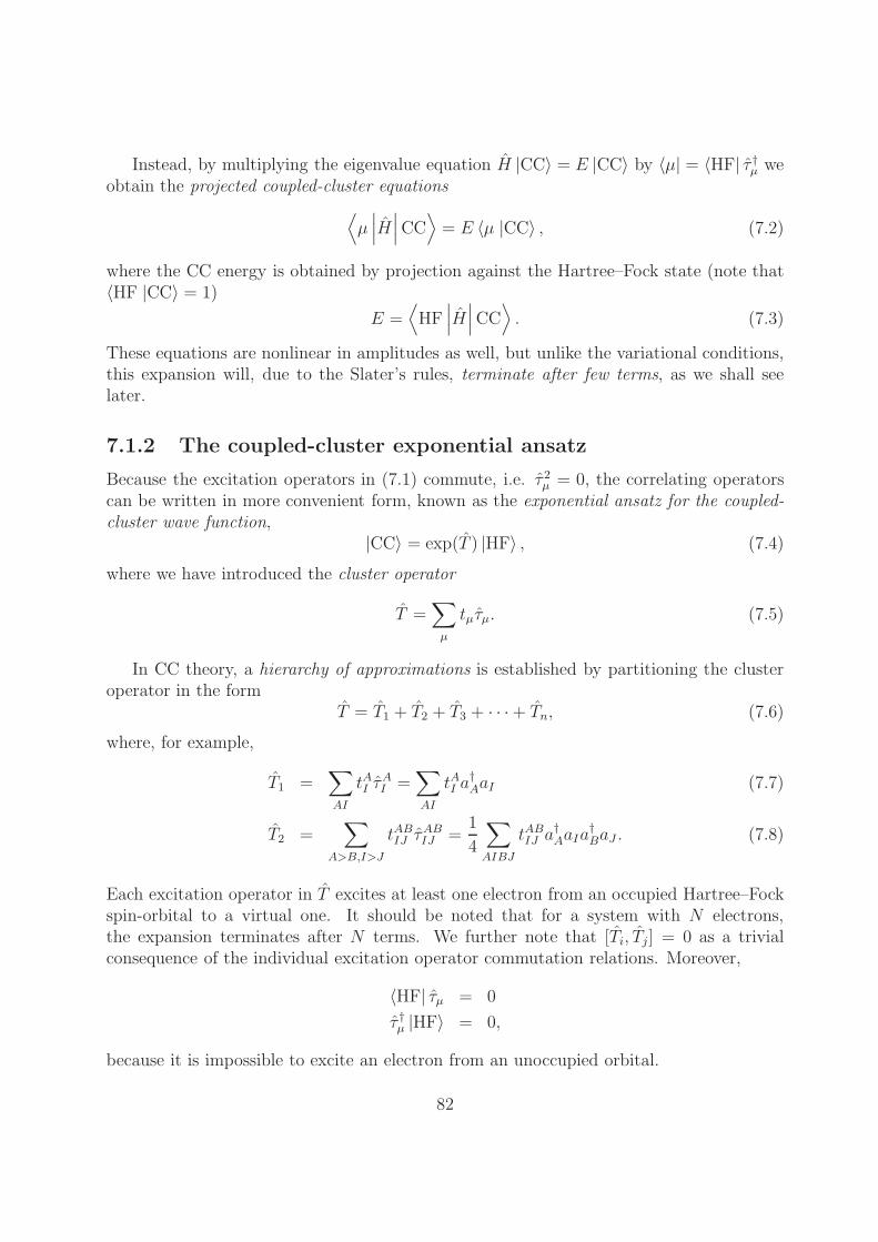
Instead, by multiplying the eigenvalue equation H |CC〉 = E |CC〉 by 〈µ| = 〈HF| τ †µ weobtain the projected coupled-cluster equations

⟨

µ∣∣∣H∣∣∣CC

⟩

= E 〈µ |CC〉 , (7.2)

where the CC energy is obtained by projection against the Hartree–Fock state (note that〈HF |CC〉 = 1)

E =⟨

HF∣∣∣H∣∣∣CC

⟩

. (7.3)

These equations are nonlinear in amplitudes as well, but unlike the variational conditions,this expansion will, due to the Slater’s rules, terminate after few terms, as we shall seelater.

7.1.2 The coupled-cluster exponential ansatz

Because the excitation operators in (7.1) commute, i.e. τ 2µ = 0, the correlating operators

can be written in more convenient form, known as the exponential ansatz for the coupled-cluster wave function,

|CC〉 = exp(T ) |HF〉 , (7.4)

where we have introduced the cluster operator

T =∑

µ

tµτµ. (7.5)

In CC theory, a hierarchy of approximations is established by partitioning the clusteroperator in the form

T = T1 + T2 + T3 + · · ·+ Tn, (7.6)

where, for example,

T1 =∑

AI

tAI τAI =

∑

AI

tAI a†AaI (7.7)

T2 =∑

A>B,I>J

tABIJ τ

ABIJ =

1

4

∑

AIBJ

tABIJ a

†AaIa

†BaJ . (7.8)

Each excitation operator in T excites at least one electron from an occupied Hartree–Fockspin-orbital to a virtual one. It should be noted that for a system with N electrons,the expansion terminates after N terms. We further note that [Ti, Tj] = 0 as a trivialconsequence of the individual excitation operator commutation relations. Moreover,

〈HF| τµ = 0

τ †µ |HF〉 = 0,

because it is impossible to excite an electron from an unoccupied orbital.

82

To compare the CC model with the CI model, we expand the exponential operator andcollect terms to the same order in excitation level:

exp(T ) |HF〉 =N∑

i=0

Ci |HF〉 .

The lowest-order operators Ci are given by

C0 = 1

C1 = T1

C2 = T2 +1

2!T 2

1

C3 = T3 + T1T2 +1

3!T 3

1

C4 = T4 + T3T1 +1

2!T 2

1 T2 +1

4!T 4

1 ,

demonstrating the composition of the excitation processes. The advantages of the clusterparameterization arise in truncated wave functions and are related to the fact that even atthe truncated level, the coupled-cluster state contains contributions from all determinantsin the FCI wave function, with weights obtained from the different excitation processes.

Similarly with the CI theory, a hierarchy of CC models is introduced by truncating thecluster operator at different excitation levels. The simplest successful CC wave functionis the coupled-cluster singles-and-doubles (CCSD) model. In this model, the T2 operatordescribes the electron-pair interactions and T1 carries out the corresponding orbital re-laxations. Its computational cost scales as O(N6). For higher accuracy, the connectedtriple excitations have to be taken into account, which leads to the coupled-cluster singles-doubles-and-triples (CCSDT) model. This model describes already the dynamical correla-tion almost perfectly, but is computationally very demanding, O(N8) and is thus applicableto smallest molecules only. The triples excitations can be estimated in a perturbationalway, giving rise to the CCSD(T) method, which is a good compromise between the com-putational cost (exhibiting an O(N7) scaling) and accuracy. It is often considered to bethe best single-reference treatment of molecular Schrodinger equation that is applicable inpractise.

7.1.3 CI and CC models compared

Let us at this point compare the CI and CC hierarchies. Owing to the disconnectedclusters, CC wave functions truncated at a given excitation level also contain contributionsfrom determinants corresponding to higher-order excitations; whereas CI wave functionstruncated at the same level contain contributions only from determinants up to this level.This is reflected in the convergence towards the FCI limit, which is typical of small systems.For larger systems, CI starts to behave very badly, while the CC description is unaffectedby the number of electrons.

83

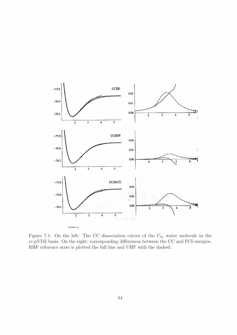
Figure 7.1: On the left: The CC dissociation curves of the C2v water molecule in thecc-pVDZ basis. On the right: corresponding differences between the CC and FCI energies.RHF reference state is plotted the full line and UHF with the dashed.

84

Figure 7.2: The error with respect to FCI of CC and CI wave functions for the watermolecule at the equilibrium geometry in the cc-pVDZ basis.

According to the previous discussion, the projected coupled-cluster equations are writ-ten as

⟨

HF∣∣∣H exp(T )

∣∣∣HF

⟩

= E (7.9)⟨

µ∣∣∣H exp(T )

∣∣∣HF

⟩

= E⟨

µ∣∣∣exp(T )

∣∣∣HF

⟩

. (7.10)

• The excited projection manifold 〈µ| comprises the full set of all determinants up tothe chosen truncation level.

• For the full CC wave function, the number of equations is equal to the numberof determinants and the solution of the projected equations recovers the FCI wavefunction.

• The nonlinear equations (7.9) must be solved iteratively, substituting in every itera-tion the CC energy calculated from (7.10).

It is convenient to rewrite the projected CC equations using the non-Hermitian similarity-

transformed Hamiltonian ˆH = exp(−T )H exp(T ):

⟨

HF∣∣∣exp(−T )H exp(T )

∣∣∣HF

⟩

= E (7.11)⟨

µ∣∣∣exp(−T )H exp(T )

∣∣∣HF

⟩

= 0 (7.12)

The equations (7.10) and (7.12) are completely equivalent (yet the equivalence is nontrivialfor all the truncated CC models!), meaning that they yield same amplitudes and energyupon solution. They are referred to as the unlinked and linked coupled-cluster equations,respectively. Their computational cost is practically the same, but the linked equations

85

have some advantages: Although both yield the same, size-extensive wave function, thelinked equations are size-extensive term by term, that simplifies some perturbational treat-ments; in addition, the CC approach excited states in mind is more fruitful to start fromthe linked equations. The main reason is however the following:

• When the Baker–Campbell–Hausdorff (BCH) expansion

exp(A)B exp(−A) = B + [A,B] +1

2![A, [A,B]] +

1

3![A, [A, [A,B]]] + · · · (7.13)

is applied to the similarity-transformed Hamiltonian, one obtains

exp(−T )H exp(T ) = H+[H, T ]+1

2[[H, T ], T ]+

1

6[[[H, T ], T ], T ]+

1

24[[[[H, T ], T ], T ], T ],

(7.14)the coupled-cluster equations are therefore no higher than quartic in the cluster am-plitudes – for any truncation level or even for the full CC expansion.

• Due to the Brillouin theorem, the one-particle operators contribute only to secondorder. Furthermore, cluster operators higher than the doubles do not contribute tothe CC energy since H is a two-particle operator. As a result, only singles and doublesamplitudes contribute directly to the CC energy – irrespective of the truncation levelof the cluster operator. Of course, the higher-order excitations contribute indirectly,since all amplitudes are coupled by the projected equations.

7.1.4 On coupled-cluster optimization techniques

The elements of the left-hand side of the CC amplitude equation (7.12) constitute thecoupled-cluster vector function Ωµ(t), which can be expanded around the set of amplitudesof the current iteration t(n):

Ω(t(n) + ∆t) = Ω(0)(t(n)) + Ω(1)(t(n)∆t + · · · ,

where Ω(0) is the vector function calculated from the amplitudes t(n) and Ω(1) the CCJacobian

Ω(1)µν =

⟨

µ∣∣∣exp(−T (n))[H, τν ] exp(T (n))

∣∣∣HF

⟩

. (7.15)

Then an iterative scheme is established:

• Solve the set of linear equations

Ω(1)(t(n))∆t(n) = −Ω(0)(t(n)) (7.16)

for ∆t(n)

• Form the improved estimate

t(n+1) = t(n) + ∆t(n) (7.17)

86

• Iterate Equations (7.16) and (7.17) until convergence in the amplitudes.

In more sophisticated implementations, this Newton-method-like approach is replaced bya scheme, where the solution of the linear equations as well as the construction of theJacobian are avoided by the approximation

∆t(n)µ = −ε−1

µ Ω(0)µ (t(n)), (7.18)

where, e.g. εabij = (ǫa + ǫb − ǫi − ǫj). Usually, the convergence is accelerated by the DIIS

method.

7.1.5 The closed-shell CCSD model

We consider now in detail the important special case of CC theory: the closed-shell CCSDmodel. We recall that the singlet CCSD state is generated by |CC〉 = exp(T1 + T2) |HF〉,hence only those terms in Ti that transform as singlet operators should be retained in thecluster operator. It is easy to show that

[

S±, Ti

]

= 0 (7.19)[

Sz, Ti

]

= 0. (7.20)

These impose important constraints on the cluster amplitudes in the spin-orbital basis.Due to these, the singles cluster operator becomes

T1 =∑

ai

tai Eai (7.21)

and the doubles operator

T2 =1

2

∑

aibj

tabijEaiEbj . (7.22)

The cluster amplitudes are symmetric: tabij = tbaji .

The CCSD energy is obtained from Eq. (7.11). By noting that 〈HF| exp(−T ) = 〈HF|,expanding the cluster operators and after some algebra we obtain the form

ECCSD = EHF +1

2

⟨

HF∣∣∣[[H, T1], T1]

∣∣∣HF

⟩

+⟨

HF∣∣∣[H, T2]

∣∣∣HF

⟩

, (7.23)

where the Hartree–Fock energy is given by EHF =⟨

HF∣∣∣H∣∣∣HF

⟩

. By inserting the CCSD

operators to the energy expression and calculating the commutators explicitly we obtain

ECCSD = EHF +1

2

∑

aibj

tai tbj

⟨

HF∣∣∣[[H, Eai], Ebj ]

∣∣∣HF

⟩

+1

2

∑

aibj

tabij

⟨

HF∣∣∣[H, EaiEbj ]

∣∣∣HF

⟩

= EHF +1

2

∑

aibj

(tabij + tai t

bj

) ⟨

HF∣∣∣[[H, Eai], Ebj ]

∣∣∣HF

⟩

= EHF +∑

aibj

(tabij + tai t

bj

)Liajb, (7.24)

87

where we have denoted Lpqrs = 2gpqrs − gpsrq.

7.1.6 The equation-of-motion coupled-cluster method

In CC theory, we arrive at a good description of the ground state. The excited statescould be examined by carrying out separate, independent calculation for each state ofinterest, using in each case some appropriate zero-order reference determinant. However,it is usually difficult or even impossible to determine these adequate reference determinants;it is expensive to carry out individual calculations; and the states obtained in this mannerare not orthogonal, which hinders the identification of the excited states.

Instead, we calculate the excited states in the spirit of CI theory, by a linear expansionin the space spanned by all states of the form

|c〉 =∑

µ

cµτµ |CC〉 = exp(T )∑

µ

cµτµ |HF〉 , (7.25)

where the summation is carried out over all the excitation operators present in the clusteroperator. This expansion is referred to as the equation-of-motion coupled-cluster (EOM-CC) model. The expansion parameters are optimized by the minimization of the energy

E(c, c) =

⟨

c

∣∣∣exp(−T )H exp(T )

∣∣∣ c⟩

〈c |c〉 . (7.26)

The EOM-CC theory can be thought as conventional CI theory with a similarity-transformed Hamiltonian, which carries the information about electron correlation; whilethe configuration expansions carry the information about the excitation structure of theelectronic states.

7.1.7 Orbital-optimized coupled-cluster theory

In the standard CC theory, we use the Hartree–Fock orbitals and then determine a set ofnon-zero single-excitation amplitudes together with higher-excitation amplitudes. Alter-natively, we could use exp(T1) to generate an orbital transformation to a basis in which thesingle-excitation amplitudes vanish. This is the idea behind the orbital-optimized (OCC)theory, in which the orbital-rotation operator exp(−κ) is used instead of exp(T1) (as theygenerate the same state to first order),

|OCC〉 = exp(−κ) exp(TO) |0〉 , (7.27)

where TO = T2 + T3 + · · · + TN . The OCC energy is obtained in the usual manner byprojecting the OCC Schrodinger equation against the reference state

EOCC =⟨

0∣∣∣exp(−TO) exp(κ)H exp(−κ) exp(TO)

∣∣∣ 0⟩

, (7.28)

88

whereas the cluster amplitudes are determined by projection against the manifold |µO〉spanned by TO ⟨

µO

∣∣∣exp(−TO)H exp(−κ) exp(TO)

∣∣∣ 0⟩

= 0. (7.29)

The Brueckner coupled-cluster theory (BCC) is closely related to OCC and differs in somedetails of the solution of orbital rotation parameters. Unlike in standard CC theory, theOCC and BCC orbitals are optimized simultaneously with the optimization of the clusteramplitudes – compare with the MCSCF theory. Surprisingly, the differences between stan-dard and OCC/BCC wave functions are small. Only in the rare cases that are characterizedby the sc. Hartree–Fock singlet instability the OCC/BCC are clearly more successful thanthe standard formulation.

7.2 Perturbation theory

Finally, we consider less rigorous but computationally more appealing improvements of theHartree–Fock description, based on perturbation theory. They are rather successful, whenthe Hartree–Fock wave function is reasonably accurate.

In Møller–Plesset perturbation theory (MPPT) the electronic Hamiltonian is partitionedas

H = f + Φ (7.30)

where f is the Fock operator (5.3) and Φ the fluctuation potential, which is the differencebetween the true two-electron Coulomb potential in H and the effective one-electron po-tential V of the Fock operator, Φ = g − V . The zero-order state is represented by theHartree–Fock state in the canonical representation, that is f |HF〉 =

∑

I ǫI |HF〉, and byapplying the standard machinery of perturbation theory, we obtain to second order in theperturbation

E(0)MP =

⟨

HF∣∣∣f∣∣∣HF

⟩

=∑

I

ǫI (7.31)

E(1)MP =

⟨

HF∣∣∣Φ∣∣∣HF

⟩

(7.32)

E(2)MP = −

∑

A>B,I>J

|gAIBJ − gAJBI |2ǫA + ǫB − ǫI − ǫJ

. (7.33)

Thus, the Hartree–Fock energy is equal to the sum of the zero- and first-order contribu-tions; and by adding the second-order correction, we obtain the second-order Møller–Plessetenergy (MP2)

EMP2 = EHF −∑

A>B,I>J

|gAIBJ − gAJBI |2ǫA + ǫB − ǫI − ǫJ

, (7.34)

which is very popular and successful approach to introducing electron correlation on top ofthe Hartree–Fock wave function; providing surprisingly accurate and size-extensive correc-tion at low computational cost. Higher-order corrections are derived in a similar manner,

89

Figure 7.3: The MPn dissociation curves of the C2v water molecule in the cc-pVDZ basis.Restricted MP2 with full and unrestricted with dashed line.

yielding MP3 and MP4 models, but these become rather expensive and are not as appeal-ing compromise between cost and accuracy as MP2 is. Furthermore, the MPPT series havebeen shown to be inherently divergent.

In the coupled-cluster perturbation theory (CCPT) the Hamiltonian in the CC equa-tions (7.11) and (7.12) is partitioned as in Eq. (7.30). The Fock and the cluster operatorobey the following results:

[

f , T]

=∑

µ

εµtµτµ

[[

f , T]

, T]

= [[[f , T ], T ], T ] = · · · = 0.

Thus we may write the non-Hermitian similarity-transformed Fock operator as

ˆf = f +∑

µ

εµtµτµ, (7.35)

90

and we arrive at the working equations of the CCPT:

E = E0 +⟨

HF∣∣∣ˆΦ∣∣∣HF

⟩

(7.36)

εµtµ = −⟨

µ∣∣∣ˆΦ∣∣∣HF

⟩

. (7.37)

By expanding the cluster operator in the orders of the fluctuation potential we arrive atthe amplitude equations

εµt(n)µ = −

⟨

µ∣∣∣[ ˆΦ](n)

∣∣∣HF

⟩

(7.38)

where [ ˆΦ](n) contains the nth order part of the similarity-transformed fluctuation potential.Then the amplitudes would be determined self-consistently from the projected equationsafter truncating the cluster operator at some excitation level. The CCPT is most oftenused to establish approximations to contributions from some excitations – the most famousis the non-iterative triples, or (T) correction to the CCSD wave function. Also very suc-cessful iterative CCPT schemes have been set up, e.g. the CC2 model approximates theCCSD model with the computational cost O(N5) and CC3 the CCSDT model with thecomputational cost O(N7). The CCPT series provides more systematic improvement tothe wave function than the MPPT.

Both MPPT and CCPT are limited to the ground states of systems dominated by asingle configuration. To overcome this, multiconfigurational perturbation theory has beendeveloped. Most important such theory is CAS perturbation theory (CASPT), where thezero-order state is taken to be a CASSCF wave function. At the moment, it is the onlygenerally applicable method for the ab initio calculation of dynamical correlation effects ofopen- and closed-shell multiconfigurational electronic system.

7.3 Local correlation methods

Traditional correlated electronic wave function methods, which are built upon the de-localized Hartree–Fock molecular orbitals (MO) do not exploit the fact that the elec-tron correlation—i.e., the electron-electron Coulomb cusp—is spatially a rather local phe-nomenon.

In the recent literature, localized correlation methods have been pursued to overcomethe “scaling wall” encountered in the correlated wave function methods. However, despiterecent progress, there is still a need to formulate and implement new approaches thatexploit the locality of the electron correlation problem.

• Approaches based on introducing locality in the correlation treatment using localizedMOs (LMO) appeared already in 1960s and in the context of CC methods in 1980s.

• An alternative approach was presented by Head-Gordon et al., who formulated theCC equations in a general non-orthogonal [e.g., the atomic orbital] basis using ageneral tensor-based formulation. Scuseria and Ayala presented a transformation

91

of the standard MO CC doubles (CCD) equations into the AO basis. Scuseria andAyala argued that the solution of the CC equations in the AO basis scales in principlelinearly with respect to N , but their approach seems so far not to have received anywidespread use.

• A fully operational local CCSD implementation have been presented by Werner et al.This implementation, referred to as the local CCSD (LCCSD) method, is based onlocalizing the occupied space as suggested by Pulay and coworkers, using traditionalMO localization schemes, and using for the virtual space a projected atomic orbital(PAO) basis. LCCSD further relies on a spatial division of the system into domains.Restrictions on the extent to which the interactions between different domains areaccounted for is important for achieving the low-power scaling of LCCSD making theresults deviate from the standard CCSD results.

• The equations of correlated wave function theories may also be derived in a biorthog-onal projected atomic orbital basis, aiming at a black-box formulation that could beapplied to large systems. This formulation also constitutes a good platform to intro-duce efficient approximation schemes to reduce the number of parameters and thusthe computational scaling. The locality of the PAO basis is reflected in the factthat the cluster amplitudes, the integrals as well as the correlation energy contri-butions decay exponentially with respect to the distance between the centers of theparticipating PAOs.

92

7.4 Further reading

• T. Helgaker, P. Jørgensen, J. Olsen, Molecular Electronic-Structure Theory (Wiley2002), pp. 648–816.

• T. J. Lee and G. E. Scuseria, Achieving chemical accuracy with coupled-cluster theory,in S. R. Langhoff (ed), Quantum-Mechanical Electronic Structure Calculations withChemical Accuracy (Kluwer 1995).

• O. Christiansen, Coupled cluster theory with emphasis on selected new developments,Theor. Chim. Acta 116, 106 (2006).

7.5 Exercises for Chapter 7

1. Evaluate the commutator [H, Eai] and the expression for this commutator applied tothe Hartree–Fock state [H, Eai] |HF〉.

2. Verify the overlap between the doubly excited states:

⟨abij

∣∣∣∣

cdkl

⟩

= 4δacδbdδikδjl + 4δadδbcδilδjk − 2δacδbdδilδjk − 24δadδbcδikδjl

= 2P abij (2δaibj,ckdl − δajbi,ckdl).

The operator P carries out the permutation P abij A

abij = Aab

ij + Abaji .

3. ⋆ Verify the following commutation relations:

[[

H, Eai

]

, Ebj

]

= −P abij hibEaj − P ab

ij

∑

pq

(gpbiqepjaq + gpqjaepqbi)

+∑

pq

(gpbqaepjqi + gjpiqebpaq)

[[[

H, Eai

]

, Ebj

]

, Eck

]

= P abcijk

∑

p

(gkbipepbic + gpbicepjak) ,

and the expressions for these commutators applied to the Hartree–Fock state:

[[

H, Eai

]

, Ebj

]

|HF〉 = 2Liajb |HF〉

−P abij

(

IFibEaj +∑

k

LikjbEak −∑

c

LcajbEci

)

|HF〉

+

(∑

bjc

gbjcaEbjEci −∑

bjk

gbjikEbjEak

)

|HF〉

93

[[[

H, Eai

]

, Ebj

]

, Eck

]

|HF〉 = −P abcijk LjbicEak |HF〉

+P abcijk

(∑

l

giljcEalEbk −∑

d

gidbcEajEdk

)

|HF〉 .

In the above, we have introduced the notation Lpqrs = 2gpqrs − gpsrq as well as usedthe three-index permutation operator,

P abcijk A

abcijk = Aabc

ijk + Aacbikj + Abac

jik + Abcajki + Acba

kji.

4. ⋆ Consider, once again, the H2 molecule in a minimal basis.

(a) Show that the cluster operator becomes

T = T2 =1

2tuugg EugEug

and that the biorthogonal basis can be expressed as

⟨uugg

∣∣∣∣= 〈vac| auβauα.

(b) Show that the unlinked coupled-cluster equations can be expressed as

⟨

HF∣∣∣H(1 + T2)

∣∣∣HF

⟩

= E⟨uugg

∣∣∣H(1 + T2)

∣∣∣HF

⟩

= E

⟨uugg

∣∣∣T2

∣∣∣HF

⟩

.

(c) Show that the linked coupled-cluster equations are

⟨

HF∣∣∣H(1 + T2)

∣∣∣HF

⟩

= E⟨uugg

∣∣∣(1 − T2)H(1 + T2)

∣∣∣HF

⟩

= 0.

(d) Show, that the linked and unlinked coupled-cluster equations are equivalent.

5. ⋆ Construct expressions for the CCSD vector functions

Ωai =

⟨ai

∣∣∣exp(−T2)H exp(T2)

∣∣∣HF

⟩

Ωaibj =

⟨abij

∣∣∣exp(−T2)H exp(T2)

∣∣∣HF

⟩

94

6. ⋆ The basic idea behind the quantum-mechanical perturbation theory (known as theRayleigh–Schrodinger perturbation theory, RSPT) is to partition the Hamiltonianinto two parts, H = H0 + U , where H0 is some zero-order Hamiltonian and U theperturbation H−H0. The orthonormal eigensolutions to the zero-order Hamiltonian,∣∣Ψ(0)

⟩with the corresponding energy E(0) are then used to expand the eigenfunction

|Ψ〉 of the exact Hamiltonian.

(a) Show, that

(H0 − E(0))∣∣Ψ(n)

⟩= −U

∣∣Ψ(n−1)

⟩+ +

n∑

k=1

E(k)∣∣Ψ(n−k)

⟩

and that all corrections to the zero-order energy are obtained as

E(n) =⟨

Ψ(0)∣∣∣U∣∣∣Ψ(n−1)

⟩

.

(b) Write out explicitly three lowest-order corrections to the energy and to the wavefunction.

7. ⋆ Consider the wave function correct to nth order in RSPT:

|Ψn〉 =

n∑

i=0

∣∣Ψ(i)

⟩.

Show that the energy calculated as the expectation value

E =

⟨

Ψn

∣∣∣H∣∣∣Ψn

⟩

〈Ψn |Ψn〉is correct to order 2n+ 1. This result is known as the Wigner’s rule. In addition, asa special case, consider the wave function correct to first order, |Ψ1〉 =

∣∣Ψ(0)

⟩+∣∣Ψ(1)

⟩

and show that the expectation value may then be expressed in terms of the RSPTcorrections as ⟨

Ψ1

∣∣∣H∣∣∣Ψ1

⟩

〈Ψ1 |Ψ1〉= E(0) + E(1) +

E(2) + E(3)

1 + 〈Ψ(1) |Ψ(1)〉 .

8. ⋆ Here we generalize the RSPT formalism to the expansion of the perturbed states∣∣Ψ(n)

⟩=∑

i

C(n)i |i〉

in a nonorthogonal basis, whose overlap elements differ from the Kronecker delta:〈i |j〉 6= δij .

(a) Show that the zero-order equations and the condition for the intermediate nor-malization become

H0C(0) = E(0)SC(0)

(C(0))TSC(0) = 0.

95

96

Chapter 8

Performance of the

electronic-structure models

Having now considered the most important approximations to the molecular electronicwave function we will now address their performance in terms of a few numerical examples.It should be remembered that none of these models (besides FCI, which is inapplicable formost cases) is an all-around-good one: good performance in some problem and/or in somesystem does not guarantee good performance in another situation. In addition, rehearsethe graph concerning the approximations to the one- and N -electron spaces.

8.1 Molecular equilibrium geometries

One of the most common applications of molecular electronic-structure calculations isthe determination of the molecular equilibrium structures. Good geometries are also offundamental importance in study of molecular properties.

We consider the mean errors and standard deviations of calculated bond distances andbond angles as compared to experimental results using a hierarchy of N -electron modelsand a hierarchy of Gaussian basis sets. The error is given by ∆ = P calc

i − P expi , and the

mean error and standard deviation by

∆ =1

n

n∑

i=1

∆i (8.1)

∆std =

√√√√

1

n− 1

n∑

i=1

(∆i − ∆)2. (8.2)

They can be conveniently represented graphically in terms of the normal distribution

ρ(P ) = Nc exp

[

−1

2

(P − ∆

∆std

)2]

. (8.3)

97

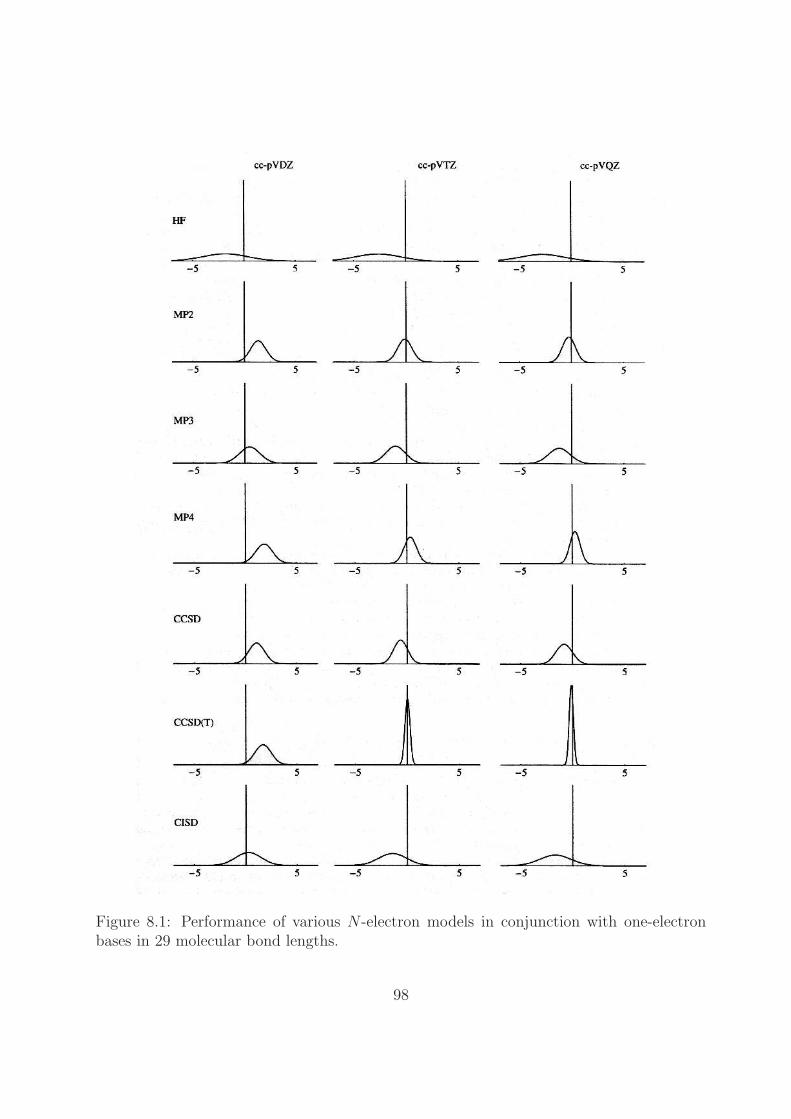
Figure 8.1: Performance of various N -electron models in conjunction with one-electronbases in 29 molecular bond lengths.

98

The calculations were carried out for sets of small molecules containing main-group ele-ments. 29 bond distances and 10 bond angles were calculated, and the results are presentedin Figures 8.1 and 8.2.

Observations:

• The Hartree–Fock model is suitable for only preliminary calculations.

• The CCSD(T) model is capable of providing structures – both bond distances andangles – of high quality.

• The MP2 model is less accurate but more generally applicable as it is considerably lessexpensive. Higher-order MPPT is significantly less accurate but hideously expensive,i.e., useless.

• The performance of the CCSD model is disappointing. It however performs morerobust than MP2 in some selected cases with complicated electronic structure.

• The CISD model is also rather useless, showing no improvement when the basis setis increased.

• The basis-set requirements are different for different models. Whereas there is nomuch use to use QZ-level basis sets with the Hartree–Fock model (as the resultsare not improved), the correlated models require at least a TZ-level basis set, butpreferably the cc-pVQZ basis.

The results suggest the following recipe for the determination of molecular structures:obtain an initial structure with HF using a DZ-level basis and improve it by using MP2and a TZ basis. If ever possible, calculate the final geometry in the cc-pVQZ basis usingthe CCSD(T) model.

8.2 Molecular dipole moments

The comparison between the experimental and calculated molecular dipole moments isdifficult, as the experiments are measuring the dipole moment in the vibrational groundstate µ0, whereas the calculations are carried out for the equilibrium dipole moment µe,and thus we would have to carry out a vibrational averaging in order to speak of the samequantity. However, there are a few experimental values for µe, and we shall compare theperformance of our standard models with those. Note, that due to the outer-valence originof this property, we have to augment our basis sets with extra diffuse primitive Gaussians;hence we are using the aug-cc-pVXZ basis sets. The geometries are optimized using thesame wave function as for the calculation of the dipole moment.

We observe from Table 8.1, that the quality of the calculation is more dependent onthe correlation treatment than the cardinal number of the basis set; yet it is necessary toaugment the basis set. The further augmentation (d-aug-cc-pVXZ basis sets) of the basisset does not affect the calculated dipole moments significantly.

99

Figure 8.2: Performance of various N -electron models in conjunction with one-electronbases in 10 molecular bond angles.

100

Figure 8.3: Changes in bond lengths calculated from ∆ of the cc-pVQZ basis.

Exp. HF MP2 CCSD CCSD(T)QZ QZ QZ DZ TZ QZ

NH3 1.561(5) 1.544 1.517 1.530 1.541 1.513 1.521HF 1.803(2) 1.884 1.811 1.813 1.799 1.797 1.800H2O 1.8473(10) 1.936 1.864 1.870 1.859 1.845 1.853

Table 8.1: Calculated dipole moments.

101

Figure 8.4: Reaction enthalpies.

8.3 Reaction enthalpies

Next, we study the reaction enthalpies of 13 chemical reactions among closed-shell molecules.The calculations are carried out in the HF–MP2–CCSD–CCSD(T) hierarchy, using thecorrelation-consistent basis set hierarchy supplemented with steep functions to providecore-polarization, which – somewhat surprisingly – must be included in the high-precisioncalculation of reaction enthalpies. The results are illustrated in Figure 8.4.

8.4 Notes on total electronic energies

For the total molecular energy, i.e., E in the molecular Schrodinger equation, there is noexperimental counterpart. and we examine it in order to establish a feeling on the sever-ity of the approximations involved in the calculation. We should recall that there were athird class of approximations in addition to the truncation of one- and N -electron spaces:approximations in the molecular Hamiltonian H. To investigate the validity of the use ofthe non-relativistic Hamiltonian, we include the leading-order one-electron relativistic cor-rections that include the spin-orbit interaction (SO), mass-velocity (MV), and the Darwin(Dar) corrections. The leading-order two-electron contributions, such as the two-electronDarwin contribution and the spin-spin contact interaction, are smaller by at least one orderof magnitude. The MV and Dar corrections are always of opposite sign. The calculationis carried out using the CCSDT model for the water molecule in the cc-pCVXZ bases ata CCSD(T)/cc-pCVQZ geometry.

Observations:

102

Total energy [Eh] Energy corrections [mEh]CCSDT HF HF→SD SD→(T) (T)→T SO MV Dar

DZ -76.24121 -76.02680 -211.21 -3.04 -0.16TZ -76.33228 -76.05716 -267.40 -7.65 -0.08QZ -76.35981 -76.06482 -285.98 -8.99 -0.01 0.00 -255.87 203.695Z -76.36899 -76.06708 -292.44 -9.52 0.04

Table 8.2: Decomposition of the CCSDT energy of water.

• It is remarkable how a tiny, less than one per cent fraction of the total energy, playssuch an important role in the determination of molecular properties.

• The leading-order relativistic correction, -52.18 mEh, is larger than the triples con-tribution already in water, and gets far more pronounced in systems with heavierelements present!

• (T) is a very good approximation to full triples.

103