pelagic fisheries research program - soest.hawaii.edu file2/17 2 3 l2 3m 33 22 ? i ˚ p light based...
TRANSCRIPT

1/17 P�i?22333ML232
Pelagic Fisheries Research Programhttp://www.soest.hawaii.edu/PFRP/
A mosaic of models for light-based geolocation:
How to choose, what to be careful about, and
future directions
Anders Nielsen & John Sibert

2/17 P�i?22333ML232
Light based geolocation
� We got:
– Light, depth, and temperature
– Measured for instance every minute
– From archival tags the entire record can be retrieved
– From satellite transmitting tags only a summary
� We want:
– A track of geographic positions (geolocations)
– Some idea about the uncertainties
– Perhaps some quantitative movement parameters
� Problems:
– Indirect measurements: Light → solar altitude → geolocation
– High and correlated uncertainties from changing weather and incomplete depthcorrections

3/17 P�i?22333ML232
This talk
� Will talk about:
– Raw geolocations
– Kftrack
– Kfsst/ukfsst
– Trackit (with and without SST)
� Will not talk about:
– Satellite methods
– Tidal location models
– Sunrise/sunset times models
– SST matching algorithms
– EASy-FishTracker
– ...
4/17 P�i?22333ML232
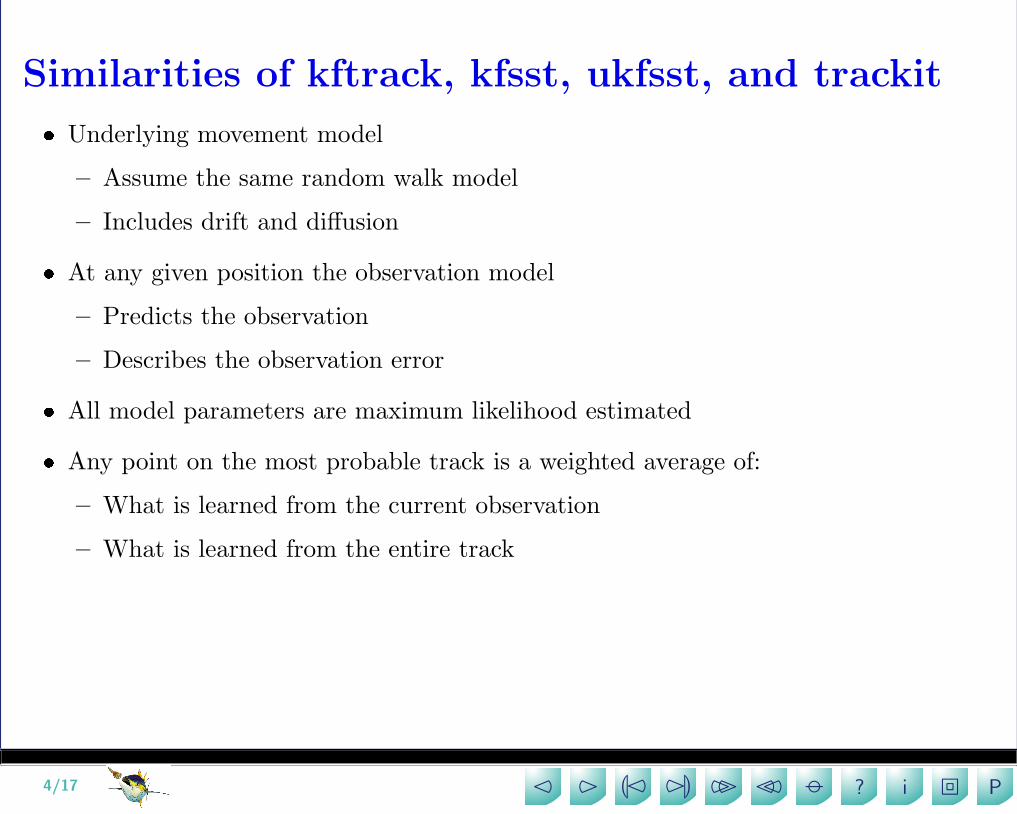
Similarities of kftrack, kfsst, ukfsst, and trackit
� Underlying movement model
– Assume the same random walk model
– Includes drift and diffusion
� At any given position the observation model
– Predicts the observation
– Describes the observation error
� All model parameters are maximum likelihood estimated
� Any point on the most probable track is a weighted average of:
– What is learned from the current observation
– What is learned from the entire track

5/17 P�i?22333ML232
The differences are
� What they take as data
– Raw geolocations (lon,lat) used by kftrack
– Raw geolocations and SST (lon,lat,SST) used by kfsst and ukfsst
– Light readings and SST used by trackit
� Technical details in handling non-linearities
– Extended Kalman filter used by kftrack and kfsst
– Unscented Kalman filter used by ukfsst and trackit
(lon,lat) SST Light EKF UKF
kftrack X X
kfsst X X X
ukfsst X X X
trackit X X X
If possible, running more than one can often be very instructive ...

6/17 P�i?22333ML232
'
&
$
%?
Raw geolocation
?(lon,lat)
'
&
$
%?
Raw geolocation
?(lon,lat)
'
&
$
%?
Raw geolocation
?(lon,lat)
� Algorithms (partly) proprietary, but in essence:
– Associate a certain light level crossing with a solar angle (problematic)
– Calculate position from two of those
� These raw geolocations are often imprecise and biased
� Especially latitude around equinox

7/17 P�i?22333ML232
'
&
$
%?
Raw geolocation
?(lon,lat)
'
&
$
%?
Raw geolocation
?(lon,lat)
'
&
$
%?
Raw geolocation
?(lon,lat)
Kftrack
PPPPPPPPPPPq
AAAAU
����������)
day month year lon lat
21 1 1999 201.750 18.65
22 1 1999 204.520 20.00
23 1 1999 206.086 22.00
24 1 1999 204.399 23.50
.
.
.
library(kftrack)
track<-read.table(’datafile.dat’, header=TRUE)
fit<-kftrack(track)
plot(fit, map=TRUE, ci=TRUE)

8/17 P�i?22333ML232
'
&
$
%?
Raw geolocation
?(lon,lat,SST)
'
&
$
%?
Raw geolocation
?(lon,lat,SST)
'
&
$
%?
Raw geolocation
?(lon,lat,SST)
Kfsst/ukfsst
HHHHHHHHj
AAAAU
��������
day month year lon lat sst
11 4 2001 201.722 18.875 24.73
16 4 2001 201.190 24.150 24.37
18 4 2001 202.950 12.890 24.73
22 4 2001 199.110 28.790 24.37
.
.
.
library(kfsst) or library(ukfsst)
track<-read.table(’datafile.dat’, header=TRUE)
sst.path<-get.sst.from.server(track)
sst.file<-write.sst.field(sst.path) delete line in ukfsst
fit<-kfsst(track)
plot(fit, map=TRUE, ci=TRUE)

9/17 P�i?22333ML232
'
&
$
%
'
&
$
%
'
&
$
%Trackit
PPPPPPPPPPPq
AAAAU
����������)
year month day hour min sec depth light temp
2002 9 11 15 35 53 15.5 69 21.1
2002 9 11 15 36 53 15.0 75 21.1
2002 9 11 15 37 53 16.0 85 21.3
.
.
.
year month day hour min sec sst
2002 9 15 3 0 0 22.4
2002 9 17 2 0 0 23.1
2002 9 21 5 0 0 22.9
.
.
.
library(trackit)
track<-read.table(’datafile.dat’, header=TRUE)
sst<-read.table(’sstdatafile.dat’, header=TRUE)
sst.path<-get.sst.from.server(track,150,250,0,40)
prep.track<-prepit(track, sst=sst,
fix.first=c(198.55,22.85,2002,9,10,0,0,0),
fix.last=c(200.13,21.95,2003,5,21,0,0,0))
fit<-trackit(prep.track)
plot(fit)
fitmap(fit)

10/17 P�i?22333ML232
Be careful about trusting raw geolocationsLo
ngitu
de
200
201
202
203
204
15 35 55 75
Days at liberty
●●
●●●●
●●●
●●
●
●●
●
●●●●●●●
●●●
●●●●●●
●●●●
●●●●●
●●
●●●●●●
●●●
●
●●
●
●
●
●●
●●●●
●●
●●●●●●●●●●
●●●
●●●
●
●
●
●
●
●●
●●●
●●●●●
●●
●●●
●●
●●
●●●
● ●●●●●●
●
●
●
●
●
●
Date
Latit
ude
16
17
18
19
20
21
22
23Aug2003 12Sep2003 2Oct2003 22Oct2003
●
●●●
●●
●●●
●●●●●●
●●●●●●●●●●●●●● ●●●●●●●●●●●●●●●●●●●●●●●
●●●●●●●●●●
●●●●●●
●●●●●●●●●●
●●●●●●●●
●●●●●●●●●●●●●●●●● ●●●●●●
●●
●●●●●●●●●
●
●
●
●●
●●
●
●
●
●●●
●
●●●
●
●
●
●
●●
●
●
●
●
●
●●
●●●●●
●
●●●
●
●
●
●●
●
●
●
●
●
●
●
●
●●●
●
●
●
●
●
●
●
●●
●
●
●
●
●
●
datdate
lon
●●●●●●
●●●●●●
●●
●●●●●●●●●●●
●●●●●●●●●●
●●●●●●●
●●●●●●
●●●●
●●●●●●●●●●●●●
●●●●●●●●●●●●●
●●●●●
●
●
●
●●●●●
●●●●●
●●●●●
●●●●
●●●● ●●●●●●
●
●●●
●
●
15 35 55 75
Days at liberty
200
201
202
203
204
Long
itude
●
●
●●●
●
●
●
●
●
●●
● ●
●
●●●
●
●
●●●
●
●
●
●●●●●●●
●
●
●●●●●●
●●●
●●●●
●●
●●
●●
●●●
●
●
●●
●●●●
●●
●
datdate[i]la
t[i]
●●●●●●●●●●●●●●●●●●●●●●●●● ●●●●●●●●●●●●●●●●●●●●●●●●●●●●●●●●●●●●●●●●●●●●●●●●●●●●●●●●●●●●● ●●●●●●●●●●●●●●●●● ●●●●●● ●●●●●●●●●●● ●
−10
0
10
20
30
40
50
60
Latit
ude
●
●
●
● ●
●●
●
●
●
●●
●●
●
●
●●●
●●●
●●●● ●●●
●●
●
●●
● ●
Date
sst[i
]
●●●●●●●●●●●
●●
●●●●●●●●●●
●●●●●●
●●●●●●●●●●●
●●●●●●●●●●●●
●●●●●●
●●●●●
●●●●●●●●●●●●
●●●●●●●●●●●
●●●●●●●●
●●●●●●●●●
●●●●●● ●●●●●●●●●●●●
23Aug2003 2Oct2003
25.0
25.5
26.0
26.5
27.0
27.5
28.0
SST
HHY SST available

11/17 P�i?22333ML232
Be careful about trusting raw geolocations - 2
205
210
215
220
Long
itude
(E)
16 36 56 76 96
Days at liberty
●●●●
●
●●●●●●●●●●●●
●●●
●
●●●●●●
●●●●●●●●
●
●●●
●
●
●
●●●●●
●●●
●●●●●
●●●●●●
●●●
●●●
●●●
●●
●
●●●●●
●●●●●●●
●●●●●●●●●●●
●●●●●●●●●
●●●
●●●●●●●●●●●●●●●●●●●●
●●●●●●●
●●●●●●●●●●
●●●●●
●●●
●
A
10
15
20
Latit
ude
14Jul2003 3Aug2003 23Aug2003 12Sep2003 2Oct2003
Date
●
●●●●●●●●●
●●●●●●●●●●
●●●●●
●● ●●●●●●●●●●●
●●●● ●●●●●
●●●●●●●●●
●●●●●●●● ●●●●●●●● ●●●●●
●
●●●●●●●
●●●●●●●●●●●●●●●●●●●●●
●●
●●●●●●●
●●●
●●●●●
●●●●●
●●●●●
●●●●●●●●●
●●●●●●●●
●●●
●
B
●●
●
●●●●●
●●
●●●
●
●●
●
●
●
●
●
●
●
●
●●●
●
●
●●
●
●●●
●
●●●●●●●●
●
●
●
●
●
●
●●●●●●●●●●
●●●●●●●●●●●
●●●
●
datdate
lon
C
●●●●●
●●●●●●●●●●●●●●●
●●●●
●●●●●●●●●●●
●●●●
●●●
●●●●●●●
●●●●●●
●●●●●●
●●●
●●●●●
●●●
●
●●●●●
●●●●●●●●●●●●●●●●●●●●●●●
●●●●●●●
●●●●●●●●●●●●●●●●●●●●●●●●●●●●●●●●●●
●●●●●●●●●●●
●
16 36 56 76 96
Days at liberty
205
210
215
220
Long
itude
●
●● ●●●
●
●
●
●
●
●●●●
●
●
●
●
●
●
●
●
●
●
●
●
●
●
●
●
●
●
●
●
●●●●
●
●●
●
●●●●●
●
●●●●●●
●
●
●
●●
●●
●
datdate[i]la
t[i]
D
●●●●●●●●●●●●●●●●●●●●●●●●●●●●●●●●●●●●●●●●●●●●●●●●●●●●●●●●●●●●●●●●●●●●●●●●●●●●●●●●●●●●●●●●●●●●●●●●●●●●●●●●●●●●●●●●●●●●●●●●●●●●●●●●●●●●●●●●●●●●●●●●●●●●●●●●●●
−10
0
10
20
30
40
50
Latit
ude
●
●
●●●●
●
●
● ●●
●●●
●
●●
●
●
●
●
●
●●
●
●
sst[i
]
Date
E
●●●●●●●●
●●●●●●●●●●●●
●●●●●●●●
●●●●●●●●●●●●●●
●●●●●
●●●
●●●●●●●●●●●
●●●
●●●●●●●●●●●●
●●
●●●
●●●●
●●●●●●●●●●
●●●●●●●●●●●
●●●●●●●
●●
●●●
●●●●
●
●
●●●●●●●●●
●●●●●●●●●
●●●●●●●●●
●●●
14Jul2003 23Aug2003 2Oct2003
25
26
27
28
SST

12/17 P�i?22333ML232
Be careful about convergence
#R-KFtrack fit
#Mon Nov 12 16:22:14 2007
#Number of observations: 76
#Negative log likelihood: 322.056
#The convergence criteria was met
� Convergence should be obtained
� Ways to help the optimizer if a track is problematic
– Simplify model (especially for short tracks)(e.g. fit<-kftrack(track, bx.a=FALSE, by.a=FALSE))
– Supply better initial values(e.g. fit<-kftrack(track, D.i=500))
– Remove extreme outliers(e.g. track<-track[abs(track$lat)<90,])
– A combination
– Also check data

13/17 P�i?22333ML232
Be careful about selecting satellite SST data
� In open ocean coarse resolution is fine
� Near the coast a fine resolution is needed
� In areas with frequent cloud cover consider the blended source
� See the options in the documentation?get.sst.from.server
?get.blended.sst
Remember to report back
� Like to hear when it is working
� Need to hear when it is not

14/17 P�i?22333ML232
Future directions
� Grid based methods interesting
– allows other distributions than Gaussian
– allows strong non-linearities (land areas)
– very computational demanding
� Numerous tracks in one model
– The right thing to do if some (or all) parameters are common
– More confidence in estimated parameters
– Possible to allow more flexible movement patterns
� Conventional tracks and archival tags in one model
– First step in using all tagging data in fish stock assessment models
� All packages can be downloaded from:
http://www.soest.hawaii.edu/tag-data/software/
Thank you for listening!

15/17 P�i?22333ML232
Combining individual and population based models
An appealing idea
– The parameters are the same (drift and diffusion)
– All tagged fish from the same population should be equal representatives, no matterwhat type of tag
– Might get better individual tracks when parameter estimates get better
– How much more is learned from an (expensive) archival tag
Simulation study
– 100 data sets are simulated each with 5100 simulated individuals
– 5000 with conventional tags 100 with archival tags (randomly assigned)
– Realistic effort pattern, fishing mortality, and natural mortality are applied
Parameter estimation
– A–D–R model is used for the conventional tags
– The Kalman filter likelihood was extended to include survival and recapture prob-abilities, and the individuals that were not recaptured

16/17 P�i?22333ML232
Results
u
−0.02 0.02 0.06
020
4060
8010
012
014
0
v
−0.02 0.010
2040
6080
100
120
D
0.40 0.50 0.60
02
46
810
12
Q
0.4 0.6
05
1015
2025
30
σ2
−0.02 0.02 0.06
05
1015
2025
−0.02 0.01
05
1015
2025
3035
0.40 0.50 0.60
02
46
810
12
0.4 0.60
12
34
597 100 103
0.00
0.05
0.10
0.15
0.20
0.25
0.30
Hist
ogra
m o
f 100
est
imat
ions
from
100
arch
ival t
ags
5000
con
vent
iona
l tag
s

17/17 P�i?22333ML232
Parameter True Conventional tags Archival tags All tagsname value bias std. dev. bias std. dev. bias std. dev.
u 0.02 -0.00143 0.00259 -0.00364 0.01467 -0.00188 0.00182v 0.00 -0.00232 0.00302 0.00059 0.01150 -0.00134 0.00299D 0.50 -0.02078 0.02403 -0.00244 0.03733 -0.01695 0.01640Q 0.50 -0.00228 0.01221 0.02835 0.08274 -0.00011 0.01164σ2 100.00 -0.13608 1.52063 0.09419 1.34204
– Best results from combined model
– In this setting we get almost the same amount of information about drift (u, v)′ fromone conventional tag as from one archival tag. This will likely change in a morecomplex setting.
– Archival tags provide more information per tag about diffusion D than conventionaltags