peninsula technikon
TRANSCRIPT

PENINSULA TECHNIKON
Department of Electrical Engineering
Faculty of Engineering
AN INVESTIGATION AND DESIGN OF AN INFRAREDRADIATION HEAT PROFILE CONTROLLER
by
Marco Leroy Adonis
Submitted in fulfiIlment of the requirement for
Masters degree of Technology (MTech): Electrical engineering
Under the supervision of
Mohammed Tariq Ekeramodien Khan
DECEMBER 2002

DECLARATION
I, Marco Leroy Adonis, hereby declare that the dissertation presented here is my own
work and the opinions contained herein are my own and do not necessarily reflect those
of the Technikon. All references used have been accurately reported.
Name: Marco Leroy Adonis
Signature: ~--S
Date: December 2002

Acknowledgements
A work of this nature requires the help and support of many people. Though many had a
part in helping me in several ways, some do deserve special mention.
I would like to thank my supervisor, Mr. Mohammed Tariq Ekeramodien Khan, for his
guidance and assistance throughout the time of my research and whose leadership and
direction steered the course of this research to its completion. Mr. P. Mostert also
deserves my thanks and gratitude, he offered the impetus at the conception of this work
and continued throughout to provide meaningful insight. Special mention must be made
of Prof. R. Tzoneva whose expert knowledge of control theory and willingness to help
is greatly appreciated. To the Electrical Department of Peninsula Technikon, thank you
for availing me the facilities in which to continue my research. My gratitude also
extends to my sponsors, the National Research Foundation (NRF), whose financial
assistance provided me a platform to conduct this research, which proved "both
interesting and rewarding.
Then to my family whose support and understanding during this research helped me
focus my efforts and bring it to conclusion. To my fellow research colleagues and
friends, thank you for your motivation and inspiration it proved invaluable.

AN INVESTIGATION AND DESIGN OF AN INFRARED
RADIATION HEAT PROFILE CONTROLLER
by
Marco Leroy Adonis
Abstract
This research outlines the development and design of an infrared radiation heating
profile controller. The study includes both the theoretical aspects of the design process
as well as giving an overview of the practical facets involved. The controller was
subjected to comparative testing with a proportional control model, in order to observe
its performance and validate its effectiveness.
A need exists for these types of controllers and proved to be the motivation to embark
on this investigation. Controllers of this nature that are commercially available either
lacks the functionality of this unit or are too expensive to implement for research
purposes. This unit was designed with cost effectiveness in mind but still meet the
standards required of an industrial style controller. To this end the construction was
completed using low cost and affordable electronic components. Heating profiles are
necessary and useful tools for the proper processing of a host of materials. The
controller developed in this research is able to within a fair degree of accuracy track a
heating profile. The results confirm that this programmable control model to be a
benefit and a valuable tool in temperature regulation. This means that intensive studies
into the effects of infrared radiation on materials are now feasible. Research of this
nature could possibly expand the application of infrared as a heating mechanism.
Although tests were conducted on this controller, they are not meant to serve as an
exhaustive analysis. The conclusions of these examinations do reveal the benefit of such
a controller. More rigorous investigation is suggested as a subject for further study.
11

TABLE OF CONTENTS
TitleDeclarationAcknowledgementsAbstractTable of contentsList of FiguresList of TablesNomenclature
1. INTRODUCTION
1.1 Modes of heat transfer
1.2 Purpose ofthis research
1.3 Typical applications of infrared heating
1.3.1 Drying applications1.4 Concerns addressed by infrared technology
1.4.1 Material damage1.4.2 Cost effectiveness1.4.4 Increased productivity1.4.5 Environmental impact1.4.6 Energy efficiency1.4.7 Time and space savings1.4.8 On-going research1.5 Aim and outline of dissertation
2. BRIEF THEORY OF INFRARED RADIATION
2. I The nature of thermal radiation
2.2 Basic laws and definitions
2.3 Geometric considerations
2.3.1 View factor algebra2.3.1.1 The reciprocity rule2.3.1.2 The summation rule2.3.l.3 The superposition rule2.4 Radiation heat transfer between black surfaces
2.5 Radiation heat transfer between diffuse, gray surfaces in an enclosure.
2.5.1 Net radiation heat transfer at a surface2.5.2 Net radiation heat transfer between surfaces2.6 Methods of solving radiation problems
2.7 Radiation heat transfer in two-surface enclosures
2.8 Radiation heat transfer in three-surface enclosures
III
iiiiiiviixx
1
3
4
55
779999
1010
11
11
13
21
2323242426
26
282829
34
35

2.9 Radiation shields
2.10 Participating Media
2.10.1 Gaseous Emission and Absorption
3. CONTROLLER DESIGN
3.1 Mathematical modeling and experiments
3.1.1 Overview of infrared drying studies3.1.2 Mathematical models of electric IR heaters3.2 Overview of process control aspects
3.2.1 Mathematical description of a control system3.2.2 PID control of the plant3.3 Controller Design
3.3.1 Identification of the infrared oven (heater)3.3.2 Experimental Results for step response of the plant3.3.3 Design ofa continuous controller followed by discretisation
4. PRACTICAL DEVELOPMENT OF THE ill CONTROLLER
4.1 Hardware set-up
4.1.1. The Microcontroller4.1.2 The Power Controller4.1.2.1 AC Power control aspects
- 4.1.2.2 The Triac4.1.2.3 The Triac Power Controller4.1.2.4 The software algorithm4.1.2.5 Evaluation of the triac power control circuit4.1.3 The Insulated Gate BipolarTransistor Power Controller4.1.3.1 The circuit operation4.1.3.2 Evaluation of the low cost IGBT power controller4.1.4 Solid-state switch with PWM cycle control4.1.4.1 Evaluation of the SSS power controller4.2 Infrared Radiation Heater
4.3 Temperature Sensor
4.3.1 Installation considerations4.4 Data Acquisition
4.4.1 National Instruments DAQPad-12004.4.2 80C515 Analog-to-Digital converter
5. Al-"ALYSIS OF RESULTS
5.1 Control system and controller integration
5.2 Comparative testing of the PID controller
IV
38
40
4\
43
43
434546
464852
525356
65
65
6666676772737678~
8285868991
92
9496
9697
98
98
99

5.2.1 Comparative tests at a sampling period of I second 1025.2.2 Comparative tests at a sampling period of lOOms 1055.3 Infrared temperature sensor 108
5.4 Analog-to-digital converter (ADC) 109
5.5 Overview of Analysis 110
6. CONCLUSION AND RECOMMENDATIONS 111
6.1 Problems solved in the dissertation III
6.1.1 Experimentally determine the mathematical model of an IR heater. I 126.1.2 Investigate a hardware platform for the power control of an IR heater. 112
6.1.3 Investigate the various types of temperature control models available. I 136.2 Applications of the results 113
6.3 Recommendations for further study I 13
6.4 Publications in connection with dissertation 114
7. REFERENCES 116
APPENDIX 1 120
APPENDIX 2 122
APPENDIX 3 129
APPENDIX 4 134
APPENDIX 5 139
v

List of Figures
Figure 1.1 Absorbtion spectra of different materials 6
Figure 1.2 Temperature profile for reflow soldering 8
Figure 2.1 Electromagnetic wave spectrum 12
Figure 2.2 Absorbtion, reflection and transmission by a finite medium 15
Figure 2.3 Spectral blackbody emissive power 18
Figure 2.4 Approximating a real surface emissivity variation withwavelength by a step function 21
Figure 2.5 Radiative exchange between two elemental surfaces 23
Figure 2.6 The view factor from a surface to a composite site 25
Figure 2.7 Electrical analogy of surface resistance to radiation 32
Figure 2.8 Electrical analogy of space resistance to radiation 33
Figure 2.9 Schematic of a 2-surface enclosure and the radiation networkassociated with it 34
Figure 2.10 Schematic of a 3-surface enclosure and the radiation networkassociated with it 37
Figure 2.11 The radiation network associated with a radiation shield placedbetween two parallel plates 39
Figure 3.1 General analog control system 47
Figure 3.2 General feedback control system with compensation 48
Figure 3.3 Step response of a closed loop feedback system shown for (a) Pcontroller, (b) PI controller and (c) PID controller 51
Figure 3.4 S-shaped open loop step response curve 52
Figure 3.5 Infrared heater warm-up curve (phase I) 54
Figure 3.6 Infrared heater warm-up curve (phase 2) 54
Figure 3.7 Infrared heater cool-down curve (phase 3) 55
VI
Figure 3.8 Infrared heater wann-up curve (phase 4) 55
Figure 3.9 Digitally controlled plant 56
Figure 3. I0 Step response of plant with Kp = 3.96 57
Figure 3. I I Step response of plant with Kp = 4.2 57
Figure 3.12 Flowchart of the PID algorithm 61
Figure 4.1 Elements of the open loop step response 65
Figure 4.2 Small phase angle yields a high power output 69
Figure 4.3 Illustration ofa larger phase angle and the resultant low poweroutput 69
Figure 4.4 Generation of line disturbances with SCR control 70
Figure 4.5 Block diagram of power controller using a triac 72
Figure 4.6 MOC3020 opto-coupler 73
Figure 4.7 Simp.lified triac control software program 74
Figure 4.8 Circuit diagram of the triac power controller 75
Figure 4.9 IGBT smooth output voltage waveform 78
Figure 4.10 Typical Harmonic spectrum for a triac controller 79
Figure 4.11 Typical harmonic spectrum for a reverse-phase IGBT controller 79
Figure 4.12 Three-phase isolation transformer 80
Figure 4.13 Three-phase voltage rectifier and filter capacitor 80
Figure 4.14 Circuit diagram of the IGBT power controller 81
Figure 4. IS Simplified IGBT control software program 83
Figure 4.16 Typical wavefonns during IGBT turn-on 84
Figure 4.17 Typical waveforms during IGBT turn-off 84
Figure 4. I8 240DlO solid-state switch 86
Figure 4.19 Internal structure of a solid-state switch 87
VII

Figure 4.20 Solid-state power controller configuration 88
Figure 4.21 The zero-voltage switching of the solid-state switch· 88
Figure 4.22 Estimation of the proper target size to an application 94
Figure 4.23 Determination of the D:S ratio for an infrared temperature sensor 95
Figure 5. I The control system for the IR controller 98
Figure 5.2 Flowchart of the on/off algorithm 100
Figure 5.3 Laboratory arrangement showing the IR heater and temperaturesensor 101
Figure 5.4 On/off and PID controller comparison for profile I 103
Figure 5.5 On/off and PID controller comparison for profile 2 104
Figure 5.6 On/off and PID controller comparison for profile 3 106
Figure 5.7 On/off and PID controller comparison for profile 4 107
VUI

List of Tables
Table 2.1 Special diffuse, gray, two-surface enclosures 36
Table 3.1 Ziegler-Nichols tuning rules based on step response of plant 53
Table 4.1 Percentage power vs. firing angle 68
Table 4.2 Power control selection chart 89
Table 5.1 Temperature set points for profile I 102
Table 5.2 Temperature set points for profile 2 102
Table 5.3 Comparison ofPID and on/off controllers at a sampling periodof Is 105
Table 5.4 Comparison of PID and on/off controllers at a sampling periodof 100 ms 108
IX

Nomenclature
q heat flux %2kc thermal conductivity fj{mK)
T temperalUre K
convective heat transfer coefficient'/(m'K)
v frequency Hz
c speed oflight, 2.998·10' m/s
Planck's constant, 6.626.10-34
A
h
e
wavelength
photon energy
m
J
Js
& emissivity
p resistivity Q·cm
a absorbtivity
r transmissivity
r reflectivity
G
spectral irradiation
total irradiation
spectral intensity
spectral emissive power
Stefan-Boltzman constant, 5.67·10-8
first Planck's law constant, 3.74.10-16
c, second Plank's law constant, 1.44·10-' mK
radiative heat fluxq
A area rn'
w
x

J radiosi/y
F view jac/or
G(s) feedforward path transfer function
HM feedback path transfer function
c(1) controlled output
r(1) reference input
Kp proportional gain
T, integral time
Td derivative time
u(1) controller output
e(1) actuating error signal
Subscripts
b blackbody valuex in x-direction
Xl

1. INTRODUCTION
Since the dawn of time, the transfer of heat from a warm to a cool place has formed an
integral part of our way of life. By harnessing the power of fire we could carve out a very
comfortable existence. The advent ofthe industrial revolution demanded controlled forms
of heat to increase production and improve product quality. Infrared in the form of light
bulbs fitted with external reflectors has been used in the commercial sector since the late
1930's. This technique proved very successful for curing synthetic enamels on car bodies.
During the Second World War infrared heating became more widely recognised as a
method to speed up metal finishing for military equipment. Although these applications
featured light bulbs with very low power densities compared to today's standards, they
offered much faster drying and curing than the convection ovens of the time. Today
infrared is available in a variety of configurations and power densities.
1.1 Modes of heat transfer
Heat transfer occurs through three different methods: conduction, convection and
radiation. In the case of conduction in a solid. energy is transferred through the atomic
lattice by free electrons or by vibrational energy in the interatomic bonds. In gases and
liquids, energy transfer is by molecular interactions, when the more energetic molecules
collide with less energetic molecules. Similarly, convection involves the movement of
large numbers of molecules in the presence of a temperature gradient in a fluid motion.
Thermal radiation is energy emitted by matter that is at a temperature above absolute zero.
The heat transfer is through electromagnetic waves (or photons). Unlike the energy
transfer in conduction and convection that require the presence of a material medium.
radiation does not. In addition, radiation transfer occurs most efficiently in a vacuum.
Thermal radiation includes infrared (IR) radiation, visible light and a portion of the
ultraviolet (UV) radiation. The region of thermal radiation of interest to this research is
the infrared (lR) radiation spectrum. which extends from 076J.llTI to 100J.lm. Conduction
and convection are effective over short distances, whereas radiation can be effective over
long distances. For example, the transfer of heat from the surface of the Sun to the earth
through the vacuum of space occurs exclusively by radiation.

Concerns in industry revolve around questions of efficiency, as this has a direct bearing
on financial decisions and planning. This also directly affects the financial viability of
implementing changes to existing systems. Industrial processes incorporating heating and
energy exchange traditionally rely on convection and conduction methods. When IR is
compared to these traditional methods however, particularly for applications involving
surface heating, certain applications using IR are far more effective and efficient and the
quality of the finished product is much improved (Howard, 1996). There is no significant
heating of the surrounding air as is the case in convection heating and the heating process
is not completely dependent on the thermal conductivity ofthe material being heated, as is
the case in conduction heating. Consequently the IR heating process is of a higher
efficiency because the energy losses are minimum.
Although much information exists on the applications of IR not much technical
information is available on the effects of IR on various materials. Information on the
spectral and average absorptivities of materials is still limited and methods for predicting
the performance of IR emitters for heating, curing and drying is needed. Not much is
known of IR radiation, in terms of its effects on materials. This could explain why many
industries suited to IR are not employing it to good effect. Nevertheless, in recent years
the benefits ofIR have gained wide acceptance and implementation.
Furthermore, the mathematical equations that describe these three mechanisms of heat
transfer are given. Fourier's law, equation (I.1) describes conduction as the following:
aTq =-k-:( '·8x (1.1 )
Newton's law of cooling, equation (1.2) describes convective heat transfer as the
following:
(1.2)
2

The constants k and h above depend in some degree on temperature, but not heavily.
However, radiation heat transfer rates are generally proportional to differences in
temperature to the fourth power as expressed in equation (1.3):
(1.3)
As the temperature of a body increases, infrared (lR) radiation becomes the dominant
form of heat transfer. At high temperatures, a body appears to glow and becomes red hot,
as some of the radiation emitted is the wavelengths of visible red light. The body appears
yellow to white as the temperature is increased even further. Today commercially
available infrared heaters are finding success in many industrial processes.
1.2 Purpose of this research
In addition to the applications of IR technology, other important issues are presented in
sections 1.3 and lA. In many industrial processes what is currently lacking is an effective
and robust control of the infrared heating process. This research has successfully
developed a controller to achieve this. A programmable controller based on a closed loop
control structure has been developed. Using the controller, the necessary referenced
heating profile for various materials used in IR applications could be followed. A
referenced heating (temperature) profile is a range of temperatures with a definite period
that are necessary for the proper processing of a material. By automating the following of
these profiles, industrial processes are more effective and efficient.
The programmable controller developed fills a gap in the market. The IR controllers
commercially available are generally of two types. The first is a dedicated system suited
only to a specific application, an example of this is the Infradry Reflow System,
manufactured by Heraeus (Heraeus, 1992). This unit used exclusively for reflow
soldering. Another type of controller on the market is a solid-state power controller, this
type of unit controls the power input to IR heaters but is not programmable. The heating
control is achieved through manual means or by a thermostat and an example is the
3

ControlIR model 930/935 manufactured by Research Inc. (ControlIR-930/935-D-01-B).
Solid-state power control units manufactured by Gefran are useful for various industrial
applications (Gefran, 1999). With the above issues in mind, this research has developed a
programmable controller that completely automates the IR heating process. It is predicted
that this controller will be better than some of the other controllers currently available
today. Many of these controllers are based on the principle of an open loop control
structure, which is not very effective and useful in industry as the output temperature of
the material is not known or controlled. Only the output temperature of the IR emitter is
monitored in some way.
In essence the completion of this research is a universal adaptable device. Meaning that
the unit is able to function and can be used in many different industrial situations. It is this
capability to be adaptable and robust that makes this unit stand apart from others on the
market. The controller developed in this research uses low cost digital components and
power electronics techniques to improve the usefulness of an industrial IR emitter in
infrared heating profile applications. The ability to control the input power to the IR
emitter is through the mechanism of the pulse-width modulation (PWM) technique. This
technique varies the output temperature of an infrared emitter connected to the power
controller.
1.3 Typical applications of infrared heating
What makes IR technology attractive to industry is that is clean, fast, has a high power
output yield and probably most important is the efficiency that this kind of heating
imparts on the many industrial applications where it is employed (Lavitt. 1996). (Van
Denend, 1998), (Anon, 1997).
A distinction is made between electric IR emitters and gas-fired types, however the·
former is the type to be used in this research. The industries currently exploiting the
benefits of IR technology are mainly found in those processes involving surface heating
and drying. Furthermore, they fall into three categories namely; process heating, curing
and drying (Howard; 1996). Heating applications include printed circuit infrared
4

soldering (Dow, 1984), thermoforming of plastics (Knights, 1997a), (Knights, 1997b),
(Myers, 1984), the heat-treating of metals, (Cox& McGee, 1989), (Foster, 1996). Curing
applications include the curing of adhesives and sealants (Anon, 1996a), baking powder
coatings (Anon, 1993) and curing resin composites (Howard, 1996). Drying applications
are found in the textile industry (Broadbent, 1998),(Dhib, 1999), the drying and setting of
fabric dyes(Van Denend,1998), drying colour film laminates(Anon, 1996b) and the drying
of water-based coatings(Anon, I994). A specific application suited only to the use of IR is
that of vacuum and thin-film conditions. It is here that the advantage of IR is
unquestionable and beyond any doubt, because IR means that there is no contact between
the heat source and material, which suits vacuum room conditions (Heraeus, 1992).
1.3.1 Drying applications
A closer look at the reason why applications employing drying are so prevalent in IR
systems is presented here. The applications employed in water-based and moisture rich
products and materials that require drying are readily solved with the use of lR
technology. Water' has a particularly broad absorption spectrum in the medium to long
wave range. In figure I. I various materials are shown with their characteristic absorption
spectra (1R2000, 1998). The generally good absorption ranges in the medium and long
wave ranges can clearly be seen. In comparison aluminium is an excellent reflector
material.
1.4 Concerns addressed by infrared technology
The research undertaken combines the power of infrared heat with a programmable
controller, which is able to vary the output power of an infrared emitter, connected to it.
It is this ability to control the output characteristics of an infrared (lR) radiator, which
makes this project particularly suited to meet the needs of various industrial processes.
These output characteristics are the emitter temperature and the infrared wavelength. The
use of temperature profiles, which can be duplicated by this controller offer real benetits
for industry and consequently have definite application to many industrial processes
(Blanc, I999). These temperature profiles are useful m the industrial
5

i • ! !'] >
," i l, ,,
I I ill I!p\ ".~._~
J iJl.i J',-
j, i I I I !I J,
j 11 I -
\~ J ,v'v'
cl --/' t;i
- - -:;. 6 s\V::=.·..dcngth. lJm
Spectral Absorpt(un CUrt'\: f·or pvC
lea
({Q"C~
C to~C~ '10.c<
;0
a·1 •
(If"
il'
I .\ J \"j\ i , f
j,
I i-,,"
,
I I 1/ ~ I I I\~, i"ij ,
20
, .2345{:
; i1T- -!
;
i I.' II jiI ,i iI i I I
I I 11,I It IJ! d \" 11..1
'"J'f I,/\~ V N, i 1"-"-
20
'00
Spt'ctr.al :\bsorptlon <.:urn For l·ol.rc[liylcu~
so#.
2J4;5:89
f~ Lr1 , , ,,,! i i ; rt li. !
I'~'Ll'1 J- 1--" L .) 1
~/r,-
'1 'm' ij~I I I-1-11'-- ,'1 '/ I'i
- ", '" VI J, !I ;! I
20
Figure 1.1 Absorption spectra of different materials
processing of various materials. The problems that this research and indeed IR in general
aims to address and solve are presented below. These are compared to those problems
which are associated with the traditional methods namely conduction and convection. The
benefits ofIR technology has been widely published and researched and consequently has
found many industrial applications.•
That IR radiation can offer real solutions to many industries is undisputed and
acknowledged by a variety of industries gaining benefit from this technology (Knights.
1997a), (Van Denend, 1998). Increased competitiveness in the market place is persuading
companies to explore many new and experimental methods in order to produce better
products. Combinations of market forces are also pushing many companies suitable for IR
to explore this possibility.
6

1.4.1 Material damage
The temperature profiles to be duplicated by this research project will be those that
through prototype testing have proved to be optimum and are useful for industrial
applications. In practical systems there exist generally four broad zones of heating profiles
that are applied to such systems with good effect, for the purposes of control, namely:
• Preheating or pre-drying zone;
• Stabilization zone;
• Activation zone, and
• Cooling zone.
These profile phases if set-up properly can enhance the desired response from a material.
An example is in the reflow soldering process, where these profiles together with hot air
reduce the effects of delamination of the circuit boards. (Schumacher, 1996). A practical
example of reflow soldering is shown in figure 1.2 below (Altera, 1999). In the pre-heat
stage, the solder paste.dries while its more volatile ingredients evaporate.
During the flux activation stage, the solder on all areas of the board is roughly at the same
temperature. The flux cleans all the bonding surfaces and is a prerequisite for soldering.
During the reflow stage the solder melts and flows onto the bonding surfaces. The cool
down phase allows the solder to harden and form joints. Decrease in product rejects
because of proper setting of the temperature profiles is another problem overcome.
1.4.2 Cost effectiveness
The IR products currently on the market solve the problems associated with efficiency
and cost effectiveness of industrial processes. The cost effectiveness of an IR system
implies that the resulting savings can be utilised in other areas in order to streamline a
company's throughput. The concerns surrounding the financial viability of implementing
an IR system are offset by the advantages derived from such a process.
7

................._ __ ·······-·············-········.·'7.. -_...2200
183 0
1500
A B c Do
Time in secondsLegend: A - pre-heating zone
B - flux activation zone
C - reflow zone
0- cooling down zone
Figure 1.2 Temperature profile for renow soldering
1.4.3 Quality products
Consumers are continually demanding better and improved results from their processes
and in many instances IR solves their problems. Industries in metal coating, wood, paper,
glass, plastic and textiles require more lustrous, longer lasting and wear-resistant finishes.
Since IR heats the material directly, there is no need to blow hot air through the oven to
achieve heat transfer. Translating into a superior surface finish and fewer rejects due to
surface blemishes from entering dust (Howard, 1996).
8
1.4.4 Increased productivity
The speed of an lR system, which is related to the properties of infrared radiation, is a
contributing factor to increased productivity. Also associated with the improved quality of
the finished product, is the resultant increase in productivity. The process and the system
do not experience many stoppages or down time as result of resetting the machines.
These factors also contribute to the cost effectiveness of an lR system.
1.4.5 Environmental impact
In addition to this the environmental impact of an lR system is minimal and less intrusive
if compared to the traditional methods used in the past (Broadbent, 1998). This factor in
many instances compels companies to find alternative and more effective processes for
their systems, also because government regulations force them to. Surely any product that
does not negatively impact on the environment is in a favourable position to gain wider
acceptance into the future.
1.4.6 Energy efficiency
Most of the energy in systems that are properly designed is transferred by radiation to the
material. It therefore acts directly on the material resulting in a faster process and
lowering energy costs. There is no significant heating of the surrounding air as is the case
in convection heating and the heating process is not completely dependent on the thermal
conductivity of the material being heated, as is the case in conduction heating.
Consequently the IR heating process is of a higher efficiency because the energy losses
are minimum. Processing time can be reduced by as much as 50% to 85 % when
compared to convection ovens (Howard, 1996).
1.4.7 Time and space savings
Faster heating means shorter ovens. IR equipment therefore occupies less floor space than
convection ovens. They can also be added to existing convection o~ens and production
9

line with little difficulty. 1R ovens are easily adjusted and reconfigured as the product
requirements change (Howard, 1996).
1.4.8 On-going research
Research in infrared is by no means only limited to the above, but has expanded to
include such diverse topics as the investigations in 1R radiation effects on the functional
ch~acteristics of wheat flour (Botero, 1997). Studies were conducted on IR heating and
welding of thermoplastics and composites (Chen, 1995) and the possible inclusion of an
1R emitter in microwave ovens (Anon, 1998).
1.S Aim and outline of dissertation
The aim of this dissertation is to present the developmental stages undertaken in the
design of an infrared radiation heating profile controller.
Several chapters .that provide a background of information and put the work in
perspective will introduce the dissertation. Chapter 2 offers an overview and brief theory
of infrared radiation, presenting some of the scientific laws and definitions that govern
this phenomenon. Chapter 3 covers the relevant theoretical aspects in the development of
the infrared controller outlining the mathematical model. Chapter 4 provides the practical
aspects in the development of the infrared controller, highlighting the various power
control methods tried and tested. Chapter 5 summarises some of the results obtained
through experiments conducted on the controller. Finally, chapter 6 presents a number of
conclusions and suggestions for future work.
10

2. BRIEF THEORY OF INFRARED RADIATION
The many types of electromagnetic radiation are produced through diverse methods.
Gamma rays are produced by nuclear reactions, the bombardment of metals with high
energy electrons results in X-rays, microwaves are produced by special types of electron
tubes for example klystrons and magnetrons and radio waves by the agitation of certain
types crystals or through the flow of alternating current in electric conductors. Of
interest in heat transfer is thermal radiation, which is emitted as a result of the
vibrational and rotational motions of molecules, atoms and electrons of a substance.
Temperature is a measure of the strength of these events at the microscopic level.
2.1 The nature of thermal radiation
Radio waves, ultraviolet, visible light and thermal radiation are some examples of
electromagnetic radiation. Electromagnetic radiation (EM) can be viewed as being
composed of waves or massless energy particles (photons). It is accepted that neither
approach adequately describes all radiation phenomena and the literature widely speaks
of the wave-particle nature of EM radiation.
The method of emission relates to the energy released resulting from the oscillations
and translations of the numerous electrons that constitute matter. The internal energy as
a measure of its temperature sustains these oscillations within matter. All forms of
matter emit radiation. In the case of gases as well as some semitransparent solids for
example salt crystals and glass at high temperatures, the type of emission is known as a
v'oIumetric phenomena. However for opaque solids such as metals, rocks and wood as
well as liquids, the radiation emitted by interior regions are strongly absorbed by
adjoining molecules. In this case the type of emission is known as a surface phenomena.
Only molecules within Iflm of the surface emit any significant amounts of radiation.
Additionally, applying thin layers of radiation sensitive coatings to them can alter their
surface characteristics (<;:engel, \997).
I I

All EM waves propagate at the speed of light, c, and the waves or photons can be
described by the following quantities: frequency, v, and wavelength, 1, by the
equation (2.1),
cv=-
1(2.1 )
Associated with every wave or photon is a particular amount of energy, e, derived from
quantum mechanics to be:
e=hv (2.2)
Typically wavelengths between 0.1 ~m and 100~m are the most relevant for heat
transfer since they correspond to the internal energy levels we call heat. This part of the
10'10'
Microwave
10'10
Thermalradiation
:::: . Visible ~
~Olll"""'~O, ,, ,, ,, ,
<X-Rays>
wavelength, J.1m
Figure 2.1 Electromagnetic wave spectrum
12

EM spectrum is often referred to as thermal radiation since these wavelengths have a
heating effect when absorbed. A significant amount of this energy lies in the infrared
region, between O.76J-lm and 100J-lm. The infrared region is still further subdivided into
three ranges: the short-wave or near infrared range, O.76J-lm to 2 J-lm; the medium
infrared range, 2J-lm to 4 J-lm and the long-wave or far infrared range, 4J.lm to I00J-lm.
2.2 Basic laws and definitions
When the surface of a body is irradiated by electromagnetic radiation, the waves may be
reflected, absorbed or transmitted. A characteristic of an opaque surface is that the
radiation impinging on it is reflected and absorbed but none is transmitted. However, a
transparent surface prevents any radiation from being absorbed, whereas a semi
transparent surface only partially absorbs and partially transmits radiation. The type of
material and its thickness determines whether a surface is termed opaque, transparent or
semitransparent.
An idealized body termed a blackbody serves as a standard against which radiative
properties of real surfaces are compared. The characteristic properties of a blackbody
are that:
• No surface can emit more energy at any specified temperature and wavelength.
• It absorbs all incident radiation on its surface, regardless of wavelength and
direction, i.e. it is a perfect absorber.
• Is a diffuse emitter. The radiation emitted although being characterized by
wavelength and temperature, is independent of direction, i.e. is a perfect emitter.
The energy emitted from a real surface to that of a blackbody IS known as the
emissivity, E:, which is defined by relation (2.3) as,
E: = energy emitted from a real surface
energy emitted from a blackbody at same temperature
13
(2.3)

The emissivity of a surface varies between zero and one, 0" C " 1, with C =1 for a
blackbody. For a real surface the emissivity is not a constant, rather it varies with
temperature, wavelength and the direction of the emitted radiation. Subscripts A., e and
n may be assigned to differentiate monochromatic, directional, and surface-normal
values, respectively, from the total hemispherical value.
With respect to emissivity some generalizations are possible. Metals generally have low
emissivities, as low as 0.02 for polished surfaces, whereas nonmetals such as ceramics
and organic materials have higher ones. Generally, the emissivity of metals increases
with temperature. Additionally oxidation causes a considerable increase in the
emissivity of metals. The data presented in the literature should be interpreted with
caution, since emissivity is strongly affected by surface conditions such as oxidation,
roughness, the type of finish and cleanliness ((;:engel, 1997). Specifically, polished
metals have low emissivities in infrared. For A. ~ 8)1m, CA can be approximated by
O.00365~% where p is the resistivity in ohm ·cm and A. in Jun. At shorter
wavelengths the emissivity increases and for many metals has values of 0.4 to 0.8 in the
visible range of the spectrum. The emissivity is approximately proportional to the
square root of the absolute temperature (CA cc.JP and p cc T) in the far infrared range
and temperature insensitive· in the near infrared range (Hottel and Sarofim, 1996).
For refractory materials, grain size and concentration of trace impurities are important.
Most refractory materials have emissivities between 0.8 and 1.0 at wavelengths between
2 and 4)1ffi (medium infrared range). Small concentrations of FeO and Cr,03 or other
coloured oxides can cause a marked increase in emissivity of materials that are normally
white. The emissivity increases as grain-size increases in the range of I to
200)1m (Hottel and Sarofim, 1996).
In general, when a surface is irradiated as shown in figure 2.2, three fundamental
properties can be defined: the reflectivity, r; the absorptivity, a; and the
transmissivity, t:. These radiative properties are defined by the relations in (2.4) below
14

refected part of irradiationr =-----'---------
total irradiation
absorbed part of irradiationet =----'-------
. total irradiation
transmitted part of irradiation
total irradiation
(2.4)
Therefore it follows that for a semitransparent surface that the following relation should
hold true:
r+et+r=1 (2.5)
If the surface is opaque, then there is no transmission and equation (2.6) reduces to the
following:
r+et=1 (2.6)
Spectral irradiation, G., is defined as the rate at which radiation of wavelength A. is
incident on a surface per unit area of the surface and per unit wavelength interval dA.
about A..
H
G A (A. ) = r f lA., (.-1., B,~)cos B sin B dB d~
IrradiationReflected radiation
(2.7)
Absorbed radiation
Transmitted radiation
Figure 2.2 Absorption. retlection and transmission by a finite medium
15

Where the spectral intensity, I A .' CA ,e , ~ ), is defined as the rate at which radiant
energy of wavelength A. is incident from the (B,tjJ) direction, per unit area of the
intercepting surface normal to this direction, per unit solid angle about this direction,
and per unit wavelength interval dA about A..
The total irradiation, G, represents the rate at which radiation is incident per unit area
from all directions and at all wavelengths.
(2.8)
Further expanding the relations of (2.4) in terms of irradiation G, the total hemispherical
absorptivity, a ,is defined as:
Ga=----"""- OSas]
G'
The total hemispherical reflectivity, r, is defined as the following,
r -~ G~f OSrS]G'
The total hemispherical transmissivity,!' , is defined as the following,
(2.9a)
(2.9b)
(2.9c)
Planck first determined the spectral emission of a blackbody (lncropera, F and DeWitt,
P, 1996). The Planck distribution, equation (2.10), describes the spectral emissive power
of a blackbody as follows:
E (A. T) = Cl>.b' A.' [exp(C, UT) - I]
]6
(2.10)

The graphical representation of this distribution IS given In figure 2.3 and some
important deductions can be made from this figure:
• The emitted radiation varies continuously with wavelength. At any specified
temperature, there is an increase in wavelength, reaching a peak and then decreases
with increasing wavelength.
• At any wavelength, the amount of emitted radiation Increases with increasing
temperature.
• The temperature determines the spectral region in which radiation is concentrated.
Noting that as the temperature increases more radiation appears at shorter
wavelengths.
• A significant fraction.of solar radiation, which is considered a blackbody at 5800 K,
is· in the visible region of the spectrum. However surfaces at s: 800 K emit almost
entirely in the infrared region.
From figure 2.3 it is evident that the blackbody spectral distribution has a maximum and
in addition that the corresponding wavelength AMAX depends solely on temperature.
Differentiating equation (2.10) with respect to A and setting the result equal to zero,
Wien's displacement law is obtained, equation (2.11).
A.\UXT =2897.8pm· K (2.1 I)
Since the sun emits as a blackbody at approximately 5800 K, from equation (2.11),
AMAX "" O.5pm. Another example is a tungsten filament lamp operating at 2900 K
(AMAX '" Ipm), which emits white light, but most of the emission is in the lR region.
Making this type of lamp not a very efficient light source.
The Stefan-Boltzmann law, equation (2.12), enables the calculation or the amoullt ur
radiation emitted in all directions (diffuse) and over all wavelengths, from knowledge of
the temperature of a blackbodY. The total blackbody emissive power, Eh' is given by
(2.12),
17

Legend:
...........•.•. 5800 K (solar radiation)...••••••.••••. 2000 K
- - - _. 1000 K_. - • - 800 K-- - 300K-' -' 100 K_ •. - 50 K
A - Locus of maximum power (AT =2898;011· K)
Figure 2.3 Spectral blackbody emissive power, E)J,
18

E -aT'b - (2.12)
A corresponding form of equation (2.12) that relates to real surfaces is given below.
Equation (2.13) gives E(T), the total emissive power of a real surface as:
E(T) =o(T)aT' (2.13)
The radiation emitted by a unit area of a real surface at temperature T is obtained by the
product of the radiation emitted by a blackbody at temperature T and the emissivity of
a real surface. It follows from equation (2.13) that the total hemispherical emissivity,
o(T) , can be defined as follows:
s(T) '" E(T)E,(T)
This represents the average over all possible directions and wavelengths.
(2.14)
When two bodies are at thermal equilibrium, i.e. T, =T" under steady-state conditions.
the net rate of energy exchange between the bodies must be zero. Applying an energy
balance to one of these surfaces it follows that the total hemispherical emissivity equals
the total hemispherical absorptivity.
s=a (2.15)
Equation (2.15) is known as Kirchoffs law, the restriction being that it is applicable to
blackbody conditions only. However real surfaces are better approximated by gray
surfaces. The emissivity of a gray surface is independent of wavelength. Accepting the
fact that under certain conditions the spectral, directional emissivity and absorptivity an:•
equal, equation 2.16 is obtained.
19
(2.16)
For this equation to hold true, either one of the following conditions is to be satisfied:
• The irradiation is diffuse, i.e. if the spectral intensity is independent of direction.
• The surface is diffuse, i.e. if the emissivity and absorptivity are independent of
direction.
In addition to these conditions being satisfied, for a, =0" either of the following
conditions is satisfied:
• The irradiation corresponds to emiSSion from a blackbody at the surface
temperature, T, such that G, (A.) =EAb (.~.,T) and G =E, (T) .
• The surface is gray, i.e. a, and c, is independent of A..
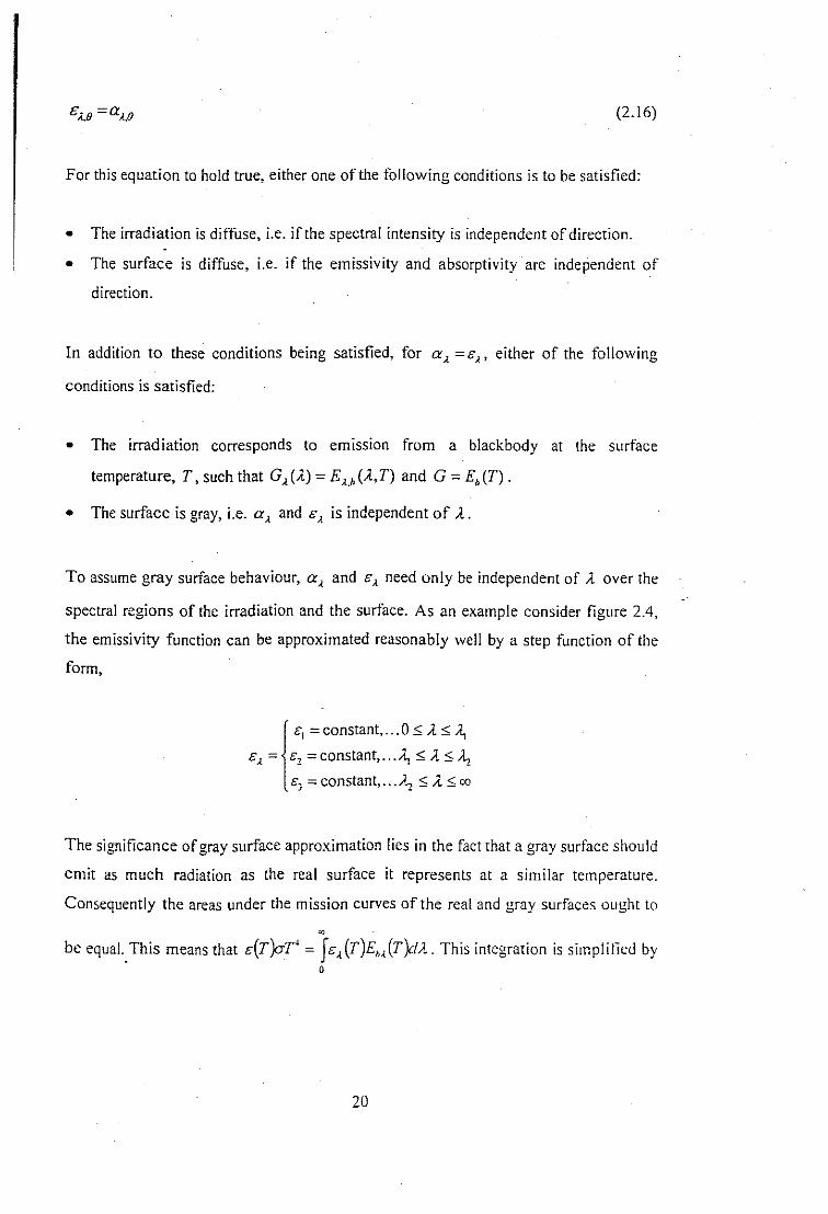
To assume gray surface behaviour, a, and c, need only be independent of A. over the
spectral regions of the irradiation and the surface. As an example consider figure 2.4,
the emissivity function can be approximated reasonably well by a step function of the
form,
101 =constant, 0 CS; A CS; A,
c, = 0, =constant, A, CS; A CS; A,o. =constant, A, CS; A CS; Cl)
> •
The significance of gray surface approximation lies in the fact that a gray surface should
emit as much radiation as the real surface it represents at a similar temperature.
Consequently the areas under the mission curves of the real and gray surfaces ought to
~
be equal..This means that o(T)aT' = Jc,(T)E,,(T)dA. This integration is simplified byo
20

r-- /':c2 '-..../
Real surfacevariation
Cl r--- /V '-----" j~
c,
!
A ~r-- ,
V
A, A., A
Figure 2.4 A pproximating a real surface emissivity variation with wavelength
by a step function.
separating the spectrum into a number ofwavelength bands and assuming the emissivity
remains continuous over each band. The average emissivity can be determined from the
definition of blackbody radiation.
J. 1 1 2 :(C
cIJE.,CT)dA Ii,JE.,CT)d,l c,JE"CT)d,lcCT) = 0 + _;e,"'_-::::--;;-__ + _-,,",-,---;-__
~T4 ~T4 ~T4
2.3 Geometric considerations
(2.17)
In many industrial applications the exchange of radiation heat transfer between different
solid surfaces is unaffected by the medium separating them. This is a common
OCcurrence since air and most gases are termed as nonparticipating media. Since such
media neither emits, absorbs nor scatters. it does not affect the transfer of radiation
between surfaces. Radiative heat transfer between two or more surfaces depends to
21

some degree on their orientation relative to each other, size, separation distance and
temperature.
Calculations in radiative heat transfer are simplified by only considering the geometric
features of the surfaces involved. Thus neglecting the effects of surface temperature and
surface properties. Performing a radiation analysis on surfaces based on the effects of
orientation alone is termed as the view factor. View factors considered here are based on
the assumption that the surfaces are diffuse emitters and diffuse reflectors, hence dijfilse
view factors. Specular view factors are not considered in this study. Performing a
radiation analysis for one surface requires that all surfaces that can exchange radiative
energy with one another be considered simultaneously.
Consider the two surfaces in figure 2.5. The view factor, Fij' is defined as the fraction
of the radiation leaving surface i that is intercepted by surfacej directly. Mathematically
the view factor is described by the double integral of equation (2.18).
I J JCos Bi cos BjFij =- , dAidA JAi 'A trR-., ,
(2.18)
The values for the view factor are a numerical constant between zero and one. Some
special conditions are be presented here (<;:engel, 1997):
• The view factor from a surface to itself will be zero for a plane or convex
surface, i.e. F" =0 . However for concave surfaces, F" ;t 0 .
• If surface j completely surrounds surface i, so that all the radiation leaving
surface i is intercepted by surface j, then F" =I .
• When two surfaces do not have a direct view of each other, such that radiation
leaving surface i is unable to strike surface j, Fij = 0 .
22

Figure 2.5 Radiative exchange between two elemental $Urf.lces.
2.3.1 View factor algebra
When studying the view factors for various surfaces and orientations, it useful to
consider these as relating to an enclosure. The analysis however would require the
evaluation of N' for an enclosure consisting of N surfaces, which is neither practical
nor necessary. This approach however is computationally intensive, but by utalising
some fundamental relations for view factors, simple geometries are solved for.
2.3.1.1 The reciprocity rule
AF =A FI IJ .J]I
(2.19)

This enables the determination of the counterpart ofa view factor by knowing the view
factor itself and the areas of the two surfaces.
2.3.1.2 The summation rule
(2.20)
In an enclosure the conservation of energy principle stipulates that the entire radiation
leaving any surface i within, be intercepted by the surfaces of the enclosure. The
definition given in equation (2.20) is expressed as the sum of the view factors from
surface i ofan enclosure to all surfaces of the enclosure, including itself must equal
unity.
2.3.1.3 The superposition rule
If a view factor to be determined for a certain geometry is not available in the standard
tables and charts, the superposition principle is lIseful. The view factors of known
geometries are added or subtracted so as to closely approximate the required geometry.
Consider the geometry of figure 2.8, the rule can be expressed as follows: the view
factor from slIljace i to a surface) equals the sum ofthe view factors from surface i to
parts ofsurface j.
A mathematical relationship is given in equation (2.2 I).
F -F 'Fi(j,k) - ij T Ik (2.21)
This rule is however not reversible such that the view factor from a surface) to a surface
i is not equal to the sum of the view factors from surface) to parts of surface i.
24

k
i
i
;
k
i
Figure 2.6 The view factor from a surface to a composite surface
2.3.1.4 The symmetry rule
Further simplification in the determination of a view factor is possible if the geometry
involved possesses a degree of symmetry. Expressed as follows: two or more slIr/aces
that possess symmetry about a third surface will have identical view factors from thal
surface. If surfaces j and k are symmetric about surface i the following holds true:
(2.22)
This relation is also true for the rule of reciprocity.
View factors for many conventional geometries are analysed and evaluated in several
publications. These derivations include results for two and three-dimensional
geometries.
25

2.4 Radiation heat transfer between black surfaces
Radiation may leave a surface due to both emission and reflection. The investigation of
radiation exchange between surfaces, in general, is complicated because of reflection: a
radiation beam leaving a surface may be reflected many times, with partial absorption
occurring at each surface, before it is finally absorbed. The analysis is greatly simplified
if the surfaces involved can be approximated as blackbodies, because of the absence of
reflection.
The net rate of radiation heat transfer between two black surfaces of arbitrary shape and
maintained at uiliform temperatures T, and Tj
is given by the relation (2.23).
(2.23 )
Applying the reciprocity rule to (2.2 I) it yields,
(2.24)
The net radiation heat transfer can also be defined as, qij =q" -qj" if q'j is negative
then the net radiation heat transfer is to the surface, i.e. surface i gains energy instead of
losing. For an enclosure consisting of N black surfaces maintained at specified
temperatures, the net radiation heat transfer from any surface i to each of the surfaces in
the enclosure can be expressed as,
q, = Iq'j = IA,FijO"(:r,4 -T/)I=I j:::l
2.5 Radiation heat transfer between diffuse, gray surfaces iu an enclosure.
(2.25)
Radiation exchange formulae are available for blackbodies, because these results can
differ considerably from the practical realisation; its usefulness is generally limited to
26

analytical analysis. A blackbody is an idealisation that can be closely approximated by
some surfaces, but is never accurately achieved. Calculations involving real non
blackbody surfaces do present increased mathematical complications; therefore these
calculations invariably assume certain conditions. The calculations involved in
analyzing radiation exchange can be simplified by making certain assumptions. These
conditions include:
• The surfaces of the enclosure are isothermal, which IS indicated by a uniform
radiosity and irradiation.
• Surface behaviour is opaque, diffuse and gray.
• The medium within the enclosure is nonparticipating.
The aim of many calculations is to determine the net radiative heat flux qi' knowing the
temperature T, associated with each surface of an enclosure. The radiosity J is defined
as the total diffuse energy leaving a surface through emission and reflection. Where the
radiosity of a blackbody is given by: J = Eh =aT' . Such that its radiosity equals its
emissive power since it does not reflect any radiation.
For a surface i that is opaque, diffuse and gray (G, =a i and a, + r, =I), the radiosity is
expressed as:
J i =(radiation emitted by surface i) + (radiation reflected by surface i )
= G;Ebi + 'iGj
= G,Eh, + (I - G, 'pi
27
(2.26)
2.5.1 Net radiation heat transfer at a surface
The effect of radiative interactions at a surface determine whether a surface losses
energy or whether it gains energy. A surface loses energy by emitting radiation and
gains energy by absorbing radiation emitted by other surfaces. Depending on which
quantity is greater a surface will experience an overall gain or loss of energy.
The net rate at which radiation heat transfers from a surface i of surface area A, given
as g;. is expressed as:
g, = (radiation leaving entire surface i) - (radiation incident on entire surface i)
=A,(J, -G,)
(Eh, -J,)=(l-.o,)/
.-'ciA;
(2.27)
Depending on the relative magnitudes of the radiosity (J,) and the emissive power of a
blackbody at the temperature of the surface (Eh')' the direction of the net rate of heat
transfer is determined. If Eh, > J" the direction is from the surface and if Eh, < J" the
direction is to the surface. If g, is negative, it indicates that the heat transfer is to the
surface.
2.5.2 Net radiation heat transfer between surfaces
The net rate of radiation heat transfer from surface i to the sum of the surfaces involved
in the radiative exchange can be expressed as the following:
[
radiation leaving entire] [radiation leaving entire]q" = surface i that - surface j that
strikes surface j strikes surface i
28

N
= LA,Fij(J,-JJj=l
2.6 Methods of solving radiation problems
(2.28)
When an analysis of the radiation of an enclosure is performed, either the surface
temperature, T" or the net rate of heat transfer, q" must be known for each surface.
This is necessary to obtain a unique solution for the unknown surface temperatures and
heat transfer rates.
The conservation of energy principle requires that in an N-surface enclosure, the net
heat transfer from surface i be equal to the sum of the net heat transfers from surface i to
each of the N surfaces of the enclosure. The relation that describes this principle is given
in equation (2.29).
(2.29)
This relation is especially useful when the net radiation heat transfer rate, q, is known.
However this may not always be the case. Typically the situation exists that the surface
temperature, T, (hence Eh;) is known and equation (2.30) proves more useful. This
equation is a combination of equations (2.27) and (2.29), which is given as,
(2.30)
The equations (2.29) and (2.30) give nse to N linear algebraic equations when
determining the N unknown radiosities for an N-surface enclosure. After determining
the radiosities J"J" ...,JN the unknown surface temperatures and heat transfer rates are
29

derived from equations (2.29) and (2.30) respectively.
The matrL, method is a direct means of solving radiation heat transfer problems. These
problems typically involve the use matrices especially when many surfaces are engaged.
The use of iteration or matrix inversion to solve a problem involving any N number of
surfaces may be obtained by rearranging equation (2.29) or (2.30) to get the following
system ofN equations:
[A][J] =[C]
°If···Qli···QIN J, C,....................
....................
where: [A] = aU···a1i···QIN [J]= J, [C]= C,
....................
....................
all,··Qli···QIN I N CN
..........................................
..........................................
..........................................
..........................................
30
where:
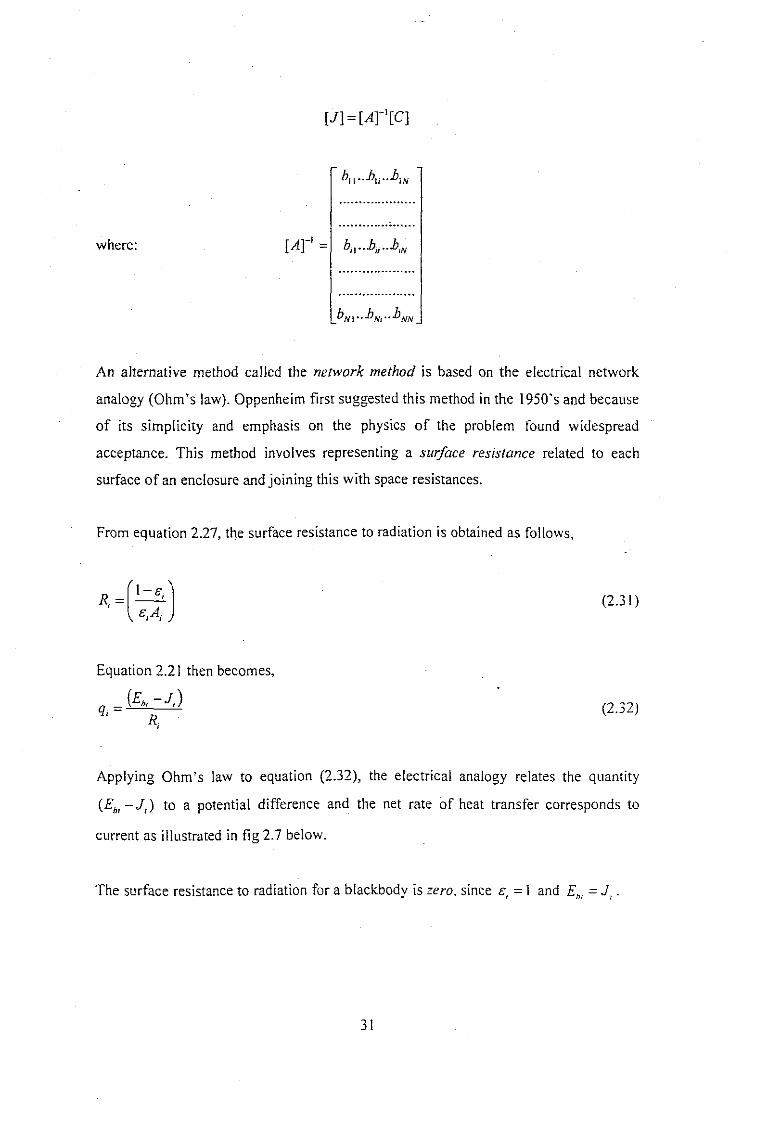
An alternative method called the network method is based on the electrical network
analogy (Ohm's law). Oppenheim first suggested this method in the 1950's and because
of its simplicity and emphasis on the physics of the problem found widespread
acceptance. This method involves representing a surface resistance related to each
surface of an enclosure and joining this with space resistances.
From equation 2.21, the surface resistance to radiation is obtained as follows,
Equation 2.21 then becomes,
q = (E.,-J,), R,
(2.3 I)
(2.32)
Applying Ohm's law to equation (2.32), the electrical analogy relates the quantity
(Ehi -J,) to a potential difference and the net rate of heat transfer corresponds to
current as illustrated in fig 2.7 below.
The surface resistance to radiation for a blackbody is zero, since G, =1 and Eh, =J, .
31

q,
~ J,
Surface i
Figure 2.7 Electrical analogy of surface resistance to radiation
A real surface can be modelled as being adiabatic, if one of its sides is well insulated
and the effect of convection on the other side is negligible and steady-state conditions
are achieved, the net rate of heat transfer though the surface is zero. This means that the
surface looses as much energy as it gains. Such a surface is known as·a reradiating
surface and from equation (2.32) setting q, = 0 yields the following:
J =E. =aT4, , , (2.33)
The temperature of a reradiating surface is independent of its emissivity. The surface
resistance of a reradiating surface is neglected because there is no net heat transfer
across it. (Similar to the electrical analogy if there is no current through a resistor it can
be neglected.)
The space resistance is obtained from equation (2.28) and expressed as,
(2.34)
Equation 2.28 then becomes,
32

(2.35)
Repeating the Ohm's law analogy in equation (2.28), V, - JJ relates to a potential
difference and the net rate of heat transfer between two surfaces correlates to current as
shown in figure 2.8.
When applying the network method it is generally limited to simple enclosures i.e.
enclosures consisting of three or four surfaces, due to the increased complexity of the
network.
Surfacej \
. Eb}
» J,
R=_l_ij AF
, lj
J,
Eh,
Surface i
Figure 2.8 Electrical analogy of space resistance to radiation
33

2.7 Radiation heat transfer in two-surface enclosures
The simplest example of an enclosure is one consisting of two opaque surfaces at
individual temperatures 1; and T" that exchange radiation only with each other as
illustrated in fig 2.9. The net rate of radiation heat transfer from surface I, q" should
equal the net rate of radiation heat transfer 10 surface 2, - q" and furthermore the sum
ofthese quantities should equal the rate at which radiation heat is transferred between I
and 2, expressed as, q, = -q, = ql2.
£,
A,T,
q, ql2 q,
• J, • J, •Eh, Eb ,
R _I-c, 1 R _I-c,,- R,.,::::-- , -A,c, . A,F" - A~£2
Figure 2.9 Schematic of a two-surface enclosure and the radiation network
associated with it.
34

The network representation of this enclosure consists of two surface resistances and one
space resistance, as shown in fig. 2.9. When determining the electrical current through a
series of resistances in an electrical network, the potential difference across the total
resistance is divided by the sum of these resistances. The net rate of radiation heat
transfer is obtained in a similar manner, and may be expressed as
(2.36)
This significant result may be used for any two diffuse, gray, opaque surfaces that form
an enclosure. The geometry of the enclosure determines the view factor F". Table 2. I
below summarises some special cases where F" =1.
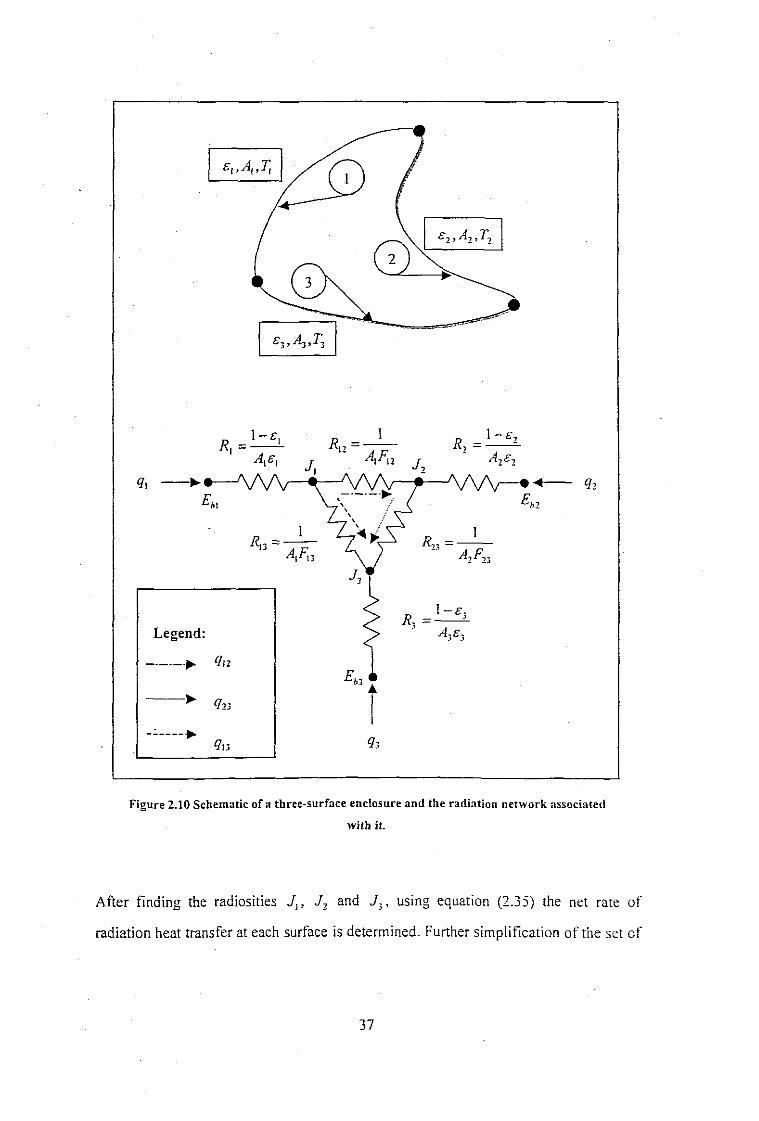
2.8 Radiation heat transfer in three-surface enclosures
For an enclosure constituting three opaque, diffuse, gray surfaces, as depicted in fig.
2.1 0, with the surfaces having respective emissivities, surface areas and uniform
temperatures, the network of this geometry is evaluated by representing surface
resistances for each of the surfaces and joining these with space resistances, as
illustrated in fig. 2.11. If the surface temperatures are known, the end-point potentials
E", E" and E" are then simply derived. The radiosities JI , J, and J, are solved
from the condition that the algebraic sum ofthe currents (net radiation heat tramJer) at
each node must equal zero. The set of equations obtained from this requirement that
need to be solved for are given below.
EhJ -JI J, -JI J, -JI °-"'---'-+ - + -'---'-RI RI, RI'
JI-J, + E" -J, + J, -J, 0
Rn R2 Rn
JI-J· J,-J. Eh·-J· 0-'-_"--'+ .l+:t-'
RI3 R23 R3
35
(2.37)

Table 2.1 Special Diffuse, Gray, Two-Surface Enclosures
Large (infinite) Parallel Planes
/ I A"T"c, IA, =A, =A and
Ao-(:r,' - T,' )1 1-+--1Cl c2
F" = 1
(2.3 7a)
F" = 1
Long (infinite) Concentric Cylinders
Qand
(2.37b)
Concentric Spheres
GJAI r,,2-=---:;A
2r
2-
and F,,=!
(2.37c)
F,,=l
Small Convex Object in a Large Cavity
36
and
(2.37d)
~.A"T. \
3
q,
Legend:
_._._-~ q,z
-----~
Figure 2.10 Schematic of a three-surface enclosure and the radiation network associated
with it.
After finding the radiosities Jp Jz and J" using equation (2.35) the net rate of
radiation heat transfer at each surface is determined. Further simplification of the set of
37

equalities in equation 2.37 is possible if one or more surfaces exhibit blackbody
behaviour such that J i := Ebi := aTi or ifone surface is reradiating then q, =O.
2.9 Radiation shields
Sometimes it may be necessary to reduce the net radiation heat transfer between two
surfaces using a radiation shield that is constructed of material with a low emissivity
(high reflectivity). This material inserted between the two surfaces diminishes the rate
of radiation heat transfer by introducing additional resistances in the path of radiation
heat flow. A shield with a low emissivity represents a high resistance.
Equation (2.37a) represents the radiation heat transfer (with no shield) between two
large parallel plates with emissivities c. and cz sustained at uniform temperatures T,
and Tz • If a radiation shield were inserted between these two plates as depicted in fig.
2.11, the resultant net rate of radiation heat transfer is given by equation 2.38.
The emissivity associated with one side of the shield (c, .• ) may differ from that
associated with the opposite side (cJ.2) and consequently the radiosities will di ffer.
Applying the network method to this geometry and recognizing that F" = F'", = I , also
that A. := Az = A3 = A for parallel plates an expression for the net rate of radiation heat
transfer is simplified as shown below.
(238)
The equilibrium temperature of the shield, T" is determined frpl1l the fact that at stcady-
state conditions g" = glJ = g3Z and expressing equation (2.37a) for q" or q,z' For a
configuration consisting of N radiation shields the net rate of radiation heat transfer is
expressed as:
38

(I) Shield (2)
T, T, T, T,
Cl c3.1 0'_ , 0',>.-
.. ..qJ2 ql' q12
I-cl 1-0'-1 1-0'" 1-0',>, ----Cl Al AIF" C3.I A3 G3,lA] A3F;z GzA2
A A AA A A A AA N if- Vvv Vv vvv VV
E bl Eh2
Figure 2.11 The radiation network associated with a radiation shield
placed between two parallel plates.
(~+~_I)+(_I+_,_1)+ ...+(_1+-'-I)\. £, El E:U £3,2 eN.! EN.2
(2.39)
For the special case when the emissivities of all the surfaces are equal, equation 2.39
becomes,
39
(2.40)

2.10 Participating Media
The means developed thus far for predicting radiation exchange between surfaces has
inherent restrictions. We have considered isothermal, opaque, gray surfaces that emit
and reflect diffusely and additionally also characterized by uniform surface radiosity
and irradiation. For enclosures, the medium separating them was considered
nonparticipating or transparent, which means it neither absorbs nor scatters the surface
radiation and emits no radiation of its own, it does not participate in the heat transfer
process.
The equations based on the preceding assumptions in most instances provide highly
accurate results for radiation heat transfer in an enclosure. This is the case when the
space separating the radiating surfaces is occupied by vacuum or by a gas with
monatomic or symmetrical diatomic molecules (nonpolar). The gases that satisfy this
criteria include the following; the main components of air (N 2 , °2 ), H 2 , Ne, Ar and
Xe. There are times however when the preceding assumptions are inappropriate because
the separating medium scatters or absorbs radiation passing through it and emits
radiation of its own. Examples of these types of media are strongly polar gases such as
CO 2 , Hp (vapour), NH3 , S02' hydrocarbons and alcohols.•
Gaseous radiation as opposed to radiation from a solid or liquid is not a surface
phenomenon but characterized by a volumetric absorption, transmission and emission of
radiation. Gaseous radiation is concentrated in specific wavelength intervals or bands.
Radiation with a wavelength outside these bands will pass unattenuated through the
medium and with respect only to this radiation the medium is nonparticipating.
Spectral radiation absorption in a gas (or in a semitransparent liquid or solid) is a
function of the thickness L of the medium and the absorption coefticient K A • which has
units m-I. If a monochromatic beam of intensity 1•.0 is incident on the medium, the
intensity is reduced due to absorption. Beer's law, equation 2.41, is a useful tool in
40

approximate radiation analysis and may be used to infer the overall spectral absorptivity
of the medium.
(2.41 )
The transmissivity of the medium is defined as,
(2.42)
and the absorptivity of the medium is given as,
(2.43)
In addition if the temperature of the gas T. is uniform and does not differ noticeably
from the temperature T. of the surface that produced the beam of intensity 1l.O' we may
assume Kirchoffs law as valid such that,
(2.44)
2.10.1 Gaseous Emission and Absorption
A method to determine the radiant heat flux from a gas to an adjoining surface was
developed by Hottel (1954). This is a simplified procedure that involves determining
radiation emission from a hemispherical gas mass of temperature T., to a small area
A" which is located at the center of the hemisphere's base. The radiation heat rate that
is emitted by the gas and arrives at A, is,
(2.45)
41

The gas emissivity lig is obtained by correlating data in terms the temperature T., the
total pressure P of the gas, the partial pressure Pg of the radiating species and the radius
L of the hemisphere. This result is sufficient when the gas mixture consists of one
radiating gas for instance water vapour or carbon dioxide and other nonradiating
species. However when two radiating gases appear together in a mixture with other
nonradiating gases, the total gas emissivity may be expressed as,
(2.46)
The correction factor 1'>E given in available literature for different values of the gas
temperature, accounts for the reduction in emission associated with the mutual
absorption of radiation between the two gases. If the surface surrounding the gas is
black, it will naturally absorb all the radiation that is emitted by the gas. The net rate at
which radiation is exchanged between the surface at T, and the gas at Tg is given as,
(2.47)
The total gas absorptivity when both water vapour and carbon dioxide are present may
be expressed as, a. =a" +a, - 1'>a , where 1'>a =1'>E .
In order to calculate the required gas absorptivity a g of either water vapour or carbon
dioxide the following expressions are given by Hottel (1954).
Water: (2.48)
Carbon Dioxide:
42
(2.49)

3. CONTROLLER DESIGN
3.1 Mathematical modeling and experiments
The aspects of modeling in an IR system usually concern either the IR lamp or the
industrial application. Infrared dryers are an integral part of many commercial
enterprises and infrared drying an essential process for many businesses in
manufacturing. Studies of infrared drying kinetics and drying phenomena are limited,
but there are several publications concerning heat and energy transfer in infrared dryers
and some are presented below.
3.1.1 Overview of infrared drying studies
The studies available are limited to applications involving paint, foodstuffs and
continuous sheets of paper and textiles. An experimental study performed by Parouffe el
a! (1992) on the combined effect of infrared and convective drying of glass beads
investigated the drying characteristics and the influence of thermal radiation on
convective heat and mass transfer. Drying experiments performed by Navarri el al
(1992) on a wet sand layer subjected to intensive infrared radiation were analysed and a
simple model was developed, able to predict drying rates and surface temperatures. A
further model resulted from experiments by Navarri and Andrieu (1993), delivered a
model that is able to predict drying rates and temperature profiles down to zero moisture
content. Studies on infrared drying characteristics of wet porous materials in
comparison with convective drying results conducted by Hashimoto and Kameoka
(1998) used three kinds of membrane filters with differing mean pore diameters.
A method for the calculation of the drying time and surface temperature of water based
paints during both convective and infrared drying was presented by Silventoinen and
Palosaari (1982). The model integrated mass and energy balances with an experimental
characteristic-drying curve. Rosier et a! (1995) performed drying experiments with
water-based paints and organic coatings using infrared heaters with various emission
spectra. In the experimental work of Blanc el a! (I 997a) they presented some models
43

relating convective and infrared drying of reactive automotive paints. These paints are
sensitive to the vaporization process and are coupled with a polymerization reaction in
the paint film. Experimental and modeled drying curves were presented and techniques
for monitoring the reaction and drying kinetics were discussed. Methods for studying
the reaction kinetics during the infrared curing of epoxy-based automotive paints were
developed by Blanc et al (1997b) along with related changes in structure and in
rheological behaviour.
An investigation by Le Person et al (1998) on the drying of a thin multi component film
produced for pharmaceutical purposes. Measurements of the internal concentration
gradients and the results were combined with drying rate data in order to obtain a better
understanding of the drying process and of the multicomponent transport phenomena
involved. With this information they were able to explain and prevent the occurrences
of mechanisms detrimental to product quality.
An analysis of an application of infrared drying in food manufacturing by Sandu (1986)
discussed transport phenomena and process applications. Yamasaki et al (1992)
investigated the infrared drying of food through the use of gelatinous materials as mqdel
substances. Numerous factors that influenced drying rate and shrinkage as well as the
radiative properties of the product and heater were examined experimentally and were
compared to with a simple drying model. A set of heat and mass transfer equations were
proposed by Fasina et al (1998) to simulate the infrared drying of agricultural crops. A
comparison was made with the model and experimental data on the surface temperature
and average moisture content of barley kernels found on a vibrating conveyor exposed
io infrared radiation. More drying experiments performed by Afzal and Abe (1999) used
an infrared heater to investigate the drying characteristics of potato slices. They
investioated the effects of several parameters on drying rate and product temperatureo
history.
An investigation by Broadbent et al (1994) on the many parameters that influence
drying rates when a number of different textile fabrics were pre-dried in a pilot scale
infrared dryer. In another study Dhib et al (1994) proposed a transient model, a set of
44

partial differential equations, for the infrared drying of continuous thin sheets and
calibrated the model by using data from a large number experiments on an infrared
textile dryer. Experiments on varying conditions were investigated and the model
predictions were found to be in good agreement with the experimental data. In another
paper by Dhib et al (1998) these equations were analysed for controllability and
observability after being reduced to a model adaptable to direct control. The aim of the
model reduction contributed to the design of a model based controller for an infrared
dryer.
Modeling experiments by Heikkila (1993) on the drying of coated sheets of paper by
infrared dryers proposed separate balance equations for the base sheet and the coating
layer. The radiation energy was assumed to be evenly absorbed throughout the thickness
of the sheet and was treated as a source term in the energy equations. Drying
simulations by several techniques based on the model were used in a pilot machine and
model predictions compared well with experimental results.
In reference to infrared drying in general considering the limited literature available this
is an area in which there is a need of considerable research efforts. This is especially
important in view of the many industrial applications possible with infrared radiation.
3.1.2 Mathematical models of electric IR heaters
Numerous models ofgas-fired IR heaters have been presented in a number of studies in
available literature. The models available range in complexity from very simple
radiation exchange models to advanced models dealing with combustion and transport
phenomena in porous media.
With respect to electric IR heaters, very few models are available. Some work regarding
radiation exchange modeling in electric heaters has been conducted in studies
concerning infrared paper drying (Lampinen et al., 1991 ;Ojala et al., 1995). The type of
IR heater modeled in this case is of the glass enclosed metal filament type. The models
they developed in-elude non-gray radiation heat transfer "between the filament, the
45

reflector, the protective glass, the paper sheet and the back reflector. The radiative
properties of some of the components were measured using an integrating sphere in the
range 0.4 - 201-'J1!. A related model was later developed by Pettersson (1998), which also
incorporated the lamp glass in order to validate the spectral distribution of an electric IR
heater, similar to that of figure 2.3.
An assumption made was that the temperatures of the various components were known
and was used as input data for the model. A further assumption was that all the
electricity supplied was converted to radiation at the filament (Penersson, 1999).
Because these models assume the temperature of the heater components to be known,
they consequently do not characterise heater models completely. In their opinion Ojala
and Lampinen caution that their results can only be regarded as quantitative, because the
temperatures involved in their assumptions represent a wide margin of ambiguity. In
addition Pettersson (1999) further elaborates that since the approach in the models
developed utilised assumed temperatures, these results could possibly lead to
impractical consequences with regard to the energy balances considered.
3.2 Overview of process control aspects
3.2.1 Mathematical description of a control system
A block diagram of a general control system in the Laplace domain is shown in figure
3.1 below. The feed forward transmission path transfer function is given by G(.;); Hr.,)
represents the feedback path transfer function. Typically the feedback element contains
the sensor or transducer that measures a physical quantity, such as temperature and
converts this measurement into a voltage. H(s) therefore represents the gain of the
sensor. The basic idea in many control systems is to make the controlled output, c(t),
follow the reference input, rU), as closely as possible. Therefore the desired transfer
function is:
46

R(s)I
£(s) C(s)---,~
G(s)r(!) - er!) c(1}
H(s)
.
Figure 3.1 General analog control system
T(s) = C(s) = 1R(s)
(3.1 )
If r(t) varies with time, then the problem is commonly referred to as a tracking
problem. However if the input remains constant, it is known as a regulator problem. If
the output, C(s), is not measured, H(s) = 0 and the system is open loop. Disturbances in
the feedforward transmission path usually compound the problem of making c(t)
follow r(t). Neglecting any disturbances, figure 3.1 illustrates the closed loop feedback
system since the controlled variable is measured and used to control the system.
An expression for the error for the system is given by £(s) = R("j - HMC("j. However
C(s) = G("j£(s). Solving these two equations the closed loop transfer function is:
T(s) =C(s) = G(s)R(s) I +G(s)H(s)
(3.2)
With the addition of a controller to the forward transmission path of the control system,
as shown in figure 3.2 the error in the system is diminished. A controller compares the
actual value of the plant output, CrI), with the reference input, r(l}, which is the desired
value, then determines the deviation or error and produces a control signal that will
reduces the error to zero or a small value.
47

G(s)
+R(s) £(s) U(s) C(s)
Ge(s)• Gp(s)
r(l) --, e(l) "(I) C(I)
H(s)
-
Figure 3.2 General feedback control system with compensation
The transfer function of the control system as depicted in figure 3.2 with unity feedback,H(s) = 1, is expressed as:
(3.3)
The input to controller is the error signal, £(s), and the output of the controller, U(sj, is
the input to the plant under control, GI'(s). Again the purpose of the controller is to
ensure the output follows the input so that the condition in equation 3.1 is satisfied.
3.2.2 PID control of the plant
In practical temperature control applications, the problem or difficulty is the incidence
of thermal time lag, which leads to conditions such as overshoot and temperature
cycling. These effects are of acute importance when the product being processed or
heated is temperature sensitive and in danger of being damaged in this way. While lag is
usually unavoidable in a practical process, there are ways of limiting it.
48
For accurate control of the load temperature an effective controller is required. A closed
loop proportional integrated controller (PID) satisfies this need by providing a stable
regulated temperature control. It is well known that temperature loop dynamics can be
slow because of process heat transfer lags, which is the case in medium and long wave
infrared heaters. Short wave infrared heaters, quartz glass enclosed tungsten filament
type, usually reach final temperature, typically between 2000°C and 2500"C, within a
few seconds. Medium and long wave heaters, ceramic encased electric heating coil type,
have heating constants in the order of minutes. Their maximum temperatures typically
range from 600"C for long wave and 90Q"C for medium wave heaters. The slower
heating constants for medium and long wave heaters imply the presence of significant
dead time. Coupled with the fact that temperature systems are not normally noisy, PlO
control is usually preferred.
For optimal performance the type of heater chosen for a system should be one that has
a low thermal mass (fast reaction time) or the temperature sensor employed should have
a fast reaction time. Optical sensors when compared to other forms of sensing, such as
thermocouples, provide the quickest temperature measurements and are consequently
the type used in this paper. The PID controller required in order to satisfy the above
criteria should be capable of reducing the heater power well ahead of the temperature
reaching set point. This means that the power has to be minimised in proportion to the
distance from the set point. This way the controller is capable of preventing temperature
overshoot and cycling. This action describes it as a proportional controller (P). The
relationship between the output of the controller and the actuating error signal is,
(3.4)
If the gain Kp
' is high, the slightest error signal e(t), results in a dramatic change in the
output !t(t). With an increase in gain the rise time is reduced allowing the outp\lt to
rapidly follow the input. When the proportional band, the range of error possible, is
wide the output can be diminished sooner avoiding overshoot, but a temperature offset
is usually the result. To maintain the temperature about the set point as accurately as
possible, very often a manual reset ofthe control parameters is needed.
49

To automatically and continuously adjust the temperature by adjusting the power input,
an integral action is needed. The controller needs to make the power increase in
proportional to the deviation from the set point, so that the steady-state error is reduced
to zero. The steady-state error is that deviation between system output and input after
transient effects have died away. This is type of control is expressed as integral control
and defined as,,
u(t) =K, Je(t)d(t)o
(3.5)
With the addition of this integral action the effect is a proportional + integral controller
(PI), defined as,
K'u(t) = K pe(t) +--.!'.. Je(t)d(t)
1'; 0
(3.6)
The output, u(t), is controlled by adjusting the proportional gain, K p and the integral
time, T,.
With the addition of derivative control, the controller anticipates changes in temperature
and modifies the input power proportional to the rate of change of temperature. The
purpose of this type of action is to minimise and damp unwanted changes and speeds
recovery from temperature disturbances, which is effective during transient periods. The
ensuing controller known as proportional + integral + derivative (PID) control combines
the advantages of the three individual control actions and is defined as,
(3.7)
When a comparison of three types of controllers to a step function is made, the curves
obtained in figure 3.3 results. A step function represents a radical change in system
input, and the system response is a good indication of the controller's performance
50

0.9 (c)0.8
0]
0.6
0.5
0.2
0.1
0.250.20.150.10.05
o1 L-__..L__...L__--'-__-.L__--.-J
o
Figure J.J Step response of a closed loop feedback system shown for (a) P controller,
(b) PI controller and (c) PID controller
when subjected to a disturbance. The PID controller clearly provides the most stable
output ensuring that the steady-state error, e~, is diminished to zero.
If a mathematical model of the plant is not known, then it is possible to apply diverse
design techniques for determining parameters of the controller that will satisfy the
transient and steady-state specifications of the closed-loop system. The simplest
approach in the design of PID controllers is an experimental one.
The process of selecting the controller parameters in order to obtain the required
performance conditions is known as controller tuning. Ziegler-Nichols proposed rules
for determining values of the proportional gain K p , integral time r. and derivative time
Td
, based on the transient response characteristics of a given plant (Leigh, 1988). The
transfer function G,(5) of the PID controller is given as:
(3.8)
51

3.3 Controller Design
3.3.1 Identification of the infrared oven (heater)
In order to obtain a mathematical description of the IR heater. a transfer function, the
method outlined below was completed. This method is the Ziegler·Nichols design
approach. Known as the process reaction. method, it requires the open-loop step
response of the process to be recorded and is a practical means of acquiring the transfer
function of the IR heater. There are two methods for Ziegler-Nichols tuning, both aimed
at obtaining 25% maximum overshoot in step response. The process reaction method
was chosen because the curve resulting from a unit-step input resembled an S-shaped
curve as depicted in figure 3.4. The type of IR heater used was a medium wave infrared
ceramic type. The S-shaped curve is characterised by tWQ constants, delay time Land
time constant T. By drawing a tangent line at the inflexion point of the S-shaped curve
and determining the intersections of the tangent line with the time axis and the line
c(t) =K, the values for the delay time and time constant are determined. The transfer
c(1)
K - _.._ _ =.:::::::::::::;;;::;:;;.=_
o
T
Figure 3.4 S-shaped open loop step response curve

function Gp(s) =C(s)/U(s) , equation 3.9, is approximated by a first-order system with
a transport lag.
G (s) =C(s) =Ke-I~p U(s) Ts+I
(3.9)
Table 3.1 indicates the suggested values for the controller parameters as described by
Ziegler-Nichols process reaction method.
Table 3.1 Ziegler-Nichols tuning rules based on step response of plant
Type ofKp T, Td
Controller
P (1i) 00 0
PI O.9(1i) (%.3) 0
PID l.2(1i) 2L O.5L
3.3.2 Experimental Results for step response of the plant
The open loop step response of the IR heater under test resulted in the curves shown in
the figures 3.5 to 3.8 below.
The curve in figure 3.8 was chosen as a reasonablt; compromise for the step response of
the plant under test. Using the Ziegler-Nichols process reaction method as described in
figure 3.4, the plant (infrared heater) was found to have an approximate transfer
function as expressed by equation 3.10.
G (s) =3.96e-"I' 140s+1
53
(3.10)

.. w: I'TJ---If--T -p
p ~ r-v". .../'
1/V i
/ ·I
W'< [ ~ .. - I .:.."
.
I·...." ..', -, , .
I :/ ' "
•
il1/I I
,•
·
V -
N - - - - - - - - - - - - - - -; 9 9 ~ 0 ~ 0 " i " 0 " 0
~ ~ g " • ~ • ~ • . ~ ~m.luc.)
,
""
""
H'"
Figure 3.5 Infrared heater warm-up curve (phase 1)
• 0 • .~ • ~ . • • .
~ ~ ~ ~ N N N " ~ " " ,lime (secl
r--r-Ti- I --/ ..,-- ---
r T -I I' .
I,
Ii
I I,"
r---v -rT , , " ' 1 I'
.---I
. V --, I '. I
I / V
I / 1-' I,
I II
I " l-+-_J I
:,
_l~_~--- --"-- - - - --- ,~' '---- -- -- -, , I
so
'"
>s,
Figure 3.6 Infrared heater warm-up curve (phase 2)
54

--1---~'-I---~---
l\z 1<' c
I ..
[0' .. N<..•••• tV'i< < <: r •.•'. i;iji•... '
l' 1« ".!Li.1<" ' .'............n. '.
.~. ..... : . '.'
...
.
""--
.'v'-v- ,
.. .. ' . . . :Iv "':'-y- - ,
ii .'....
~,
,
cc· 'r--.,
... ' ..... v-i'\..'
-J-VI.
~.
...
IL_
''0
lime (ser;l
-• ".
''0
Figure 3.7 Infrared heater cool-down curve (phase 3)
1 , r- -T-- ------""""[. I I .
I
-r'~ I./ ,I·· '.
/,./' ;
.
/' .,,
/
rT/ I
11I
•
Figure 3.8 Infrared heater warm-up curve (phase..J)
55

In order to verify the validity of equation 3.10, a simulation of the step response using
MATLAB software was performed. The simulation resulted in the curve in figure 3.9.
The trajectory in figure 3.9 is fairly accurate, but a slight adjustment of the gain, Kp
'
from 3.96 to 4.2 provides a better step response for the plant. The curve for the new step
response is given in figure 3.10.
3.3.3 Design of a continuous controller followed by discretisation
Using the Ziegler-Nichols rules as described in table 3.1 above, the coefficients of a
three-term PID continuous controller calculated resulted in the following values for,
K p ' T, and Td in equation 3.1 I. From the general form for a PID controller in equation
3.8, the expression for the continuous PID controller is given.
(3.11 )
In order to implement the controller on a digital platform, as illustrated by figure 3.11,
discretisation of the continuous expression is needed. There are various ways to do this,
but two methods dominate.
y(t)u(t)u(k)elk)e(t)
~Sampler ---. Digital
~computer DAC Plantor (ADC)
- -.- - _." ,---_ .._---
Sensor
-
Figure 3.9 Digitally controlled plant
56
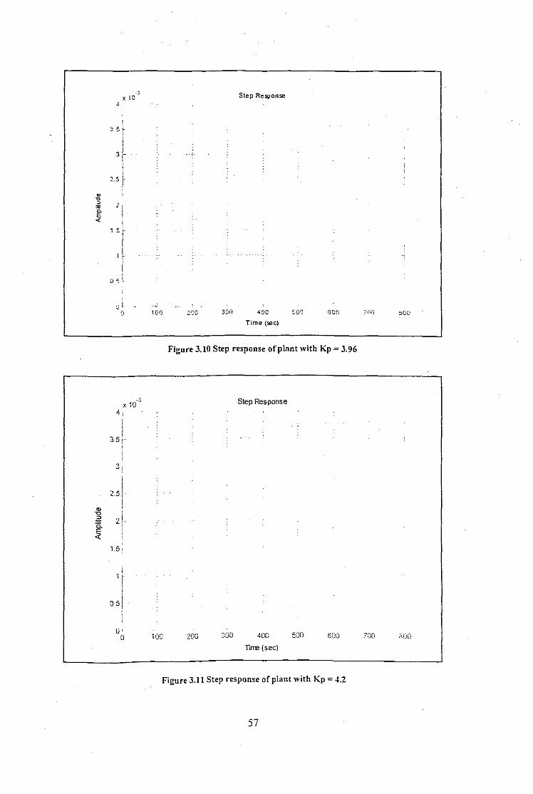
-~, ID,
3.5 rI,
3r" ._.::; ,
0u0 1s~
E<t: ,
1,
5 i·,I,
I lI,
Cl -:,~
;}LQ 1GO 300
Step Response
400
Time (sec)
GOG
x 10-~
4
35
3;
25
""0
" 2a~
1"5
05
Figure 3.10 Step response of plant with Kp = 3.96
Step Response
0'o 100 200 300 400
l1rre (sec)
500 600 700
Figure 3.11 Step response of plant with Kp =4.2
57

The first method is known as the position implementation since it controls the output ofthe controller, is given in equation 3.12. Using this method the actuator value, u" is
derived for directly.
_, KpT KpTd", -lI'_1 ,Kp(e')+T(e,)+--y-(e. -e._I)
,(3.12)
Position implementation although simple to implement suffers from some drawbacks.
When the controller is switched on for the first time, the values of "'_I and eH are not
known. The chance that by simply implementing equation 3.12 and obtaining a proper
controller output is very remote. As a result the control action of the position
implementation suffers from a 'bump'.
In addition another problem with equation 3.12 known as integral windup occurs when
the actuator encounters a constraint, which then produces a persistent offset between the
plant output and the set point. This then results in the integral term increasing without
bound over time.
Reconfiguring equation 3.12 the problems highlighted are overcome. Equation 3.13.
known as the velocity implementation, computes the increment or change of the
actuation rather than the actuation itself.
KpT KpTJ", -lI'_1 = Kp(e, -e,_I)+r(e,)+--y-(e, -2e'_1 +e,_,) (3.13)
,
The equation 3.13 produces a 'bumpless' transfer when it computes the increment of the
output of the controller. Using equation 3.11 and table 3.1 the coefficients K". T,. '(,
are solved for. The sampling period, T, is set initially to I second. The resultant
expression for the controller based on these values is given in equation 3.14.
(3.14)
58
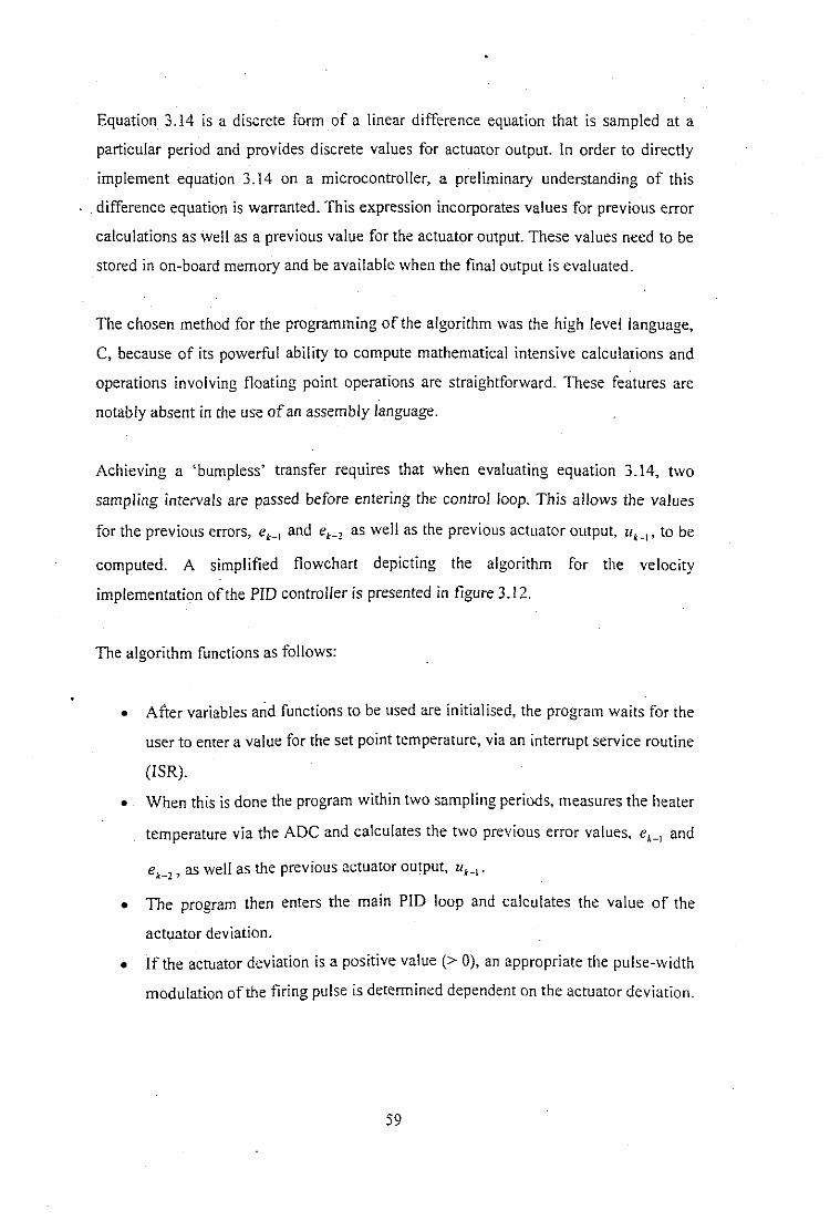
Equation 3.14 is a discrete form of a linear difference equation that is sampled at a
particular period and provides discrete values for actuator output. In order to directly
implement equation 3.14 on a microcontroller, a preliminary understanding of this
. difference equation is warranted. This expression incorporates values for previous error
calculations as well as a previous value for the actuator output. These values need to be
stored in on-board memory and be available when the final output is evaluated.
The chosen method for the programming of the algorithm was the high level language,
C, because of its powerful ability to compute mathematical intensive calculations and
operations involving floating point operations are straightforward. These features are
notably absent in the use of an assembly language.
Achieving a 'bumpless' transfer requires that when evaluating equation 3.14, two
sampling intervals are passed before entering the control loop. This allows the values
for the previous errors, e'_1 and e'_2 as well as the previous actuator output, "'-I' to be
computed. A simplified flowchart depicting the algorithm for the velocity
implementation of the Pro controller is presented in figure 3.12.
The algorithm functions as follows:
• After variables arid functions to be used are initialised, the program waits for the
user to enter a value for the set point temperature, via an interrupt service routine
(ISR).
• When this is done the program within two sampling periods, measures the heater
temperature via the ADC and calculates the two previous error values, e'_1 and
e'_2' as well as the previous actuator output, "'_I'
•
•
The program then enters the main PID loop and calculates the value of the
actuator deviation.
If the actuator deviation is a positive value (> 0), an appropriate the pulse-width
modulation of the firing pulse is determined dependent On the actuator deviation.
59

( Start )
,
rInitialise variables and functions 1
[ ISR 1 r Get set point from keypad--1 -I- --
r Sample heater temperature
l.
I Compute error
l.
r Set error = second error delay I-
r Sample heater temperature-
r Compute error- - - , -,.
I Set error = first error delay- ..- ~ -
I 1Compute first actuator output delay iI
- - -
T
60

While loopnot
terminated
Sample heater temperature
Compute error
Compute actuator increment
Terminate
Compute pulse-widthmodulation of firing pulse
Samplingdelay
N No pulse
Figure 3.12 Flowchart of the PlO algorithm
61

• If the actuator deviation is negative or equal to zero «= 0), no firing pulse is
initiated.
• The program waits for the sampling period to complete before taking another
measurement ofthe heater temperature and repeats the loop.
A complete listing of the C code for the PID controller designed is provided in the
appendix. An excerpt of the source code given below shows how the value for e'_l IS
evaluated.
Lout = ADCO; I*sample output*1
I*compute error*1
I*set error equal to second
previous error*1
The following excerpt shows how e'_1 is computed.
Lout = ADCO; I*sample output*1
1* set error equal to first
previous error*I
The value for ",_Ion start-up is derived using the source code described below.
u_old_l = 2S*error_0;
I*compute previous actuator
output*!
62

After the initialisation routine has completed the program proceeds to the main control
loop. With every sampling interval the PID model in equation 3.14 is evaluated and an
increment of the actuator output computed. An excerpt of the source code used to
achieve this is given below.
while(!RI){
I*sample output*1
error 0 = (r in - y out);- - -
u3 = 21 *error_2;
u = u1 + u2 + u3 + u_old;
I*compute error*1
I*compute actuation*1
1* The computation of the incremental actuator output *1
The implementation of the PlO controller designed for this paper is based on the
Ziegler-Nichols method and represents a significant simplification when compared to
some of the other methods available. Especially considering that the system derived for
the plant was a first order model plus lag. Other tuning methods available are:
• The trial and error method, whereby the tuning parameters are tweaked and
continually adjusted. This method is usually reserved for experienced control
engineers.
63

• Graphical design methods, which include the root-locus, Nyquist and Bode
plots. These methods are usually reserved for higher order systems.
The Ziegler-Nichols tuning method was selected because it is the oldest and most
established method available. It is also much more simpler to implement than the other
methods listed above. Many modifications of the controller developed are possible and
probably warranted in some instances. However, for the purposes required of this
controller in this study, the design proved adequate as the tests performed in chapter
five verify. Chapter four presents an overview and the practical development of the IR
controller.
64

4. PRACTICAL DEVELOPMENT OF THE IR CONTROLLER
The practical procedure for obtaining the mathematical model of the controller in
chapter 3 is explained in this section. The description that follows includes various
hardware and software aspects that constitute the practical set-up of the experiment.
4.1 Hardware set-up
Figure 4.1 shows the block diagram of the open loop response test. The hardware
component for the experiment consists of the microcontroller (80C515); a power
Micro-Controller(80C515)
- .-
V;
ElectronicPower
Controller
InfraredHeater
(ceramic)
TemperatureSensor
(pyrometer)
V;,..
DataAcquisition(Daqpad)
Figure 4.1 Elements of the open-loop step response test
controller, to modify the power input to the IR heater (oven) and a temperature sensor.
pyrometer, to measure the output temperatures of the IR heater. The data acquisition
65

successfully accomplished through the use of the National Instruments DAQPad-1200
data acquisition hardware.
4.1.1. The Microcontroller
The 80C515 microcontroller is part of 805 I family and has the following features:
• Is an 8-bit controller with 256 bytes on-board RAM,
• Eight I/O ports, three I6-bit timer/counters,
• On-board analog-to-digital converter, and
• Instruction cycle time of 600ns.
The microcontroller is used to generate a pulse-width-modulated (PWM) waveform, V:,
which is needed in order to drive the power controller, which in turn regulates the
output temperature of an infrared radiation heater.
The 80C5I5 is programmed in C and the details of the software program are given in
figures 4.7 and 4. IS.
4.1.2 The Power Controller
This unit comprises the power electronic components used to control the voltage input
for the infrared heater. The aim in using the power electronic components when
designing the power controller incorporated the following features:
•••
•
Low cost implementation
Portable hardware platform
Readily software programmable
Provide reliable results with minimum hardware complexity
66

4.1.2.1 AC Power control aspects
AC power control has undergone somewhat of an evolution when considering the
various methods in which this was achieved. The control of voltage and current has
always presented the engineer with a challenge but few options. Control circuits today
employ the use of some solid-state devices and techniques. Prior to this the most
frequent method to control large amounts of voltage involved the use of one or more
transformers. The control of large currents meant the use of large variable resistors.
rheostats, placed in series with the load being controlled. These methods of control
proved expensive, demanded high maintenance and were inefficient.
Three types of power control methods have been investigated for this paper, with the
aim being to find the most appropriate type of control for the type of load required. The
power controller needs to be able to control and switch large loads, typical currents of
up to 10 amps and loads rated for 800 watts. The types of electronic devices used for
power control that were studied are as follows:
• The triac
• The insulated gate bipolar transistor (IGBT), and
• The solid-state switch (SSS)
4.1.2.2 The Triac
Today the popular method to control large amounts of voltages and currents is by means
of thyristors and has proved very successful. These types of solid-state power devices
developed by General Electric Research Laboratories have been around since 1957.
Initially the chosen technique of power control intended for work on this paper involved
the use of a triac. The triac and silicon controlled rectifier (SCR) have traditionally been
used for various types of control including general-purpose power supplies, AC and DC
variable-speed motor drives, stepper motor control, servo motor control and light
67

dimming. These semiconductor devices offer advantages that include high reliability,
extremely fast response, selectable control parameters and low maintenance. The triac is
able to switch both the positive and negative half cycles of an ac input by simply
controlling a small amount of current on its gate terminal. One widely used method for
controlling the average power to a load is by phase angle control; with this technique
the output power is a function of the firing angle. A triac does not conduct until its gate
terminal is triggered by a dc pulse or series of pulses. Once triggered into conduction it
continues passing current even if the trigger pulse is removed. However the current
ceases when the applied ac voltage goes through a zero crossing and requires another
trigger pulse before the SCR will conduct. Using this method the rms load current is
given by equation 4.1:
(1_~)+(Sin2ef)180' 2Jr(4.1 )
The load under control in this paper is resistive, which presents a simplification of control
when compared to an inductive load, where the voltage and current are out of phase. By
varying the firing angle ofthe SCR, the load power is varied accordingly. The firing angle
can be adjusted from near 0° to near \80°. Table 4.1 illustrates the approximate
relationship between the firing angle and the resultant power output. (With Vac =
220Vrms and RWAU = 3DDQ)
Table 4.1 Percentage power output vs. firing angle
Firing Angle % Power Output
0" 100%
66" 75%
90" 50%
114" 25'Yo
180" 0%
68

rv 500
400
300
200
100
0
100
ZOO
300
400
500
Higher intensity
1;l-t~ [RIGGER.
POiNT
zo
ZEqO CROSS/;;G iPOiNf I
Figure 4.2 Small phase angle yields a high power output
The effect of phase angle delay on the load (assuming a resistive load) is illustrated by the
figures below. The figures show the resultant power controller output voltage waveform
that is the input for the load. The line frequency is 50Hz and the trigger point or firing
angle is indicated in time (milliseconds).
Figure 4.2 indicates the position of the trigger point when high power is delivered to a
rv500
400
300
ZOO
100
0
100
zoo300
400
500
Lower intensity
10 zo
Figure 4.3 Illustration of a larger phase angle and the resultant low power output
69

load. The trigger point is soon after the zero crossing or the phase angle is small which
consequently results in a high power output being delivered to the load. Figure 4.3
illustrates that a larger phase angle or later trigger point yields a lower power output to a
load. However there are inherent problems associated with this method of control and
numerous ways have been developed to overcome them. One of the problems
encountered in triac control is the generation of electromagnetic interference (EM!) and
radio frequency interference (RFI) caused by rate of change of current (di/dl). This is
normally dealt with by ensuring proper filtering through the use of inductors or chokes,
which have the added disadvantage of being less energy efficient. Although alternative
control methods such as proportional control or burst firing have been developed there
are still certain problems persisting. Some of these include the generation of line
transients, caused by ac line disturbances as well as false triac triggering caused by a
rapid and large rate of change of voltage (dv/dl). Figure 4.4 illustrates the generation of
high instantaneous peak currents at device switch on, which causes mains disturbances
and mains frequency noise.
These effects are limited to some degree by the introduction of snubber circuits and
many variations are possible for their design and application. The function of a snubber
circuit is to reduce the electrical stresses placed on a device during switching by a
Tv500
400 .,JOO
1/200 ,;'
100 10 200
..!!:4100
2~0
JOO
400
500
Figure 4.4 Generation of line disturbances with SCR control
70

power electronics converter to levels that are within the electrical ratings of the device.
It accomplishes this by:
• Limiting voltages applied to devices during turn-off transients.
• Limiting device currents during turn-on transients.
• Limiting rate of rise (di/dt) of currents through devices at device turn-on.
• Limiting the. rate of rise (dv/dt) of voltages across devices during device tum
off or during reapplied forward blocking voltages (e.g. SCR's during forward
blocking state).
• Shaping of the switching trajectory of the device as it turns on and off.
Depending on the circuit topology, there are generally three broad categories of snubber
circuits and these include:
• Unpolarised series R-C snubbers used to protect diodes and thyristors by
limiting the maximum voltage and dv/dt at reverse recovery.
• Polarized R-C snubbers, used to shape the turn-off portion of the switching
trajectory of controllable switches, to clamp voltages applied to the device to
safe levels, or limit dv/dt during device turn-off.
• Polarized L-R snubbers, used to shape the turn-on switching trajectory of
controllable switches and/or limit di/dt during device turn-on.
As the standards concerning power control for domestic and industrial use become more
stringent, triac control type methods stand poised to be subjected to ever more rigorous
inspection. The alternative is to develop new methods to overcome these problems or to
find an improved method to accomplish power control. New European standards on the
generation of mains disturbances will place triac and SCR controlled systems under
increasing scrutiny as the amount of electrical disturbances permitted are reduced. The
standards on harmonics generated (CENELEC, IEC and VDE), which lead to effects
such as EMI and RFl, through the use of power switches, are becoming increasingly
restrictive. (Mohan et ai, 1995).
71

4.1.2.3 The Triac Power Controller
Figure 4.5 shows the block diagram of the triac-type controller developed for testing
during this research. The triac was chosen because of the ease with which voltage in the
load could be controlled in both halves of the ac line voltage.
A detailed circuit diagram of the triac power controller is presented in figure 4.8. The
circuit operates from a 220Vac line voltage. Through a step-down transformer (TX) the
resistors R9, RIO and RII form a voltage divider, which provides the input to the zero
crossing circuit. The zero-crossing detector incorporates a differential amplifier
(INAI32P) and a voltage comparator (LM393). The function of the differential
amplifier is to isolate the zero-crossing signal from the zero volt or earth of the line
voltage. The square pulse that results is passed through a current buffer (74126), which
ensures that the signal strength is the required 5V. This zero crossing signal is interfaced
Keypad Micro- Opto-triac Power
~controller
f----.Triac
(16-key r (MOC3020)matrix) (80C535) (BTl37)
. --._---._-- .. .....•••.. -._- --" ..
l.
AC mains(240Vac)
.- _. --- _.
l.
Zero- InfraredCrossing HeaterDetector ...
I(800W)0 •• - . .. _...._-- ...
Figure 4.5 Block diagram of power controller using a triac
72

to a microcontroller external interrupt pin (I/O Port P3.2). The operation of the triac
algorithm is presented in figure 4.7 below.
Another current buffer (74126) is used to restore the integrity of the firing pulse before
it passes to the opto-coupler (MOC3D2D). The internal structure is shown in figure 4.6,
with an input between pins 1 and 2, a light emitting diode (LED) that activates an opto
triac between pins 6 and 4. The opto-triac is used to generate trigger pulses needed for
the power triac (BT137). The opto-coupler also serves to electrically isolate the low
power electronic circuitry from the high voltage side. The MOC3D2D is rated to isolate
peak voltages up to nDDV. The power triac (Ql) is rated to switch loads of up to 8A.
Datasheets ofall electronic components used in this paper is listed in the appendix.
Figure 4.6 MOC3020 opto-coupler
A snubber circuit, represented by R8 (IODQ) and Cl (D. I uF), is used to protect the triac
during the switching of load voltages.
4.1.2.4 The software algorithm
The software program written in assembler of which a flowchart is illustrated in figure
4.7 and the program operation is as follows:
• A single key press on the keypad corresponds to a preset firing angle, between I
and 9 ms.
73
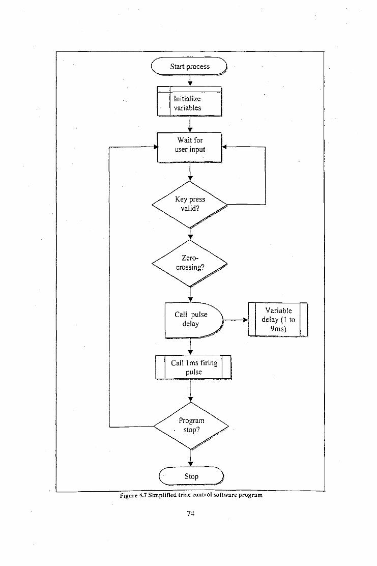
Initializevariables
Wait foruser input
Key pressvalid?
T
Zerocrossing?
Call pulsedelay
Call 1ms firingpulse
T
Programstop?
Variabledelay (I to
9ms)
c T
Stop )Figure 4.7 Simplified triac control software program
74

~N
;;8"
•ry
~~,
Neutral I ~
~
-~
TX
11
~'6J
IR LAMP
500mA
C1O.1uF
R6100R
-L
T
Q16T137
F1
r , ~~
l80R
R7
; I
RS
, R'10k
SI I
R1'OOk R11
(10k
MOC3020
U,
l
""0
I..sjz. ~
R6
330R
R'
I"""" ".", """,," " "."..~""."' ".""".""""" " '''''''iOO'o',o';',To, "".'1'.0',0,""····,,""",, ,,",,···· "".".." """""".",,,,, ,,,,,, ,,,,,,,,.,,.,,.,, ,,,,,,,,,, " """I
i~
~
v' U3B
~S. 5 6
""~ 74126 .
"B!8•ry
:l.~~o
".'~e"§g J1 IS
t~,::g 1" -'--,~ -r-'::J~ 4-fJo ;;" ,r...:.
5~l'olt power supply
IB!>-
U5LM7BOS
3 I VoD
i5
'"-'-
-'-0
vf 1-I
c,_ 2200,F
""0
<;;V1
...... BRIDGE
q. ...
-L-'-0
Figure 4.8 Circuit diagram of the triac power controller
75

• After a key press the program waits for a zero-crossing signal to be detected, this
ensures the firing angle is referenced to zero, and also diminishes EMl and RFI
affects.
• The interrupt service routine is activated and vectors to the software routine, that
in turn selects the firing angle that corresponds to the key press preset value.
• This pulse is delivered through an input/output (1/0) port 4 of the
microcontroller.
A 5-volt power supply is generated from the 240V line voltage through V I, a bridge
rectifier, a filter capacitor (C2) and a voltage regulator (LM7805). The 5-volts voltage
source is used by all the low voltage components including the microcontroller.
4.1.2.5 Evaluation of the triac power control circuit
When the triac power controller is used to drive light loads i.e. less than lA, it functions
remarkably well. An initial test of the circuit functionality had it operating as a light
dimmer, driving a 60W incandescent light bulb. The circuit performed well, such that
when then the firing angle was varied from a small angle to a larger angle, the light bulb
responded by glowing brightly initially to dimming to a dull glow. This load test proved
that the circuit elements functioned properly and that the circuit design worked.
After the initial testing the circuit was subjected to its rated load i.e. an infrared
radiation heater rated at 800W. The circuit failed to switch this rated load successfully.
The circuit element responsible for failure was the power triac. The power triac was
upgraded twice with respective higher current ratings of 15A and 20A, but still the
circuit failed. The reasons for the failure of the circuit was credited to:
• Although the current ratings of the triac far exceeded the load rating (nominal
current of 4A), this value represented an absolute maximum, which in reality
was far less. The inrush current on cold start the destroyed the triac. Inrush
currents of up to IOOA are possible, which would render the triac powerless.
76

• Subsequently it was realised that the triac is a low power-switching device, this
made it unsuitable for the type of loads it needed to control.
• That even when switching the low power incandescent lamp, large voltage
spikes were present that degraded the quality of the line voltage by introducing
noise disturbances.
Due to these reasons a new method of power control was sought that could successfully
handle the rated loads. The effort spent on redesigning and refining the circuit would be
better spent on implementing a more rugged power control option. Although the triac is
still used in many applications and widely published in literature, for the purposes of
this investigation itproved not to meet expectations. (A listing of the software program
in C code used for the triac circuit is provided in Appendix 4).
77

4.1.3 The Insulated Gate Bipolar Transistor Power Controller
The insulated gate bipolar transistor (IGBT) provides a fairly new means of power
control and has found a niche in applications that faH in between that of a bipolar
transistor (BJT) and the power MOSFET. lGBT's are poised to quickly becoming the
preferred means of power control in applications similar to that of the triac and SCR.
These applications include automotive, lighting, home appliances and power
management uses. The IGBT developed in the early 1980's, combines the simplicity of
drive and the excellent fast switching capability of the MOSFET structure with the
ability to handle high current values typical of a bipolar device. These devices can be
programmed to start on the zero crossing and switch off at some later stage, this
technique is known as reverse phase controL Whereas noisy circuits are the product of
triac control because of its turn on, switching off controls an lGBT. This eliminates
noise, in-rush current and EMl effects. With no instantaneous power change to contend
with the controller needs no choke.
The typical voltage output waveforms generated through the use of an IGBT are
presented in figure 4.9 An IGBT can be controlled so as to gradually switch the device
off, resulting in a smoothed load power waveform. This drastically reduces
500 IGBT Chopped waveform
jv 400
300
10U
100 10 100
~100
200
300
400
500
Figure 4.9 IGBT smoothed output voltage waveform
78

any harmonics produced and noise levels on the mains line are diminished or eliminated
ensuring quieter control. The harmonics produced by both the thyristors and IGBT type
controllers are given below. Figure 4.10 shows the resultant harmonics produced by
triac control. Figure 4.1 1 clearly indicates the reductions of harmonics produced that are
evident with the use of IGBT's. Figure 4.14 shows the circuit diagram of the power
controller incorporating an IGBT. This circuit was designed around the IRG4PH30KO
IGBT, which is rated at 20 amps maximum collector current. The design uses a three-
, 3 ~ { a ,1 13 15
Figure 4.10 Typical harmonic spectrum for a triac controller
Figure 4.11 Typical harmonic spectrum for'1 reverse-phase IGBT controller
phase line voltage that is isolated from the rest of the circuit by means of an isolation
transformer as shown in figure 4.12. This ac voltage is rectified using stud rectifiers
(ON I) and filtered through a 2200uF capacitor (C6) as shown in figure 4.13. The circuit
is used as a light dimmer to gauge its performance and its ability to control the power of
a load.
79

Figure 4.12 Three-phase isolation transformer
Figure 4.13 Three-phase voltage rectifier and filter capacitor
80

lP'IR Lamp
D540DV
"~; "I I.
"0u U2§ U, IR210G, TLP251, Rl C 2
HIN la3~~ I lIN HO
, 330R • CaM,. ,.~ 1 VB
.' VCC, ,; VS
~,Dl
5Vl R2C' C2 4k71 J:: ::L sR'
3.3u(l10uF I I' ~riuF I C5 4k7
200nFD2
'J 5V1
-~D6
D7
R5O,1R
c,2200uF:
DN,
T1
I1 ~IIE••.1
3-phasa transformer
;;
~"
"E~
"~
"••~.'""t"
'"lSVdc powersupply
VO
U3,_M7f11S
oij
"
~o
VI
~o
C7330uF
DN'BRIDGE
~
70 I
'iIC !Figure 4.14 Cireuit diagram of the IGBT power controller
81

4.1.3.1 The circuit operation
Using the keypad attached to the 80C515 micro-controller, the user selects the required
power level of the load. The software algorithm then deciphers the key press and
determines the required pulse-width modulated waveform (PWM) to generate. The
program flowchart for the software algorithm is given in figure 4.15 below and its
operation is briefly described as follows:
• The user selects the required power output for the load
• The program determines the suitable PWM waveform based on the percentage
power output
• The point of the zero crossing of the line voltage is detected
• And the PWM waveform generated is sent from an I/O port to the circuit
hardware.
With reference to'figure 4.14 the hardware consists of an IGBT opto-isolator, TLP 251
(U I) that isolates the 80C515 microcontroller from the high voltage circuit components.
Its isolation voltage is rated to 2500Vrms. The PWM enters at pin 2 of UI, which is the
anode of an integrated LED and leaves at pin 6. The PWM then enters pin 3 of the
[GBT driver, IRl I06 (U2) and on exiting on pin 5 is magnified from a 5V peak PWM
waveform to the 15V PWM waveform required by the IGBT. The IGBT (Q I) acts as a
dc voltage switch that drives and controls the voltage across the load, LP I.
Short circuit protection is provided by R5 (O.IQ) this feature eliminates the need for a
fuse, which would otherwise be a heat source in the circuit. The dv/dl can be
drastically slowed down at IGBT turn-off by using a high value gate resistor. R3
(IOOkQ). The typical waveforms for an IGBT at turn-on and at turn-off are depicted in
figures 4.16 and 4.17. The IGBT is protected from ove.r-voltage by a transil diode, 05
rated to a voltage of 400V. A series zener diode, 04 (I5V) is needed to prevent a dead
short circuit occurring across the IGBT in case of the failure of 04. The voltage
regulator, LM7815 (U3), provides the I5V supply that is needed by the le's U I and U2.
82

( Start process)
Initialisevariables
User selectsrequired power
T
User inputvalid?
Zerocrossing?
Pulse width(PWM) waveform
generated
PWM sent fromport 1
(
Programstop?
Stop )Figure 4.15 Simplified IGBT control sofh'i~re program
83

LoAo
.~~J.~!t.l~,.1+~-+-t--+---+-l--- -- 1--- --- -ff --- --- --- ----1---
I \ I . f\n,...~;:l=:=J=::;::::jL,. r~
"-II
--- h. --- -- 1-- --- --- --- -- ---I.... ........._.~,.• -~""1f--lo-4--~-l
Figure 4.t6 Typical waveforms during lGBT turn-on
Anti parallel diodes, D6 and D7, offer further protection to the load and IGBT
respectively in the case of parasitic line inductances. The diodes D I, D2 and D3
eliminate any line disturbances from adversely affecting the circuit. The capacitors C 1
5 act as line voltage filters, reducing the voltage disturbances caused by the switching of
load voltages that could cause erroneous operation of the circuit elements.
.--- ---- .---- ----- ---- ----- .---- ---- -- .. -----
!
I---- ----- -----tJ- ---- __:'S '~---~_
Figure 4.11 Typical waveforms during IGBT turn-off
84

4.1.3.2 Evaluation of the low cost IGBT power controller
In a low power load application, i.e. two incandescent light bulbs in series, the circuit
performs well. The power to the load is controlled successfully such that the dc voltage
in the load is decreased and increased, which is visibly noticed. However when the
controller is used to drive a heavier load, e.g. 800W it failed. Evaluation of the reasons
stem from a combination of the following reasons:
• That although the nominal current rating of the IGBT is well with acceptable
limits for the load under test, the surge current rating falls far below the inrush
current generated with the IR heater.
• The IGBT anticparallel diode, 07, failed to protect the lGBT from line
inductances.
• More effective line voltage filtering to reduce or eliminate the generation of the
voltage spikes was needed.
Coupled with the reasons listed above, some additional information is warranted. That
the IGBT is a new product on the market makes the unit prices fairly costly in
comparison to a triac. This makes the design phase of a controller of this nature an
expensive undertaking, due to component testing, failures and replacement. The IGBT
is a DC voltage switch that does not directly control an ac load it operates in the dc side
of a rectifier. This circuit configuration also succumbs to failure due to the common
grounds of the ac and dc voltage sides.
In the final evaluation of this lGBT controller it is deemed unsuitable for the type of
load under control and again a better method of power control was sought. (A Iisting of
the software program in C code used for the IGBT circuit is provided in Appendix 5).
85

4.1.4 Solid-state switch with PWM cycle control
The two methods of power control presented above proved in practise to fall short of
expectations envisaged for the type of load being controlled. Another method
considered involved the use of an opto-isolated solid-state switch (SSS). The SSS has
two integrated back-to-back SeR's as its control elements. It operates as a zero-voltage
switch, which means it turns on and turns off at a zero crossing. The type of SSS used in
this paper shown in figure 4.18 is the 240D10 manufactured by Opto 22.
Figure 4.18 240DIO solid-state switch
Some the features of this SSS model include the following:
• 4000V optical isolation of input to output
• Nominal current rating of lOA
• Peak surge current rating of 11 OA
• Peak repetitive voltage maximum of 600V
• Zero voltage turn on
• Turn on time: Yz cycle maximum
• Turn off time: y, cycle maximum
• Integrated snubber circuit
86

A SSS is a popular alternative to its mechanical counterpart, the mechanical relay or
contactor. These components suffer from drawbacks that include more frequent
component replacement, poor control ability due to its slow cycle times, dirty contacts
degrade its performance and the heater life may be shortened due to thermal shock
(Evalds, 2002). The electronic configuration of a SSS as depicted in figure 4.\9
comprises a LED on the input, which serves to electrically isolate the high voltage side
~~~flb ~ .,.J
I1
~ i, •- Inpul + nput ""d lo'd
figure 4.191nternal structure of a solid-state switch
from the low voltage microcontroller circuit. This feature of isolation is always of great
importance when high and low voltages are present in the same circuit, as the case in
voltage switching circuits. Over voltage protection of electronic components
necessitates isolation because a low voltage, typically 5V is usually used to drive much
higher voltages, such as 240Vrms. The two back-to-back SeR's control both cycles of
the ac line voltage when triggered by a pulse-width modulated waveform.
The simplified block diagram of the SSS power controller is given in figure 4.20. The
operation of the circuit is straightforward and can be described as follows:
• Using the keypad an IR heater temperature is chosen.
• The micro controller software program determines the appropriate pulse width
of a PWM waveform.
• The generated train of pulses is used to drive the input of the SSS.
•
87

Micro- Solid-State LoadKeypad • controller Relay - . (Infrared
(80C515) (240010) Heater)- -
Figure 4.20 Solid-state power controller configuration
• With reference to the line voltage zero crossing, the power delivered to the IR
heater is varied accordingly.
• The resultant temperature of the IR heater is measured with an infrared sensor
(IR thermometer), the operation of which is discussed in section 4.3.
Figure 4.21 depicts the zero voltage switching capability of the SSS. The SSS always
switches in whole or half cycles of the line voltage, thereby avoiding the occurrence of
EMI and RFI generation. Table 4.2 presents a power control selection chart giving a
range of loads or heaters and their suitable control methods (Evalds, 2002).
/oSO<:I Tu-'!:t C~:iC~t2Tu.~!-Cr:
it lilc ....,:.i.
\ oSCf<._2 ':'"UF'l(;:t
SCn_l :~c~or: !ir:l ./c-:s
Figure 4.21 The zero voltage switching of the solid-state switch
88

Table 4.2 Power control selection chart
Heaterlload Heaterlload
characteristicsControl type Typical applications
type
Constant Onloff, zero-
resistant Slow response voltage Large tllnk heating
elements switched
Medinm-waveThermoforming,
Zero-voltage textiles, industrialinfrared Faster response
switched furnaces and fast waterceramic
heat
Medium-wave Fastest precise Phase-angle
infrared quartz firedPaper and pulp drying
response
Silicon-carbide Load changes in Phase-angle
heaters resistance with age firedHigh temperature ovens
Short-wave Phase-angle
infraredHigh in-rush
fired with softHigh speed paper and
currents ink dryerselements start
4.1.4.1 Evaluation of the SSS power controller
This configuration performed well and out of the three methods investigated for power
control, emerged as a clear favourite. This is due to many factors. some of which
include the following:
• The rugged design of the SSS unit lends itself to the control large loads and is
easily capable of handling the type of load in question.
• The circuit configuration is simple and straightforward when compared to the
other methods studied.
89

• In reference to table 4.2 (EvaIds, 2002), zero-voltage switching is the preferred
method of control for the type of load under study, namely a medium-wave
infrared ceramic heater.
Additional factors that make this type of control the preferred method is the low cost of
the unit compared to the other components studied and also the almost non-exister.O:
disturbances in the line voltages that dominated the other types of control studied.
Figure 4.22 provides a pictorial representation of how the solid-state switch controls the
amount of cycles of the ac mains voltage. Using a pulse-width modulated waveform
(PWM) the percentage power delivered to a load is varied. (The diagram serves only as
a guide and does not demonstrate actual measurements). (The software program in C
code for the SSS power control is incorporated into the software listings of Appendices
2 and 3)
~l- 4()')(_O_po_w_e_rt_O_!O_ad f\Jr\Oi'Cl 500/0 power to load f\J~ 600/0 power to load f\J~ 70'Yopowerto!oad f\J
~1------f\J
~L-_~
Figure 4.22 The cycle control method using the solid-state switch
90

4.2 Infrared Radiation Heater
Electric infrared radiation heaters are typically manufactured to pass electric current
through a heating element made of an alloy of nickel and chromium called nichrome.
The heating element is usually sheathed in either a quartz glass case or encased in a
ceramic material. The type of IR heater studied for this paper is the latter, the ceramic
encased type. It should be noted that many other types of heating elements are available
on the market, e.g. tungsten.
The type of IR heater used in an industrial installation is usually dependant on the
application involved. The four most common types of heaters and their suited
applications are summarised below (Salamander, 1999):
• Quartz tubes are suited for instant on, instant off applications, where heat
sensitive materials are exposed for prolonged periods to a heat source.
• Quartz lamps are also instant on and off type and have a high watt density, best
for high-speed processors.
• Metal-sheath elements used for convection heating needs (e.g. ovens) and are
rugged, cost effective and efficient.
• Ceramic elements are characterised by their gentle heat and are suited for
applications needing an oven and where heating zones are required.
Infrared heaters are available in broadly three categories; long wave, medium wave and
short wave. The type of infrared heater used in this study was the super high
temperature ceramic radiator (SHTS) manufactured by Elstein and has a maximum
operating temperature of 900°C. In addition it has the following specifications:
• Rated power SOOW at 230V
• Radiation efficiency more than 75%
• Heat-up constant approximately 1.2 minutes (63% maximum value)
• Area power densities up to SOkW/m2
91

4.3 Temperature Sensor
Temperature measurement is accomplished through various methods and fall into
mainly four types. These include the following:
o Thermocouples: these are the most widely used types of sensors in the industrial
manufacturing environments. They function by producing a voltage from the
temperature gradient that develops at the junction of two dissimilar metals.
o Resistance temperature detectors (RTD's): operate on the principle that the
resistance to the flow of electricity changes with temperature. RTD's are more
stable and accurate than thermocouples, but cannot be used to measure
extremely high temperatures.
o Thermistors: also change resistance with changing temperatures, but are more
sensitive than thermocouples or RTD's. They are however highly non-linear and
limited to measuring temperatures of a few hundred degrees Celsius.
o Infrared (non-contact) devices are the preferred method of measurement when
the other types are not feasible. They are used in conditions when the above
contact type methods prove troublesome such as monitoring moving objects, in
environments with safety hazards present, where contamination of the target is
likely and when the distance to the target is considerably far.
Infrared sensors also called radiation detectors produce an output signal that correspond
to the amount of infrared radiation that strikes the detector. IR detectors are classified as
either thermal or photon-type detectors. Thermal infrared detectors convert incoming
radiation into heat thereby raising the temperature of the detector. This change in
temperature is then converted into an electrical signal and processed. Broadly defined
there are three types of thermal detectors that include:
o Bolometer, the resistance varies with received radiation.
o Pyroelectric, surface charge varies in response to received radiation.
• Thermopile, consists of multiple thermocouples in series whose voltage output
varies with received radiation
92

Photon-type detectors respond to photons being emitted by an object. The infrared
radiation causes changes in the electrical properties of the photon detector. These
changes can then be monitored as an output signal. There are two main types of photon
infrared detectors (Yoder, 2000):
• Photoconductive: exhibit increased conductivity with received radiation.
• Photovoltaic: convert received radiation into electrical current.
Infrared detectors are further subdivided into various products available for commercial,
industrial and processing use. The existing types fall into four categories:
• Infrared thermocouples: there outputs emulate a thermocouple output and used
in situations where temperatures swings are limited.
• Infrared thermometers: detect infrared energy emitted by objects above
absolute zero. A basic design uses a lens to focus infrared radiation onto an
infrared detector. Ambient temperature variations need to be compensated for in
order to ensure accuracy of measurements.
• Infrared line scanners: produce a thermal map of the surface of a product
moving along a line, mainly used in steel rolling and glass fiber production.
• Infrared thermal imagers: produce a two-dimensional image of a complete
scene being heated and useful for detecting hot spots and triggering alarms.
The type of infrared sensor employed in this paper is a Thermalert Cl sensor avai lable
from Raytek (Raytek C13B). Its specifications include:
• Output linear voltage: IOmVfC
• Optical resolution of4: I at 90% energy
• Spectral response range from 7-18!lm
• Detecting element via thermopile
• Repeatability of±I% of reading
• Temperature resolution of < O.5°C
• Emissivity fixed at 0.95
93

• Response time of 350 ms
• Temperature range: ooe to 5000 e
4.3.1 Installation considerations
When installing the infrared sensor in a particular application there are some important
aspects that need careful planning. The adherence to some simple practices will ensure
that the measurements obtained are accurate and reliable (Ackland, 1998).
First establish the target size i.e. the area to be measured, should fill the instruments
field of view. Suppliers usually recommend that the target size exceed the field of view
by 50%. Because infrared sensors detect radiation from all sources i.e. from energy
transmitted, reflected and emitted by and object. The sensor has to accurately isolate the
emitted radiation for this is the indication of its temperature. If the field of view is larger
than the target size, the background will affect the temperature reading, as shown In
figure 4.23 below.
Another consideration is the determination of the optical resolution and is defined by
IncorrectGood
., '"\', \I \ .II I\ ,\ ,~. ,
Best
...,I \, \I II Ic~1
\
/ /7~-
Sensor
Target greater Target equal Targe-t smalle-r Bat:kgroundthan spot size to spot size than spot size
Figure 4.23 Estimation of the proper target size to an application
94
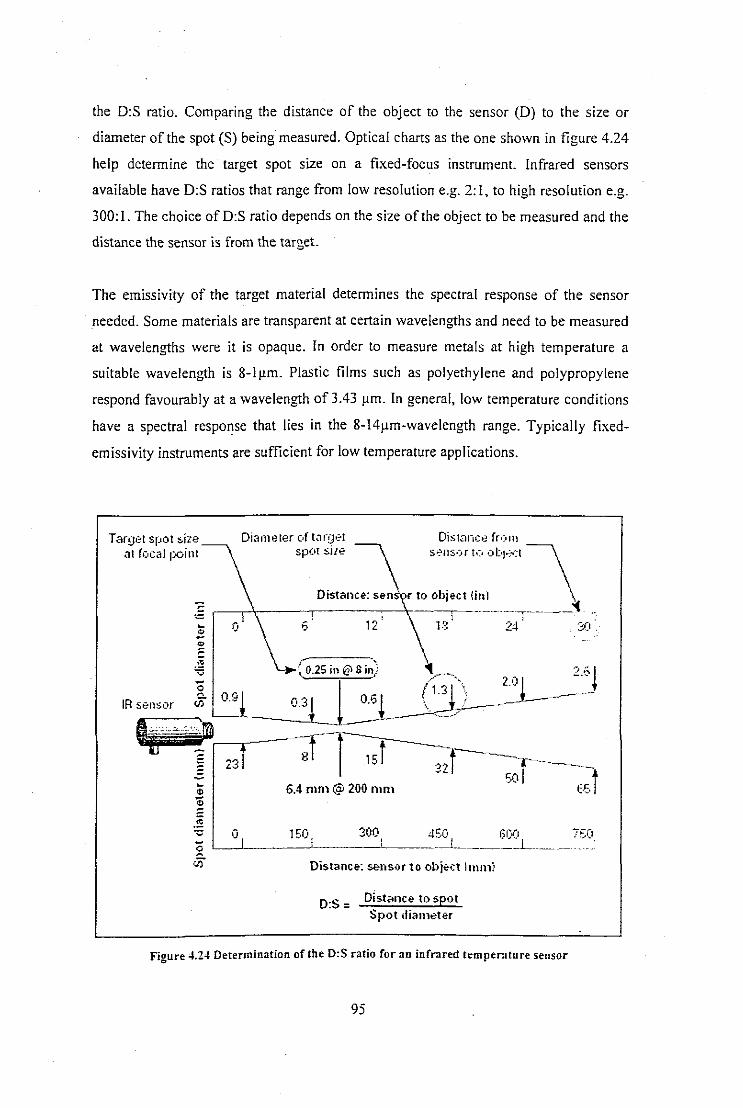
the D:S ratio. Comparing the distance of the object to the senSor (D) to the size or
diameter ofthe spot (S) being measured. Optical charts as the one shown in figure 4.24
help determine the target spot size on a fixed-focus instrument. Infrared sensors
available have D:S ratios that range from low resolution e.g. 2: I, to high resolution e.g.
300:1. The choice ofD:S ratio depends on the size of the object to be measured and the
distance the sensor is from the target.
The emissivity of the target material determines the spectral response of the sensor
needed. Some materials are transparent at certain wavelengths and need to be measured
at wavelengths were it is opaque. In order to measure metals at high temperature a
suitable wavelength is 8-1 Ilm. Plastic films such as polyethylene and polypropylene
respond favourably at a wavelength of 3.43 Ilm. In general, low temperature conditions
have a spectral response that lies in the 8-14Ilm-wavelength range. Typically fixed
emissivity instruments are sufficient for low temperature applications.
7S0
Distance-: sen
Distance: sensor to obje1:t IUHl1i
150
Diameter c'( t.1rO I;-1spot sjzo?
3001 4S01
6CV'----'- -'-__--' ~ L
~IR Sellsor Uf 0.9
Target spot sizeat (()cal point
D:S= Distance to spotSpot djam~ter
Figure 4.24 Determination of the D:S ratio for 3n infrared temperature sensor
95

4.4 Data Acquisition
The data acquisition for temperature measurement instituted III this paper is
accomplished in two ways. In the first instance it is needed to complete the experiment
in which the transfer function of an IR heater is found. Because the software used to
complete the experiment was LabVIEW, a compatible hardware unit the DAQPad-1200
was chosen to facilitate the measurement procedure. In the development of the
controller however the software used was the high level language, C, this precipitated
the use of the on-board analog-to-digital converter. Both these methods when
implemented proved very successfu I.
4.4.1 National Instruments DAQPad-1200
The temperature sensor is interfaced to the data acquisition hardware, the National
Instruments DAQPad-1200. This hardware is a Iow-cost high performance DAQ unit
that communicates with a computer through the parallel port on IBM PCIAT/XT and
compatibles. The features of this unit are the following:
• Eight analog input channels, configured as eight single ended or four differential
inputs.
• 12-bit successive-approximation ADC
• Two 12-bit DAC's with voltage outputs
• 24 lines ofTIL-compatible digital UO
• Three 16-bit counterltimers for timing I/O
• Conversion time (including acquisition time) of 8.5flm
The DAQPad- I200 is also completely software configurable and self-calibrated. The
unit works with two different parallel port types, the Centronics port for printers and the
Enhanced Parallel Port (EP?).
The unit is programmed and operates with LabVIE W software and can brietly be
described as follows:
96

• The DAQPad-1200 on-board AID samples the input sensor temperature. The
integrated conversion performed by the sensor, IOmVrc, represents a
temperature as a voltage between OV and 5V.
• These samples are time stamped and graphed and stored In a text file for
processing at a later stage.
The software program is configured as a data logger to facilitate the transportation of
information to a spreadsheet file. Then using the graphics tool in MsExcel the
information is plotted on a graph, as shown in figures 3.5 to 3.8.
4.4.2 80CSlS Analog-ta-Digital converter
The on-board analog-ta-digital converter (ADC) of the 80C5 I5 has the following
features:
• Eight multiplexed input channels
• Programmable internal reference voltages
• 8-bit resolution within reference voltage range
• 13 machine cycles conversion time (includes sampling time)
• Internal start-of-conversion trigger
• Interrupt request generation after each conversion
The 80C515 method of conversion is via successive approximation using a capacitor
array. The mode in which the ADC is used can be described as follows:
• Single conversion mode
• 2.5V internal reference voltage
The temperature sensor's linear voltage output facilitates interfacing to the on-board
ADC of the microcontroller.
97
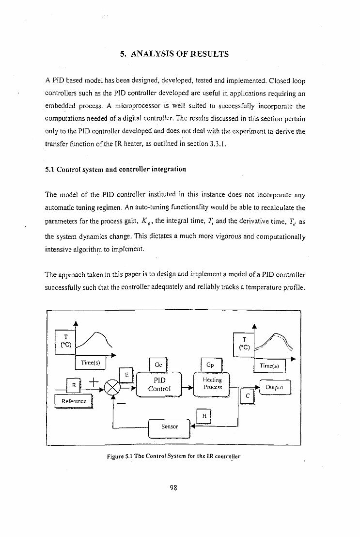
5. ANALYSIS OF RESULTS
A PID based model has been designed, developed, tested and implemented. Closed loop
controllers such as the PlO controller developed are useful in applications requiring an
embedded process. A microprocessor is well suited to successfully incorporate the
computations needed of a digital controller. The results discussed in this section pertain
only to the PlO controller developed and does not deal with the experiment to derive the
transfer function of the lR heater, as outlined in section 3.3.1.
5.1 Control system and controller integration
The model of the PID controller instituted in this instance does not incorporate any
automatic tuning regimen. An auto-tuning functionality would be able to recalculate the
parameters for the process gain, K p' the integral time, T, and the derivative time, Td
as
the system dynamics change. This dictates a much more vigorous and computationally
intensive algorithm to implement.
The approach taken in this paper is to design and implement a model of a PID controller
successfully such that the controller adequately and reliably tracks a temperature profile.
T('C)
T('C)
Time{s)
-8+I Reference I
Sensor
HeatingProcess
Time(s)
'.cJ ,-O_"_lP_"_l.."f
Figure 5.1 The ControJ System for the IR contro!ler
98

Temperature profiles are necessary for the proper processing of many different types of
materials and an example of this is given in figure 1.2. Subjecting the controller to the
control system as illustrated in figure 5.1 and observing how closely the output (C)
follows the input (R) was used as the measure of the success of the controller
implemented.
The mathematical description of the PID controller as given in equation 3.11, needs to
adequately achieve synergy with the mathematical model of the complete control
system as stated in equation 5.1.
C(s)
R(s)
Gc(s)Gp(s)
1+ Gc(s)Gp(s)H(s)(5. I)
As a result the PID controller developed needs to effectively meet the transient and
steady state conditions of the closed loop system. If significant deviations from the set
point occur it could possibly be cause for concern if the product being processed is
temperature sensitive, meaning it has a temperature profile that allows for very little
deviation or offset. This study does not compare the heating profiles for any particular
material against the response of the controller developed. However another approach
was taken, which satisfactorily addresses this issue.
5.2 Comparative testing of the PID controller
In order to g~uge the effectiveness of the PID controller developed, a simpler
proportional type of controller was designed to serve as a basis for comparison. The
an/off regulator does not require the same intense computations as that of the PID
instituted. The on/off algorithm as illustrated in figure 5.2 simply ensures that the set
point temperature is maintained within reasonable limits. The algorithm does not adjust
the pulse-width of the firing pulse when increasing the temperature, as in the case of the
PID algorithm.
A brief explanation of the on/off algorithm is as follows:
99

While loopnot
terminated
Get set point from user
Sample heater temperature
Compute error
Terminate
ISR
y
Samplingdelay
N ~D,-~N_o.:.p_u_ls~e_D
Figure 5.2 Flowchart of the proportional algorithm
100

• After the initialisation of the variables and functions used, the program executes
with the set point as zero, until the user enters a temperature set point above
zero.
• The heater temperature is sampled and an error is generated.
• If the error is positive (> 0), a firing pulse is initiated, however if the error is
less than or equal zero «= 0), no firing pulse is initiated.
• The program waits for the sampling period to complete before taking another
measurement of the heater temperature and repeats the loop.
Laboratory tests have been performed using both the PID and on/off controllers. Each
controller was set to follow a predetermined temperature profile and the results plotted
on MsExcel charts. Figure 5.3 illustrates the laboratory set up for the IR heater and the
Raytek temperature sensor and how they were arranged in order to complete the tests
outlined below. The infrared heater was aligned and fixed to an aluminium
Figure 5.3 laboratory arrangement showing the IR heater and temperature sensor
101

plate. The reason for the aluminium used, was that it possesses a low emissivity and a
high degree of reflectivity. Since the temperature sensor is a function of the emissivity,
only the emissivity from the IR heater then has a bearing on the temperature reading.
5.2.1 Comparative tests at a sampling period of 1 second
Figures 5.4 to 5.6 show the temperature profiles plotted by the two controllers. Table
5.\ indicates an arbitrary desired profile (profile \) programmed into the
microcontroller, the response curves for the on/off and PID models are shown in figure
5.4.
Table 5.1 Temperature set points for profile 1
Temperature setPhase
point ('C)
1 40
2 80
3 150
4 200
6 150
Table 5.2 indicates the desired profile (profile 2) for the on/off and PID models and
their response curves are illustrated in figure 5.5.
Table 5.2 Temperature set points for profile 2
PhaseTemperature set
point ("C)
1 80
2 '100
3 220
4 160
102

r---- --- - -
i ffifffir-~,-•.,--.,.,--.,.,--.. ,'--1f',-f-+-+-+-+-+-+-+-+-+-+-t-+-H
.'J··'1~
.
"'1 J~··II
IJ
i L.r ..- '. ..
,~
,I ,.
I ~
i i
.. , .'...•,
. 'I."",
I
I! ii i I
i I II
I I II
I II I
00000 0 000 0~ V M N ~ 0 m ~ ~ ~..-- ..-- ..-- ..-- .... ..--
00

temperature {0C}
o l2i A '"o 0 ~ g~
'"o ...o '"o
~
CDo 8 ~
o~o
11
21
31
41
51
61
71."
!To" 81=~
"'" 91U.0
101"-0=: 111~
"Co121."
Cl~ 131n i0 3
"0 - <T
""" ~ ~ 1412-;;- So~ : 151n
" 33 "2. 161." '"~ U>~:;;-
1710
"0' 181~
."~
0 191::>;;-N 201
211
221
231
241
251
261
271
281
291
I ~ I I.'
I,
~I
> '.
--4.'
"...
I ~ ~ I I~
. '"", .
!lo.c
41 "".
~
I ~
~
"".
~~~~ .........
I . ••.
.....~I I' ~ .
1 K I,
I I~ I
I. I .
I·.···. . .. ...J ~
----Cl ., ..... f <··e .' .......
-.... >(, .....
J f,
'. f I. ".' IJ.. .,' " ., ..' .' .. . ... t
1 " •.
> .' .. " c.' i' i·~ ·r... '.' '. "..:
, r. '.
I I I
. ".,,' I .. .'.' .. ' .
.. .<: If ". .. , .
L-.. I
I
I
I ..qil
0"0'"
lbll:Od---~:
III

Table 5.3 Comparison of PID and onloff controllers at a sampling period of 1 sec
PID ONIOff
Controller Controller
% Overshoot8% 3%
(lOO'C)
Temperature offset8'C 4'C
(220'C)
Rise time (sec)38 sec 57 sec
(lOO'C to 220'C)
Inspection of the curves in figures 5.4 and 5.5 achieved with a sampling interval of I
second, reveal how the two types of controllers compare. A more concise comparison is
done in table 5.3 with the values obtained through a study of figure 5.5. The factors
considered in this evaluation of the curves are; percentage overshoot, temperature offset
and rise time.
The deduction that is evident from the two controllers with a sampling period of 1
second is that unless rise times are critical and a certain temperature offset is acceptable.
the PID controller is adequate. Otherwise it is a more viable option to use the onloff
controller. Because of the heating dynamics of this type of infrared heater, the warm-up
curve is strongly affected by the long heating time constant.
5.2.2 Comparative tests at a sampling period of lOOms
The PID model produces a significantly better response when the sampling interval is
increased to lOO milliseconds. Figures 5.6 (profile 3) and 5.7 (profile 4) trace the curves
for the PID and on/off models for the new sampling period. Only a restricted portion is
shown here because the buffer used to store the list of temperatures, saturates after 512
samples are received. Nevertheless the portion clearly demonstrates the improved
performance of the PID controller over its on/off counterpart. The curve of figure 5.6
traces a set point from IOOoe to 160°C. The assessment of figure 5.6 as revealed in
105

I L
".'I'I
... ,
.~
•.
~I -~
I~
fiii ". rt.1.
"11~
'!~-;f---l----{---!--,I"~i---I~--+--+--+-_-!---!----f.----ii----rll-+--t-------l----l--·
ii Ii 1-:--+--+--1--1-'1'!I'--+--+---~-+-----lil~I !-:-+--+--+-+~·+-+---l---+---I
lit r i-;__--+--}--I---t----'k-----+--+--t---J':"~ -' f-:--l----{---!--I----il ,-+--+---+---+
;~-+--+--+------;--J--~-,'-----l---+--+--.--J--...-f.-----1-.J, -~~-"
, I

temperature (OC)
I I ! I I I I J[ Ii1
- __ ••• 1
~I'0 I1=0
!U1-.i011U
1
+4 I
-
~F~ II
-
~ ~ N ~ N· N~ m ~ ro ID 0 ~ N Wo 0 0 0 0 0 0 0 0
~ I i I I I I :1
11
jiH~~ I I I i I61 ~- I
~~~ ~ F:Ii: .~ I I ! I
401 I I I I I I I "411
421431
441
451461
471
131 141 _I .1 ']_151'" 1 "R161 ~171 L ~181 ,~ .!
h191 -. h J201 , , .... I
,~f~~~-l I I I
~ 211 .... b-,~ 221 "11 @.!!1 231 S! . h,a 241 ~
~ 251 i.... I,."!2. 261 I .-4:Ji 271 I ..... I
281 "I r I291 ~
301 ~~ I I311 rh I ~_ I I321 ·I----r---~331 I....L341 '. ...... . I-- I
351 "l- I36, I, ;.~1 .,. 11381 rJi391 , , 11.. I
."o'l'"~~
!"...,oa::;
""Q.
:::cn
"a~
o;;~
no3
'""~';;'o
"0'~
'"~o::l;;....
o-.l
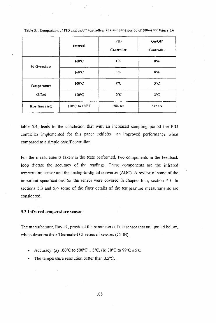
Table 5.4 Comparison of PID and onloff controllers at a sampling period of lOOms for figure 5.6
PID On/OffInterval
Controller Controller
100'C 10/0 0%
°10 Overshoot
160'C 0% 0%
TemperaturelOO'C Z'C 3'C
Offset 160'C O'C rc
Rise time (sec) IDO'C to 160'C 284 sec 312 sec
table 5.4, leads to the conclusion that with an increased sampling period the PID
controller implemented for this paper exhibits an improved performance when
compared to a simple on/off controller.
For the measurements taken· in the tests performed, two components in the feedback
loop dictate the accuracy of the readings. These components are the infrared
temperature sensor and the analog-to-digital converter (ADC). A review of some of the
important specifications for the sensor were covered in chapter four, section 4.3. In
sections 5.3 and 5.4 some of the finer details of the temperature measurements are
considered.
5.3 Infrared temperature sensor
The manufacturer, Raytek, provided the parameters of the sensor that are quoted below,
which describe their Thermalert Cl series of sensors (C I3B).
• Accuracy: (a) 100°C to 500°C ± 3°C, (b) 30°C to 99°C ±6°C
• The temperature resolution better than O.5°c.
108

• The sensor was placed at a distance of 100mm from the lR heater, which forms a
spot size (diameter) of 15mm at the focal point, as indicated by the optical chart
in figure 4.23. This spot diameter proved adequate since the IR heater
dimensions are 41 x 41 mm.
• The sensing head was designed to operate in ambient temperatures from O°C to
70°C. Because the air temperatures at the time of the measurements were in the
region of 25°C to 35°C, the manufacturer's limits were never exceeded.
• The instrument conforms to the following standards of conformity for the
European community:
o EN50081-1: 1992, Electromagnetic emissions
o EN50082-1: 1992, Electromagnetic susceptibility
5.4 Analog-to-digital converter (ADC)
The Siemens 80C515 microcontroller on-board ADC was briefly discussed in chapter
four, section 4.4.2. Some of the more pertinent factors influencing the accuracy of the
ADC measurement are as follows:
• With a 10-bit resolution the ADC can distinguish an incoming voltage into 1024
different levels (210).
• Since the range of the input signal extends from OV to 5V, the least significant
bit (LSB) corresponds to 5.0mV. With a linear output voltage of IOmVrC from
the sensor, a O.5°C resolution of the input signal is possible.
• The sensor is interfaced to the ADC through a single-ended input contiguration.
Although this method is simple to implement, it suffers from a high sensitivity
to noise.
• The 80C515 possesses an internal calibration mechanism and executes two
basic functions, an offset and a linearity calibration. A calibration feature is
useful since the ADC design parameters are adjusted for if a noteworthv drift
occurs. After each reset operation a calibration procedure is automatically
initiated.
109

5.5 Overview of Analysis
Some ofthe more important factors that could influence the temperature readings were
presented. The measurements should therefore be accepted strictly as a trend when
interpreting them. The conclusions however that emerge from the comparative testing of
the two models are clear. The PID controller shows an improved performance at higher
temperatures. The PID model achieves a better rise time, a critical parameter for many
industrial processes, than the on/off regulator. The temperature offset is also greatly
diminished as well as the percentage overshoot, which are all important parameters to
consider when implementing any controller.
110

6. CONCLUSION AND RECOMMENDATIONS
This dissertation is based on theoretical and practical work regarding the design of an
infrared radiation heating profile controller. Both modeling and experimental
techniques have been employed. The focus has been on developing a programmable
and cost-effective controller. This study considered only electric infrared heaters.
A model for a temperature profile controller for an infrared radiation heater has been
proposed. The model is based on a proportional-integral-derivative (PID) control
structure. The PID control design is the oldest and most widely used form of control
in industry. Temperature control is particularly suited to this type of design. Ziegler
Nichols methods have been employed because of their simplicity and effectiveness.
The Ziegler-Nichols method is another tried and trusted technique used for many
years by control engineers. The controller developed though only a simplified first
order model with lag, proved very effective for the purposes of temperature profiling.
The results obtained from comparative tests performed revealed the high efficiency of
the PID model relative to an on/off controller. The tests using a sampling period of
lOOms, although they only covered a restricted temperature range, exposed the
improved performance of the PID design over its on/off counterpart. Although
extensive tests have not been conducted on the controller for the purposes of this
study, the PID model showed promising results. Elaborate testing and verification of
the results are left as a suggestion for any further work and study.
6.1 Problems solved in the dissertation
The problem that this dissertation was required solve was the theoretical design and
hardware implementation of an infrared radiation heating profile controller. This
problem was further divided into many sub-problems, which include the following:
• Conduct an experiment to determine the mathematical model (transfer
function) of an infrared radiation heater.
III

• Design and implement the hardware set-up for the experiment described
above.
• Develop the software program that would allow the accurate display of the
heating and cooling curves of the IR heater under test.
• Investigate the various types of control models available (P, PI and PID) that
would be suitable for type of temperature control required for this study.
• Investigate a hardware platform that proves suitable for the power control
requirements of an IR heater.
• Develop a simpler type of control model, a proportional controller against
which the developed PID control algorithm could be subjected to corn parative
testing.
6.1.1 Experimentally determine the mathematical model of an IR heater.
In order to obtain an accurate mathematical expression of the IR heater used in this
research, a step response test of the IR heater was completed. This method of testing
was done in accordance with the Ziegler-Nichols method, a popular and simple way
of achieving the required results. These results were plotted in a graphical format and
the curves were analysed. Simulation of the obtained transfer function, using Matlab
software, showed good agreement with the practical results. Although the transfer
function represented a first-order model with transport lag, the simulated results
reflected an acceptable accuracy.
6.1.2 Investigate a hardware platform for the power control of an IR heater.
Various methods of power control of the IR heater were investigated and tested. Some
of these methods included:
• Phase angle control using a triac
• Fast switching with an IGBT
• Cycle control with a solid-state switch
The method that proved most successful was the cycle control with a solid-state
switch. The hardware model incorporated this power control design in the final
112

controller circuit. The other types of power control proved problematic for a host of
reasons and some of these include:
• They introduced power line disturbances into the controller circuitry.
• Electromagnetic interference (EMI) as well as radio frequency interference
(RFl) was introduced.
• The type of control method selected proved unsuitable for the type of load
being controlled.
• The power control components (triac and IGBT) failed or were damaged when
used to control the rated load.
The problems listed above all contribute to making the load and the control circuit
unstable and therefore are unsuitable as a method of control.
6.1.3 Investigate the various types of temperature control models available.
The type of temperature control algorithm implemented for this research was the PID
type control. This type of control method is common for the purposes required in the
temperature control problem of this study. In order to gauge accurately the
effectiveness of the controller developed, a simpler type of controller, a proportional
controller, was developed. The PID controller was subjected to comparative testing.
The results confirm the superiority of the PID control model as opposed to the P type
control structure.
6.2 Applications of the results
The results obtained in this research provide the following applications:
• A method of temperature control ofan IR heater;
• And serves as a basis for more intensive IR study.
6.3 Recommendations for further study
I 13

The recommendations on the conclusion of this study acknowledges that IR processing,
whether it be heating or drying, is still a modest researched area. Much work remains to
be done concerning the investigation of the effects of infrared radiation on various
materials. With the use of the controller developed in this paper the study of IR and its
effects on many materials are now possible. A summary of the potential applications
and improvements of the controller are presented below:
• A further comparative study using an auto-tuning PID controller, that
automatically recalculates the parameters of the process as the load demand
changes, is a consideration.
• The enlargement of the buffer used to store the list of temperatures for plotting
needs to be increased so as to provide a clearer picture of the complete
temperature profile.
• Subject the controller to tests on some industrial processes such as the reflow
soldering technique as described in section 1.4.1 and observe the response. A
measure of results is a good indicator of the efficiency of the controller.
• Increase the heating capacity of the infrared heaters i.e. increase the power
densities of the heaters, by mounting an arrangement of heaters on a panel.
This is a more useful and practical way to study the effect on industrial
processes.
• Also conduct experiments to determine the spectral radiation densities of
different heaters and various heater arrangements.
The research conducted for this dissertation serves as a basis for more intensive study
of the many aspects of infrared processing. With an amplified heating capacity that an
arrangement of many infrared heaters offers, a more worthwhile exploratitJn of IR
heating is possible. A modification of the power electronics components in this study
would make this controller a more functionally competent unit for industrial purposes.
6.4 Publications in connection with dissertation
114

1. Adonis, M and Khan, MTE.: 2001. "Infrared Heating Profile Controller"
Proceedings of the 3rd International Conference on Control Theory and
Applications, Pretoria, South Africa, pp.445-449
2. Adonis, M and Khan, MTE.: 2003. Hardware development of an infrared
heating profile controller. Journal of Engineering. Design and Technology.
115
7. REFERENCES
Ackland, K.1une.I998.Selecting the right infrared temperature sensor. Temperature.InTech.
Afzal, T.M; Abe, T. 1999: Some fundamental attributes of far infrared radiationdrying of potato. Drying Technology, VoU7, No.I-2, pp. 137-155.
Altera, I 999.Technical Note: Reflow Soldering Guidelines for Surface-MountDevices. Application note 8J,January J999,ver.3.
Anonymous. 1993.Powder Coat.: better system = improved results. Modern Metals,Vo1.49, pp.76-80.
Anonymous. J994.Perfect finishes with infrared. Metallurgia, VoI.61,pp.7-8.
Anonymous. J996a.Infrared heating systems offer dry/cure advantages.AdhesivesAge,Vo1.39, pp.30-31,
Anonymous.1996b.Electricity, seen through a glass brightly.Process Engineering,Vol.77, pp.21,
Anonymous.I997.Environmental marketplace - Catalytic Infrared heating.Environmental Manager, Vo1.8, pp.15.
Anonymous.l998.Explosive Cooking.Discover, VoU 9, pp.32.
Anonymous.Sep.1999.The Salamander News. Vol. 7, No. 9
Blanc, D.1999.Convective and radiant (IR) curing of bulk and waterborne epoxycoatings as thin layers.Polvmer Engineering and Science,Vo1.39, pp.2487-2497.
Blanc, D; Vessot, S; Laurent, P; Gerard, 1.F.; Andrieu, 1.1997: Study and modelingof coated car painting film by infrared or convective drying. Drying Technologv, Vol.15, No. 9, pp. 2303-2323.
Blanc, D; Laurent, P; Andrieu, J; Gerard, 1.F. 1997: Convective and Radiant (IR)Curing of Bulk and Waterborne Epoxy Coatings as thin layers. Part 1: Methodology.Polvrner Engineering and Science, Vol. 37, No. 12, pp. 1959-1969.
Botero, U.1997.Infrared radiation effects on some functional characteristics of wheatflour. Masters thesis (M.Sc.). University of Manitoba (Canada). Masters AbstractsInternational, VoL36, pp438.
Broadbent, A.D.l998.Comparisonof thermal fixation of reactive dyes on cotton usinginfrared radiation or hot air-American Chemical Societv, Vo1.37, pp.1781-1785.
116
Broadbent, A.D; Cote, B; Fecteau, T; Khatibi-Sarabi, P; Therien, N. 1994: Pre-dryingtextile fabrics with infrared radiation. Textile Research Journal, Vol, 64, No. 3, pp.123-129.
<;:engel, Y.A. 1997. Introduction to thermodynamics and heat transfer. U.S.A; McGraw-Hill.
Chen, Y.S.1995.Infrared heating and welding of thermoplastics and composites ..Thesis(PH.D.)Ohio State University.Dissertation Abstracts International, Vol. 56,pp5148.
ControlIR.Technical brochure: ControlIR-930/935-D-01-B available at:http://www.researchinc.com/tsdlProductslControIIRlcontrolir.htm
Cox,NR;McGee,DE.1989.Use of high density lR for the rapid heating of metals.Industrial Heating, pp46-48.
Dhib, R.1999.Model-based multivariable control of the drying ofa thin sheet of fibresin a continuous infrared dryer.Canadian Journal Of Chemical Engineering, Vol.77,pp.IOSS-1064.
Dhib, R; Broadbent, A.D; Therien, N. 1994: Modelling and simulation of the dryingofthin sheets in a continuous infrared dryer. The Canadian Journal of ChemicalEngineering, Vol. 72, pp. 894-905.
Dhib, R; Therien, N; Broadbent, A.D. 1998: Derivation of a control orientated Ioworder model of the dynamics of an infrared oven for the continuous drying ofa thinsheet of material. The Canadian Journal of Chemical Engineering, Vol. 76, pp. 290299.
Dow, S.1984.Use of radiant infrared in soldering surface mounted devices to printedcircuit boards. Solid State Technology, Vol,27, pp.191-195.
Evalds,P.October.2002.SCR Power Controls Provide Reliable Industrial ElectricHeating. Industrial Heating-The International Journal of Thermal Technology, Vol.LXIX, No. 10.
Fasina, 0.0; Tyler, R.T; Pickard, M.D. 1998: Modelling the infrared radiation heatingof agricultural crops. Drying Technologv, Vol. 16, No. 9-10, pp. 2065-2082.
Foster,A.1996.1nfrared can take the heat.The Engineer, pp22.
Gefran.1999.Technical Brochure: Solid State power Units. power under control.Oct.
Hashimoto, A; Kameoka, T. 1998: Effect of infrared radiation on dryingcharacteristics of wet porous materials. Drying'98 - Proceedings of the 11 th
International Drying Symposium, pp.1891-1898.
HeikkiUi, P. 1993: A study on the drying process of pigment coated paper webs. PhDThesis. Report 92-125-A. Department of Chemical Engineering. Abo Akademi.
117

Heraeus.1992.Technical Brochure: The Golden Figure Eight. 8 convincing argumentsin favour of a unique principle of infrared heat technology. May.
Hottel, RC. 1954. Radiant-Heat Transmission, in W.H McAdams ed., HeatTransmission. 3cd ed. USA; Mc-Graw-Hill.
Hottel, RC; Sarofim, A.F.1996.Radiant heat transfer. Mark's standard handbook formechanical engineers, 10th ed.U.S.A; McGraw-Hill.
Howard, P.1996.End-use Electrotechnologies.Energy Engineering,voI.93,pp.51-65.
Incropera, F.P; DeWitt, D.P.l996. Introduction to heat transfer. 3'd ed. U.S.A. JohnWiley and sons.
1R2000.1998.Technical Brochure:Elstein infrared-system for economical radiationheat.Oct.Elstein.
Katsuhiko, O. 1990. Modem control engineering. ?nd ed. U.S.A; Prentice-Hall.
Knights, M.1997a.Thermoformers give glowing reviews to halogen heatlamps.Plastics Technology, Vo1.43, pp.16.
Knights, M.1997b.Tumbling clamshell oven puts new spin on rotomolding.Plastics Technology, Vol. 43, pp. 35.
Lampinen, M.J; Ojala, K.T; Koski, E. 1991. Modelling and measurements of infrareddryers for coated paper. Drving Technology. Vol. 9, No. 4, pp. 973-1017.
Lavitt,M.1996.lnfrared deicing technique called ready for operational use. AviationWeek And Space Technology, Vo1.l45, pp.104-105.
Leigh, JR. 1988. Temperature measurement and control. United Kingdom; PeterPeregrinus.
Le Person, S; Puiggali, J.R; Baron, M; Roques, M. 1998: Near infrared drying ofphannaceutical thin films: experimental analysis of internal mass transport. ChemicalEngineering and Processing, Vol. 37, pp. 257-263.
Mohan, N; Underland, T.M; Robbins, W.P.1995. Power electronics: converters.applications and design, 2nd ed.U.S.A.John Wiley and sons.
Myers,J.1984.Halogen lamps used as heaters for thermoforming. Modern Plastics,Vol.70, pp.21.
Navarri, P; Andrieu, J; Gevaudan, A. 1992: Studies on infrared and convective dryingof non-hygroscopic solids. Drving'92 - Proceedings of the 8th International DrvingSvmposium, pp.685-693.
I 18
+

Navarri, A;Andrieu, I. 1993: High intensity infrared drying study. Part 1. Case ofcapillary-porous material. Chemical Engineering and Processing, Vol. 32, pp.31 1318.
Ojala, K.T; Lampinen, MJ. 1995. Modelling measurements and efficiencies ofinfrared dryers for paper drying. Handbook of Industrial Drving, 20d ed, pp. 931-976.
Parouffe, I.M; Dostie, M; Mujamdar, A.S; Poulin, A. 1992: Convective transport ininfrared drying. Drying'92 - Proceedings of the 8th International Drying Svrnposium,pp.695-703.
Pettersson, M; Stenstrom, S. 1998. Absorption of infrared radiation and the radiationtransfer in paper. Part 2: Application to infrared dryers. Journal of Pulp and PaperScience, Vol. 24, No. 11, pp. 356-363
Pettersson, M. 1999. Heat transfer and energy efficiency in infrared paper dryers.Doctral Dissertation. Lund University (Sweden), pp. 39-40.
Rosier, M; Klinke, E; Kunz, G. 1995: Drying of Organic Coatings by InfraredRadiation of Different Wavelengths. Radtech Europe, 7th conference on radiationcuring, Maastricht, pp. 462-468.
Sandu, C. 1986: Infrared radiative drying in food engineering: a process analysis.Biotechnologv Progress, Vol. 2, No. 3, pp. 109-119.
Schumacher,H.I 996.lnfra-red soldering from the viewpoint of base materialmanufacturer. Circuit World, Vo1.22, pp.4-8.
Silventoien, I; Palosaari, S. 1982: Drying of water-borne coatings. Acta PolvtechnicaScandinavica, pp. 1-22.
Van Denend,T. I998.lnfrared Predrying Yields Significant benefits. AmericanDyestuff Reporter, VoL8, pp.45-46.
Yamazaki, Y; Hashimoto, A; Honda, T; Shimizu, M. 1992: Optical characteristics ofgelatinous materials in infrared radiation drying. Drying'92 - Proceedings of the 8th
International Drying Symposium. pp. 712-721.
Yoder,1 .May.2000.Taking the mystery out of infrared sensors. Control for the ProcessIndustries.
119

· APPENDIX 1
EMITTANCE VALUES OF PARTICULAR MATERIALS
120

Surface Temperature (Celcius) Emittance
MetalsAluminium, polished 170 0.039
Gold, polished 130 0.018Iron, pure polished 93 0.06
Iron, hot rolled 20 0.77Lead, pure polished 37.8 0.05
Nickel, bright 100 0.041Platinum, polished 93 0.05
Platinum, black 93 0.93
Paints
Varnish, dark glossy 37.8 0.89Enamel 20 0.85-0.95
Red lead paint 100 0.93
Miscellaneous
Brick 20 0.93Ice, smooth 0 0.966
Ice, rough crystals 0 0.985Water 37.8 0.96
121

APPENDIX 2
C CODE LISTING OF THE PID CONTROLLER
122

/********************************************************************/
1* THIS PROGRAM READS THE TEMPERATURE ON AN INTERFACED *11* ADC AND SENDS AN ACTUATING SIGNAL WHICH IS DEPENDANT *11* ON THE SIZE OF THE ERROR BETWEEN THE *11* REFERENCE AND MEASURED OUTPUT *1~ ~
1* THIS IS AN IMPLEMENTATION OF A PID LOOP FOR TEMPERATURE *11* CONTROL *1~ ~
1* By: Marco Adonis *1~ ~
/********************************************************************/
1* Header files *1
#include <stdio.h>#incIude <stdIib.h>#incIude <reg5 I5.h>#incIude <math.h>#define y 50000
1* standard I/O .h-file* I1* standard library .h-file*1
I*special function register for SOC515*1
1* freq = 10Hz (T = 100ms)*1
1* Function Prototypes *1
1* Initialize the serial port *11* Analogue to digital routine '1
1* Delay function *11* Monitor current temperature *1
1* PWM waveform generator *1
void serial init(void);int ADC (void);void deIay(void);void dispIay(void);void puIse(void);void PWM_control(void);void keypad(void);
1* Variable declaration *1long u_delta = 0;long r_in = 0;unsigned int x = 0;
/******************************************************************/
1* MAIN FUNCTION *1/******************************************************************/
void main(void){
long error_0 = 0;Iona- error 1 = o·o _ ,
long error_2 = 0;long y_out = 0;long u = 0;long u_old =0;
123

long ul = 0;long u2 = 0;long u3 = 0;long u_old_1 = 0;long u_old_2 = 0;
EXl = I; I'interrupt for keypad'lITI = I;EAL = I;
seriaUnitO; I'initialise serial port'l
/*****************************************************/I' PID loop initialsation 'I/*****************************************************/
y_out = ADCO;y_out = (y_out);error_O = r_in - y_out;
y_out=ADCO;y_out = (Lout);error_O = r_in - y_out;
I' sample output'l
I'compute error'l
I' To compute the previous actuator outputu_old = (28'error_O) - (49'error_I)'1
u_old_1 = (28'error_O);u_old_2 = (49'error_I);u_old = u_old_1 + u_old_2;
1*****************************************************/
I' MAIN PID CONTROL loop 'II************************~****************************I
I'The PID loop computes the actuator output after each sampl ing intervalu = (u_old + (28'error_0) - (49'error_I) + (21 'error_2))'1
while(!Rl){
y out=ADCO;y_out = (Lout);error_O = (r_in - y_out);
u1 = (28'error_0);u2 = (49'error_I);
124

u3 = (21 *error_2);
u = ul + u2 + u3 + u_old;
1* The computation ofthe incremental actuator output *1u delta = (u - uold);- -
u_old=u;error_2 = error_I;error_1 = error_O;
pulseO; .delayO;displayO;
error_O = 0;u_delta = 0;x= 0;}
}
1* Function Declarations *1
I*determine pulse-width*1
I*call fire pulse*1I*sampling delay*1
1************************************:*************/1* SERIAL PORT INITIALISATION *1/**************************************************/
void seriaUnit(void) (
SCON=Ox5A;BD= I;PCON 1= Ox80;}
1* Initialise UART to mode I *11* Generate baudrate internally *11* Set to 9600 baud@12MHz *1
/***************************************************** /
1* ANALOG TO DIGITAL CONVERTER *1/*****************************************************/
int ADC (void){
unsigned short value = 0; 1* Temperature value returned *1
ADCON = OxF2; '* Select channel 2,single conversion mode *fDAPR = Ox80; 1* Direct conversion, 2.5V int refVoltage *1
while (BSY); 1* Wait while converting *1{;}value = ADDAT; 1* Store value *1
125

return (value); 1* Return temperature measurement *1}
/******************************************************/
I' IMPLEMENTING INTERVAL DELAY '1/***************************************************** *1
void delay(void){
unsigned short i;
i =0;while(i<IOOOO)
{i++;}
}
1* Set up loop counters *1
1* Middle loop '1
/*********************************************************/
I' MONITOR THE CURRENT TEMPERATURE '11***************************************************** ***/
void dispIay(void){
unsigned short q,value = 0; 1* Declare variables '1
printf("\n");value = ADCO; I' Get temperature from ADC '1printf("%3d",value); I' Print values ./
foreq=0;q<=26;q++){printf("\b"); }
}
1***************************************************** /
1* Pulse-width modulated waveform determination '1/***************************************************** I
void PWM_control(void){
if(u_delta <= 0)(T210 = 0; I'stop PWM pulses'lET2 =0;TF2 = I;}else if( u_delta >0 && u_delta <= 5000){x = 10000; I'pwm = IOms'l}else if ( u_delta >5000 && u_delta <= 15000){x = 20000; I'pwm = 20ms'/
126

}else if ( u_delta> 15000)x = 30000;}
}
I' temperature profile presets'l
void keypad(void){
P5 && OxOf;
I'pwm = 30ms'l
}
}
if(p5 = I){rjn =80;}else if (P5 = 2){r_in = 170;
else if (P5 = 3){r_in = 160;}else if (P5 = 4){r_in = 200;}else if (P5 = 5){rjn = 220;}else if (P5 = 6){r_in = 0;}
I'temperature 80°C'1
I'temperature 170°C'1
I'temperature I 60°C'I
I'temperature ZOO°C'I
I' temperature 220°C'1
I'temperature O°C*I
CCEN = Ox80;TF2 =0;ETI= I;
void External I (void) interrupt 2 using 0{keypadO;}
void pulse(void){
CCL3 = (65536UL - x);CCH3 = (65536UL - x»> 8;/' Compare value (duty cycle) '1CRCL = (65536UL - y);CRCH = (65536UL - y»> 8; /. Reload value (50ms period)'/TICON = Ox91; /* Select reload mode 0 and ... *1
1* Bit to start/stop timer' II' Enable compare '1I' Clear interrupt request flag '1I' Enable timer 2 overflow interrupt '1
127

}
void Timer2 (void) interrupt 5 using 0{TF2 = 0; f* Clear overflow flag *f}
/** *** ***** *** ******* *** **** **** * END ***** ************ *******/
128

APPENDIX 3
C CODE LISTING FOR ON/OFF CONTROLLER
129

/*****************************************************************//*THIS PROGRAM READS THE TEMPERATURE ON AN INTERFACED *//* ADC AND SENDS AN ACTUATING SIGNAL WHICH IS DEPENDANT *//* ON THE SIZE OF THE ERROR BETWEEN THE REFERENCE AND *//* MEASURED OUTPUT *//* *//* THIS IS AN IMPLEMENTATION OF A PROPORTIONAL *//* CONTROL LOOP FOR TEMPERATURE CONTROL */r ~
/* By: Marco Adonis */r *//* HARDWARE Version *//*****************************************************************/
/* Header files */
#include <stdio.h>#include <stdlib.h>#include <regS IS.h>#define y 50000
/' Function Prototypes */
void serial init(void);int ADC (void);void delay(void);void display(void);void puIse(void);void PWM_control(void);void keypad(void);
/* Variable declaration */
long error = 0;long r_in =0;unsigned int x = 0;
/* standard 110 .h-file*//* standard library .h-file*/
/* special function register for 80CSIS*//*freq = 10Hz (T = 100Ms)*/
/* Initialize the serial port *//* Analogue to digital routine */
/* Delay function *//* Monitor current temperature '/
/* PWM waveform generator */
/**********************************************************/
/* MAIN FUNCTION *//**********************************************************/
void main(void){
long y_out = 0;
EXI = I;m=l;EAL = I;
seriaUnitO;
//interrupt for zero crossing
130
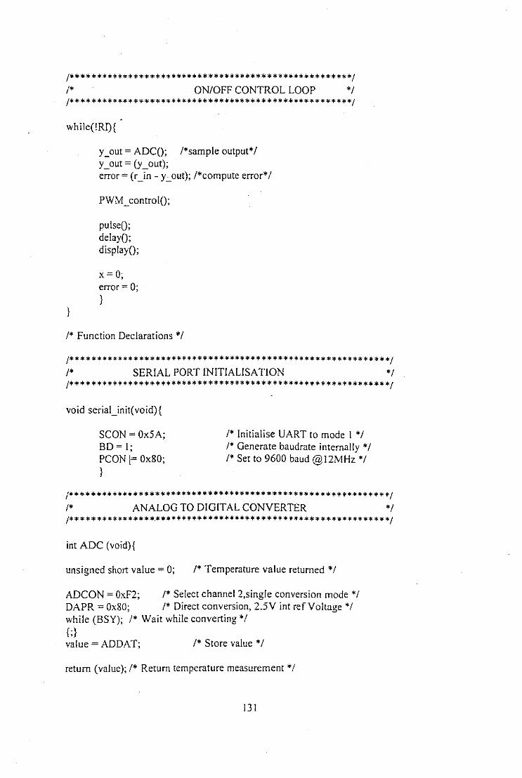
/*****************************************************/
1* ON/OFF CONTROL LOOP *1/*****************************************************/
while(!RI){
y_out = ADCO; I*sample output*1y_out = (y_out);error = (r_in - Ye.out); I*compute error*1
PWM_controIO;
pulseO;delayO;displayO;
x=O;error = 0;}
}
1* Function Declarations *1
/************************************************************/
1* SERIAL PORT INITIALISATION *1/************************************************************/
void seriaUnit(void){
SCON= Ox5A;BD= I;PCON 1= Ox80;}
1* Initialise UART to mode I *11* Generate baudrate internally *11* Set to 9600 baud @ I2M Hz *1
/************************************************************/
1* ANALOG TO DIGITAL CONVERTER *1/****************~************************************ *******/
int ADC (void){
unsigned short value = 0; 1* Temperature value returned *1
ADCON = OxF2; 1* Select channel 2,single conversion mode *1DAPR = Ox80; 1* Direct conversion, 2.5V int refVoltage *1while (BSY); 1* Wait while converting *1I;}value = ADDAT; 1* Store value *1
return (value); 1* Return temperature measurement *1
131

}
/***********************************************************/
1* IMPLEMENTING INTERVAL DELAY *fI************************************~**********************/
void delay(void){
unsigned short i;
i=O;while(i<IOOOO){i++;}
}
1* Set up loop counters *f
1* Middle loop *1
/*************************************************************/
1* MONITOR THE CURRENT TEMPERATURE *f/*************************************************************/
void display(void){
unsigned short q,value = 0; 1* Declare variables *f
printf("In");value = ADCO; 1* Get temperature from ADC *1printf("%3d",value); 1* Print values *1for(q=0;q<=26;q++){printf("\b");}
}
/************************************************************/1* Pulse-width modulated waveform determination *fJ***************************************************** ******/
void PWM_control(void){
if (error <= 0) {T2IO = 0; I*put heater 'off*1ET2= 0;TF2=1;}else if (error> O){
x = 10000; 1* put heater 'on'*1}
}
void pulse(void)
I '?~-

1* Enable compare *11* Clear interrupt request flag *11* Enable timer 2 overflow interrupt *1
{CCU = (65536UL - x);CCH3 = (65536UL - x) » 8;1* Compare value (duty cycle) *1CRCL = (65536UL - y);CRCH = (65536UL - y) » 8; 1* Reload value (50ms period) *1TICON = Ox91; 1* Select reload mode 0 and ...*1
1* Bit to start/stop timer *1CCEN= Ox80;TF2 = 0;ETI = 1;
}
1* temperature profile presets*1
void keypad(void){
P5 && OxOf;
if(P5 = I){r_in = 120;}else if (P5 = 2){r_in = 170;}else if (P5 = 3){r_in=160;}else if(P5 = 4){r_in =200;}else if (P5 = 5){r_in = 220;}else if(P5 = 6){r_in = 0;}
}
I*temperature 120°C*1
I"temperature 170°C*1
I*temperature 160°C*1
I*temperature 200°C*1
I*temperature 220°C*1
I*temperature O°C*I
void Externall (void) interrupt 2 using 0{keypadO;}
void Timer2 (void) interrupt 5 using 0{TF2 = 0; 1* Clear overflow flag *1}
J******************** ************ END * ****** **** ***** ******** *** * **/

APPENDIX 4
C CODE LISTING OF TRIAC POWER CONTROL PROGRAM
134

/******************************************************************/1* Program to fire a pulse on zero-crossing of AC line voltage to vary the *11* load power of an lR emitter & thru ADC read the load temp & store results *11* in a log file *11* POWER CONTROL USING A TRIAC *1/*******************************************************************/
#include <stdio.h>#include <stdlib.h>#include <reg515 .h>#include <math.h>
1* Message Statements *1code char menu[J =
"\n********** MENU ************"
"\nPress 'f to select firing angle""\nPress 's' to start the program";code char txtl [] = "\nSelect the firing angle between 0 and I0 milliseconds» ";code char txt20 = "\nMeasurements in progress(Hit Q to exit)\n ";
1* Function prototypes *1void serial init(void);void set_firing_angle(void);void check_angle(void);void pulse_delay(void);void fire_delay(void);void delay(void);void program_start(void);void program_Ioop(void);
1* Variables declaration *1
unsigned short set_fire =0;Ilunsigned short interval = 0;
1* MAIN FUNCTION *1void main(void){char c;EXO= [;ITO = I;EAL=O;
seriaUnitO;
while(l){printf(menu);c = getcharO;switch(c)
II clear all interrupts
[35
1* interrupt serial port *1

(case 'f':
seU'irin/LangleO;break;
case '5':program_startC);llprogram_loopC);break;
default:printf(menu);break;}}}
1* serial port initialisation *1
void seriaUnit(void){
SCON= OX5A;BD= I;PCON 1= OX80;}
1* setting firing angle *1void set_firing_angle(void){
printf(txtI);scanf(" %d", &set_fire);printf("/n Firing angle delay set to %2d ms", set_fire);//interval =9 - set_fire;}
void program_start(void){P4 = I;pulse_delayC);P4=D;}void pulse delay(void){
CRCL = OxI8;CRCH=OXfc;TICON = Dxl I;TF2 = DJ/I;ET2=I;}
II pulse in positive half
1/ Ims pulse delay
136

if(seUire l= oHfire delayO;P4= I;pulse_delayO;P4=O;delayO;fire delayO;P4= I;pulse_delayO;P4=0;}else{P4 = I;pulse_delayO;P4~0;
delayO;P4 = I;pulse_delayO;P4 =0;}}
void pulse_delay(void){
CRCL=OxI8;CRCH =OXfc;1'2CON = Oxll;TF2 = I;E1'2 = I;}
void fire_delay(void){
CRCL = (65536UL - (set_fire" 1000));CRCH = (65536UL - (set_fire" I000))» 8;1'2CON = Oxll;TF2 = I;E1'2 = I;}
void delay(void){
CRCL = (9000 - (set fire"! 000));CRCH = (9000 - (set_fire" I000)) » 8TF2 = I;E1'2 = I;}
II pulse in positive half
II pulse in negative half
II pulse in positive half
II pulse in negative half
II Ims pulse delay
II variable firing pulse delay
II variable interval delayT2CON = Oxll;
137

/******************************************************************/
/* Function Definitions for Interrupt Service Routines follow */
void ExtemalO (void) interrupt 0 using 0{program_startO;}
void Timer2 (void) interrupt 5 using 0{TF2 = 0;}
138

APPENDIX 5
C CODE LISTING OF IGBT POWER CONTROL PROGRAM
139

/******************************************************************/
'* THIS PROGRAM OUTPUTS A CONTINUOUS STRING OF PULSES AT A *''*FREQUENCY of 100Hz *''* (ie. lOrns Period) *''* INTO STARTS THE PULSE PROGRAM *'*1 A TEST PROGRAM FOR IGBT POWER CONTROL *1/*******************************************************************/
#include <stdio.h>#include <stdlib.h>#include <regSIS .h>I/#define x 7497#define y 8330
void pulse(void);void keypad(void);int x = 0;
void rnain(void){EXO = I;ITO = I;EXI = I;ITI = I;EAL = I;
while(I){};}
void keypad(void)(
I'interrupt for zero crossing
I/interrupt for keypad
PS && OxOf;if(PS = 13){T2IO =0;ET2=O;TF2 = I;} 'I keypad press decodingelse if (PS = 3){x = 833;}else if (PS = I){x= 1666;}else if (PS = 2){x= 2499;}else if (PS = 4){x = 3332;
140

}else if (P5 = 5){x=4165;}else if (P5 = 6){x = 4998;}else if (P5 = 8){x=5831;}else if (P5 = 9){x = 6664;}else if (P5 = 10){x= 7497;}pulseO;
}
void pulse(void){
CCL3 = (65536UL - x);CCH3 = (65536UL - x»> 8;110XFF;I* Compare value (50% duty cycle) *1CRCL = (65536UL - y);CRCH = (65536UL - y)>> 8;IIOXfe; 1* Reload value (500Us period)
*11'2CON = Ox91 ;Ill 1;1/1 9;1* Select reload mode 0 *11* Bit to start/stop timer *1CCEN = Ox80;lIA8; 1* Enable compare *1TF2 = 0; 1* Clear interrupt request flag *1ET2 = 1; 1* Enable timer 2 overflow interrupt *1
}
void extemaIO(void) interrupt 0 using 0{pulseO;}
void ExtemalI (void) interrupt 2 using 0{keypadO;}
void Timer2 (void) interrupt 5 using 0{
TF2 =0;1'2ro = 0;pulseO;}
1* Clear overflow flag *1
141