perceived risk and internet banking in business administration
TRANSCRIPT
PERCEIVED RISK AND INTERNET BANKING
by
KELDON J. BAUER, B.A., M.B.A.
A DISSERTATION
IN
BUSINESS ADMINISTRATION
Submitted to the Graduate Faculty of Texas Tech University in
Panial Fulfillment of the Requirements for
the Degree of
DOCTOR OF PHILOSOPHY
Approved

^^^ \ oil
Copyright 2002 Keldon J Bauer
AH Rights Reserved

ACKNOWLEDGMENTS
I would like to thank the members of my dissertation committee, not only for their
input along the way, but for their flexibility. I would like to thank Dr. Scott Hein for always
pushing this project to be better. The final thesis is so improved over the first drafts that
they appear to be completely different documents. I also would like to thank Dr. Peter
WestfaU for the insight he brought to this project. Through short visits to his office, new
analytical tecliniques were tried that shed a great deal of Hght on the subject of this thesis. I
would like to thank Dr. Philip English for sharpening the focus of the research and
encouraging me along the way. And I would like to thank Dr. Terry von Ende for having
the patience to teach me micro-economics in the first place, and then work with me to
understand it better two to three years later.
But my greatest source of strength, encouragement and support came from my
wonderful wife who endured years of stress and solitude while I worked long, frustrating
hours. Thank you, Sonia, for your love and ungrudging flexibility over the past years of
intense study.
u
TABLE OF CONTENTS
ACKNOWLEDGMENTS ii
ABSTRACT v
LIST OF TABLES vii
LIST OF FIGURES ix
CHAPTER
1 INTRODUCTION 1
2 LITERATURE REVIEW 13
2.1 Internet Market Overview 14 2.1.1 Empirical Evidence about the Internet Market 16 2.1.2 Empirical Evidence Regarding Internet Frictions 18
2.2 Internet Banking Overview 21 2.2.1 Price Competition and Elasticity 22 2.2.2 Motivations for Adopting Remote Banking 29
2.3 Professional Literature 33
2.4 Summary of Literature 37
3 THEORETICAL FRAMEWORK 39
3.1 Base Model Under Certainty 41
3.2 Modeling Preferences Under Uncertainty 47
3.3 The Role of Risk Aversion on Adoption Decisions 50
3.4 Theoretical Summary 55
4 DATA AND METHODOLOGY 57
4.1 Variable Description 66 4.1,1 Differing Degrees of Risk Aversion 69
m
4.2 Base Model Development 70
4.3 Functional Forms Test of the Base Model 79
4.4 Multinomial Model 80
4.5 Modeling the Marginal Propensity to Adopt 82
4.6 Allowing Subjective Probability to Vary 87
5 EMPIRICAL RESULTS 92
5.1 Descriptive Statistics 92
5.2 Base Logistic Regression Model Resvilts 107
5.3 Tests of Functional Form 120 5.3.1 Comment on Risk Aversion 125
5.4 Multinomial Model 127
5.4.1 Multinomial Model with Square Variables 135
5.5 Modeling Marginal Propensity to Adopt 144
5.6 Allowing Subjective Probability to Vary 153
6 CONCLUSIONS AND CONTRIBUTIONS 190
6.1 Conclusions 190
6.2 Contributions 196 6.2.1 Practical Contributions 197 6.2.2 Shortcomings and Future Research 200
REFERENCES 201
IV
ABSTRACT
Bankers and consumers are both interested in the potential for Internet banking.
Individuals have been adopting die Internet in large numbers, with more than half of all
American households having some form of Internet access by 2000. Banks too have been
developing their infrastructure to address what they perceive as a growing demand for online
services, with 84% of all accounts offering some form of Internet banking by 1999.
However, the adoption rate has not followed the hype. By 2000, the proportion of
households using Internet banking was less than 10%. This research looks at the critical
factors needed to promote banking adoption from the consumer's perspective. We use a
consumer utiHty maximization framework, and include in the consumption bundle the
possibihty of using conventional, phone-banking and/or Internet banking. Phone-banking
is added because it could be seen as a substitute for Internet banking. Many of the same
services are available on both, and many of die restrictions are the same, i.e., no cash can be
withdrawn from either.
Using the utihty maximization approach, we are able to conclude that adoption
depends on marginal utiHty gain, marginal cost and a risk premium; where risk premium is
the product of subjective probability of adverse outcomes from the technology and the
utility of each adverse outcome. We use logistic regression to explore what factors are
important to consumers adopting Internet banking in general. A conditional logit model is
used to estimate the sensitivity of different decision factors to the marginal propensity of
phone-bank customers adopting Internet banking and vice-versa.

The overall utility maximization model is consistent with our results from these
logistic regressions. The results presented in this research also support the hypothesis that
the subjective probability of security problems experienced by Internet bank customers is
not the same for all customers, and that it depends on their level of education. Varying
subjective probability means that the risk premixim can be affected by exogenous factors, in
this case education. In other words, banks could affect the risk premium of their customers,
thereby affecting adoption rates.
VI
LIST OF TABLES
4.1 - Joint Probability Table 80
5.1 — Internet and Phone Banking Utilization 93
5.2 — Variables Proxying for Utility Construct 96
5.3 - Budget Constraint Variables 98
5.4 - Education Variable 100
5.5 — Familiarity E-Financial Services 103
5.6 — Risk Treated as a Continuous Variable 105
5.7 — Risk as a Quahtative Variable 107
5.8 — Base Logit Estimates 111
5.9 — More Parsimonious Logit Estimates 114
5.10 - Testing Hypotheses 10-12 117
5.11 - Logit Estimates with One Risk Variable 119
5.12 — Logit Estimates Interacting Education and Age 121
5.13 — Logit Estimates for Functional Form 123
5.14 — Correlation Between Proportion of Liquid Account Balances in an
Internet Band and Risk Aversion 126
5.15 - Base Model Statistics of Fit 128
5.16 -Base Model Using Voice Phone-Banking 130
5.17 - Base Model Using Touchtone 132
5.18 - Base Model Any Phone-Banking 134
5.19 - Multinomial Statistics of Fit 136
5.20 - Squared Model using Voice Phone-Banking 139
vii
5.21 - Squared Model Using Touchtone 141
5.22 - Squared Model Using Any Phone-Banking 143
5.23 - Base P(Internet | Phone-Banking) 146
5.24-Base P(Phone-Banking|Internet) 148
5.25 - Squared P(Intemet | Phone-Banking) 150
5.26 - Squared P(Phone-Banking| Internet) 152
5.27 -Variable Subjective Probability 156
5.28 - Statistics of Fit 160
5.29 - Coefficient Estimates (\''oice) 163
5.30 - Coefficient Estimates (Touchtone) 164
5.31 -Coefficient Estimates (Any) 165
5.32 - P([ntemet | Phone-Banking) 166
5.33 - P(Phone-Banking | Internet) 167
5.34 - Squared Model Statistics of Fit 173
5.35 - Squared Coefficient Estimates (Voice) 177
5.36 - Squared Coefficient Estimates (Touchtone) 179
5.37 - Squared Coefficient Estimates (Any) 181
5.38 - Squared P(Internet | Phone-Banking) 183
5.39 - Squared P(Phone-Banking | Internet) 185
vm
LIST OF FIGURES
1.1 — Internet Usage 1
1.2- Bank Internet Infirastructure 5
3.1 - Utility Maximization 47
5.1 - Effect of Age and Risk on Base Logit Model 158
5.2 -Base P(Internet] Voice) 169
5.3 - Base P(Internet | Touchtone) 169
5.4 - Base P(Internet | Any) 170
5.5 -Base P(Voice|Internet) 170
5.6 — Base P(rouchtone | Internet) 171
5.7 -Base P(Any| Internet) 171
5.8 - Squared P(Intemet| Voice) 187
5.9 - Squared P(Internet ] Touchtone) 187
5.10 - Squared P(Intemet| Any) 188
5.11 - Squared P(Voice | Internet) 188
5.12 - Squared P(Touchtone | Internet) 189
5.13 - Squared P(Any | Internet) 189
IX
CHAPTER 1
INTRODUCTION
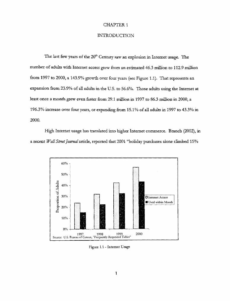
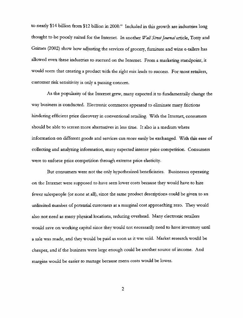
The last few years of the 20* Century saw an explosion in Internet usage. The
number of adults with Internet access grew firom an estimated 46.3 million to 112.9 million
from 1997 to 2000, a 143.9% growth over four years (see Figure 1.1). That represents an
expansion from 23.9% of all adults in the U.S. to 56.6%. Those adults using the Internet at
least once a month grew even faster from 29.1 million in 1997 to 86.3 million in 2000, a
196.3% increase over four years, or expanding from 15.1% of aU adults in 1997 to 43.3% in
2000.
High Internet usage has translated into higher Internet commerce. Branch (2002), in
a recent Wa/I Sireet Journal ntdcle, reported that 2001 "hoUday purchases alone climbed 15%
60% -1
50% -
Ad
ult
s 1
G 30% 0 •ci u O §- 20% -
10% J • 1 1
1997 Source; U.S. Bureau of Census,'
D Internet Access
• U.sed within Month
1998 1999 ^ 2000 Frequendy Requested Tables"
Figure 1.1 - Internet Usage
to nearly $14 bilhon from $12 billion in 2000." Included in this growth are industries long
thought to be poorly sviited for die Internet. In another Wall Street Journal 2irtid&, Totty and
Grimes (2002) show how adjusting the services of grocery, fiamiture and wine e-tailers has
allowed even these industries to succeed on the Internet. From a marketing standpoint, it
would seem that creating a product with the right mix leads to success. For most retailers,
customer risk sensitivity is only a passing concern.
As the popularity of the Internet grew, many expected it to fundamentally change the
way business is conducted. Electronic commerce appeared to eliminate many fiictions
hindering efficient price discovery in conventional retailing. With the Internet, consvimers
should be able to screen more alternatives in less time. It also is a medium where
information on different goods and services can more easily be exchanged. With this ease of
collecting and analyzing information, many expected intense price competition. Consumers
were to enforce price competition through extreme price elasticity.
But consumers were not the only hypothesized beneficiaries. Businesses operating
on the Internet were supposed to have seen lower costs because they would have to hire
fewer salespeople (or none at aU), since the same product descriptions could be given to an
unlimited number of potential customers at a marginal cost approaching zero. They would
also not need as many physical locations, reducing overhead. Many electronic retailers
would save on working capital since they would not necessarily need to have inventory until
a sale was made, and they would be paid as soon as it was sold. Market research would be
cheaper, and if the business were large enough could be another source of income. And
margins would be easier to manage because menu costs would be lower.
Since consumers were expected to cause intense price competition and suppliers
would be able to reduce dieir costs, most of the margin squeeze would, over the long run,
benefit the consumer. The margin squeeze was expected to be enforced by low barriers to
entry (i.e., low start-up costs). Therefore, to compete in the "new economy" businesses
were beginning to believe they had to have an online presence, and most saw theoretical
reasons to believe a margin squeeze was imminent.
Banking traditionally has been very labor intensive. One main hypothetical benefit
to Internet banking adoption has been the reduced cost. Whether giving the customer
information, transferring funds between accounts, or applying for a loan, aU traditional
banking activities include interaction with bank employees, and require a convenient branch
location, paper forms, and a receipt. A transaction as simple as caslnng a check can cost a
bank $1.10\ If customers used the Internet to interact with the bank, the costs would faU
dramatically, even when compared to other forms of remote bank access. Humphreys
(1999) estimates tliat Internet transactions cost less than $0.01 per transaction, compared to
ATM of $0.27, telephone of $0.54, mail of $0.73 and in-person of $1.50. These figures are
almost identical to those quoted by the Department of Commerce^.
But Internet banking supposedly had one other tremendous advantage, pent-up
customer demand. Humphreys (1999) describes demand as follows:
It took nearly 30 years for technology like ATMs to be widely accepted by the public, and screen phone technology never really took off Even the furst attempts at ditect-dial PC home phone banking by some of the larger banks in the middle 1980s met witii Kttle success. Internet banking is
' Robinson, Ten (2000). "Internet banking: Still not a perfect marnage," Informationweek. (782): p. 104, (April 17, 2000).
2 See U.S. Department of Commerce, "The Emerging Digital Economy," Washington D.C., April 1998, p. 29. littp://www.ecotnmcrce.gov/EmcrgingDig,pdf.
different-this is tlie first time customers have led the technology and encouraged banks to move forward rather than the banks pushing the technology on the customer. Consumers want Internet banking because they have the necessary technology-a computer and Internet access-and they are aheady using it to conduct electronic transactions, (p. 8-1)
The implication in this statement is that demand is so high, if you build the
infrastructure, they will come.
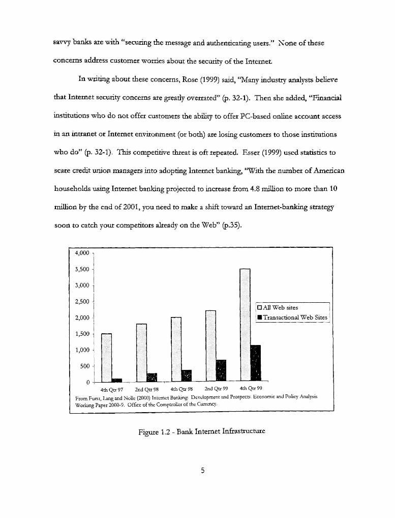
No wonder tiie e-banldng infrastructure has been a major priority at most banks.
Furst, Lang, and Nolle (2000) report that by die thicd quarter of 1999, only 20 percent of
national banks offered Internet banking, which represents 84 percent of all small deposit
accounts. This capabihty was built qiiickly. In the fourth quarter of 1997, only 103 national
banks were reported as offering transactional Internet banking, but by the second quarter of
1998 (six months later), 258 banks were offering Internet banking services (see Figure 1.2).
By the third quarter of 1999, tliis figure had grown to 541. In a study of 3000 banks, MarHn
(2000) reports planned e-banldng investments to grow from $500 million in 2000 to $2.1
biUion in 2005. The ABA Banking Journal estimates that by 2003, 86% of all banks, savings
and loans and credit unions wiU have adopted transactional e-banking technology .
But only 20% of banks had adopted transactional Internet banking in 1999. The
biggest reason for low bank adoption seems to be concerns with security. Their security
concerns are not customer-oriented, but a concern for risk management on the banks' part.
Koonce (1998) quotes libby Ghekiere, chair of NACHA's Internet Council and senior vice
president of electronic commerce with Bank of America's Interactive Banldng Division as
placing traditional banks concerns with "accountability and hability," but those of Internet
^ Bielski, Lauren (2000). Online banking yet to deliver, ABA Bankingjournal, vol. 92 Issue 9
(September), pp. 6,12+.
savvy banks are with "securing the message and audienticating users." None of these
concerns address customer worries about the security of the Internet.
In writing about these concerns, Rose (1999) said, "Many industry analysts beheve
that Internet security concerns are gready overrated" (p. 32-1). Then she added, "Financial
institutions who do not offer customers the ability to offer PC-based online accovmt access
in an intranet or Internet environment (or both) are losing customers to those institutions
who do" (p. 32-1). This competitive threat is oft repeated. Esser (1999) used statistics to
scare credit union managers into adopting Internet banking, "With the number of American
households using Internet banking projected to increase firom 4.8 million to more than 10
miUion by the end of 2001, you need to make a shift toward an Internet-banking strategy
soon to catch yoxir competitors already on the Web" (p.35).
4,000 1
3,500
3,000 -
2,500 J
2,000 \
1,500
1,000
500 -
0 -
From Ft Working
n H 1
OAU Web sites
j • Transactional Web Sites
1 1 4thQtr97 2ndQtr98 4thQtr98 2ndQtr99 4thQtr99
rst, Lting and Nolle (2000) Internet Banking-. Development and Prospects. Economic and Pobcy Analysis
Paper 2000-9. Office of the Comptroller of the Currenq.
Figure 1.2 - Bank Internet Infiastructure
Security concerns in nearly all of die professional literature deal with why banks are
slow to supply Internet banking. Totty (1999) started his article on online security by saying,
"Three years ago, most consumers harbored doubts about online security, especially when it
came to financial transactions or e-commerce. But consumers seem to be getting over their
fears if miUions of online credit card transactions are any indication" (p. 70). He then
insinuated diat customers now place tiieir trust in the due-diiigence of financial institutions
in building secure Internet facilities. But note diat die statistics he quotes are for credit card
transactions. The growth of Internet banking is not as rosy.
By third quarter 1999, 20% of all national banks offered transactional Internet
banking services, according to Furst et al. (2000). Although that may not sound hke many, it
represented 90% of all banking assets and 84% of all small deposit accovints. Despite the
availabihty of Internet banking services, only 5-7% of all households actually used it in 1999.
And although the infrastructure has seen rapid development over the past several years, the
growth in the number of households using e-banking has been almost flat.
Academic research into electronic commerce in general has tested the fricrionless
commerce claims stated earher. Although it appears that prices are lower than at
conventional retailers, as are menu costs, Internet commerce introduces its own fiictions
including what most researchers thus far have called trust. Trust simply means if I order
sometiiing via the Internet, do I get it, in other words, the customers' trust in the firm. But
there is much we still do not know. Research thus far has focused almost exclusively on the
differences between Internet only retailers versus conventional retailer. Due to sales tax
laws, retailers need to choose whether they will offer electronic or conventional services.
Large companies can rarely do both. Few have addressed services offered over the Internet.
Fewer yet have examined electronic financial services. And none have addressed the
demand for Internet services.
Consumer demand for Internet banking services is the main topic of this paper. We
approach demand using a traditional utility optimization framework. In order to compare
our results with other remote banking services, we also examine phone-banking usage using
a similar model. Phone banking was used as a comparison because it allows similar access
(after hours and remote access, without cash access available to ATM users), but enjoys a
much higher adoption rate than that experienced by Internet banking. The model impHes
that consumers configuring access channels to their accounts wiU analyze the expected added
utihty to their account, the expected disutility due to potential security breaches, and any
added cost. Most of the additional cost is computer hardware (in the case of e-banking) or
computer hteracy.
In a static world, rational consumers would assess the marginal benefit of a remote
banking solution with its marginal cost. If the marginal benefit outweighs the marginal cost,
they should adopt it. However, in realitjf, the outcomes are not known in advance.
Therefore, there is an element of risk. Using a subjective set of probabilities for all potential
outcomes, the consumer can assess the expected marginal benefit and compare it to the
expected marginal cost. The difference between the static marginal cost/benefit analysis
under certainty and the dynamic cost/benefit analysis imder uncertainty is called the risk
premium. The theoretical chapter of this research demonstrates that if the risk premium
were eliminated, aU people would adopt all forms of remote banking (or would be indifferent
to adopting it).
Based on the theoretical model, several empirical models are developed to compare
and contrast die Internet banking adoption components mentioned above with those of
phone banking. Fkst, logit models are proposed diat model individual remote banking
decisions over conventional banking. Logit (logistic regression) models estimate die
probabihty of an outcome; we use this technique to estimate the probability of Internet
banking adoption. These models test whether phone banking adoption (or Internet banking
adoption) is a fiinction of the components described in the theoretical model A multiple
dimensional version of this model is then proposed, estimating joint probabihties of
adoption (Internet banking and phone banking).
We consider the outcome space of phone-, Internet and conventional banldng
solutions. If banking consumers are truly rational, they wiU choose the configuration of
conventional, Internet and phone-banking that maximizes expected utility. Philosophically,
consumers would adopt a remote banking solution as long as the expected increase in utility
is larger than the expected cost. The fact that more than two outcomes are possible suggests
that a multinomial empirical approach to this solution would be the most appropriate. Using
this outcome space, we can assess the conditional probability of adopting Internet banking
given the consumer has adopted phone-banking (and vice versa).
This conditional probability wiU help us assess the marginal propensity to adopt
Internet banking given phone-banking (or vice versa). Factors affecting Internet banking
can then be compared with those of phone banking. This comparison will yield information
on what makes phone banking much more widely accepted than Internet banking-greater
benefit, lower cost, less risk, or a combination.

For the consumers' Internet banking risk premium to be interesting to most bankers,
it must be a variable over which they have some influence. Most academic papers assume
that all consumers have identical subjective probability distributions, in essence assuming
that all market participants interpret publicly available information the same way. Identical
subjective probabilities are much easier to model. From a utihty maximization framework,
theories tend to focus on the risk premium assessed by consumers. The risk premium is a
compound construct, made up of both perceived risk and the consumer's risk aversion. To
be consistent with most academic research, we also model the adoption decision by
assvmung identical subjective probability sets.
If we can hypothesize what variables might be important in revising probabihties, we
can model the adoption decision under a varying subjective probability set framework, which
is proposed in this thesis. Most of the variables in the budget constraint (i.e., age, education
and famiHarity with the electronic financial services) are proposed as possible variables
affecting the subjective risk assessment.
This paper adds to the current body of knowledge in several ways. First, the focus
of this paper is on the demand. This is the first research diat empirically models the
consumer adoption of e-banking (or phone banldng for that matter). This is the first paper
that models overall consumption demand for Internet products or services (others have
looked at branding, price elasticity, and other issues, but not overall demand).
Second, this paper examines the role of perceived risk in the Internet commerce
decision. One component in the adoption model is the expected disutihty associated with
adoption. This measure allows us to analyze and hopefully compare the subjective
probability of outcomes leading to disutihty. Because most Internet banking is offered by
banks that also offer conventional banking services, we can model the decision to adopt
Internet banking using variables that measure different components of risk premium.
Initially, we will assume that all consumers have an identical set of subjective probabilities.
Then we will examine what might explain differences in subjective probabihties.
The paper wiU proceed as follows. Chapter 2 reviews academic hterature exploring
the economics of electronic commerce. This review starts with all electronic commerce and
narrows to cover just the electronic banking. Although no pubhshed paper has used
financial economic models to analyze either the characteristics of the demand for Internet
banking or its effect on the bottom-line of the institution, there are relevant papers in related
fields. First, there is a growing hterature focused on the developing e-commerce field.
Second, there are some important financial economic papers exploring the motivation of
banks adopting remote access technologies (focusing on ATMs and phone-banking). Finally,
there is an extensive hterature that examines the financial impact of improved technology in
banking.
The Hterature review also contains a brief review of current articles in the
professional press. Since there is no academic Hterature in the field, the "conventional
wisdom" in die field, among practitioners is also used to develop our understanding theory.
Most of the Hterature in the e-commerce field is either descriptive in its analysis or
broader (considering all industries) in scope than this paper. As such, they tend to miss
important issues relevant to the demand for financial services, such as subjective probabihty.
Most papers analyzing e-commerce are written by management or marketing researchers.
The closest they come to perceived risk is the concept of trust-describing whether one
beheves one wiU receive what one buys over the Internet.
10
Chapter 3 presents the models and the hypotheses impHed by the theory. As
mentioned above, this model is based on the classical optimization of consumer utihty.
Models under certainty and uncertainty are compared to show the impact of risk on the
adoption decision; in short if the outcome were certain, adoption rates of Internet banking
would be significantiy higher. The ultimate outcome of the theoretical model is that
adoption depends on potential utiHty gains by adopting, the consumer's risk premium and
the added cost of the service, including htiman capital cost for computer Hteracy. But the
most interesting outcome is that if Internet banking were offered in an environment of
complete security, all bank customers with the requisite stank costs would use the service.
That finding makes perceived risk the driving force of Internet banking adoption.
Chapter 4 describes the data used as weU as the methodologies proposed to test
those hypotheses. The data used in this paper comes from the Svuvey of Consumer Finance
for 1998 and 1995. This data is compiled by the University of Chicago for the Board of
Governors of the Federal Reserve, and is used more in economics papers than finance
papers. These papers are briefly re^tiewed to determine how the data have been treated in
the past, and the reputation the dataset has in the academic press. The chapter also
proposes several logit models consistent with die theory of Chapter 3 to measure the vaHdity
of the theory and the importance of individual components in the remote banking adoption
decision.
Chapter 5 presents the empkical results of die tests described in Chapter 4. For die
most part, the sections in this chapter correspond widi diose in die mediodology chapter.
The descriptive statistics are presented. Since many of die variables are quahtative, we
present not only firequencies, but critical cross-tabulations. The descriptive statistics section
11

also contains relevant univariate statistical tests. After presenting these descriptive statistics,
the logistic regressions presented in the methodology chapter are presented, supplemented
by follow-up tests to refine the analysis set fordi in Chapter 4.
Chapter 6 synthesizes the findings, tying the theory to the methodology and
empirical findings and interpreting what it all means to the current state of the theory of
electronic commerce in general and the demand for electronic financial services in particular.
It closes by noting the major contributions of this research and the unanswered questions
left by this thesis.
12
CHAPTER 2
LITERATURE REVIEW
There are no papers that look at demand for Internet banking from a micro-
economic perspective. However, diere are odier researchers who have looked at markets for
electronic commerce. Some papers also exist tiiat analyze aspects of the Internet banking
market. There are many claims made by electronic business proponents that the Internet
will significantiy change the retailing landscape, the same can be said in the professional
banking hterature. Some of these claims are based on economic models. Section 2.1
presents these claims as a coherent theory of frictionless economy and reviews academic
papers that describe how well the impHed claims of that theory are supported by empirical
evidence.
A similar coherent "theory" could be developed for Internet banking. Some have
made similar claims, but very Htde research has been done on the subject of Internet
banking, only some theoretical claims and basic empirical evidence. The empirical evidence
includes cost reduction as well as motivations for banks adopting the service. With only one
exception, this Hterature is not aimed at Internet Banking. Some research has been done on
banks' motivation for offering remote access innovations, such as ATMs and phone-
banking. As with the electronic commerce Hterature, these papers focus on the supply of
remote banking services. These papers are briefly summarized in section 2.2 Remote Banking
and compared to the findings of the general electronic commerce Hterature.
Because this research area is so new, die Hterature review is supplemented by a brief
overview of the coverage of Internet banking in the professional press. Unlike the academic
13
press, diere are many articles on this subject in die professional banking journals. Section
2.3 only briefly discusses die current state of conventional wisdom in diis area.
Taken togedier diese areas, electronic commerce and remote banking, form a
foundation upon which die demand for diese services can be analyzed. The findings of
these papers are then summarized in Section 2.4.
2.1 Internet Market Overview"
From a customer perspective, the Internet would be used as a channel for products
and services only if the added utihty outweighed die added cost. Alba et al. (1997) analyzed
the many benefits that interactive home shopping was thought to have over conventional
retailing. OnHne customers have greater alternatives, and can screen them faster and more
efficientiy. In addition, the Internet is a medium through which customers can gain added
information about the good/service. InformaUy using a traditional utiHty maximization
firamework. Alba et al. (1997) talk theoretically about what kinds of goods would seem to
have a competitive advantage online. The analysis uses what the authors consider to be
utiHties versus what they consider costs. None of this analysis considers the subjective
probabihty distribution of possible outcomes, and therefore, does not address the role of
perceived risk of the dehvery system.
Many of the early e-commerce pundits, along with Alba et al. saw the Internet as a
way of overcoming some market frictions. It was assumed that the nature of Internet
shopping would allow customers to search ah sellers and find the products that they wanted
at the cheapest price. Search costs, until now a market friction, would nearly be eliminated
'• Most of the introduction to this section comes from Israilevich (2000).
14

in many industries, which would force the price of goods offered through the Internet closer
to thek margmal costs. It was hoped that the Internet would gready reduce (or eliminate)
much of the frictions involved in the price discovery process.
But consumers were not the only beneficiaries of the new distribution channel,
suppHers would also benefit from the change in business channels. They would be able to
sell products cheaper because they would not have to hire as many salespeople, nor build as
many facihties. As mentioned above, customers would be able to gather information about
products without salespeople. Internet companies could even save on the working capital
needed because they are paid closer to the time when the goods are exchanged, and in some
instances the inventory is not ordered until after a sale is made. In addition, if information is
managed efficiendy, the Internet can save money in marketing research, and customer
information itself may become a profitable by-product of normal business transactions.
Finally, Internet companies are more easily able to manage their margins because the menu
costs are far less than a conventional store.
Unfortunately, there is a downside to the lower operating costs. There are lower
entry costs, lowering the barrier to entry for most industries, worsening the margin squeeze
explained above. This margin squeeze pre-supposes infinite price elasticity, assuming that
price is the only relevant variable to the online shopper.
In short, the Internet was to provide a shopper's Utopia, the ultimate beneficiaries of
the this styHzed model would be the consumers. Normal economic frictions were to
disappear as shoppers, armed with improved information, forced the market to a higher level
of efficiency. Because aU fitrms are seen in this model as operating under perfect
competition, ah benefits of this added efficiency would be captured by the consumer.
15
Section 2.1.1 reviews die tests of most of diese hypotiieses, finding that the styHzed worid
exists primarily on paper. Section 2.1.2 focuses on die frictions tiiat tend to differentiate the
actual Internet market from the theorized Internet market.
2.1.1 Emphical Evidence about the Internet Market
Research has begun to paint a different cyber-landscape than that portrayed by the
Utopian theorists. Brynjolfsson and Smith (2000) tested many of the central hypotheses of
the model described in the previous section, using over 8,500 price observations of
homogeneous books and CDs over a 15-month period. They compared 41 Internet retailers
with conventional retail outiets. The books and CDs chosen were spHt between very
popular items (best-seUers) and more obscure tides (aldiough aU tides had to be held by all
oudets in the study). Prices quoted on the Internet were, on average, 16% lower than in
conventional stores. When adjusting for taxes, shipping and shopping costs the Internet
averaged 9% lower costs, supporting the lowering price hypothesis. Online price
adjustments (a measure of menu costs) were 100 times smaUer than conventional stores,
supporting the lower menu costs hypothesized. Both of those findings support the Utopian
view of the Internet.
However, price dispersion did not necessarily comply with the theory. The raw
price data show that there is more dispersion in Internet prices than among conventional
retailers. The authors re-weight their findings according to market share, and find that
dispersion is now lower among Internet retailers, which raises another problem. The lowest
prices do not have the highest market share, which suggests that consumers are not as price
16
sensitive as die Utopian models would suggest. This is a senous problem for die overall
model, since extreme price elasticity drives much of die findings of die dieorized model.
But diat IS not to say diat price is unimportant to cyber retailers. Price sensitivity
does exist. Goolsbee (2000) tested to see whedier high sales taxes can induce customers to
make more purchases via. die Internet. He used a proprietary survey conducted by Forrester
Research, a market research company m Cambridge, Massachusetts, in December 1997.
They surveyed 110,000 households and asked questions about onhne purchase of 13 types of
goods onhne, as well as consumer demographic data. ControlHng for income, education,
age, and computer access (botii at work and at home), he found that Internet purchases were
higher given high local sales tax rates. These results suggest that there is some price
sensitivity regarding online purchases.
Degeratu, Rangaswamy, and Wu (2000) examined prices of groceries. They
compared sales and price data from sales of 300 subscribers of Peapod, Inc., an online
grocery subscription service, and conventional retailers in the Chicago area between May
1996 and July 1997. The conventional shoppers were interviewed by IRI and consisted of
1,039 shoppers. They found that brand named goods were demanded more by onHne than
conventional customers, but only on certain types of items. They further found that factual
information was more important to online shopper than sensory (appearance) information.
They concluded that evaluating products online could lead to missing information pertinent
to the purchase decision. Wlien there is missing relevant information, customers use the
price as a signal of quahty, and therefore, they do not appear to be as price sensitive as
conventional shoppers.
17
In short, prices seem to be lower for online goods than conventional retail goods,
and menu costs appear to be lower, but Internet consumers do not appear to be as price
sensitive as was hypothesized. The frictionless economy appears to merely be an economy
with different frictions. One of die fictions was identified by Degeratu et al. was that the
information set was different for online shoppers than traditional shoppers.
2.1.2 Empirical E-stidence Regarding Internet Frictions
These conclusions about information were strengthened by Lynch and Ariely (2000)
who investigated price sensitivity in a simulated electronic wine market. They found that as
the cost of information on the quahty of the goods increased, the price sensitivity decreased.
In other words, goods became less price-sensitive as more characteristics are used in the
purchase decision. However, as aU information costs, including price information, become
less expensive, customers become more price-sensitive. Therefore, price-sensitivity can be
used by retailers to their advantage, and if information about a good is withheld from the
market, it may actuahy increase the demand for that good (if its expensive) causing a market
friction.
These general conclusions were supported by demons, Hann, and Hitt (1999), who
found one more friction. They investigated the price competition between ordine travel
agents. They examined tickets written for five corporate cHents for April 1997, and
compared them with other onhne travel agents. Some of thek findings were clearly
damaging to the Utopian cyber-market presented at the beginning of this section. Prices
differed by as much as 18% for the same flight. They found diat some price dispersion is
18
caused by the same company. Bodi the highest and lowest priced onhne travel agents m
thek study were owned by die same parent company. The only difference between the two
agents was that one (die less-expensive) offered a less user-friendly web-design, suggesting
that if shoppers were willing to spend more time, even on the Internet, they could have
gotten better deals on travel in 1997. These findings are consistent with the cost of
mformation argument forwarded by Lynch and Ariely, but would also be consistent with the
hypothesis that the higher the consumer's human capital investment, the more benefit one
gains from Internet shopping.
Another theoretical prediction about the Internet marketplace that does not seem to
be as accurate as it once appeared is that of barriers to entry. Prices of goods on the Internet
were expected to fall close to marginal costs due to the low cost of starting an e-business.
Although it is relatively inexpensive to start an Internet based business, there are economies
to running some types of electronic businesses that may not exist elsewhere. Bakos and
Brynjolfsson (2000) showed that for information based companies on the Internet where
marginal costs are very low, there exists an economy of aggregation, where the company can
simply offer more and more information content to make a more attractive offer. They
show that larger bundlers (usuaUy larger companies) have an advantage in outbidding smaUer
ones. Further, they show that larger bundlers (companies that bundle many information
products together) can make a tougher competitor than smaUer, single-product companies.
They find that in some instances simply adding one information product to thek line, they
can enter and dominate a new market; which is easier to do if you have many such products
that can be added at low marginal costs. Because of the strategic advantages discussed thus
19
far, small information companies may have Httie incentive to create new informational
content (although larger bundlers may have more incentive to iimovate).
Bakos and Brynjolfsson's conclusions only are appHcable to informational goods.
Physical goods with larger marginal costs do not tend to foUow these principles, although
bundling goods and services have long been seen as adding value to the customers. It is
unclear from thek research whether this economy of aggregation holds for financial services,
and would probably depend on the marginal cost of those services. If financial services tend
to have lower marginal costs, thek findings could mean that larger financial companies have
a competitive edge in electronic commerce. As wiU be discussed later, (account) aggregation
is a hot topic in the professional Internet banking Hterature, and has much the same
arguments at it root as informational product aggregation.
The final friction fotind in the empirical work on Internet commerce is typicahy
described as trust, since it is usuaUy covered in the marketing Hterature. Israelevich identifies
it as risk aversion, but as used in the Hterature, it is whoUy insufficient for financial assets.
Trust refers to whether the customer beheves that the product wiU Hve up to promises made
about it. Trust can refer to product quahty, as weh as the retailer's service after the sale (or
whether the goods are ever shipped to the customer). Examples ki the Hterature include
Internet customers brand loyalty in the Shankar Rangaswamy and Pustateri (1999). This
loyalty was further tested with onhne retailers that have been used before. If the customer
had a good experience the first time, they are likely to return.
These conclusions are supported by Brynjolfsson and Smith (2000), who found that
retailers with an estabhshed name and reputation in conventional retailing could command
between 8-9% higher prices than die competition, just because they feh more confident that
20
they would get what they purchased, and that problems could be resolved with a real person
in a convenient location. This is one of very few papers in this genre that
Urban, Sultan, and QuaHs (1999) used a cHnical experiment to examine the effect
that an imbiased onhne "advisor" had on the purchase of products. The "advisors" in
essence provided information about the product or the retailer, and were in no way
associated with the retailer. They found that more subjects were willing to purchase the
product recommended by the unbiased advisor than those without the "trusted" advisor.
Since this was a cHnical experiment, not involving a real company or real money, there had
to have been some halo effect in the results.
2.2 Internet Banking Overview
Many of the expectations of e-commerce were shared by those theorizing the impact
of the Internet on distributing financial services in general and banking in particular through
this new medium. l ike Alba et al., Mols (1998) also saw consumers maxknizing utiHty
subject to budget constraints. He also expected price competition, suggesting that those
banks wanting to participate in this channel wiU have to offer better rates, because Internet
customers are sophisticated and extremely price-conscious. Mol sees a world where banks
focus thek development in eitiier branch banking or Internet banking. This hnpHes that die
overall cost structure will depend on the dominant channel chosen.
The hnpHcation of tins e-banking vision is extreme price elasticity. If the theories of
e-commerce are consistent across channels (from electronic retaihng to electronic financial
services) then we would expect a lower cost strucmre, and higher price elasticity, which
would lead margms to be squeezed to approximately marginal costs. In addition, barriers to
21
entrance wiU be low, enhancing competition and reducing costs to consumers. These are
essentially the same assumptions made of e-commerce in general.
Few empirical papers in this genre look specificaUy at Internet banking. Although
many of these papers look at adoption of technology, some of thek knphcations can be
apphed to e-banking. Section 2.2.1 will review empirical findings regarding price
competition and elasticity. Section 2.2.2 wiU review empirical findings regarding motivations
for adopting remote banking services.
2.2.1 Price Competition and Elasticity
Price competition suggests that the production function of banks participating in
Internet banking wiU shift. In addition the empirical efficiency of the industry, how close
banks appear to be operating to the most efficient expansion path, would deteriorate as long
as aU banks do not adopt these technologies simultaneously. Mol would expect that not aU
will adopt them at aU, so the efficient expansion path would permanendy deteriorate.
Cost efficiency with lower overhead could be interpreted as increased scale
economies. One of die earhest investigations into the effect of technology on the scale
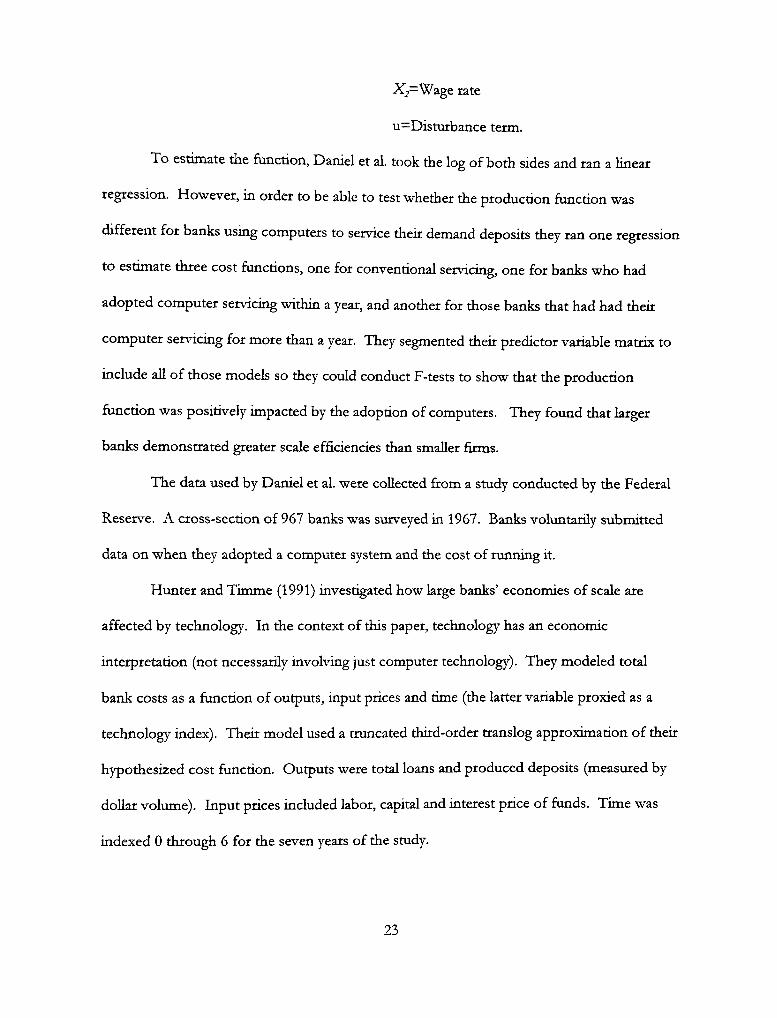
economies of banking was conducted by Daniel, Longbrake, and Murphy (1973). They
looked at differences in scale economies brought about by adoption of computer technology
to service demand deposits. Thek proposed model was rather simple. They assumed the
following Cobb-Douglas production function:
C = p,X,^^X^'e" (2.1)
where X,=Number of demand deposit accounts
22
X^=Wage rate
u=Disturbance term.
To estimate die function, Daniel et al. took die log of bodi sides and ran a Hnear
regression. However, in order to be able to test whether die production fiinction was
different for banks using computers to service thek demand deposits they ran one regression
to estimate three cost functions, one for conventional servicing, one for banks who had
adopted computer servicing widiin a year, and another for those banks that had had thek
computer servicing for more than a year. They segmented thek predictor variable matrix to
include all of those models so they could conduct F-tests to show that the production
function was positively impacted by the adoption of computers. They found that larger
banks demonstrated greater scale efficiencies than smaUer firms.
The data used by Daniel et al. were coUected from a study conducted by the Federal
Reserve. A cross-section of 967 banks was surveyed in 1967. Banks voluntarily submitted
data on when they adopted a computer system and the cost of running it.
Hunter and Tknme (1991) investigated how large banks' economies of scale are
affected by technology. In the context of this paper, technology has an economic
interpretation (not necessarily involving just computer technology). They modeled total
bank costs as a function of outputs, input prices and time (the latter variable proxied as a
technology index). Thek model used a truncated thkd-order translog approximation of thek
hypothesized cost function. Outputs were total loans and produced deposits (measured by
doUar volume). Input prices included labor, capital and interest price of funds. Time was
indexed 0 through 6 for the seven years of the study.
23
Hunter and Timme used data primarily from the year-end caU reports for 1980-86.
They only consider the 400 largest banks, and farther restrict thek sample to banks in states
that aUow branching, as were money center banks. Thek final sample included 219 banks,
which they subdivided kito smaUer (110) and larger banks (109).
They found that technology had increased the efficient bank size by shifting the cost
curve downward and outward. And Hke Daniel et al., they found that larger banks had
benefited more from technological change than smaUer banks. The shift in the cost function
had changed the optimal mix among smaUer institutions.
Another paper germane to the topic of improved cost structure is Hancock,
Humphrey, and Wilcox (1999) who investigated the economies of scale experienced by
consoHdation of Fedwke electronic fimds transfer operations. Previous research had shown
Httie evidence of scale economies, attributing most cost savings to technical advances.
But this investigation used a longer time period, discounted transition costs, and
used indexed input prices. Using a translog function to estimate the production function,
they concluded that there were significant economies of scale realized in the consoHdation,
but fakly Htde teclinical improvement. The biggest reason for the difference in conclusion
was probably the time interval. The shorter time interval was still picking up cost noise due
to the transition.
Domowitz (2001) investigated the relationship between technology implementation
and its effect on trading costs and intermediation in the securities trading hidustry. Using
regression analysis, he found evidence of cost reduction.
In short, the economies of scale Hterature tends to agree that technology improves
the cost structure for banks and other financial services providers and tends to favor larger
24
banks. The larger the bank, the more savings are possible once some of the more routine
tasks are automated. In die context of Internet banking, the adoption of technology has
always reduced bank cost structures. Therefore, it is consistent with evidence from earher
technology adoption that die cost stmcture would improve by adoption of Internet banking.
Much of the recent work in bank cost determinants biulds on the foundation of
production functions developed above. But in addition to estimating the production
function, they examine the dispersion within the production possibihty frontier. If Mols'
(1998) theory of strategic bank channel specialization is correct, banks wUl not adopt
uniformly, creating greater dispersion from the overaU banking efficiency frontier. The
distance from that frontier is a measure of efficiency of individual banks. Taken together,
these efficiency measures can assess the overaU efficiency of the banking industry. The
measure of efficiency depends on which variables are taken into account. The papers
reviewed here are just some of the more recent examples in this genre, and do not represent
an extensive Hst, but these are the most important exploring the role of technology and
confounding variables. The earher papers in this genre agree that there is a large dispersion
in efficiency between banks. In addition, there is an extensive Hst of working papers that
further explore bank efficiency (in some cases thek definitions of efficiency differ gready
from that described here and may not be germane to this topic).
Rogers (1998) examined whether nontraditional activities can explain a portion of
the observed inefficiency. In addition to cost efficiency, he considered revenue and profit
efficiency. Three functions were estimated using translog models. One fiinction was
estimated for cost, another for revenue and yet another for profit using a distribution free
25

approach. The input consisted of panel data on some 2,000 banks over five years. The data
were separated into banks operating in states with limited or statewide branching.
To test whether nontraditional activities affect the efficiency, Rogers separates these
models ushig a restricted-unrestricted model methodology. Then efficiency measures were
calculated for each observation, and mean and standard deviations were estimated. FinaUy,
t-statistics were calculated on the differences between the mean efficiency calculations using
die restricted versus utuestricted models. He found a statisricaUy significant cost efficiency,
and profit efficiency improvement among those with more nontraditional activities. In
short, part of the observed inefficiency is explained by the bank's dependence on non-
traditional activities. Not including these activities in models in earher studies has overstated
the inefficiency in the industry.
WTieelock and Wilson (1999) investigated productivity, efficiency and the role of
technical progress in both productivity and efficiency. They begin by developing a model of
change in efficiency over time. The model is designed to extract the components of the
efficiency change into pure efficiency changes, changes in scale economies and changes in
technology. The underiying concept is that if a bank does nothing over time, it wiU look less
efficient because scale economies, technologies and other forces change the industry
production function over time. If enough banks do nothing while other banks irmovate and
improve thek production technology, the industry wUl look inefficient because a few banks
have become more efficient. This paper attempts to identifjr how much of die kiefficiency
of banks over trnie are due to each of these individual component.
Wheelock and WUson used a data envelopment analysis (DEA) and derived
Mahnquist indices of productivity changes for die components in question. They used data
26

firom die CaU Report for die fkst quarter of each year 1984-93. They made estimates on aU
banks, and just those surviving for the entire time period (with the same quahtative results).
They assumed that the technology used in production was continuous across aU banks.
They conclude that over the time period smdied, banks have experienced large
advances in technology. This improvement is attributed to technological change, which has
moved the production function, coming closer to constant returns to scale. However,
technical efficiency has decHned over time. Wheelock and WUson explain the decline in
technical efficiency as unequal adoption of technology. They argue that a minority of banks
in each size class has been successfuUy implementing technological advancements. One area
of technological innovation cited by these authors is Internet banking. These findings are
consistent with Mols' contention that some banks wiU make a strategic choice not to adopt
Internet banking. If Internet banking is more efficient, then the technical efficiency
deterioration would be explained by the tendency for banks to specialize into Internet
banking institutions versus non-Internet banking institutions.
Furst et al. (2000) are the only researchers who have looked specificaUy at the affect
of adoption of Internet banking to thek cost structure. They test the cost structure of banks
with Internet banking capability versus those without, and find the production function to
be different. But because they do not account for the cost structure before adoption, it is
unclear whether the difference in costs is due to the adoption of Internet banking or
whether Internet bankkig is due to the fact that these banks had lower costs, and could
therefore afford to invest in this new technology.
There are no pubhshed research addressmg price elasticity. Mols (1998) cites one of
his unpubhshed papers to conclude that those customers who use home-banking are "more
27
satisfied with thek bank, have higher intentions of repurchasing, provide more positive
word-of-mouth communication and are less likely to switch to another bank." AU of these
findings suggest higher loyalty, which is counter to Mol's own contention that these
customers are more price-sensitive. A recent article by Schwaiger and Locarek-Junge (1998)
also suggested that electronic banking could be used to retain bank customers.
The research investigating the types of barriers to entry do not have a comparative
empirical echo among finance researchers. It does appear from descriptive data in Furst et
al. (2000) that early adoption of Internet technology has been concentrated among the
largest banks first,^ suggesting that at least originaUy, there may have been a barrier to entry
in this market, probably due in large measure to buUding the necessary security protocols. If
bundling has the same impact on financial assets as described earher by Bakos and
Brynjolfsson (1999), then these larger banks wiU have an advantage, in that they have
developed more financial services offered via the Internet. Mols (1998) would suggest that
smaUer banks might want to focus on branch operations due to thek strategic disadvantage.
In short, there is some sketchy evidence that Internet banking does reduce the cost
structure of banks. Unlike the e-commerce Hterature no researcher has looked at interest
rates offered by banks for onhne products to see if better deals for the customers are
offered. But since the majority of banks offering onhne services are traditional banks, it is
unlikely that the interest rates offered online customers differ from conventional banking
products. This is verj^ different fiom the findmgs of the e-commerce Hterature. It suggests
5 Tliis statement appears to be true also in the U.K. from the findings reported in Jayawardhena and
Foley (2000).
28
diat onhne bank customers are not overly price sensitive, which is what Mol says he found ki
a survey of onhne bank customers.
2.2.2 Motivations for Adopting Remote Banking
The reasons why the styHzed model of electronic commerce does not hold have not
been investigated. In that context, these fiictions are not explained. However one research
topic unique to the finance Hterature is why banks decide to adopt technology, aside from
concerns about lowering costs. This may be a different kind of friction in this market, since
it would affect the overaU technical efficiency of the industry. Mol would suggest that the
decision were made based on whether smaUer banks felt they could compete. Few
researchers have addressed this issue as it relates to Internet banking.
However, Hannan and McDoweU (1984) investigated the economic determinants of
ATM adoption. They found evidence that large banks that were operating in a bank holding
company, and in states where branching was aUowed were more likely to offer ATM
services. Thek conclusions tended to focus on the banks' size and organization. However,
they also controUed for wages and demand deposits, which may reflect something about the
ultimate user of the service. They also found that areas with higher wage rates, and high
levels of demand deposits to total deposits were also more likely to offer ATMs.
Three years later, Hannan and McDoweU (1987) explored the connection between
adoption of ATMs and the previous employment of ATMs by competitors, hypothesizing
that adoption of new technology may foUow a diffusion process. In this study, no economic
data on consumers was used, tiiey only considered individual bank data, finding support for
29
diek hypothesis that there is a relationship between supply structure of the market and bank
adoption of ATMs.
In 1990, Hannan and McDoweU explored the effect of technology adoption on
market structure, as described by concentration. Again the technology adoption tested is
ATM adoption. Although banking firms did use ATM access to attract customers,
concentration did not tend to change drasticaUy because smaU and large banks tended to add
the capabUity at roughly the same time. In short, Hannan and McDoweU contend that
ATMs were used originaUy by large banks to lure away customers fiom other banks. SmaUer
banks then combined into networks to batde these competitive forces to protect thek
current customer base. Although large banks used ATMs to attract customers away from
larger banks, the concentration did not change much, because smaUer banks began offering
the same services.
The reason banks adopted the technology at roughly the same time, regardless of
size may be explained by game theory, which is another approach used to analyze this issue.
Bouckaert and Degryse (1995) studied the phone-banking adoption decision. As in Degryse
(1996), which studied remote banking in general, they apply game theory to bank
management's decision to initiate remote banldng services. These papers model the decision
of adopting remote banking through strategic games, where cost of gaining or maintaining
marketshare is the object.
Matutes and PadUla (1994) used a skmlar approach to explain under what conditions
banks would share an ATM network and when diey would use a stand-alone ATM system.
They pokit out that die customer benefits from a shared network in two-ways. Fkst, a
shared system offers better access to deposits (die network effect) and k forces diek bank to
30
be more competitive in rates offered, because they can not compete on location (the
substitution effect). In investigating the trade-off between the network effect and the
substitution effect, they conclude that only two states wUl obtain a possible equUibrium,
either a subset of banks share thek network (what they caU partial compatibiHty) or aU banks
go it alone (total incompatibihty). In thek model fuU compatibiHty does not ever obtain
unless withdrawal or interchange fees are charged for use of an ATM that is not owned by
your bank. It is not clear whether the model would be observed in the United States. One
reason for partial compatibiHty is that banks in the network can use the network as a weapon
to keep other banks out of thek market.
By contrast, Byers and Lederer (2001) use an operations research approach to
finding the optimal mix of remote banking channels offered by a bank. The configuration
can include branch banking, home PC banking, owned ATMs, ATMs owned by others, or
any combination of these. This paper uses economic modeHng as weU as operations
research to analyze the distribution chaimel configuration from the bank management's
perspective. Marketwide shifts in configuration and avaUabihty of service are modeled and
predicted using sensitivit)' analysis whUe adjusting level of consumer demand for electronic
versus branch access, or the cost structure of electronic banking. They are optimizing profit
to the bank given certain input parameters. One of the more interesting Byers and Lederer's
findings in Hght of the focus of this paper is that changes in consumer behavior and attitudes
have a proformd effect on the distribution strategy. Thek model suggests that pure
electronic banks are only viable when die electronic-preferring segment is nearly twice the
size of the branch-preferring segment. One major drawback to this model is that it treats
31
many issues as static variables. Even the response of the customer to bank offers of Internet
banking is treated as a known, which it clearly is not.
In Mols (2000), the adoption of Danish Internet banking is modeled as dependent
on managers' characteristics. Do managers feel threatened by being replaced? How
comfortable are the managers with computers? Again, survey data were used. He found
that banks where managers did not feel threatened were more likely to adopt this
distribution technology.
The findings of these "marketabUity papers" is that one reason banks choose to
adopt remote banking is to gain customers through offering them a service that thek current
bank does not offer. Another reason for adopting onhne banking is to guard against other
banks stealing your customers. They model why banks adopt new technology, as weU as
why not aU banks adopt the technology. One assumption made in aU of these models is that
the probabihty of consumer adoption is known and constant. But even these have a friction.
Mols showed that this propensity is tempered by how threatened bank managers may feel.
In short, the frictions in the financial services industry appear to be different than
those in general e-commerce. But the participants are also different, since they are usuaUy
conventional financial services firms offering thek cHents one more distribution channel.
One of the biggest "frictions" in this context is why they chose to offer Internet banking at
aU. These films tend to offer Internet banking services because they seek a competitive
advantage, seek to guard agakist incursions on thek customer base, because that mix
maximizes profits, or because managers are in favor of it.
32
2.3 Professional Literature
Much of the professional press has echoed in large measure the findings of the
academic press. Bank Marketing (2001") claims, "purely onhne banks ought to have an
insurmountable advantage over brick-and-mortar institutions." They cite then lower
overhead, higher interest-rates on product offerings, more convenient hours and locations as
these unmatchable advantages. But despite conventional wisdom, a new report from
Meridien Research claims that if consumers can choose between a website with higher
interest-rates on products and a banker with a website and a physical location, the bank with
the physical location wiU win. Only 2% of the increase in onhne banking was captured by
pure online banks, the rest was captured by traditional banks with a web presence.
These findings were recendy reaffirmed by Mearian (2001). Citing a report by
Jupiter Media Metrix, he reports that traffic increased 110.5% fiom July 2000 to July 2001 at
banks with both a physical and cyber branches. Over that same time period traffic at purely
cyber-banks feU 8.1%. Although the onhne only banks seemed to have such tremendous
advantages, for most bank customers, the benefits of a physical location outweigh the
disadvantages in sHghtiy higher interest. The advantages entimerated contain physical access
to money, customer service and perceived longevity. These finding suggest that there are
barriers to entry, and that price sensitivity is not as strong as hypothesized.
But simply starting a transactional cyber-branch does not ensure profits. To profit hi
this market, banks must first "crack tiie code on customer priorities," clahns Slywotzky
(2001). Only then, should a bank digitize. Aldiough he gives European examples of banks
that have successfiiUy implemented an onhne presence, most American financial mstitutions
are on thek own fittkig financial offerings to customer deskes. Key Corp., for kistance.
33
seems to dimk diat most potential cHents do not know how convenient onhne bankkig is.
According to a Bank Marketing (2001'') article, tiie bank is maUmg 118,000 bags of popcorn
to customers widi checkkig accounts and an ATM or debit card, teUkig diem diat ki die time
k takes to pop die com in die bag, tiiey could have estabhshed an onhne account.
For most banks, the strategy to increase onhne banldng is to kicrease consumers'
utiHty with the service. One of die biggest bankkig catch-phrases auned at knproving utiHty
is account aggregation. As described in the academic section of this chapter, aggregation
refers to bringing many related information products together. In banking, it is bringing
together many different financial services. Since the beginning of the onhne banking
movement, banks have seen this as a way of increasing the value to the customer. For banks
that had an in-house investment and/or insurance department, aggregation meant simply
cross-selHng. To those institutions without in-house resources, they would simply bring
together partners to a cyber maU, usuaUy run by a thkd-party vendor. Moss (2001) saw these
a^regator sites as die wave of the future. She predicts that in the future customers wUl be
able to transfer funds, purchase financial products, and obtain financial planning advice.
However, Bruno (2001) clakned that the current aggregation solutions are too
primitive to Hve up to thek expectations. In addition, the pay-off to the financial institutions
is unclear as far as thek abUity to cross-seU products from one financial product to another.
The primary objective of aggregation is to retain current customers and cross-seU products,
and it is nearly impossible to demonstrate how weU it has accompHshed this objective. In
fact, Bruno suggested that current trends ki the industry will make thkd-party aggregators
more responsible for demonstrating the value they are adding, which he thinks is not what
34
tiiey are charging. Over the long mn, he expects any aggregating to be done by a lead
financial institution, cutting out the thkd party vendor.
This reahty check is not restiicted to aggregators. The entire onhne banking service
is beginning to be evaluated as to whether it is worth the current investment Unfortimately,
not everyone is in agreement on the answer. Orr (2001) says that over five years, if a
"typical" bank has 50,000 onhne customers, offering a "fuU plate" of e-banldng services, they
should be able to realize a net present value of $5 per customer, or an IRR of 60%. Of
course, that rosy figure is contradicted by Matthew Lawler, an e-bankuig consultant
interviewed by Kingson (2001), who claims that a bank must achieve an adoption rate of at
least 10-15% of thek customer base before thek onhne banking services are profitable.
Benaroch and Kaufmaim (2000) beheve that the analysis used by both of these "experts" is
inappropriate. They show how an option framework and the Black-Scholes model could be
used to analyze the bank's electronic banking decision.
But aU of these analysts focus the institution's attention on the benefits of the
technology to the bank. Which is why when security risk is discussed, the institution
typicaUy thinks about what the ramifications of these risks are to themselves and thek
shareholders. Many articles discuss security issues, but rarely is the effect on the customer
mentioned other than ki passing. For kistance, even though Schacklett (2000) says, "[Credit
union] members need to know they're protected." But she starts out by saying that half of
Internet shoppers are concerned about security, and half of Americans not yet on Internet
are also concerned with security. With that kind of an introduction, it soimds Hke concern
about security does not affect adoption of Internet banking. The rest of die article does not
refer to die needs of customers at aU.
35
However, Rob Lee, Executive Vice President of ALLTEL RLS, in a speech to die
Mortgage Bankers Association of America (2001) showed die real power of perceived risk of
the Internet. After explainkig that mortgage appHcations can currentiy be made online, with
many of die fields of die appHcation being "pre-populated" widi mformation from the
kistitution's files or the customer's credit report, making the form much easier to complete,
he explained diat few customers are using it. Citing a recent Fannie Mae survey, he says that
56% of recent home buyers used the Internet to get mortgage information, 4% of recent
purchasers apphed onhne, and only 2% completed the entire mortgage onhne. He
continued, "Why are so many people holding back? WeU, Fannie Mae foimd that answer,
too. They're afraid ... afraid to give out so much personal information online. ... Thek
fears are focused on die Internet itself Sixty percent of the people surveyed said the
Internet is not a secure place to conduct personal finances."
And if that source is not enough, even potential customers are Hsting security as a
major issue in deciding whether to go ordine. In a recent Association Management (2001)
article questioning whether electronic banking was right "for you," the three factors most
important to making that decision were Hsted as first - security, second — cost, and thkd -
overaU fit. Note that security, risk of losing resources or information, was Hsted as the first
factor.
In short, the professional press has also assumed that online bankkig would reduce
thek costs, improve thek profit margins and kitensify competition. The realization has been
different from the perceived model. Ahnost aU practitioners have assumed the key to
Internet adoption was improving the benefit to the customer. But there seems to be some
36
evidence tiiat one of die biggest drawbacks firom die consumer's standpoint is die perceived
risk of exchanging personal financial kiformation over die Internet.
2.4 Summary of Literature
The Internet was originaUy seen as creating a world much closer to the fiictionless
world hypodiesized m Utopian economic models. It was seen as a medium tiiat could reduce
information asymmetries among customers durough search engkies and "shop-bots." And
since the information set would be closer to uniform among shoppers, it was assumed that
the Internet would enhance price competition, sknpHfy the price discovery process and that
price elasticity would kicrease. In the case of financial services largely the same expectations
were made.
Empirical evidence shows that although e-taUer costs in this medium are lower, and
economic pressure forces thek prices lower, frictions stiU remain. AU bundles offered by
compaiues and received by consumers are not homogeneous. Each retaUer offers different
levels of service and information along with products. These services include ease of use of
the interface, customer support after the sale, abihty to talk to representatives in person
should things go wrong, and trust engendered in the business and product being offered,
which may explain the observed preference of traditional banks offering Internet banking
over purely onHne banks.
In short, although Internet commerce does reduce some frictions experienced in the
conventional economy, it does not eliminate them, and may have created some of its own.
Businesses are beginning to use those "fiictions" to differentiate thek products and erect
competitive barriers to entry in this developing market for goods and services.
37
Aldiough tills Hterature explains some tilings about the Internet marketplace, nearly
aU of the Internet research considered only those firms that conducted aU of thek buskiess
electronicaUy. The demand for banking services is a different question in most cases.
Traditional banks are offering conventional financial services via an Internet channel. Thek
customers can either choose to kiteract with the bank in person or via the Internet. This
paper explores what factors affect the decision to adopt the Internet chaimel. It adds to the
current Hterature in several ways. Fkst, it explores why customers would choose to interact
with a conventional business via the Internet rather than in person or through estabhshed
mediums. Second, it adds a component of subjective risk of security problems to the micro-
economic optimization. Thkd, using the traditional factors pertinent to solving the classical
consumer problem, we are able to see whether these subjective probabihties of security
problems are significant when deciding to adopt Internet banking as a distribution channel.
The effect of subjective probabihties, perceived risk of security breaches, is also analyzed
over time to see if it changes.
38
CHAPTER 3
THEORETICAL FRAMEWORIC
The analysis of this chapter uses micro-economic theory of consumer utiHty
maximization to assess the choice process for remote access to banking accounts. The maki
object of this paper is to better understand Internet banking adoption. Internet bankkig is
analyzed by itself as weU as in contrast with a close substitute, phone-bankmg. A model is
presented that demonstrates the utiHty maximization choice model for Internet services,
phone-banking and in the more reahstic case of both services.
These two added remote access services have some things in common. They both
extend the hours that busy people can access thek accounts. The services offered, balance
inquiry and transfer, are similar. The touchtone version of phone-banking is computer
based, meaning that those who are computer Hterate are more likely to feel comfortable
enough with the interface to easUy adopt it, much Hke that of Internet banking.
However, they also have important differences. They differ in the amount of
computer investment requked by the customer, and the inherent risks (or at least the risk
perceived by the consumer) in the two different mediums.
This framework is developed so that the importance of different factors of the
models of choice of these two different remote access services can be contrasted. In 1998,
43% of aU households used phone-banking of some kind, whUe only 6% of aU households
participated in Internet banking. Using the model presented in this chapter, the potential
factors critical to Internet adoption can be compared with that of phone-bankmg to
determine what characteristics should be most critical.
39
To analyze how different characteristics affect the decision to adopt remote bank
access services we develop a utiHty maximizing model, and explain the ramifications via the
marginal rate of substitution (MRS) between traditional bank accounts and identical accounts
that aUow for Internet access and/or phone-banking. The MRS can depend on the utiHty
function used to model consumer preferences. There is no clear consensus on the best
utihty function for bank accounts (or cash, since transactions accounts act as a substimte for
cash). Most researchers use either a form of the CES, or the translog function.^
Many utihty functions have been found to be satisfactory for preference modeling.
Bath, Kraft, and Wiest (1977) used an S-Branch UtiHty Tree to model preference behavior
between bank assets. The S-Brainch model was derived from the CES function, and thereby
agrees in general principle with Short and VUlanueva (1977) and Bufman, Leonardo, and
Leiderman (1993), who used CES functions to model preference behavior for savings
deposits/money and currency, respectively.
However, others find the transcendental logarithmic (translog) utiHty fiinction^ to be
a good descriptor of consumer preferences. Ewis and Fisher (1984) showed that demand
for money in the United States could be modeled by the Translog function. The function
was used to model the demand for money ki Choi and Sosin (1992), as weU as demand for
monetary aggregates in Serletis and Robb (1986).
' Other functions have been used as well such as the Cobb-Douglas, Miniflex Laurent and Generalized Leontief, but those listed here seem to be the most widely accepted.
7 See Brown and Heien (1972). 8 This function was developed by Jorgensen and Lau (1975).
40
3.1 Base Model Under Certainty
We develop the model in two steps. The first assumes that the customer is
completely certain about the security of thek bank accounts. In short, this model assumes
that risks do not exist, to examine how consumers should behave in a riskless worid, with
fiiU information about thek abUities to operate with remote banking technologies. Then we
wiU relax the "riskless" assumption, to develop a testable model. To compare the value of
remote banking services in general, we make a simpHfying assumption that consumers can
choose between two otherwise identical accounts at the same bank. The first account,
designated account T, offers an account with only traditional banking services, no remote
banking services. The second account, account R, offers traditional and remote banking
services'. We begin our description of the certainty model by describing the assumptions
that drive it. The major assumptions of the model are hsted below:
Al . Complete Certainty Assumption: No security risks exist for either the traditional accovmt
or the account with remote bank access (Internet and/or Phone-banking). That
means that in this styHzed world, die probabUity of suffering disutihty fiom robbery
is held to be zero. For the conventional accounts diis could be explained by deposk
insurance for most accounts. For remote bank accounts this is only a temporary
assumption. AddirionaUy, we assume diat die consumer has a perfect gauge of diek
own computer/Internet banking abUity and phone-banking abUity, and diat tiaey
tiierefore know how much utiHty tiiey wiU gain by adopting diese technologies.
9 The model presented here is addressing the question of why traditional banks can not get their customers to adopt an additional interface, it does not address why people would adopt an Internet only bank. The model dierefore addresses the largest segment of the current Internet bank market.
41
A2. Substitutability. Accounts T and R offer exacdy die same financial products widi die
same kiterest, restrictions, fees, etc. The only way ki which die two dkfer is tiiat
account R also aUows customers to access diek account remotely via the Internet
and/or phone-bankhig, whereas account T offers no remote access. They would be,
therefore, perfect substitutes, except for tiie differing levels of added utiHty and cost
of the service of the remote account.
A3. Utility Function: The overaU utiHty derived from bankkig accounts can be represented
as:
U{x) = f{x)-^d,h,(x)^d.,h^(x) (3.1)
where x = amount deposited in account.
f(x) = UtiHty function associated with traditional account
(5', = 1 if phone service is used by consumer, 0 otherwise
h^(x) = the added utiHty by phone access to account
<5 = 1 if Internet service is used by consumer, 0 otherwise
^zM ~ th^ added utiHty by Internet access to account
Note that the ptirpose of the < is to add another distribution channel. If the
constxmer uses (or has at least authorized) phone banking, then 5^ is one. If 5^ is
one, then the consumer uses (or has at least authorized) Internet banking. Since
Internet banking is conducted under certainty, at worst, the added utiHty could be
zero, or hf(x) > 0 and h2(x) > 0.
A4. Marginal Utility: As the amount held in accounts increases, the utiHty associated with
both forms of remote access services increases. If the consumer is completely
42
technologicaUy UHterate, they wUl know that; but since there is no security risk, no
disutihty is expected. But for those who even gain smaU amounts of utihty from the
added access, the more money held in accounts, the more utiHty consumers gain
from the abihty to manage them remotely. Because there is some utiHty associated
with these capabiHties, as the amount deposited increases, the opportunity costs of
not having these remote services increases, h^ '(x) > 0 and h2'(x) > 0.
Note that although there is only one type of "traditional" account, in our model
there are three unique remote accounts: Internet and phone-banking, only Internet banking,
and only phone banking. It is also important to note that this utiHty structure impHes by
itself that if aU relevant costs were equal between the two types of accounts that the remote
access account would dominate the traditional bank account, because for aU x's, U would be
greater than if any S were 0.
If the aU relevant costs of the two accounts are not equal, we must first consider the
comparative costs of the different accounts. Since many of the costs, including opportunity
costs, are the same for traditional and remote access accounts, the base cost function (from
the consumer's perspective) should be the same for account T and account R, we wUl now
consider those costs that are different between die two. In addition to the base costs, those
considering an Internet or phone account may be charged an additional fee for access to or
use of these remote facUities. In the case of Internet bankkig, tiiey wUl also have to pay for
access to the Internet, and diey may have to buy a computer. Depending on diek computer
and/or Internet experience, they may have to incur a human capital development cost
(traming costs). This human capital cost may be smaUer with phone banking. To some
43
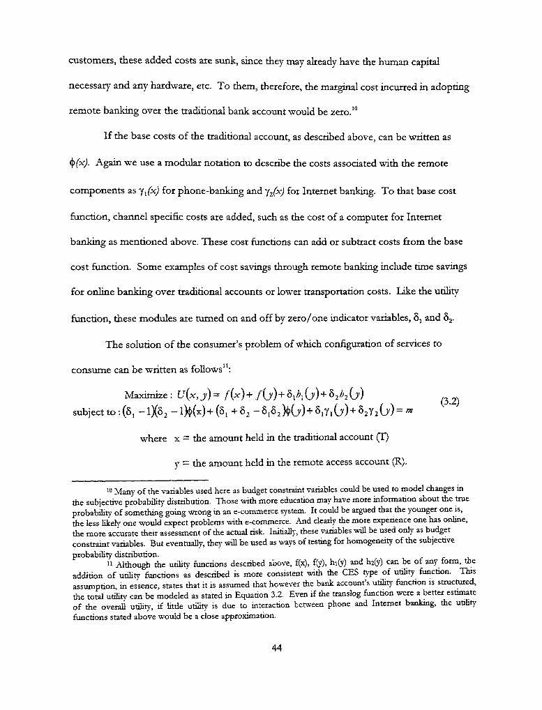
customers, these added costs are sunk, since they may akeady have the human capital
necessary and any hardware, etc. To them, therefore, the marginal cost incurred in adopting
remote banking over the traditional bank account would be zero.'"
If the base costs of the traditional account, as described above, can be written as
^(x). Again we use a modular notation to describe the costs associated with the remote
components as y^fx) for phone-banking and jzfx) for Internet banking. To that base cost
function, channel specific costs are added, such as the cost of a computer for Internet
banking as mentioned above. These cost functions can add or subtract costs from the base
cost fiinction. Some examples of cost savings through remote banking include time savings
for online banking over traditional accounts or lower transportation costs. Like the utiHty
function, these modules are turned on and off by zero/one indicator variables, 5, and 82.
The solution of the consumer's problem of which configuration of services to
consume can be written as foUows :
Maxknize: U{x,j)=f{x)+fij)+b,l>,ij)+b^l>^ij)
subjectto:(5, - 1 X 8 2 - l M x ) + ( 5 , + 5 , - 5 , 5 2 > t ) 0 ' ) + 5,Y,0 ')+52y2G) = ^
where x = the amount held in the traditional account (T)
y = the amount held m the remote access account (R).
1" Many of the variables used here as budget constraint variables could be used to model changes in the subjective probability distribution. Those with more education may have more information about the true probability of something going wrong in an e-commerce system. It could be argued that die younger one is, die less likelv one would expect problems widi e-commerce. And clearly the more experience one has online, the more accurate their assessment of die actual risk. Initially, tiiese variables will be used only as budget constraint variables. But eventually, diey will be used as ways of testing for homogeneity of die subjective probability distribution.
» Aldiough die utility ftinctions described above, f(x), f(y), hi(y) and hiij) can be of any form, die addition of utility fiinctions as described is more consistent widi die CES type of utility function. This assumption, in essence, states diat it is assumed that however die bank account's utility function is strucmred, die total utility can be modeled as stated in Equation 3.2. Even if die translog function were a better estimate of die overaU utility, if Uttie utiUty is due to interaction between phone and Internet banking, die utiHty fiinctions stated above would be a close approximation.
44
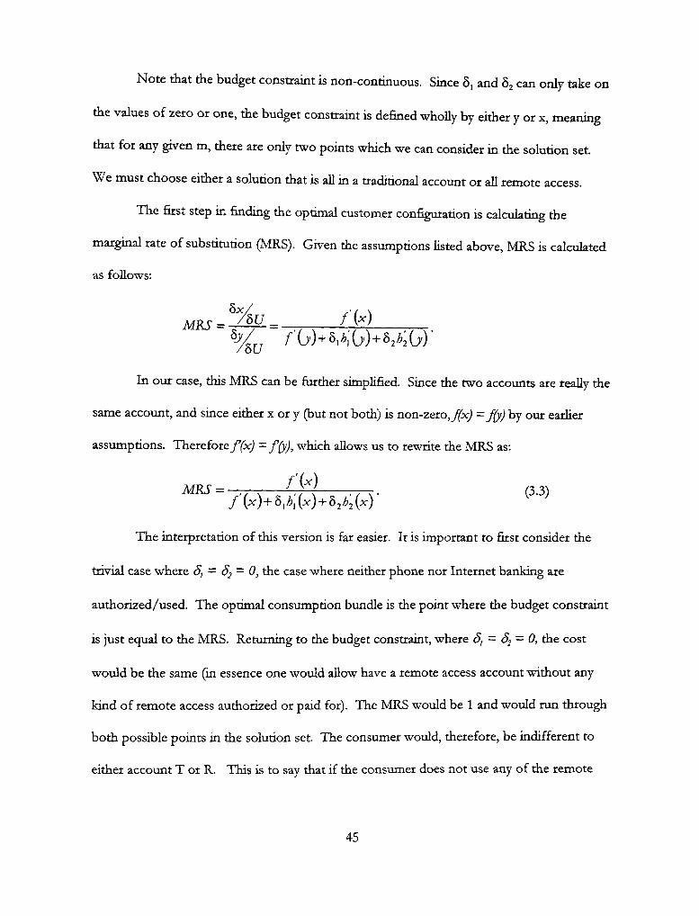
Note tiiat die budget constraint is non-continuous. Skice 6, and 83 can only take on
die values of zero or one, die budget consttahit is defined whoUy by eidier y or x, meamng
diat for any given m, there are only two pokits which we can consider ki the solution set
We must choose eidier a solution diat is aU ki a traditional account or aU remote access.
The fkst step in fhidkig the opthnal customer configuration is calculating the
margmal rate of substitution (MRS). Given tiie assumptions Hsted above, MRS is calculated
as foUows:
^y^^ f'{jh^A{j)+hh2{j)'
In our case, this MRS can be fiirther simpHfied. Since the two accounts are reaUy the
same account, and smce either x or y (but not both) is non-ztto,f(x) =f(y) by our earher
assumptions. Therefore/(S<rj =f(y), which aUows us to rewrite the MRS as:
f'ix) MRS= ,. , / , ; ! :-—. (3.3)
f {x)+h,h,{x) + h,h,{x)
The interpretation of this version is far easier. It is important to first consider the
trivial case where (5, = <5, = 0, the case where neither phone nor Internet banking are
authorized/used. The optimal consumption bundle is the point where the budget constraint
is just equal to the MRS. Returning to the budget constraint, where <5, = (^ = 0, the cost
would be the same (in essence one would aUow have a remote access account without any
kind of remote access authorized or paid for). The MRS would be 1 and would run through
both possible points in the solution set. The consumer would, therefore, be indifferent to
either account T or R. This is to say that if the consumer does not use any of the remote
45
bankkig services of account R, they would be mdifferent to R or T. We turn our attention
now to the more interesting case of at least one form of remote banking.
If at least one of the & = 1, consumers might have a preference. In that case, either
h^' or /( 'is added t o / ki the denominator of Equation 3.3. Using assumption A.4, it is clear
that as long as at least one & = 1, the 0 > MRS > 1.
If the consumer aheady has a computer, has access to the Internet, is experienced on
the computer/Internet (these are aU sunk costs), and thek bank does not charge any
additional fee for Internet or phone access, then the costs for both accounts T and R are
identical, the solution can be seen in Figure 3.1 between points A and B. The Hne
coimecting these points is broken since only the points are the only aUowable solutions given
the nature of the budget constraint, but has a slope of 1. In the case of the highly
computer/technology Hterate customer, the optimal solution wiU be at point A, where aU
bank accounts have the added remote access service(s). This point is on a higher
indifference curve than the only other solution point, B. Since the added service can only
add utiHty by assumption A.l, the optimal solution imder certainty is to choose only the
bank accovmt that offers both phone and Internet access, bank R. This accoimt offers at
least the same utiHty at no more cost than bank T.
If there is a cost associated with the remote banking solution, the potential solution
point on the y axis shifts down. If the appropriate solution set is B or C, then the rational
consumer would choose B. Remember that only the two points are possible solutions under
our model .
'2 This is an interesting graphical solution. If the consumer could choose from two accounts at two different banks, the optimal solution may include a proportion in B and a proportion in C, even under
46
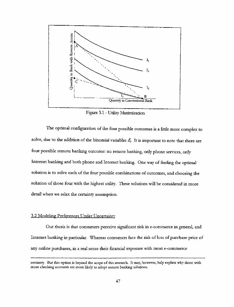
Figure 3.1 - UtiHty Maximization
The optimal configuration of the four possible outcomes is a Httie more complex to
solve, due to the addition of the binomial variables S-. It is knportant to note that there are
four possible remote banking outcome: no remote banking, only phone services, only
Internet banking and both phone and Internet banking. One way of finding the optimal
solution is to solve each of the four possible combinations of outcomes, and choosing the
solution of those four with the highest utiHty. These solutions wUl be considered in more
detaU when we relax the certaintj' assumption.
3.2 Modeling Preferences Under Uncertaint}"
Our diesis is that consumers perceive significant risk in e-commerce in general, and
Internet banking in particular. Whereas consumers face the risk of loss of purchase price of
any online purchases, in a real sense thek financial exposure with most e-commerce
certainty. But this option is beyond the scope of this research. It may, however, help explain why those with more checking accounts are more likely to adopt remote banking solutions.
47
transactions is Hmited by current credit card laws. In a sense, bankmg is also guaranteed,
smce any unaudiorized wididrawals from consumer accounts is covered by FDIC kisurance.
What is not covered by any kisurance is to the mvasion of very private mformation. And
smce banks serve as kiformation processors ki tiie economy, if security could be
compromised, tiiieves would have enough kiformation to steal not just deposits, but also
customers' identities. To adjust our model to aUow for uncertainty, we adjust assumption
A l ' Nature of Uncertainty: Consumers maintain certamty about thek abUity to use the new
technology. However, now we relax the assumption about security on access to thek
accounts. This assumption, therefore, knpHes a change only in the utUity function
associated with bank R, and only concerning the remote access segment. The nature
of the uncertainty itself may differ depending on the remote access service being
used. We assume now k distinct possible outcomes to security breaches for the
phone and Internet banking services. Some of these outcomes only affect one
service. The first outcome (/ = 1) is the same outcome assumed under certainty.
Further we assume that each consumer assigns a subjective probabihty {p) to each
outcome, constraining the svmimation of aU of these subjective probabihties to unity.
IiutiaUy, it is fiirther assumed that these probabihties are based on pubhcly available
information, and that markets are efficient in assessing these probabihties; therefore,
each consumer has assessed the exact same distribution to the possible ovitcomes,
which is a common theoretical assumption. Assuming an identical subjective
probabihty set for aU market participants aUows us to estimate a simpler model, and
wUl be relaxed later to examine the role of subjective risk assessment. This
assumption is unnecessary to theoreticaUy explain the role of subjective probabihty.
48
For notational convenience, it is further assumed that aU outcomes other than the
fkst outcome (/> /) result in lower utility, and that the disutihty grows, the more
money that is deposited in the remote accessible account (i.e.,^<0, g'<0 V />/) .
Because each g^<0 under uncertainty, it is assumed that overaU utiHty of wiU be
strictiy less than utihty under the certainty assumption. And since utiHty has become
expected utihty, either a horrible outcome and/or a high probabihty of such adverse
outcomes (i.e., personal information theft) could cause the expected utihty to differ
gready from the utiHty under certainty.
A3' The thkd assumption would have to be altered to account for the other possible
outcomes, since aU k outcomes would need to be taken into account Using the
equations and relationships from the certainty model, the overaU utiHty is:
U(x) = pJ(x)^Y.p\hA,(^)^^2h2,(x)\. (3.4) i=2
Therefore, to be maximized could be re-written as foUows:
k *
U{x,y) = f{x) + Y.Pif^y) + P^^My) + PxS2h2{y) + YSi
where T^ = p; [SjA,_ (y)+82^, (j)\ ^o^ U k outcomes.
Skice aUj6,'s sum to one, this Ufx/^) can be rewritten as:
U{x, y) = fix) + f{y)+{5, h, {y) + 5^ h (7)]+
The MRS can be rewritten as:
£ r , -{\-p,)5My)-{^-Px)^i^^^y'^ (3.5) V'=2 J
49
MRS = ^ ^
/•+[^A'+^2'^2']- E r / -{i-p,)s,h,'+{i-pXh2' .1=2 J
(3.6)
Note that except for the last square bracket, Equation 3.5 is the same as Equation
3.2 under certahity. Also, note tiiat if/), is 1 (therefore aU other;!)^ are zero), the MRS is the
same as that discussed in the model under certaintJ^ Also if both of the terms ki square
brackets in 3.6 are zero, the MRS is 1 for aU values of x a n d j , and if remote banking is no
more costiy than conventional banking, then the consumer would again be indifferent
Interpreting the imphcarions of the model under uncertainty requkes that we
interpret the terms in square brackets in 3.6. The first term in square brackets in the
denominator of 3.6 represents the added utihty of the remote banking services under
certainty. The term in the second square bracket represents the consumer's risk premium.
This definition is obvious when Equation 3.3 is compared to 3.6. The only added
component is the last square bracket. If it were not for that square bracket the two MRS
formulae would be equal. The risk premium wUl be explained in greater detaU in the
foUowing section.
3.3 The Role of Risk Aversion on Adoption Decisions
Before interpreting the last square bracket in Equation 3.6, we need to quickly review
the derivation of what is commonly regarded as risk aversion. Pratt derived that measure ki a
landmark article ki 1964. The focus of what he caUed "relative risk aversion" came from his
focus on what he caUed a risk premivim. The risk premium {it) was defined as a premium
50
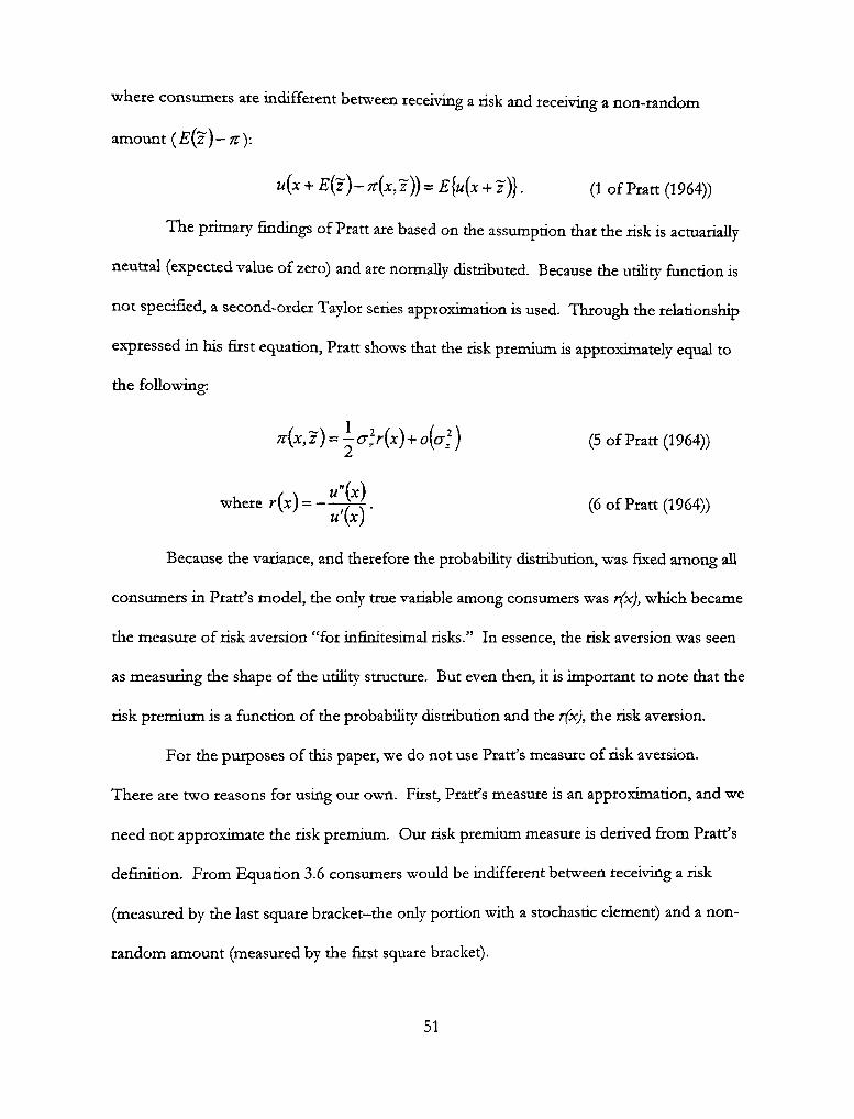
where consumers are hidifferent between receivkig a risk and receiving a non-random
amount ( £ ( z ) — K):
u{x -I- E{Z)- 7v{x,zyj = E{U(X + z)]. (1 of Pratt (1964))
The primarjf findings of Pratt are based on the assumption that the risk is actuariaUy
neutral (expected value of zero) and are normaUy distributed. Because the utiHty function is
not specified, a second-order Taylor series approxknation is used. Through the relationship
expressed in his first equation, Pratt shows that the risk premium is approximately equal to
the foUowing:
7r(x, z ) = - C7>(x) + o[c7l) (5 of Pratt (1964))
where r{x) = j ^ . (6 of Pratt (1964))
Because the variance, and therefore the probabUity distribution, was fixed among aU
consumers in Pratt's model, the only true variable among consumers was r(x), which became
the measure of risk aversion "for infinitesimal risks." In essence, the risk aversion was seen
as measviring the shape of the utihty structure. But even then, it is important to note that the
risk premium is a fiinction of the probabihty distribution and the r(x), the risk aversion.
For the purposes of this paper, we do not use Pratt's measure of risk aversion.
There are two reasons for using our own. Fkst, Pratt's measure is an approximation, and we
need not approximate the risk premium. Our risk premium measure is derived fiom Pratt's
definition. From Equation 3.6 consumers would be indifferent between receiving a risk
(measured by the last square bracket-the only portion with a stochastic element) and a non-
random amount (measured by the first square bracket).
51
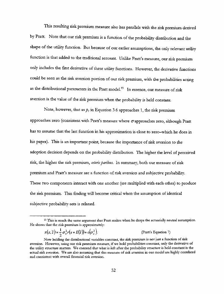
This resulting risk premium measure also has paraUels witii die risk premium derived
by Pratt. Note diat our risk premium is a function of die probabUity distribution and die
shape of die utiHty fiinction. But because of our earher assumptions, die only relevant utiHty
fiinction is diat added to the traditional account. Unhke Pratt's measure, our risk premium
only hicludes tiie first derivative of tiiese utiHty functions. However, tiie derivative fiinctions
could be seen as the risk aversion portion of our risk premium, with the probabUities actkig
as the distributional parameters m die Pratt model." In essence, our measure of risk
aversion is the value of the risk premium when the probabUity is held constant
Note, however, that as^ , in Equation 3.6 approaches 1, the risk premium
approaches zero (consistent with Pratt's measure where C7 approaches zero, although Pratt
has to assume that the last fimction in his approximation is close to zero-which he does ki
his paper). This is an important point, because the importance of risk aversion to the
adoption decision depends on the probabUity distribution. The higher the level of perceived
risk, the higher the risk premium, ceteris paribus. In summary, both our measure of risk
premium and Pratt's measure are a fiinction of risk aversion and subjective probabihty.
These two components interact with one another (are multiphed with each other) to produce
the risk premivim. This finding wUl become critical when the assumption of identical
subjective probabihty sets is relaxed.
" This is much the same argument that Pratt makes when he drops the actuarially neutral assumption. He shows that the risk premium is approximately:
7c{x, 2 ) = — cr^A-(x + £(2))+ o\al). (Pratt's Equation 7)
Now holding the distributional variables constant, the risk prenuum is not just a function of risk aversion. However, using our risk premium measure, if we hold probabilities constant, only the derivative of the utility structure matters. We contend that what is left after the probability structure is held constant is the actual risk aversion. We are also assuming that this measure of risk aversion in our model are highly correlated and consistent with overall financial risk aversion.
52
The second reason our risk premium measure is more appropriate for our case is
that it adapts easUy to our distribution channel analysis. Pratt's equation is a good
approximation for continuous functions, where we are interested about changes in utility
over a infinitesimaUy smaU increase in risk. However, as we pointed out earher, our utility
function includes variables ^, and ^p, which are either zero or one, making the function
discontinuous at those points. In addition, the budget constraint also adds discontinuity to
our model.
To Ulustrate this difference and more closely approximate the distribution channel
decision of most consumers, we generalize the model presented thus far with the foUowing
utihty function. As the consumer looks at where they are now, and consider the remote
access distribution configuration they propose, they would act as if they calculated one of the
foUowing MRS (restated in the form of Equation 3.6):
/ • MRS Tmd—>Phone
MRS Trad-^lnlcmel
HK] + MRS
[1 \i=2
Zr;.-u.=o - ( I - A K
Phone-*Phone I Inl
MK^K] + Ir;,,,,.,J-(i-P,K+(i-A)^2 1=2
(3.6a)
(3.6b)
(3.6c)
53
z'+te] + MRS
( k
V'=2 J Inlemel-*Phone I Inl
f+lK + Kh (*
V ir,;,_.,..,=i]-(i-;',K + (i-A>;
(3.6d)
If the consumer is aware of only one of these two services (or only one is offered
from the bank), then the only possibUities are the traditional service or the one remote
service. The consumer then wovUd act as if they calcvUate either phone or Internet banking
MRS (Equations 3.6a or 3.6b). As one becomes aware of the other service (or the bank
begins offering the other remote service), then depending on which service has akeady been
chosen, the consumer would act as if they calculate one of the other MRS (Equations 3.6a
through 3.6d), To determine whether the MRS is greater or less than 1 (the point of
indifference between to channels if costs are equal) depends only on the sum of the last two
square brackets. If the sum of the square brackets m the denominator is greater than the
sum of square brackets in the numerator (or greater than zero in the case of 3.6a or 3.6b),
then the consumer wiU choose to expand thek channels of banking services. In short,
consumers wUl accept the new distribution channel as long as the potential utUity gain
exceeds the risk premium.
It should be noted that m aU cases, die customer may meet a different budget
constraint as one moves from one remote access channel to another. For example,
consumers without a computer would find k expensive moving from phone to Internet
banking.
54
3.4 Theoretical Summary
From die models presented in diis chapter, we would expect that remote bankmg
adoption is a fiinction of tiiree concepts. Fkst, it depends on die added utihty offered. The
greater die added utiHty, tiie more hkely it wUl be adopted. The higher die benefit to die
consumer, tiie higher the adoption rate should be (positive relationship).
Second, adoption depends on the marginal cost to the consumer. This concept
refers to die budget constrakit in die model. The existence of a fee wUl discourage adoption
(negative relationship). The more consumer costs that are sunk and the lower the marginal
cost, the higher the adoption rate should be (positive relationship).
Thkd, it depends on the risk premium, which is made up of subjective probabihty
function of consumers and the shape of the utihty functions, which we have shown is risk
aversion. The less Hkely security breaches are perceived to cause bad outcomes, the more
Hkely consumers wiU adopt remote banking services. We wiU ioitiaUy assume identical
probabUity distribution expectations across aU bank customers at any given time. This
concept is much more important in the case of Internet banking because it does not have as
long a history over which the long-term probabUity of security breaches has been estimated.
And finaUy, adoption depends on the nature and shape of the utiHty fiinctions.
Another way of looking at that shape could be the risk aversion of the consumer in general.
Since risk aversion and subjective probabihty interact, the larger the subjective probabihty,
the more important risk aversion is in predicting what remote channel decision wiU be made.
Under an kutial assumption of identical subjective probabihties for aU participants in the
market for bankkig services, the shape of the utiHty function becomes most important in
assessing the adoption, the higher the risk aversion, the lower the adoption rate should be
55
(negative relationship). In essence, the more sensitive the adoption rate is to the risk
aversion variable, the higher the perceived risk.
As the identical subjective probabihty distribution assumption is relaxed, we wiU then
begin to explore what factors may cause consumers to experience lower levels of perceived
risk. Many of the factors that affect requked human capital investment also affect ones
experience widi electronic commerce. These factors could also affect the subjective
probabihty distribution. If individuals have different subjective probabUities, then banks can
aim at affecting them dkecdy.
56
CHAPTER 4
DATA AND METHODOLOGY
To test the impHcations of the model presented in the previous chapter, we use data
from tiie 1998 Survey of Consumer Fkiances (SCF) sponsored by the Board of Governors
of the Federal Reserve System. The SCF is conducted every three years. This survey was
conducted by the National Opinion Research Center at the University of Chicago.'" The
SCF is a national survey, conducted in person by an interviewer who keys responses dkecdy
into a laptop computer. The computer also helps standardize the way the lengthy survey is
conducted.
The survey is sampled in two steps. Fkst, a geographicaUy based random sample is
taken. This first sample is designed to capture the asset and liabUity characteristics of the
overaU population. The second sample is selected to disproportionately represent those
households with more wealth. This sample is taken firom tax data (conducted in cooperation
with the Treasury Department-more specificaUy the Internal Revenue Service). The 1998
survey included responses from 4,309 households, 2,813 from the general random sample
and 1,496 from the wealthier weighted sample.
The interview took a median of 1 Vt hours per household, although it could take
substantiaUy longer depending on the complexity of the household's finances. Of those
being randomly selected, not aU consented to taking the survey. The response rate for the
general portion of the sample was 70%, and 35% for the tax hst sample.
w For more information about the mediodology used or descriptive statistics from the 1998 SCF see Kennickell, Starr-McClueer, and Surette (2000).
57
The Federal Reserve makes this data available to researchers in a "pubhc access" data
set. To preserve confidentiaHty four observations were dropped. To preserve the
confidentiahty of the remaining observations, financial data (such as income and deposit
amounts) were reported with a randomized disturbance added. To partiaUy compensate for
the added noise, this data set was rephcated five times. AU analyses run in this paper wUl be
conducted on aU five repHcations together, weighting each observation to account for both
the over-sampling and repHcations.
To adjust for the over-sampling problem we need to use a weight variable provided
in the database. A Consistent Weight variable is estimated by the Federal Reserve, based on
how many households in the overaU population are represented by that observation. The
total of aU consistent weight households sums to 102.5 miUion (for each repHcation).'^ To
account for both the repHcations and the over-sampling, observations wiU be weighted by a
variable caUed Sample Weight, which is calculated as:
Consistent Weight x 4,305 Sample Weight = ^ 1 .
^ ^ 102.5mUhonx5
The 4,305 in the numerator is the actual number of observations ki the 1998 sample.
But not aU households wUl be used. The focus of this paper is why bank customers
choose to engage in Internet banking. Therefore only those households who do business
with a bank are kicluded in the dataset and the analysis tiiat is outhned below. In 1998, 94%
of aU households (4,058 households) surveyed were bank customers, so diere is Httie loss of
'5 The base for diis design is discussed by Kennickell and Woodbum (1999). There is an updated mediodology discussed by Kennickell (1999). One is merely a refinement of die odier, and almost certainly will not make any difference to die outcome of our tests. We will use die weights based on the updated methodology.
58
sample size. The weighted sample size may be different though. In essence, the sample
weight for non-bank customers is set to zero.
Although not a common data source, the SCF has been used to analyze wealth,
income and financial economic questions. As a data source for those appHcations, it is weU
accepted. Juster and Kuester (1991) compared several data sources used in the hterature to
analyze wealth, wealth inequahty and wealth composition."^ SpecificaUy, they reviewed the
National Longimdinal Survey of Mature Men and Retkement History Survey, specificaUy
comparing them to the SCF for 1983. Despite the fact that the SCF was restricted to the
same sub-sample as these narrower surveys, Juster and Kuester found that the SCF had
fewer missing values, and less attrition in the taUs of the income distribution (both high
income and low income but more pronounced in the upper tail). The primary reason for
better results seems to be the emphasis that the SCF places on the oversample in the upper
income area. They also estimate the weights that could be used for unbiased econometric
estimation.
Wolff (1992) used the SCF from 1983 and 1986, as weU as die Survey of Fkiancial
Characteristics of Consumers from 1962 to show how wealth mequahty had changed over
time. These two years were used because an attempt was made to resurvey the same set of
households m 1986 as were surveyed in 1983. In addition to tiie SCF, tiie Survey of Income
and Program Participation (SIPP) was used for tiie years 1984 and 1988. The SIPP also
surveyed die same households, but Wolff was only able to use tabular data from dus source,
not die underlykig data itself He compared wealdi equahty overtime usmg Gmi coefficients,
which were srniUar uskig SIPP or SCF. Witii die SCF, he also was able to use regression
A similar finding was reported in Curtin, Justin, and Morgan (1989).
59

models. Over longer periods of time he compares die Survey of Financial Characteristics of
Consumers (SFCC) from 1962 witii die SCF of 1983 to see how wealdi mequahty has
changed over time. He found an increasing wealdi inequahty in the 1980s, controUing for
kicome, and many other variables. Much of this is due to "fortuitous economic
ckcumstances" for those bom between 1914 and 1938. He found that household
kidebtedness rose from die 1960s to the 1980s. Black households saw greater wealdi gams
over that time period, but stiU traU white households. Usmg these and other sources, Wolff
found that much of the wealth gain by black households was caused by inter-generational
wealth transfer.
Mulhgan (1999) also examined the inequahty of wealth. He too looked at the
persistence of inequahty as it related to inheritance. He contrasted the Galton model with a
human capital model to explain the regression to mean wealth observed over generations.
His model assumes some abihty to generate wealth is passed on to future generations
biologicaUy (geneticaUy) and that given higher wealth, that innate abihty is further developed
by the abUity to gain human capital through education. He presents a model, which explains
the persistence of inter-generational wealth transfer and the eventual regression to the mean
observed in the data. He used data fiom the Panel Study of Income Dynamics, the 1989
SCF and the National Longitudinal Study of Youth to test the imphcarions of the original
Becker-Tomes model, as weU as he extension. The prevaUing models (as weU as his own)
predicted that borrowing constrained famUies would act differentiy than those not
constrakied. Therefore, to MuUigan, die fact tiiat wealtiiy households were "over-sampled"
in the SCF was an advantage of that dataset.
60
Cox and JappeUi (1993) used die household balance sheet data firom die 1983 SCF to
analyze die effects of borrowing constrakits on household HabUities, and more knportantiy
the significance of those constraints ki previous research on household liabUity. They were
able to separate those with borrowing constrakits from those without by dkect questions
asked ki the survey. They use a three-equation generalized Tobit model to test thek
hypothesis. Unhke Mulhgan, Cox and JappeUi wanted a representative sample of the
population, so they excluded 438 high-income respondents, leaving them with a sample size
of 3,691. To show that the Tobit model holds, diey fkst show that two of the equations
hold separately (these were latent variables used in the generalized Tobit) using a Probit
model. FinaUy they used the three-equation Tobit model, which also held. Cox and JappeUi
find evidence of constraints to borrowing, primarily Hquidity constraints not normaUy
included in borrowing models. They estimate that removing these constraints would
increase borrowing by nine percent, which might affect some of the current models'
accuracy.
Crook (2001) used the 1995 SCF data to analyze the demand for household
borrowings, given the likely supply of borrowing for the household (determined in the
model by the Hkehhood of being rejected for borrowing). There are two aspects to finding
the amovmt of borrowing taken on by a household. Fkst, a model is presented to determhie
the borrowing consttahits. And second, the demand is estimated given any borrowing
constraints. The 1995 SCF "over-samples" wealtiiy households. This research question
would best be addressed uskig a random sample. To adjust for the wealth bias. Crook trims
the dataset of any observation where income is greater tiian $300,000 and assets are greater
dian $1 mUHon. The 1995 SCF contains 4,299 households, and the sample acmaUy used
61
contains 3,199 households, which would imply that 1,100 households were trimmed. Due to
lack of observations in some of his variables, the useable sample for much of the Probit and
regression models run dropped to 2,578. For the most part, his model supported general
findings of earher models, with subtie differences.
Gale and Scholz (1995) used die 1983 and 1986 SCF to analyze die effect of IRA
contribution limits on the private and national savings hmits. As in the Wolff article, the
1983-1986 SCF was used because diey tried to coUect data fiom the same random sample
over those two years so that change variables were meaningful. They compare some
findings with IRS Micro-data to demonstrate the accuracy of the SCF. They included in
thek descriptive statistics, SCF descriptive demographic statistics by IRA, non-IRA and IRA
contributions to the limit. Thek sample was also trimmed. They excluded households
where the head of household was younger than 24, the marital status changed between 1983
and 1986, the head of household or spouse was self-employed, or was over 65. They further
trimmed to reduce the "extreme range of saving in the sample," by dropping any
observation where the absolute value of saving or dissaving was greater than $100,000. This
is where the difference over the 1983-1986 time fiame comes ki. A system of regression of
equations are then estimated usmg OLS and maxknum hkehhood estimates. These estimates
are used to model the amount of mcrease m savings that would have been reahzed by
kicreaskig IRA hmits. Gale and Scholz found tiiat Htde additional savings would have been
reahzed from 1983-1986 had higher Hmits been m effect But diey admit diat die trimmmg
of the oudying savers is econometricaUy troubhng.
Calem and Mester (1995) used die 1989 SCF to analyze why credit card mterest rates
do not foUow die normal assumptions of price behavior under perfect competition. They
62
use tiiree hypotiieses firom die Hterature on die subject: consumer face search costs,
consumers face switchhig costs, and issuers face adverse-selection problems if they
unUateraUy reduce kiterest rates. Calem and Mester use a sub-set of die 1989 SCF, uskig
1,661 households, tiiose widi at least one type of bank-type credit card. They propose a
model where credit card borrowmg is a function of die household's propensity to shop for
die best terms on large purchases, the household's attitude toward installment credit in
general, attitude toward borrowing for vacation, and attitude toward borrowing for purchase
of jewehry. Each of tiiese concepts was further broken kito variables that could be found ki
the survey. In addition to this model, two other Probit models were estimated for being
turned down for credit over the past five years, and experiencing repayment difficulty.
Using these models, they were able to find support for the three hypotheses mentioned
above.
Duca and WhiteseU (1995) used die 1983 SCF to examkie die effect of credit card
ownership on the demand for money. They show that the relationship between credit card
usage and cash may be negative because consumers would have to hold lower precautionary
balances, fiinds used for transactions could be held in assets with higher yield than checking
accounts whUe waiting for the bUl, and/or consumers may synchronize payments with
paychecks, reducing the need to carry cash. Arguments covUd also be made for positive
correlation with credit cards and cash holdings, there may be fewer withdrawls from
checking if credit cards are used-thereby increasing the balance, if checks and cards are
substimtes then balances may grow if there is a cost of converting checking balances to
higher earning assets, and card holding may reveal (or signal) a higher propensit)'^ to
consume—resulting in a higher demand for cash. They used a probit methodology to model
63
account configuration decisions (checking account, savings account, etc.), and a regression
methodology to estimate the impact of the credit card decision on the money demand.
Although the main focus of the paper was on demand, they constrained the model by
probable loan availabUity (supply factors). Both were found to be important in the amount
of cash held vis-a-vis credit balances. They found tiiat the overaU relationship between
transaction accovmts and credit cards is negative.
Starr-McCluer (1996) used the 1989 SCF to examine the connection between savings
levels (as precautionary savings) and health insurance. If consumers have health insurance, it
is expected that they wiU hold less precautionary savings. Starr-McCluer acknowledges that
the 1989 SCF oversampled 866 wealthy households of the 3,143 in the sample. But since
she is interested in explaining wealth holdings by health insurance as weU as insurance
coverage by wealth, the added variabUity is not accounted for by trimming. She finds mixed
evidence in favor of the hypothesis of a negative relationship between precautionary savings
and health insurance, and in fact using a regression analysis she shows that the amount of
insurance and savings are, in fact, positively correlated, even after controlling for other
variables such as age, education, health problems, edinicity, and income. The one variable
not accounted for hi this model that might help explain some variation is risk aversion,
which we wiU show that the dataset contains.
Gale (1998) used the 1983 SCF to re-analyze how households offset pension wealtii
by tiiek accumulation of overaU wealtii. Past estimates have suffered fiom metiiodological
biases, and Gale shows tiiat previous metiiodologies understate die offset He used die SCF
because k contams household balance sheet, kicome and demographic data, as weU as very
detaUed kiformation about household pensions. The sample used uicluded only tiiose
64
respondents where the head of household was between 40 and 64, worked more than 1,000
hours per year, defined that as workkig fiiU-time, and neitiier spouse was self-employed. The
younger households were excluded due to kicomplete pension data. The resulting sample
was only 638 households. Gale demonstrates that offsets between pension and non-pension
wealth have been systematicaUy understated. However, the results may not be extrapolated
to the general population because the survey contains a higher than average (median) weight
of wealthy households.
Heaton and Lucas (2000) used data fiom die 1989,1992 and 1995 SCFs to knprove
upon asset-pricing models that use income. One attempt at improving the CAPM has been
to add wage data, assuming that variabUity of salary is important in choosing asset/portfoHo
risk. Heaton and Lucas expand this model to include proprietary income. They use two
models and two datasets. The first uses the SCF (for regression only the 1995 data are used).
They exclude observations where households held less than $500 in stock or less than
$10,000 net worth in financial assets. It is imclear fiom the paper how large thek sample
size was, since aU tables report only "imputed" number of households (unless they used a
bootstrapped sample). A bootstrapped sample has the benefit of weighting the households
proportionaUy to the population. This model was used to show that the amount of risky
assets is a function of proprietary income-the higher the proprietary income, the less added
risk was taken on through stocks. This paper would also have benefited firom adding the
risk aversion variable available in the dataset. The second model was more of a macro
model that used models aggregate stock market wealth, human capital and proprietary
income. This model used the Tax Model data. The model found support for the general
65
hypotiiesis of addkig proprietary income as a more complete CAPM, smce non-pubhcly
traded company holdmgs are tiieoreticaUy kicluded m the capital assets of the CAPM.
In summary, die SCF has typicaUy been used to address wealdi, kicome and
consumer financial economic problems. Many appHcations have focused on aggregate
demand or demand effects. It is typicaUy used in a cross-sectional analysis. And it is best
used when the over-sampling of wealthy households is not a disadvantage in the final
inferences or when economic weights can be apphed to the results to correct for i t
4.1 Variable Description
Households were asked about the financial institutions they used and the ways they
interacted with them. The Hst of institutions avaUable for these responses was quite
extensive. The primary types of institutions included commercial banks, savings and loans
(or sa\Tngs banks), credit unions, finance or loan companies, and brokerages (and mutual
funds). However, this is not an exhaustive Hst by any means.
Each time a respondent identified a financial institution used by a member of the
household, they would be asked the primary ways they interact with that institution. Again,
many options were given. We categorized the household as using e-banking if one of the
responses to that question was computer, Internet or online service for a commercial bank, savings
& loan or credit union. Phone-banking was asked twice. One possible response was
phone(talking), and the other ^"is phone(touchtone). We use each of these separately, as weU as a
thkd variable that is at least one tj^e of phone banking.
The theory described ki the last chapter imphes that Internet bankmg adoption is a
function of utihty added by adoption of remote banking services, budget constraint (added
66
cost), and the expected disutihty in adopting remote banking services. As mentioned in the
previous chapter, we assume that aU banking customers expect the same subjective
probabUity distribution for aU possible outcomes. This homogeneity of subjective probabihty
distribution holds across aU customers and for aU banks.
To proxy for the added utiHty of the remote banking services we use characteristics
of bank accounts. It was assumed that those benefiting most fiom Internet bank
management services would be those who had the most complex banking relationship. To
measure complexity, we used number of savings accounts, and number of checking accounts
(Xj in the models in this chapter and # Checking in the tabular results). The number of
savings accounts was not asked dkecdy. The SCF does, however, ask how much
respondents have in savings, account by account. So the number of savings accounts is
merely the sum of savings account balances greater than zero (X, in the models presented
hereafter, and # Savings in the tabular results).
Another possible proxy for utihty is the amount of money kept in very hquid
accounts, checkmg and savings (X^ in the models in this chapter, and $ Liquid ID. the tabular
results). If one keeps more money m these accovmts, Internet management may become
more useful. Respondents were asked to report on the amount held in checking and savings
at the time of the kiterview. But tiiis variable is complex, smce die more one has ki tiiese
accounts, the more is at risk if security is breached.
As discussed ki the last chapter, die variables knportant to die budget constramt are
diose diat kicrease die cost of remote bankmg, costs tiiat are not aheady sunk. These are die
costs diat make the slope of the budget constraint ki Figure 3.1 flatter tiian 1. Skice
computer Hteracy is an important portion in tiie budget constraint described in the last
67
chapter for either touchtone phone-banking or Internet bankkig, the next set of variables
address that cost. To proxy for the budget constraint we used income, education and age.
The survey did not ask about computer hteracy, but it did ask about diek level of education.
Through several questions, respondents (head of household and spouse) were asked about
thek highest level of education and thek coUege degrees. We used only the response for the
"head of household." We spht thek responses into the foUowing categories: less than high
school, high school graduate, some coUege, bachelor's degree, masters degree, and doctorate
degree {d, through d; respectively for the models, dropping bachelor's degree-A/Hi", HS SC,
MA and DR, respectively, for the tabular results).
FamUiarization with Internet financial services can be judged by looking at other
financial services, which the consumer accesses via the Internet We use the dummy variable
a to indicate if other financial service is accessed via the Internet (Familiarity in the tabular
results).
The other variable that may be relevant in assessing thek computer Hteracy is thek
age (the head of household again), which was taken as given (X^ for the models in this
chapter, ^^f for the tabular results). The svirvey asked thek birth date, and thek age-then
reconcUed them. In using this variable, it is assumed that the older the consumer, the less
Hkely they are to have received computer training in school. And since Internet banking
assumes some computer hteracy, it is assumed that the older one is, the less hkely one is to
have mvested ki this human capital. It is unclear how human capital variables affect phone-
banking. Touchtone phone-bankmg aUows customers to interact witii die computer tiirough
thek phone, and resembles a menu driven program. Those with a computer backgrotmds
also may be more Hkely to adopt touchtone banking as weU.
68
FmaUy, die natural log of mcome was used (X^ for models ki tiks chapter, ln(Income)
was used for tiie tabular results). Household mcome was asked dkecdy, and was asked m
pieces (i.e., how much did you earn in salary, mterest, etc.). The pieces were tiien summed
and die two versions (dkect question and die sum of the pieces) reconcUed. For those
reporting a negative hicome, tiie computer program kiput a - 1 . We dropped tiiese
observations shice the negative amount was unknown. From a budget constrakit
standpokit, it is assumed that the more money one earns, the more Hkely one has aheady
invested in a computer (from the Internet bankmg standpokit).
The survey did not address the cost of the onhne service, the e-banking service, or
any phone-banking charges. The models used m this chapter, in essence, assume that these
are zero.
4.1.1 Differing Degrees of Risk Aversion
Subjective probabUity distribution was not asked, and is not observable dkecdy
through this dataset. As mentioned in the theory chapter, the subjective probabihty is
assumed to be identical across aU consumers. Since the risk premium is a fiinction of both
the subjective probabihty and the risk aversion, we turn our attention now to risk aversion.
Risk aversion was asked dkecdy. Respondents were shown a card with the foUowing
four options and asked "Which of the statements on this page comes closest to the amount
of financial risk that you and your (spouse/partner) are wUling to take when you save or
make investments?" Then each subject was shown a card with the foUowing options:
1. Take substantial financial risks expecting to earn substantial retiums.
69

2. Take above average financial risks expecting to earn above average retvuns.
3. Take average financial risks expecting to earn average retvims.
4. Not wiUing to take any financial risks.
The response was coded with die number of the response given (for models in this chapter
these responses take on the values of 5, through 4 , the tabular results use riski through
m/fe-^-although usuaUy the last measure is dropped in the regression).
Risk aversion is a function of the shape of consumers' utiHty functions. As such, the
added utiHty, and the expected disutihty discussed in the last chapter should be a function of
that same utihty function.
As described above, some of the data were rephcated to protect the identity of the
respondents. But not aU variables were equaUy affected by this rephcation. Of aU of the
variables described in this chapter, the income variable and amount held in checking/savings
accounts were affected most by the repHcations. The number of accounts, age, education,
and risk aversion were changed by repHcations in fewer than a dozen cases, which affected
descriptive statistics in these variables at the one-thousandths level (the descriptive statistics
for these variables were virmaUy unaffected by these repHcations).
4.2 Base Model Development
The model presented in Chapter 3 poses certahi esthnation chaUenges. Fkst, the
functional form is not specified because there is no agreement in the hterature on what form
it should take. And even if the functional form were known, theory suggests that each
person could have different set of coefficient values making utUity difficult to model. To
70

avoid diese problems, we focus on consumer preference revealed through the adoption
decision.
The purpose of the tests in this chapter is twofold. Fkst, we wish to show that the
decision can be described uskig a bivariate logistic regression model. This model is
consistent with Equations 3.6a and 3.6b hi the theory chapter. Using the variables discussed
in this chapter, we would proxy marginal utihty by number of checking and savings accounts,
as weU as the total doUar value held in those hquid assets. The margmal cost would be
proxied by income, age, education and whether they currentiy use the Internet for financial
services outside of banking. The risk premium is proxied by risk aversion (initiaUy-holding
subjective probabihty constant across aU consumers).
Second, we wish to find an adequate parsimonious model that can be used in
multinomial test in the next phases. Using the statements in the summary of Chapter 3, we
can conclude that this model hypothesizes the foUowing about phone banking, 9, (a
binontkal variable, either adopt or not):
9^ =f{h„T]i,tpJ, (Empirical version of 3.6a)
Where /&, = the utihty added by phone banking (the value of the first
bracketed term in the denominator of 3.6a with J = 0)
;;, = the budget constraint with an phone banking (the value of the
budget constraint with ^ = 0)
(p, = the expected disutihty by adding phone banldng (the value of
the second bracketed term ki the denominator of 3.6a with ^ = 0).
A simUar relationship should exist for Internet bankkig:
71

^2~f ^2> "Hi' 2) y (Empirical version of 7b)
WTiere hy — the utiHty added by Internet banking services (the value of the
first bracketed term in the denominator of 3.6a with 5-^ — 0)
r]2 — the budget constraint with Internet banking (the value of the
budget constraint with 5^ — 0)
^, = the expected disutihty by adding Internet banking (the value of
the second bracketed term in the denominator of 3.6a with 4 = 0).
To test the appropriateness of this model methodology we wiU use the foUowkig
base model:
3 e
71 = 1 + /
where
^h = t p A ^ , +IP..45,X2 +ip..3S.X3 (4-1) ,=\ /.=] c=\
5
yri = y,X4 +73X3+ Iy,,2<. + Yga 1=1
where n - BemouUi probabUity of using phone or (Internet bankmg)
X, = Number of checking accounts held by household members.
X, = Number of savkigs accovmts held by household members.
X^ = Amount ki savings and checking accounts.
X# = Reported age of die "head of household."
X- = Natural log of reported income.
72
^= Dummy variables for level of education of the "head of
household." Education levels "No High School" tiirough
"Doctorate"-Bachelor's Degree is omitted (acts as base
education).
a = Dummy variable indicating whether or not other financial
services are accessed via the Internet.
dj= Dummy variables for the level of risk aversion reported for the
"head of household." Levels 1-4 described earher-"4" is
omitted (acts as base risk aversion) among the dummy variables
at the end of the equation.
/?^;^^= Coefficients to be estimated by the logistic regression.
This model aUows for the maximum amount of flexibihty. It aUows the variables
proxying for utihty to have a different effect depending on the shape of the utiHty function,
which is what the interaction term in the first set of summations is intended to capture.
Because the budget constraints are not affected by the shape of the utiHty function, no such
interaction is employed. Since we are, at this point, assuming identical subjective probabihty
sets, the effect of die risk premium would be picked up primarily in the last three
coefficients.
This aU leads to our first two hypotheses.
H,p: fii=...=Pn=7i----=76=^1-•••-^3^0 (phone bankkig adoption model)
H,,: /?,=... =Pu'=ri=- • • =n=^t=- • -=^3=0 (Internet Bankmg model)
73

If die model does work hi describkig die adoption decision, then hypotheses can be
specified about the sign of the coefficients. According to the theory described in Chapter 3,
we would expect the first three X-variables to proxy for the utiHty construct. We
hypothesize that the more complex a households financial accounts, the more utiHty gakied
through adoption of remote banking. And since the most volatUe account is the checkkig
account, greater utihty may be derived with households with many checking accounts, so
that they can manage account balances either online or via the phone. It is therefore
hypothesized that the coefficients for these variables would be positive. Amounts held in
savings and checking accounts proxy for amount of hquid assets held at a bank. It is
expected that the more invested in banks, the more Hkely it wiU be that they computerize
thek management of it, therefore dus variable is expected to be positive.
Another way of looking at demand for Hquid assets is the opportunity costs. From
this perspective, the higher the amount held in savings and checking, the more important it
is to manage those accounts. However, the coefficient for this hquid asset (sum of amount
held in savings and checking) could be found to be negative overaU, since as the amount
goes up, the more assets are held at risk of any security breach. Therefore the statement of
hypothesis wiU be stated weaker:
Hj : Number of checking accounts affects phone banking adoption y5,<0,
P2^,I3,^,P,^
Hj : Number of savmgs accounts affects phone baiUdng adoption P^<0,
/3,^,/3,<0, fi,^
74
H4p: Amount held in Hquid accounts affects phone bankmg adoption fig=0,
P,o=0, Pu=0, Pn=0
H^: Number of savkigs accounts affects Internet Banking adoption P,<0,
P2^,P,<[),P,^
Hjj: Amoimt held m Hquid accounts affects Internet Bankmg adoption Ps=0,
P,o=0, P„=0, P,2=0
These hypotheses are not meant to be taken jointiy. Rather than stating each of
these hypotheses separately, we have stated three hypotheses together. This convention wUl
be foUowed in future. Whenever hypotheses are separated by a comma, they are to be seen
as separate hj-potheses.
Age, income and education aU proxy for the budget constraint (at least for the
Internet banking channel). It is expected that the more money earned by households, the
more Hkely they are to have invested in a computer, thereby reducing the marginal costs of
using a home computer, and investing the time and money into being able to use a
computer. Therefore, a positive coefficient is expected on the income variable in the
Internet banking model. This same argument may hold for the touch-tone phone banking
(which mimics a menu driven computer system), but could not be made for voice phone
banking. No sign is hypothesized for voice phone banldng model (this variable may not be
significant for that model).
The age variable proxies for one aspect of human capital investment In this
context, age represents the experience the head of household has with computer technology.
It is expected that the older one is, the less training one received m uskig computers ha
75

general and die Internet ki particular. The hypodiesized coefficient on dus variable is
negative ki the Internet bankkig model. This same argument may hold for the touch-tone
phone banldng (which nkmics a menu driven computer system), but could not be tnade for
voice phone bankkig. No sign is hypothesized for voice phone banking model (this variable
may not be significant for that model).
The education dummy variables represent the classes No High School, High School
Graduate, Some College, Masters Degree and Doctorate levels, in that order. Bachelor's Degree was
dropped and acts as the base of analysis. We would expect those below coUege to have
negative coefficients. Since our model treats education as a sunk human capital cost, it is
unclear whether graduate degrees viiU add appreciably to the necessary capital to participate
in remote banking. These should be positive, but might not be statisticaUy significant, since
the amount of additional computer training in most graduate programs depends gready on
the graduate program. These same argument may hold for the touch-tone phone banking
(which mimics a menu driven computer system), but could not be made for voice phone
banking. No sign is hypothesized for voice phone banking model (this variable may not be
significant for that model).
If the household uses the Internet for another type of financial services, Internet
banking is more Hkely. There is no reason to beheve that famiharizarion with electronic
financial services wiU impact phone banking at aU.
H5 : Age affects touch-tone phone bankkig adoption y^>0.
Hfi : Income affects touch-tone phone bankmg adoption Y2^.
76
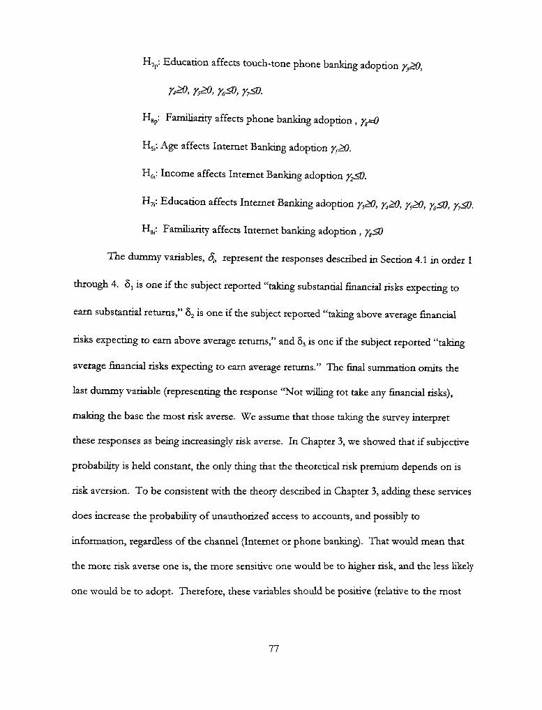
H^p: Education affects touch-tone phone bankmg adoption /j>0,
y,>0, rs>0, y,<0, y,<0.
Hgp: FamUiarity affects phone bankmg adoption , yg=0
H5,: Age affects Internet Banking adoption y>0.
Hg,: Income affects Internet Bankhig adoption y2<0.
Hyj: Education affects Internet Bankmg adoption y}>0, y^>0, y^>D, y^<0, yy<0.
Hg : FamUiarity affects Internet banking adoption, y^^H
The dummy variables, 5-, represent die responses described ki Section 4.1 m order 1
through 4. 6, is one if the subject reported "takmg substantial financial risks expecting to
earn substantial returns," 62 is one if the subject reported "takmg above average financial
risks expectkig to earn above average returns," and 63 is one if die subject reported "takmg
average financial risks expecting to earn average returns." The final summation omits the
last dummy variable (representing the response "Not wUhng tot take any financial risks),
making the base tiie most risk averse. We assume that those taking the survey interpret
these responses as being increasingly risk averse. In Chapter 3, we showed that if subjective
probabUity is held constant, the only thing that the theoretical risk premium depends on is
risk aversion. To be consistent with the theory described in Chapter 3, adding these services
does increase the probabihty of unauthorized access to accounts, and possibly to
information, regardless of the channel (Internet or phone banking). That would mean that
the more risk averse one is, the more sensitive one would be to higher risk, and the less hkely
one would be to adopt. Therefore, these variables should be positive (relative to the most
77
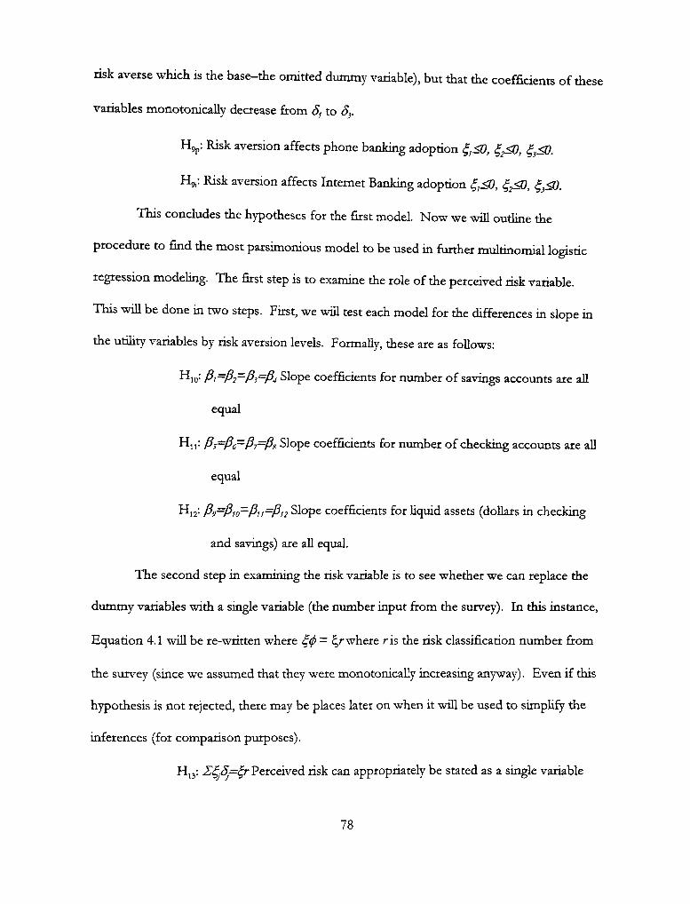
risk averse which is die base-tiie omitted dummy variable), but diat die coefficients of tiiese
variables monotonicaUy decrease fiom S^ to 6^.
Hgp: Risk aversion affects phone bankmg adoption ^,<0, ^^<0, ^j<0.
Hgj: Risk aversion affects Internet Bankmg adoption ^, <0, ^^<0, ^<0.
This concludes die hypotheses for the first model. Now we wUl outiine the
procedure to find die most parsknonious model to be used ki furtiier multinomial logistic
regression modeHng. The first step is to examkie die role of tiie perceived risk variable.
This wUl be done in two steps. Fkst, we wUl test each model for the differences m slope m
the utihty variables by risk aversion levels. FormaUy, these are as foUows:
^10- Pi=P2-p3=p4 Slope coefficients for number of savings accounts are aU
equal
Hi,: Ps^Pc-Pr-Ps Slope coefficients for number of checking accounts are aU
equal
^\2- P9-fiio~Pii=Pi2 Slope coefficients for Hquid assets (dollars in checking
and savings) are aU equal.
The second step in examining the risk variable is to see whether we can replace the
dummy variables with a single variable (the number input fiom the svurvey). In this instance.
Equation 4.1 wUl be re-written where ( ^ = 4^ where ris the risk classification number firom
the survey (since we assumed that they were monotonicaUy increasing anyway). Even if this
hypothesis is not rejected, there may be places later on when it wUl be used to simpHfy the
inferences (for comparison purposes).
H,3: i7^J—,^r Perceived risk can appropriately be stated as a single variable
78

This concludes the parsunonious testing of die model. It should be noted tiiat the
last two tests wUi be run on bodi models. If H,, is not rejected, H,g may be rerun to see if
kiteracting a single variable witii the utihty variables is more appropriate. From these tests, it
is hoped that a more parsimonious model tiian the original can be foimd to use in the
multinomial logit sections that foUow.
4.3 Functional Forms Test of the Base Model
The model wiU then be tested for functional form. Two tests are added to test for
the correcmess of the fiinctional form. The first examines only the budget constraint
portion of the model from Equation 4.1. Since it is hypothesized that Internet banking (and
possibly touch-tone phone banking adoption should be a function of computer hteracy
(sunk human capital investment), and since we use education and age to proxy for that
construct, we test to see whether adding an interaction term wiU add to the predictabihty of
the adoption. SpecificaUy, we rewrite yrj as foUows:
5 5
Fl = YiX^ -f-Y2X5 + 2 : Y , > 2 < + I Y * . 7 ^ ^ ^ 4 +Yi3a-
The term on the end is the interactive term. To test whether it adds to the
predictabihty of the model, we propose a fuU-reduced methodology testhig the foUowing
hypothesis:
H„: y8=yp=y 10=711=712=0 Interaction term does not add predictive power
The second test of functional form is testkig to see whetiier the logistic regression
should only consider non-Hnearities in the predictor variables. Shice k is not fuUy clear what
79
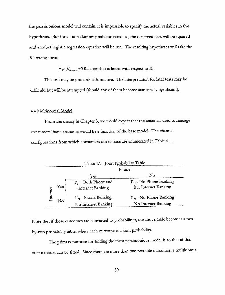
the parsimoiuous model wUl contain, it is impossible to specify the actual variables in this
hypothesis. But for aU non-dummy predictor variables, the observed data wiU be squared
and another logistic regression equation wUl be run. The resulting hypotheses wiU take the
foUowing form:
Hi 5: Px.,f„arr=0^^^^'i^onshxp is Hnear with respect to X.
This test may be primarily informative. The interpretation for later tests may be
difficult, but wUl be attempted (should any of them become statisticaUy significant).
4.4 Multinomial Model
From the theory ki Chapter 3, we would expect that the channels used to manage
consumers' bank accounts would be a function of the base model. The channel
configurations firom which consumers can choose are enumerated in Table 4.1.
tJ Yes c u B ^ No
Table 4.1 Joint Probabihty Table
Yes
P„ Both Phone and
Internet Banking
P21 Phone Bankkig,
No Internet Banking
Phone
No
P,2 - No Phone Banking But Internet Banking
P22 - No Phone Banking
No Internet Banking
Note tiiat if tiiese outcomes are converted to probabUities, tiie above table becomes a two-
by-two probabUity table, where each outcome is a jokit probabUity.
The primary purpose for findkig die most parsknonious model is so diat at tihs
step a model can be fitted. Skice tiiere are more tiian two possible outcomes, a multinomial
80
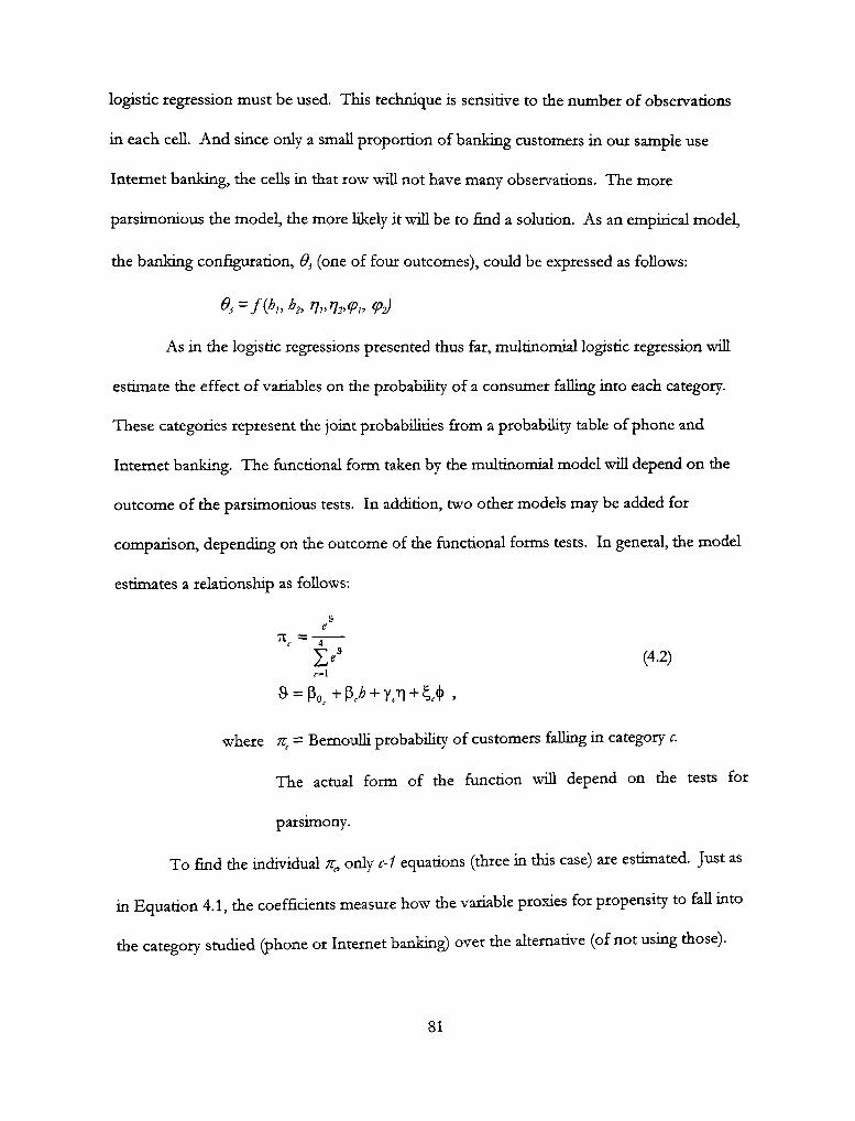
logistic regression must be used. This technique is sensitive to the nimiber of observations
in each ceU. And since only a smaU proportion of banking customers in our sample use
Internet bankkig, the ceUs in that row wiU not have many observations. The more
parsimonious the model, die more Hkely it wUl be to find a solution. As an empirical model,
the banking configuration, 9^ (one of four outcomes), could be expressed as foUows:
^3-I{^uKni''n2,(p„ (P2)
As in the logistic regressions presented thus far, multinomial logistic regression wUl
estimate the effect of variables on the probabihty of a consumer faUing into each category.
These categories represent the joint probabUities fiom a probabihty table of phone and
Internet banking. The functional form taken by the multinomial model wUl depend on the
outcome of the parsimonious tests. In addition, two other models may be added for
comparison, depending on the outcome of the functional forms tests. In general, the model
estimates a relationship as foUows:
7t. =
I^^ (4.2)
where K^ = BemouUi probabUity of customers faUkig in category c.
The actual form of tiie function wUl depend on die tests for
parsimony.
To fmd die kidividual ;r^ only c-1 equations (tiiree m diis case) are estimated. Just as
ki Equation 4.1, die coefficients measure how tiie variable proxies for propensity to faU mto
the category studied (phone or Internet bankkig) over die alternative (of not usmg diose).
81

Therefore if we defme the alternative to be neitiier phone nor Internet bankmg, then aU
coefficients and signs wiU be die same as tiiose hsted m Hypotheses 2 tiirough 7 above.
Again, we wovUd test die overaU model (die hypotiiesis diat aU coefficients are zero) uskig a
likelihood ratio test, which is the most important hypothesis at this juncture:
His: Pi--- • = A - 0 AU coefficients are zero (n because we do not know which
model wiU be used)
As mentioned above, a maxknum of two other multinomial models wUl be nm
depending on the tests of functional form. The coefficient signs of an expanded budget
constraint (with interactive age/education variables) would be similar to those in Hypotheses
2 through7. No coefficient signs could be predicted fiom a non-hnear model (which is why
it is so difficxUt to interpret).
4.5 Modeling the Marginal Propensity to Adopt
Since the probabUity of securitj^ breaches and utihty gains fiom the two services are
different, those two factors are expected to be the distinguishing factors in determining
whether phone banking visers also use Internet banking. These concepts are represented as
the bracketed terms in Equation 3.6. In addition to these two important factors, Internet
banking is potentiaUy more costiy than phone banking, since consumers have to have thek
own computer equipment.
There may, in fact, be other factors that affect the decision to accept one channel
and not the other. In Chapter 3, we showed that a consumer could solve thek channel
design problem by solvmg the problem for the four different configurations (described m
Table 4.1) and then chooskig the one with the highest expected utUity. Another way to look
82
at tiks solution is to look at tiie margkial utihty gaki picked up as one moves fiom one
configuration to die otiier (quadrants ki Table 4.1). This movement was analyzed at die end
of Section 3.3 widi tiie MRS Equations 3.6a-3.6d. Consumers would choose to move firom
one quadrant to another as long as the margmal utUity ki domg so was positive.
Because of tiie trouble we have highhghted m trykig to model this decision makkig
process before, we chose to use a logistic regression model. With logistic regression, mstead
of modeHng utiHty, we are modeHng how factors affect the probabUity of choosing a
configuration. This decision was described in Section 3.3 by analyzing the difference in
added potential utiHty minus the risk premium, and at the same time accounting for any
changes in the budget constraint. In the 1998 database, phone-bankmg was much more
popular that Internet banking. Therefore it is more interesting to analyze the decision
described in Equation 3.6c, choosing Internet banking after using phone-banking.
EmpiricaUy, we are finding the probabUity of Internet banking, holding phone banking fixed.
In probabihty parlance, this is caUed a conditional probabihty. For our purpose, it is the
marginal propensity of adopting Internet banking given phone banking, or the marginal
propensity of adopting phone banking given Internet banking. This research question is
interesting since phone and Internet banking use much the same infiastructure, phone lines,
then much of the technological risks could be argued to be similar. Our interest is in seeing
whether the margkial risk premium is stUl significant. If it is, then, since we are controUing
for risk aversion in the model, the impHed subjective probabihties between the two mediums
must be different. We wUl go the other dkection later on to test to see if the risk prertkum is
significant (again if this is significant, holding risk aversion constant, tiien the subjective
probabUity of problems with phone-bankkig would differ among bank customers).
83
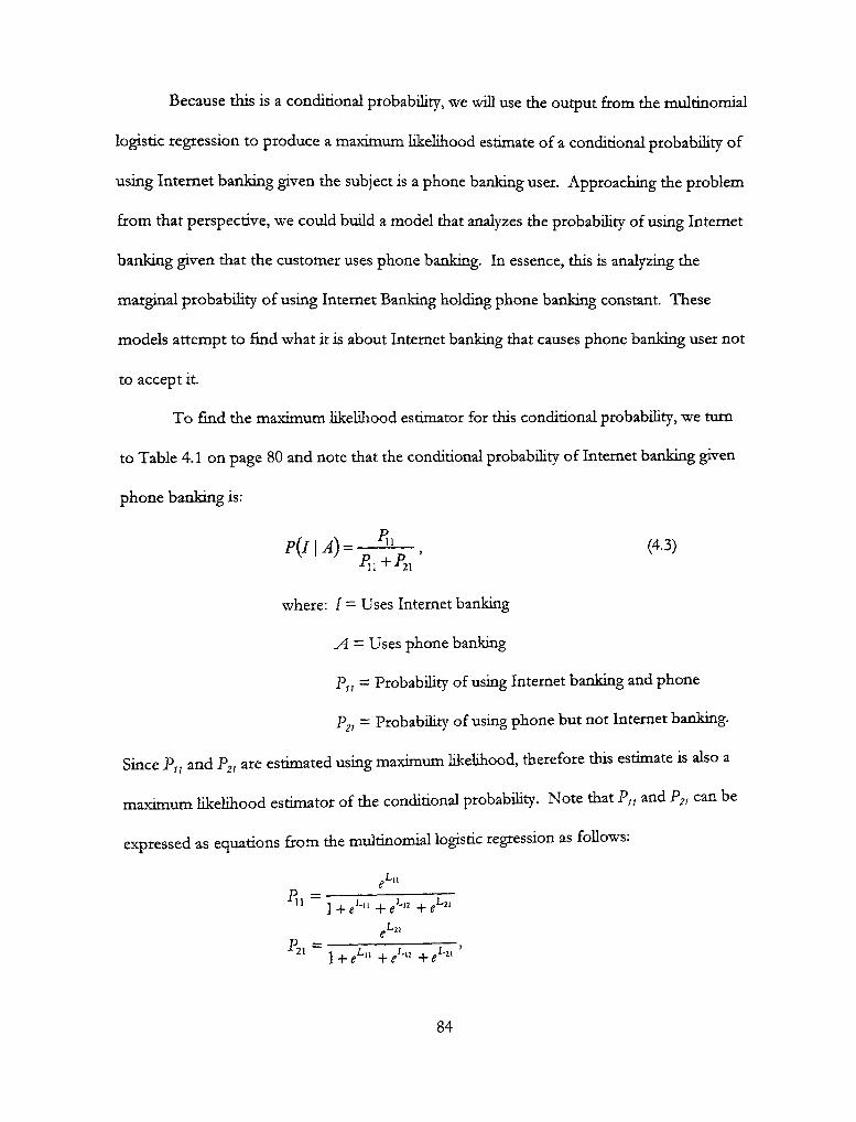
Because this is a conditional probabihty, we wUl use the output fiom the multinomial
logistic regression to produce a maximum hkehhood estimate of a conditional probabihty of
using Internet bankkig given the subject is a phone banking user. Approaching the problem
from that perspective, we could buUd a model that analyzes the probabihty of using Internet
banking given that the customer uses phone banking. In essence, this is analyzing the
marginal probabihty of using Internet Banking holding phone banking constant. These
models attempt to find what it is about Internet banking that causes phone banking user not
to accept it.
To find the maximum Hkehhood esthnator for this conditional probabUity, we tvim
to Table 4.1 on page 80 and note that the conditional probabUity of Internet banking given
phone banking is:
-Ml •^-'21
where: / = Uses Internet banking
A - Uses phone banking
P„ = ProbabUity of usmg Internet bankmg and phone
P2, = ProbabUity of usmg phone but not Internet bankkig.
Smce P„ and P^, are estimated using maximum Hkehhood, dierefore tiks estimate is also a
maxknum Hkehhood estimator of die conditional probabUity. Note tiiat P„ and P^, can be
expressed as equations fiom die multinomial logistic regression as foUows:
e ' p = — . —-
P„ = 2' I + / 1 . +^^12 + f ^ 2 ' '
84
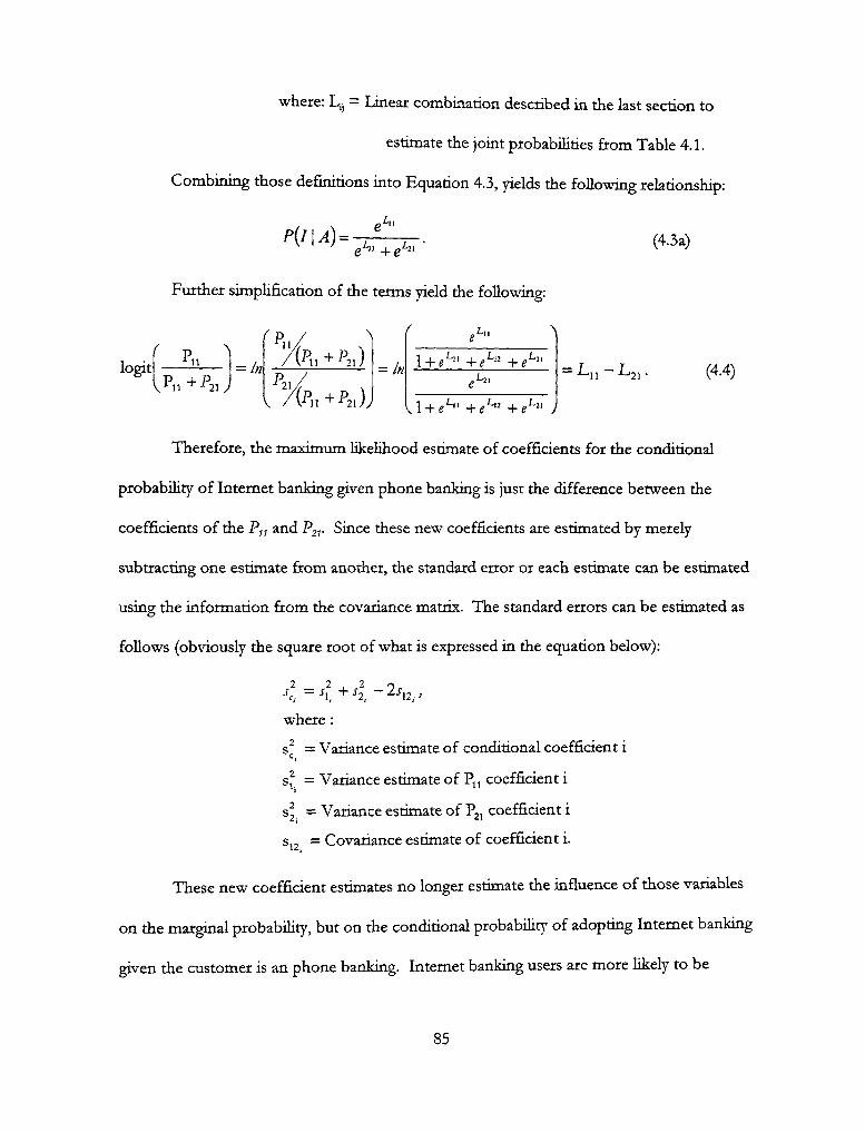
where: Li, = linear combination described in the last section to
estimate the joint probabUities fiom Table 4.1.
Combkikig those definitions into Equation 4.3, yields the foUowing relationship:
^( i )=:z^ e'"
Further sknphfication of the terms yield the foUowing:
(4.3a)
logit r p >
Pn+^21 = ln
(P / ^
^ 2 1
(^n+^2.).
= In
\
l + e'-" +6^''- -l-e^ '
U + e^" +e^" +e^" J
— i.^,] 1 21 (4.4)
Therefore, the maximum hkehhood estimate of coefficients for the conditional
probabihty of Internet banking given phone banking is just the difference between the
coefficients of the P,, and P^,. Since these new coefficients are estknated by merely
subtracting one estimate fiom another, the standard error or each estimate can be estimated
using the information fiom the covariance matrix. The standard errors can be estimated as
foUows (obviously the square root of what is expressed in the equation below):
j^_ — jj^ -r J2_ .^^12. J
where :
s = Variance estimate of conditional coefficient i
Si = Variance estimate of P„ coefficient i
Sj = Variance estimate of P2, coefficient i
s,2 = Covariance estknate of coefficient i.
These new coefficient estknates no longer estknate the kifluence of those variables
on the marginal probabUity, but on the conditional probabiht}' of adopting Internet bankkig
given the customer is an phone bankkig. Internet bankmg users are more hkely to be
85
computer Hterate, and own a computer, so we would expect titiat die education and kicome
variables to be sknUar to tiiose discussed in Section 4.1. The utihty gakied by those having
multiple accounts one would also expect to be positive. However, tiie coefficients on the
risk aversion variables (place holder for die risk prenuum) are not hypodiesized, and are the
focus of tills paper. If we let ^„ 4 , and ^3 be the coefficients of die dummy variable ki this
conditional probabihtj^ model of Internet given phone bankkig, then our most knportant
hypothesis for this analysis is:
H,^: ^,= ^^= ^j=0 Perceived risk is zero gokig fiom phone to Internet
banking.
Obviously, if only one risk measure is needed, only one ^ term needs to be used in
the above hypothesis.
In addition to the conditional probabihty of Internet given phone banking, it would
be interesting from an optkxuzation standpokit to examine the decision to adopt phone
given Internet banking Equation 3.6d. In essence, this would register any added risk
perceived by the customer going fiom Internet banking to phone banking. If we let tU], 2,
and tUj be the coefficients of the dummy variable in this conditional probabihty model of
phone given Internet banking, then our most important hypothesis for this analysis is:
Hjg: m,= CT,= crj=<?Perceived risk is zero going from Internet to phone
banking.
86
4.6 AUowkig Subjective ProbabUity to Vary
Up to this point, we have assumed that the subjective probabUity distribution is
identical across aU bank customers. As shown in Chapter 3, if the subjective probabUity
distributions can be changed, the risk premium wUl change, ceteris paribus. More importantiy,
if banks can do things to affect a reduction ki thek customers' subjective probabUity
distribution, reduckig the probabUity of adverse outcome, then the adoption rate wUl
mcrease.
We wiU now propose a test to see whether aU participants actuaUy have the same
subjective probabihty distribution. If customers do not have identical subjective probabihty
distributions, then banks may be able to affect them, and thereby affect thek customers' risk
premium. According to the equations developed in Chapter 3, the risk premium is a
function of subjective probabihty and risk aversion (see our Equation 3.6-as weU as Pratt's
Equations 5 and 7). For the most part, risk premium is merely the product of a measure of
subjective probabihty and risk aversion. Therefore, if a variable can be used to proxy for
subjective probabihty, interacting it with the risk aversion variable should proxy for the
consumer's risk premium.
Three variables used thus far as budget constraint variables could also lead
consumers to revise thek subjective probabUity distributions. Fkst, the older one is, the
more suspecting the consumer may be of the Internet in general. Therefore, the interaction
between age and risk should be negative. Second, the more education one has, the less
suspicious one might be of security on the Internet, having arguably more experience with
the medium. Therefore, higher levels of education should lead to higher adoption when
87
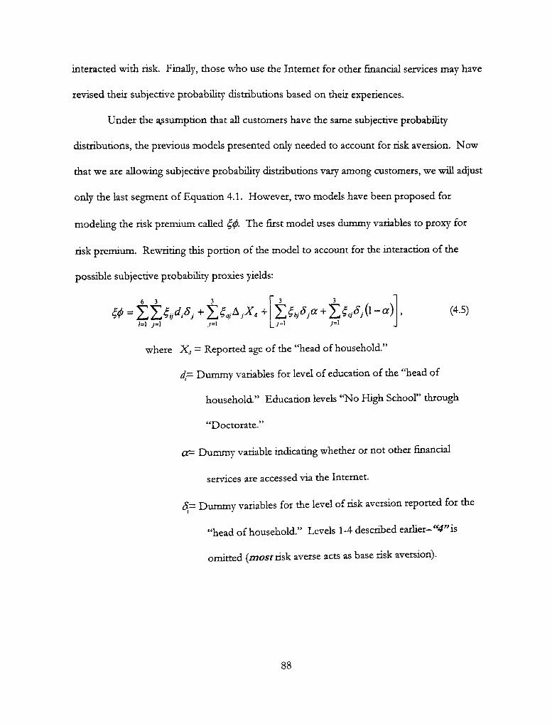
interacted with risk. FinaUy, tiiose who use tiie Internet for other financial services may have
revised thek subjective probabUity distributions based on thek experiences.
Under tiie assumption that aU customers have the same subjective probabUity
distributions, the previous models presented only needed to account for risk aversion. Now
that we are aUowkig subjective probabihty distributions vary among customers, we wUl adjust
only die last segment of Equation 4.1. However, two models have been proposed for
modeling the risk prenkum caUed ^^. The first model uses dummy variables to proxy for
risk premium. Rewriting this portion of the model to account for the interaction of the
possible subjective probabihty proxies yields:
6 3 3
/=1 7=1 7=1 7=1 J=I
(4.5)
where X^ = Reported age of the "head of household."
4.= Dummy variables for level of education of the "head of
household." Education levels "No High School" through
"Doctorate."
a= Dummy variable kidicating whether or not other financial
services are accessed via the Internet.
5- Dummy variables for the level of risk aversion reported for die
"head of household." Levels 1-4 described eariier-'<^"is
omitted {mostmk averse acts as base risk aversion).
88
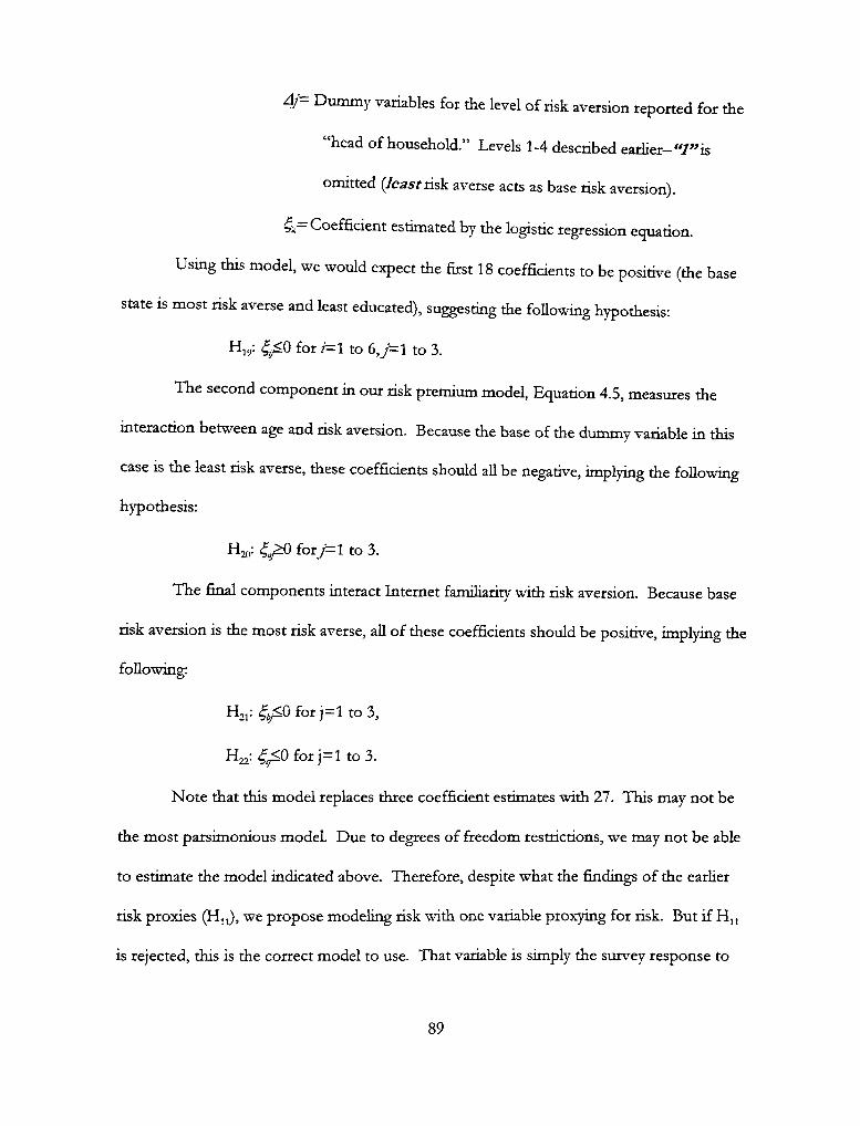
Aj- Dummy variables for die level of risk aversion reported for tiie
"head of household." Levels 1-4 described earher-"/' ' is
omitted (/easfrisk averse acts as base risk aversion).
4 = Coefficient estimated by die logistic regression equation.
Uskig tiks model, we would expect die first 18 coefficients to be positive (tiie base
state is most risk averse and least educated), suggesting die foUowkig hypotiiesis:
H,9: ^XO for z=l to 6,y=l to 3.
The second component ki our risk premium model, Equation 4.5, measures the
kiteraction between age and risk aversion. Because the base of die dummy variable in this
case is the least risk averse, tiiese coefficients should aU be negative, knplykig tiie foUowkig
hypothesis:
H20: ^>Q fory=l to 3.
The final components interact Internet famUiarity with risk aversion. Because base
risk aversion is the most risk averse, aU of these coefficients should be positive, knplykig the
foUowing:
H 3 , : ^ ^ 0 f o r j = l t o 3 ,
H22: 4;<0forj=l to3 .
Note that this model replaces three coefficient estimates with 27. This may not be
the most parsimonious model. Due to degrees of freedom restrictions, we may not be able
to estimate the model indicated above. Therefore, despite what the findings of the earher
risk proxies (H,,), we propose modeHng risk with one variable proxying for risk. But if H,,
is rejected, this is the correct model to use. That variable is simply the survey response to
89
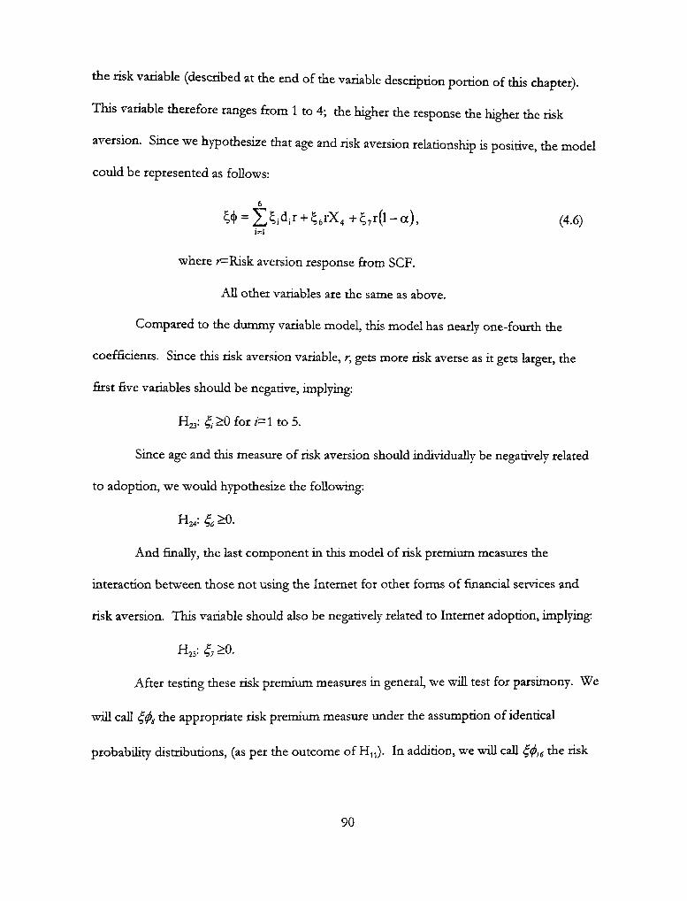
die risk variable (described at die end of die variable description portion of tiks chapter).
This variable dierefore ranges from 1 to 4; die higher tiie response tiie higher die risk
aversion. Skice we hypodiesize that age and risk aversion relationship is positive, die model
could be represented as foUows:
6
(t. = 2;^idir + , rX4+^ , r ( l - a ) , (4.6) i=I
where ;^Risk aversion response from SCF.
AU other variables are the same as above.
Compared to the dummy variable model, this model has neariy one-fourth the
coefficients. Since this risk aversion variable, r, gets more risk averse as it gets larger, the
first five variables should be negative, implying:
H23:4;.>0for?=l to 5.
Since age and this measure of risk aversion should individuaUy be negatively related
to adoption, we would hypothesize the foUowing:
H24:4^0.
And finaUy, the last cotnponent in this model of risk premium measures the
kiteraction between those not using the Internet for other forms of financial services and
risk aversion. This variable should also be negatively related to Internet adoption, implying:
H33:^,>0.
After testing these risk premium measures in general, we wiU test for parsimony. We
wiU caU £,^g the appropriate risk premium measure under the assumption of identical
probabUity distributions, (as per the outcome of H„). In addition, we wUl caU < ,g the risk
90

premium described by Equation 4.5 and ^^,7 the risk premium described by Equation 4.6.
To test to see whether customers have different subjective probabihties, either Equation 4.5
or Equation 4.6 should better describe the risk premium tiian Equation 4.1. To test this
hypothesis, we would test the foUowing (using a fiiU/reduced model fiamework):
If both Equations 4.5 and 4.6 add predictabihty to the model, we wiU need to test the
foUowing hypothesis as weU:
Hsa: ^'t>u - ^<PiT
If eitiier Equation 4.5 or 4.6 is more powerful than Equation 4.1, we wUl have shown
evidence that customers have different probabihty distributions based on education, age or
Internet commerce experience. In addition we may want to re-work the models described in
Sections 4.5 and 4.6. Since parsimony is important to being able to estimate that model,
non-significant variables may be trimmed before the final multinomial model is estimated.
Hypotheses Hjy through H23 wUl be repeated on the marginal model fiom Section 4.5 to test
the role of both risk aversion and probabUity in die margkial adoption decisions. Aldiough
these tests may not be run if it is deemed that the model makes it hard to interpret the
results.
91
CHAPTER 5
EMPIRICAL RESULTS
This chapter empiricaUy tests the models and hypotheses set forth ki Chapter 4. To
begin with, we present descriptive statistics of aU variables used in the models. FoUowkig
the descriptive statistics section the models are tested as set forth ki Chapter 4. For
convenience, the section numbers correspond to those of the last chapter. In other words,
Section 5.2 presents empirical results of the base models presented in Section 4.2. Section
5.3 contains empirical results of tests concerning the functional forms. Section 5.4 presents
findings of the multinomial model, which leads to the modeHng of marginal propensity to
adopt (conditional probabUities) in Section 5.5. And finaUy, we present empirical results
from testing for varying subjective probabihties in 5.6.
5.1 Descriptive Statistics
We begin analyzing the data by presenting the descriptive statistics for the variables
used in the models described earher. Where appropriate, we use univariate statistical
techrkques to detect differences ki responses by adoption of different remote access bankkig
technologies.
We wUl consider the proposed response variables first. Table 5.1 contams cross-
tabulations of Internet and phone bankkig fiom die 1998 SCF. The figures represent die
weighted responses as described ki Section 4.1. Of tiie nearly 4,305 interviewed, our sample
(after weighting for the general population) kicludes 4,016 bank customers. Of tiiose, 163
92

used Internet banking, 1,193 used voice phone bankkig, 902 used touchtone phone bankmg,
and 1,606 used at least one of those forms of phone banking.
Table 5.1 - Internet and Phone-Banking Utilization
Internet Banldng No Internet Bankkig Total Panel A - Cross-tabulation of Internet Bankkig and Phone Banking (Voice)
Phone Bankkig (Voice) 76 1117 1193
No Phone Banking (Voice) 87 2 736 2 823
163 3,853 4,016
Panel B - Cross-tabulation of Internet Bankmg and Phone Banking (Touchtone)
Phone Bankkig (Touchtone) 80 822 902
No Phone Bankkig (Touchtone) 83 3,030 3,113
163 3,852 4,015
Panel C - Cross-tabulation of Internet Banking and Phone Banking (Any)
Phone Bankkig (Any) 106 1,500 1,606
No Phone Bankkig (Any) 57 2,353 2,410
163 3,853 4,016
It is interesting to note that of those using Internet banking roughly fifty percent use
touchtone banking (the least user friendly, but the most computerized). Voice phone
banking is used by fewer than half of the Internet banking users. But neariy two-thkds of aU
Internet bankkig customers use some form of phone banking, demonstrating a demand for
remote or after-hours banking.
The predictor variables wUl be presented according to thek theoretical construct
beginning with the variables prox}'ing for utiHty. Panel A of Table 5.2 contains the
descriptive statistics for Number of Checkkig Accounts {#Checks), Number of Savkigs
93

Accounts {#Savings), and Liquid Account Balances (Liquid). Since the Liquid Account
Balance variable is so skewed, the natural log of that variable plus 71 also is taken
{ln(LJqziid+71J). The last variable adds 71 before taking the natural log, so that the natural
log exists for aU observations.
Note that aU of these variables are skewed. The fkst two variables appear skewed
because they have a lower bound, zero, but no upper bound. In addition, the mean is very
close to the lower bound. Therefore, there is no symmetrical distribution around the mean.
It is important to note that the variable whose mean is closest to zero also has the highest
skewness coefficient.
The reason that the Liquid Account Balance variable is so skewed is different There
are a few very large observations. These observations are correlated with the income
variable to be discussed later.'^ Because of the extreme skewness in this variable, the natural
log of the variable wUl be used in aU of the analysis that foUows, even though that variable is
more closely correlated with natural log of income, which is also a predictor variable.
Note that the smaUest observation for Liquid Account Balances is - 7 1 . This entke
negative amount is ki the checkkig account (and the household has no savings accounts).
Apparendy this observation is an overdraft balance.
Panel B reports the outcome of hypodiesis tests of equahty of means among tiiose
adopting or not adopting the different remote access technologies:
^ 0 " Hrcmotc ~ M'conventional
•' The estimated correlation coefficient between Liquid Account Balances and Income is 0.194, between Liquid Account Balances and natural log of Income is 0.164, and between natural log of Liquid Account Balances and natural log of Income is 0.499. M of diese estimates are statistically different from zero at die 0.01 level.
94
Positive (negative) test statistics represent larger (smaUer) sample means for die remote
bankkig sub-sample tiian for tiie conventional bankmg sub-sample. This testis run because
good predictor variables should differ on average by die response variable. In panel B, it is
knportant to note tiie degrees of freedom. When die degrees of freedom are not 4,013, then
die variances were found to differ (at die 0.05 level). Many of die tests conducted on tiiese
variables showed a difference m variance. In die case of the first two variables, the reason
for difference in variance is die same as die reason for skewness. Skice diere is a firm lower
bound, the variance should be different if the mean is different.
In the case of the Liquid Account Balance variable (JJquid), sometimes there were
different variances, and sometimes not, depending on where the outhers feU. It is interesting
to note that even when the natural log was taken {ln(Liquid+71J), gteatiy reducing the
skewness, half of the tests stiU showed difference in variance, due to the outiier problem.
Of the variables in Table 5.2, both the Number of Checking Accounts and the
natural log of Liquid Accovmt Balances appear to be exceUent determinants of remote
banking adoption. Number of Savings accounts is an exceUent determinant of phone-
banking, and is a good determinant of Internet banking, but wiU depend on whether or not
there is some correlation between number of checkkig and savings accovmts. Liquid
Account Balances (not the natural log) appears to be a mediocre predictor variable. AU signs
are consistent with our expectations except for the Liquid Asset Accoimt Balances for
Touchtone.
95
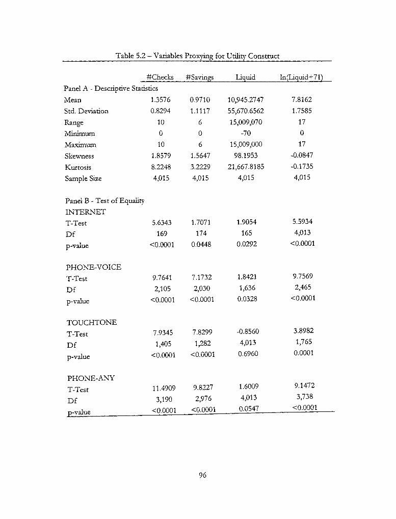
Table 5.2 - Variables Proxying for UtiHty Construct
#Checks
Panel A - Descriptive Statistics
Mean
Std, Deviation
Range
Minimum
Maximum
Skewness
Kurtosis
Sample Size
Panel B - Test of Equahty
INTERNET
T-Test
Df
p-value
PHONE-VOICE
T-Test
Df
p-value
TOUCHTONE
T-Test
Df p-value
PHONE-ANY
T-Test
Df p-value
1.3576
0.8294
10
0
10
1.8579
8.2248
4,015
5.6343
169
<0.0001
9.7641
2,105
<0.0001
7.9345
1,405
<0.0001
11.4909
3,190
<0.0001
#Savings
0.9710
1.1117
6
0
6
1.5647
3.2229
4,015
1.7071
174
0.0448
7.1732
2,030
<0.0001
7.8299
1,282
<0.0001
9.8227
2,976
O.OOOl
Liquid
10,945.2747
55,670.6562
15,009,070
-70
15,009,000
98.1953
21,667.8185
4,015
1.9054
165
0.0292
1.8421
1,636
0.0328
-0.8560
4,013
0.6960
1.6009
4,013
0.0547
lnCLiquid-^71)
7.8162
1.7585
17
0
17
-0.0847
-0.1735
4,015
5.5934
4,013
<0.0001
9.7569
2,465
<0.0001
3.8982
1,765
0.0001
9.1472
3,738
<0.0001
96
Tlie variables proxykig for die budget constrakit wUl be presented ki die next set of
tables. Fkst tiie quantitative variables are presented ki Table 5.3, tiien education wUl be
presented ki Table 5.4, and finaUy famUiarity witii electronic financial services wUl be
presented in Table 5.5.
In Chapter 4, we proposed bodi die age of die head of household (Age) and die
natural log of income (InflncomeJ) as budget constrakit variables. These variables are
presented ki Table 5.3. The format is identical to Table 5.2. It presents tiie descriptive
statistics first, tiien tests the hypothesis of equahty of means. Unlike the variables presented
before, neitiier of tiiese variables have a problem witii skewness, altiiough the kicome
measure stUl has a significant amount of kurtosis. It is however knportant to note that the
natural log of income has a somewhat smaUer sample size. The survey does not disclose the
negative kicomes reported, just that they were negative. For our purposes, we have dropped
these observations.
The average age of a head of household is 49 years old, with the oldest in the sample
95 years old and the youngest oiUy 17.
The kicome variable is a httie more difficult to interpret because it is the natviral log
of income. The average natural log of income is associated with an income of around
$34,000 (although this is not the average income by any means). The highest income in the
sample is $176 milhon. The income reported was for 1997, and does not necessarUy reflect
ongoing income. Because of the expected extreme skew caused by several outhers, the
natural log of this variable was taken from the start
97
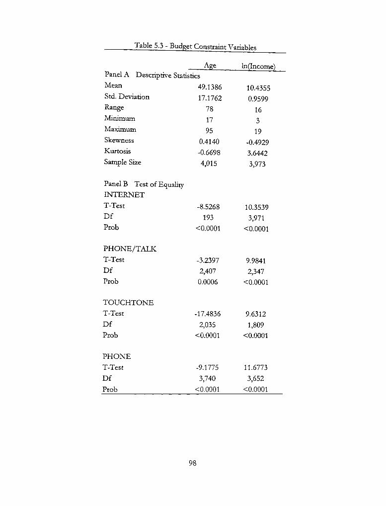
Table 5.3 - Budget Constrakit Variables
Age hi(Income) Panel A Descriptive Statistics
Mea" 49.1386 10.4355 Std. Deviation 17.1762 0.9599
Range jg 16
Minimum \j 3
Maximum 95 ^9
Skewness 0.4140 -0.4929
Kurtosis -0.6698 3.6442
Sample Size 4^015 3,973
Panel B Test of Equahty
INTERNET
T-Test
Df
Prob
PHONE/TALK
T-Test
Df
Prob
TOUCHTONE
T-Test
Df
Prob
PHONE
T-Test
Df
Prob
-8.5268
193
<0.0001
-3.2397
2,407
0.0006
-17.4836
2,035
<0.0001
-9.1775
3,740
<0.0001
10.3539
3,971
<0.0001
9.9841
2,347
<0.0001
9.6312
1,809
<0.0001
11.6773
3,652
<0.0001
98
In panel B of Table 5.2 we find the tests of equahty of means. It is interesting that
the means are significantiy different from zero, and that the signs are consistent with our
expectations. In other words, these variables appear to be good predictors of remote
banking adoption. Education was expected to famUiarize customers with computer
technology, and thereby reduce tiiek marginal adoption costs. Panel A of Table 5.4 shows
the overaU frequency of occurrence of different levels of education. These education levels
represent the highest level of education attained by the head of household. The levels are
not fiikshed Ikgh school (NHS), high school (HS), some coUege (SC), bachelor's degree
(BA), masters degree (MA) and doctorate (DR). The most common education level was
High School, foUowed by Some CoUege. The median education level was Some CoUege.
Panels B and C convey much the same information in different formats. Panel B
shows the raw cross-tabulations. Panel C restates Panel B showkig the proportion of remote
banking type in each education category. Panel C is easier to interpret however. Note that
the proportion of Internet banking adopters with Some CoUege is approximately the same as
the overaU sample; as is the proportion of non-Internet bankkig adopters. However, as one
moves away from the median education of the sample, the education proportions by
Internet banking adoption diverge. The phone-bankmg adoption decisions seem to be
based on education as weU, but the pattern does not seem by symmetrical around die Some
College response as it does in Internet banking.
99
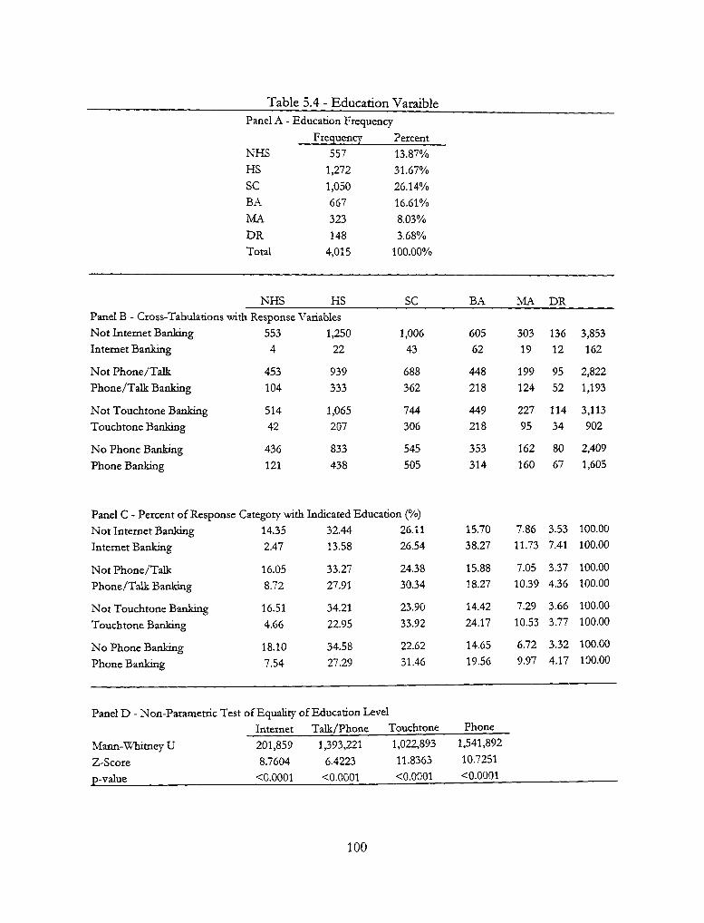
Table 5.4 - Education Varaible Panel A -
NHS
HS
SC
BA
MA
DR
Total
NHS
Education Frequency
Frequency
557
1,272
1,050
657
323
148
4,015
HS
Panel B - Cross-Tabulations with Response Variables
Not Internet Banking
Internet Banking
Not Phone/Talk
Phone/Talk Banking
Not Touchtone Banking
Touchtone Banking
N o Phone Banking
Phone Banking
553
4
453
104
514
42
436
121
1,250
22
939
333
1,065
207
833
438
Percent
13.87%
31.67%
26.14%
16.61%
8.03%
3.68%
100.00%
SC
1,006
43
688
362
744
306
545
505
BA
605
62
448
218
449
218
353
314
MA
303
19
199
124
227
95
162
160
DR
136
12
95
52
114
34
80
67
3,853
162
2,822
1,193
3,113
902
2,409
1,605
Panel C - Percent of Response Category with Indicated Education (%) Not Internet Banking
Internet Banking
Not Phone/Talk
Phone/Talk Banking
Not Touchtone Banking
Touchtone Banking
No Phone Banldng
Phone Banking
14.35
2.47
16.05
8.72
16.51
4.66
18.10
7.54
Panel D - Non-Parametric Test of Equality
Mann-Whitney U
Z-Score
p-value
Internet
201,859
8.7604
<0.0001
32.44
13.58
33.27
27,91
34.21
22.95
34.58
27.29
26.11
26.54
24.38
30.34
23.90
33.92
22.62
31.46
of Education Level
Talk/Phone
1,393,221
6.4223
<0.0G01
Touchtone
1,022,893
11.8363
<0.0001
15.70
38.27
15.88
18.27
14.42
24.17
14.65
19.56
Phone
1,541,892
10.7251
<0.0001
7.86
11.73
7.05
10.39
7.29
10.53
6.72
9.97
3.53
7.41
3.37
4.36
3.66
3.77
3.32
4.17
100.00
100.00
100.00
100.00
100.00
100.00
100.00
100.00
100
Because education level is an ordkial measure, we test to see ktiie mid-pomts (T]) of
die distributions are die same uskig a Mann-Whitoey test:
0- Itcmote " 'Iconventional ~ ^ -
Panel D shows die results of that test Note tiiat aU tests signs are consistent witii
tiie tiieory and are significant at any reasonable level. Education appears to be a good
predictor of remote bankkig adoption.
The last variable proxykig for budget constrakit was die customer's famUiarity witii
financial services via tiie Internet This variable kidicated whetiier tiie household accessed
any odier financial services via die Internet Panel A of Table 5.5 shows cross-tabulations of
otiier financial services via die Internet witii tiie response variables ki tiks research. Only
Internet bankkig is expected to be dependent on tins variable; the other variables were added
for completeness.
If this variable is a good predictor of the response variables ki a logit framework,
then the rows and columns ki the cross-tabvUations should be statisticaUy dependent (i.e.,
knowing that a subject uses the Internet to manage another financial type account changes
the probabihty that they use Internet banking). A chi-square test is run to test for
dependence, and is reported in panel B of Table 5.5. It is interesting that in aU cases
dependence between famiHarity and response variables is significant That would mean that
knowing that someone used the Internet to interact with a financial services provider would
cause one to revise one's estimates of the probabihty that they wovUd use phone-banking.
Although the theory does not predict that dkecdy, the fact that many of the other variables
discussed thus far have been good predictors of both Internet and phone-banking suggest
101
that we may be pickkig up the other concepts in this variable; only the logistic regression wiU
teU.
FinaUy, panel C reports the financial service provider used by the customers ki the
survey. The most popvUar Internet financial service reported in the SCF is Internet banking,
foUowed by security brokerages or mumal funds(Brokerage). Finance/Loan companies
(Finance Company) were a respectable, but distant thkd. The other category had too many
to hst, including insurance companies and student loans.
The final variable used in die logistic regression models is the risk aversion measure.
As explained earher, it is not yet clear how this variable wUl be treated. It could be treated as
a quantitative variable, or it could be treated as a categorical variable. Table 5.6 presents
descriptive statistics as if the risk variable were a quantitative variable, in the same format as
presented ki Tables 5.2 and 5.3. Panel B tests the equahty of means as ki Tables 5.2 and 5.3.
102
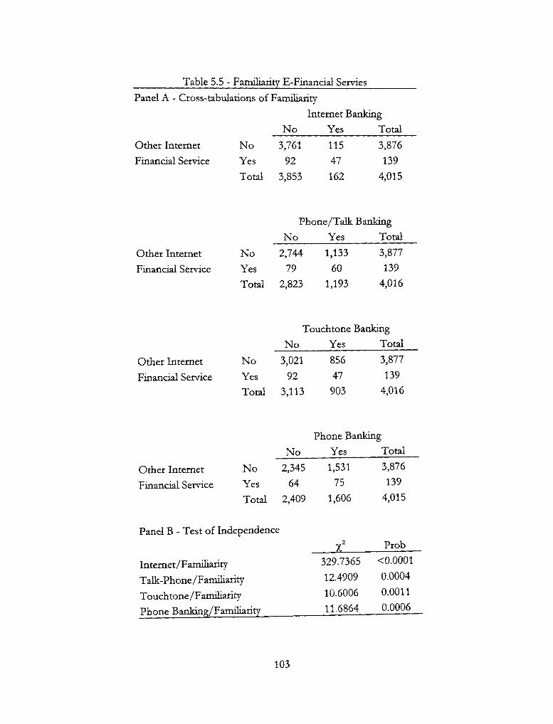
Table 5.5 - FamUiarity E-Financial Servies
Panel A - Cross-tabulations of FamUiarity
Internet Banking
No Yes Total
Other Internet
Financial Service
No
Yes
Total
3,761
92
3,853
115
47
162
3,876
139
4,015
Phone/Talk Banking
No Yes Total
Other Internet
Financial Service
No
Yes
Total
2,744
79
2,823
1,133
60
1,193
3,877
139
4,016
Touchtone Banking
No Yes Total
Other Internet
Financial Service
Other Internet
Financial Service
No
Yes
Total
No
Yes
Total
3,021
92
3,113
No
2,345
64
2,409
856 3,877
47 139
903 4,016
Phone Banking
Yes Total
1,531 3,876
75 139
1,606 4,015
Panel B - Test of Independence
Internet/ FamUiarity
Talk-Phone/FamUiarity
Touchtone / FamUiarity
Phone Bankkig/FamUiarity
Prob
329.7365 <0.0001
12.4909 0.0004
10.6006 0.0011
11.6864 0.0006
103
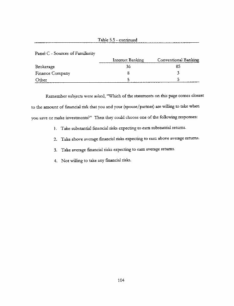
Table 5.5 - continued
Panel C - Sources of FamiHarity
Internet Banking Conventional Banking
Brokerage 36 85
Finance Company 8 3
Otiier 5 5
Remember subjects were asked, "Which of the statements on tiks page comes closest
to the amount of financial risk that you and your (spouse/partner) are wUhng to take when
you save or make kivestments?" Then they could choose one of the foUowkig responses:
1. Take substantial financial risks expecting to earn substantial returns.
2. Take above average financial risks expectkig to earn above average returns.
3. Take average fkianckil risks expecting to earn average returns.
4. Not wUling to take any financial risks.
104
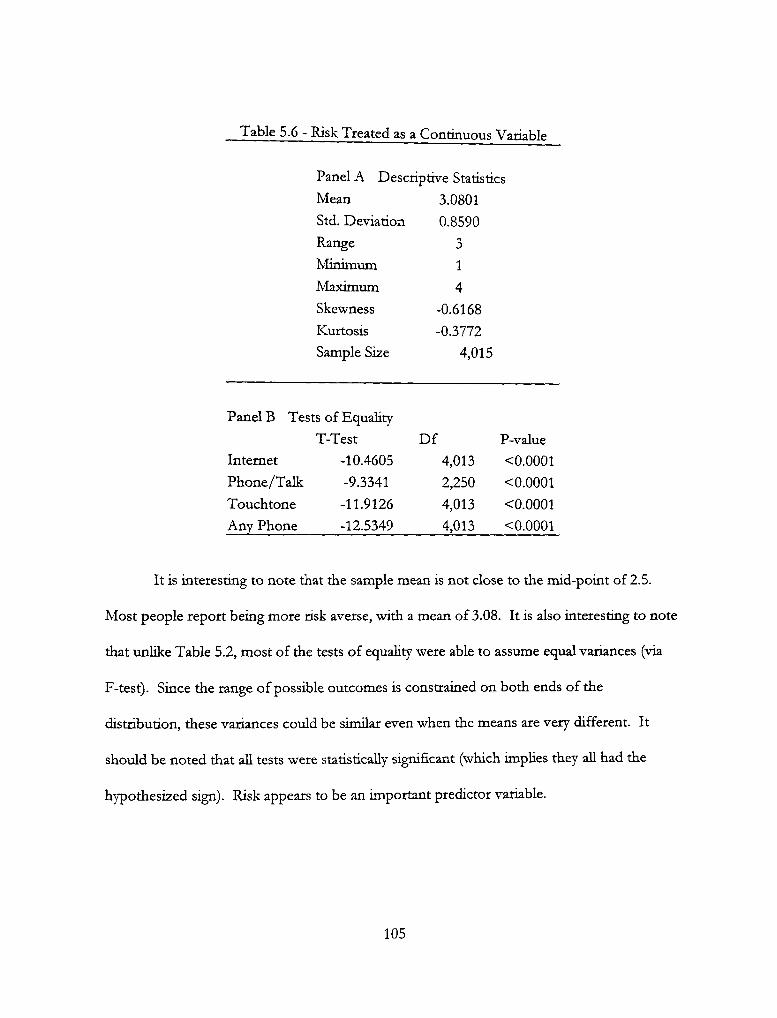
Table 5.6 - Risk Treated as a Continuous Variable
Panel A Descriptive Statistics
Mean
Std. Deviation
Range
Minimum
Maximum
Skewness
Kurtosis
Sample Size
3.0801
0.8590
3
1
4
-0.6168
-0.3772
4,015
Panel B Tests of Equahty
T-Test
Internet -10.4605
Phone/TaUc -9.3341
Touchtone -11.9126
Any Phone -12.5349
4,013
2,250
4,013
4,013
P-value
<0.0001
<0.0001
<0.0001
<0.0001
It is interesting to note that the sample mean is not close to the mid-point of 2.5.
Most people report being more risk averse, with a mean of 3.08. It is also interesting to note
that unlike Table 5.2, most of the tests of equahty were able to assume equal variances (via
F-test). Since the range of possible outcomes is constrained on both ends of the
distribution, these variances could be sknUar even when the means are very different. It
should be noted that aU tests were statisticaUy significant (which impHes they aU had the
hypothesized sign). Risk appears to be an knportant predictor variable.
105

Table 5.7 presents risk as a categorical variable. Panel A shows the overaU frequency
of responses (weighted consistent with the overaU population of the United States). The
median response is 3 (close to the mean in Table 5.6).
Panel B presents proportions of aU response variable outcomes that represent levels
of risk aversion. Again the Internet banking distribution is easy to interpret Those adoptkig
Internet banking report less risk aversion in general. AU risk aversion responses are equaUy
important in explaining the difference in Internet banking adoption.
For aU types of phone banking, nsk aversion responses for two and four appear to
be better predictors (there is a bigger difference between percentages of given phone/non-
phone banking than risk levels one and three). That may mean that this variable wiU work
weU as a continuous variable for Internet banking, but not for phone-banking.
Even as a categorical variable, risk aversion is theoreticaUy ordinal. Therefore, a
Mann-Whitney test can be performed on it as foUows:
•^•0' Iremote " Iconventiona]
In this hypothesis, the r| is the mid-pokit of each distribution. The results of these
tests are found ki panel C. The tiieory suggests that the lower the risk aversion, the higher
the adoption probabihty. Therefore, aU of tiie test statistics should be negative, which tiiey
are.
106
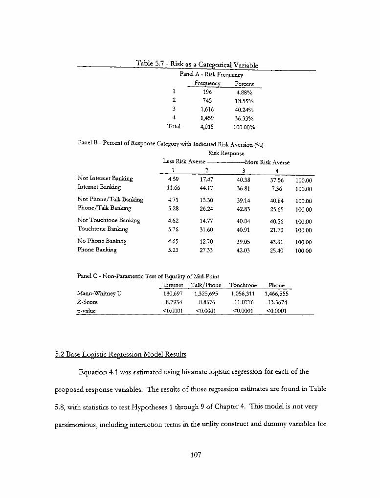
Table 5.7 - Risk as a Categorical Variable Panel A - Risk Frequency
Frequency
1 196
2 745
3 1,616
4 1,459
Total 4,015
Percent
4.88%
18.55%
40.24%
36.33%
100.00%
Panel B - Percent of Response Category witii Indicated Risk Aversion (%)
Risk Response
Not Internet Banking
Internet Banking
Not Phone/Talk Banking
Phone/Talk Banking
Not Touchtone Banking
Touchtone Banking
No Phone Banking
Phone Banking
Panel C - Non-Parametric Test of Equality of Mid-Point
Internet Talk/Phone Touchtone Phone
1
4.59
11.66
4.71
5.28
4.62
5.76
4.65
5.23
2
17.47
44.17
15.30
26.24
14.77
31.60
12.70
27.33
3
40.38
36.81
39.14
42.83
40.04
40.91
39.05
42.03
xvjaii. .f\ verse 4
37.56
7.36
40.84
25.65
40.56
21.73
43.61
25.40
100.00
100.00
100.00
100.00
100.00
100.00
100.00
100.00
Mann-WHtneyU 180,697 1,325,695 1,056,311 1,466,555
Z-Score -8.7934 -8.8676 -11.0776 -13.3674
p-value <0.0001 <0.0001 <0.0001 <0.0001
5.2 Base Logistic Regression Model Results
Equation 4.1 was estimated using bivariate logistic regression for each of the
proposed response variables. The results of those regression estimates are found in Table
5.8, with statistics to test Hypotiieses 1 through 9 of Chapter 4. This model is not very
parsimonious, including interaction terms in the utihty construct and dummy variables for
107
each risk aversion response. However, it is a good startkig pokit for our analysis. Panel A
shows coefficient estimates and Wald test statistics ki parentheses. Panel B shows overaU
model fit statistics. The chi-square figure ki Panel B tests Hypotheses 1 from Chapter 4.
Note that Hj'potheses 1 (for aU response variables) is rejected; the model appears to have
some predictive value.
Hypotheses 2 relate to the importance of the number of checking accounts to the
adoption decision of different remote access technologies (interacting with risk). In the case
of Internet banking, it appears that number of checking accovints only matter k the risk
aversion response is 3. Tiks variable (interacting with risk) is a better predictor in the case of
aU definitions of phone-banking. It should, however, be noted that some of these
coefficients have the wrong sign (and would be significant if we had hypothesized that they
were equal to zero). In this and other cases where risk aversion response 3 is significant, one
must remember that response 3 occurs more often than the others, therefore it is easier to
find significance.
The coefficients of number of savkigs accounts corresponds to Hypothesis 3. This
is not generaUy as good a measure as is die number of checkkig accounts. It too works
better with phone-bankkig. And agaki, at least one coefficient has die wrong sign.
Hypotheses 4 relate to the hquid account balance variables. This variable could be
positive or negative. And agaki, only for risk aversion level 3 is tiks kiteraction variable
significant. The sign depends on die remote access metiiod.
Hypotiieses 5 relate to tiie age variable, tiie first of tiie budget constrakit variables.
This coefficient is negative and statisticaUy sigmficant for aU but voke phone bankmg,
consistent widi die stated hypotiieses. As stated m Section 4.1, age is a proxy for computer
108

and Internet trakiing. The younger tiie subject, tiie more hkely they are to have received
formal computer/Internet trainkig ki school. Even touchtone bankkig is closely related to
computers, skice you use die phone to interface widi tiie bank's computer; knplying that
those with a computer background would be better trained to understand i t Voice phone
banldng is the oldest technology of the group, and should be understood by roughly aU
customers.
Hypothesis 6 relates to the affect of income on remote banking technologies. We
wovUd expect those with higher incomes to be more likely to have aheady invested in
computer technology, making Internet banking less expensive. It may not affect the other
remote banking channels. In aU but the touchtone phone banking model, income is
significant and is positive. Touchtone banking is significantiy negative, su^esting that
customers with lower incomes are more Hkely to adopt it. It is unclear why this variable is
positive for other forms of phone banking.
Education was expected to affect computer Hteracy (and thereby Internet banking)
and possibly touchtone phone banking. As discussed in Section 4.1, education was expected
to train people in computer Hteracy and Internet usage. However, as education shifts from
the general to speciahzation (as it does in graduate school), the benefit may not be as
knportant. Bachelor's degree was, therefore, treated as the base. AU lower levels of
education are significant in the Internet model. It is kiteresting to note that had we not
proposed a one-taUed test, the higher levels would also be significant. Voice phone banking
model only found one variable to be significant, and has die wrong sign (which flows
through to aU phone banking types).
109

FamiHarity indicates whether or not the household uses another form of Internet
financial services. We found in the descriptive statistics that this variable tj'picaUy indicates
that the customer uses Internet brokerage or investment services. Hypothesis 8 relates to
the effect of this variable on remote banking adoption. Only Internet banking was
hypothesized to be affected by this variable. This variable is only significant in the Internet
model.
The risk aversion variables were expected to affect aU types of remote banking. AU
models show some sigikficance in at least one risk aversion variable. But the phone banking
models do not show aU variables sigikficant as the Internet bankkig estimates do. These
results are roughly consistent with Hypothesis 9.
110
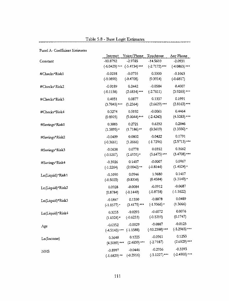
Table 5.8 - Base Logit Estimates
Panel A- Coefficient Estimates
Constant
#Checks*Riskl
#Checks*Risk2
#Checks*Risk3
#Checks*Risk4
#Savings*Riskl
#Savings*Risk2
#Savings*Risk3
#Savings*Risk4
Ln(Liquid)*Riskl
Ln(Liquid)*Risk2
Ln(Liquid)*Risk3
Ln(Liquid)*Risk4
Age
Ln (Income)
NHS
Internet
-10.8792
(-6.0429) ***
-0.0218
(-0.0890)
-0.0189
(-0.1158)
0.4951
(3.7045)***
0.3274
(0.8925)
0.3883
(1.5895) *
-0.0409
(-0.3661)
-0.0638
(-0.5207)
-0.3926
(-1.2264)
-0.1090
(-0.5025)
0.0928
(0,8784)
-0.1847
(-1.8577)*
0.3255
(1.6324)*
-0.0352
(-4.5143)**"
0.5648
(4.5089) **'
-0.8997
(-1.6820)**
Voice/Phone
-2.9785
(-5.4134)***
-0,0755
(-0.4708)
0.2442
(2.6834)***
0.0877
(1.2364)
0.5192
(5.0044)***
0.2721
(1.7186)**
0.0802
(1.2666)
0.0778
(1,6131)*
0,1407
(2.0042)**
0,0946
(0,8338)
-0,0084
(-0,1440)
0,1350
(3.4175)***
-0.0295
(-0.6233)
-0.0029
' (-1.1588)
0.1225
" (2.4839) ***
-0.0446
(-0.2916)
Touchtone
-14,5610
(-2.7172)***
0.5300
(0.3014)
-0,0584
(-2,7611)
0.1337
(2.6629) ***
-0,0061
(-2,4243)
0,6232
(0,5619)
-0,0422
(-1.7296)
0.0352
(3.6475)***
-0,0007
(-0,8144)
1,9680
(0.4584)
-0.0912
(-0.8738)
-0,8878
(-1.9366)*
-0.6072
(-0,1219)
-0,0887
(-10,2300)***
-0.0961
(-2,7187)
-0,2956
(-5,1227)***
Any Phone
-2,0931
(-4,0863) ***
-0,1063
(-0,6817)
0,4007
(3,9265)***
0,1991
(2,8163)***
0,4464
(4,5283) ***
0.2046
(1,3330)*
0,1791
(2,5713) ***
0,1662
(3,4708) ***
0,0967
(1,4524)*
0,1417
(1,3149)*
-0,0687
(-1,1622)
0.0489
(1.3066)
0.0076
(0.1747)
-0.0125
(-5.2965) ***
0.1253
(2.6929)***
-0.3593
(-2,4900) *»•
111
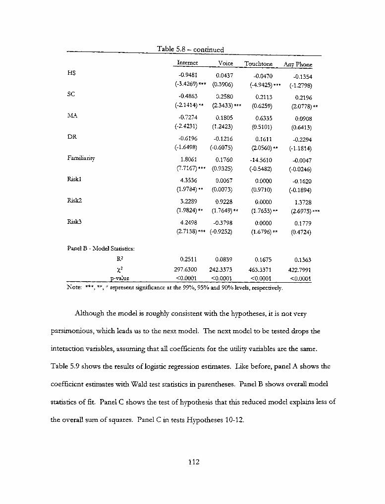
Table 5,8 - continued
HS
SC
MA
DR
Familiarity
Riskl
Risk2
Risk3
Panel B - Model Statistics:
R2
y} p-value
Internet
-0,9481
(-3,4269)***
-0,4863
(-2,1414)**
-0,7274
(-2.4231)
-0,6196
(-1,6498)
1,8061
(7,7167)***
4,3536
(1,9784)**
3,2289
(1,9824)**
4.2498
(2.7138)***
0,2511
297,6300
<0,0001
Voice
0,0437
(0,3906)
0,2580
(2.3433) ***
0,1805
(1,2423)
-0,1216
(-0,6075)
0,1760
(0,9325)
0,0067
(0,0073)
0,9228
(1,7649)**
-0,3798
(-0,9252)
0,0839
242,3373
<0,0001
Touchtone
-0,0470
(-4.9425)***
0.2113
(0.6259)
0.6335
(0,5101)
0,1611
(2,0560)**
-14,5610
(-0,5482)
0,0000
(0,9710)
0,0000
(1,7653)**
0,0000
(1,6796) **
0,1675
463,3371
<0,0001
Any Phone
-0.1354
(-1,2798)
0,2196
(2,0778)**
0,0908
(0,6413)
-0,2294
(-1,1814)
-0.0047
(-0.0246)
-0.1620
(-0,1894)
1,3728
(2,6975)***
0,1779
(0,4724)
0,1363
422,7991
<0,0001
Note: ***, **, * represent significance at the 99%, 95% and 90% levels, respectively.
Although the model is roughly consistent with the hypotheses, it is not very
parsimonious, which leads us to the next model. The next model to be tested drops the
interaction variables, assuming that aU coefficients for the utiHty variables are the same.
Table 5.9 shows the resvJts of logistic regression estimates. Like before, panel A shows the
coefficient estimates with Wald test statistics in parentheses. Panel B shows overaU model
statistics of fit. Panel C shows the test of hj'pothesis that this reduced model explains less of
the overaU sum of squares. Panel C in tests Hypotheses 10-12.
112
The results of tiie test of Hypotiieses 10-12 sknultaneously is kiteresting. In aU but
tiie voice phone banking model, tiiere is no difference ki the predictive power of this more
parsknonious model tiian tiie base model at die 5% significance level. Because tiks model is
more parsknonious and is generaUy no different from the much larger base model, this
model wiU be treated as die new base model.
In addition to the model bekig much more parsimomous, the coefficient estimates
are more consistent with the hypotheses and the theoretical model. The number of checkkig
accounts is a significant predictor in aU models. The number of savings accounts is a
significant predictor of phone bankkig adoption. Amount of Hqvud asset balances is not a
good predictor except in the case of voice phone banking, and there the relationship is
positive (i.e., the higher tiie Hquid asset balance the higher the probabihty of adoption).
Age acts as hypothesized; the younger the head of household, the more likely they
have adopted a remote banking solution. Education works roughly the way it was expected;
although those with masters appear to be less hkely to adopt Internet banking, counter to the
theory. Even with phone banking education seems to matter. And famiHarity with Internet
financial sei-vices only appear to matter for Internet banking.
AU risk aversion variables act as hypothesized, aU are positive and significant,
although the significance of the least risk averse variable is margkial ki the case of phone
banking.
As stated before, this model is both more parsknonious and more consistent with
our theory and hypotheses. To test for more parsknony, we try coUapsing die risk aversion
variables kito one variable, sknply the same number given by subjects ki the SCF (1, 2, 3 or
4), which increases the degrees of freedom by two.
113
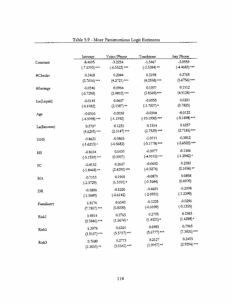
Table 5.9 - More Parsimoiuous Logit Estimates
Constant
#Checks
#Savings
Ln (Liquid)
Age
Ln (Income)
NHS
HS
SC
MA
DR
Familiarity
Riskl
Risk2
Risk3
Internet
-8.4695
(-7.1395)***
0.2468
(2.7616)***
-0.0546
(-0,7298)
-0,0141
(-0,1982)
-0,0355
(-4,5998)***
0,5707
(4,6295)***
-0,8621
(-1.6213)*
-0.8654
(-3.1559)***
-0.4132
(-1.8468)**
-0,7113
(-2,3729)
-0,5806
(-1,5689)
1,8176
(7,7807)***
1.0814
(2,5846)***
1,2078
(3,5167)***
0,7680
(2,3055)**
Voice/Phone
-3,2234
(-6,5522) ***
0,2044
(4,2721) ***
0.0964
(2,8812)***
0,0607
(2,1587)**
-0.0030
(-1,1932)
0,1235
(2,5147) ***
-0,0865
(-0.5682)
0,0439
(0,3937)
0,2667
(2,4290) ***
0,1901
(1,3101)*
-0,1226
(-0,6142)
0.1542
(0.8200)
0,2763
(1.5674)*
0,6261
(5,5757) ***
0,2773
(3,0342) ***
Touchtone
-1,3467
(-2,5284) **
0.2198
(4.2358) ***
0,1397
(3,8569)***
-0,0555
(-1,7007)*
-0.0314
(-10,1930) ***
0,1514
(2,7529) ***
-1,0111
(-5,1778)***
-0,5977
(-4,9195)***
-0.0602
(-0,5274)
-0,0871
(-0,5644)
-0,4691
(-2.0921)
-0,1223
(-0,6109)
0,2795
(1,4521)*
0,6985
(5,6777)***
0,2127
(1.9957)**
Any Phone
-2.0559
(-4.4683) »**
0,2765
(5,6756)***
0,1512
(4,5128)***
0,0211
(0,7825)
-0,0122
(-5.1698) *•*
0,1257
(2.7185)***
-0,3812
(-2,6525)***
-0.1366
(-1.2942)*
0.2282
(2.1656) **
0.0858
(0.6070)
-0,2398
(-1,2390)
-0,0256
(-0,1355)
0,2383
(1,4288)*
0,7965
(7,3826)***
0,2495
(2.9294) **»
114
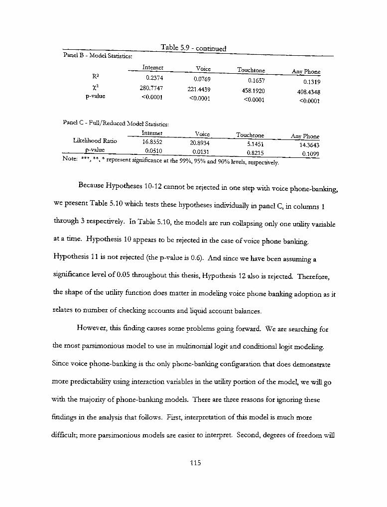
Panel B - Model Statistics:
Internet
R^ 0.2374
y} W^niM p-value <0.0001
Panel C - Full/Reduced Model Statistics:
Internet Likelihood Ratio 16.8552
p-value 0.0510
Voice
0.0769
221.4439
<0.0001
Voice
20.8934
0.0131
Touchtone
0.1657
458.1920
<0.0001
Touchtone
5,1451
0.8215
0,1319
408,4348
<0,0001
Any Phone
14,3643 0.1099
Note: ***, **, * represent significance at die 99%, 95% and 90% levels, respectively.
Because Hypotiieses 10-12 cannot be rejected ki one step witii voke phone-bankkig,
we present Table 5.10 which tests tiiese hypotiieses kidividuaUy ki panel C, ki columns 1
tiirough 3 respectively. In Table 5.10, tiie models are run coUapskig only one utiHty variable
at a time. Hypotiiesis 10 appears to be rejected ki die case of voice phone bankkig.
Hypothesis 11 is not rejected (die p-value is 0.6). And skice we have been assumkig a
significance level of 0.05 duroughout tiks tiiesis, Hypodiesis 12 also is rejected. Therefore,
the shape of the utiHty function does matter in modeHng voice phone bankkig adoption as it
relates to number of checking accounts and hquid account balances.
However, this finding causes some problems going forward. We are searching for
the most parsimonious model to use in multinomial logit and conditional logit modeling.
Since voice phone-banking is the only phone-banking configuration that does demonstrate
more predictabihty using kiteraction variables in the utiHty portion of the model, we wiU go
with the majority of phone-banking models. There are three reasons for ignoring these
findings in the analysis that foUows. Fkst, interpretation of this model is much more
difficult; more parsimonious models are easier to interpret. Second, degrees of freedom -wiU
115
become more knportant in multinomial models; even if the model can be estimated with so
many variables it would not be as powerful. And thkd, the other types of phone-banking
passed this hurdle; we do not want to have to run a different model for each kkid of phone-
banking, just the most parsimonious model for phone-banking in general.
To test whether risk can be represented by one variable, we again use a
fuU/restricted model framework. This tests Hypothesis 13. The results of the reduced
model are found in Table 5.10. As before, panel A contains coefficient estimates and Wald
test statistics. Panel B contains statistics of overaU model fit. Panel C contains the test of
Hypothesis 13 for the four different models. Note that the risk variable can be coUapsed
into one variable only for the Internet banking model. The reason for the difference in
predictive power of individual risk aversion measures may be best seen in the differences
shown ki Table 5.7 of the descriptive statistics section, panel B. The predictive power for 2
and 4 seemed to be higher than that of 1 and 3 for phone bankkig. The discriminating
power of the risk aversion variables were monotonic in the Internet data of that same panel.
The risk variables do have the right sign and are significant for remote channels uskig tiks
model.
Most of the other variables work as hypothesized, aldiough some of die education
variables are not quite as clear as tiiey were ki die previous model. To test for functional
correctness, we test two additional models testing functional form.
116
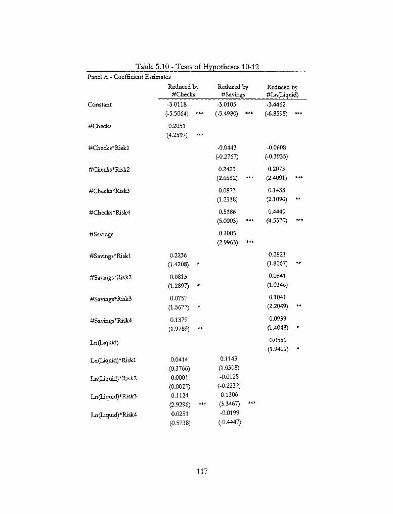
Table 5.10 - Tests of Hypotiieses 10-12 Panel A - Coefficient Estimates
Constant
#Checks
#Checks*Riskl
#Checks*Risk2
#Checks*Risk3
#Checks*Risk4
#Savings
#Savings*Riskl
#Savings*Risk2
#Savings*Risk3
#Savings*Risk4
Ln(Liquid)
Ln(Liquid)*Riskl
Ln(Liquid)*Risk2
Ln(Uquid)*Risk3
Ln(Liquid)*Risk4
Reduced by #Checks
-3.0118
(-5.5064) ***
0.2051
(4.2597) ***
0.2236
(1,4208) *
0,0813
(1,2897) *
0.0757
(1,5677) *
0,1379
(1,9789) **
0,0414
(0.3766)
0,0001
(0,0023)
0.1124
(2.9296) ***
0.0251
(0,5738)
Reduced by #Savings
-3,0105
(-5,4980) ***
-0,0443
(-0,2767)
0,2423
(2,6662) ***
0,0873
(1.2318)
0,5186
(5,0003) **»
0.1005
(2.9963) ***
0.1143
(1.0308)
-0.0128
(-0,2232)
0,1306
(3.3467) ***
-0,0199
(-0,4447)
Reduced by #Ln(Liquid)
-3,4462
(-6,8598) *•*
-0,0608
(-0,3935)
0,2073
(2.4091) ***
0,1433
(2,1090) **
0,4440
(4.5370) ***
0.2821
(1,8067) **
0,0641
(1,0346)
0,1041
(2,2049) **
0,0939
(1,4048) *
0,0551
(1,9411) *
117
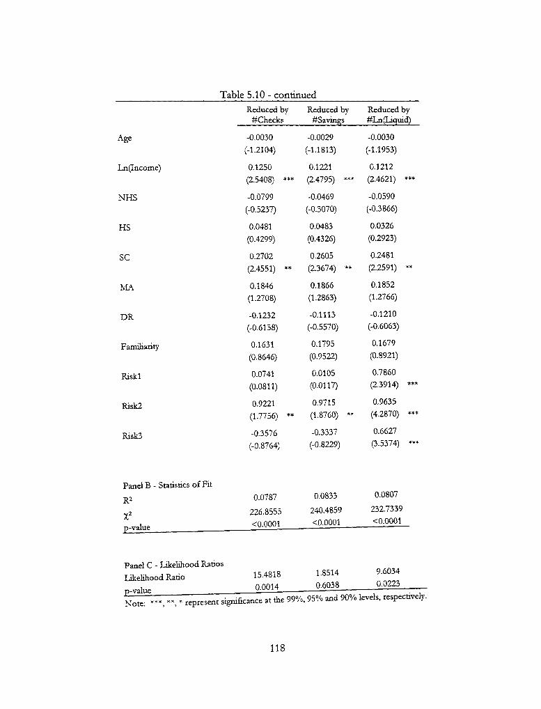
Table 5,10 - continued
Age
Ln (Income)
NHS
HS
SC
MA
DR
Familiarity
Riskl
Risk2
Risk3
Panel B - Statistics of Fit
R2
p-value
Reduced by #Checks
-0,0030
(-1,2104)
0,1250
(2,5408) ***
-0.0799
(-0,5237)
0,0481
(0,4299)
0,2702
(2,4551) **
0.1846
(1.2708)
-0,1232
(-0,6158)
0,1631
(0,8646)
0,0741
(0.0811)
0.9221
(1.7756) **
-0.3576
(-0.8764)
0.0787
226,8555
<0.0001
Reduced by #Savings
-0,0029
(-1,1813)
0.1221
(2.4795) ***
-0.0469
(-0,3070)
0,0483
(0,4326)
0,2605
(2,3674) **
0.1866
(1,2863)
-0,1113
(-0,5570)
0,1795
(0,9522)
0,0105
(0.0117)
0.9715
(1.8760) **
-0.3337
(-0.8229)
0.0833
240,4859
<0.0001
Reduced by #Ln (Liquid)
-0,0030
(-1,1953)
0,1212
(2,4621) ***
-0.0590
(-0,3866)
0,0326
(0,2923)
0,2481
(2,2591) **
0,1852
(1,2766)
-0,1210
(-0,6063)
0,1679
(0,8921)
0,7860
(2,3914) ***
0,9635
(4,2870) ***
0.6627
(3,5374) ***
0,0807
232.7339
<0.0001
Panel C - Jikeliliood Ratios
Likelihood Ratio
p-value ^ — Note: ***. **, * represent significance at die 99%, 95% and 90% levels, respectively.
15.4818
0.0014
1.8514
0.6038
9.6034
0.0223
118
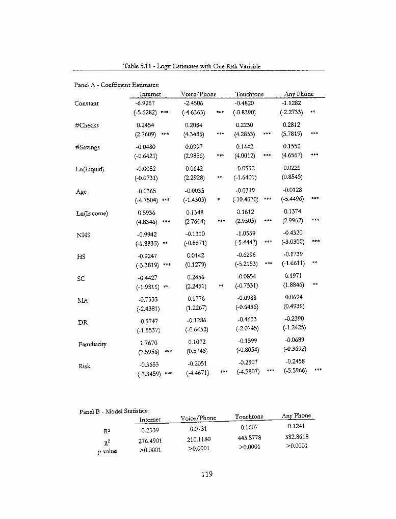
Table 5.11 - Logit Estimates with One Risk Variable
Panel A - Coefficient Estimates:
Constant
#Checks
#Savings
Ln (Liquid)
Age
Ln (Income)
NHS
HS
SC
MA
DR
Familiarity
Risk
Internet
-6.9267
(-5.6282) ***
0,2454
(2,7609) ***
-0,0480
(-0,6421)
-0.0052
(-0,0731)
-0,0365
(-4,7504) ***
0.5936
(4.8346) ***
-0.9942
(-1,8835) **
-0,9247
(-3,3819) ***
-0,4427
(-1.9811) **
-0,7333
(-2,4381)
-0.5747
(-1,5537)
1,7670
(7,5956) ***
-0,3653
(-3.3459) ***
Voice/Phone
-2,4506
(-4,6363) ***
0,2084
(4,3486)
0.0997
(2.9856) ***
0.0642
(2.2928)
-0.0035
(-1,4303) *
0,1348
(2,7604) ***
-0,1310
(-0,8671)
0,0142
(0,1279)
0.2456
(2,2451)
0.1776
(1,2267)
-0,1286
(-0.6452)
0,1072
(0,5746)
-0,2051
(-4.4671) ***
Touchtone
-0,4820
(-0,8390)
0,2230
(4.2853) ***
0,1442
(4,0012) ***
-0,0532
(-1,6401)
-0,0319
(-10.4070) ***
0.1612
(2.9505) ***
-1.0559
(-5.4447) ***
-0.6296
(-5.2153) ***
-0.0854
(-0,7531)
-0,0988
(-0,6436)
-0,4633
(-2.0745)
-0,1599
(-0,8054)
-0,2307
(-4,5807) **•
Any Phone
-1,1282
(-2,2733) **
0,2812
(5,7819) ***
0,1552
(4,6567) ***
0,0229
(0,8545)
-0,0128
(-5.4496) ***
0,1374
(2,9962) ***
-0,4320
(-3,0300) ***
-0.1739
(-1.6611) **
0.1971
(1.8846) **
0,0694
(0,4939)
-0,2390
(-1,2425)
-0,0689
(-0,3692)
-0,2458
(-5,5966) ***
Panel B - Model Statistics: Internet
R2
p-value
0,2339
276,4901
>0,0001
Voice/Phone
0,0731
210,1180
>0,0001
Touchtone
0.1607
443,5778
>0.0001
^\ny Phone
0,1241
382,8618
>0,0001
119
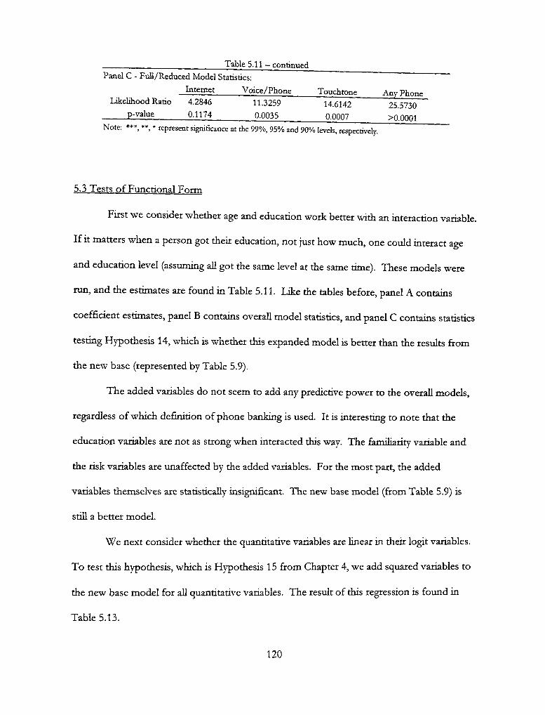
Table 5,11 - continued Panel C - Full/Reduced Model Statistics:
Internet Voice/Phone Touchtone Any Phone Likelihood Ratio 4,2846 11,3259 14,6142 25,5730
P-value 0,1174 0,0035 0,0007 >o.oooi Note: ***, **, " represent significance at the 99%, 95% and 90% levels, respectively.
5.3 Tests of Functional Form
Fkst we consider whedier age and education work better witii an kiteraction variable.
If k matters when a person got tiiek education, not just how much, one could kiteract age
and education level (assumkig aU got the same level at tiie same time). These models were
run, and die estimates are found in Table 5.11. l ike die tables before, panel A contams
coefficient estknates, panel B contakis overaU model statistics, and panel C contains statistics
testkig Hypothesis 14, which is whether this expanded model is better than the results from
the new base (represented by Table 5.9).
The added variables do not seem to add any predictive power to the overaU models,
regardless of which definition of phone banking is used. It is interesting to note that the
education variables are not as strong when interacted this way. The famiHarity variable and
the risk variables are unaffected by the added variables. For the most part, the added
variables themselves are statisticaUy insignificant. The new base model (from Table 5.9) is
StiU a better model.
We next consider whether the quantitative variables are linear in thek logit variables.
To test this hypothesis, which is Hypothesis 15 from Chapter 4, we add squared variables to
the new base model for aU quantitative variables. The result of this regression is foimd in
Table 5.13.
120
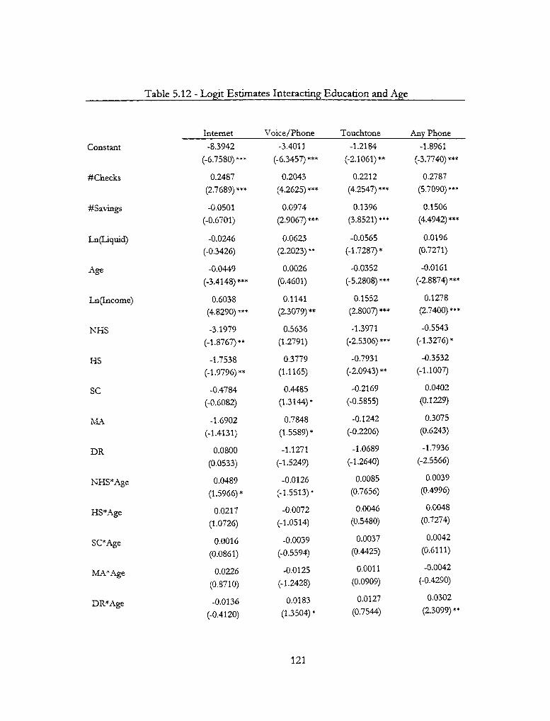
Table 5.12 - Logit Estknates Interacting Education and Age
Constant
#Checks
#Savings
Ln (Liquid)
Age
Ln (Income)
NHS
HS
SC
MA
DR
NHS*Age
HS*-'»i.ge
SC*Age
MA*Age
DR*Age
Internet
-8.3942
(-6.7580) ***
0.2487
(2.7689)***
-0.0501
(-0.6701)
-0.0246
(-0.3426)
-0.0449
(-3.4148)***
0.6038
(4.8290)***
-3.1979
(-1.8767)**
-1,7538
(-1,9796)**
-0,4784
(-0,6082)
-1.6902
(-1,4131)
0,0800
(0.0533)
0.0489
(1.5966)*
0.0217
(1,0726)
0.0016
(0,0861)
0,0226
(0,8710)
-0,0136
(-0.4120)
Voice/Phone
-3,4011
(-6.3457) ***
0,2043
(4,2625)***
0,0974
(2,9067) ***
0,0623
(2,2023)**
0,0026
(0.4601)
0,1141
(2,3079)**
0,5636
(1,2791)
0.3779
(1.1165)
0,4485
(1,3144)*
0,7848
(1.5589)*
-1.1271
(-1,5249)
-0.0126
(-1.5513)*
-0.0072
(-1.0514)
-0,0039
(-0,5594)
-0,0125
(-1,2428)
0.0183
(1.3504)*
Touchtone
-1.2184
(-2,1061)**
0,2212
(4,2547) ***
0,1396
(3,8521)***
-0,0565
(-1,7287)*
-0,0352
(-5,2808)***
0,1552
(2,8007) ***
-1,3971
(-2,5306)***
-0,7931
(-2,0943)**
-0.2169
(-0,5855)
-0.1242
(-0.2206)
-1.0689
(-1.2640)
0,0085
(0,7656)
0.0046
(0,5480)
0.0037
(0,4425)
0,0011
(0,0909)
0,0127
(0,7544)
Any Phone
-1,8961
(-3,7740)***
0.2787
(5,7090) ***
0,1506
(4,4942)***
0,0196
(0,7271)
-0,0161
(-2,8874)***
0,1278
(2,7400)***
-0.5543
(-1.3276)*
-0.3532
(-1.1007)
0,0402
(0,1229)
0.3075
(0,6243)
-1,7936
(-2,5566)
0,0039
(0,4996)
0,0048
(0,7274)
0,0042
(0,6111)
-0,0042
(-0,4290)
0,0302
(2,3099)**
121
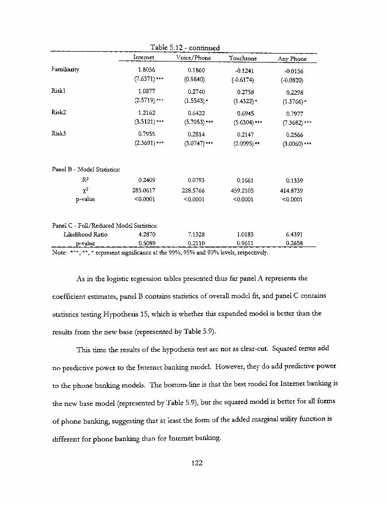
Table 5.12 - continued
Familiarity
Riskl
Risk2
Risk3
Panel B - Model Statistics:
R2
t p-value
Internet
1.8056
(7.6371)***
1.0877
(2.5719)***
1.2162
(3.5121)***
0.7955
(2.3691) ***
0.2409
285.0617
<0.0001
Voice/Phone
0,1860
(0,9840)
0,2740
(1,5543)*
0,6422
(5,7053)***
0,2814
(3,0747) ***
0,0793
228,5766
<0,0001
Touchtone
-0,1241
(-0,6174)
0.2758
(1.4322)*
0.6945
(5,6304)***
0,2147
(2,0095) **
0,1661
459,2105
<0,0001
Any Phone
-0,0156
(-0,0820)
0,2298
(1,3766)*
0,7977
(7,3682)***
0,2566
(3,0060) ***
0,1339
414,8739
<0,0001
Panel C - Full/Reduced Model Statistics:
Likelihood Ratio 4,2870
p-value 0,5089
7,1328
0,2110
1,0185
0,9611
6,4391
0.2658
Note: ***, **, * represent sig;nificance at the 99%, 95% and 90% levels, respectively.
As in the logistic regression tables presented thus far panel A represents the
coefficient estknates, panel B contakis statistics of overaU model fit, and panel C contains
statistics testing Hj-pothesis 15, which is whether this expanded model is better than the
resiUts from the new base (represented by Table 5.9).
This time the results of the hypothesis test are not as clear-cut. Squared terms add
no predictive power to the Internet bankkig model. However, tiiey do add predictive power
to the phone bankkig models. The bottom-hne is tiiat tiie best model for Internet bankkig is
die new base model (represented by Table 5.9), but die squared model is better for aU forms
of phone bankkig, suggesting that at least tiie form of tiie added margkial utihty function is
different for phone banking than for Internet banking.
122
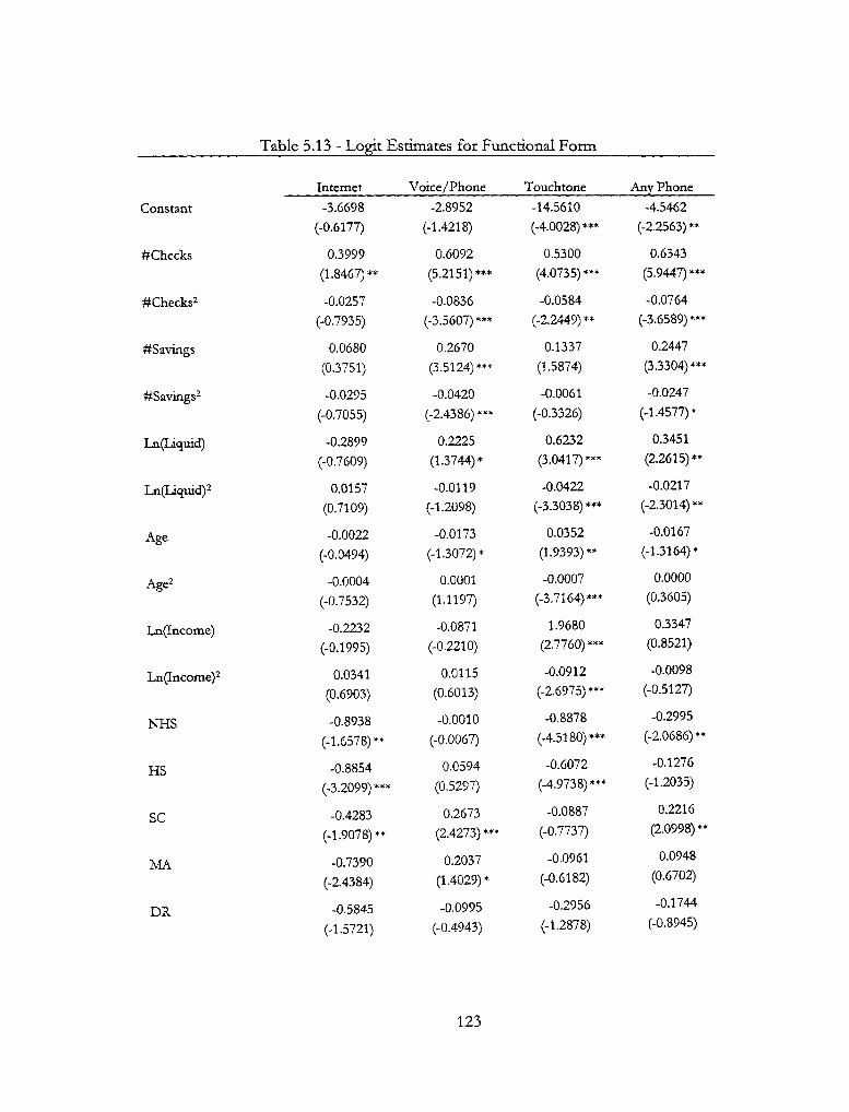
Table 5.13 - Logit Estimates for Functional Form
Constant
#Checks
#Checks2
#Savings
#Savings^
Ln(Liquid)
Ln(Liquid)2
Age
Age^
Ln(Income)
Ln(Income)^
NHS
HS
SC
MA
DR
Internet
-3.6698
(-0.6177)
0.3999
(1.8467)**
-0.0257
(-0,7935)
0,0680
(0,3751)
-0,0295
(-0,7055)
-0,2899
(-0,7609)
0,0157
(0,7109)
-0,0022
(-0,0494)
-0,0004
(-0,7532)
-0.2232
(-0.1995)
0.0341
(0.6903)
-0.8938
(-1.6578)**
-0.8854
(-3.2099)***
-0.4283
(-1.9078)**
-0.7390
(-2.4384)
-0.5845
(-1.5721)
Voice/Phone
-2.8952
(-1.4218)
0.6092
(5.2151)***
-0.0836
(-3.5607)***
0,2670
(3,5124)***
-0,0420
(-2,4386)***
0,2225
(1,3744)*
-0,0119
(-1,2098)
-0,0173
(-1,3072)*
0,0001
(1,1197)
-0,0871
(-0.2210)
0,0115
(0,6013)
-0,0010
(-0,0067)
0.0594
(0.5297)
0,2673
(2,4273)***
0,2037
(1,4029)*
-0,0995
(-0,4943)
Touchtone
-14,5610
(-4,0028) »**
0.5300
(4,0735)***
-0,0584
(-2,2449)**
0,1337
(1,5874)
-0,0061
(-0,3326)
0,6232
(3,0417)***
-0,0422
(-3,3038)***
0,0352
(1,9393)**
-0,0007
(-3,7164)***
1,9680
(2,7760)***
-0.0912
(-2,6975)***
-0,8878
(-4,5180)***
-0,6072
(-4,9738)***
-0,0887
(-0,7737)
-0.0961
(-0,6182)
-0,2956
(-1,2878)
Any Phone
-4,5462
(-2,2563)**
0,6343
(5.9447) ***
-0,0764
(-3,6589)***
0,2447
(3.3304)***
-0.0247
(-1.4577)*
0.3451
(2.2615)**
-0.0217
(-2.3014)**
-0.0167
(-1.3164)*
0,0000
(0,3605)
0,3347
(0,8521)
-0,0098
(-0,5127)
-0,2995
(-2,0686)**
-0,1276
(-1.2035)
0,2216
(2,0998)**
0,0948
(0.6702)
-0,1744
(-0,8945)
123
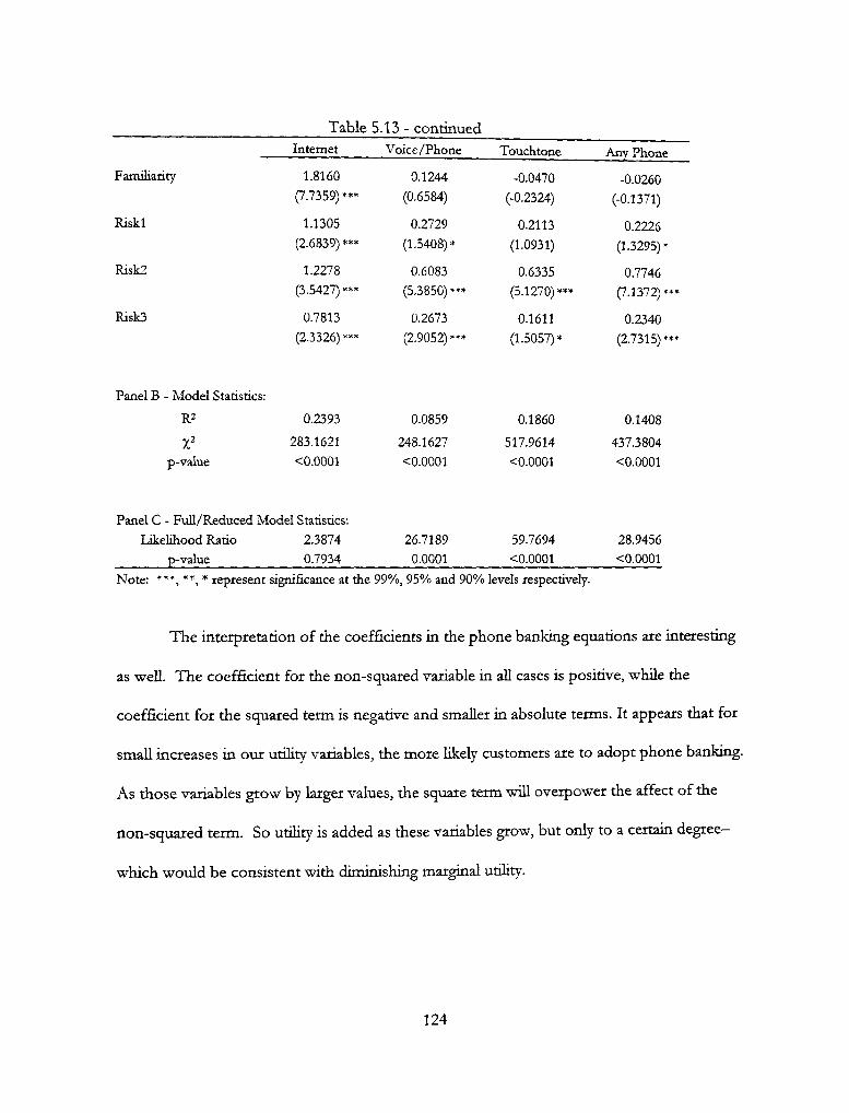
Table 5,13 - continued
Familiarity
Riskl
Risk2
Risk3
Panel B • - Model Statistics:
R2
X p-value
Internet
1,8160
(7,7359) ***
1,1305
(2,6839) ***
1,2278
(3,5427) *»*
0,7813
(2,3326)***
0,2393
283,1621
<0.0001
Voice/Phone
0,1244
(0,6584)
0,2729
(1,5408)*
0,6083
(5,3850)***
0,2673
(2,9052)***
0,0859
248,1627
<0,0001
Touchtone
-0,0470
(-0,2324)
0,2113
(1,0931)
0,6335
(5,1270)***
0,1611
(1,5057)*
0,1860
517,9614
<0,0001
Any Phone
-0,0260
(-0,1371)
0,2226
(1,3295)*
0,7746
C7,1372) ***
0,2340
(2,7315)***
0,1408
437,3804
<0,0001
Panel C - Full/Reduced Model Statistics:
Likelihood Ratio 2,3874 26.7189 59,7694 28,9456
p-value 0,7934 0,0001 <0,0001 <0,0001
Note: ***, **, * represent significance at the 99%, 95% and 90% levels respectively.
The interpretation of the coefficients in the phone banking equations are interesting
as weU. The coefficient for the non-squared variable in aU cases is positive, whUe the
coefficient for the squared term is negative and smaUer in absolute terms. It appears that for
smaU increases in our utiHty variables, the more hkely customers are to adopt phone banking.
As those variables grow by larger values, the square term wiU overpower the affect of the
non-squared term. So utUity is added as these variables grow, but oiUy to a certain degree-
which would be consistent with diminishkig marginal utihty.
124
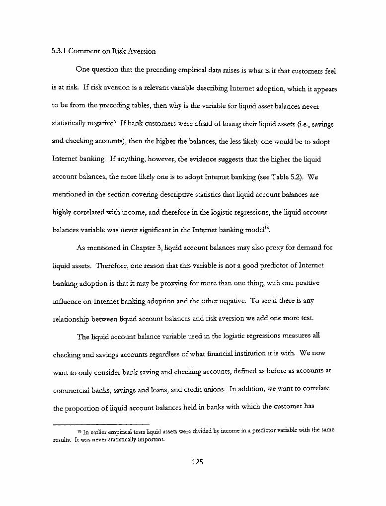
5.3.1 Comment on Risk Aversion
One question that the preceding empkical data raises is what is it that customers feel
is at risk. If risk aversion is a relevant variable describkig Internet adoption, which it appears
to be from the preceding tables, then why is the variable for Hquid asset balances never
StatisticaUy negative? If bank customers were afraid of losing thek Hquid assets (i.e., savings
and checking accounts), then the higher the balances, the less hkely one would be to adopt
Internet banking. If anything, however, the evidence suggests that the higher the Hquid
account balances, the more hkely one is to adopt Internet banking (see Table 5.2). We
mentioned in the section covering descriptive statistics that Hquid account balances are
highly correlated with income, and therefore in the logistic regressions, the Hquid account
balances variable was never significant in the Internet banking model'*.
As mentioned in Chapter 3, hquid account balances may also proxy for demand for
hquid assets. Therefore, one reason that this variable is not a good predictor of Internet
banking adoption is that it may be proxying for more than one thing, with one positive
influence on Internet banking adoption and the other negative. To see if there is any
relationship between hquid account balances and risk aversion we add one more test.
The Hquid account balance variable used ki the logistic regressions measures aU
checking and savings accounts regardless of what financial institution k is with. We now
want to only consider bank saving and checkkig accovmts, defined as before as accounts at
commercial banks, savkigs and loans, and credit unions. In addition, we want to correlate
the proportion of Hquid account balances held ki banks witii which tiie customer has
18 In earlier empirical tests liquid assets were divided by income in a predictor variable widi die same
results. It was never statistically important.
125
Internet access witii the risk level. If customers perceive tiiat tiie Hquid assets held ki banks
witii Internet access are more risky, then diere should be a negative correlation between die
proportion of hquid assets ki banks witii Internet access and die customers risk aversion
number:
Table 5.14 contakis tiie correlation coefficient estimates for risk aversion vis-a-vis
proportion of Hquid assets held in banks witii Internet access. As ki the text thus far, we wUl
treat risk aversion as a quantitative variable and as an ordinal measure. The Pearson
correlation treats risk aversion as a quantitative variable. The Spearman's Rho and KenaU's
Tau are non-parametric correlations used with ordkial data. But even with these measures,
there is no evidence of relationship between hquid account balances and risk aversion. Even
though risk aversion is important to the Intemet adoption decision, there is no evidence that
risk aversion has anything to do with fear of losing money through the customer's bank
account.
Table 5.14 — Correlation Between Proportion of Liquid Account Balances in an Intemet Bank and Risk Aversion
Coefficient Estimate P-Value
Pearson's Correlation -0.0490 0.2692
KendaU'sTau -0.0581 0.1890
Spearman's Rho -0.0684 0.1885
126
5.4 Multinomial Model
As mentioned in Chapter 3, the variables used in this chapter should affect the
probabihty that bank customers faU into four different categories shown on Table 4.1. In
this section, we present the results from two multinomial logistic regressions. The first
presents what we have caUed the new base model, represented in bivariate form in Table 5.9.
This form was the best model for the Internet banking appHcation. The second multinomial
logistic regression model presented is the base model with squared quantitative terms. This
second model was the best bivariate form for phone bankkig. These models wiU then be
fvirtiier used to estimate the marginal propensity to adopt in the next section.
Table 5.15 presents the overaU statistics of fit for the base multinomial regression
model. The columns represent different definitions of phone-banking (in other words, the
model was run three times). Panel A uses a fuU/reduced model methodology to test the
sigikficance of individual variables in the multinomial model. The statistic presented for
each variable is the chi-squared hkehhood ratio. The figure in parenthesis is the p-value.
With the exception of Ln(Liquid), which measures the amount of hquid asset balances held
by the customer, aU variables are statisticaUy significant with at least one definition of phone-
banking.
Panel B presents overaU statistics of fit for the new base model with phone-banking
defined as described in the column headings. The chi-squared statistic is a test of
Hypothesis 16 from Chapter 4, Note that in each case the hypothesis is rejected. In other
words, these variables appear to have some predictive power in determining the remote
banking solution chosen by bank customers.
127
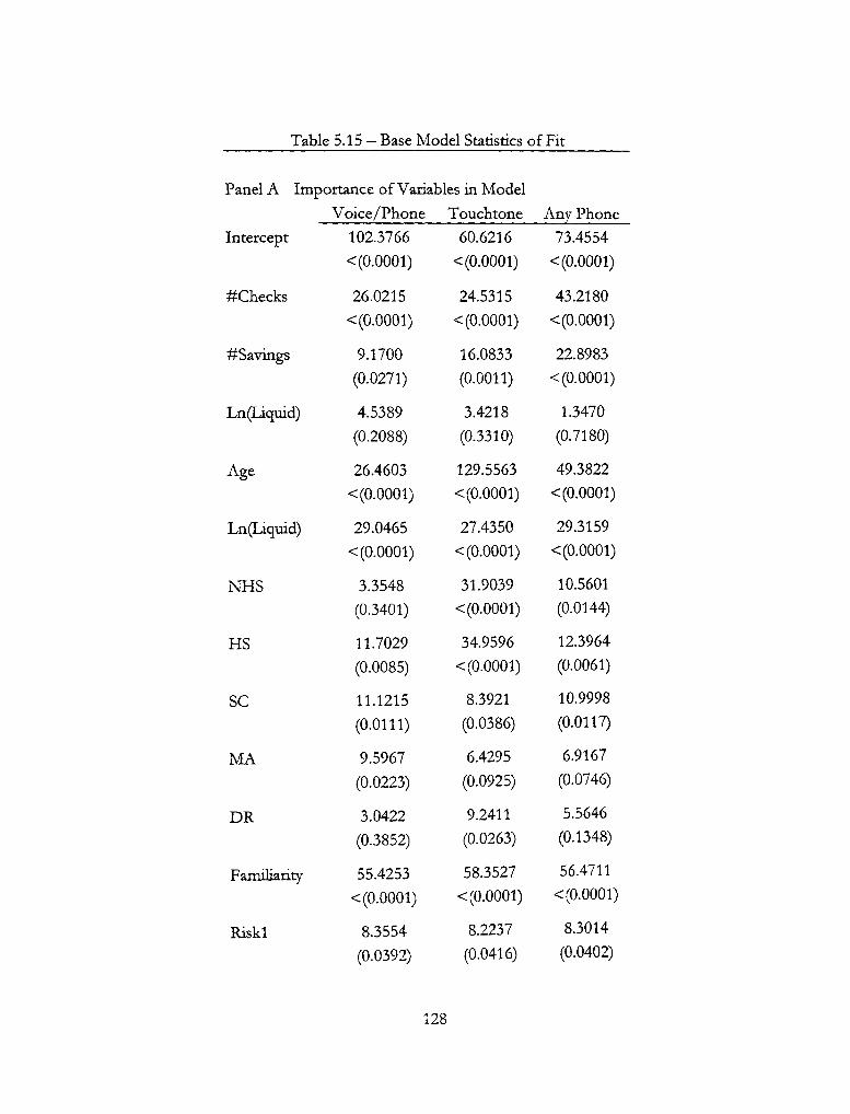
Table 5.15 - Base Model Statistics of Fit
Panel A Importance of Variables in Model
Intercept
#Checks
#Savings
Ln(Liquid)
Age
Ln (Liquid)
NHS
HS
SC
MA
DR
Familiarity
Riskl
Voice/Phone
102.3766
<(0.0001)
26.0215
< (0.0001)
9.1700
(0.0271)
4.5389
(0.2088)
26.4603
<(0.0001)
29.0465
< (0.0001)
3.3548
(0.3401)
11.7029
(0.0085)
11.1215
(0.0111)
9.5967
(0.0223)
3.0422
(0.3852)
55.4253
<(0.0001)
8.3554
(0,0392)
Touchtone
60.6216
< (0.0001)
24.5315
< (0.0001)
16.0833
(0.0011)
3.4218
(0.3310)
129.5563
<(0.0001)
27.4350
< (0.0001)
31.9039
<(0.0001)
34,9596
< (0.0001)
8.3921
(0.0386)
6.4295
(0.0925)
9.2411
(0.0263)
58.3527
<(0.0001)
8.2237
(0.0416)
Any Phone
73.4554
< (0.0001)
43.2180
<(0.0001)
22.8983
< (0.0001)
1.3470
(0.7180)
49.3822
<(0.0001)
29.3159
< (0.0001)
10.5601
(0.0144)
12.3964
(0.0061)
10.9998
(0.0117)
6.9167
(0.0746)
5.5646
(0.1348)
56.4711
<(0.0001)
8.3014
(0.0402)
128
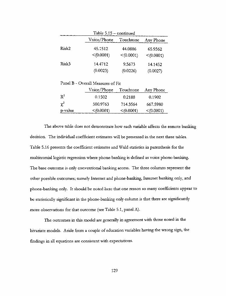
Table 5.15 - continued
Voice/Phone Touchtone Any Phone
Risk2 45.1512 44.0886 65.9362
<(0.0001) <(0.0001) <(0.0001)
Risk3 14.4712 9.5673 14.1452
(0.0023) (0.0226) (0.0027)
Panel B - OveraU Measures of Fit
Voice/Phone Touchtone Any Phone
R' 0.1502 0.2188 0.1902
t 500.9763 714.3564 667.5980
p-value <(0.0001) <(0.0001) <(0.0001)
The above table does not demonstrate how each variable affects the remote banking
decision. The individual coefficient estimates wiU be presented in the next three tables.
Table 5.16 presents the coefficient estimates and Wald statistics in parenthesis for the
multinomial logistic regression where phone-banking is defined as voice phone-banking.
The base outcome is only conventional bankkig access. The three columns represent the
other possible outcomes; namely Intemet and phone-banking, Intemet banking only, and
phone-banking oiUy. It should be noted here that one reason so many coefficients appear to
be StatisticaUy significant in the phone-bankkig only column is that there are significantiy
more observations for that outcome (see Table 5.1, panel A).
The outcomes in this model are generaUy in agreement with those noted in the
bivariate models. Aside from a couple of education variables having the wrong sign, the
findings in aU equations are consistent with expectations.
129
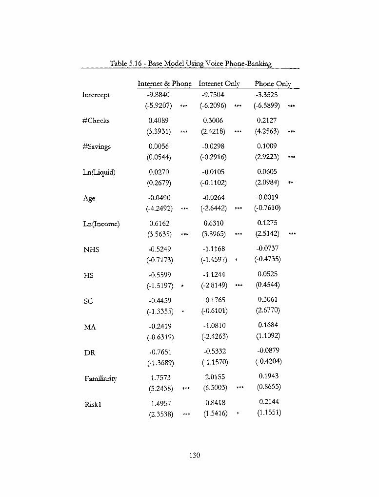
Table 5.16 - Base Model Using Voice Phone-Banking
Intercept
#Checks
#Savings
Ln (Liquid)
Age
Ln(Income)
NHS
HS
SC
MA
DR
FamiHarity
Riskl
Internet & Phone
-9.8840
(-5.9207)
0.4089
(3.3931)
0.0056
(0.0544)
0.0270
(0.2679)
-0.0490
(-4.2492)
0.6162
(3.5635)
-0.5249
(-0.7173)
-0.5599
(-1.5197)
-0.4459
(-1.3355)
-0.2419
(-0.6319)
-0.7651
(-1.3689)
1.7573
(5.2438)
1.4957
(2.3538)
*Y'^
***
***
***
*
*
^-.*.*
***
Intemet Only
-9.7504
(-6.2096)
0.3006
(2.4218)
-0.0298
(-0.2916)
-0.0105
(-0.1102)
-0.0264
(-2.6442)
0.6310
(3.8965)
-1.1168
(-1.4597)
-1.1244
(-2.8149)
-0.1765
(-0.6101)
-1.0810
(-2.4263)
-0.5332
(-1.1570)
2.0155
(6.5003)
0.8418
(1.5416)
***
***
***
***
*
***
***
*
Phone Only
-3.3525
(-6.5899) ***
0.2127
(4.2563) ***
0.1009
(2.9223) ***
0.0605
(2.0984) **
-0.0019
(-0.7610)
0.1275
(2.5142) *»*
-0.0737
(-0.4735)
0.0525
(0.4544)
0.3061
(2.6770)
0.1684
(1.1092)
-0.0879
(-0.4204)
0.1943
(0.8655)
0.2144
(1.1551)
130
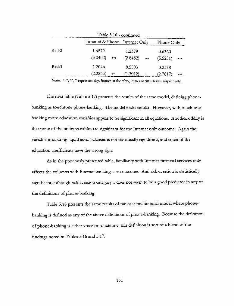
Table 5.16 - continued
Intemet & Phone Intemet Only Phone Only
RiskZ 1.6879 1.2379 0.6360
(3.0402) *** (2.8482) *** (5.5251) ***
Risk3 1.2044 0.5503 0.2578
(2.2255) ** (1.3012) * (2.7817) ***
Note: ***, **, * represent significance at the 99%), 95% and 90% levels respectively.
The next table (Table 5.17) presents the results of the same model, defining phone-
banking as touchtone phone-banking. The model looks similar. However, with touchtone
banking more education variables appear to be significant in aU equations. Another oddity is
that none of the utiHty variables are significant for the Intemet only outcome. Again the
variable measuring Hquid asset balances is not statisticaUy significant, and some of the
education coefficients have the wrong sign.
As in the previously presented table, famiharitjr with Intemet financial services only
affects the columns with Intemet banking as an outcome. And risk aversion is statisticaUy
significant, although risk aversion category 1 does not seem to be a good predictor in any of
the definitions of phone-banking.
Table 5.18 presents the same results of tiie base multkiomial model where phone-
banking is defined as any of the above definitions of phone-bankkig. Because the defiiktion
of phone-bankkig is either voice or touchtone, this definition is sort of a blend of die
findings noted in Tables 5.16 and 5.17.
131
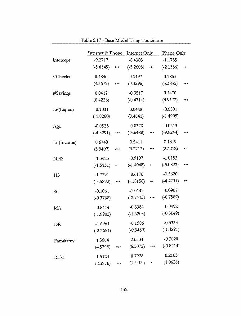
Table 5.17 - Base Model Using Touchtone
Intercept
#Checks
#Savings
Ln (Liquid)
Age
Ln(Income)
NHS
HS
SC
MA
DR
FamUiarity
Riskl
Intemet & Phone
-9.2717
(-5.6549)
0.4840
(4.3672)
0.0417
(0.4228)
-0.1031
(-1.0260)
-0.0525
(-4.5291)
0.6740
(3.9407)
-1.3923
(-1.5131)
-1.7791
(-3.5892)
-0.1061
(-0.3768)
-0.8414
(-1.9905)
-1.6961
(-2.3651)
1.5064
(4.5798)
1.5124
(2.3876)
***
¥ * *
***
***
*
***
***
+*=t
Intemet Only
-8.4303
(-5.2603)
0.0497
(0.3296)
-0.0517
(-0.4714)
0.0448
(0.4641)
-0.0370
(-3.6488)
0.5411
(3.2713)
-0.9197
(-1.4048)
-0.6176
(-1.8156)
-1.0147
(-2.7413)
-0.6384
(-1.6203)
-0.1506
(-0.3489)
2.0334
(6.5072)
0.7928
(1.4400)
***
***
***
*
**
***
***
*
Phone Only
-1.1755
(-2.1336) **
0.1865
(3.3835) ***
0.1470
(3.9172) ***
-0.0501
(-1.4905)
-0.0313
(-9.9244) ***
0.1319
(2.3212) **
-1.0152
(-5.0822) ***
-0.5620
(.4.4731) ***
-0.0907
(-0.7589)
-0.0492
(-0.3049)
-0.3333
(-1.4291)
-0.2020
(-0.8214)
0.2165
(1.0628)
132
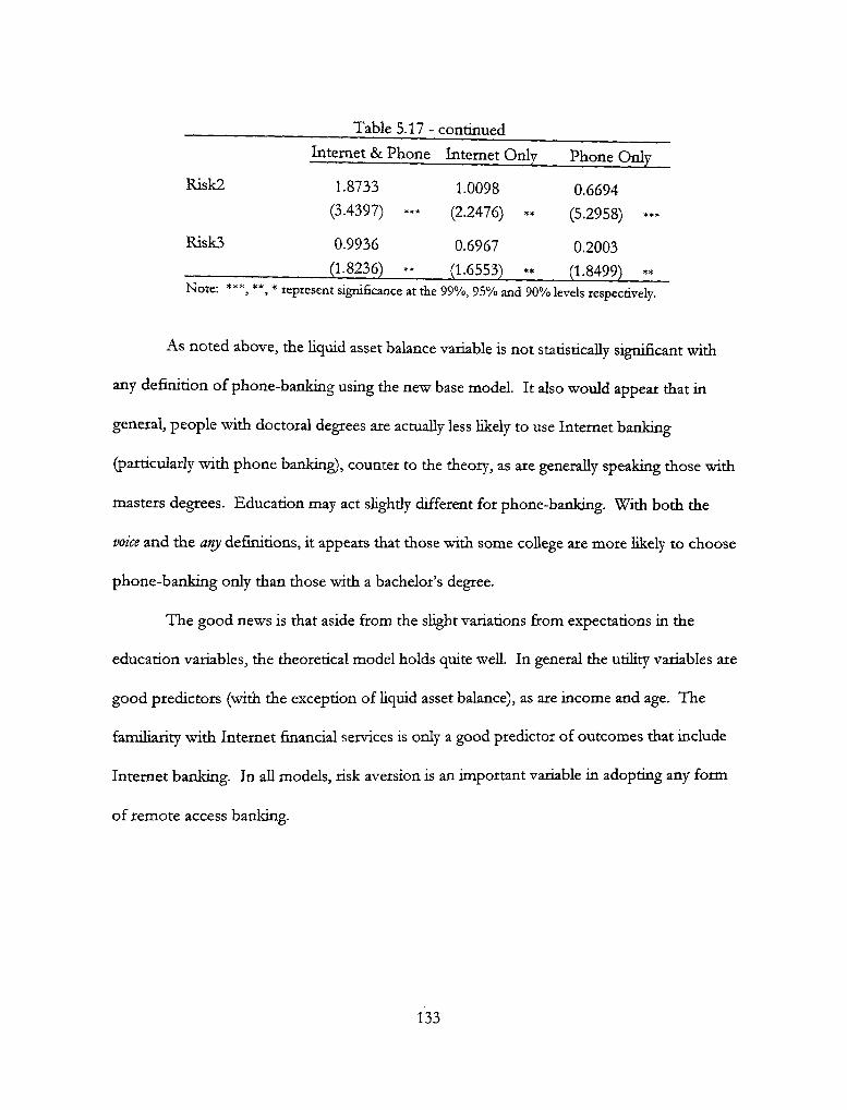
Table 5.17 - continued
Intemet & Phone Intemet Only Phone Only
Risk2 1.8733 1.0098 0.6694
(3.4397) *** (2.2476) *» (5.2958) *-
Risk3 0.9936 0.6967 0.2003
(1.8236) ** (1.6553) ** (1.8499) ** ^ o t e : ***, **, * represent significance at die 99%, 95% and 90% levels respectively.
As noted above, the hquid asset balance variable is not statisticaUy significant viith
any defimtion of phone-banldng using the new base model. It also would appear that in
general, people with doctoral degrees are actuaUy less Hkely to use Intemet bankkig
(particularly with phone banking), counter to the theory, as are generaUy speaking those with
masters degrees. Education may act sHghtiy different for phone-banking. With both the
voice and the any definitions, it appears that those with some coUege are more likely to choose
phone-banking oiUy than those with a bachelor's degree.
The good news is that aside from the slight variations from expectations in the
education variables, the theoretical model holds qviite weU, In general the utiHty variables are
good predictors (with the exception of Hquid asset balance), as are income and age. The
familiarity with Intemet financial services is only a good predictor of outcomes that include
Intemet banking. In aU models, risk aversion is an important variable in adopting any form
of remote access banking.
133
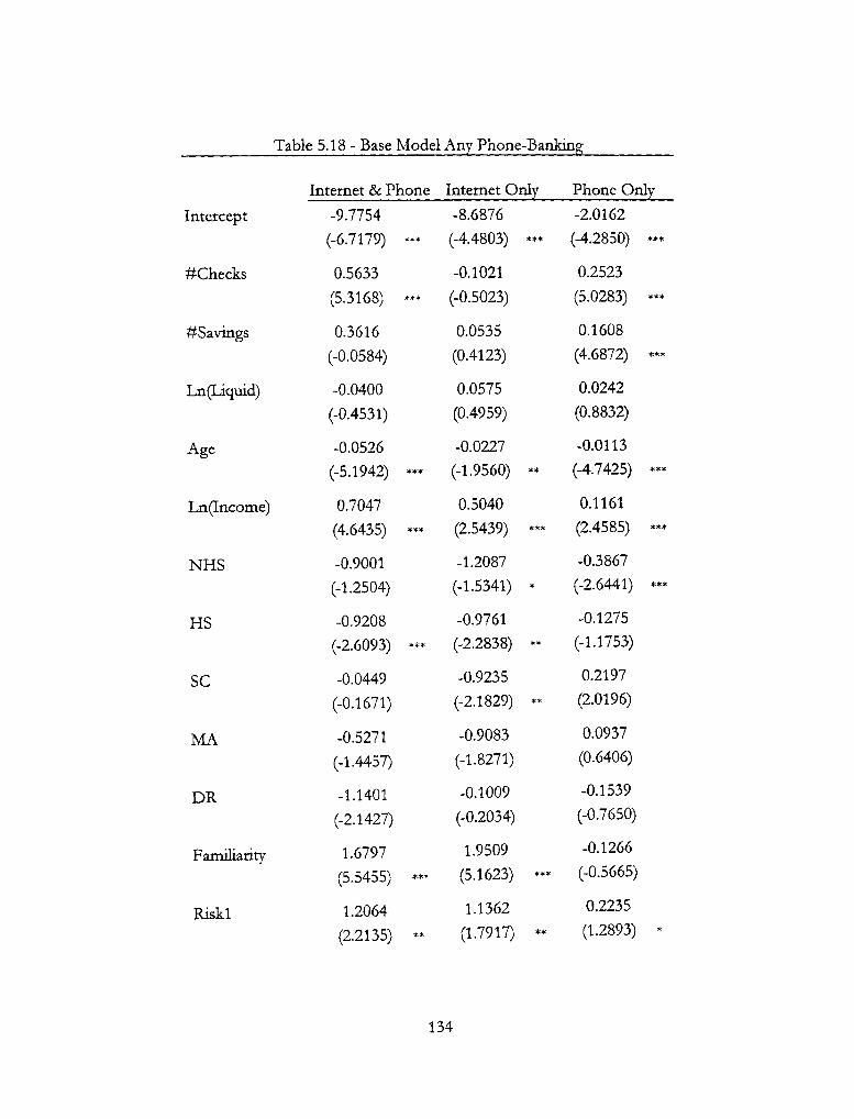
Table 5.18 - Base Model Any Phone-Banking
Intercept
#Checks
#Savings
Ln(Liquid)
Age
Ln(Income)
NHS
HS
SC
MA
DR
FamUiarity
Riskl
Internet & Phone
-9.7754
(-6.7179)
0.5633
(5.3168)
0.3616
(-0.0584)
-0.0400
(-0.4531)
-0.0526
(-5.1942)
0.7047
(4.6435)
-0.9001
(-1.2504)
-0.9208
(-2.6093)
-0.0449
(-0.1671)
-0.5271
(-1.4457)
-1.1401
(-2.1427)
1.6797
(5.5455)
1.2064
(2.2135)
***
***
* ¥ *
***
x * *
***
Intemet Only
-8.6876
(-4.4803) ***
-0.1021
(-0.5023)
0.0535
(0.4123)
0.0575
(0.4959)
-0.0227
(-1.9560) **
0.5040
(2.5439) ***
-1.2087
(-1.5341) *
-0.9761
(-2.2838) **
-0.9235
(-2.1829) **
-0.9083
(-1.8271)
-0.1009
(-0.2034)
1.9509
(5.1623) ***
1.1362
(1.7917) **
Phone Only
-2.0162
(-4.2850) ***
0.2523
(5.0283) ***
0.1608
(4.6872) ***
0.0242
(0.8832)
-0.0113
(-4.7425) ***
0.1161
(2.4585) ***
-0.3867
(-2.6441) ***
-0.1275
(-1.1753)
0.2197
(2.0196)
0.0937
(0.6406)
-0.1539
(-0.7650)
-0.1266
(-0.5665)
0.2235
(1.2893) *
134
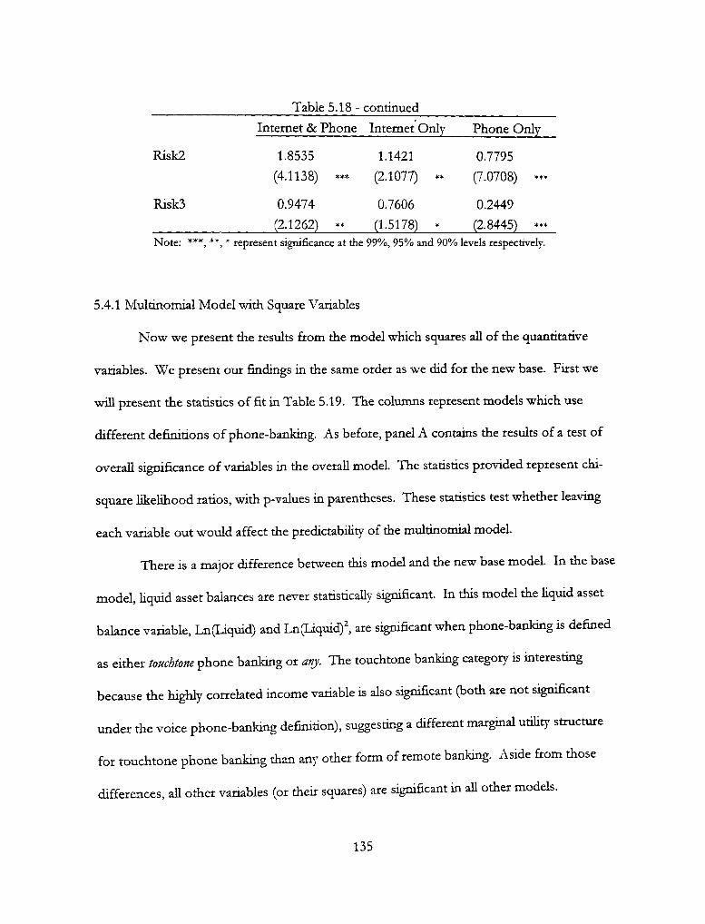
Table 5.18 - continued
Intemet & Phone Intemet OiUy Phone Only
Risk2 1.8535 1.1421 0.7795
(4.1138) *** (2.1077) ** (7.0708) ***
Risk3 0.9474 0.7606 0.2449
(2.1262) ** (1.5178) * (2.8445) *** Note: ***, **, * represent significance at the 99%, 95% and 90% levels respectively.
5.4.1 Multinomial Model with Square Variables
Now we present the resiUts from the model which squares aU of the quantitative
variables. We present our findings in the same order as we did for the new base. Fkst we
wiU present the statistics of fit ki Table 5.19. The columns represent models which use
different defiiiktions of phone-banking. As before, panel A contakis the results of a test of
overaU significance of variables ki the overaU model. The statistics provided represent chi-
square hkehhood ratios, with p-values ki parentiieses. These statistics test whether leavmg
each variable out would affect the predictabihty of the mvUtinomial model.
There is a major difference between tiks model and the new base model. In the base
model, hquid asset balances are never statisticaUy significant. In tiks model die hquid asset
balance variable, Ln(Uquid) and Ln(Liquid)', are significant when phone-bankkig is defined
as eitiier touchtone phone bankkig or any. The touchtone bankkig category is kiteresting
because die highly correlated kicome variable is also significant (botii are not significant
under die voice phone-bankmg definition), suggesting a different margkial utihtj- sdrucmre
for touchtone phone bankkig tiian any otiier form of remote banking. Aside fiom tiiose
differences, aU otiier variables (or tiiek squares) are significant ki aU otiier models.
135
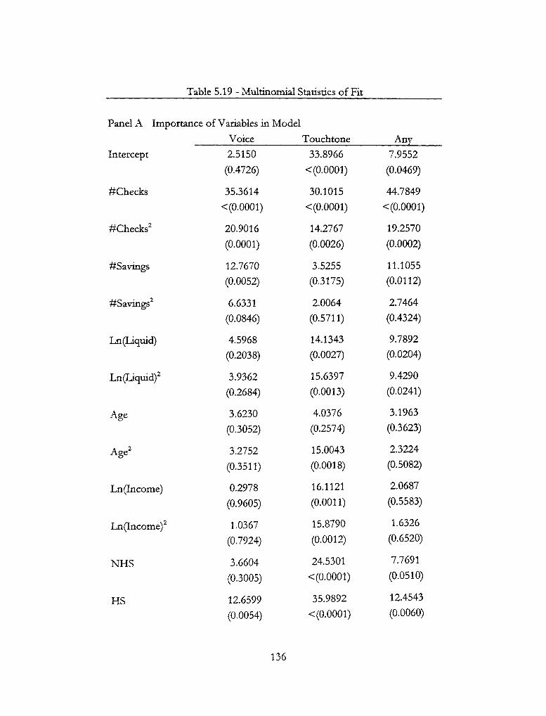
Table 5.19 - Multinomial Statistics of Fit
Panel A Importance
Intercept
#Checks
#Checks^
#Savings
#Savings^
Ln (Liquid)
Ln (Liquid)'
Age
Age'
Ln (Income)
Ln(Income)'
NHS
HS
of Variables in
Voice
2.5150
(0.4726)
35.3614
< (0.0001)
20.9016
(0.0001)
12.7670
(0.0052)
6.6331
(0.0846)
4,5968
(0.2038)
3.9362
(0.2684)
3.6230
(0.3052)
3.2752
(0.3511)
0.2978
(0.9605)
1,0367
(0,7924)
3.6604
(0.3005)
12.6599
(0.0054)
Model
Touchtone
33.8966
< (0.0001)
30.1015
< (0.0001)
14.2767
(0.0026)
3.5255
(0.3175)
2.0064
(0.5711)
14.1343
(0.0027)
15.6397
(0.0013)
4.0376
(0.2574)
15.0043
(0.0018)
16.1121
(0.0011)
15.8790
(0.0012)
24.5301
< (0.0001)
35.9892
< (0.0001)
Any
7.9552
(0.0469)
44.7849
< (0.0001)
19.2570
(0.0002)
11.1055
(0.0112)
2.7464
(0.4324)
9.7892
(0.0204)
9.4290
(0.0241)
3.1963
(0.3623)
2.3224
(0.5082)
2.0687
(0.5583)
1.6326
(0.6520)
7.7691
(0.0510)
12.4543
(0.0060)
136
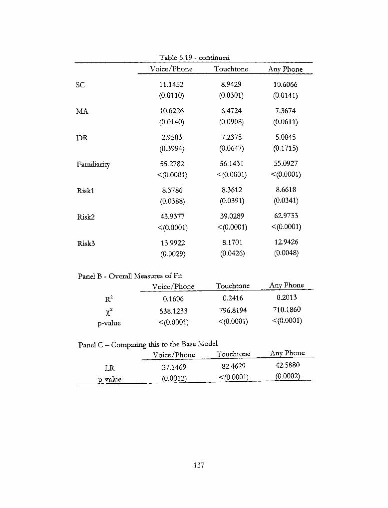
SC
MA
DR
FamiHarity
Riskl
Risk2
Risk3
Panel B
P-
- OveraU ]
R'
t -value
Table 5.19-
Voice/Phone
11.1452
(0.0110)
10.6226
(0.0140)
2.9503
(0.3994)
55.2782
< (0.0001)
8.3786
(0.0388)
43.9377
<(0.0001)
13.9922
(0.0029)
Measures of Fit
Voice/Phone
0.1606
538.1233
< (0.0001)
continued
Touchtone
8.9429
(0.0301)
6.4724
(0.0908)
7.2375
(0.0647)
56.1431
< (0.0001)
8.3612
(0.0391)
39.0289
<(0.0001)
8.1701
(0.0426)
Touchtone
0.2416
796.8194
< (0.0001)
Any Phone
10.6066
(0.0141)
7.3674
(0.0611)
5.0045
(0.1715)
55.0927
<(0.0001)
8.6618
(0.0341)
62.9733
< (0.0001)
12.9426
(0.0048)
Any Phone
0.2013
710.1860
<(0.0001)
Panel C - Comparing this to the Base Model Voice/Phone Touchtone Any Phone
LR
p-value
37.1469
(0.0012)
82.4629
< (0.0001)
42.5880
(0.0002)
137
Agaki panel B contains the test of Hypothesis 17 from Chapter 4. The overaU
models have prechctive power. Panel C compares the base to the squared multinomial logit
model. Using any definition of phone-banking, the squared model is superior to the base
model.
The tables that foUow in this section contain coefficient estimates for the individual
multinomial regressions and Wald statistics in parentheses. As was mentioned before, the
sample size of each outcome is important in interpreting tiie results. Going back to Table
5.1, one can see that by far the most popular outcome is conventional banking quadrant.
However, this outcome is the base. The next most popular is phone banking oiUy with a
sample size of more than 1,000. The two Intemet Banking outcomes are nearly equaUy
popular when defined as either voice or touchtone.
In the case of the voice phone-banking model (Table 5.20), the Internet only output
has few significant coefficients. None of tiie coefficients of utUity variables show any
statistical significance. And the only budget constrakit coefficients that are sigikficant are for
the dummy variables of education and for using other Intemet financial services. In
addition, the coefficients for the risk aversion dummy variables were also sigikficant.
It also is kiteresting to note that ki the model ki Table 5.20 the Hquid asset balance
variable is sigikficant ki distinguishing phone bank customers, whereas the kicome variable is
never significant. Again this variable is not knportant in choosing the Intemet, just the
phone-bankkig only outcome. It also is kiterestkig tiiat the Hquid asset balance squared term
is not significant, suggesting tiiat dimkkshkig marginal utihty is not experienced widi tiks
variable (altiiough this variable is akeady adjusted for dkiknishkig margkial utiHty by takkig
tiie natural log).
138
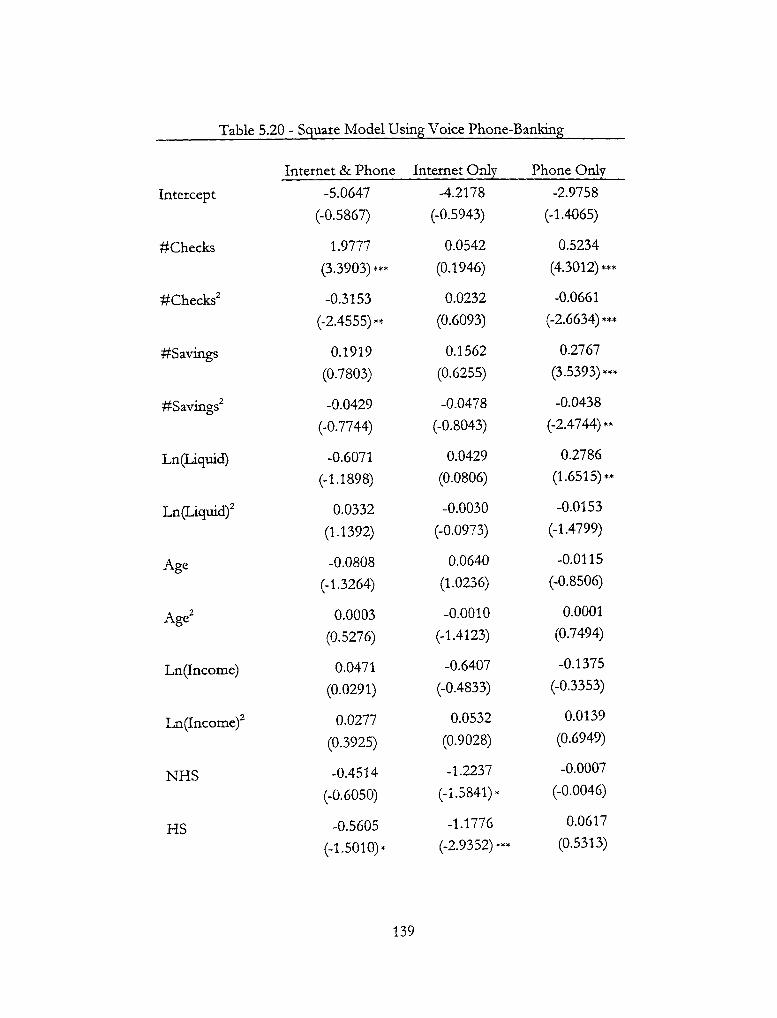
Table 5.20 - Square Model Using Voice Phone-Banking
Intercept
#Checks
#Checks'
#Savings
#Savings'
Ln (Liquid)
Ln(Liquid)'
Age
Age'
Ln(Income)
Ln (Income)'
NHS
HS
Internet & Phone
-5.0647
(-0.5867)
1.9777
(3.3903)***
-0.3153
(-2.4555)**
0.1919
(0.7803)
-0.0429
(-0.7744)
-0.6071
(-1.1898)
0.0332
(1.1392)
-0.0808
(-1.3264)
0.0003
(0.5276)
0.0471
(0.0291)
0.0277
(0.3925)
-0.4514
(-0.6050)
-0.5605
(-1.5010)*
Internet Only
-4.2178
(-0.5943)
0.0542
(0.1946)
0.0232
(0.6093)
0.1562
(0.6255)
-0.0478
(-0.8043)
0.0429
(0.0806)
-0.0030
(-0.0973)
0.0640
(1.0236)
-0.0010
(-1.4123)
-0.6407
(-0.4833)
0.0532
(0.9028)
-1.2237
(-1.5841)*
-1.1776
(-2.9352)***
Phone Only
-2.9758
(-1.4065)
0.5234
(4.3012)***
-0.0661
(-2.6634)***
0.2767
(3.5393)***
-0.0438
(-2.4744)**
0.2786
(1.6515)**
-0.0153
(-1.4799)
-0.0115
(-0.8506)
0.0001
(0.7494)
-0.1375
(-0.3353)
0.0139
(0.6949)
-0.0007
(-0.0046)
0.0617
(0.5313)
139
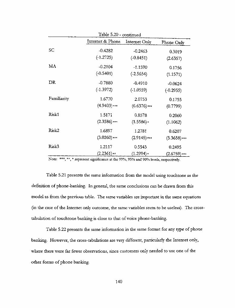
Table 5.20 - continued
SC
MA
DR
FamUiarity
Riskl
Risk2
Risk3
Internet &; Phone
-0.4282
(-1.2725)
-0.2104
(-0.5401)
-0.7880
(-1.3972)
1.6770
(4.9403)***
1.5171
(2.3586)-*-
1.6897
(3.0260)***
1.2117
(2.2361)**
Intemet Only
-0.2463
(-0.8451)
-1.1590
(-2.5654)
-0.4910
(-1.0559)
2.0753
(6.6376)***
0.8578
(1.5586)*
1.2781
(2.9145)***
0.5543
(1.2994)*
Phone Only
0.3019
(2.6357)
0.1756
(1.1571)
-0.0624
(-0.2955)
0.1755
(0.7799)
0.2060
(1.1062)
0.6207
(5.3658)***
0.2495
(2.6759)*** Note: ***, **, * represent significance at the 99%, 95% and 90% levels, respectively.
Table 5.21 presents the same information from the model using touchtone as the
defimtion of phone-banking. In general, the same conclusions can be drawn from this
model as from the previous table. The same variables are important in the same equations
(in the case of the Intemet only outcome, the same variables seem to be useless). The cross-
tabulation of touchtone banking is close to that of voice phone-banking.
Table 5.22 presents the same information in the same format for any type of phone
banking. However, tiie cross-tabulations are very different, particularly the Internet only,
where there were far fewer observations, since customers only needed to use one of the
other forms of phone banking.
140
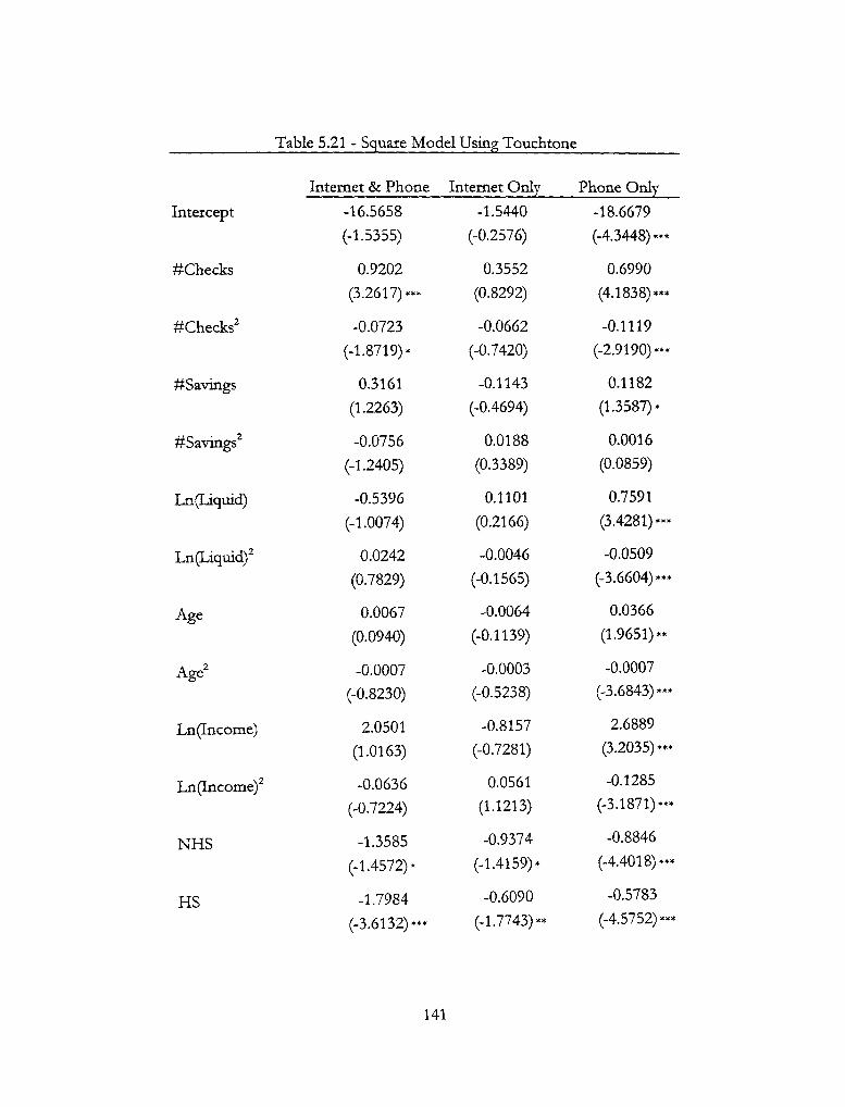
Table 5.21 - Square Model Using Touchtone
Intercept
#Checks
#Checks'
#Savings
#Savings'
Ln(Liquid)
Ln(Liquid)'
Age
Age'
Ln(Income)
Ln (Income)'
NHS
HS
Intemet & Phone
-16.5658
(-1.5355)
0.9202
(3.2617)***
-0.0723
(-1.8719)*
0.3161
(1.2263)
-0.0756
(-1.2405)
-0.5396
(-1.0074)
0.0242
(0.7829)
0.0067
(0.0940)
-0.0007
(-0.8230)
2.0501
(1.0163)
-0.0636
(-0.7224)
-1.3585
(-1.4572)*
-1.7984
(-3.6132)***
Intemet Only
-1.5440
(-0.2576)
0.3552
(0,8292)
-0.0662
(-0.7420)
-0.1143
(-0.4694)
0.0188
(0.3389)
0,1101
(0.2166)
-0.0046
(-0.1565)
-0.0064
(-0.1139)
-0.0003
(-0.5238)
-0.8157
(-0.7281)
0.0561
(1.1213)
-0.9374
(-1.4159)*
-0.6090
(-1.7743)**
Phone Only
-18.6679
(-4.3448)***
0.6990
(4.1838)***
-0.1119
(-2.9190)***
0.1182
(1.3587)*
0.0016
(0.0859)
0.7591
(3.4281)***
-0.0509
(-3.6604)***
0.0366
(1.9651)**
-0.0007
(-3.6843)***
2.6889
(3.2035)***
-0.1285
(-3.1871)***
-0.8846
(-4.4018)***
-0.5783
(-4.5752) ***
141
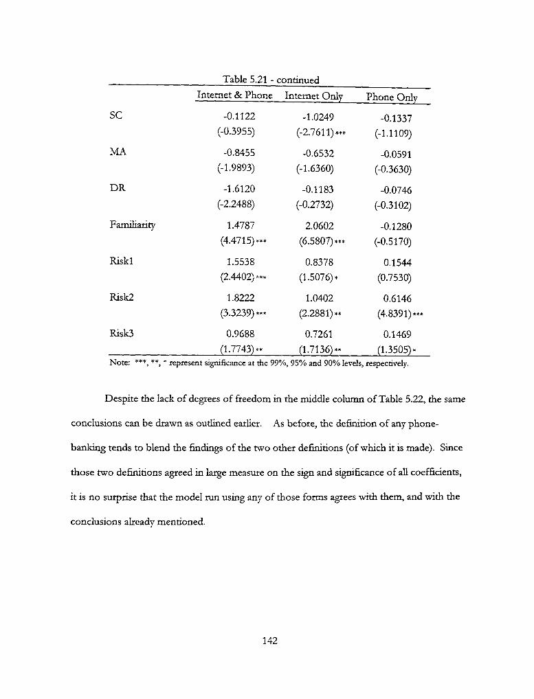
Table 5.21 - continued
SC
MA
DR
FamiHarity
Riskl
Risk2
Risk3
Intemet & Phone
-0.1122
(-0.3955)
-0.8455
(-1.9893)
-1.6120
(-2.2488)
1.4787
(4.4715)***
1.5538
(2.4402)***
1.8222
(3.3239)***
0.9688
(1.7743)**
Internet Only
-1.0249
(-2.7611)***
-0.6532
(-1.6360)
-0.1183
(-0.2732)
2.0602
(6.5807)***
0.8378
(1.5076)*
1.0402
(2.2881)**
0.7261
(1.7136)** ;nt significance at the 99%, 95% and 90% levels,
Phone Only ——— - -^
-0.1337
(-1.1109)
-0.0591
(-0.3630)
-0.0746
(-0.3102)
-0.1280
(-0.5170)
0.1544
(0.7530)
0.6146
(4.8391)***
0.1469
(1.3505)* , respectively.
Despite die lack of degrees of freedom in the midcUe column of Table 5.22, the same
conclusions can be ckawn as outhned earher. As before, the definition of any phone-
banking tends to blend the findings of the two other definitions (of which it is made). Since
those two definitions agreed in large measure on the sign and significance of aU coefficients,
it is no surprise that the model run using any of those forms agrees with them, and with the
conclusions aheady mentioned.
142
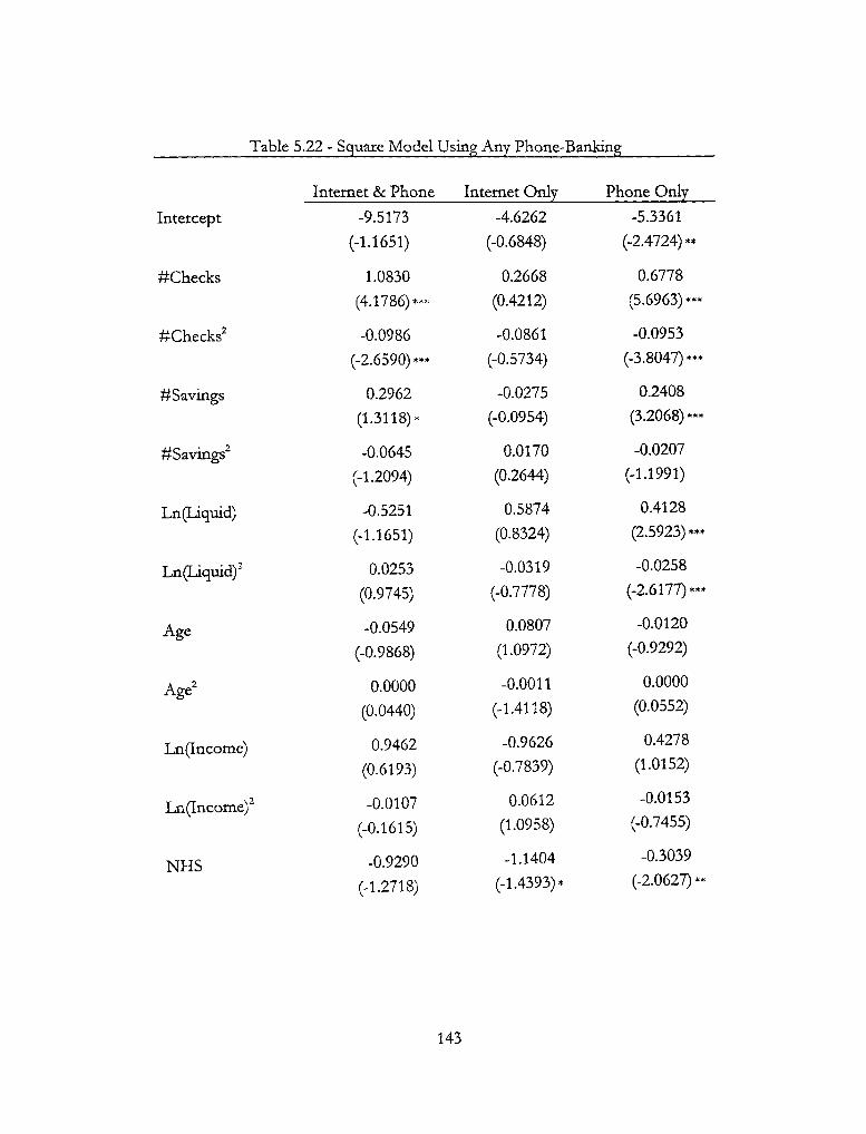
Table 5.22 - Square Model Using Any Phone-Banking
Intercept
#Checks
#Checks'
#Savings
#Savings'
Ln(Liqvkd)
Ln (Liquid)'
Age
Age'
Ln(lncome)
Ln (Income)"
NHS
Intemet & Phone
-9.5173
(-1.1651)
1.0830
(4.1786)***
-0.0986
(-2.6590)***
0.2962
(1.3118)*
-0.0645
(-1.2094)
-0.5251
(-1.1651)
0.0253
(0.9745)
-0.0549
(-0.9868)
0.0000
(0.0440)
0.9462
(0.6193)
-0.0107
(-0.1615)
-0.9290
(-1.2718)
Intemet Only
-4.6262
(-0.6848)
0.2668
(0.4212)
-0.0861
(-0.5734)
-0.0275
(-0.0954)
0.0170
(0.2644)
0.5874
(0.8324)
-0.0319
(-0.7778)
0.0807
(1.0972)
-0.0011
(-1.4118)
-0.9626
(-0.7839)
0.0612
(1.0958)
-1.1404
(-1.4393)*
Phone Only
-5.3361
(-2.4724)**
0.6778
(5.6963)***
-0.0953
(-3.8047)***
0.2408
(3.2068)***
-0.0207
(-1.1991)
0.4128
(2.5923)***
-0.0258
(-2.6177)***
-0.0120
(-0.9292)
0.0000
(0.0552)
0.4278
(1.0152)
-0.0153
(-0.7455)
-0.3039
(-2.0627)**
143
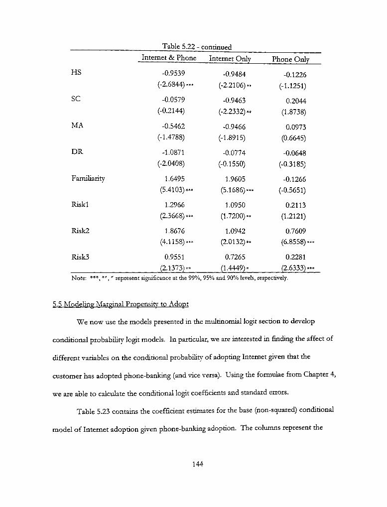
Table 5.22 - continued
HS
SC
MA
DR
Familiarity
Riskl
Risk2
Risk3
Intemet & Phone
-0.9539
(-2.6844)***
-0.0579
(-0.2144)
-0.5462
(-1,4788)
-1,0871
(-2.0408)
1.6495
(5.4103)***
1.2966
(2.3668)***
1.8676
(4.1158)***
0.9551
(2.1373)** ,t significance at the 99%,
Internet Only
-0.9484
(-2.2106)**
-0.9463
(-2.2332)**
-0.9466
(-1.8915)
-0.0774
(-0.1550)
1.9605
(5.1686)***
1.0950
(1.7200)**
1.0942
(2.0132)**
0.7265
(1.4449)* 95% and 90% levels.
Phone Only
-0.1226
(-1.1251)
0.2044
(1.8738)
0.0973
(0.6645)
-0.0648
(-0.3185)
-0.1266
(-0.5651)
0.2113
(1.2121)
0.7609
(6.8558) *«
0.2281
(2.6333)*** respectively.
5,5 ModeHng Marginal Propensity to Adopt
We now use the models presented in the multinomial logit section to develop
conditional probabihty logit models. In particular, we are interested in fincHng the affect of
different variables on the conditional probabUity of adopting Intemet given that tiie
customer has adopted phone-banking (and vice versa). Using the formulae from Chapter 4,
we are able to calculate the conchtional logit coefficients and sundard errors.
Table 5.23 contains die coefficient estimates for tiie base (non-squared) conditional
model of Intemet adoption given phone-bankkig adoption. The columns represent the
144

different defkktions of phone-bankkig. The statistics reported next to the description is the
coefficient estknate for tiie conditional logistic regression. The Wald statistic, reported ki
parentheses, tests whether the coefficient estimate is different from zero. It is knportant at
this juncture to remember the differences in observed remote banking outcomes.
From Table 5.23, it appears that the margkial propensity to adopt Intemet given
phone-banking depends on the number of checking accounts, age, income, education
(particularly some coUege and high school-whUe graduate degrees stiU appear to have the
wrong sign), famUiarit}'- with other Internet financial services, and risk aversion. These last
coefficients reject Hypothesis 17 from Chapter 4. The evidence suggests that bank
customers do perceive higher risk moving from phone- to Intemet banking, regardless of
how phone-banking is defined.
Because Intemet banking is so simUar to phone-banking in the services offered, it
would make sense that at least touchtone banking would not present any marginal risk
kicrease adopting phone-banking from Intemet banking, skice one interfaces only with a
computer. However, voice phone-banking may aUow people access to customer
kiformation or finances and could present an added perceived risk. To test for added
marginal risk, we calculate the conditional logistic regression coefficients for phone-banking
given Intemet banldng. The coefficient estimates and Wald statistics for the base model are
presented in Table 5.24.
The estimates ki Table 5.23 use tiie observations representing tiie outcomes Intemet
and phone-banking 2x16. phone-banking only. Togedier, tiiese estknates are based on weU over
1,000 observations (see Table 5.1). The conditional logistic regression ki Table 5.23 use far
fewer observations (only 163), and thereby has less power.
145
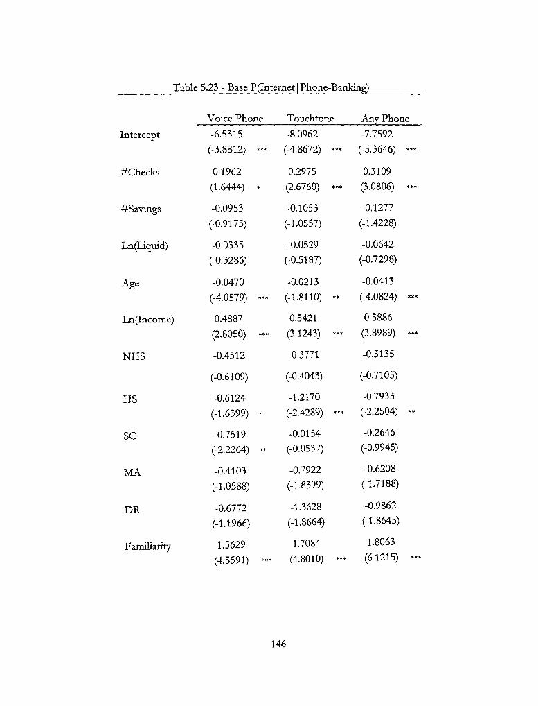
Table 5.23 - Base P(Intemet | Phone-Banking)
Intercept
#Checks
#Savings
Ln(Liquid)
Age
Ln(Income)
NHS
HS
SC
MA
DR
Familiarity
Voice Phone
-6.5315
(-3.8812) ***
0.1962
(1,6444) *
-0.0953
(-0.9175)
-0.0335
(-0.3286)
-0.0470
(-4.0579) ***
0.4887
(2.8050) ***
-0.4512
(-0.6109)
-0.6124
(-1.6399) *
-0.7519
(-2.2264) **
-0.4103
(-1.0588)
-0.6772
(-1.1966)
1.5629
(4.5591) ***
Touchtone
-8.0962
(-4.8672) ***
0.2975
(2.6760) ***
-0.1053
(-1.0557)
-0.0529
(-0.5187)
-0.0213
(-1.8110) **
0.5421
(3.1243) ***
-0.3771
(-0.4043)
-1.2170
(-2.4289) ***
-0.0154
(-0.0537)
-0.7922
(-1.8399)
-1.3628
(-1.8664)
1.7084
(4.8010) ***
Any Phone
-7.7592
(-5.3646) ***
0.3109
(3.0806) ***
-0.1277
(-1,4228)
-0.0642
(-0.7298)
-0.0413
(-4.0824) ***
0.5886
(3.8989) ***
-0.5135
(-0.7105)
-0.7933
(-2.2504) **
-0.2646
(-0.9945)
-0.6208
(-1.7188)
-0.9862
(-1.8645)
1.8063
(6.1215) ***
146
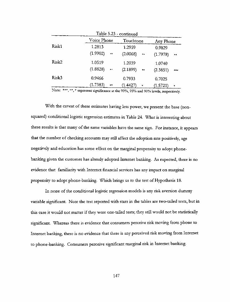
Table 5.23 - continued
Riskl
Risk2
Risk3
Voice Phone
1.2813
(1.9902)
1.0519
(1.8828)
0.9466
(1.7383)
**
**
**
Touchtone
1.2959
(2.0068)
1.2039
(2.1899)
0.7933
(1.4427)
**
**
*
Any Phone
0.9829
(1.7978) **
1.0740
(2.3851) ***
0.7025
(1.5721) * Note: ***, **, * represent significance at die 99%, 95% and 90% levels, respectively.
With the caveat of these estknates having less power, we present the base (non-
squared) conditional logistic regression estimates ki Table 24. What is kiteresting about
these results is that many of the same variables have the same sign. For instance, it appears
that the number of checking accounts may stiU affect the adoption rate positively, age
negatively and education has some effect on the marginal propensity to adopt phone-
banking given the customer has akeady adopted Intemet banldng. As expected, there is no
evidence that familiarity with Intemet financial services has any impact on marginal
propensitj' to adopt phone-banking. Which brings us to the test of Hypothesis 18.
In none of the conditional logistic regression models is any risk aversion dummy
variable significant. Note the test reported with stars in the tables are two-taUed tests, but in
this case it would not matter if they were one-taUed tests; they stUl would not be statisticaUy
significant. Whereas tiiere is evidence that consumers perceive risk moving from phone to
Intemet banking, there is no evidence that there is any perceived risk moving from Intemet
to phone-banking. Consumers perceive significant margkial risk in Intemet banking.
147
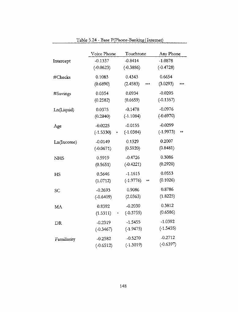
Table 5.24 - Base P(Phone-Bankkig | Intemet)
Intercept
#Checks
#Savings
Ln (Liquid)
Age
Ln(Income)
NHS
HS
SC
MA
DR
FamiHarity
Voice Phone
-0.1337
(-0.0623)
0.1083
(0.6890)
0.0354
(0.2582)
0.0375
(0.2840)
-0.0225
(-1.5330) *
-0.0149
(-0.0671)
0.5919
(0.5651)
0.5646
(1.0712)
-0.2693
(-0.6409)
0.8392
(1.5311) *
-0.2319
(-0.3467)
-0.2582
(-0.6512)
Touchtone
-0.8414
(-0.3886)
0.4343
(2.4583) ***
0.0934
(0.6659)
-0.1478
(-1.1084)
-0.0155
(-1.0384)
0.1329
(0.5920)
-0,4726
(-0,4221)
-1,1615
(-1.9776) **
0.9086
(2.0363)
-0.2030
(-0.3755)
-1.5455
(-1.9475)
-0.5270
(-1.3019)
Any Phone
-1.0878
(-0.4728)
0.6654
(3.0293) ***
-0.0205
(-0.1357)
-0.0976
(-0.6970)
-0.0299
(-1.9973) **
0.2007
(0.8481)
0.3086
(0.2920)
0.0553
(0.1026)
0.8786
(1.8225)
0.3812
(0.6586)
-1.0392
(-1.5455)
-0.2712
(-0.6397)
148
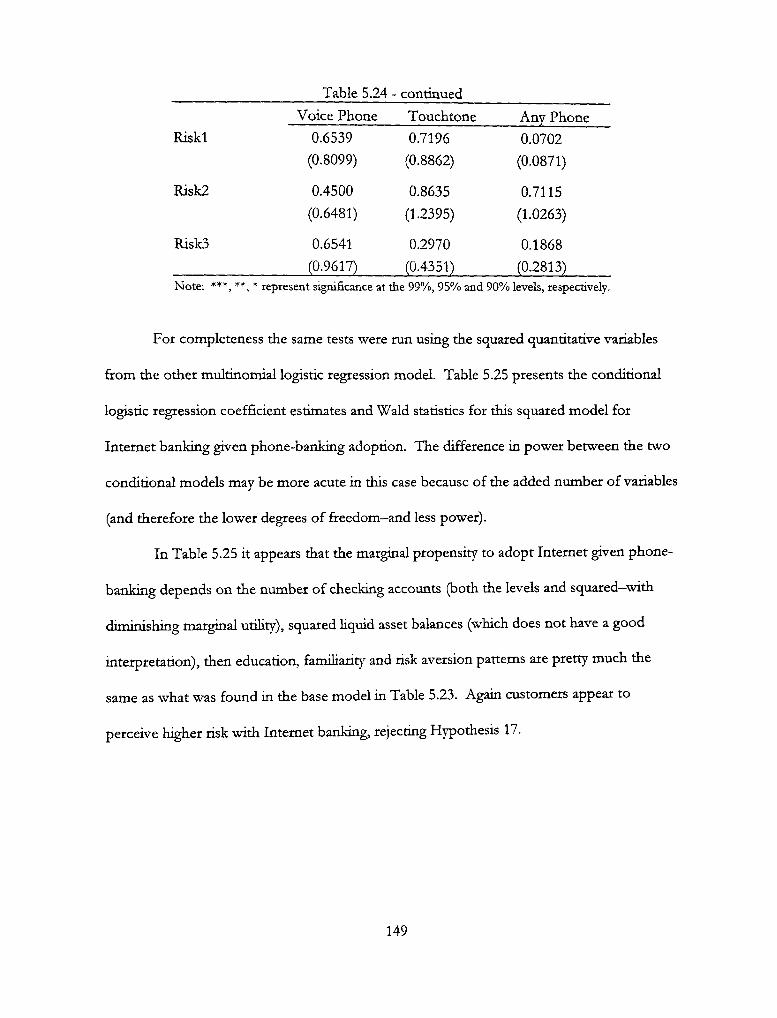
Table 5.24 - continued
Riskl
Risk2
Risk3
Voice Phone
0.6539
(0.8099)
0.4500
(0.6481)
0.6541
(0.9617)
Touchtone
0.7196
(0.8862)
0.8635
(1.2395)
0.2970
(0.4351)
Any Phone
0.0702
(0.0871)
0.7115
(1.0263)
0.1868
(0.2813) Note: ***, **, * represent significance at die 99%, 95% and 90% levels, respectively.
For completeness the same tests were run using the squared quantitative variables
from the other multinomial logistic regression model. Table 5.25 presents the conditional
logistic regression coefficient estimates and Wald statistics for this squared model for
Intemet banking given phone-banking adoption. The chfference in power between the two
conditional models may be more acute in tiks case because of the added nvimber of variables
(and therefore the lower degrees of freedom-and less power).
In Table 5.25 it appears that the margkial propensity to adopt Intemet given phone-
banking depends on the number of checking accounts (both the levels and squared-with
diminishing margkial utihty), squared Hquid asset balances (which does not have a good
interpretation), then education, famUiarity and risk aversion pattems are pretty much the
same as what was found ki die base model ki Table 5.23. Agaki customers appear to
perceive higher risk with Intemet bankkig, rejectkig Hj'pothesis 17.
149
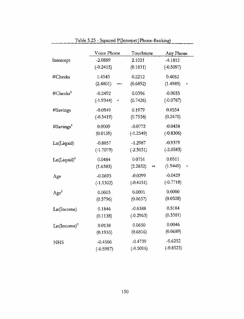
Table 5.25 - Squared P(Intemet j Phone-Banking)
Intercept
#Checks
#Checks'
#Savings
#Savings'
Ln (Liquid)
Ln(Liquid)'
Age
Age'
Ln(Income)
Ln(Income)"'
NHS
Voice Phone
-2.0889
(-0.2415)
1.4543
(2.4801) ***
-0.2492
(-1.9344) *
-0.0849
(-0.3419)
0.0009
(0.0159)
-0.8857
(-1.7079)
0.0484
(1.6383)
-0.0693
(-1.1302)
0.0003
(0.3796)
0.1846
(0.1138)
0.0138
(0.1955)
-0.4506
(-0.5987)
Touchtone
2.1021
(0.1831)
0.2212
(0.6892)
0.0396
(0.7426)
0.1979
(0.7558)
-0.0772
(-1.2549)
-1.2987
(-2.3031)
0.0751
(2.2832) **
-0.0299
(-0.4151)
0.0001
(0.0637)
-0.6388
(-0.2963)
0.0650
(0.6816)
-0.4739
(-0.5016)
Any Phone
-4.1812
(-0.5097)
0.4052
(1.4989) •
-0.0033
(-0.0787)
0.0554
(0.2470)
-0.0438
(-0.8306)
-0.9379
(-2.0583)
0.0511
(1.9449) *
-0.0429
(-0.7718)
0.0000
(0.0328)
0.5184
(0.3381)
0.0046
(0.0689)
-0.6252
(-0.8523)
150
Table 5.25 - continued
HS
SC
MA
DR
Voice Phone Touchtone Any Phone
FamUiarity
Riskl
Risk2
Risk3
-0.6222
(-1.6457)
-0.7301
(-2.1456)
-0.3860
(-0.9798)
-0.7256
(-1.2714)
1.5015
(4.3405)
1.3110
(2.0127)
1.0689
(1.9025)
0.9622
(1.7650)
-1.2202
(-2.4237) ***
0.0215
(0.0740)
-0.7864
(-1.8087)
-1.5374
(-2.0973)
1.6068
(4.4648) ***
1.3994
(2.1525) **
1.2076
(2.1820) **
0.8219
(1.4919) *
-0.8313
(-2.3411)
-0.2623
(-0.9788)
-0.6434
(-1.7542)
-1.0224
(-1.9274)
1.7761
(5.9653)
1.0853
(1.9731)
1.1068
(2.4397)
0.7270
(1.6221) Note: represent significance at the 99%, 95% and 90% levels, respectively.
Table 5.26 presents the conditional logistic regression coefficient estimates and Wald
statistics for the squared model of phone- given Intemet banking adoption. Possibly due to
the lower power discussed earher, tiks regression shows Httie affecting phone-banking
adoption, and may not be a fak test of Hypotiiesis 18. But again none of the risk aversion
variables show any statistical significance. There is stiU no evidence of perceived marginal
risk change moving from Intemet to phone-banking.
151
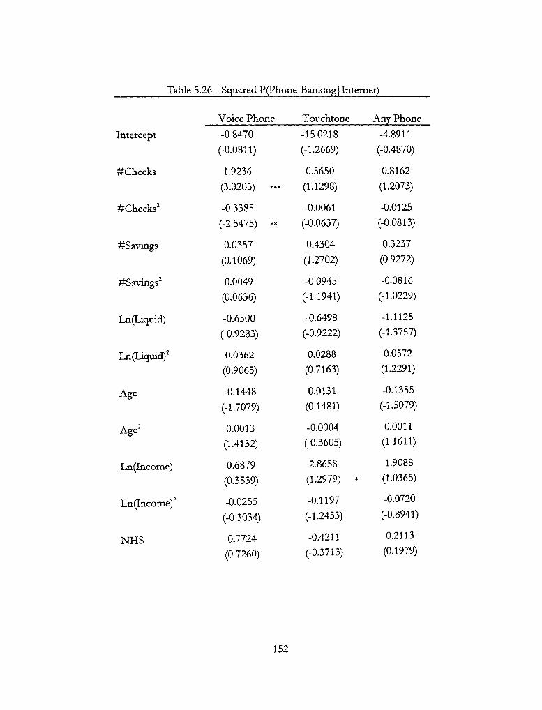
Table 5.26 - Squared P(Phone-Banking | Intemet)
Intercept
#Checks
#Checks'
#Savkigs
#Savkigs'
Ln(Liquid)
Ln (Liquid)'
Age
Age'
Ln(Income)
Ln (Income)'
NHS
Voice Phone
-0.8470
(-0.0811)
1.9236
(3.0205) ***
-0.3385
(-2.5475) **
0.0357
(0.1069)
0.0049
(0.0636)
-0.6500
(-0.9283)
0.0362
(0.9065)
-0.1448
(-1.7079)
0.0013
(1.4132)
0.6879
(0.3539)
-0.0255
(-0.3034)
0.7724
(0.7260)
Touchtone
-15.0218
(-1.2669)
0.5650
(1.1298)
-0.0061
(-0.0637)
0.4304
(1.2702)
-0.0945
(-1.1941)
-0.6498
(-0.9222)
0.0288
(0.7163)
0.0131
(0.1481)
-0.0004
(-0.3605)
2.8658
(1.2979) *
-0.1197
(-1.2453)
-0.4211
(-0.3713)
Any Phone
-4.8911
(-0.4870)
0.8162
(1.2073)
-0.0125
(-0.0813)
0.3237
(0.9272)
-0.0816
(-1.0229)
-1.1125
(-1.3757)
0.0572
(1.2291)
-0.1355
(-1.5079)
0.0011
(1.1611)
1.9088
(1.0365)
-0.0720
(-0.8941)
0.2113
(0.1979)
152
Table 5.26 - continued
Voice Phone
HS
SC
MA
DR
Touchtone Any Phone
Familiarity
Riskl
Risk2
Risk3
0.6171
(1.1579)
-0.1819
(-0.4274)
0.9486
(1.6969)
-0.2970
(-0.4389)
-0.3983
(-0.9875)
0.6592
(0.8051)
0.4116
(0.5878)
0.6574
(0.9618)
-1.1894
(-2.0116)
0.9127
(2.0324)
-0.1923
(-0.3517)
-1.4937
(-1.8802)
-0.5814
(-1.4263)
0.7161
(0.8737)
0.7820
(1.1119)
0.2426
(0.3540)
-0.0055
(-0.0102)
0.8884
(1.8352)
0.4004
(0.6843)
-1.0097
(-1.4953)
-0.3110
(-0.7280)
0.2016
(0.2485)
0.7734
(1.1096)
0.2285
(0.3429) Note: ***, **, * represent significance at the 99%, 95% and 90% levels, respectively.
5.6 AUowing Subjective Probability to Vary
Up untU now, we have assumed that aU customers have identical subjective
probabihty sets. We wUl now test to see if subjective probabUities do in fact vary. For this
section, only the Internet banking adoption is interesting. There were two models presented
in Section 4.6, depending on how risk was modeled. We demonstrated in Section 5.2 that
Intemet bankkig can be modeled uskig only one risk variable, the numbered response from
the survey (1, 2, 3 or 4-representkig levels of kicreaskig risk aversion), which greatiy
153
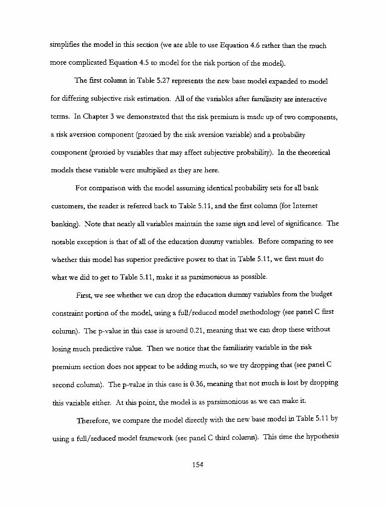
sknphfies the model in this section (we are able to use Equation 4.6 rather than the much
more comphcated Equation 4.5 to model for the risk portion of the model).
The fijist column in Table 5.27 represents the new base model expanded to model
for differing subjective risk estimation. AU of the variables after familiarity are interactive
terms. In Chapter 3 we demonstrated that the risk premium is made up of two components,
a risk aversion component (proxied by the risk aversion variable) and a probabUity
component (proxied by variables that may affect subjective probabihty). In the theoretical
models these variable were multiphed as they are here.
For comparison with the model assuming identical probabihty sets for aU bank
customers, the reader is referred back to Table 5.11, and the first colurrm (for Intemet
banking). Note that nearly aU variables maintain the same sign and level of significance. The
notable exception is that of aU of the education dummy variables. Before comparing to see
whether this model has superior predictive power to that in Table 5.11, we first must do
what we did to get to Table 5.11, make it as parsimonious as possible.
Fkst, we see whether we can drop the education dummy variables from the budget
constrakit portion of the model, using a fuU/reduced model methodology (see panel C first
column). The p-value ki this case is around 0.21, meankig that we can chop these without
losing much predictive value. Then we notice that the famUiarity variable ki the risk
premium section does not appear to be addkig much, so we try droppkig that (see panel C
second column). Tlie p-value ki this case is 0.36, meankig tiiat not much is lost by droppkig
this variable either. At this pokit, the model is as parsimonious as we can make it.
Therefore, we compare the model dkecdy witii tiie new base model ki Table 5.11 by
uskig a foU/reduced model framework (see panel C tiikd column). This time die hypodiesis
154

tiiat tiie predictive value is the same for botii models is actuaUy rejected at die 0.05 level that
we have been uskig duroughout tiks tiiesis. That means tiiat tiie model that assumes varying
subjective probabUity estimates is a better predictor. In particular, education and age appear
to affect the subjective probabiht)^ of customers adoptkig the internet.
It is important to note that the signs and significance of aU other variables seem
vmaffected by this new model. In addition, aU of the education interactive variables have the
correct sign. The one puzzle is that the age interaction variable does not have the
h}'pothesized sign.
It is assumed that as one gets older, one would be less likely to adopt Intemet
banking, due to lack of experience with tiie technology, etc. In adchtion the higher the risk
aversion variable gets, the higher the level of risk aversion. In other words, both of these
variables should be negatively related to Intemet banking adoption. When multiphed
together, one wovdd think the coefficient shovUd be negative. But this is an interaction
variable, where the expected sign is unclear and the overaU effect even more unclear. The
coefficient is statisticaUy significant, but its effect only can be seen via a graph which
highhghts the variables in question, age and risk aversion.
Figure 5.1 shows the interaction between age and risk. The y-axis is the value of the
Logit function:
i-\-e
where L= the hnear combination impHed by the regression output.
The X-axis is the subject's response to the risk aversion survey question (1, 2, 3, 4-increaskig
levels of risk aversion).
155
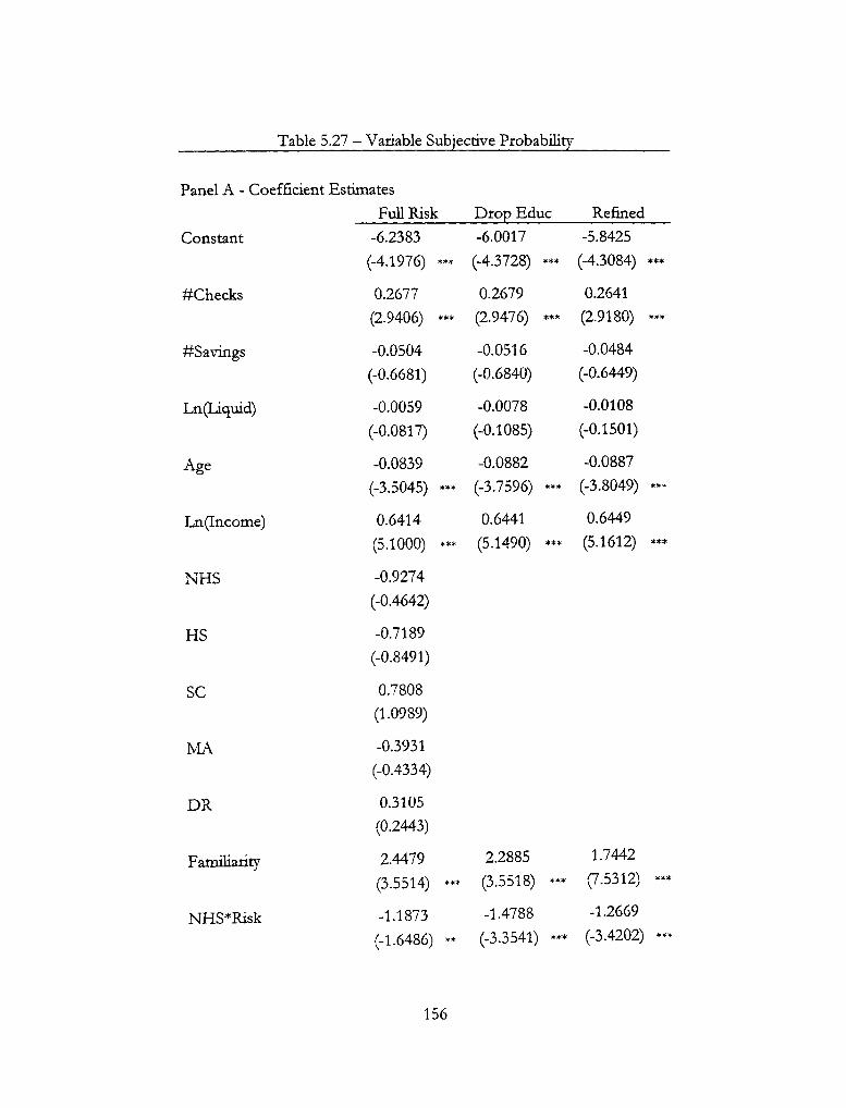
Table 5.27 - Variable Subjective ProbabUity
Panel A - Coefficient Estimates
Constant
#Checks
#Savings
Ln(Liquid)
Age
Ln(Income)
NHS
HS
SC
MA
DR
FamUiarity
NHS*Risk
FuU Risk
-6.2383
(-4.1976) **-
0.2677
(2.9406) ***
-0.0504
(-0.6681)
-0.0059
(-0.0817)
-0.0839
(-3.5045) •**
0.6414
(5.1000) ***
-0.9274
(-0.4642)
-0.7189
(-0.8491)
0.7808
(1.0989)
-0.3931
(-0.4334)
0.3105
(0.2443)
2.4479
(3.5514) ***
-1.1873
(-1.6486) **
Drop Educ
-6.0017
(-4.3728) ***
0.2679
(2.9476) ***
-0.0516
(-0.6840)
-0.0078
(-0.1085)
-0.0882
(-3.7596) ***
0.6441
(5.1490) ***
2.2885
(3.5518) ***
-1.4788
(-3.3541) ***
Refined
-5.8425
(-4.3084) ***
0.2641
(2.9180) ***
-0.0484
(-0.6449)
-0.0108
(-0.1501)
-0.0887
(-3.8049) ***
0.6449
(5.1612) ***
1.7442
(7.5312) ***
-1.2669
(-3.4202) ***
156
Table 5.27 - continued
HS*Risk
SC*Risk
BA*Risk
MA*Risk
DR*Risk
Age*Risk
(FamUiarity-1) *Risk
FuU Risk
-1.2082
(-2.5669)
-1.5907 (-3.5841)
-1.1061 (-2.5689)
-1.2273 (-2.4075)
-1.4743 (-2.2711)
0.0167 (2.1069)
0.3218 (1.0480)
***
***
***
***
*.*
***
Drop Educ
-1.4687
(-3.5197)
-1.3425 (-3.2782)
-1.1350 (-2.7706)
-1.4107 (-3.3639)
-1.3796 (-3.1857)
0.0182 (2.3352)
0.2624 (0.8999)
***
***
***
***
***
***
Refined
-1.2571 (-3.6770) ***
-1.1368 (-3.3786) ***
-0.9326 (-2.7511) -**
-1.2066 (-3.4477) ***
-1.1762 (-3.2082) ***
0.0184 (2.3755) ***
Panel B - Statistics of Fit Expanded Drop Educ Refined
R'
l' p-value
0.2339
276.49 <0.0001
0.2384
282.03 <0.0001
0.2377
281.20 <0.0001
Panel C - Likelihood Ratios
Drop Educ Refined Risky-Riskp
Ukehhood Ratio 9.5736 0.8284 4.7067
p-value 0.2141 0.3627 0.0300
Note: ***, **, * represent significance at die 99%, 95% and 90% levels, respectively.
157
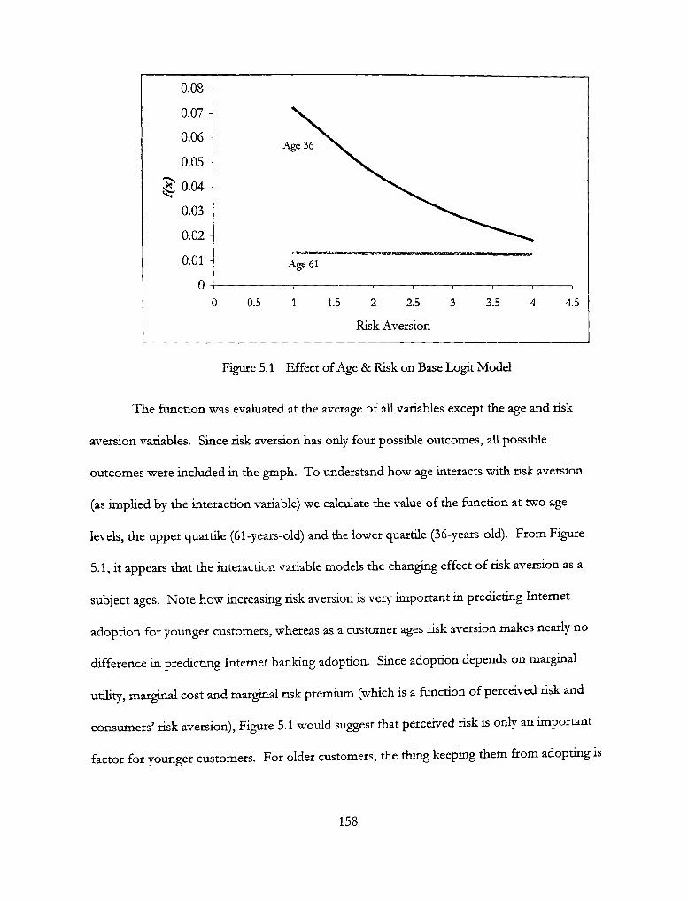
Figure 5.1 Effect of Age & Risk on Base Logit Model
The fvmction was evaluated at the average of aU variables except the age and risk
aversion variables. Since risk aversion has only four possible outcomes, aU possible
outcomes were kicluded in the graph. To understand how age interacts with risk aversion
(as imphed by the interaction variable) we calculate the value of the function at two age
levels, the upper quartile (61-years-old) and the lower quartUe (36-years-old). From Figure
5.1, it appears that the kiteraction variable models the changkig effect of risk aversion as a
subject ages. Note how kicreaskig risk aversion is very important ki predicting Intemet
adoption for younger customers, whereas as a customer ages risk aversion makes nearly no
difference ki predictkig Internet bankkig adoption. Skice adoption depends on margkial
utihtjr, margkial cost and margkial risk premium (which is a function of perceived nsk and
consumers' risk aversion). Figure 5.1 would suggest tiiat perceived risk is only an knportant
factor for younger customers. For older customers, die tiikig keepkig tiiem from adopting is
158

die marginal utiHty gaki vis-a-vis tiie margkial cost. For tiiem die margkial cost, which may
kiclude trainkig and the purchase of a computer, is greater than the margkial benefit.
But what is most kiterestkig is tiiat tiie risk aversion variable should pick up the
sensitivity to perceived risk (or its knportance ki die decision to adopt). From the evidence
m Figure 5.1, die perceived risk of the Intemet appears to be an knportant decision variable
only for the younger customers.
We now analyze the knpact of these fkidkigs on the multkiomial output as weU as
the margkial propensity to adopt. This tkne we wiU not consider aU possible configvurations;
we wiU only consider two: the base model and the squared model. The base varying
perceived risk model wUl be a multkiomial model as set forth in Table 5.27. The squared
model wiU add squared variables for the first five variables in that Hst. We wiU consider the
base model first.
Table 5.28 presents the overaU statistics of fit for the base multinomial model. Again
the columns represent the (hfferent definitions of phone-banking. Panel A shows the
significance of each variable throughout the model (how much prechctabUity is lost by
dropping it from the model). The value in parentheses is the p-value. Most of the variables
maintain the same sign and significance as noted earher. It is noteworthy that the Hquid
assets variable is stUl not important. But also noteworthy is the fact that the Risk*Age
variable needed in the bivariate logistic regression is not needed in the multinomial
regression. AU education based risk premium variables are significant.
Panel B shows the overaU significance of the model, which is significant for aU
models run.
159
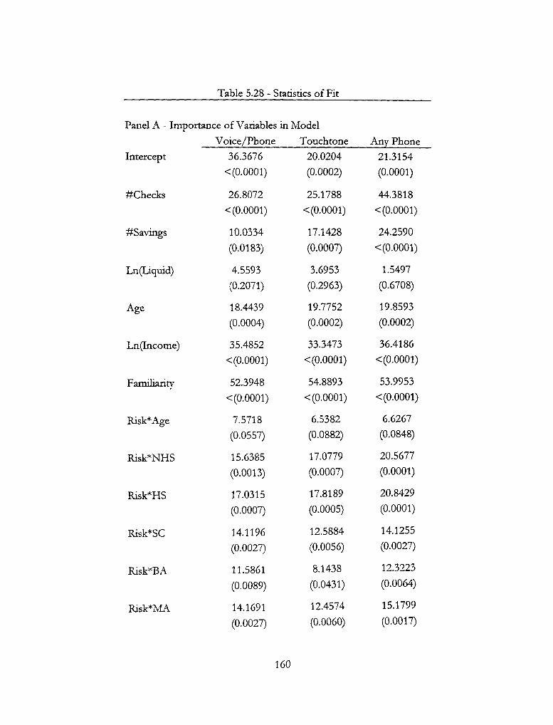
Table 5.28 - Statistics of Fk
Panel A Importance of Variables in Model
Intercept
#Checks
#Savings
Ln (Liquid)
Age
Ln(lncome)
Familiarity
Risk* Age
Risk*NHS
Risk*HS
Risk*SC
Risk*BA
Risk*MA
Voice/Phone
36.3676
<(0.0001)
26.8072
< (0.0001)
10.0334
(0.0183)
4.5593
(0.2071)
18.4439
(0.0004)
35.4852
<(0.0001)
52.3948
< (0.0001)
7.5718
(0.0557)
15.6385
(0.0013)
17.0315
(0.0007)
14.1196
(0.0027)
11.5861
(0.0089)
14.1691
(0.0027)
Touchtone
20.0204
(0.0002)
25.1788
<(0.0001)
17.1428
(0.0007)
3.6953
(0.2963)
19.7752
(0.0002)
33.3473
<(0.0001)
54.8893
<(0.0001)
6.5382
(0.0882)
17.0779
(0.0007)
17.8189
(0.0005)
12.5884
(0.0056)
8.1438
(0.0431)
12.4574
(0.0060)
Any Phone
21.3154
(0.0001)
44.3818
< (0.0001)
24.2590
< (0.0001)
1.5497
(0.6708)
19.8593
(0.0002)
36.4186
< (0.0001)
53.9953
< (0.0001)
6.6267
(0.0848)
20.5677
(0.0001)
20.8429
(0.0001)
14.1255
(0.0027)
12.3223
(0.0064)
15.1799
(0.0017)
160
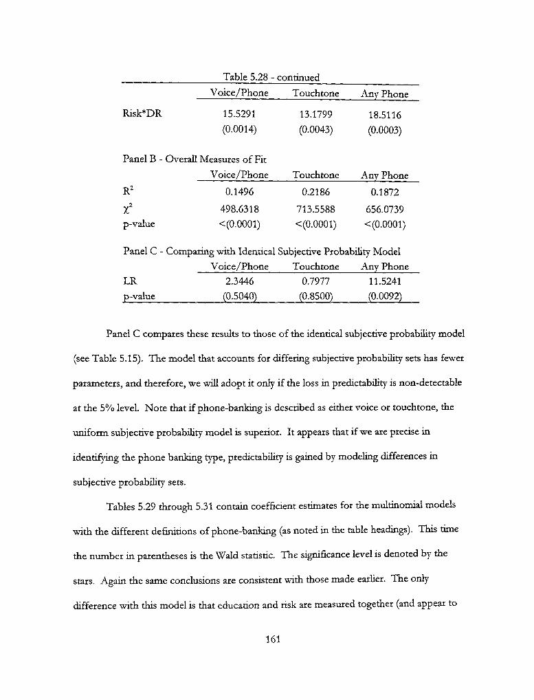
Table 5.28 - continued
Risk*DR
Panel B -
R'
t p-value
Voice/Phone
15.5291
(0.0014)
OveraU Measures of Fit
Voice/Phone
0.1496
498.6318
<(0.0001)
Touchtone
13.1799
(0.0043)
Touchtone
0.2186
713.5588
<(0.0001)
Any Phone
18.5116
(0.0003)
Any Phone
0.1872
656.0739
<(0.0001)
Panel C - Comparing with Identical Subjective Probabihty Model
Voice/Phone Touchtone Any Phone
LR 2.3446 0.7977 11.5241
p-value (0.5040) (0.8500) (0.0092)
Panel C compares these results to those of the identical subjective probabihty model
(see Table 5.15). The model that accounts for cHffering subjective probabihty sets has fewer
parameters, and therefore, we wiU adopt it only if the loss in prechctabUity is non-detectable
at the 5% level. Note that if phone-banking is described as either voice or touchtone, the
uniform subjective probabihty model is superior. It appears that if we are precise in
identifying the phone bankkig type, prechctabUity is gakied by modeHng differences ki
subjective probabihty sets.
Tables 5.29 through 5.31 contain coefficient estknates for the multinomial models
with the different definitions of phone-bankkig (as noted in the table headings). This tkne
the number ki parentheses is the Wald statistic. The significance level is denoted by the
stars. Agaki the same conclusions are consistent with those made earher. The only
(Hfference with tiks model is that education and risk are measured together (and appear to
161

better capture the risk premium in most instances than the model assuming uniform
subjective probabihties with three different levels of risk measured as a dummy variable).
These multinomial logistic regressions imply conditional coefficients Hke those
presented in Table 5.22 and 5.23. For the base varying perceived risk model, these estimates
are found in Tables 5.32 and 5.33. These coefficients measure the effect of each variable on
the marginal propensity to adopt Intemet banldng given phone-banking adoption or vice
versa. The figvires in parentheses are the Wald statistics for each coefficient
Table 5.32 presents the coefficient estimates for calculating the probabUity of
adopting Intemet banking given phone-banking. In aU cases the education level risk
premium variables are statisticaUy significant and the Risk^Age variable is positive (as noted
before in the bivariate estimates). AU other variables are consistent with the uniform
subjective probabUity estimates. The conclusions under varying perceived risk estimates is
the same as it was before, that perceived risk matters (as does nvimber of checkkig accounts,
income, age, and famiHarity with other forms of electronic financial services).
Table 5.33 presents the coefficient estimates for calculating the probabUity of
adoptkig phone-bankkig given Intemet bankkig. Unhke the identical subjective probabUity
models, some of diese variables are statisticaUy significant. Particularly kiteresting is tiie
doctorate variable that is significant under die voice phone model and not under die umform
perceived risk model, su^esting tiiat tiiose witii doctoral degrees perceive a different kkid of
risk movkig from Intemet to voice phone-bankkig (which is possible smce tiiey may present
uniquely different risks).
162
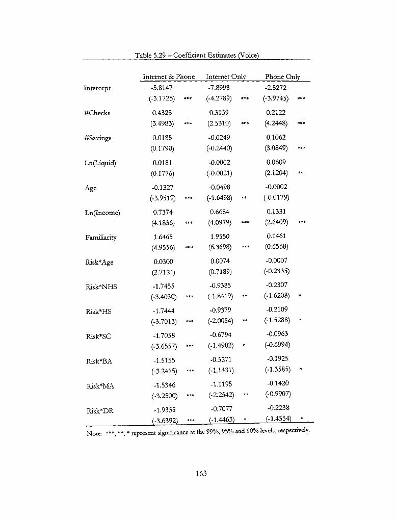
Table 5.29 - Coefficient Estimates (Voice)
Intercept
#Checks
#Savings
Ln (Liquid)
Age
Ln (Income)
FamiHarity
Risk*Age
Risk*NHS
Risk*HS
Risk*SC
Risk*BA
Risk*MA
Risk*DR
Note: ***, **, * rep
Internet & Phone
-5.8147
(-3.1726)
0.4325
(3.4983)
0.0185
(0.1790)
0.0181
(0.1776)
-0.1327
(-3.9519)
0.7374
(4.1836)
1.6465
(4.9556)
0.0300
(2.7124)
-1.7455
(-3.4030)
-1.7444
(-3.7013)
-1.7058
(-3.6557)
-1.5155
(-3.2415)
-1.5346
(-3.2500)
-1.9335
(-3.6392)
iresent significar
***
* * • *
***
* * * •
***
***
***
***
V * *
***
* • *
ice at 1
Intemet Only
-7.8998
(-4.2789)
0.3139
(2.5310)
-0.0249
(-0.2440)
-0.0002
(-0.0021)
-0.0498
(-1.6498)
0.6684
(4.0979)
1.9550
(6.3698)
0.0074
(0.7189)
-0.9385
(-1.8419)
-0.9379
(-2.0054)
-0.6794
(-1.4902)
-0.5271
(-1.1431)
-1.1195
(-2.2542)
-0.7077
(-1,4463)
***
***
**
***
***
**
**
*
**
*
Phone Only
-2.5272
(-3.9745) ***
0.2122
(4.2448) ***
0.1062
(3.0849) ***
0,0609
(2,1204) **
-0,0002
(-0,0179)
0.1331
(2.6409) ***
0.1461
(0.6568)
-0.0007
(-0.2335)
-0.2307
(-1.6208) *
-0.2109
(-1.5288) *
-0.0963
(-0.6994)
-0.1925
(-1.3585) *
-0.1420
(-0.9907)
-0.2238
(-1.4554) *
the 99%, 95% and 90% levels, respectively.
163
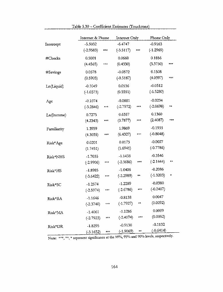
Table 5.30 - Coefficient Estimates (Touchtone)
Intercept
#Checks
#Savings
Ln(Iiquid)
Age
Ln(Income)
Famiharit)'
Risk* Age
Risk-^'NHS
Risk^HS
Risk*SC
Risk*BA
Risk*MA
Risk*DR
Note: ***,**,
Intemet & Phone
-5.5032
(-2.9583)
0.5001
(4.4565)
0.0578
(0.5903)
-0.1049
(-1.0373)
-0.1074
(-3.2846)
0.7275
(4.2343)
1.3959
(4.3035)
0.0201
(1.7451)
-1.7035
(-2,9906)
-1,8985
(-3.6422)
-1.2574
(-2.5974)
-1.1646
(-2.3740)
-1.4061
(-2.7923)
-1.8295
(-3.1652)
* represent significani
***
***
***
***
***
**+
* • *
***
***
***
Intemet Only
-6.4747
(-3.5117)
0.0660
(0.4330)
-0.0572
(-0.5187)
0.0536
(0.5551)
-0.0881
(-2.7972)
0.6357
(3.7877)
1.9869
(6.4327)
0.0173
(1.6941)
-1.1438
(-2.3686)
-1.0406
(-2.2989)
-1.2289
(-2.6786)
-0.8138
(-1.7927)
-1.1286
(-2.4074)
***
***
***
***
***
**
***
**
***
-0.9130
*** (-1.9069) **
ce at die 99%, 95% and 90%
Phone Only
-0.9163
(-1.2969)
0.1856
(3.3750) ***
0.1508
(4.0397) ***
-0.0512
(-1.5280)
-0.0234
(-2.0698) **
0.1360
(2.4087) ***
-0.1955
(-0.8048)
-0.0027
(-0.7786)
-0.3546
(-21444) **
-0.2086
(-1.3203) *
-0.0380
(-0.2407)
0.0047
(0.0292)
0.0009
(0.0052)
-0.1132
(-0.6414)
levels, respectively.
164
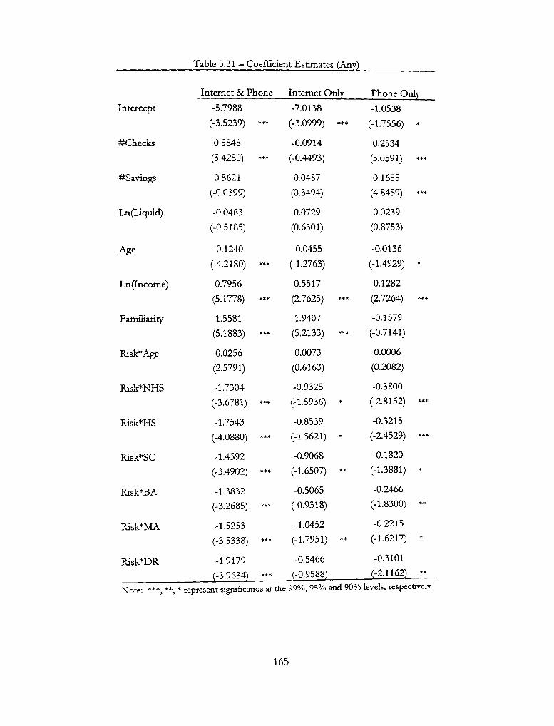
Table 5.31 - Coefficient Estimates (Any)
Intercept
#Checks
#Savings
Ln (Liquid)
Age
Ln(Income)
FamiHarity
Risk* Age
Risk*NHS
Risk*HS
Risk*SC
Risk*BA
Risk*MA
Risk*DR
Note: ***, **, * re
Internet & Phone
-5.7988
(-3.5239)
0.5848
(5.4280)
0.5621
(-0.0399)
-0.0463
(-0.5185)
-0.1240
(-4.2180)
0.7956
(5.1778)
1.5581
(5.1883)
0.0256
(2.5791)
-1,7304
(-3,6781)
-1,7543
(-4,0880)
-1.4592
(-3.4902)
-1,3832
(-3.2685)
-1.5253
(-3.5338)
-1.9179
(-3.9634)
***
***
***
***
***
***
¥ * *
***
***
***
**.*
:present significance at t
Intemet Only
-7.0138
(-3.0999)
-0.0914
(-0.4493)
0.0457
(0.3494)
0.0729
(0.6301)
-0.0455
(-1.2763)
0.5517
(2.7625)
1.9407
(5.2133)
0.0073
(0.6163)
-0.9325
(-1.5936)
-0.8539
(-1.5621)
-0.9068
(-1.6507)
-0.5065
(-0.9318)
-1.0452
(-1.7951)
-0.5466
***
***
***
*
*
*«
**
(-0.9588)
•he 99%, 95% and 90°/
Phone Only
-1.0538
(-1.7556) *
0.2534
(5.0591) ***
0.1655
(4.8459) ***
0.0239
(0.8753)
-0.0136
(-1.4929) *
0.1282
(2.7264) ***
-0.1579
(-0.7141)
0.0006
(0.2082)
-0.3800
(-2.8152) ***
-0.3215
(-2.4529) ***
-0.1820
(-1.3881) *
-0.2466
(-1.8300) **
-0.2215
(-1.6217) *
-0.3101
(-2.1162) **
0 levels, respectively.
165
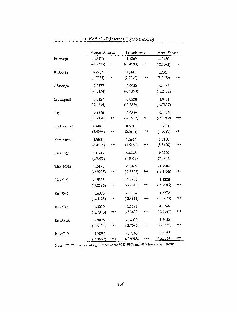
Table 5.32 - P(Intemet|Phone-Bankmg)
Intercept
#Checks
#Savings
Ln (Liquid)
Age
Ln (Income)
Familiarity
Risk* Age
Risk*NHS
Risk*HS
Risk*SC
Risk*BA
Risk*MA
Risk*DR
Voice Phone
-3.2875 (-1.7735)
0.2203 (1.7984)
-0.0877 (-0,8434)
-0,0427 (-0.4144)
-0.1326 (-3.9178)
0,6043 (3,4038)
1,5004 (4.4114)
0,0306 (2,7506)
-1.5148 (-2.9223)
-1,5335 (-3,2186)
-1,6095 (-3.4128)
-1.3230 (-2.7973)
-1.3926 (-2,9171)
-1,7097 (-3.1857)
*
**
***
y * *
***
***
***
* • * *
***
***
***
Touchtone -4.5869 (-2,4190)
0,3145 (2,7940)
-0,0930 (-0.9390)
-0.0538 (-0,5224)
-0,0839 (-2,5252)
0,5915 (3,3902)
1,5914 (4,5166)
0,0228 (1,9518)
-1,3489 (-2,3365)
-1,6899 (-3,2015)
-1,2194 (-2.4836)
-1,1693 (-2,3499)
-1,4070 (-2,7546)
-1,7163 (-2,9288)
**
***
***
***
***
***
***
***
***
***
***
Any Phone
-4,7450 (-2,9042) ***
0,3314 (3,2172) ***
-0,1143 (-1,2752)
-0,0701 (-0,7877)
-0,1105 (-3,7769) ***
0,6674 (4,3621) ***
1,7160 (5,8406) '**
0,0250 (2,5283)
-1,3504 (-2,8756) ***
-1,4328 (-3,3505) ***
-1,2772 (-3,0673) ***
-1,1366 (-2,6967) ***
-1,3038 (-3,0335) ***
-1,6078 (-3,3334) ***
Note: , : 4 i « * H-* * represent significance at the 99%, 95% and 90% levels, respectively.
166
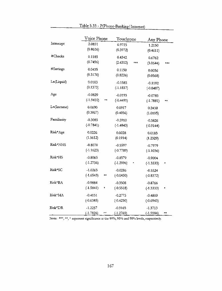
Intercept
#Checks
#Savings
Ln (Liquid)
Age
Ln(Income)
Familiarity
Risk* Age
Risk*NHS
Risk*HS
Risk*SC
Risk*BA
Risk*MA
Risk*DR
Note* *** ** •
Voice Phone 2.0851
(0.8616)
0.1185
(0.7456)
0.0435
(0.3170)
0.0183
(0.1373)
-0,0829
(-1.9410)
0,0690
(0,3067)
-0,3085
(-0.7841)
0,0226
(1,5612)
-0,8070
(-1,1623)
-0,8065
(-1,2736)
-1,0263
(-1,6543)
-0,9884
(-1,5841)
-0,4151
(-0,6385)
-1,2257
(-1,7826)
**
**
^
**
Touchtone 0,9715
(0,3972)
0,4342
(2,4312) ***
0,1150
(0,8226)
-0,1585
(-1,1837)
-0,0193
(-0,4491)
0,0917
(0,4056)
-0,5910
(-1,4843)
0,0028
(0,1914)
-0,5597
(-0,7789)
-0,8579
(-1,2996) *
-0,0286
(-0,0450)
-0,3508
(-0,5518)
-0,2775
(-0,4250)
-0,9165
(-1,2769)
'• represent significance at the 99%, 95% and 90% levels
Any Phone 1.2150
(0.4611)
0.6762
(3.0644) ***
0.0056
(0,0368)
-0,1192
(-0,8487)
-0.0785
(-1.7881) **
0,2438
(1.0195)
-0,3826
(-0,9144)
0,0183
(1,2329)
-0,7979
(-1,1036)
-0,9004
(-1,3533) *
-0,5524
(-0,8372)
-0,8766
(-1,3333) *
-0,4800
(-0,6943)
-1,3713
(-1,9184) **
, respectively.
167

Agaki we investigate the effect of the kiteraction tean Age*Risk. Figures 5.2-5.4
show the effect of age and risk on the probabUity of Intemet adoption given that different
forms of phone banking have been adopted. In aU cases, we see the same general
relationship we saw in Figure 5.1. As customers age, the effect of thek risk aversion is not
only tempered, but seems to reverse. It seems that if an older customer has adopted phone
bankkig, lower risk is perceived ki Internet banking. For aU younger customers, Intemet
adoption is seen as increasing thek perceived risk.
Figures 5.5-5.7 show the effect of age and risk on the probabUity of different types
of phone banking adoption given Intemet banking adoption. This is where being precise in
the type of phone banking makes a difference in the interpretation. Figure 5.5 shows the
effect of age and risk aversion on voice phone banking given Intemet bankkig. Notice how
older customers perceive less risk adopting phone banking given they have akeady adopted
Intemet banking, possibly representing an after hours avenue of help if they make a mistake
online. At the same time, younger customers perceive greater risk in adopting phone
banking, possibly representing the added risk of aUowing other people (phone bank workers)
access to your personal financial information.
Figure 5.6 shows the effect of age and risk on the probabihty of touchtone banking
given Intemet bankkig adoption. In this instance, risk aversion has ahnost no effect on
phone banking adoption. If anytiikig, there is less risk perceived (possibly due to the fact
that one can fix any problems caused by one via the other). The same results can be seen ki
Figure 5.7, which represents the effect of age and risk on the probabUity of any type of
phone banking given Intemet banking adoption.
168
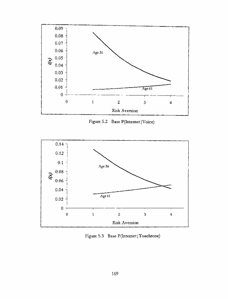
Figure 5.2 Base P(Intemet | Voice)
Figure 5.3 Base P(Intemet |Touchtone)
169
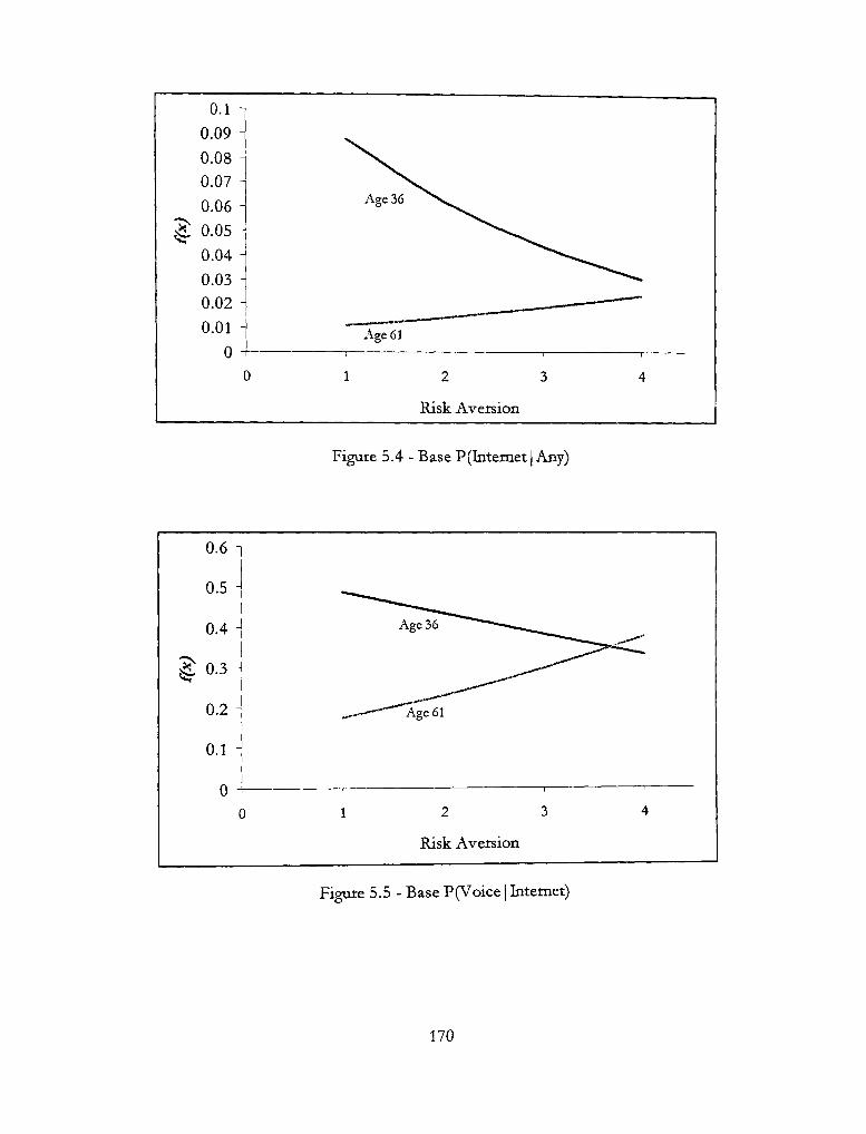
2 3
Risk Aversion
Figure 5.4 - Base P(Intemet | Any)
Figure 5.5 - Base P(Voice | Intemet)
170
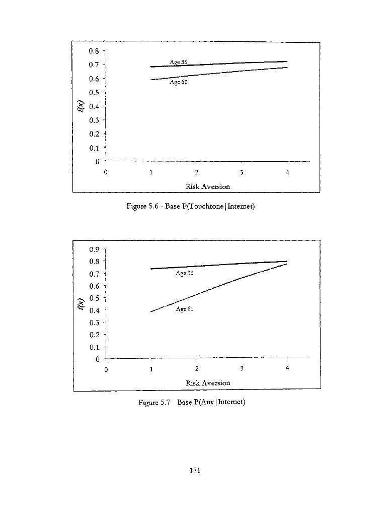
Figure 5.6 - Base P(Touchtone | Intemet)
Figure 5.7 Base P(Any | Intemet)
171
We now tum our attention to tiie squared model. Under the identical subjective
probabUity model, this model was found to be the most predictive/parsknonious (although
sometknes more difficult to interpret). We begin ovur discussion with Table 5.34 which
presents the overaU statistics of fit. Remember that the columns represent the different
definitions of phone-bankkig. Again panel A shows the significance of each variable
throughout the model (how much predictabUity is lost by dropping it from the model). The
value in parenthesis is the p-value. Except for the changed variables aU coefficient estknates
maintain the same sign and significance as under the uniform perceived risk model. Unlike
the base model presented on the previous several pages, the Risk^Age variable is a significant
predictor. And AU education based risk premium variables are significant.
Panel B shows the overaU significance of the model, which is significant for aU
models run.
Panel C compares these results to those of the identical perceived risk model (see
Table 5.19). The varying perceived risk model has fewer parameters, and therefore, we wUl
adopt it only if the loss in predictabihty is non-detectable at the 5% level (we are looking for
p-values greater than 5%). l ike the base model, as long as we specificaUy define phone-
banking, the varying perceived risk model is superior. If phone-banking is described as
either voice or touchtone, the uniform perceived risk model is superior.
Panel D compares these results to those of the base varying perceived risk model
(see table 5.28). Skice the squared model has more parameters to estknate, we should only
choose it if its predictive power is greater. The p-values show that in aU cases, this model is
superior to that of the base model (we are lookkig for p-values less than 5%). From that
criteria, tiks is the best model.
172
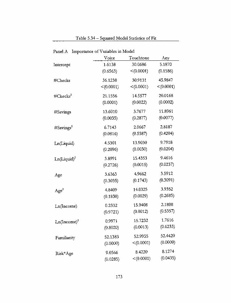
Table 5.34 - Squared Model Statistics of Fit
Panel A Importance c
Intercept
#Checks
#Checks'
#Savings
#Savings'
Ln(Liquid)
Ln (Liquid)'
Age
Age'
Ln (Income)
Ln (Income)'
Famiharit}^
Risk* Age
)f Variables in
Voice
1.6138
(0.6563)
36.1238
<(0.0001)
21.1556
(0.0001)
13.6010
(0.0035)
6.7143
(0.0816)
4.5301
(0.2096)
3.8991
(0.2726)
3.6363
(0.3035)
4.8409
(0.1838)
0.2332
(0.9721)
0.9971
(0,8020)
52,1383
(0.0000)
9.0566
(0.0285)
Model
Touchtone
30.0686
<(0.0001)
30.9131
<(0.0001)
14.5577
(0.0022)
3.7677
(0.2877)
2.0667
(0.5587)
13.9030
(0.0030)
15.4353
(0.0015)
4.9662
(0.1743)
14.0325
(0.0029)
15.9408
(0.0012)
15.7232
(0.0013)
52.9955
<(0.0001)
8.4220
<(0.0001)
Any
5.1870
(0.1586)
45.9847
<(0.0001)
20.0168
(0.0002)
11.8961
(0.0077)
2.8187
(0.4204)
9.7918
(0.0204)
9.4616
(0.0237)
3.5912
(0.3091)
3.9352
(0.2685)
2.1808
(0.5357)
1.7616
(0.6233)
52.4420
(0.0000)
8.1274
(0.0435)
173
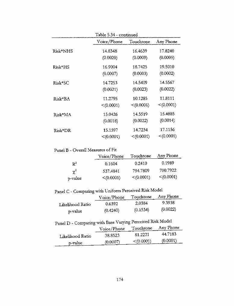
Table 5.34 - continued
Risk*NHS
Risk*HS
Risk*SC
Risk*BA
Risk*^LA.
Risk*DR
Voice/Phone
14.8348
(0.0020)
16.9004
(0.0007)
14.7253
(0.0021)
11.2795
< (0.0001)
15.0426
(0.0018)
15.1597
<(0.0001)
Touchtone
16.4639
(0.0009)
18.7425
(0.0003)
14.5409
(0.0023)
10.1285
< (0.0001)
14.5519
(0.0022)
14.7234
<(0.0001)
Any Phone
17.8240
(0.0005)
19.5010
(0.0002)
14.5567
(0.0022)
11.8111
< (0.0001)
15.4885
(0.0014)
17.1156
<(0.0001)
Panel B - OveraU Measures of Fit
Voice/Phone
R'
t p-value
0.1604
537.4841
< (0.0001)
Touchtone Any Phone
0.2410 0.1989
794.7809 700.7922
< (0,0001) < (0.0001)
Panel C - Comparing with Uniform Perceived Risk Model
Voice/Phone Touchtone Any Phone
likehhood Ratio 0.6392 2.0384 9.3938 p-value (0.4240) (0.1534) (0.0022)
Panel D - Comparing witii Base Varykig Perceived Risk Model Voice/Phone Touchtone Any Phone
44.7183 likelihood Ratio
p-value
38.8523
(0.0007)
81.2221
< (0.0001) (0.0001)
174
For completeness, we kiclude die parameter estimates of this multinomial logistic
regression. Tables 5.35 tiirough 5.37 present tiie coefficient estimates for tiuree models,
dependkig on die definition of phone-bankkig (see tiie headkig for each table). Each table
contakis die coefficient estknate, witii the Wald statistic ki parentheses. The level of
significance is denoted by die number of stars. Most variables tiiat are common to the
uniform perceived risk models and varykig perceived risk models can be kiterpreted the
same. Therefore the analysis from the earher section stUl holds. Some squared terms change
from being insignificant to significant with this latest model.
There is a subtie difference in how perceived risk is modeled between the umform
and varying perceived risk models. In the uniform perceived risk model, risk aversion is an
important predictor variable of the onljphone-banking outcome. In Tables 5.35 and 5.36,
none of the risk premium variables (not even the Risk*Age with the wrong sign) are
sigmficant in predicting the only phone-banking outcome. Some of these variables appear to be
important in Table 5.37, but that model is neither precise nor the best model (using a
fuU/reduced model mediodology—the uniform perceived risk model is better). From this
evidence, it would appear that a good level of predictabUity is lost in imprecisely defining
phone-banking.
As in the base case, we now tum to the impHed conditional probabihty models (the
marginal propensity to adopt). The result of this analysis is found in Tables 5.38 and 5.39.
The table reports the estimated effect of one variable on the conditional probabihty, with the
Wald statistic in parentheses. The significance level is noted by the number of stars next to
the Wald statistic.
175
These estimates contain some kiteresting findings. Considering the probabUity of
adopting Intemet bankkig given phone-bankkig (Table 5.38), tiie risk premium variables are
unsurprisingly important ki predictimg Internet bankkig adoption given phone-bankkig
adoption. Also the famiHarity with other electronic fkiancial services is a strong predictor.
What is surpriskig is ki the case of touchtone banking (and the any designation), the Hquid
assets variable is negative, as predicted if the customer is fearfiil of losing money through
unauthorized access. And vmder touchtone banking, no utiHty variables are positive,
suggestkig that httie utiHty is added by Intemet bankkig (at least through the variables in our
model).
Considering the probabihty of adopting phone-banking given Intemet bankkig
(Table 5.39), nearly the same conclusions can be drawn as noted in the uniform perceived
risk models. It is interesting that those with doctoral degrees, considering adopting voice
banking would be found to perceive some risk if our significance level were 10%. This is an
interesting finding because, as was noted in the uniform perceived risk models, the sample
size in this case is much smaUer than that of Table 5.38, and that outcome would be
consistent with the base model findings in Table 5.33.
For completeness, at the end of the tables, the same graphs (Tables 5.10-5.15) are
generated as were generated for the base model. These analyze the net effect of risk on the
adoption probabUity. Although the graphs are not as clear, the same conclusions can be
drawn. The only oddity is that in aU kistances of Intemet adoption given phone bankkig
function, the probabUity kicreases even for younger people as one's risk aversion moves
from 1 to 2.
176
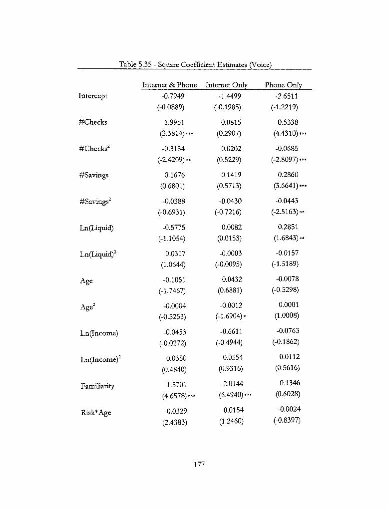
Table 5.35 - Square Coefficient Estimates (Voice)
Intercept
#Checks
#Checks'
#Savings
#Sa\Tngs'
Ln (Liquid)
Ln (liquid)'
Age
Ln(Income)
Ln(Income)'
FamUiarity
Risk* Age
Intemet & Phone
-0.7949
(-0.0889)
1.9951
(3.3814)***
-0.3154
(-2.4209)**
0.1676
(0.6801)
-0.0388
(-0.6931)
-0.5775
(-1.1054)
0.0317
(1.0644)
-0.1051
(-1.7467)
-0.0004
(-0.5253)
-0.0453
(-0.0272)
0.0350
(0.4840)
1.5701
(4.6578)***
0.0329
(2.4383)
Intemet Only
-1.4499
(-0.1985)
0.0815
(0.2907)
0.0202
(0.5229)
0.1419
(0.5713)
-0.0430
(-0.7216)
0.0082
(0.0153)
-0.0003
(-0.0095)
0.0432
(0.6881)
-0.0012
(-1.6904)*
-0.6611
(-0.4944)
0.0554
(0.9316)
2.0144
(6.4940)***
0.0154
(1.2460)
Phone Only
-2.6511
(-1.2219)
0.5338
(4.4310)***
-0.0685
(-2.8097)***
0.2860
(3.6641)***
-0.0443
(-2.5163)**
0.2851
(1.6843)**
-0.0157
(-1.5189)
-0.0078
(-0.5298)
0.0001
(1.0008)
-0.0763
(-0.1862)
0.0112
(0.5616)
0.1346
(0.6028)
-0.0024
(-0.8397)
177
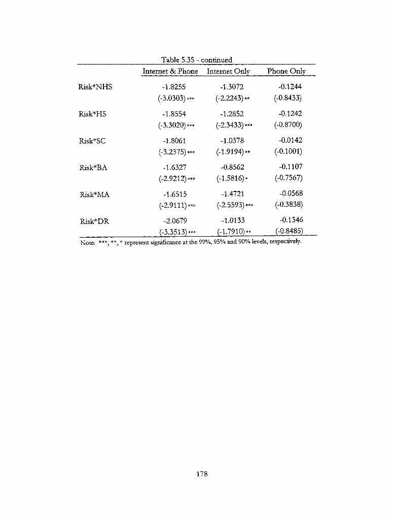
Table 5,35 - continued
Risk*NHS
Risk*HS
Risk*SC
Risk*BA
Risk*MA
Risk*DR
Internet & Phone
-1,8255
(-3,0303) «**
-1.8554
(-3.3020)***
-1,8061
(-3,2375)***
-1,6327
(-2.9212)***
-1.6515
(-2.9111)***
-2.0679
(-3.3513)***
Intemet Only
-1.3072
(-2.2243)**
-1.2852
(-2.3433)***
-1.0378
(-1.9194)**
-0.8562
(-1.5816)*
-1.4721
(-2.5593)***
-1.0133
(-1.7910)**
Phone Only
-0.1244
(-0.8433)
-0.1242
(-0.8700)
-0.0142
(-0.1001)
-0.1107
(-0.7567)
-0.0568
(-0.3838)
-0.1346
(-0.8485)
Note: ***, **, * represent significance at the 99%, 95% and 90% levels, respectively.
178
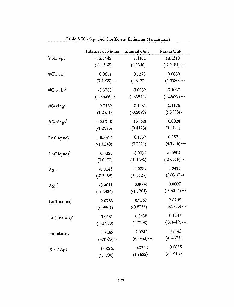
Table 5.36 - Squared Coefficient Estimates (Touchtone)
Intercept
#Checks
#Checks'
#Savings
#Savings'
Ln(Liquid)
Ln (Liquid)'
Age
Age'
Ln(Income)
Ln (Income)'
FamUiarity
Risk*Age
Intemet & Phone
-12.7442
(-1.1362)
0.9611
(3.4039)***
-0.0765
(-1.9666)**
0.3169
(1.2351)
-0.0748
(-1.2175)
-0.5517
(-1.0240)
0.0251
(0.8072)
-0.0243
(-0.3455)
-0.0011
(-1.2886)
2.0753
(0.9961)
-0.0631
(-0.6950)
1.3658
(4.1893)***
0.0262
(1.8798)
Internet Only
1.4402
(0.2340)
0.3373
(0.8132)
-0.0589
(-0.6944)
-0.1481
(-0.6079)
0.0250
(0.4473)
0.1157
(0.2271)
-0.0038
(-0.1290)
-0.0289
(-0.5127)
-0.0008
(-1.1701)
-0.9267
(-0.8238)
0.0638
(1.2708)
2.0242
(6.5353)***
0.0222
(1.8682)
Phone Only
-18.1310
(-4.2181)***
0.6880
(4.2380)***
-0.1087
(-2.9587)***
0.1175
(1.3553)*
0.0028
(0.1494)
0.7521
(3.3945)***
-0.0504
(-3.6319)***
0.0413
(2.0318)**
-0.0007
(-3.3214)***
2.6208
(3.1700)***
-0.1247
(-3.1412)**-
-0.1145
(-0.4673)
-0.0035
(-0,9107)
179
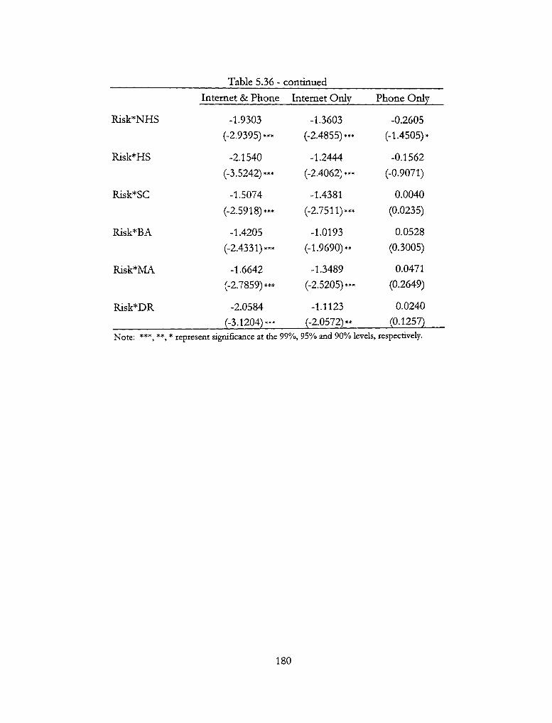
Table 5.36 - continued
Risk*NHS
Risk*HS
Risk*SC
Risk*BA
Risk*MA
Risk*DR
Intemet & Phone
-1.9303
(-2.9395)***
-2.1540
(-3.5242)***
-1.5074
(-2.5918)***
-1.4205
(-2.4331)***
-1.6642
(-2.7859)***
-2.0584
(-3.1204)***
Intemet Only
-1.3603
(-2.4855)***
-1.2444
(-2.4062)***
-1.4381
(-2.7511)***
-1.0193
(-1.9690)**
-1.3489
(-2.5205)***
-1.1123
(-2.0572)**
Phone Only
-0.2605
(-1.4505)*
-0.1562
(-0.9071)
0.0040
(0.0235)
0.0528
(0.3005)
0.0471
(0.2649)
0.0240
(0.1257)
Note: ***, **, * represent significance at die 99%, 95% and 90% levels, respectively.
180
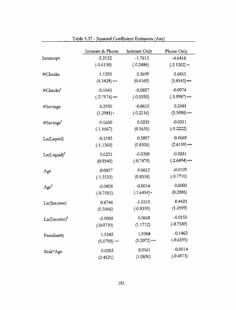
Table 5.37 - Squared Coefficient Estimates (Any)
Intercept
#Checks
#Checks'
#Savkigs
#Savings'
Ln(Liquid)
Ln(Liquid)'
Age
Age'
Ln (Income)
Ln(Income)'
Familiarity
Risk*Age
Intemet & Phone
-5.2132
(-0.6150)
1.1293
(4.3428)***
-0.1045
(-2.7974)***
0.2930
(1.2981)*
-0.0630
(-1.1667)
-0.5183
(-1.1360)
0.0251
(0.9540)
-0.0857
(-1.5533)
-0.0005
(-0.7581)
0.8746
(0.5566)
-0.0050
(-0,0730)
1,5342
(5,0798)***
0.0285
(2.4521)
Intemet Only
-1.7612
(-0.2486)
0.2699
(0.4169)
-0.0857
(-0.5550)
-0.0610
(-0.2116)
0.0235
(0.3635)
0.5897
(0.8306)
-0.0308
(-0.7470)
0.0612
(0.8318)
-0.0014
(-1.6454)*
-1.0515
(-0.8359)
0.0668
(1.1712)
1.9504
(5.2072)-**
0.0161
(1.0830)
Phone Only
-4.6418
(-2.1202)**
0.6855
(5.8543)***
-0.0974
(-3.9987)***
0.2481
(3.3088)***
-0.0211
(-1.2222)
0.4169
(2.6159)***
-0.0261
(-2.6494) ***
-0.0109
(-0.7710)
0.0000
(0.2886)
0.4423
(1.0599)
-0.0155
(-0.7589)
-0.1462
(-0.6595)
-0.0014
(-0.4973)
181
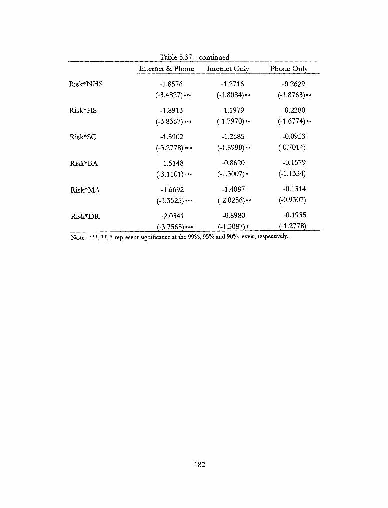
Table 5.37 - continued
Risk*NHS
Risk*HS
Risk*SC
Risk*BA
Risk*MA
Risk*DR
Intemet & Phone
-1.8576
(-3.4827)***
-1.8913
(-3.8367)***
-1.5902
(-3.2778)***
-1.5148
(-3.1101)***
-1.6692
(-3.3525)***
-2.0341
(-3,7565)***
Intemet Only
-1.2716
(-1.8084)**
-1.1979
(-1.7970)**
-1.2685
(-1.8990)**
-0.8620
(-1.3007)*
-1.4087
(-2.0256)**
-0.8980
(-1.3087)*
Phone Only
-0.2629
(-1.8763)**
-0.2280
(-1.6774)**
-0.0953
(-0.7014)
-0.1579
(-1.1334)
-0.1314
(-0.9307)
-0.1935
(-1.2778)
Note: ***, **, * represent significance at die 99%, 95% and 90% levels, respectively.
182
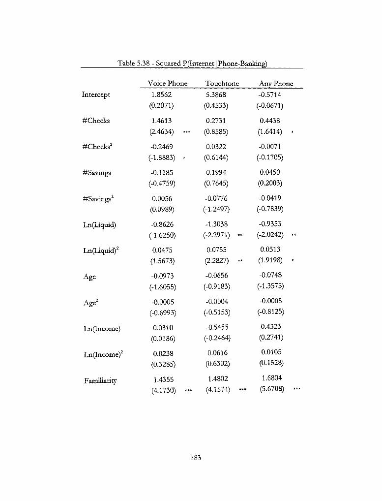
Table 5.38 - Squared P(Intemet | Phone-Banking)
Intercept
#Checks
#Checks'
#Savings
#Savkigs'
Ln(Liquid)
Ln(Liquid)'
Age
Age'
Ln(Income)
Ln(Income)
FamiHarity
Voice Phone
1.8562
(0.2071)
1.4613
(2.4634) ***
-0.2469
(-1.8883) *
-0.1185
(-0.4759)
0.0056
(0.0989)
-0.8626
(-1.6250)
0.0475
(1.5673)
-0.0973
(-1.6055)
-0.0005
(-0.6993)
0.0310
(0.0186)
0.0238
(0.3285)
1.4355
(4.1730) ***
Touchtone
5.3868
(0.4533)
0.2731
(0.8585)
0.0322
(0.6144)
0.1994
(0.7645)
-0.0776
(-1.2497)
-1.3038
(-2.2971) **
0.0755
(2.2827) **
-0.0656
(-0.9183)
-0.0004
(-0.5153)
-0.5455
(-0.2464)
0.0616
(0.6302)
1.4802
(4.1574) ***
Any Phone
-0.5714
(-0.0671)
0.4438
(1.6414) *
-0.0071
(-0.1705)
0.0450
(0.2003)
-0.0419
(-0.7839)
-0.9353
(-2.0242) **
0.0513
(1.9198) *
-0.0748
(-1.3575)
-0.0005
(-0.8125)
0.4323
(0.2741)
0.0105
(0.1528)
1.6804
(5.6708) ***
183
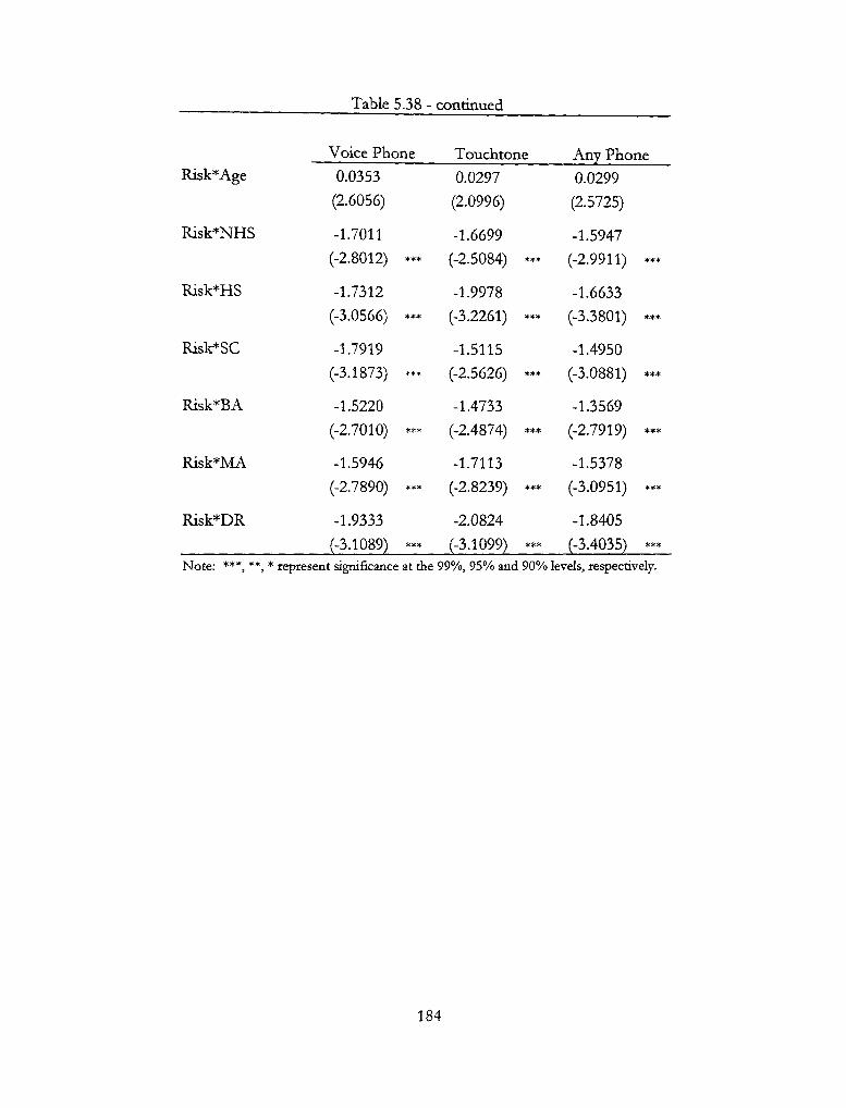
Table 5.38 - contkiued
Risk* Age
Risk*NHS
Risk*HS
Risk*SC
Risk*BA
Risk*MA
Risk*DR
Note: ***, **, * repi
Voice Phone
0.0353
(2.6056)
-1.7011
(-2.8012)
-1.7312
(-3.0566)
-1.7919
(-3.1873)
-1.5220
(-2.7010)
-1.5946
(-2.7890)
-1.9333
(-3.1089)
***
***
+**
***
• * *
*:*^
Touchtone
0.0297
(2.0996)
-1.6699
(-2.5084)
-1.9978
(-3.2261)
-1.5115
(-2.5626)
-1.4733
(-2.4874)
-1.7113
(-2.8239)
-2.0824
(-3.1099)
***
***
***
***
***
***
Any Phone
0.0299
(2.5725)
-1.5947
(-2.9911) ***
-1.6633
(-3.3801) »**
-1.4950
(-3.0881) ***
-1.3569
(-2.7919) ***
-1.5378
(-3.0951) ***
-1.8405
(-3.4035) *** resent significance at the 99%, 95% and 90% levels, respectively.
184
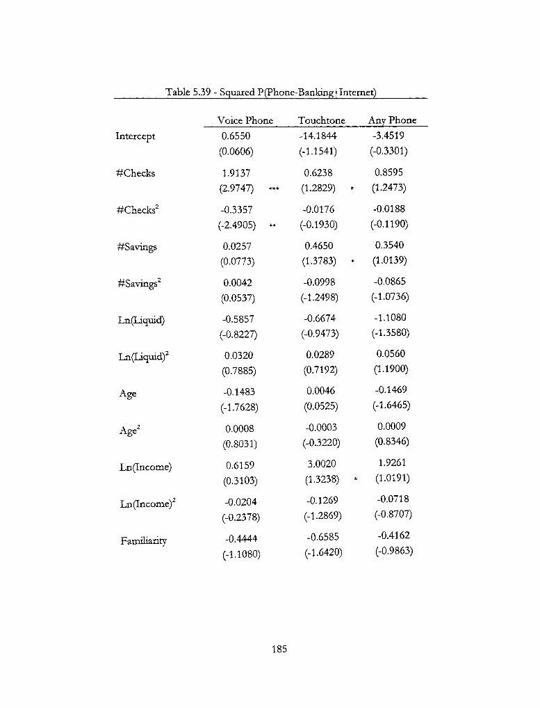
Table 5.39 - Squared P(Phone-Banking| Intemet)
Intercept
#Checks
#Checks'
#Savings
#Savings'
Ln(Liquid)
Ln(Liquid)'
Age
Age'
Ln(Income)
Ln (Income)"
FamiHarity
Voice Phone
0.6550
(0.0606)
1.9137
(2.9747) ***
-0.3357
(-2.4905) **
0.0257
(0.0773)
0.0042
(0.0537)
-0.5857
(-0.8227)
0.0320
(0.7885)
-0.1483
(-1.7628)
0.0008
(0.8031)
0.6159
(0.3103)
-0.0204
(-0.2378)
-0.4444
(-1.1080)
Touchtone
-14.1844
(-1.1541)
0.6238
(1.2829) *
-0.0176
(-0.1930)
0.4650
(1.3783) *
-0.0998
(-1.2498)
-0.6674
(-0.9473)
0.0289
(0.7192)
0.0046
(0.0525)
-0.0003
(-0.3220)
3.0020
(1.3238) *
-0.1269
(-1.2869)
-0.6585
(-1.6420)
Any Phone
-3.4519
(-0.3301)
0.8595
(1.2473)
-0.0188
(-0.1190)
0.3540
(1.0139)
-0.0865
(-1.0736)
-1.1080
(-1.3580)
0.0560
(1.1900)
-0.1469
(-1.6465)
0.0009
(0.8346)
1.9261
(1.0191)
-0.0718
(-0.8707)
-0.4162
(-0.9863)
185
Table 5.39 - continued
Risk* Age
Risk*NHS
Risk*HS
Risk*SC
Risk*BA
Risk*M7V
Risk*DR
Voice Phone
0.0175
(0.9916)
-0.5183
(-0.6380)
-0.5702
(-0.7555)
-0.7684
(-1.0309)
-0.7765
(-1.0409)
-0.1794
(-0.2319)
-1.0547
(-1.3135) *
Touchtone
0.0040
(0.2281)
-0.5701
(-0.6897)
-0.9095
(-1.1796)
-0.0693
(-0.0922)
-0.4012
(-0.5360)
-0.3152
(-0.4103)
-0.9462
(-1.1532)
Any Phone
0.0125
(0.6845)
-0.5861
(-0.6856)
-0.6934
(-0.8667)
-0.3218
(-0.4043)
-0.6528
(-0.8242)
-0.2605
(-0.3166)
-1.1361
(-1.3494) *
Note: ***, **," represent significance at the 99%, 95% and 90% levels, respectively
186
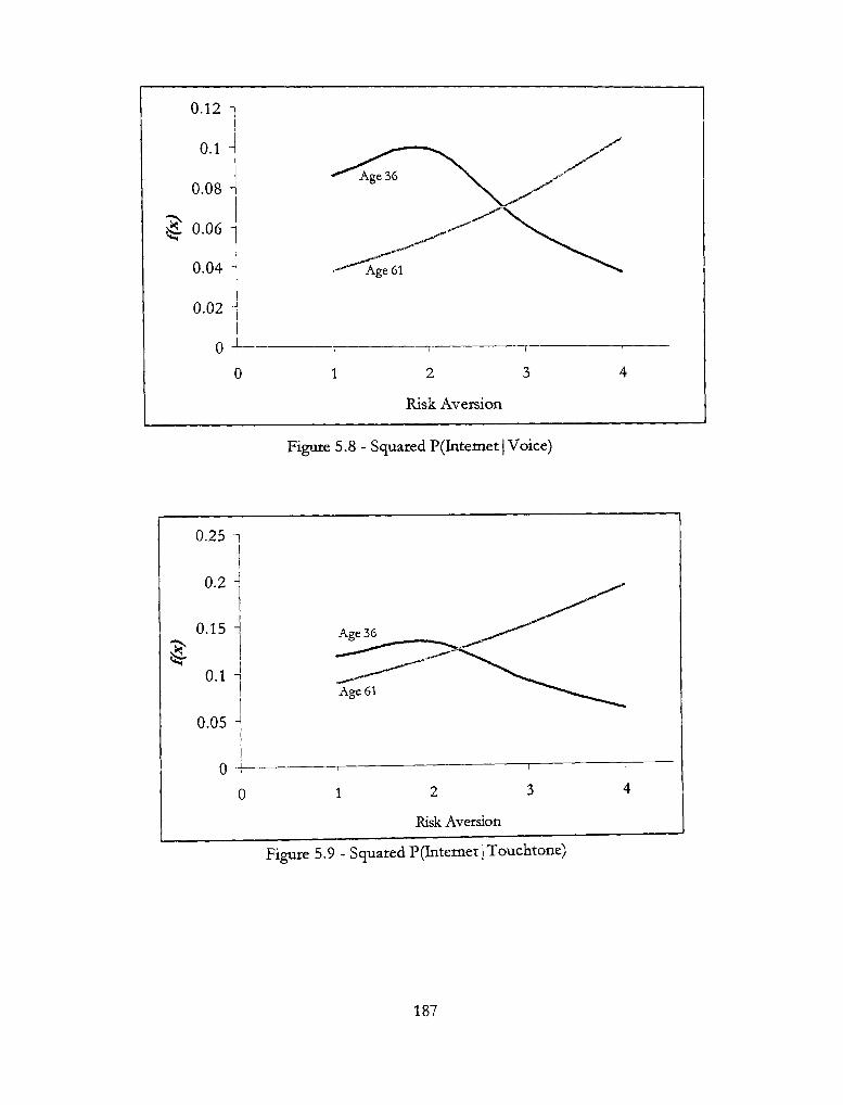
0.12 n
0.1 -
0.08 -
1^ 0.06 -
0.04 -
0.02 •
0
^ — ^
• " " j ^ g e 36 N.
•-"^g&fA
1 r
3 1 2
Risk Aversion
y
1
3 4
Figure 5.8 - Squared P(Intemet | Voice)
Figure 5.9 - Squared P(hitemet| Touchtone)
187
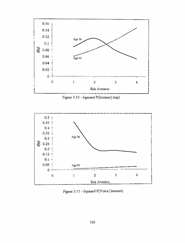
Figure 5.10 - Squared P(Intemet| Any)
0.5 1
0.45 -0.4 -
0.35 H 0.3 -
§ 0.25 -0.2 -1
0.15 -0.1 ^
0.05 -0 -
(
Age 36 \
Age 61
'
) 1
1
2 3
Risk Aversion
' 4
Figvure 5.11 - Squared P(Voice | Intemet)
188
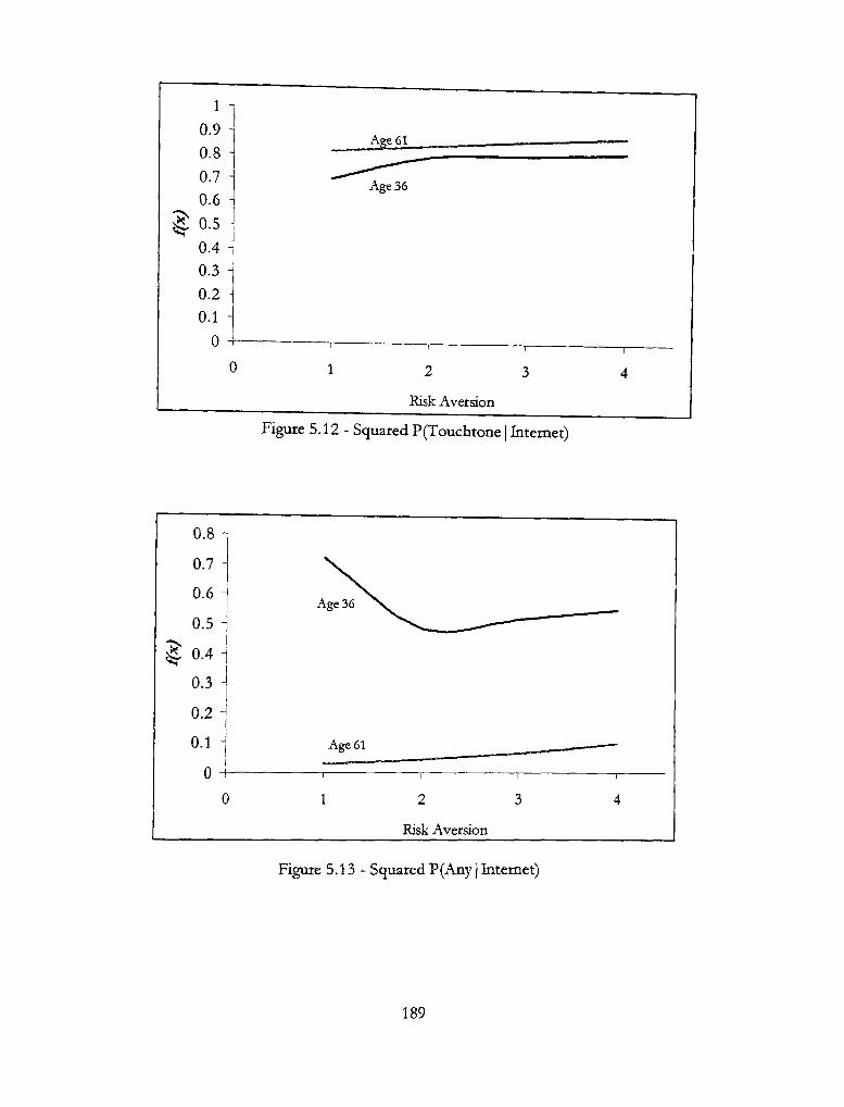
Figure 5.12 - Squared P(Touchtone | hitemet)
0.8 -
0.7 -
0.6 -
0.5 -]
^ 0.4-
0.3 -
0.2 -
0.1 -
0 -i
C
Age 36 N
Age 61 LU*J1
' ) 1
1 1
2 3
Risk Aversion
1
4
Figure 5.13 - Squared P(Any | Intemet)
189
CHAPTER 6
CONCLUSIONS AND CONTRIBUTIONS
The purpose of this chapter is to tie aU of the thesis together and explain the
contribution this research makes to the Hterature. The primary purpose of the conclusions
chapter is to puU aU chapters and sections of the paper together and summarize the
important findings. The contributions chapter wUl summarize how this research adds to our
knowledge of Internet banking from both an academic as weU as a practitioner's perspective.
6.1 Conclusions
This thesis began by introducing a problem in modem banking. Fast and growing
acceptance of the Intemet by individuals has prompted banks to invest heavUy in Intemet
banking infrastructure, hoping to reduce the cost of routine transactions. EventviaUy, many
bankers hope to be able to accept consumer loan appHcations via the Internet, credit score
the appHcation, and approve (or deny) the loan automaticaUy, even if the bank is closed.
These productivity gains can only be achieved if bank customers adopt Intemet banking.
Unfortunately, Intemet bankkig adoption has been slow. After weighting the
responses ki the 1998 SCF, it appears that only 4% of bank customers nationwide reported
using it, despite the fact that some 80% of smaU bank accounts woiUd have been offering the
service. The research question analyzed ki this thesis has been why Intemet bankkig has not
been adopted more readUy by banking customers.
To address this question, we presented a consumer choice model. We assumed that
bank customers faced with a choice of Internet versus conventional banking would choose
190
die configuration of bank access that would maxkkze expected consumer utUity. For
comparison purposes, we used conventional bankkig, Intemet bankkig and phone-bankkig
(a close substitute for Intemet bankkig). We showed tiiat rational utiHty maxknizkig bank
customers would accept aU remote access bankmg (or be mdifferent toward accepting tiiem)
if no risk were perceived. Subjective probabUity of adverse outcomes then becomes critical
ki assessing whether customers wUl choose to adopt Intemet banking or not.
When risk is present, adoption depends on added utiHty of the remote banking
service, added costs (a budget constrakit), and die size of the risk premium. The size of the
risk premium depends on die individuals risk aversion and the subjective probabihty
distribution that somethkig bad wiU happen. The added cost of remote banking wiU depend
on the type of remote banking (Intemet or phone-banking) and, in the case of Intemet
banking, on whether a computer and the training to mn it are sunk costs. Utihty gained
from remote banking could depend on many issues. We identified complexity of customers'
individual finances as one possibihty.
We showed that not only can Intemet banldng adoption be seen as a consumer
UtiHty maximization problem, but that the configuration of remote banking medium used by
the consumer can be seen as finding the marginal rate of substimrion that both equals the
budget constraint and has the highest utihty among the different configurations.
The knphcations of this theoretical analysis was that marginal utUity, marginal cost
and marginal risk premium were the only relevant variables to consider in determining
whether a consumer would adopt a new remote access method. Chapter 4 presented proxies
for the utihty, budget constraint and risk aversion components of our model, holding
subjective risk estimates constant (assuming homogeneity of subjective probabUity sets).
191
For kidividual remote access methods the model seemed to hold. The primary utUity
variable seems to be connected to the checking account, which suggests that in 1998
Intemet bankkig may have been seen primarily by customers as a way of managbg one's
checking account. The budget constraint appeared to be best modeled by kicome (a proxy
for whether a computer would have been pvurchased), age, education and famiHarity with
other Intemet financial services (proxying for the Hkehhood of having been trained in the
use of a computer and the Internet). The risk aversion responses to the SCF were used to
proxy customer risk aversion, and appeared to be strong predictors of Intemet adoption.
The phone-banking adoption decision tended to use more utiHty proxies, probably at
least partiaUy due to the larger number of reported users (larger sample size). In this case the
number of savings accounts and sometimes Hquid account balances were also good proxies
for UtUity. The same budget constraint variables seemed to be good predictors of phone-
bank usage, except other Internet financial services usage. And risk aversion was stiU an
important consideration, meaning that there was some risk perceived in accessing one's
account via any form of remote banking analyzed ki this thesis.
But the theoretical model imphed that utiHty would be maximized over aU remote
access banking options. Therefore a multinomial logit model was used to test if these
variables could be used to predict what configuration of remote bankkig options woiUd be
employed by bank customers. The overaU model explained a significant amount of the
variation and the predictor variables, for the most part, had die hypothesized signs. In aU
cases, risk aversion variables were knportant ki weighing die adoption deasion.
But die theory went further than just predicting tiiat tiie overaU configuration of
remote banking metiiods would depend on margkial utiHty, margkial cost and die size of die
192

marginal risk premium. These concepts would be important ki determining the marginal
decisions of adopting Intemet banking after phone-banking had been adopted, or vice versa.
This analysis is important because the a priori theory cannot predict the relative importance
of many of these variables. Those relating to computer and Intemet training should be
significant in marginal propensity to adopt Intemet banking, but the utUity and risk variables
are not predictable from the theory.
The test of tiiese hj^otheses showed that higher utiHty values led to higher
probabUity of marginal adoption propensity (going from phone-banking to Intemet or vice
versa). The computer related variables acted as expected. However, risk aversion was only
detected going from phone-banking to Intemet banking, there is no evidence of marginal
risk perceived by customers going from Internet banking to phone-banking. Since they are
distinct types of remote banking, and since risk aversion was an important factor with each
individual adoption decision, this finding is interesting. Risk is perceived moving from
conventional banking to phone-banking, but there is no evidence that customers perceive
any risk moving from Intemet banking to phone-banking. This not only imphes that in
general Intemet banking is perceived to be more risky, but that any and aU risks inherent in
phone bankkig are also kicluded ki Intemet bankkig, so diat movkig from Intemet bankkig
to phone banking creates no unique risks.
But this is not the only tkne where not findkig evidence piques our kiterest. Risk
aversion was found to be knportant ki determkikig whedier a customer would adopt die
Intemet. However, k was shown tiiat never was die Hquid account balance an knportant
predictor variable, not even when kiteracted witii tiie risk aversion variable. If one were
193
nervous about losing one's money, it is only logical that this variable would be negatively
related to adoption, but it was not. So another test was devised.
Correlation between the risk aversion response and the proportion of Hquid assets
held in the institution with Internet access was estknated, which was also not statisticaUy
significant. The interesting question this raises is if the risk aversion is so important to the
adoption decision, why is not the Hquid account balance variable sensitive to the risk
aversion for Internet banking adoption. One possible answer, which cannot be addressed
with this dataset, is that the customers may see the worst outcome as something worse than
an unauthorized withdrawal of Hquid assets. Since banks are information processor,
customers may be more worried about unauthorized access to financial information (i.e.,
identity theft), against which no deposit insvirance can protect. Whether this is the primary
concern is unclear from this research, but is an interesting foUow-up research question.
Simply showing that perceived risk is an important element in keeping customers
from adopting Intemet banking is not enough for banks to want to address it. The
subjective probabUity distribution must be shown to be maUeable. TheoreticaUy, the final
component in the consumer utihty optknization problem is tiie perceived risk premium.
This component has two parts, the risk aversion of tiie customer, and die subjective
probabUity distribution. If the subjective probabUity distribution differs among customers,
then variables affecting k could be kiteracted witii tiie risk aversion to better predict tiie risk
premium. We test this hypothesis by runnkig kiteractive variables, and find some
improvement ki die predictabUity of adoption. The variables proxykig for computer trakung
were tiiose which seemed to be die best for tiks kiteraction (botii education and age). This
194
suggests that svibjective probabihties are not uniform, meankig that banks should be able to
affect the risk premium.
In re-estimating the variables important in adopting Intemet banking given phone-
banking, some revisions needed to be made to our earher conclusions. Fkst, there may be
some perceived risk in moving from Intemet banking to voice phone-banking (the noted
doctoral risk premium). In addition, there may be some perceived theft risk detected in
Intemet bankkig for those customers akeady using touchtone banking.
But the tabular evidence presented in this research was not as surprising as the
graphical evidence. Analyzing the effect of risk aversion on the conditional probabUities of
adoption showed that perceived risk with Internet banking was primarily a drag on adoption
rates only for the youngest customers. For older customers, the Intemet either added no
noticeable risks or the risk premium was not the primary reason they did not adopt it.
In short, the slow adoption of Internet banking appears to the resvUt of rational
UtiHty maximization on the part of bank customers. To improve adoption rates, banks need
to offer services that truly improve utiHty to thek customers, cost them less and are easy to
access, and should present the customer with as Httie risk of adverse outcomes of any kind as
possible. As was pointed out earher, the most critical assumption in the model is that of
risk; if you can ehminate the risk, aU customers with the hardware and die trainkig would
adopt. Banks cannot affect customers' risk aversion, but they can affect die subjective
probabUity that somethkig bad wUl happen. The easiest way of affecting the subjective
probabUity seems to be tiirough trakkng. FmaUy, there appears to be a differing effect of
perceived risk depending on die age of the customer. Older customers probably need for
computer trainkig, whereas younger customers need to understand what risks reaUy exist.
195
; as an
6.2 Contributions
This research adds to die current academic Hterature ki several ways. Fkst, tiks
paper focuses on buskiesses diat offer bodi traditional and electronic channels and only
considers die factors knportant to consumers in chooskig to use electronic commerce :
additional not a substitute channel. The research to tiks pokit has focused on why
consumers would choose one channel over another, tiks research focuses on why consvimers
wovdd resist an additional channel if it could add more utUity.
Second, tiks paper tiieoreticaUy and empkicaUy analyzes the role of risk inherent in
the channel (the Intemet). As mentioned in the Hterature review chapter, aU other
researchers have focused on die concept of "trust." This concept had more to do with tmst
of the company than risk inherent in the Intemet as a secure method of transacting buskiess.
Since our model focuses on banks whose customers have akeady expressed thek tmst in the
firm, the relevant risks under study here refer to the medium through which that business is
conducted. As such, this is the only research that has been able to separate medium specific
risk from the concept of trust.
Thkd, this paper examines the role of perceived risk as it adds expected disutihty to
the current optimal bvindle. If bank customers can choose to use phone banldng, which
brings with it a certain amount of perceived risk, then the decision to adopt Intemet banking
is a decision that brings with it even more risk-risk that is unique to Intemet banking. This
risk brings with it a unique expected disutihty over and above the expected disutihty of using
phone banking.
196
Fourtii, this paper looks at the effect of non-uniform subjective probabUity
distributions on the Intemet bank adoption decision. Many academic financial economic
models assume homogeneity of subjective probabUity. This research assumes it eariy on to
test assumed outcomes of the model holdkig risk constant. However, once we aUow
perceived risk to vary among bank customers, the optknal model changes sHghtiy. It appears
that subjective probabUity sets are not identical across aU bank customers.
Fifth, and possibly least important, we have shown that in some instances, the
outcome of the test depends on the definition of phone-banking. In some instances, the
natvire of the phone-banking service either adds risk or requkes greater technical expertise.
As phone-banking is defined differentiy, variables become more or less important in
predicting adoption. If phone-banking is defined as either touchtone or voice access, some
precision is lost in the multinonkal model, and the interpretation of the conditional logits is
unclear.
6.2.1 Practical Contributions
In addition to the academic contributions, this paper adds to the practical
understanding of Internet bankkig. From a practical standpoint, banks wanting to kicrease
the adoption rate of Intemet banking should focus on three knportant concepts. Fkst, they
should buUd a system that adds utUity to the consumer. This simply means that the Intemet
bankkig services offered by the bank should solve a real problem faced by the consumer.
Second, die cost should be low. From our model, that means that fees should be as low as
possible (nothing for basic Intemet bankkig services), and tiie Intemet mterface should be as
user friendly as possible. The more user unfriendly the kiterface, the more computer Hterate
197
tiiek consvimers must be to use it, increasing the human capital cost for some. And finaUy,
although banks have no dkect influence on the consumer's risk aversion, they can affect the
risk premium (the last square bracket in Equation 3,6) by affectkig the subjective probabihty
distribution of security breaches.
Of the three areas banks can affect, reducing the risk premium is probably the most
important, since it was shown in Chapter 3 that as the subjective probabihty of security
breaches approaches zero (the model approaches the certainty model), aU consumers wUl
prefer the remote access account. For example, many credit cards address this opportunity
by "guaranteeing" that cvistomers wUl not have to pay for Intemet orders they did not place.
In many ways, this model is broadly consistent with what both Alba et al. (1997) and
Mols (1998) hypothesized about e-commerce; this model assumes that adoption is a function
of benefits versus the costs of adoption. However, there is a subtie difference in the
definition of the "trust" mechamsm. Prior papers have defkied tmst in terms of getting the
expected good or service. In this model the key to predicting remote banking adoption is
whether or not the expected utiHty is greater than the margkial cost. One of the key
components ki the expected utility is the perceived risks and outcomes of remote bankkig
technologies.
Although most bankers would not be svirprised to find that thek customers are
maxknizkig expected utiHties ki thek Intemet bankkig adoption decision, some of the detaUs
may be surpriskig. Many bankers would be surprised at die knportance of risk aversion ki
die decision, skice money deposited at kisured financial kistimtions is covered by deposk
insurance, makkig thek kivestments ki most bank accounts risk free.
198
As was pokited out earher there is not evidence that risk aversion has anythkig to do
with amount of money in Hquid accounts, and therefore there is no evidence that there is any
sensitivity on the part of risk averse bank customers to the money they would have "at risk"
by cyber-thieves.
In fact, much of the resistance to Intemet banking may in fact be hnked to this risk
aversion. A recent Wall Street Journal artide on Intemet banking suggested that the more
comphcated the transaction, the more likely the transaction would be conducted in a
traditional mamier, rather than on the Intemet (mortgages were used as an example)''. WTiat
bankers have interpreted as comphcated, customers may be interpreting as risky. Customers
may see a transaction as potentiaUy risky, because they may fear that if they miscommvimcate
information this wUl adversely affect the probabihty of getting a loan they sorely need. If
these tj^es of transactions are perceived as potentiaUy risky by consumers, then there is a
remedy; merely redesign the system to reduce the potential anxiety of bank customers. If the
process is hopelessly comphcated there may be no solution.
But risk aversion appears to only affect the decision making process of younger
consvimers. For older consumers, risk aversion has nothing to do with adoption. The best
explanation for this findkig is that die probabihty that somethkig adverse wUl occur given
remote bankkig adoption is perceived to be very high. The most hkely reason for this is that
older consumers have a high mistmst for computers. They are sure that tiiey can't use it.
To increase adoption among older consumers, banks could host Intemet and computer
training.
19 Rogers, Susannah. Keep on Smiling. Wall Street Journal, April 15, 2002, page RlO-Rll.
199
The final contribution foUows dkecdy from the last contribution. Although it may
not be possible to reduce the complexity of a mortgage loan appHcation, there is evidence
that perceived risk is somethkig that can be adjusted, given education or trakikig. If the
problem is not one of complexity, but of risk, there may be a solution.
6.2.2 Shortcomings and Future Research
Despite the findings of this paper, it has its drawbacks. Going back to the
theoretical chapter, we note that there were variables that we could not find in the dataset
For example, we hypothesized that cost of Internet banking would be relevant In the early
years of Intemet banldng, many banks charged fees for customers interested in Intemet
banking. This variable is not kicluded in the model presented in this paper, because it was
not provided in the SCF. In addition, tiiere may be many more appropriate variables
proxying for added utihty of Intemet banking. And the Hst could go on. The model could
be tested more fuUy and more appropriately with a more focused dataset, but such a dataset
was not available.
As in aU research, this thesis raised questions to be answered by later research. The
data set used, although the most recent at the tkne, is fakly early ki the adoption tknehne.
Whether things have changed over time is a good question we leave to others. Perhaps the
most pressing question left to others is what is k that bank customers fear. As pokited out
earher ki this chapter, we found no correktion between hquid assets avaUable electronicaUy
and nsk aversion. If bank customers are not sensitive to cyber-tikeves what is k tiiey fear?
From a practitioners' standpokit, tiks is tiie most knportant question left unanswered.
200
REFERENCES
Alba, J., Lynch, J., Weitz, B., Janiszewski, C , Lutz, R., Sawyer, A., et al. (1997). Interactive Home Shoppingr Consumer, RetaUer, and Manufacturer Incentives to Participate in Electroikc M'axk.etph.ces, Journal of Marketing, 61 Quly), 38-53.
Barth, J., Kraft, A., & Wiest, P. (1977). A UtUity Maxknization Approach to Individual Bank Asset Selection, Journal of Money, Credit and Banking, 9(2), 316-327.
Bakos, Y. & Brjrnjolfsson, E. (2000). Bundling and Competition on the Intemet, Marketing Science, 19(1), 63-82.
Benaroch, M., & Kauffman, R. (2000). Justifying Electronic Banking Network Expansion Using Real Options Analysis. MIS Quarterly, 24(2), 197-225.
Bielski, L. (2000, September). Online banking yet to dehver. ABA Banking Journal, pp. 6,12.
A big 'pop' for online banking. (2001, September). Bank Marketing, p. 8.
Bouckaert, J., & Degryse, H., (1995). Phonebanking. European Economic Review, 39 (2), 229-244.
Branch, SheUy (2002, February 11). Confessions of an Onhne Shopper. The Wall Street Journal, pp. R8, R16.
Brick and Block are Back. (2001, October). Bank Marketing, p. 8.
Brown, M., & Heien, D. (1972). The S-Branch Utihty Tree: A Generahzation of tiie linear Expenditure System. Econometrica, 40(4), 737-747.
Bruno, Mark (2001, October). Questions About Aggregation. USBanker, pp. 48-56.
Brynjofsson, E. & Smitii, M. (2000). Frictionless Commerce? A Comparison of Intemet and Conventional RetaUers. Management Science, 46(4), 563-585.
Bufinan, G., & Leiderman, L. (1993). Currency Substitution under Nonexpected Utihty: Some EmpinalEvidetice, Journal of Money, Credit and Banking, 25(3), 320-335.
Byers, R. & Lederer, P. (2001). RetaU Bank Services Strategy: A Model of Traditional, Electronic, and Mixed Distribution Chokes. Journal of Management Information Systems, 18(2), 133-156.
201
Calem, P. & Mester, L. (1995). Consumer Behavior and the Stickmess of Credit-Card Interest Rates. The American Economic Review, 85(5), 1327-1336.
Clemons, E., Hann, I., & Hitt, L. (1999). The Nature of Competition in Electronic Markets: An Empirical Investigation of Online Travel Agent Offerings. Unpubhshed Manuscript, University of Pennsylvania.
Cox, D. & JappeUi, T. (1993). The Effect of Borrowing Constrakits on Consumer LiabUities. Journal of Money, Credit and Banking, 2S(2), 197-213.
Crook, J. (2001). The Demand for Household Debt ki die USA: Evidence from die 1995 Survey of Consumer Fkiance. Applied Financial Economics, 11(1), 83-91,
Cvurtki, R., Juster, T., & Morgan, J. (1989). Svirvey Estknates of Wealth: An Assessment of Quahty. In R. lipsey and H. S. Tice (Eds), The Measurement of Savings Investment, and Wealth (pp. 473-548). Chicago: University of Chicago Press for NBER.
Daniel, D., Longbrake, W., & Murphy, N., (1973). The Effect of Technologj^ on Bank Econorrkes of Scale for Demand Deposits. Journal of Finance, 28(1), pp. 131-146.
Degeratu, A., Rangaswamy, A., & Wu, J. (2000). Consumer Choice Behavior in Online and Traditional Supermarkets: The Effects of Brand Name, Price, and other Search Attributes. Unpubhshed Manuscript, University of Pennsylvania.
Degryse, H., (1996). On the Interaction Between Vertical and Horizontal Product Differentiation: An AppHcation to Bankkig. The Journal of Industrial Economics, 44(2), 169-186.
Domowitz, I. (2001). IJquidity, Transaction Costs, and R^intermediation in Electronic Markets. Unpubhshed Manuscript, Penn State Universitj'.
Duca, J. & WhiteseU, W. (1995). Credit Cards and Money Demand: A Cross-sectional Study. Journal of Money, Credit and Banking, 21(^, 604-623.
Esser, J. (1999, October). Intemet Bankkig is a Vkmal Necessity. Credit Union Maga^ne, pp. 35-36.
Ewis, N., & Fisher, D. (1984). The Translog UtiHty Function and tiie Demand for Money ki the United St-ates, Journal of Money, Credit and Banking, 16(1), 34-52.
Furst, K., Lang, W., NoUe, D., (2000). Internet Banking. Development and Prospects. Economic and Policy Analysis, Unpubhshed Manuscript, Office of the ComptroUer of die Currency.
202
Gale, W. (1998). The Effects of Pensions on Household Wealtii: A Reevaluation of Theory and Evidence. The Journal of Political Economy, 106(4), 706-723.
Gale, W. & Scholz, J. (1994). IRAs and Household Savkig. The American Economic Review, 84(5), 1233-1260.
Goolsbee, A. (2000). In a Worid Witiiout Borders: The Impact of Taxes on Intemet Commexce. Quarterly Journal of Economics, 115(2), 561-576.
Hancock, D., Humphrey, D., & WUcox, J., (1999). Cost Reductions ki Electronic Payments: The Roles of ConsoHdation, Economies of Scale, and Technical Change. Journal of Banking & Finance, 23(2-4), ViXAlX.
Hannan, T., & McDoweU, J., (1984). The Detemikiants of Technologj^ Adoption: The Case of the Bankkig Fkm. Rand Journal of Economics, 15(3), 328-335.
Hannan, T., & McDoweU, J., (1987). Rival Precedence and the Dynamics of Technology Adoption: An Empirical Analysis. EwKOwzi , 54(214), 155-171.
Hannan, T., & McDoweU, J., (1990). The Impact of Technology Adoption on Market Structure. The Review of Economics and Statistics, 72(1), 164-168.
Heaton, J. & Lucas, D. (2000). Portfoho Choice and Asset Prices: The Importance of Entrepreneurial Risk. Journal of Finance, 55(3), 1163-1198.
Humphrey, D., & PuUey, L., (1997). Banks' Responses to Deregulation: Profits, Technology, and Efficiency. Journal of Money, Credit, andBanking, 29(1), 73-93.
Humphreys, K. (1999). Intemet Bankkig: Leadkig the Playkig Field for Community Banks, in J. Keyes (Ed.), Banking Technology Handbook (pp. 8-1 - 8-9). New York: CRC Press.
Hunter, W., & Tknee, S., (1986). Technical Change, Organizational Form and die Structure of Bank Production. Journal ofMong, Credit andBanking, 18(2), 152-166.
Hunter, W., & Tknme, S., (1991). Technological Change ki Large U.S. Commercial Banks, journal of Business, 64(3), 339-362.
Is Internet bankkig for you? (2001, March). Association Management, pp. 5-7.
IsraUevish, G. (2000). Review and Comments on Electronic Commerce Literature, Unpubhshed Manuscript, University of Chicago.
203
Jayawardhena, C. & Foley, P. (2000). Changes ki die Bankkig Sector - The Casee of Intemet Bankkig ki die U.K. Intemet Research: ElectronicNetworkingApplications andPolicy, 10(1), 19-
Jorgensen, D., & Lau, L. (1975). The Structure of Consumer Preferences, Annals of Economic and Social Measurement, 4(1), 49-101.
Juster, F., & Kuester, K. (1991). Differences ki die Measurement of Wealtii, Wealtii Inequaht}' and Wealdi Composition Obtakied From Alternative U.S. Wealdi Surveys. Review of Income and Wealth, 37(1), 33-62.
KennickeU, A. (1999). Revisions to the SCF Weighting Methodology: Accounting forRace/Ethnicity and Homeownership. Unpubhshed Manuscript, Federal Reserve Bank.
KennickeU, A., Starr-McClure, M., & Surette, B., (2000). Recent changes m U. S. famUy finances: results from the 1998 Survey of Consumer Fkiances. Board of Governors of the Federal Reserve System. Federal Reserve Bulletin. 86(1), p. 1-29.
KennickeU, A. & Woodbum R. (1999). Consistent Weight Design for die 1989, 1992, and 1995 SCFs and die Distribution of Wealtii. Remew of Income and Wealth, 45(2), 193-215.
Kingson, J. (2001, October 31). Home Bankkig Veteran: We've Come Far, But Nor Far Enough. American Banker, pp. 1,13.
Kmenta, J. (1987). Elements of Econometrics {X"^ ed.). New York: MacmUlan Pubhshing.
Lee, R. (2001, January 15). Keeping Freddie Krueger in the Closet: Intemet Security and OnHne Banking. Vital Speeches of the Day, pp. 210-213.
Lynch, J. & Ariely, D. (2000). Wine Online: Search Costs and Competition on Price, Quahty, and Distribution. Marketing Science, 19(1), 83-103.
MarHn, S. (2000, September). Study: 3,000 U.S. banks wUl offer e-bankkig services by 2005, Bank Systems (& Technologji, pp. 10.
Matutes, C. & PadUla A. (1994). Shared ATM Networks and Bankkig Competition. European Economic Review, 38(5), 1113-1138.
Mearian, L. (2001, September 3). Brick-and-chck bank sites outpackig online-only banks. Computerworld, pp. 12.
Mols, P. (1998). The Intemet and die Banks' Strategic Distribution Channel Decisions. Internet Research: Electronic Networking Applications andPolicy, 8(4), 331-337.
204

Mols, P. (2000). The Intemet and Services Marketing - The Case of Danish RetaU Bankkig. Intemet Research: Electronic Networking Applications andPolicy, 10(1), 7-18.
Moss, V. (2001, October). Aggregation is Comkig of Age. Credit Union Magat^ne, pp. 85-90.
MuUigan, C. (1999). Galton versus tiie Human Capital Approach to Inheritance. The Journal of Political Economy, 107(6), S184-S224.
Orr, B. (2001, July). Is Intemet Bankkig Profitable Yet? American Bankers Association. ABA Banking Journal, pp. 57-58.
Pratt, J. (1964). Risk Aversion in tiie SmaU and ki die Large, Econometrica, 32(1-2), 122-136.
Robkison, T. (2000, AprU 17). Intemet bankkig: StiU not a perfect marriage, Informationweek, pp. 104-106.
Rogers, S. (2002, AprU 15). Keep on SmUkig. The Wall Street Journal, pp. RlO-Rll.
Rose, M. (1999). Intemet Security Analysis Report: An Executive Overview. In J. Keyes (ed.). Banking Technology Handbook (pp. 32-1 - 32-7). New York: CRC Press.
Schacklett, M. (2000, January). Security Remakis a Major Issue for CUs and Thek Members. Credit Union Maga^ne, pp. 6-7.
Schwaiger, M. & Locarek-Jvmge, H. (1998, December). ReaHzkig Customer Retention Potentials by Electronic Banking [Electronic Version]. Electronic Markets, pp. 23-26.
Seungmook, C , & Kim, S. (1992). Structural Change in the Demand for Money, Journal of Money, Credit andBanking^ 24(2), 226-238.
Serietis, A., & Robb, A., (1986). Divisia Aggregation and Substitutabihty among Monetary Assets, Journal of Money, Credit and Banking, 18(4), 430-446.
Short, B., & ViUanueva, D. (1977). Further Evidence on the Role of Savkigs Deposits as Money in Canada. Journal of Money Banking and Credit, 9(3), 437-446.
Slywotzky, A. (2001, Summer). Revving the Engines of Onhne Fkiance. Mit Sloan Management Review, pp. 96.
Starr-McCluer, M. (1996). Health Insurance and Precautionary Savings. The American Economic Review, 86(1), 285-295.
Totty, M & Grimes A. (2002, Febmary 11). If at Fkst You Don't Succeed... The Wall Street Journal, pp. R6-R7.
205
Totty, P. (1999, July). On-line Security. Credit Union Magazine, pp. 70-71.
U.S. Department of Commerce. (1998). The EmergingDigitalEconomy (DHHS Pubhcation No. PB98-137029) [Electronic Version], Washkigton DC: U.S. Government Printing Office.
Urban, G., Sultan, F. & QuaUs, W. (1999). Design and Evaluation of a Trust Based Advisor on the Intemet. Unpubhshed Manuscript, Massachusetts Institute of Technology.
Wheelock, D., & WUson, P. (1999). Technical Progress, Inefficiency, and Productivity Change in U.S. Bankkig, \9%A'\99^, Journal of Money, Credit and Banking, 31(2), 212-234,
Wolff, E, (1992), Changkig Inequahty of Wealtii (ki Trends ki Nonwage Inequahty). The American Economic Remew, 82(2), 552-558.
206