percep- - carnegie mellon school of computer sciencerasc/download/amrobots5.pdfnavigation is one of...
TRANSCRIPT

5 Mobile Robot Localization 159
5 Mobile Robot Localization
5.1 Introduction
Navigation is one of the most challenging competencies required of a mobile robot. Successin navigation requires success at the four building blocks of navigation (fig. 5.2): percep-tion- the robot must interpret its sensors to extract meaningful data; localization- the robotmust determine its position in the environment; cognition- the robot must decide how to actto achieve its goals; and motion control- the robot must modulate its motor outputs toachieve the desired trajectory.
Of these four components, localization has received the greatest research attention in thepast decade and, as a result, significant advances have been made on this front. In this chap-ter, we will explore the successful localization methodologies of recent years. First, Section5.2 describes how sensor and effector uncertainty is responsible for the difficulties of local-ization. Then, Section 5.3 describes two extreme approaches to dealing with the challengeof robot localization: avoiding localization altogether, and performing explicit map-basedlocalization. The remainder of the chapter discusses the question of representation, then pre-sents case studies of successful localization systems using a variety of representations andtechniques to achieve mobile robot localization competence.
Fig 5.1 Where am I?
?
R. Siegwart, EPFL, Illah Nourbakhsh, CMU

160 Autonomous Mobile Robots
Observation
Mapdata base
Prediction ofPosition
(e.g. odometry)
Fig 5.2 General schematic for mobile robot localization.
Per
cept
ion
Matching
Position Update(Estimation?)
raw sensor data orextracted features
predicted position
position
matchedobservations
YES
Encoder

5 Mobile Robot Localization 161
5.2 The Challenge of Localization: noise and aliasing
If one could attach an accurate GPS (Global Position System) sensor to a mobile robot, muchof the localization problem would be obviated. The GPS would inform the robot of its exactposition and orientation, indoors and outdoors, so that the answer to the question, "Wheream I?" would always be immediately available. Unfortunately, such a sensor is not currentlypractical. The existing GPS network provides accuracy to within several meters, which isunacceptable for localizing human-scale mobile robots as well as miniature mobile robotssuch as desk robots and the body-navigating nano-robots of the future. Furthermore, GPStechnologies cannot function indoors or in obstructed areas and are thus limited in theirworkspace.
But, looking beyond the limitations of GPS, localization implies more than knowing one’sabsolute position in the Earth’s reference frame. Consider a robot that is interacting with hu-mans. This robot may need to identify its absolute position, but its relative position with re-spect to target humans is equally important. Its localization task can include identifyinghumans using its sensor array, then computing its relative position to the humans. Further-more, during the Cognition step a robot will select a strategy for achieving its goals. If it in-tends to reach a particular location, then localization may not be enough. The robot mayneed to acquire or build an environmental model, a map, that aids it in planning a path to thegoal. Once again, localization means more than simply determining an absolute pose inspace; it means building a map, then identifying the robot’s position relative to that map.
Clearly, the robot’s sensors and effectors play an integral role in all the above forms of lo-calization. It is because of the inaccuracy and incompleteness of these sensors and effectorsthat localization poses difficult challenges. This section identifies important aspects of thissensor and effector suboptimality.
5.2.1 Sensor Noise
Sensors are the fundamental robot input for the process of perception, and therefore the de-gree to which sensors can discriminate world state is critical. Sensor noise induces a limi-tation on the consistency of sensor readings in the same environmental state and, therefore,on the number of useful bits available from each sensor reading. Often, the source of sensornoise problems is that some environmental features are not captured by the robot’s represen-tation and are thus overlooked.
For example, a vision system used for indoor navigation in an office building may use thecolor values detected by its color CCD camera. When the sun is hidden by clouds, the illu-mination of the building’s interior changes due to windows throughout the building. As aresult, hue values are not constant. The color CCD appears noisy from the robot’s perspec-tive as if subject to random error, and the hue values obtained from the CCD camera will beunusable, unless the robot is able to note the position of the Sun and clouds in its represen-tation.
Illumination dependency is only one example of the apparent noise in a vision-based sensorsystem. Picture jitter, signal gain, blooming and blurring are all additional sources of noise,potentially reducing the useful content of a color video image.
R. Siegwart, EPFL, Illah Nourbakhsh, CMU
162 Autonomous Mobile Robots
Consider the noise level (i.e. apparent random error) of ultrasonic range-measuring sensors(e.g. sonars) as we discussed in Section 4.1.2.3. When a sonar transducer emits sound to-wards a relatively smooth and angled surface, much of the signal will coherently reflectaway, failing to generate a return echo. Depending on the material characteristics, a smallamount of energy may return nonetheless. When this level is close to the gain threshold ofthe sonar sensor, then the sonar will, at times, succeed and, at other times, fail to detect theobject. From the robot’s perspective, a virtually unchanged environmental state will resultin two different possible sonar readings: one short, and one long.
The poor signal to noise ratio of a sonar sensor is further confounded by interference be-tween multiple sonar emitters. Often, research robots have between 12 to 48 sonars on a sin-gle platform. In acoustically reflective environments, multipath interference is possiblebetween the sonar emissions of one tranducer and the echo detection circuitry of anothertransducer. The result can be dramatically large errors (i.e. underestimation) in ranging val-ues due to a set of coincidental angles. Such errors occur rarely, less than 1% of the time,and are virtually random from the robot’s perspective.
In conclusion, sensor noise reduces the useful information content of sensor readings. Clear-ly, the solution is to take multiple readings into account, employing temporal fusion ormulti-sensor fusion to increase the overall information content of the robot’s inputs.
5.2.2 Sensor Aliasing
A second shortcoming of mobile robot sensors causes them to yield little information con-tent, further exacerbating the problem of perception and, thus, localization. The problem,known as sensor aliasing, is a phenomenon that humans rarely encounter. The human sen-sory system, particularly the visual system, tends to receive unique inputs in each unique lo-cal state. In other words, every different place looks different. The power of this uniquemapping is only apparent when one considers situations where this fails to hold. Considermoving through an unfamiliar building that is completely dark. When the visual system seesonly black, one’s localization system quickly degrades. Another useful example is that of ahuman-sized maze made from tall hedges. Such mazes have been created for centuries, andhumans find them extremely difficult to solve without landmarks or clues because, withoutvisual uniqueness, human localization competence degrades rapidly.
In robots, the non-uniqueness of sensors readings, or sensor aliasing, is the norm and not theexception. Consider a narrow-beam rangefinder such as ultrasonic or infrared rangefinders.This sensor provides range information in a single direction without any additional data re-garding material composition such as color, texture and hardness. Even for a robot with sev-eral such sensors in an array, there are a variety of environmental states that would triggerthe same sensor values across the array. Formally, there is a many-to-one mapping from en-vironmental states to the robot’s perceptual inputs. Thus, the robot’s percepts cannot distin-guish from among these many states. A classical problem with sonar-based robots involvesdistinguishing between humans and inanimate objects in an indoor setting. When facing anapparent obstacle in front of itself, should the robot say "Excuse me" because the obstaclemay be a moving human, or should the robot plan a path around the object because it maybe a cardboard box? With sonar alone, these states are aliased and differentiation is impos-

5 Mobile Robot Localization 163
sible.
The problem posed to navigation because of sensor aliasing is that, even with noise-free sen-sors, the amount of information is generally insufficient to identify the robot’s position froma single percept reading. Thus techniques must be employed by the robot programmer thatbase the robot’s localization on a series of readings and, thus, sufficient information to re-cover the robot’s position over time.
5.2.3 Effector Noise
The challenges of localization do not lie with sensor technologies alone. Just as robot sen-sors are noisy, limiting the information content of the signal, so robot effectors are alsonoisy. In particular, a single action taken by a mobile robot may have several different pos-sible results, even though from the robot’s point of view the initial state before the actionwas taken is well-known.
In short, mobile robot effectors introduce uncertainty about future state. Therefore the sim-ple act of moving tends to increase the uncertainty of a mobile robot. There are, of course,exceptions. Using cognition, the motion can be carefully planned so as to minimize this ef-fect, and indeed sometimes to actually result in more certainty. Furthermore, when the robotactions are taken in concert with careful interpretation of sensory feedback, it can compen-sate for the uncertainty introduced by noisy actions using the information provided by thesensors.
First, however, it is important to understand the precise nature of the effector noise that im-pacts mobile robots. It is important to note that, from the robot’s point of view, this error inmotion is viewed as error in odometry, or the robot’s inability to estimate its own positionover time using knowledge of its kinematics and dynamics. The true source of error gener-ally lies in an incomplete model of the environment. For instance, the robot does not modelthe fact that the floor may be sloped, the wheels may slip, and a human may push the robot.All of these un-modeled sources of error result in inaccuracy between the physical motionof the robot, the intended motion of the robot and the proprioceptive sensor estimates of mo-tion.
In odometry (wheel sensors only) and dead reckoning (also heading sensors) the position up-date is based on proprioceptive sensors. The movement of the robot, sensed with wheel en-coders and /or heading sensors is integrated to compute position. Because the sensormeasurement errors are integrated, the position error accumulates over time. Thus the posi-tion has to be updated from time to time by other localization mechanisms. Otherwise therobot is not able to maintain a meaningful position estimate in long run.
In the following we will concentrate on odometry based on the wheel sensor readings of adifferential drive robot only (see also [3, 40, 41]). Using additional heading sensors (e.g. gy-roscope) can help to reduce the cumulative errors, but the main problems remain the same.
There are many sources of odometric error, from environmental factors to resolution:
• Limited resolution during integration (time increments, measurement resolution,etc.)
• Misalignment of the wheels (deterministic)
R. Siegwart, EPFL, Illah Nourbakhsh, CMU

164 Autonomous Mobile Robots
• Unequal wheel diameter (deterministic)
• Variation in the contact point of the wheel
• Unequal floor contact (slipping, non-planar surface, etc.)
Some of the errors might be deterministic (systematic), thus they can be eliminated by prop-er calibration of the system. However, there are still a number of non-deterministic (ran-dom) errors which remain, leading to uncertainties in position estimation over time. From ageometric point of view one can classify the errors into three types:
• Range error: integrated path length (distance) of the robots movement-> sum of the wheel movements
• Turn error: similar to range error, but for turns-> difference of the wheel motions
• Drift error: difference in the error of the wheels leads to an error in the robot’s angularorientation
Over long periods of time, turn and drift errors far outweigh range errors, since their con-tribute to the overall position error is nonlinear. Consider a robot, whose position is initiallyperfectly well-known, moving forward in a straight line along the x axis. The error in the y-
position introduced by a move of d meters will have a component of , which can be
quite large as the angular error ∆θ grows. Over time, as a mobile robot moves about the en-vironment, the rotational error between its internal reference frame and its original referenceframe grows quickly. As the robot moves away from the origin of these reference frames,the resulting linear error in position grows quite large. It is instructive to establish an errormodel for odometric accuracy and see how the errors propagate over time.
5.2.4 An Error Model for Odometric Position Estimation
Generally the pose (position) of a robot is represented by the vector
. (5.1)
For a differential drive robot the position can be estimated starting from a known position
d ∆θsin
Fig 5.3 Movement of a differential drive robot
v(t)
ω(t)
θ
yI
xI
px
y
θ
=
5 Mobile Robot Localization 165
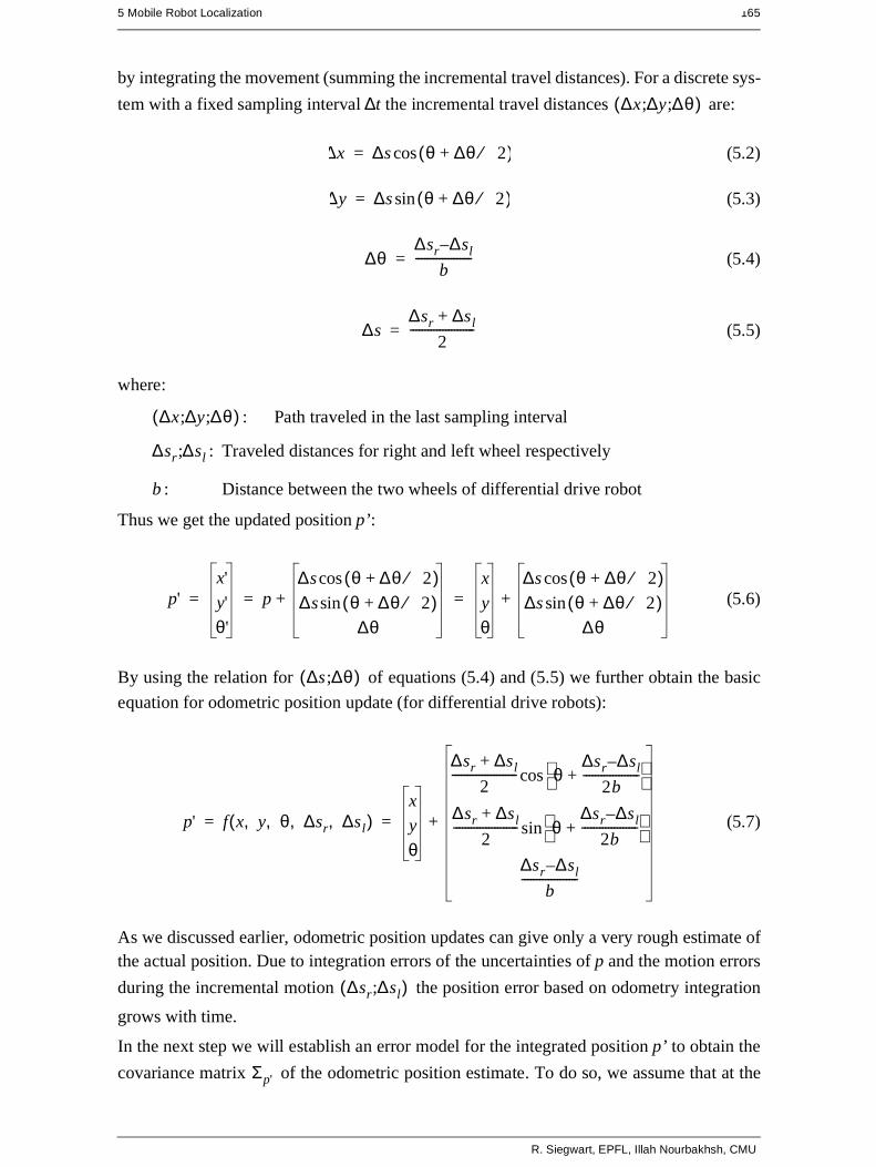
by integrating the movement (summing the incremental travel distances). For a discrete sys-
tem with a fixed sampling interval ∆t the incremental travel distances are:
(5.2)
(5.3)
(5.4)
(5.5)
where:
: Path traveled in the last sampling interval
: Traveled distances for right and left wheel respectively
: Distance between the two wheels of differential drive robot
Thus we get the updated position p’:
(5.6)
By using the relation for of equations (5.4) and (5.5) we further obtain the basic
equation for odometric position update (for differential drive robots):
(5.7)
As we discussed earlier, odometric position updates can give only a very rough estimate ofthe actual position. Due to integration errors of the uncertainties of p and the motion errors
during the incremental motion the position error based on odometry integration
grows with time.
In the next step we will establish an error model for the integrated position p’ to obtain the
covariance matrix of the odometric position estimate. To do so, we assume that at the
∆x ∆y ∆θ;;( )
∆x ∆s θ ∆θ 2⁄+( )cos=
∆y ∆s θ ∆θ 2⁄+( )sin=
∆θ∆sr ∆– sl
b-------------------=
∆s∆sr ∆sl+
2----------------------=
∆x ∆y ∆θ;;( )
∆sr ∆sl;
b
p'x'
y'
θ'p∆s θ ∆θ 2⁄+( )cos
∆s θ ∆θ 2⁄+( )sin
∆θ
+x
y
θ
∆s θ ∆θ 2⁄+( )cos
∆s θ ∆θ 2⁄+( )sin
∆θ
+= = =
∆s ∆θ;( )
p' f x y θ ∆sr ∆sl, , , ,( )x
y
θ
∆sr ∆sl+
2---------------------- θ
∆sr ∆– sl
2b-------------------+
cos
∆sr ∆sl+
2---------------------- θ
∆sr ∆– sl
2b-------------------+
sin
∆sr ∆– sl
b-------------------
+= =
∆sr ∆sl;( )
Σp'
R. Siegwart, EPFL, Illah Nourbakhsh, CMU
166 Autonomous Mobile Robots
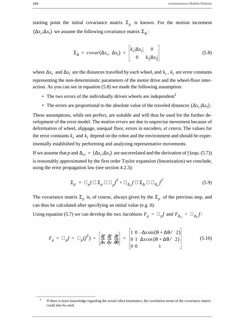
starting point the initial covariance matrix is known. For the motion increment
we assume the following covariance matrix :
(5.8)
where and are the distances travelled by each wheel, and , are error constants
representing the non-deterministic parameters of the motor drive and the wheel-floor inter-action. As you can see in equation (5.8) we made the following assumption:
• The two errors of the individually driven wheels are independent1
• The errors are proportional to the absolute value of the traveled distances .
These assumptions, while not perfect, are suitable and will thus be used for the further de-velopment of the error model. The motion errors are due to unprecise movement because ofdeformation of wheel, slippage, unequal floor, errors in encoders, et cetera. The values for
the error constants and depend on the robot and the environment and should be exper-
imentally established by performing and analyzing representative movements.
If we assume that p and are uncorrelated and the derivation of f (equ. (5.7))
is reasonably approximated by the first order Taylor expansion (linearization) we conclude,using the error propagation law (see section 4.2.3):
(5.9)
The covariance matrix is, of course, always given by the of the previous step, and
can thus be calculated after specifying an initial value (e.g. 0).
Using equation (5.7) we can develop the two Jacobians and :
(5.10)
1. If there is more knowledge regarding the actual robot kinematics, the correlation terms of the covariance matrixcould also be used.
Σp
∆sr ∆sl;( ) Σ∆
Σ∆ covar ∆sr ∆sl,( )kr ∆sr 0
0 kl ∆sl
= =
∆sr ∆sl kr kl
∆sr ∆sl;( )
kr kl
∆rl ∆sr ∆sl;( )=
Σp' ∇ pf Σp ∇⋅pfT⋅ ∇ ∆rl
f Σ∆ ∇ ∆rlf⋅ T⋅+=
Σp Σp'
Fp ∇ pf= F∆rl∇ ∆rl
f=
Fp ∇ pf ∇ p fT( ) f∂
x∂----- f∂
y∂----- f∂θ∂
------1 0 ∆s θ ∆θ 2⁄+( )sin–
0 1 ∆s θ ∆θ 2⁄+( )cos
0 0 1
= = = =
5 Mobile Robot Localization 167
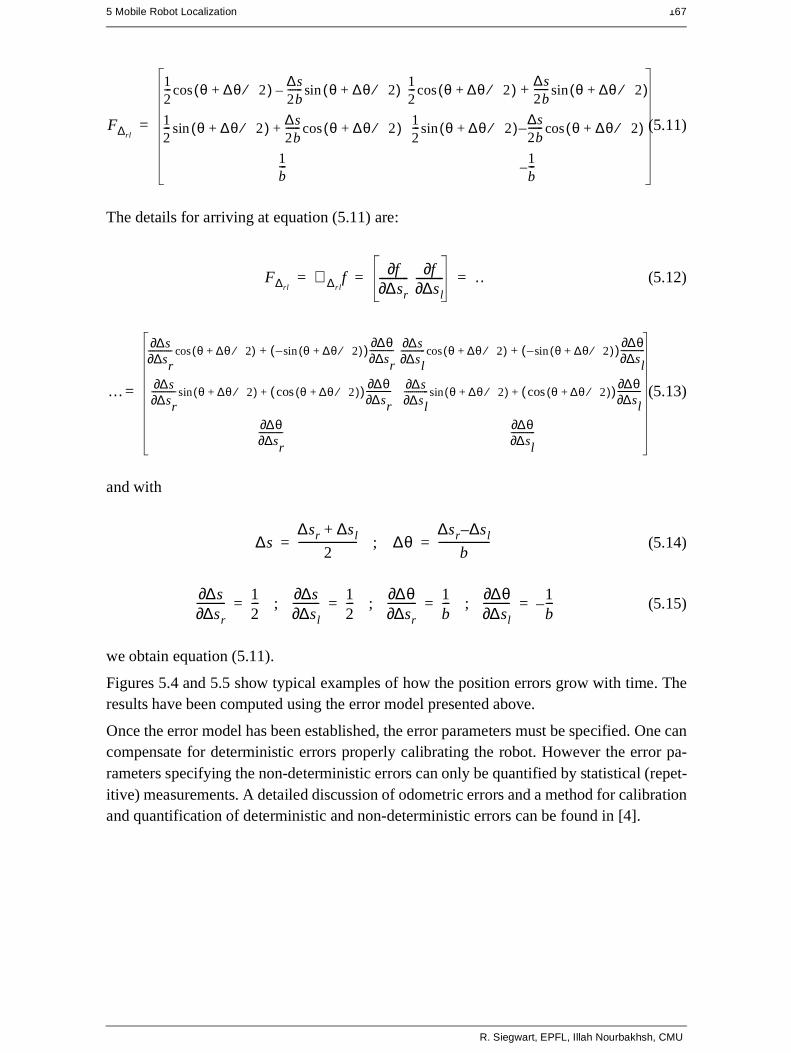
(5.11)
The details for arriving at equation (5.11) are:
(5.12)
(5.13)
and with
; (5.14)
; ; ; (5.15)
we obtain equation (5.11).
Figures 5.4 and 5.5 show typical examples of how the position errors grow with time. Theresults have been computed using the error model presented above.
Once the error model has been established, the error parameters must be specified. One cancompensate for deterministic errors properly calibrating the robot. However the error pa-rameters specifying the non-deterministic errors can only be quantified by statistical (repet-itive) measurements. A detailed discussion of odometric errors and a method for calibrationand quantification of deterministic and non-deterministic errors can be found in [4].
F∆rl
12--- θ ∆θ 2⁄+( ) ∆s
2b------ θ ∆θ 2⁄+( )sin–cos
12--- θ ∆θ 2⁄+( ) ∆s
2b------ θ ∆θ 2⁄+( )sin+cos
12--- θ ∆θ 2⁄+( ) ∆s
2b------ θ ∆θ 2⁄+( )cos+sin
12--- θ ∆θ 2⁄+( ) ∆s
2b------– θ ∆θ 2⁄+( )cossin
1b--- 1
b---–
=
F∆rl∇ ∆rl
f f∂∆sr∂
----------- f∂∆sl∂
---------- …= = =
…
∆s∂∆sr∂
------------ θ ∆θ 2⁄+( ) θ ∆θ 2⁄+( )sin–( ) ∆θ∂∆sr∂------------+cos
∆s∂∆sl∂
------------ θ ∆θ 2⁄+( ) θ ∆θ 2⁄+( )sin–( ) ∆θ∂∆sl∂------------+cos
∆s∂∆sr∂
------------ θ ∆θ 2⁄+( ) θ ∆θ 2⁄+( )cos( ) ∆θ∂∆sr∂------------+sin
∆s∂∆sl∂
------------ θ ∆θ 2⁄+( ) θ ∆θ 2⁄+( )cos( ) ∆θ∂∆sl∂------------+sin
∆θ∂∆sr∂
------------ ∆θ∂∆sl∂
------------
=
∆s∆sr ∆sl+
2----------------------= ∆θ
∆sr ∆– sl
b-------------------=
∆s∂∆sr∂
----------- 12---=
∆s∂∆sl∂
---------- 12---=
∆θ∂∆sr∂
----------- 1b---=
∆θ∂∆sl∂
---------- 1b---–=
R. Siegwart, EPFL, Illah Nourbakhsh, CMU

168 Autonomous Mobile Robots
Fig 5.4 Growth of the pose uncertainty for straight line movement: Note that the un-certainty in y grows much faster than in the direction of movement. This re-sults from the integration of the uncertainty about the robot’s orientation.The ellipses drawn around the robot positions represent the uncertainties inthe x,y direction (e.g. ). The uncertainty of the orientation is not rep-resented in the picture although its effect can be indirectly observed.
3σ θ
0 0.5 1
-0.4
-0.2
0
0.2
0.4
Error Propagation in Odometry
x [m]
y [m
]
Fig 5.5 Growth of the pose uncertainty for circular movement (r=const): Again, theuncertainty perpendicular to the movement grows much faster than that inthe direction of movement. Note that the main axis of the uncertainty ellipsisdoes not remain perpendicular to the direction of movement.
0 0.2 0.4 0.6 0.8 10
0.1
0.2
0.3
0.4
0.5
0.6
0.7
0.8
0.9
Error Propagation in Odometry
x [m]
y [m
]

5 Mobile Robot Localization 169
5.3 To Localize or Not to Localize: localization-based nav-
igation versus programmed solutions
Figure 5.6 depicts a standard indoor environment that a mobile robot navigates. Supposethat the mobile robot in question must deliver messages between two specific rooms in thisenvironment: rooms A and B. In creating a navigation system, it is clear that the mobile ro-bot will need sensors and a motion control system. Sensors are absolutely required to avoidhitting moving obstacles such as humans, and some motion control system is required so thatthe robot can deliberately move.
It is less evident, however, whether or not this mobile robot will require a localization sys-tem. Localization may seem mandatory in order to successfully navigate between the tworooms. It is through localizing on a map, after all, that the robot can hope to recover its po-sition and detect when it has arrived at the goal location. It is true that, at the least, the robotmust have a way of detecting the goal location. However, explicit localization with refer-ence to a map is not the only strategy that qualifies as a goal detector.
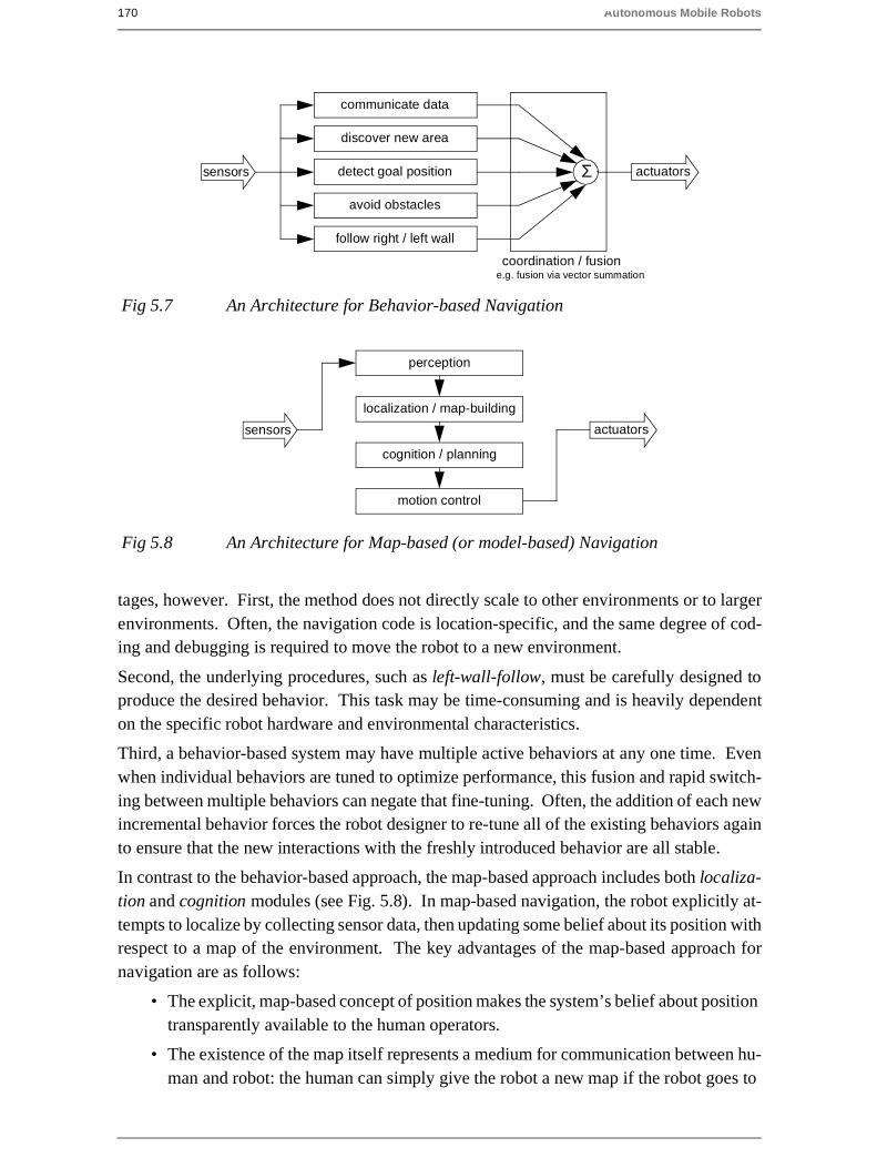
An alternative, espoused by the behavior-based community, suggests that, since sensors andeffectors are noisy and information-limited, one should avoid creating a geometric map forlocalization. Instead, this community suggests designing sets of behaviors that together re-sult in the desired robot motion. Fundamentally, this approach avoids explicit reasoningabout localization and position, and thus generally avoids explicit path planning as well.
This technique is based on a belief that there exists a procedural solution to the particularnavigation problem at hand. For example, in Fig. 5.6, the behavioralist approach to navigat-ing from Room A to Room B might be to design a left-wall-following behavior and a detec-tor for Room B that is triggered by some unique queue in Room B, such as the color of thecarpet. Then, the robot can reach Room B by engaging the left wall follower with the RoomB detector as the termination condition for the program.
The architecture of this solution to a specific navigation problem is shown in figure 5.7. Thekey advantage of this method is that, when possible, it may be implemented very quickly fora single environment with a small number of goal positions. It suffers from some disadvan-
Fig 5.6 A Sample Environment
A
B
R. Siegwart, EPFL, Illah Nourbakhsh, CMU
170 Autonomous Mobile Robots
tages, however. First, the method does not directly scale to other environments or to largerenvironments. Often, the navigation code is location-specific, and the same degree of cod-ing and debugging is required to move the robot to a new environment.
Second, the underlying procedures, such as left-wall-follow, must be carefully designed toproduce the desired behavior. This task may be time-consuming and is heavily dependenton the specific robot hardware and environmental characteristics.
Third, a behavior-based system may have multiple active behaviors at any one time. Evenwhen individual behaviors are tuned to optimize performance, this fusion and rapid switch-ing between multiple behaviors can negate that fine-tuning. Often, the addition of each newincremental behavior forces the robot designer to re-tune all of the existing behaviors againto ensure that the new interactions with the freshly introduced behavior are all stable.
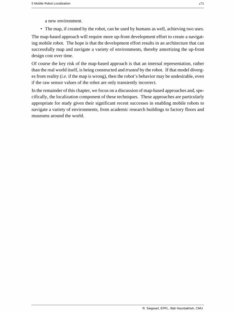
In contrast to the behavior-based approach, the map-based approach includes both localiza-tion and cognition modules (see Fig. 5.8). In map-based navigation, the robot explicitly at-tempts to localize by collecting sensor data, then updating some belief about its position withrespect to a map of the environment. The key advantages of the map-based approach fornavigation are as follows:
• The explicit, map-based concept of position makes the system’s belief about positiontransparently available to the human operators.
• The existence of the map itself represents a medium for communication between hu-man and robot: the human can simply give the robot a new map if the robot goes to
Fig 5.7 An Architecture for Behavior-based Navigation
sensors detect goal position
discover new area
avoid obstacles
follow right / left wall
communicate data
actuators
coordination / fusione.g. fusion via vector summation
Σ
Fig 5.8 An Architecture for Map-based (or model-based) Navigation
sensors
cognition / planning
localization / map-building
motion control
perception
actuators
5 Mobile Robot Localization 171
a new environment.
• The map, if created by the robot, can be used by humans as well, achieving two uses.
The map-based approach will require more up-front development effort to create a navigat-ing mobile robot. The hope is that the development effort results in an architecture that cansuccessfully map and navigate a variety of environments, thereby amortizing the up-frontdesign cost over time.
Of course the key risk of the map-based approach is that an internal representation, ratherthan the real world itself, is being constructed and trusted by the robot. If that model diverg-es from reality (i.e. if the map is wrong), then the robot’s behavior may be undesirable, evenif the raw sensor values of the robot are only transiently incorrect.
In the remainder of this chapter, we focus on a discussion of map-based approaches and, spe-cifically, the localization component of these techniques. These approaches are particularlyappropriate for study given their significant recent successes in enabling mobile robots tonavigate a variety of environments, from academic research buildings to factory floors andmuseums around the world.
R. Siegwart, EPFL, Illah Nourbakhsh, CMU
172 Autonomous Mobile Robots
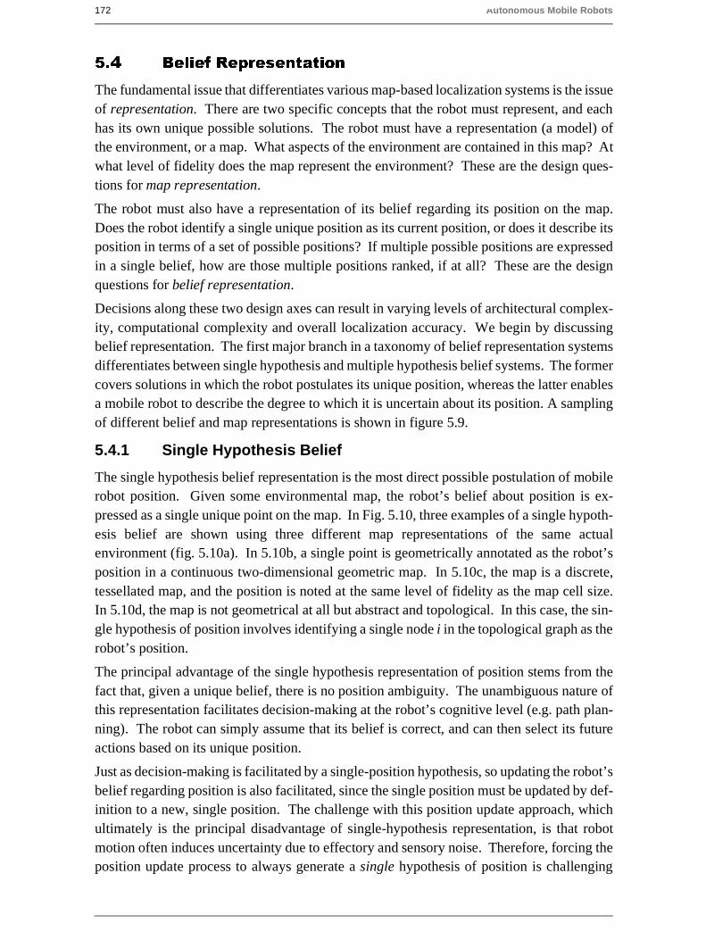
5.4 Belief Representation
The fundamental issue that differentiates various map-based localization systems is the issueof representation. There are two specific concepts that the robot must represent, and eachhas its own unique possible solutions. The robot must have a representation (a model) ofthe environment, or a map. What aspects of the environment are contained in this map? Atwhat level of fidelity does the map represent the environment? These are the design ques-tions for map representation.
The robot must also have a representation of its belief regarding its position on the map.Does the robot identify a single unique position as its current position, or does it describe itsposition in terms of a set of possible positions? If multiple possible positions are expressedin a single belief, how are those multiple positions ranked, if at all? These are the designquestions for belief representation.
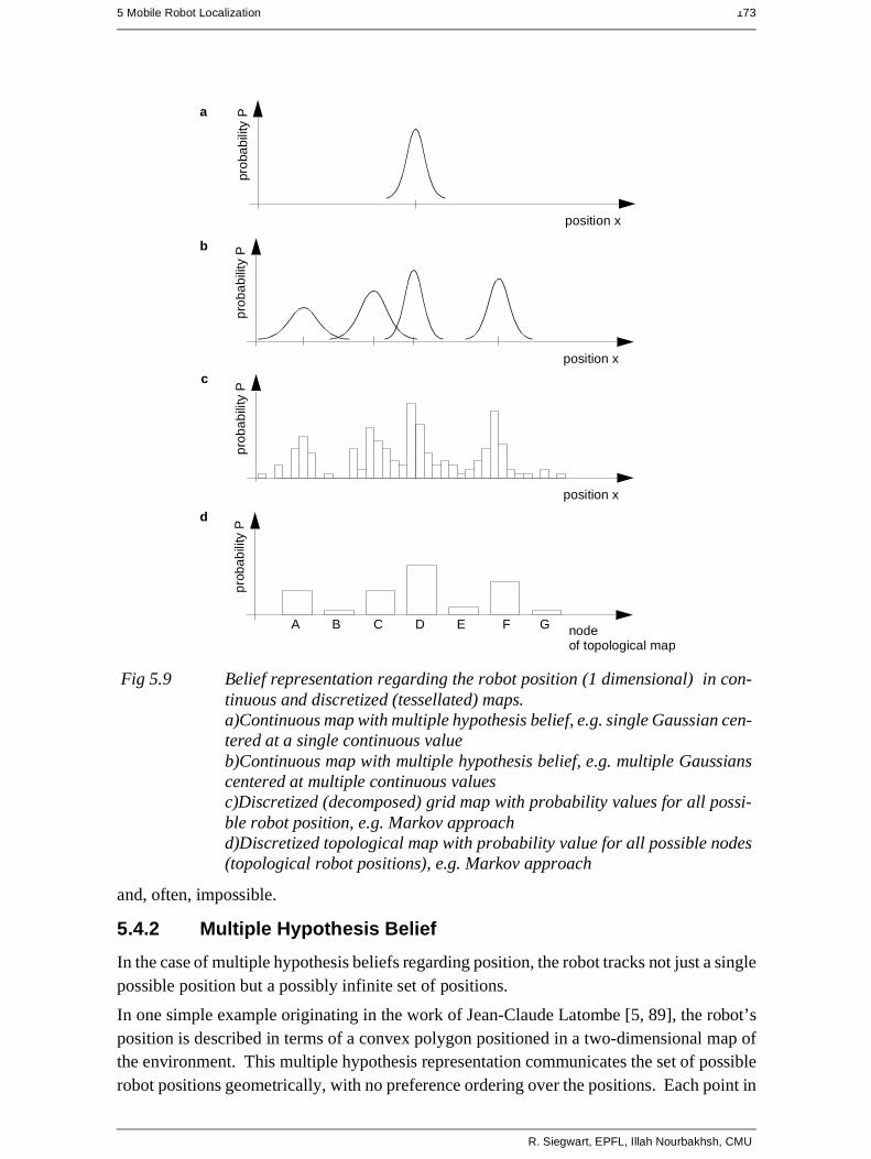
Decisions along these two design axes can result in varying levels of architectural complex-ity, computational complexity and overall localization accuracy. We begin by discussingbelief representation. The first major branch in a taxonomy of belief representation systemsdifferentiates between single hypothesis and multiple hypothesis belief systems. The formercovers solutions in which the robot postulates its unique position, whereas the latter enablesa mobile robot to describe the degree to which it is uncertain about its position. A samplingof different belief and map representations is shown in figure 5.9.
5.4.1 Single Hypothesis Belief
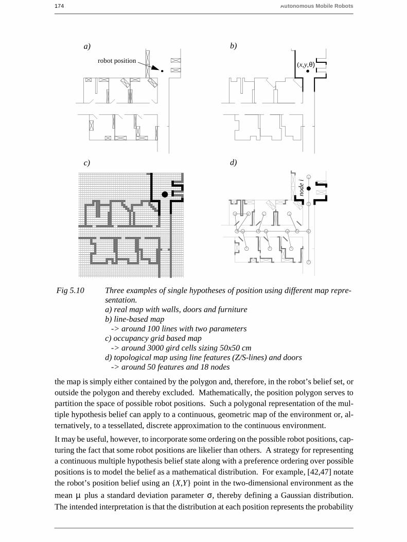
The single hypothesis belief representation is the most direct possible postulation of mobilerobot position. Given some environmental map, the robot’s belief about position is ex-pressed as a single unique point on the map. In Fig. 5.10, three examples of a single hypoth-esis belief are shown using three different map representations of the same actualenvironment (fig. 5.10a). In 5.10b, a single point is geometrically annotated as the robot’sposition in a continuous two-dimensional geometric map. In 5.10c, the map is a discrete,tessellated map, and the position is noted at the same level of fidelity as the map cell size.In 5.10d, the map is not geometrical at all but abstract and topological. In this case, the sin-gle hypothesis of position involves identifying a single node i in the topological graph as therobot’s position.
The principal advantage of the single hypothesis representation of position stems from thefact that, given a unique belief, there is no position ambiguity. The unambiguous nature ofthis representation facilitates decision-making at the robot’s cognitive level (e.g. path plan-ning). The robot can simply assume that its belief is correct, and can then select its futureactions based on its unique position.
Just as decision-making is facilitated by a single-position hypothesis, so updating the robot’sbelief regarding position is also facilitated, since the single position must be updated by def-inition to a new, single position. The challenge with this position update approach, whichultimately is the principal disadvantage of single-hypothesis representation, is that robotmotion often induces uncertainty due to effectory and sensory noise. Therefore, forcing theposition update process to always generate a single hypothesis of position is challenging
5 Mobile Robot Localization 173
and, often, impossible.
5.4.2 Multiple Hypothesis Belief
In the case of multiple hypothesis beliefs regarding position, the robot tracks not just a singlepossible position but a possibly infinite set of positions.
In one simple example originating in the work of Jean-Claude Latombe [5, 89], the robot’sposition is described in terms of a convex polygon positioned in a two-dimensional map ofthe environment. This multiple hypothesis representation communicates the set of possiblerobot positions geometrically, with no preference ordering over the positions. Each point in
Fig 5.9 Belief representation regarding the robot position (1 dimensional) in con-tinuous and discretized (tessellated) maps.a)Continuous map with multiple hypothesis belief, e.g. single Gaussian cen-tered at a single continuous valueb)Continuous map with multiple hypothesis belief, e.g. multiple Gaussianscentered at multiple continuous valuesc)Discretized (decomposed) grid map with probability values for all possi-ble robot position, e.g. Markov approachd)Discretized topological map with probability value for all possible nodes(topological robot positions), e.g. Markov approach
position x
prob
abili
tyP
position x
prob
abili
tyP
position x
prob
abili
tyP
a
b
c
node
prob
abili
tyP
d
A B C D E F G
of topological map
R. Siegwart, EPFL, Illah Nourbakhsh, CMU
174 Autonomous Mobile Robots
the map is simply either contained by the polygon and, therefore, in the robot’s belief set, oroutside the polygon and thereby excluded. Mathematically, the position polygon serves topartition the space of possible robot positions. Such a polygonal representation of the mul-tiple hypothesis belief can apply to a continuous, geometric map of the environment or, al-ternatively, to a tessellated, discrete approximation to the continuous environment.
It may be useful, however, to incorporate some ordering on the possible robot positions, cap-turing the fact that some robot positions are likelier than others. A strategy for representinga continuous multiple hypothesis belief state along with a preference ordering over possiblepositions is to model the belief as a mathematical distribution. For example, [42,47] notatethe robot’s position belief using an {X,Y} point in the two-dimensional environment as the
mean plus a standard deviation parameter , thereby defining a Gaussian distribution.
The intended interpretation is that the distribution at each position represents the probability
Fig 5.10 Three examples of single hypotheses of position using different map repre-sentation.a) real map with walls, doors and furnitureb) line-based map
-> around 100 lines with two parametersc) occupancy grid based map
-> around 3000 gird cells sizing 50x50 cmd) topological map using line features (Z/S-lines) and doors
-> around 50 features and 18 nodes
node
i
a)
c)
b)
d)
(x,y,θ)robot position
µ σ

5 Mobile Robot Localization 175
assigned to the robot being at that location. This representation is particularly amenable tomathematically defined tracking functions, such as the Kalman Filter, that are designed tooperate efficiently on Gaussian distributions.
An alternative is to represent the set of possible robot positions, not using a single Gaussianprobability density function, but using discrete markers for each possible position. In thiscase, each possible robot position is individually noted along with a confidence or probabil-ity parameter (See Fig. (5.11)). In the case of a highly tessellated map this can result in thou-sands or even tens of thousands of possible robot positions in a single belief state.
The key advantage of the multiple hypothesis representation is that the robot can explicitlymaintain uncertainty regarding its position. If the robot only acquires partial information re-garding position from its sensors and effectors, that information can conceptually be incor-porated in an updated belief.
A more subtle advantage of this approach revolves around the robot’s ability to explicitlymeasure its own degree of uncertainty regarding position. This advantage is the key to aclass of localization and navigation solutions in which the robot not only reasons aboutreaching a particular goal, but reasons about the future trajectory of its own belief state. Forinstance, a robot may choose paths that minimize its future position uncertainty. An exam-ple of this approach is [90], in which the robot plans a path from point A to B that takes itnear a series of landmarks in order to mitigate localization difficulties. This type of explicitreasoning about the effect that trajectories will have on the quality of localization requires amultiple hypothesis representation.
One of the fundamental disadvantages of the multiple hypothesis approaches involves deci-sion-making. If the robot represents its position as a region or set of possible positions, thenhow shall it decide what to do next? Figure 5.11 provides an example. At position 3, therobot’s belief state is distributed among 5 hallways separately. If the goal of the robot is totravel down one particular hallway, then given this belief state what action should the robotchoose?
The challenge occurs because some of the robot’s possible positions imply a motion trajec-
Fig 5.11 Example of multiple hypothesis tracking (courtesy of W. Burgard [43]). Thebelief state that is largely distributed becomes very certain after moving toposition 4
Belief states at positions 2, 3 and 4Path of the robot
R. Siegwart, EPFL, Illah Nourbakhsh, CMU

176 Autonomous Mobile Robots
tory that is inconsistent with some of its other possible positions. One approach that we willsee in the case studies below is to assume, for decision-making purposes, that the robot isphysically at the most probable location in its belief state, then to choose a path based onthat current position. But this approach demands that each possible position have an asso-ciated probability.
In general, the right approach to such a decision-making problems would be to decide ontrajectories that eliminate the ambiguity explicitly. But this leads us to the second major dis-advantage of the multiple hypothesis approaches. In the most general case, they can be com-putationally very expensive. When one reasons in a three dimensional space of discretepossible positions, the number of possible belief states in the single hypothesis case is lim-ited to the number of possible positions in the 3D world. Consider this number to be N.When one moves to an arbitrary multiple hypothesis representation, then the number of pos-
sible belief states is the power set of N, which is far larger: . Thus explicit reasoning
about the possible trajectory of the belief state over time quickly becomes computationallyuntenable as the size of the environment grows.
There are, however, specific forms of multiple hypothesis representations that are somewhatmore constrained, thereby avoiding the computational explosion while allowing a limitedtype of multiple hypothesis belief. For example, if one assumes a Gaussian distribution ofprobability centered at a single position, then the problem of representation and tracking ofbelief becomes equivalent to Kalman Filtering, a straightforward mathematical process de-scribed below. Alternatively, a highly tessellated map representation combined with a limitof 10 possible positions in the belief state, results in a discrete update cycle that is, at worst,only 10x more computationally expensive than single hypothesis belief update.
In conclusion, the most critical benefit of the multiple hypothesis belief state is the ability tomaintain a sense of position while explicitly annotating the robot’s uncertainty about its ownposition. This powerful representation has enabled robots with limited sensory informationto navigate robustly in an array of environments, as we shall see in the case studies below.
2N
5 Mobile Robot Localization 177
5.5 Map Representation
The problem of representing the environment in which the robot moves is a dual of the prob-lem of representing the robot’s possible position or positions. Decisions made regarding theenvironmental representation can have impact on the choices available for robot positionrepresentation. Often the fidelity of the position representation is bounded by the fidelity ofthe map.
Three fundamental relationships must be understood when choosing a particular map repre-sentation:
• The precision of the map must appropriately match the precision with which the ro-bot needs to achieve its goals.
• The precision of the map and the type of features represented must match the preci-sion and data types returned by the robot’s sensors.
• The complexity of the map representation has direct impact on the computationalcomplexity of reasoning about mapping, localization and navigation.
In the following sections, we identify and discuss critical design choices in creating a maprepresentation. Each such choice has great impact on the relationships listed above and onthe resulting robot localization architecture. As we will see, the choice of possible map rep-resentations is broad. Selecting an appropriate representation requires understanding all ofthe trade-offs inherent in that choice as well as understanding the specific context in whicha particular mobile robot implementation must perform localization. In general, the environ-ment representation and model can be roughly classified as presented in chapter 4.3.
5.5.1 Continuous Representations
A continuous-valued map is one method for exact decomposition of the environment. Theposition of environmental features can be annoted precisely in continuous space. Mobile ro-bot implementations to date use continuous maps only in two dimensional representations,as further dimensionality can result in computational explosion.
A common approach is to combine the exactness of a continuous representation with thecompactness of the closed world assumption. This means that one assumes that the repre-sentation will specify all environmental objects in the map, and that any area in the map thatis devoid of objects has no objects in the corresponding portion of the environment. Thus,the total storage needed in the map is proportional to the density of objects in the environ-ment, and a sparse environment can be represented by a low-memory map.
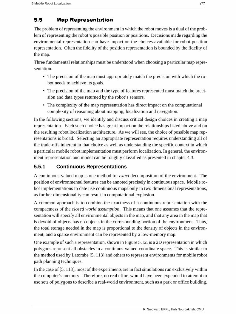
One example of such a representation, shown in Figure 5.12, is a 2D representation in whichpolygons represent all obstacles in a continuos-valued coordinate space. This is similar tothe method used by Latombe [5, 113] and others to represent environments for mobile robotpath planning techniques.
In the case of [5, 113], most of the experiments are in fact simulations run exclusively withinthe computer’s memory. Therefore, no real effort would have been expended to attempt touse sets of polygons to describe a real-world environment, such as a park or office building.
R. Siegwart, EPFL, Illah Nourbakhsh, CMU

178 Autonomous Mobile Robots
In other work in which real environments must be captured by the maps, one sees a trendtoward selectivity and abstraction. The human map-maker tends to capture on the map, forlocalization purposes, only objects that can be detected by the robot’s sensors and, further-more, only a subset of the features of real-world objects.
It should be immediately apparent that geometric maps can capably represent the physicallocations of objects without referring to their texture, color, elasticity, or any other such sec-ondary features that do not related directly to position and space. In addition to this level ofsimplification, a mobile robot map can further reduce memory usage by capturing only as-pects of object geometry that are immediately relevant to localization. For example all ob-jects may be approximated using very simple convex polygons, sacrificing map felicity forthe sake of computational speed.
One excellent example involves line extraction. Many indoor mobile robots rely upon laserrangefinding devices to recover distance readings to nearby objects. Such robots can auto-matically extract best-fit lines from the dense range data provided by thousands of points oflaser strikes. Given such a line extraction sensor, an appropriate continuous mapping ap-proach is to populate the map with a set of infinite lines. The continuous nature of the mapguarantees that lines can be positioned at arbitrary positions in the plane and at arbitrary an-gles. The abstraction of real environmental objects such as walls and intersections capturesonly the information in the map representation that matches the type of information recov-ered by the mobile robot’s rangefinding sensor.
Figure 5.13 shows a map of an indoor environment at EPFL using a continuous line repre-
Fig 5.12 A continous representation using polygons as environmental obstacles

5 Mobile Robot Localization 179
sentation. Note that the only environmental features captured by the map are straight lines,such as those found at corners and along walls. This represents not only a sampling of thereal world of richer features, but also a simplification, for an actual wall may have textureand relief that is not captured by the mapped line.
The impact of continuos map representations on position representation is primarily posi-tive. In the case of single hypothesis position representation, that position may be specifiedas any continuous-valued point in the coordinate space, and therefore extremely high accu-racy is possible. In the case of multiple hypothesis position representation, the continuousmap enables two types of multiple position representation.
In one case, the possible robot position may be depicted as a geometric shape in the hyper-plane, such that the robot is known to be within the bounds of that shape. This is shown inFigure 5.30, in which the position of the robot is depicted by an oval bounding area.
Yet, the continuous representation does not disallow representation of position in the formof a discrete set of possible positions. For instance, in [111] the robot position belief stateis captured by sampling nine continuous-valued positions from within a region near the ro-bot’s best known position. This algorithm captures, within a continuous space, a discretesampling of possible robot positions.
In summary, the key advantage of a continuous map representation is the potential for highaccuracy and expressiveness with respect to the environmental configuration as well as therobot position within that environment. The danger of a continuous representation is thatthe map may be computationally costly. But this danger can be tempered by employing ab-straction and capturing only the most relevant environmental features. Together with theuse of the closed world assumption, these techniques can enable a continuous-valued mapto be no more costly, and sometimes even less costly, than a standard discrete representation.
5.5.2 Decomposition Strategies
In the section above, we discussed one method of simplification, in which the continuousmap representation contains a set of infinite lines that approximate real-world environmentallines based on a two-dimensional slice of the world. Basically this transformation from thereal world to the map representation is a filter that removes all non-straight data and further-more extends line segment data into infinite lines that require fewer parameters.
Fig 5.13 Example of a continuous-valued line representation of EPFL.left: real mapright: representation with a set of infinite lines
R. Siegwart, EPFL, Illah Nourbakhsh, CMU
180 Autonomous Mobile Robots
A more dramatic form of simplification is abstraction: a general decomposition and selec-tion of environmental features. In this section, we explore decomposition as applied in itsmore extreme forms to the question of map representation.
Why would one radically decompose the real environment during the design of a map rep-resentation? The immediate disadvantage of decomposition and abstraction is the loss offidelity between the map and the real world. Both qualitatively, in terms of overall structure,and quantitatively, in terms of geometric precision, a highly abstract map does not comparefavorably to a high-fidelity map.
Despite this disadvantage, decomposition and abstraction may be useful if the abstractioncan be planned carefully so as to capture the relevant, useful features of the world while dis-carding all other features. The advantage of this approach is that the map representation canpotentially be minimized. Furthermore, if the decomposition is hierarchical, such as in apyramid of recursive abstraction, then reasoning and planning with respect to the map rep-resentation may be computationally far superior to planning in a fully detailed world model.
A standard, lossless form of opportunistic decomposition is termed exact cell decomposi-tion. This method, introduced by [5], achieves decomposition by selecting boundaries be-tween discrete cells based on geometric criticality.
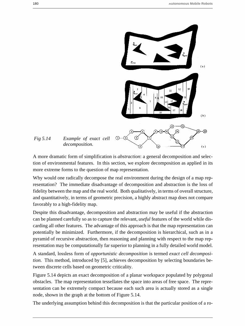
Figure 5.14 depicts an exact decomposition of a planar workspace populated by polygonalobstacles. The map representation tessellates the space into areas of free space. The repre-sentation can be extremely compact because each such area is actually stored as a singlenode, shown in the graph at the bottom of Figure 5.14.
The underlying assumption behind this decomposition is that the particular position of a ro-
Fig 5.14 Example of exact celldecomposition.
5 Mobile Robot Localization 181
bot within each area of free space does not matter. What matters is the robot’s ability totraverse from each area of free space to the adjacent areas. Therefore, as with other repre-sentations we will see, the resulting graph captures the adjacency of map locales. If indeedthe assumptions are valid and the robot does not care about its precise position within a sin-gle area, then this can be an effective representation that nonetheless captures the connec-tivity of the environment.
Such an exact decomposition is not always appropriate. Exact decomposition is a functionof the particular environment obstacles and free space. If this information is expensive tocollect or even unknown, then such an approach is not feasible.
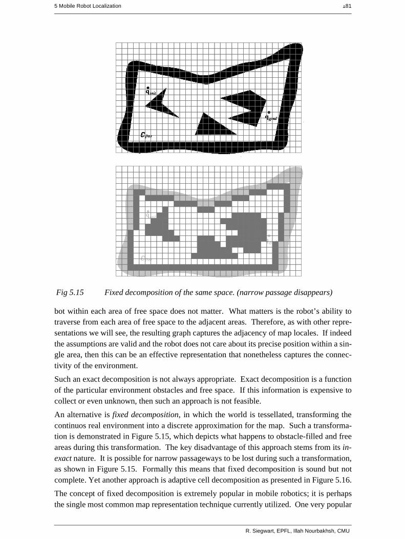
An alternative is fixed decomposition, in which the world is tessellated, transforming thecontinuos real environment into a discrete approximation for the map. Such a transforma-tion is demonstrated in Figure 5.15, which depicts what happens to obstacle-filled and freeareas during this transformation. The key disadvantage of this approach stems from its in-exact nature. It is possible for narrow passageways to be lost during such a transformation,as shown in Figure 5.15. Formally this means that fixed decomposition is sound but notcomplete. Yet another approach is adaptive cell decomposition as presented in Figure 5.16.
The concept of fixed decomposition is extremely popular in mobile robotics; it is perhapsthe single most common map representation technique currently utilized. One very popular
Fig 5.15 Fixed decomposition of the same space. (narrow passage disappears)
R. Siegwart, EPFL, Illah Nourbakhsh, CMU

182 Autonomous Mobile Robots
version of fixed decomposition is known as the occupancy grid representation [91]. In anoccupancy grid, the environment is represented by a discrete grid, where each cell is eitherfilled (part of an obstacle) or empty (part of free space). This method is of particular valuewhen a robot is equipped with range-based sensors because the range values of each sensor,combined with the absolute position of the robot, can be used directly to update the filled/empty value of each cell.
In the occupancy grid, each cell may have a counter, whereby the value 0 indicates that thecell has not been "hit" by any ranging measurements and, therefore, it is likely free space.As the number of ranging strikes increases, the cell’s value is incremented and, above a cer-tain threshold, the cell is deemed to be an obstacle. By discounting the values of cells overtime, both hysteresis and the possibility of transient obstacles can be represented using thisoccupancy grid approach. Figure 5.17 depicts an occupancy grid representation in whichthe darkness of each cell is proportional to the value of its counter. One commercial robotthat uses a standard occupancy grid for mapping and navigation is the Cye robot [112].
Fig 5.16 Example of adaptive decomposition of an environment.
Fig 5.17 Example of an occupancy grid map representation.

5 Mobile Robot Localization 183
There remain two main disadvantages of the occupancy grid approach. First, the size of themap in robot memory grows with the size of the environment and, if a small cell size is used,this size can quickly become untenable. This occupancy grid approach is not compatiblewith the closed world assumption, which enabled continuous representations to have poten-tially very small memory requirements in large, sparse environments. In contrast, the occu-pancy grid must have memory set aside for every cell in the matrix. Furthermore, any fixeddecomposition method such as this imposes a geometric grid on the world a priori, regard-less of the environmental details. This can be inappropriate in cases where geometry is notthe most salient feature of the environment.
For these reasons, an alternative, called topological decomposition, has been the subject ofsome exploration in mobile robotics. Topological approaches avoid direct measurement ofgeometric environmental qualities, instead concentrating on characteristics of the environ-ment that are most relevant to the robot for localization.
Formally, a topological representation is a graph that specifies two things: nodes and theconnectivity between those nodes. Insofar as a topological representation is intended for theuse of a mobile robot, nodes are used to denote areas in the world and arcs are used to denoteadjacency of pairs of nodes. When an arc connects two nodes, then the robot can traversefrom one node to the other without requiring traversal of any other intermediary node.
Adjacency is clearly at the heart of the topological approach, just as adjacency in a cell de-composition representation maps to geometric adjacency in the real world. However, thetopological approach diverges in that the nodes are not of fixed size nor even specificationsof free space. Instead, nodes document an area based on any sensor discriminant such thatthe robot can recognize entry and exit of the node.
Figure 5.18 depicts a topological representation of a set of hallways and offices in an indoor
Fig 5.18 A topological representation of an indoor office area.
1
2
3
4
5
6
7
8
9
10
11
12
13
14
15
16
18 17
R. Siegwart, EPFL, Illah Nourbakhsh, CMU
184 Autonomous Mobile Robots
environment. In this case, the robot is assumed to have an intersection detector, perhaps us-ing sonar and vision to find intersections between halls and between halls and rooms. Notethat nodes capture geometric space and arcs in this representation simply represent connec-tivity.
Another example of topological representation is the work of Dudek [49], in which the goalis to create a mobile robot that can capture the most interesting aspects of an area for humanconsumption. The nodes in Dudek’s representation are visually striking locales rather thanroute intersections.
In order to navigate using a topological map robustly, a robot must satisfy two constraints.First, it must have a means for detecting its current position in terms of the nodes of the to-pological graph. Second, it must have a means for traveling between nodes using robot mo-tion. The node sizes and particular dimensions must be optimized to match the sensorydiscrimination of the mobile robot hardware. This ability to "tune" the representation to therobot’s particular sensors can be an important advantage of the topological approach. How-ever, as the map representation drifts further away from true geometry, the expressivenessof the representation for accurately and precisely describing a robot position is lost. Thereinlies the compromise between the discrete cell-based map representations and the topologicalrepresentations. Interestingly, the continuous map representation has the potential to beboth compact like a topological representation and precise as with all direct geometric rep-resentations.
Yet, a chief motivation of the topological approach is that the environment may contain im-portant non-geometric features - features that have no ranging relevance but are useful forlocalization. In Chapter 4 we described such whole-image vision-based features.
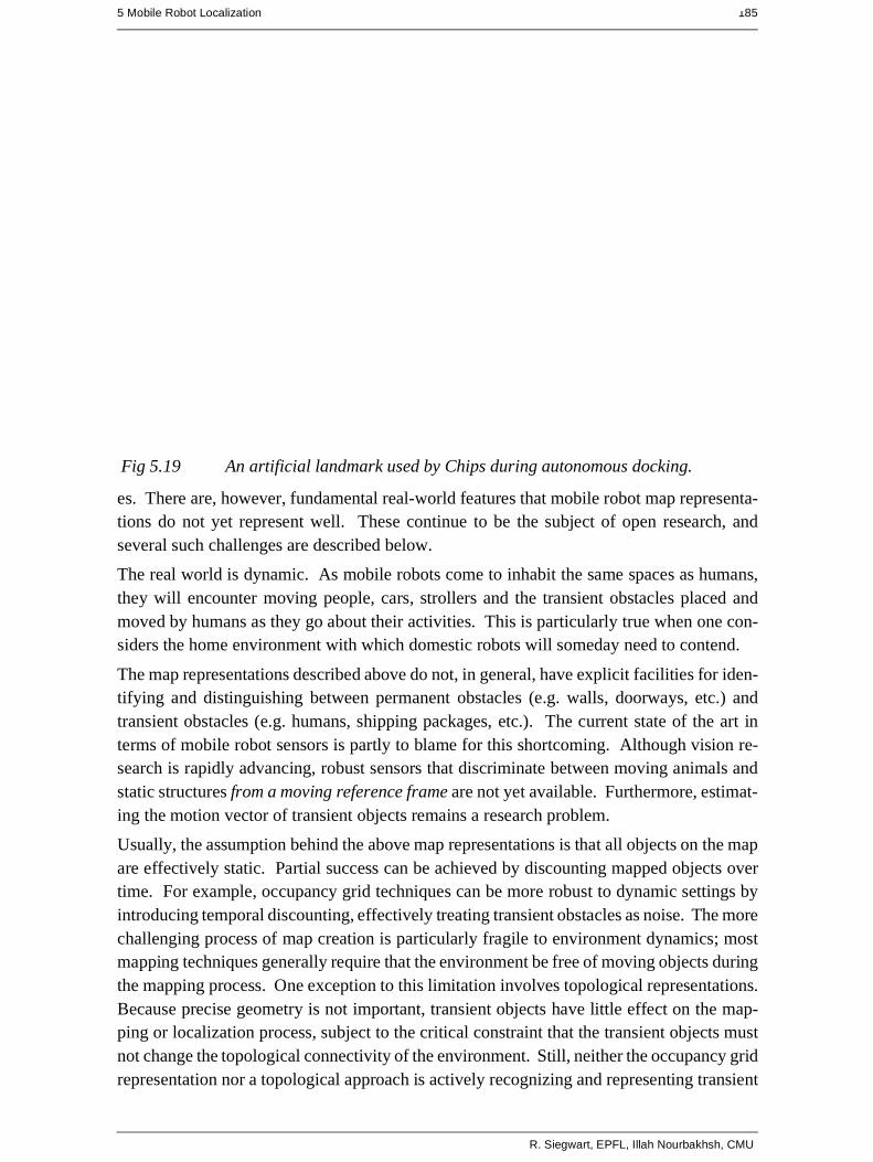
In contrast to these whole-image feature extractors, often spatially localized landmarks areartificially placed in an environment to impose a particular visual-topological connectivityupon the environment. In effect, the artificial landmark can impose artificial structure. Ex-amples of working systems operating with this landmark-based strategy have also demon-strated success. Latombe’s landmark-based navigation research [89] has been implementedon real-world indoor mobile robots that employ paper landmarks attached to the ceiling asthe locally observable features. Chips the museum robot is another robot that uses man-made landmarks to obviate the localization problem. In this case, a bright pink square servesas a landmark with dimensions and color signature that would be hard to accidentally repro-duce in a museum environment [88]. One such museum landmark is shown in Figure (5.19).
In summary, range is clearly not the only measurable and useful environmental value for amobile robot. This is particularly true due to the advent of color vision as well as laserrangefinding, which provides reflectance information in addition to range information.Choosing a map representation for a particular mobile robot requires first understanding thesensors available on the mobile robot and second understanding the mobile robot’s function-al requirements (e.g. required goal precision and accuracy).
5.5.3 State of the Art: Current Challenges in Map Representation
The sections above describe major design decisions in regards to map representation choic-
5 Mobile Robot Localization 185
es. There are, however, fundamental real-world features that mobile robot map representa-tions do not yet represent well. These continue to be the subject of open research, andseveral such challenges are described below.
The real world is dynamic. As mobile robots come to inhabit the same spaces as humans,they will encounter moving people, cars, strollers and the transient obstacles placed andmoved by humans as they go about their activities. This is particularly true when one con-siders the home environment with which domestic robots will someday need to contend.
The map representations described above do not, in general, have explicit facilities for iden-tifying and distinguishing between permanent obstacles (e.g. walls, doorways, etc.) andtransient obstacles (e.g. humans, shipping packages, etc.). The current state of the art interms of mobile robot sensors is partly to blame for this shortcoming. Although vision re-search is rapidly advancing, robust sensors that discriminate between moving animals andstatic structures from a moving reference frame are not yet available. Furthermore, estimat-ing the motion vector of transient objects remains a research problem.
Usually, the assumption behind the above map representations is that all objects on the mapare effectively static. Partial success can be achieved by discounting mapped objects overtime. For example, occupancy grid techniques can be more robust to dynamic settings byintroducing temporal discounting, effectively treating transient obstacles as noise. The morechallenging process of map creation is particularly fragile to environment dynamics; mostmapping techniques generally require that the environment be free of moving objects duringthe mapping process. One exception to this limitation involves topological representations.Because precise geometry is not important, transient objects have little effect on the map-ping or localization process, subject to the critical constraint that the transient objects mustnot change the topological connectivity of the environment. Still, neither the occupancy gridrepresentation nor a topological approach is actively recognizing and representing transient
Fig 5.19 An artificial landmark used by Chips during autonomous docking.
R. Siegwart, EPFL, Illah Nourbakhsh, CMU
186 Autonomous Mobile Robots
objects as distinct from both sensor error and permanent map features.
As vision sensing provides more robust and more informative content regarding the tran-sience and motion details of objects in the world, mobile roboticists will in time propose rep-resentations that make use of that information. A classic example involves occlusion byhuman crowds. Museum tour guide robots generally suffer from an extreme amount of oc-clusion. If the robot’s sensing suite is located along the robot’s body, then the robot is ef-fectively blind when a group of human visitors completely surrounds the robot. This isbecause its map contains only environment features that are, at that point, fully hidden fromthe robot’s sensors by the wall of people. In the best case, the robot should recognize itsocclusion and make no effort to localize using these invalid sensor readings. In the worstcase, the robot will localize with the fully occluded data, and will update its location incor-rectly. A vision sensor that can discriminate the local conditions of the robot (e.g. we aresurrounded by people) can help eliminate this error mode.
A second open challenge in mobile robot localization involves the traversal of open spaces.Existing localization techniques generally depend on local measures such as range, therebydemanding environments that are somewhat densely filled with objects that the sensors candetect and measure. Wide open spaces such as parking lots, fields of grass and indoor atri-ums such as those found in convention centers pose a difficulty for such systems due to theirrelative sparseness. Indeed, when populated with humans, the challenge is exacerbated be-cause any mapped objects are almost certain to be occluded from view by the people.
Once again, more recent technologies provide some hope for overcoming these limitations.Both vision and state-of-the-art laser rangefinding devices offer outdoor performance withranges of up to a hundred meters and more. Of course, GPS performs even better. Suchlong-range sensing may be required for robots to localize using distant features.
This trend teases out a hidden assumption underlying most topological map representations.Usually, topological representations make assumptions regarding spatial locality: a nodecontains objects and features that are themselves within that node. The process of map cre-ation thus involves making nodes that are, in their own self-contained way, recognizable byvirtue of the objects contained within the node. Therefore, in an indoor environment, eachroom can be a separate node, and this is reasonable because each room will have a layoutand a set of belongings that are unique to that room.
However, consider the outdoor world of a wide-open park. Where should a single node endand the next node begin? The answer is unclear because objects that are far away from thecurrent node, or position, can yield information for the localization process. For example,the hump of a hill at the horizon, the position of a river in the valley and the trajectory of thesun all are non-local features that have great bearing on one’s ability to infer current posi-tion. The spatial locality assumption is violated and, instead, replaced by a visibility crite-rion: the node or cell may need a mechanism for representing objects that are measurableand visible from that cell. Once again, as sensors improve and, in this case, as outdoor lo-comotion mechanisms improve, there will be greater urgency to solve problems associatedwith localization in wide-open settings, with and without GPS-type global localization sen-sors.
5 Mobile Robot Localization 187
We end this section with one final open challenge that represents one of the fundamental ac-ademic research questions of robotics: sensor fusion. A variety of measurement types arepossible using off-the-shelf robot sensors, including heat, range, acoustic and light-based re-flectivity, color, texture, friction, etc. Sensor fusion is a research topic closely related to maprepresentation. Just as a map must embody an environment in sufficient detail for a robotto perform localization and reasoning, sensor fusion demands a representation of the worldthat is sufficiently general and expressive that a variety of sensor types can have their datacorrelated appropriately, strengthening the resulting percepts well beyond that of any indi-vidual sensor’s readings.
Perhaps the only general implementation of sensor fusion to date is that of neural networkclassifier. Using this technique, any number and any type of sensor values may be jointlycombined in a network that will use whatever means necessary to optimize its classificationaccuracy. For the mobile robot that must use a human-readable internal map representation,no equally general sensor fusion scheme has yet been born. It is reasonable to expect that,when the sensor fusion problem is solved, integration of a large number of disparate sensortypes may easily result in sufficient discriminatory power for robots to achieve real-worldnavigation, even in wide-open and dynamic circumstances such as a public square filledwith people.
R. Siegwart, EPFL, Illah Nourbakhsh, CMU

188 Autonomous Mobile Robots
5.6 Probabilistic Map-Based Localization
5.6.1 Introduction
As stated earlier, multiple hypothesis position representation is advantageous because therobot can explicitly track its own beliefs regarding its possible positions in the environment.Ideally, the robot’s belief state will change, over time, as is consistent with its motor outputsand perceptual inputs. One geometric approach to multiple hypothesis representation, men-tioned earlier, involves identifying the possible positions of the robot by specifying a poly-gon in the environmental representation [113]. This method does not provide any indicationof the relative chances between various possible robot positions.
Probabilistic techniques differ from this because they explicitly identify probabilities withthe possible robot positions, and for this reason these methods have been the focus of recentresearch. In the following sections we present two classes of probabilistic localization. Thefirst class, Markov localization, uses an explicitly specified probability distribution acrossall possible robots positions. The second method, Kalman filter localization, uses a Gauss-ian probability density representation of robot position and scan matching for localization.Unlike Markov localization, Kalman filter localization does not independently considereach possible pose in the robot’s configuration space. Interestingly, the Kalman filter local-ization process results from the Markov localization axioms if the robot’s position uncer-tainty is assumed to have a Gaussian form [28 page 43-44].
Before discussing each method in detail, we present the general robot localization problemand solution strategy. Consider a mobile robot moving in a known environment. As it startsto move, say from a precisely known location, it can keep track of its motion using odome-try. Due to odometry uncertainty, after some movement the robot will become very uncer-tain about its position (see section 5.2.4). To keep position uncertainty from growingunbounded, the robot must localize itself in relation to its environment map. To localize, therobot might use its on-board sensors (ultrasonic, range sensor, vision) to make observationsof its environment. The information provided by the robot’s odometry, plus the informationprovided by such exteroceptive observations can be combined to enable the robot to localizeas well as possible with respect to its map. The processes of updating based on propriocep-tive sensor values and exteroceptive sensor values are often separated logically, leading toa general two-step process for robot position update.
Action update represents the application of some action model Act to the mobile robot’s
proprioceptive encoder measurements and prior belief state to yield a new belief
state representing the robot’s belief about its current position. Note that throughout thischapter we will assume that the robot’s proprioceptive encoder measurements are used asthe best possible measure of its actions over time. If, for instance, a differential drive robothad motors without encoders connected to its wheels and employed open-loop control, theninstead of encoder measurements the robot’s highly uncertain estimates of wheel spin wouldneed to be incorporated. We ignore such cases and therefore have a simple formula:
. (5.16)
ot st 1–
s't Act ot st 1–,( )=
5 Mobile Robot Localization 189
Perception update represents the application of some perception model See to the mobile
robot’s exteroceptive sensor inputs and updated belief state to yield a refined belief
state representing the robot’s current position:
(5.17)
The perception model See and sometimes the action model Act are abstract functions of boththe map and the robot’s physical configuration (e.g. sensors and their positions, kinematics,etc.).
In general, the action update process contributes uncertainty to the robot’s belief about po-sition: encoders have error and therefore motion is somewhat nondeterministic. By contrast,perception update generally refines the belief state. Sensor measurements, when comparedto the robot’s environmental model, tend to provide clues regarding the robot’s possible po-sition.
In the case of Markov localization, the robot’s belief state is usually represented as separateprobability assignments for every possible robot pose in its map. The action update and per-ception update processes must update the probability of every cell in this case. Kalman filterlocalization represents the robot’s belief state using a singe, well-defined Gaussian proba-
bility density function, and thus retains just a and parameterization of the robot’s belief
about position with respect to the map. Updating the parameters of the Gaussian distributionis all that is required. This fundamental difference in the representation of belief state leadsto the following advantages and disadvantages of the two methods, as presented in [44]:
• Markov localization allows for localization starting from any unknown position andcan thus recover from ambiguous situations because the robot can track multiple,completely disparate possible positions. However, to update the probability of allpositions within the whole state space at any time requires a discrete representationof the space (grid). The required memory and computational power can thus limitprecision and map size.
• Kalman filter localization tracks the robot from an initially known position and is in-herently both precise and efficient. In particular, Kalman filter localization can beused in continuous world representations. However, if the uncertainty of the robotbecomes too large (e.g. due to a robot collision with an object) and thus not truly un-imodal, the Kalman filter can fail to capture the multitude of possible robot positionsand can become irrevocably lost.
In recent research projects improvements are achieved or proposed by either only updatingthe state space of interest within the Markov approach [43] or by combining both methodsto create a hybrid localization system [44]. In the next two subsections we will present eachapproach in detail.
5.6.2 Markov Localization (see also [42, 45, 71, 72])
Markov localization tracks the robot’s belief state using an arbitrary probability densityfunction to represent the robot’s position. In practice, all known Markov localization sys-
it s't
st See it s't,( )=
µ σ
R. Siegwart, EPFL, Illah Nourbakhsh, CMU

190 Autonomous Mobile Robots
tems implement this generic belief representation by first tessellating the robot configurationspace into a finite, discrete number of possible robot poses in the map. In actual applica-tions, the number of possible poses can range from several hundred positions to millions ofpositions.
Given such a generic conception of robot position, a powerful update mechanism is requiredthat can compute the belief state that results when new information (e.g. encoder values andsensor values) is incorporated into a prior belief state with arbitrary probability density. Thesolution is born out of probability theory, and so the next section describes the foundationsof probability theory that apply to this problem, notably Bayes formula. Then, two subse-quent subsections provide case studies, one robot implementing a simple feature-driven to-pological representation of the environment [45, 71, 72] and the other using a geometricgrid-based map[42, 43].
5.6.2.1 Introduction: applying probability theory to robot localization
Given a discrete representation of robot positions, in order to express a belief state we wishto assign to each possible robot position a probability that the robot is indeed at that position.From probability theory we use the term p(A) to denote the probability that A is true. Thisis also called the prior probability of A because it measures the probability that A is true in-
dependent of any additional knowledge we may have. For example we can use to
denote the prior probability that the robot r is at position l at time t.
In practice, we wish to compute the probability of each individual robot position given theencoder and sensor evidence the robot has collected. In probability theory, we use the termp(A|B) to denote the conditional probability of A given that we know B. For example, we
use to denote the probability that the robot is at position l given that the robot’s
sensor inputs i.
The question is, how can a term such as be simplified to its constituent parts so
that it can be computed? The answer lies in the product rule, which states:
(5.18)
Equation 5.18 is intuitively straightforward, as the probability of both A and B being true isbeing related to B being true and the other being conditionally true. But you should be ableto convince yourself that the alternate equation is equally correct:
(5.19)
Using Equations 5.18 and 5.19 together, we can derive Bayes formula for computing p(A|B):
(5.20)
We use Bayes rule to compute the robot’s new belief state as a function of its sensory inputs
p rt l=( )
p rt l it=( )
p rt l it=( )
p A B∧( ) p A B( )p B( )=
p A B∧( ) p B A( )p A( )=
p A B( )p B A( )p A( )
p B( )------------------------------=

5 Mobile Robot Localization 191
and its former belief state. But to do this properly, we must recall the basic goal of the Mark-ov localization approach: a discrete set of possible robot positions L are represented. The
belief state of the robot must assign a probability for each location l in L.
The See function described in Equation 5.17 expresses a mapping from a belief state andsensor input to a refined belief state. To do this, we must update the probability associatedwith each position l in L, and we can do this by directly applying Bayes formula to everysuch l. In denoting this, we will stop representing the temporal index t for simplicity andwill further use p(l) to mean p(r=l):
(5.21)
The value of p(i|l) is key to Equation 5.21, and this probability of a sensor input at each robotposition must be computed using some model. An obvious strategy would be to consult therobot’s map, identifying the probability of particular sensor readings with each possible mapposition, given knowledge about the robot’s sensor geometry and the mapped environment.The value of p(l) is easy to recover in this case. It is simply the probability p(r=l) associatedwith the belief state before the perceptual update process. Finally, note that the denominatorp(i) does not depend upon l; that is, as we apply Equation 5.21 to all positions l in L, thedenominator never varies. Because it is effectively constant, in practice this denominator isusually dropped and, at the end of the perception update step, all probabilities in the beliefstate are re-normalized to sum at 1.0.
Now consider the Act function of Equation 5.16. Act maps a former belief state and encodermeasurement (i.e. robot action) to a new belief state. In order to compute the probability ofposition l in the new belief state, one must integrate over all the possible ways in which therobot may have reached l according to the potential positions expressed in the former beliefstate. This is subtle but fundamentally important. The same location l can be reached frommultiple source locations with the same encoder measurement o because the encoder mea-surement is uncertain. Temporal indices are required in this update equation:
(5.22)
Thus, the total probability for a specific position l is built up from the individual contribu-
tions from every location in the former belief state given encoder measurement o.
Equations 5.21 and 5.22 form the basis of Markov localization, and they incorporate theMarkov assumption. Formally, this means that their output is a function only of the robot’sprevious state and its most recent actions (odometry) and perception. In a general, non-Markovian situation, the state of a system depends upon all of its history. After all, the valueof a robot’s sensors at time t do not really depend only on its position at time t. They dependto some degree on the trajectory of the robot over time; indeed on the entire history of therobot. For example, the robot could have experienced a serious collision recently that hasbiased the sensor’s behavior. By the same token, the position of the robot at time t does not
p rt l=( )
p l i( )p i l( )p l( )
p i( )------------------------=
p lt ot( ) p lt l't 1– ot,( )p l't 1–( ) l't 1–d∫=
l'
R. Siegwart, EPFL, Illah Nourbakhsh, CMU
192 Autonomous Mobile Robots
really depend only on its position at time t-1 and its odometric measurements. Due to itshistory of motion, one wheel may have worn more than the other, causing a left-turning biasover time that affects its current position.
So the Markov assumption is, of course, not a valid assumption. However the Markov as-sumption greatly simplifies tracking, reasoning and planning and so it is an approximationthat continues to be extremely popular in mobile robotics.
5.6.2.2 Case Study I: Markov Localization using a Topological Map
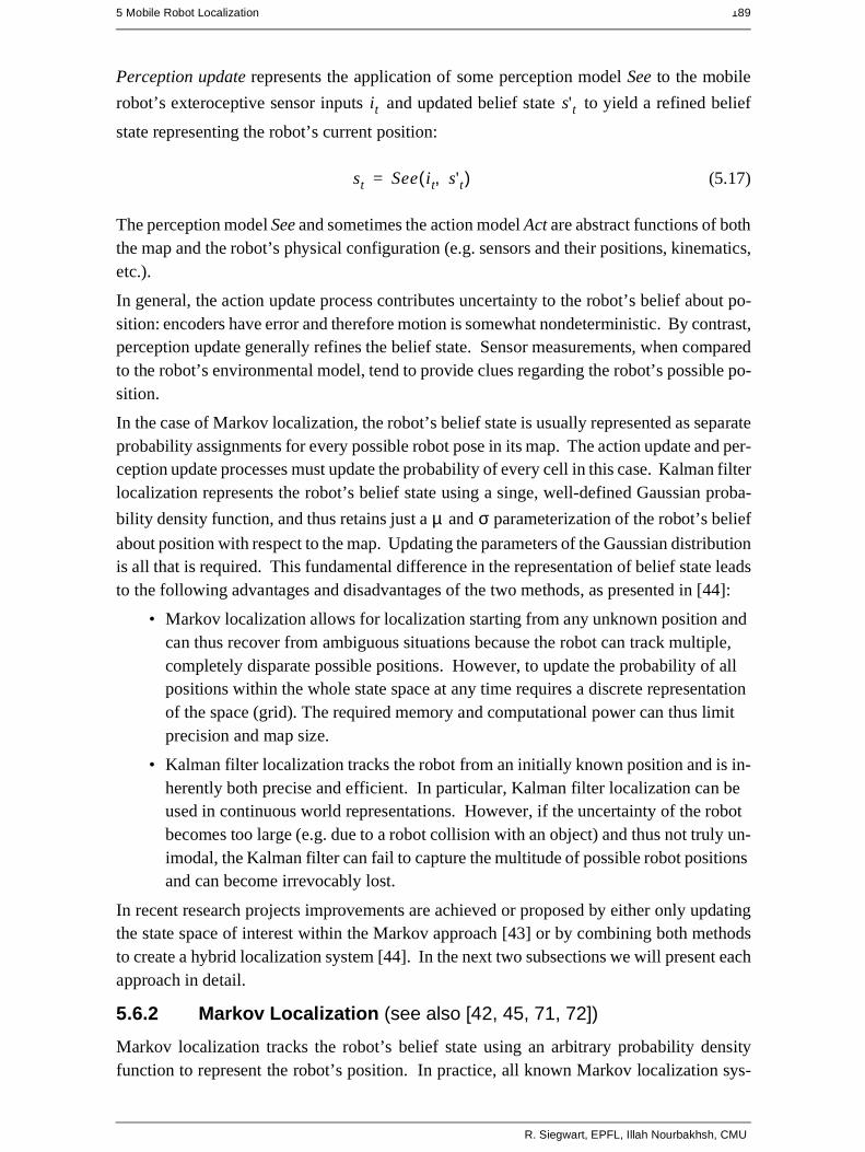
A straightforward application of Markov localization is possible when the robot’s environ-ment representation already provides an appropriate decomposition. This is the case whenthe environment representation is purely topological.
Consider a contest in which each robot is to receive a topological description of the environ-ment. The description would describe only the connectivity of hallways and rooms, with nomention of geometric distance. In addition, this supplied map would be imperfect, contain-ing several false arcs (e.g. a closed door). Such was the case for the 1994 AAAI NationalRobot Contest, at which each robot’s mission was to use the supplied map and its own sen-sors to navigate from a chosen starting position to a target room.
Dervish, the winner of this contest, employed probabilistic Markov localization and usedjust this multiple hypothesis belief state over a topological environmental representation.We now describe Dervish as an example of a robot with a topological representation and aprobabilistic localization algorithm.
Dervish, shown in Figure 5.20, includes a sonar arrangement custom-designed for the 1994AAAI National Robot Contest. The environment in this contest consisted of a rectilinearindoor office space filled with real office furniture as obstacles. Traditional sonars are ar-ranged radially around the robot in a ring. Robots with such sensor configurations are sub-ject to both tripping over short objects below the ring and to decapitation by tall objects(such as ledges, shelves and tables) that are above the ring.
Dervish’s answer to this challenge was to arrange one pair of sonars diagonally upward to
Fig 5.20 Dervish exploring its environment
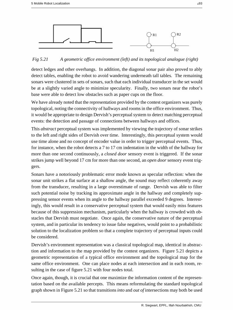
5 Mobile Robot Localization 193
detect ledges and other overhangs. In addition, the diagonal sonar pair also proved to ablydetect tables, enabling the robot to avoid wandering underneath tall tables. The remainingsonars were clustered in sets of sonars, such that each individual transducer in the set wouldbe at a slightly varied angle to minimize specularity. Finally, two sonars near the robot’sbase were able to detect low obstacles such as paper cups on the floor.
We have already noted that the representation provided by the contest organizers was purelytopological, noting the connectivity of hallways and rooms in the office environment. Thus,it would be appropriate to design Dervish’s perceptual system to detect matching perceptualevents: the detection and passage of connections between hallways and offices.
This abstract perceptual system was implemented by viewing the trajectory of sonar strikesto the left and right sides of Dervish over time. Interestingly, this perceptual system woulduse time alone and no concept of encoder value in order to trigger perceptual events. Thus,for instance, when the robot detects a 7 to 17 cm indentation in the width of the hallway formore than one second continuously, a closed door sensory event is triggered. If the sonarstrikes jump well beyond 17 cm for more than one second, an open door sensory event trig-gers.
Sonars have a notoriously problematic error mode known as specular reflection: when thesonar unit strikes a flat surface at a shallow angle, the sound may reflect coherently awayfrom the transducer, resulting in a large overestimate of range. Dervish was able to filtersuch potential noise by tracking its approximate angle in the hallway and completely sup-pressing sensor events when its angle to the hallway parallel exceeded 9 degrees. Interest-ingly, this would result in a conservative perceptual system that would easily miss featuresbecause of this suppression mechanism, particularly when the hallway is crowded with ob-stacles that Dervish must negotiate. Once again, the conservative nature of the perceptualsystem, and in particular its tendency to issue false negatives, would point to a probabilisticsolution to the localization problem so that a complete trajectory of perceptual inputs couldbe considered.
Dervish’s environment representation was a classical topological map, identical in abstrac-tion and information to the map provided by the contest organizers. Figure 5.21 depicts ageometric representation of a typical office environment and the topological map for thesame office environment. One can place nodes at each intersection and in each room, re-sulting in the case of figure 5.21 with four nodes total.
Once again, though, it is crucial that one maximize the information content of the represen-tation based on the available percepts. This means reformulating the standard topologicalgraph shown in Figure 5.21 so that transitions into and out of intersections may both be used
Fig 5.21 A geometric office environment (left) and its topological analogue (right)
R1 R2
H1 H2
R. Siegwart, EPFL, Illah Nourbakhsh, CMU

194 Autonomous Mobile Robots
for position updates. Figure 5.22 shows a modification of the topological map in which justthis step has been taken. In this case, note that there are 7 nodes in contrast to 4.
In order to represent a specific belief state, Dervish associated with each topological node n
a probability that the robot is at a physical position within the boundaries of n: .
As will become clear below, the probabilistic update used by Dervish was approximate,therefore technically one should refer to the resulting values as likelihoods rather than prob-abilities.
The perception update process for Dervish functions precisely as in Equation (5.21). Per-ceptual events are generated asynchronously, each time the feature extractor is able to rec-ognize a large-scale feature (e.g. doorway, intersection) based on recent ultrasonic values.Each perceptual event consists of a percept-pair (a feature on one side of the robot or twofeatures on both sides).
Given a specific percept pair i, Equation (5.21) enables the likelihood of each possible po-sition n to be updated using the formula:
(5.23)
The value of p(n) is already available from the current belief state of Dervish, and so thechallenge lies in computing p(i|n). The key simplification for Dervish is based upon the re-alization that, because the feature extraction system only extracts 4 total features and be-cause a node contains (on a single side) one of 5 total features, every possible combinationof node type and extracted feature can be represented in a 4 x 5 table.
Dervish’s certainty matrix (show in Table 5.1) is just this lookup table. Dervish makes thesimplifying assumption that the performance of the feature detector (i.e. the probability thatit is correct) is only a function of the feature extracted and the actual feature in the node.With this assumption in hand, we can populate the certainty matrix with confidence esti-
Table 5.1: Dervish’s certainty matrix.
Wall ClosedDoor
OpenDoor
OpenHallway
Foyer
Nothing detected 0.70 0.40 0.05 0.001 0.30
Closed door detected 0.30 0.60 0 0 0.05
Open door detected 0 0 0.90 0.10 0.15
Open hallway detected 0 0 0.001 0.90 0.50
Fig 5.22 A modification of the topological map to maximize information.
R1 R2
H1 H2H0-1 H1-2 H2-3
p rt n=( )
p n i( ) p i n( )p n( )=

5 Mobile Robot Localization 195
mates for each possible pairing of perception and node type. For each of the five world fea-tures that the robot can encounter (wall, closed door, open door, open hallway and foyer)this matrix assigns a likelihood for each of the three one-sided percepts that the sensory sys-tem can issue. In addition, this matrix assigns a likelihood that the sensory system will failto issue a perceptual event altogether (nothing detected).
For example, using the specific values in Table 5.1, if Dervish is next to an open hallway,the likelihood of mistakenly recognizing it as an open door is 0.10. This means that for anynode n that is of type Open Hallway and for the sensor value i=Open door, p(i|n) = 0.10.Together with a specific topological map, the certainty matrix enables straightforward com-putation of p(i|n) during the perception update process.
For Dervish’s particular sensory suite and for any specific environment it intends to navi-gate, humans generate a specific certainty matrix that loosely represents its perceptual con-fidence, along with a global measure for the probability that any given door will be closedversus opened in the real world.
Recall that Dervish has no encoders and that perceptual events are triggered asynchronouslyby the feature extraction processes. Therefore, Dervish has no action update step as depictedby Equation (5.22). When the robot does detect a perceptual event, multiple perception up-date steps will need to be performed in order to update the likelihood of every possible robotposition given Dervish’s former belief state. This is because there is often a chance that therobot has traveled multiple topological nodes since its previous perceptual event (i.e. falsenegative errors). Formally, the perception update formula for Dervish is in reality a combi-nation of the general form of action update and perception update. The likelihood of posi-tion n given perceptual event i is calculated as in Equation (5.22):
(5.24)
The value of denotes the likelihood of Dervish being at position as represented
by Dervish’s former belief state. The temporal subscript t-i is used in lieu of t-1 because for
each possible position the discrete topological distance from to n can vary depending
on the specific topological map. The calculation of is performed by multi-
plying the probability of generating perceptual event i at position n by the probability of hav-
ing failed to generate perceptual events at all nodes between and n:
(5.25)
For example (figure 5.23), suppose that the robot has only two nonzero nodes in its beliefstate, {1-2, 2-3}, with likelihoods associated with each possible position: p(1-2) = 1.0 andp(2-3) = 0.2. For simplicity assume the robot is facing East with certainty. Note that thelikelihoods for nodes 1-2 and 2-3 do not sum to 1.0. These values are not formal probabil-ities, and so computational effort is minimized in Dervish by avoiding normalization alto-gether. Now suppose that a perceptual event is generated: the robot detects an open hallway
p nt it( ) p nt n't i– it,( )p n't i–( ) n't i–d∫=
p n't i–( ) n'
n' n'
p nt n't i– it,( )
n'
p nt n't i– it,( ) p it nt,( ) p ∅ nt 1–,( ) p ∅ nt 2–,( ) … p ∅ nt i– 1+,( )⋅ ⋅ ⋅ ⋅=
R. Siegwart, EPFL, Illah Nourbakhsh, CMU

196 Autonomous Mobile Robots
on its left and an open door on its right simultaneously.
State 2-3 will progress potentially to states 3, 3-4 and 4. But states 3 and 3-4 can be elimi-nated because the likelihood of detecting an open door when there is only wall is zero. Thelikelihood of reaching state 4 is the product of the initial likelihood for state 2-3, 0.2, the like-lihood of not detecting anything at node 3, (a), and the likelihood of detecting a hallway onthe left and a door on the right at node 4, (b). Note that we assume the likelihood of detectingnothing at node 3-4 is 1.0 (a simplifying approximation).
(a) occurs only if Dervish fails to detect the door on its left at node 3 (either closed or open),[(0.6)(0.4) + (1-0.6)(0.05)], and correctly detects nothing on its right, 0.7.
(b) occurs if Dervish correctly identifies the open hallway on its left at node 4, 0.90, and mis-takes the right hallway for an open door, 0.10.
The final formula, (0.2)[(0.6)(0.4)+(0.4)(0.05)](0.7)[(0.9)(0.1)], yields a likelihood of 0.003for state 4. This is a partial result for p(4) following from the prior belief state node 2-3.
Turning to the other node in Dervish’s prior belief state, 1-2 will potentially progress tostates 2, 2-3, 3, 3-4 and 4. Again, states 2-3, 3 and 3-4 can all be eliminated since the like-lihood of detecting an open door when a wall is present is zero. The likelihood of state 2 isthe product of the prior likelihood for state 1-2, (1.0), the likelihood of detecting the dooron the right as an open door, [(0.6)(0) + (0.4)(0.9)], and the likelihood of correctly detectingan open hallway to the left, 0.9. The likelihood for being at state 2 is then(1.0)(0.4)(0.9)(0.9) = 0.3. In addition, 1-2 progresses to state 4 with a certainty factor of
, which is added to the certainty factor above to bring the total for state 4 to
0.00328. Dervish would therefore track the new belief state to be {2, 4}, assigning a veryhigh likelihood to position 2 and a low likelihood to position 4.
Empirically, Dervish’s map representation and localization system have proven to be suffi-cient for navigation of four indoor office environments: the artificial office environment cre-ated explicitly for the 1994 National Conference on Artificial Intelligence; the psychologydepartment, the history department and the computer science department at Stanford Uni-versity. All of these experiments were run while providing Dervish with no notion of thedistance between adjacent nodes in its topological map. It is a demonstration of the powerof probabilistic localization that, in spite of the tremendous lack of action and encoder infor-mation, the robot is able to navigate several real-world office buildings successfully.
Fig 5.23 A realistic indoor topological environment.
1 1-2 2 2-3 3 3-4 4N
4.3 106–⋅

5 Mobile Robot Localization 197
One open question remains with respect to Dervish’s localization system. Dervish was notjust a localizer but also a navigator. As with all multiple hypothesis systems, one must askthe question, how does the robot decide how to move, given that it has multiple possible ro-bot positions in its representation? The technique employed by Dervish is a most commontechnique in the mobile robotics field: plan the robot’s actions by assuming that the robot’sactual position is its most likely node in the belief state. Generally, the most likely positionis a good measure of the robot’s actual world position. However, this technique has short-comings when the highest and second highest most likely positions have similar values. Inthe case of Dervish, it nonetheless goes with the highest likelihood position at all times, saveat one critical juncture. The robot’s goal is to enter a target room and remain there. There-fore, from the point of view of its goal, it is critical that it finish navigating only when therobot has strong confidence in being at the correct final location. In this particular case, Der-vish’s execution module refuses to enter a room if the gap between the most likely positionand the second likeliest position is below a preset threshold. In such a case, Dervish willactively plan a path that causes it to move further down the hallway in an attempt to collectmore sensor data and thereby increase the relative likelihood of one position in the beliefstate.
Although computationally unattractive, one can go further, imagining a planning system forrobots such as Dervish for which one specifies a goal belief state rather than a goal position.The robot can then reason and plan in order to achieve a goal confidence level, thus explic-itly taking into account not only robot position but also the measured likelihood of each po-sition. An example of just such a procedure is the Sensory Uncertainty Field of Latombe[90], in which the robot must find a trajectory that reaches its goal while maximizing its lo-calization confidence enroute.
R. Siegwart, EPFL, Illah Nourbakhsh, CMU

198 Autonomous Mobile Robots
5.6.2.3 Case Study II: Markov Localization using a Grid Map
The major weakness of a purely topological decomposition of the environment is the reso-lution limitation imposed by such a granular representation. The position of the robot is usu-ally limited to the resolution of a single node in such cases, and this may be undesirable forcertain applications.
In this case study, we examine the work of Burgard et al. [42, 43] in which far more precisenavigation is made possible using a grid-based representation while still employing theMarkov localization technique.
The robot used by this research, Rhino, is an RWI B24 robot with 24 sonars and 2 Sick laserrangefinders. Clearly, at the sensory level this robot accumulates greater and more accuraterange data than is possible with the handful of sonar sensors mounted on Dervish. In orderto make maximal use of this fine-grained sensory data, Rhino uses a 2D geometric environ-mental representation of free and occupied space. This metric map is tessellated regularlyinto a fixed decomposition grid with each cell occupying 4 - 64cm in various instantiations.
Like Dervish, Rhino uses multiple hypothesis belief representation. In line with the far im-proved resolution of the environment representation, the belief state representation of Rhino
consists of a 15 x 15 x 15 3D array representing the probability of possible robot posi-
tions (see Figure 5.24). The resolution of the array is 15cm x 15cm x 1°. Note that unlikeDervish, which assumes its orientation is approximate and known, Rhino explicitly repre-sents fine-grained alternative orientations, and so its belief state formally represents threedegrees of freedom. As we have stated before, the resolution of the belief state representa-tion must match the environment representation in order for the overall system to functionwell.
Whereas Dervish made use only perceptual events, ignoring encoder inputs and thereforemetric distance altogether, Rhino uses the complete Markov probabilistic localization ap-proach summarized in Section (5.6.2.1), including both an explicit action update phase and
153
Fig 5.24 The belief state representation 3D array used by Rhino
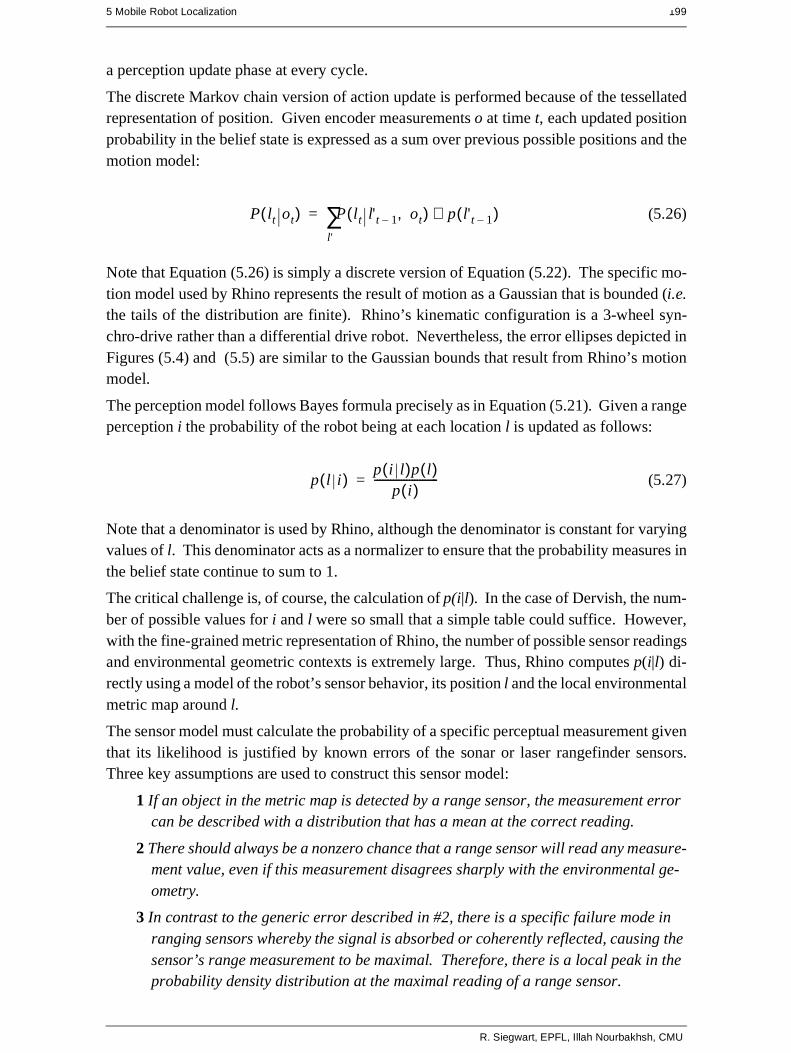
5 Mobile Robot Localization 199
a perception update phase at every cycle.
The discrete Markov chain version of action update is performed because of the tessellatedrepresentation of position. Given encoder measurements o at time t, each updated positionprobability in the belief state is expressed as a sum over previous possible positions and themotion model:
(5.26)
Note that Equation (5.26) is simply a discrete version of Equation (5.22). The specific mo-tion model used by Rhino represents the result of motion as a Gaussian that is bounded (i.e.the tails of the distribution are finite). Rhino’s kinematic configuration is a 3-wheel syn-chro-drive rather than a differential drive robot. Nevertheless, the error ellipses depicted inFigures (5.4) and (5.5) are similar to the Gaussian bounds that result from Rhino’s motionmodel.
The perception model follows Bayes formula precisely as in Equation (5.21). Given a rangeperception i the probability of the robot being at each location l is updated as follows:
(5.27)
Note that a denominator is used by Rhino, although the denominator is constant for varyingvalues of l. This denominator acts as a normalizer to ensure that the probability measures inthe belief state continue to sum to 1.
The critical challenge is, of course, the calculation of p(i|l). In the case of Dervish, the num-ber of possible values for i and l were so small that a simple table could suffice. However,with the fine-grained metric representation of Rhino, the number of possible sensor readingsand environmental geometric contexts is extremely large. Thus, Rhino computes p(i|l) di-rectly using a model of the robot’s sensor behavior, its position l and the local environmentalmetric map around l.
The sensor model must calculate the probability of a specific perceptual measurement giventhat its likelihood is justified by known errors of the sonar or laser rangefinder sensors.Three key assumptions are used to construct this sensor model:
1 If an object in the metric map is detected by a range sensor, the measurement errorcan be described with a distribution that has a mean at the correct reading.
2 There should always be a nonzero chance that a range sensor will read any measure-ment value, even if this measurement disagrees sharply with the environmental ge-ometry.
3 In contrast to the generic error described in #2, there is a specific failure mode inranging sensors whereby the signal is absorbed or coherently reflected, causing thesensor’s range measurement to be maximal. Therefore, there is a local peak in theprobability density distribution at the maximal reading of a range sensor.
P lt ot( ) P lt l't 1– ot,( ) p l't 1–( )⋅l'
∑=
p l i( )p i l( )p l( )
p i( )------------------------=
R. Siegwart, EPFL, Illah Nourbakhsh, CMU

200 Autonomous Mobile Robots
By validating these assumptions using empirical sonar trials in multiple environments, theresearch group has delivered to Rhino a conservative and powerful sensor model for its par-ticular sensors.
Figure 5.25 provides a simple 1D example of the grid-based Markov localization algorithm.The robot begins with a flat probability density function for its possible location. In otherwords, it initially has no bias regarding position. As the robot encounters first one door andthen a second door, the probability density function over possible positions becomes firstmultimodal and finally unimodal and sharply defined. The ability of a Markov localizationsystem to localize the robot from an initially lost belief state is its key distinguishing feature.
The resulting robot localization system has been part of a navigation system that has dem-onstrated great success both at the University of Bonn and at a public museum in Bonn. Thisis a challenging application because of the dynamic nature of the environment, as the robot’ssensors are frequently subject to occlusion due to humans gathering around the robot. Rhi-no’s ability to function well in this setting is a demonstration of the power of the Markovlocalization approach
Reducing computational complexity: Randomized Sampling
A great many steps are taken in real-world implementations such as Rhino in order to effectcomputational gains. These are valuable because, with an exact cell decomposition repre-sentation and use of raw sensor values rather than abstraction to features, such a robot has a
Fig 5.25 Improving belief state by moving. Roland, we need to re-make this picturefor copyright reasons probably.
5 Mobile Robot Localization 201
massive computational effort associated with each perceptual update.
One class of techniques deserves mention because it can significantly reduce the computa-tional overhead of techniques that employ fixed-cell decomposition representations. Thebasic idea, which we call randomized sampling is known alternatively as Particle filter al-gorithms, Condensation algorithms and Monte Carlo algorithms [ROLAND, reference theThrun et al. paper on "Robust Monte Carlo" in my text file].
Irrespective of the specific technique, the basic algorithm is the same in all these cases. In-stead of representing every possibe robot position by representing the complete and correctbelief state, an approximate belief state is constructed by representing only a subset of thecomplete set of possible locations that should be considered.
For example, consider a robot with a complete belief state of 10,000 possible locations attime t. Instead of tracking and updating all 10,000 possible locations based on a new sensormeasurement, the robot can select only 10% of the stored locations and update only thoselocations. By weighting this sampling process with the probability values of the locations,one can bias the system to generate more samples at local peaks in the probability densityfunction. So, the resulting 1,000 locations will be concentrated primarily at the highestprobability locations. This biasing is desirable, but only to a point.
We also wish to ensure that some less likely locations are tracked, as otherwise, if the robotdoes indeed receive unlikely sensor measurements, it will fail to localize. This randomiza-tion of the sampling process can be performed by adding additional samples from a flat dis-tribution for example. Further enhancements of these randomized methods enable thenumber of statistical samples to be varied on-the-fly, based for instance on the ongoing lo-calization confidence of the system. This further reduces the number of samples requiredon average while guaranteeing that a large number of samples will be used when necessary[ROLAND, reference the Fox NIPS article on KLD-Sampling Adaptive Particle Filters]
These sampling techniques have resulted in robots that function indistinguishably as com-pared to their full belief state set ancestors, yet use computationally a fraction of the resourc-es. Of course, such sampling has a penalty: completeness. The probabilistically completenature of Markov localization is violated by these sampling approaches because the robot isfailing to update all the nonzero probability locations, and thus there is a danger that the ro-bot, due to an unlikely but correct sensor reading, could become truly lost. Of course, re-covery from a lost state is feasible just as with all Markov localization techniques.
R. Siegwart, EPFL, Illah Nourbakhsh, CMU

202 Autonomous Mobile Robots
5.6.3 Kalman Filter Localization
The Markov localization model can represent any probability density function over robotposition. This approach is very general but, due to its generality, inefficient. A successfulalternative is to use a more compact representation of a specific class of probability densi-ties. The Kalman filter does just this, and is an optimal recursive data processing algorithm.It incorporates all information, regardless of precision, to estimate the current value of thevariable of interest. A comprehensive introduction can be found in [46] and a more detailedtreatment is presented in [28].
Figure 5.26 depicts the a general scheme of Kalman filter estimation, where the system hasa control signal and system error sources as inputs. A measuring device enables measuringsome system states with errors. The Kalman filter is a mathematical mechanism for produc-ing an optimal estimate of the system state based on the knowledge of the system and themeasuring device, the description of the system noise and measurement errors and the un-certainty in the dynamics models. Thus the Kalman filter fuses sensor signals and systemknowledge in an optimal way. Optimality depends on the criteria chosen to evaluate the per-formance and on the assumptions. Within the Kalman filter theory the system is assumed tobe linear and white with Gaussian noise. As we have discussed earlier, the assumption ofGaussian error is invalid for our mobile robot applications but, nevertheless, the results areextremely useful. In other engineering disciplines, the Gaussian error assumption has insome cases been shown to be quite accurate [46].
We begin with a subsection that introduces Kalman filter theory, then we present an appli-cation of that theory to the problem of mobile robot localization. Finally, the third subsec-tion will present a case study of a mobile robot that navigates indoor spaces by virtue ofKalman filter localization.
System
Fig 5.26 Typical Kalman filter application [46]
System state(desired butnot known)
Control
Measuringdevices
System errorsource
Measurementerror sources
Observedmeasurement
Optimal estimate ofsystem stateKalman
filter

5 Mobile Robot Localization 203
5.6.3.1 Introduction to Kalman Filter Theory
The basic Kalman filter method allows multiple measurements to be incorporated optimallyinto a single estimate of state. In demonstrating this, first we make the simplifying assump-tion that the state does not change (e.g. the robot does not move) between the acquisition ofthe first and second measurement. After presenting this static case, we can introduce dy-namic prediction readily.
Static Estimation
Assume we have taken two measurements, one with an ultrasonic range sensor at time k andone with a more precise laser range sensor at time k+1. Based on each measurement we areable to estimate the robot’s position. Such an estimate derived from the first sensor mea-surements is q1 and the estimate of position based on the second measurement is q2. Since
we know that each measurement can be inaccurate, we wish to modulate these position es-timates based on the measurement error expected from each sensor. Suppose that we use
two variances and to predict the error associated with each measurement. We will,
of course, assume a unimodal error distribution throughout the remainder of the Kalman fil-ter approach, yielding the two robot position estimates:
with variance (5.28)
with variance . (5.29)
So we have two measurements available to estimate the robots position. The question is,
how do we fuse (combine) these data to get the best estimate for the robot position?
We are assuming that there was no robot motion between time k and time k+1, and thereforewe can directly apply the same weighted least square technique of Equation 4.61 in Section4.3.1.1. Thus we write:
(5.30)
with wi being the weight of measurement i. To find the minimum error we set the derivative
of S equal to zero.
(5.31)
σ12 σ2
2
q1 q1= σ12
q2 q2= σ22
q
S wi q qi–( )2
i 1=
n
∑=
S∂q∂
-----q∂∂
wi q qi–( )2
i 1=
n
∑ 2 wi q qi–( )i 1=
n
∑ 0= = =
R. Siegwart, EPFL, Illah Nourbakhsh, CMU

204 Autonomous Mobile Robots
(5.32)
(5.33)
If we take as the weight wi
(5.34)
then the value of in terms of two measurements can be defined as follows:
(5.35)
; (5.36)
Note that, from (5.36) we can see that the resulting variance is less than all the variances
of the individual measurements. Thus the uncertainty of the position estimate has been
decreased by combining the two measurements. This demonstrates that even poor measure-ments only increase the precision of an estimate (fig. 5.27), a result that we expect based onInformation Theory.
Equation (5.35) can be rewritten as
(5.37)
or, in final form that is used in Kalman filter implementation
wiq
i 1=
n
∑ wiqi
i 1=
n
∑– 0=
q
wiqi
i 1=
n
∑
wi
i 1=
n
∑-------------------=
wi1
σi2
-----=
q
q
1
σ12
-----q11
σ22
-----q2+
1
σ12
----- 1
σ22
-----+----------------------------
σ22
σ12 σ2
2+
----------------q1
σ12
σ12 σ2
2+
----------------q2+= =
1
σ2----- 1
σ12
----- 1
σ22
-----+σ2
2 σ12
+
σ12σ2
2----------------= = σ2
σ12σ2
2
σ22 σ1
2+
----------------=
σ2
σi2
q q1
σ12
σ12 σ2
2+
---------------- q2 q– 1( )+=

5 Mobile Robot Localization 205
(5.38)
where
; ; (5.39)
Equation (5.38) tells us, that the best estimate of the state at time k+1 is equal
to the best prediction of the value before the new measurement is taken, plus a cor-
rection term of an optimal weighting value times the difference between and the best
prediction at time k+1. The updated variance of the state is given using equation
(5.36)
(5.40)
Dynamic Estimation
Next, consider a robot that moves between successive sensor measurements. Suppose thatthe motion of the robot between times k and k+1 is described by the velocity u and the noisew which represents the uncertainty of the actual velocity:
(5.41)
Fig 5.27 Fusing probability density of two estimates [46]
xk 1+ xk Kk 1+ zk 1+ xk–( )+=
Kk 1+
σk2
σk2 σz
2+
----------------= σk2 σ1
2= σz
2 σ22
=
xk 1+ xk 1+
xk zk 1+
zk 1+
xk 1+ xk 1+
σk 1+2 σk
2Kk 1+ σk
2–=
dxdt------ u w+=
R. Siegwart, EPFL, Illah Nourbakhsh, CMU

206 Autonomous Mobile Robots
If we now start at time k, knowing the variance of the robot position at this time and
knowing the variance of the motion, we obtain for the time just when the measure-
ment is taken:
(5.42)
(5.43)
where:
tk’ = tk+1
tk+1 and tk are the time in seconds at k+1 and k respectively.
Thus is the optimal prediction of the robot’s position just as the measurement is taken
at time k+1. It describes the growth of position error until a new measurement is taken (fig.5.28).
We can now rewrite equation (5.38) and (5.39) using equation (5.42) and (5.43).
(5.44)
(5.45)
The optimal estimate at time k+1 is given by the last estimate at k and the estimate of therobot motion including the estimated movement errors.
By extending the above equations to the vector case and allowing time varying parametersin the system and a description of noise, we can derive the Kalman filter localization algo-rithm.
σk2
σw2
k′
xk′ xk u tk 1+ tk–( )+=
σk′2 σk
2 σw2
tk 1+ tk–[ ]+=
xk ′
Fig 5.28 Propagation of probability density of a moving robot [46]
k 1+ xk′ Kk 1+ zk 1+ xk ′–( )+=
xk 1+ xk u tk 1+ tk–( )+[ ] Kk 1+ zk 1+ xk– u tk 1+ tk–( )–[ ]+=
Kk 1+
σk ′2
σk ′2 σz
2+
-------------------σk
2 σw2
tk 1+ tk–[ ]+
σk2 σw
2tk 1+ tk–[ ] σz
2+ +
------------------------------------------------------= =

5 Mobile Robot Localization 207
5.6.3.2 Application to mobile robots: Kalman filter localization
The Kalman filter is an optimal and efficient sensor fusion technique. Application of theKalman filter to localization requires posing the robot localization problem as a sensor fu-sion problem. Recall that the basic probabilistic update of robot belief state can be segment-ed into two phases, perception update and action update as specified by Equations 5.21 and5.22.
The key difference between the Kalman filter approach and our earlier Markov localizationapproach lies in the perception update process. In Markov localization, the entire percep-tion, i.e. the robot’s set of instantaneous sensor measurements, is used to update each possi-ble robot position in the belief state individually using Bayes formula. In some cases, theperception is abstract, having been produced by a feature extraction mechanism as in Der-vish. In other cases, as with Rhino, the perception consists of raw sensor readings.
By contrast, perception update using a Kalman filter is a multi-step process. The robot’s to-tal sensory input is treated, not as a monolithic whole, but as a set of extracted features thateach relate to objects in the environment. Given a set of possible features, the Kalman filteris used to fuse the distance estimate from each feature to a matching object in the map. In-stead of carrying out this matching process for many possible robot locations individuallyas in the Markov approach, the Kalman filter accomplishes the same probabilistic update bytreating the whole, unimodal and Gaussian belief state at once. Figure 5.29 depicts the par-ticular schematic for Kalman filter localization.
The first step is action update or position prediction, the straightforward application of aGaussian error motion model to the robot’s measured encoder travel. The robot then collectsactual sensor data and extracts appropriate features (e.g. lines, doors, or even the value of aspecific sensor) in the observation step. At the same time, based on its predicted position inthe map, the robot generates a measurement prediction which identifies the features that the
Actual Observationson-board sensors
Mapdata base
Position PredictionObservation Prediction
Fig 5.29 Schematic for Kalman filter mobile robot localization (see [9])
Per
cept
ion
Matching
Estimation(fusion)
raw sensor data or ex-tracted features
pred
icte
dob
serv
a-tio
ns
positionestimate
matched predictionsand actual observations
YES
Encoder
R. Siegwart, EPFL, Illah Nourbakhsh, CMU
208 Autonomous Mobile Robots
robot expects to find and the positions of those features. In matching the robot identifies thebest pairings between the features actually extracted during observation and the expectedfeatures due to measurement prediction. Finally, the Kalman filter can fuse the informationprovided by all of these matches in order to update the robot belief state in estimation.
In the following sub-sections these five steps are described in greater detail. The presenta-tion is based on the work of Leonard and Durrant-Whyte [9 page 61-65].
1. Robot Position Prediction
The robot’s position at time step k+1 is predicted based on its old location (at time step k)
and its movement due to the control input :
(5.46)
For the differential drive robot, is derived in Equations (5.6) and (5.7) re-
spectively.
Knowing the plant and error model, we can also compute the variance associ-
ated with this prediction (see eq. (5.9) section 5.2.4):
(5.47)
This allows us to predict the robot’s position and its uncertainty after a movement specified
by the control input . Note that the belief state is assumed to be Gaussian, and so we
can characterize the believe state with just the two parameters and .
2. Observation
The second step it to obtain sensor measurements from the robot at time k+1. In
this presentation, we assume that the observation is the result of a feature extraction process
executed on the raw sensor data. Therefore, the observation consists of a set of single
observations extracted from various sensors. Formally each single observation can
represent an extracted features such as a line or door, or even a single, raw sensor value.
The parameters of the features are usually specified in the sensor frame and therefore in alocal reference frame of the robot. However, for matching we need to represent the obser-
vations and measurement predictions in the same frame . In our presentation we will
transform the measurement predictions from the global coordinate frame to the sensor frame
. This transformation is specified in the function discussed in the next paragraph.
u k( )
p k 1 k+( ) f p k k( ) u k( ),( )=
p k 1 k+( ) p'=
Σp k 1 k+( )
Σp k 1 k+( ) ∇ pf Σp k k( ) ∇ pfT ∇ uf Σu k( ) ∇ uf
T⋅⋅+⋅⋅=
u k( )p k 1 k+( ) Σp k 1 k+( )
Z k 1+( )
n0
zj k 1+( )
S{ }
S{ } hi
5 Mobile Robot Localization 209
3. Measurement Prediction
We use the predicted robot position and the map to generate multiple pre-
dicted feature observations . Each predicted feature has its position transformed into the
sensor frame:
(5.48)
We can define the measurement prediction as the set containing all predicted feature ob-
servations:
(5.49)
The predicted state estimate is used to compute the measurement Jacobian
for each prediction. As you will see in the example below, the function is mainly a coor-
dinate transformation between the world frame and the sensor frame.
4. Matching
At this point we have a set of actual, single observations, which are features in sensor space,and we also have a set of predicted features, also positioned in sensor space. The matchingstep has the purpose of identifying all of the single observations that match specific predict-ed features well enough to be used during the estimation process. In other words, we will,for a subset of the observations and a subset of the predicted features, find pairings that in-tuitively say "this observation is the robot’s measurement of this predicted feature based onthe map."
Formally, the goal of the matching procedure is to produce an assignment from observations
to the targets (stored in the map). For each measurement prediction for which
a corresponding observation is found we calculate the innovation . Innovation is
a measure of the difference between the predicted and observed measurements:
(5.50)
The innovation covariance can be found by applying the error propagation
law (section 4.2.3 equation (4.60)):
(5.51)
where represents the covariance (noise) of the measurement .
To determine the validity of the correspondence between measurement prediction and ob-servation, a validation gate has to be specified. A possible definition of the validation gateis the Mahalanobis distance:
p k 1 k+( ) M k( )
zt
ziˆ k 1+( ) hi zt p k 1+ k( ),( )=
nt
Z k 1+( ) ziˆ k 1+( ) 1 i nt≤ ≤( ){ }=
p k 1 k+( ) ∇ hi
hi
zj k 1+( ) zt
vij k 1+( )
vij k 1+( ) zj k 1+( ) zi k 1+( )–[ ]=vij k 1+( ) zj k 1+( ) hi zt p k 1+ k( ),( )–[ ]=
ΣIN ij, k 1+( )
ΣIN ij, k 1+( ) ∇ hi Σp k 1+ k( ) ∇ hiT ΣR i, k 1+( )+⋅⋅=
ΣR i, k 1+( ) zi k 1+( )
R. Siegwart, EPFL, Illah Nourbakhsh, CMU

210 Autonomous Mobile Robots
(5.52)
However, dependent on the application, the sensors and the environment models, more so-phisticated validation gates might be employed.
The validation equation is used to test observation for membership in the valida-
tion gate for each predicted measurement. When a single observation falls in the validationgate, we get a successful match. If one observation falls in multiple validation gates, the bestmatching candidate is selected or multiple hypothesis are tracked. Observations that do notfall in the validation gate are simply ignored for localization. Such observations could haveresulted from objects not in the map, such as new objects (e.g. someone places a large boxin the hallway) or transient objects (e.g. humans standing next to the robot may form a linefeature). One approach is to take advantage of such unmatched observations to populate therobot’s map.
5. Estimation: applying the Kalman Filter
Next we compute the best estimate of the robot’s position based on the po-
sition prediction and all the observations at time k+1. To do this position update, we first
stack the validated observations into a single vector to form and desig-
nate the composite innovation . Then we stack the measurement Jacobians for
each validated measurement together to form the composite Jacobian and the measure-
ment error (noise) vector . We can then compute the com-
posite innovation covariance according to equation (5.51) and by utilizing the
well-known result [28] that the Kalman gain can be written as
(5.53)
we can update the robot’s position estimate
(5.54)
with the associated variance
(5.55)
For the one-dimensional case and with we can show that this for-
mula corresponds to the 1D case derived earlier:
Equation 5.53 is simplified to:
vijT
k 1+( ) ΣIN ij,1–
k 1+( ) vij k 1+( ) g2≤⋅⋅
zj k 1+( )
p k 1 k 1+ +( )
zj k 1+( ) z k 1+( )
v k 1+( ) hi∇
h∇ΣR k 1+( ) diag ΣR i, k 1+( )[ ]=
ΣIN k 1+( )
K k 1+( ) Σp k 1 k+( ) hT ΣIN
1–k 1+( )⋅∇⋅=
p k 1 k 1+ +( ) p k 1 k+( ) K k 1+( ) v k 1+( )⋅+=
Σp k 1 k 1+ +( ) Σp k 1 k+( ) K– k 1+( ) ΣIN k 1+( ) KT
k 1+( )⋅⋅=
hi zt p k 1+ k( ),( ) zt=
5 Mobile Robot Localization 211
(5.56)
corresponding to equation (5.45) and Equation 5.54 simplifies to:
(5.57)
corresponding to equation (5.44).
5.6.3.3 Case study: Kalman filter localization with line feature extraction
The Pygmalion robot at EPFL is a differential drive robot that uses a laser rangefinder as itsprimary sensor [39], [76]. In contrast to both Dervish and Rhino, the environmental repre-sentation of Pygmalion is continuous and abstract: the map consists of a set of infinite linesdescribing the environment. Pygmalion’s belief state is, of course, represented as a Gauss-ian distribution since this robot uses the Kalman filter localization algorithm. The value of
its mean position is represented to a high level of precision, enabling Pygmalion to local-
ize with very high precision when desired. Below, we present details for Pygmalion’s im-plementation of the five Kalman filter localization steps. For simplicity we assume that the
sensor frame is equal to the robot frame . If not specified all the vectors are rep-
resented in the world coordinate system .
1. Robot Position Prediction
At the time increment k the robot is at position and its best po-
sition estimate is . The control input drives the robot to the position
(fig. 5.30).
The robot position prediction at the time increment k+1 can be computed from the
previous estimate and the odometric integration of the movement. For the differen-
tial drive that Pygmalion has we can use the model (odometry) developed in section 5.2.4:
K k 1+( )σp
2k 1 k+( )
σIN2
k 1+( )---------------------------
σp2
k 1 k+( )
σp2
k 1+ k( ) σR2
k 1+( )+--------------------------------------------------------= =
k 1 k 1+ +( ) p k 1 k+( ) K k 1+( ) v k 1+( )⋅+=
k 1 k 1+ +( ) p k 1 k+( ) K k 1+( ) zj k 1+( ) hi zt p k 1+ k( ),( )–[ ]⋅+=
p k 1 k 1+ +( ) p k 1 k+( ) K k 1+( ) zj k 1+( ) zt–[ ]⋅+=
µ
S{ } R{ }W{ }
p k( ) x k( ) y k( ) θ k( )T
=
p k k( ) u k( ) p k 1+( )
p k 1+( )
p k k( )
R. Siegwart, EPFL, Illah Nourbakhsh, CMU
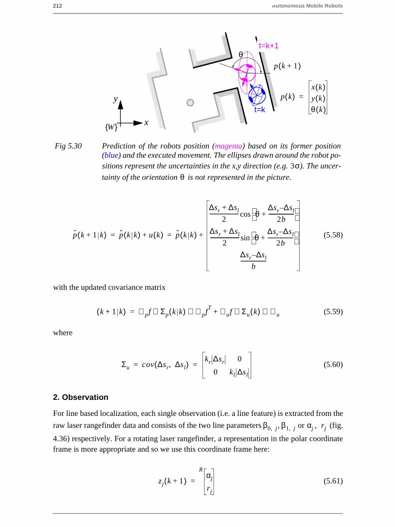
212 Autonomous Mobile Robots
(5.58)
with the updated covariance matrix
(5.59)
where
(5.60)
2. Observation
For line based localization, each single observation (i.e. a line feature) is extracted from the
raw laser rangefinder data and consists of the two line parameters , or , (fig.
4.36) respectively. For a rotating laser rangefinder, a representation in the polar coordinateframe is more appropriate and so we use this coordinate frame here:
(5.61)
x
y
Fig 5.30 Prediction of the robots position (magenta) based on its former position(blue) and the executed movement. The ellipses drawn around the robot po-sitions represent the uncertainties in the x,y direction (e.g. ). The uncer-
tainty of the orientation is not represented in the picture.
3σθ
t=k
t=k+1
p k( )x k( )y k( )θ k( )
=
p k 1+( )θ
W{ }
p k 1 k+( ) p k k( ) u k( )+ p k k( )
∆sr ∆sl+
2---------------------- θ
∆sr ∆– sl
2b-------------------+
cos
∆sr ∆sl+
2---------------------- θ
∆sr ∆– sl
2b-------------------+
sin
∆sr ∆– sl
b-------------------
+= =
k 1 k+( ) ∇ pf Σp k k( ) ∇ pfT ∇ uf Σu k( ) ∇ u⋅⋅+⋅⋅=
Σu cov ∆sr ∆sl,( )kr ∆sr 0
0 kl ∆sl
= =
β0 j, β1 j, αj rj
zj k 1+( )αj
rj
R
=

5 Mobile Robot Localization 213
After acquiring the raw data at time k+1, lines and their uncertainties are extracted (fig.
5.31a/b). This leads to observed lines with line parameters (5.31c) and a covari-
ance matrix for each line that can be calculated from the uncertainties of all the measurementpoints contributing to each line as developed for line extraction in Section 4.3.1.1:
(5.62)
3. Measurement Prediction
Base on the stored map and the predicted robot position , the measurement predic-
tions of expected features are generated (fig. 5.32). To reduce the required calculation
power, there is often an additional step that first selects the possible features, in this caselines, from the whole set of features in the map. These lines are stored in the map and spec-
ified in the world coordinate system . Therefore they need to be transformed to the ro-
bot frame :
Fig 5.31 Observation: From the raw data(a) acquired by the laser scannerat time k+1, lines are extracted(b). The line parameters and
and its uncertainties can be
represented in the model space(c).
αj
rj
−5 −4 −3 −2 −1 0 1 2 3 4−5
−4
−3
−2
−1
0
1
2
3
4
5
x [m]
y [m
]
−5 −4 −3 −2 −1 0 1 2 3 4−5
−4
−3
−2
−1
0
1
2
3
4
5
x [m]
y [m
]
αj
rj
line j
a b
αj
r
π-π
line j
0
rj
c
n0 2n0
ΣR j,σαα σαr
σrα σrr j
=
p k k( )
t i,
W{ }R{ }
R. Siegwart, EPFL, Illah Nourbakhsh, CMU
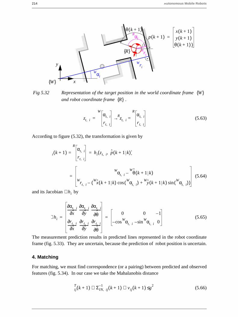
214 Autonomous Mobile Robots
(5.63)
According to figure (5.32), the transformation is given by
(5.64)
and its Jacobian by
(5.65)
The measurement prediction results in predicted lines represented in the robot coordinateframe (fig. 5.33). They are uncertain, because the prediction of robot position is uncertain.
4. Matching
For matching, we must find correspondence (or a pairing) between predicted and observedfeatures (fig. 5.34). In our case we take the Mahalanobis distance
(5.66)
x
y
Fig 5.32 Representation of the target position in the world coordinate frame
and robot coordinate frame .
W{ }R{ }
R{ }
p k 1+( )x k 1+( )y k 1+( )θ k 1+( ) )
=αR i
rR
i
θ k 1+( )
rW
i
W{ }αW
i
zt i,αt i,
rt i,
W
zR
t i,αt i,
rt i,
R
=→=
i k 1+( )αt i,
rt i,
R
= hi zt i, p k 1+ k( ),( )=
i k 1+( )αW
t i, θ k 1 k+( )W
–
rW
t i, x k 1 k+( )W αWt i,( )cos y k 1 k+( )W αW
t i,( )sin+( )–=
hi∇
hi∇
αt i,∂x∂
------------αt i,∂
y∂------------
αt i,∂
θ∂------------
rt i,∂x∂
-----------rt i,∂y∂
-----------rt i,∂
θ∂-----------
0 0 1–
αWt i,cos– αW
t i,sin– 0= =
ijT
k 1+( ) ΣIN ij,1–
k 1+( ) vij k 1+( ) g2≤⋅⋅

5 Mobile Robot Localization 215
with
(5.67)
(5.68)
to enable finding the best matches while eliminating all other remaining observed and pre-
Fig 5.33 Measurement predictions:Based on the map and theestimated robot position thetargets (visible lines) arepredicted. They are repre-sented in the model spacesimilar to the observations. αi
r
π-π
line i
0
ri
Fig 5.34 Matching: The observations (green) and measurement prediction (magen-ta) are matched and the innovation and its uncertainties are calculated.
αi
r
π-π
match j,i
0
ri
αj
rj
No match!!Wall was not
observed.
image space model space
vij k 1+( ) zj k 1+( ) hi zt p k 1+ k( ),( )–[ ]=
vij k 1–( )αj
rj
αWt i, θ k 1 k+( )
W–
rW
t i, x k 1 k+( )W αWt i,( )cos y k 1 k+( )W αW
t i,( )sin+( )––=
ΣIN ij, k 1+( ) ∇ hi Σp k 1+ k( ) ∇ hiT ΣR i, k 1+( )+⋅⋅=
R. Siegwart, EPFL, Illah Nourbakhsh, CMU

216 Autonomous Mobile Robots
dicted unmatched features.
5. Estimation
Applying the Kalman filter results in a final pose estimate corresponding to the weightedsum of (fig 5.35)
– the pose estimates of each matched pairing of observed and predicted features
– robot position estimation based on odometry and observation positions
Fig 5.35 Kalman filter estimation of the new robot position: By fusing the predictionof robot position (magenta) with the innovation gained by the measurements
(green) we get the updated estimate of the robot position (red).p k k( )

5 Mobile Robot Localization 217
5.7 Other Examples of Localization Systems
Markov localization and Kalman filter localization have been two extremely popular strat-egies for research mobile robot systems navigating indoor environments. They have strongformal bases and therefore well-defined behavior. But there are a large number of other lo-calization techniques that have been used with varying degrees of success on commercialand research mobile robot platforms. We will not explore the space of all localization sys-tems in detail. Refer to surveys such as [4] for such information.
There are, however, several categories of localization techniques that deserve mention. Notsurprisingly, many implementations of these techniques in commercial robotics employmodifications of the robot’s environment, something that the Markov localization and Kal-man filter localization communities eschew. In the following sections, we briefly identifythe general strategy incorporated by each category and reference example systems, includ-ing as appropriate those that modify the environment and those that function without envi-ronmental modification.
Landmark-based navigation
Landmarks are generally defined as passive objects in the environment that provide a highdegree of localization accuracy when they are within the robot’s field of view. Mobile ro-bots that make use of landmarks for localization generally use artificial markers that havebeen placed by the robot’s designers to make localization easy.
The control system for a landmark-based navigator consists of two discrete phases. Whena landmark is in view, the robot localizes frequently and accurately, using action update andperception update to track its position without cumulative error. But when the robot is in nolandmark "zone," then only action update occurs, and the robot accumulates position uncer-tainty until the next landmark enters the robot’s field of view.
The robot is thus effectively dead-reckoning from landmark zone to landmark zone. This inturn means the robot must consult its map carefully, ensuring that each motion betweenlandmarks is sufficiently short, given its motion model, that it will be able to localize suc-cessful upon reaching the next landmark.
Figure 5.36 shows one instantiation of landmark-based localization. The particular shape ofthe landmarks enables reliable and accurate pose estimation by the robot, which must travel
Fig 5.36 Z-shaped landmarks on the ground
R. Siegwart, EPFL, Illah Nourbakhsh, CMU

218 Autonomous Mobile Robots
using dead reckoning between the landmarks.
One key advantage of the landmark-based navigation approach is that a strong formal theoryhas been developed for this general system architecture [113]. In this work, the authors haveshown precise assumptions and conditions which, when satisfied, guarantee that the robotwill always be able to localize successfully. This work also led to a real-world demonstra-tion of landmark-based localization. Standard sheets of paper were placed on the ceiling ofthe Robotics Laboratory at Stanford University, each with a unique checkerboard pattern.A Nomadics 200 mobile robot was fitted with a monochrome CCD camera aimed verticallyup at the ceiling. By recognizing the paper landmarks, which were placed approximately 2meters apart, the robot was able to localize to within several centimeters, then move usingdead-reckoning to another landmark zone.
The primary disadvantage of landmark-based navigation is that in general it requires signif-icant environmental modification. Landmarks are local, and therefore a large number is usu-ally required to cover a large factory area or research laboratory. For example, the RoboticsLaboratory at Stanford made use of approximately 30 discrete landmarks, all affixed indi-vidually to the ceiling.
Globally unique localization
The landmark-based navigation approach makes a strong general assumption: when thelandmark is in the robot’s field of view, localization is essentially perfect. One way to reachthe Holy Grail of mobile robotic localization is to effectively enable such an assumption tobe valid no matter where the robot is located. It would be revolutionary if a look at the ro-bot’s sensors immediately identified its particular location, uniquely, and repeatedly.
Such a strategy for localization is surely aggressive, but the question of whether it can bedone is primarily a question of sensor technology and sensing software. Clearly, such a lo-calization system would need to use a sensor that collects a very large amount of informa-tion. Since vision does indeed collect far more information than previous sensors, it hasbeen used as the sensor of choice in research towards globally unique localization.
Figure (4.50) depicts the image taken by a catadioptric camera system. If humans were ableto look at an individual such picture and identify the robot’s location in a well-known envi-ronment, then one could argue that the information for globally unique localization does ex-ist within the picture; it must simply be teased out.
One such approach has been attempted by several researchers and involves constructing oneor more image histograms to represent the information content of an image stably (see forexample Figure 4.51 and Section 4.3.2.2). A robot using such an image histogramming sys-tem has been shown to uniquely identify individual rooms in an office building as well asindividual sidewalks in an outdoor environment. However, such a system is highly sensitiveto external illumination and provides only a level of localization resolution equal to the vi-sual footprint of the camera optics.
The Angular histogram depicted in Figure 5.37 is another example in which the robot’s sen-sor values are transformed into an identifier of location. However, due to the limited infor-

5 Mobile Robot Localization 219
mation content of sonar ranging strikes, it is likely that two places in the robot’s environmentmay have angular histograms that are too similar to be differentiated successfully.
One way of attempting to gather sufficient sonar information for global localization is to al-low the robot time to gather a large amount of sonar data into a local evidence grid (i.e. oc-cupancy grid) first, then match the local evidence grid with a global metric map of theenvironment. In [115] the researchers demonstrate such a system as able to localize on-the-fly even as significant changes are made to the environment, degrading the fidelity of themap. Most interesting is that the local evidence grid represents information well enough thatit can be used to correct and update the map over time, thereby leading to a localization sys-tem that provides corrective feedback to the environment representation directly. This issimilar in spirit to the idea of taking rejected observed features in the Kalman filter localiza-tion algorithm and using them to create new features in the map.
A most promising, new method for globally unique localization is called Mosaic-based lo-calization [114]. This fascinating approach takes advantage of an environmental feature thatis rarely used by mobile robots: fine-grained floor texture. This method succeeds primarilybecause of the recent ubiquity of very fast processors, very fast cameras and very large stor-age media.
The robot is fitted with a high-quality high-speed CCD camera pointed toward the floor, ide-ally situated between the robot’s wheels and illuminated by a specialized light pattern offthe camera axis to enhance floor texture. The robot begins by collecting images of the entirefloor in the robot’s workspace using this camera. Of course the memory requirements aresignificant, requiring a 10GB drive in order to store the complete image library of a 300 x300 meter area.
Once the complete image mosaic is stored, the robot can travel any trajectory on the floorwhile tracking its own position without difficulty. Localization is performed by simply re-
Fig 5.37 The angular histogram: Example
R. Siegwart, EPFL, Illah Nourbakhsh, CMU

220 Autonomous Mobile Robots
cording one image, performing action update, then performing perception update by match-ing the image to the mosaic database using simple techniques based on image databasematching. The resulting performance has been impressive: such a robot has been shown tolocalize repeatedly with 1mm precision while moving at 25 km/hr.
The key advantage of globally unique localization is that, when these systems function cor-rectly, they greatly simplify robot navigation. The robot can move to any point and will al-ways be assured of localizing by collecting a sensor scan.
But the main disadvantage of globally unique localization is that it is likely that this methodwill never offer a complete solution to the localization problem. There will always be caseswhere local sensory information is truly ambiguous and, therefore, globally unique localiza-tion using only current sensor information is unlikely to succeed. Humans often have excel-lent local positioning systems, particularly in non-repeating and well-known environmentssuch as their homes. However, there are a number of environments in which such immediatelocalization is challenging even for humans: consider hedge mazes and large new officebuildings with repeating halls that are identical. Indeed, the mosaic-based localization pro-totype described above encountered such a problem in its first implementation. The floor ofthe factory floor had been freshly painted and was thus devoid of sufficient micro-fracturesto generate texture for correlation. Their solution was to modify the environment after all,painting random texture onto the factory floor.
Positioning Beacon systems
One of the most reliable solutions to the localization problem is to design and deploy an ac-tive beacon system specifically for the target environment. This is the preferred techniqueused by both industry and military applications as a way of ensuring the highest possible re-liablility of localization. The GPS system can be considered as just such a system (see Sec-tion 4.1.5.1).
Figure 5.38 depicts one such beacon arrangement for a collection of robots. Just as withGPS, by designing a system whereby the robots localize passively while the beacons are ac-tive, any number of robots can simultaneously take advantage of a single beacon system. As
Fig 5.38 Active ultrasonic beacons.

5 Mobile Robot Localization 221
with most beacon systems, the design depicted depends foremost upon geometric principlesto effect localization. In this case the robots must know the positions of the two pinger unitsin the global coordinate frame in order to localize themselves to the global coordinate frame.
A popular type of beacon system in industrial robotic applications is depicted in Figure 5.39.In this case beacons are retroreflective markers that can be easily detected by a mobile robotbased on their reflection of energy back to the robot. Given known positions for the opticalretroreflectors, a mobile robot can identify its position whenever it has three such beaconsin sight simultaneously. Of course, a robot with encoders can localize over time as well, anddoes not need to measure its angle to all three beacons at the same instant.
The advantage of such beacon-based systems is usually extremely high engineered reliabil-ity. By the same token, significant engineering usually surrounds the installation of such asystem in a specific commercial setting. Therefore, moving the robot to a different factoryfloor will be both time-consuming and expensive. Usually, even changing the routes usedby the robot will require serious re-engineering.
Route-based localization
Even more reliable than beacon-based systems are route-based localization strategies. Inthis case, the route of the robot is explicitly marked so that it can determine its position, notrelative to some global coordinate frame, but relative to the specific path it is allowed to trav-el. There are many techniques for marking such a route and the subsequent intersections.In all cases, one is effectively creating a railway system, except that the railway system issomewhat more flexible and certainly more human-friendly than a physical rail. For exam-ple, high uv-reflective, optically transparent paint can mark the route such that only the ro-bot, using a specialized sensor, easily detects it. Alternatively, a guide wire buriedunderneath the hall can be detected using inductive coils located on the robot chassis.
In all such cases, the robot localization problem is effectively trivialized by forcing the robotto always follow a prescribed path. To be fair, there are new industrial unmanned guided
Fig 5.39 Passive optical beacons
R. Siegwart, EPFL, Illah Nourbakhsh, CMU

222 Autonomous Mobile Robots
vehicles that do deviate briefly from their route in order to avoid obstacles. Nevertheless,the cost of this extreme reliability is obvious: the robot is much more inflexible give suchlocalization means, and therefore any change to the robot’s behavior requires significant en-gineering and time.

5 Mobile Robot Localization 223
5.8 Autonomous Map Building
All of the localization strategies we have discussed require human effort to install the robotinto a space. Artificial environmental modifications may be necessary. Even if this is notso, a map of the environment must be created for the robot. But a robot that localizes suc-cessfully has the right sensors for detecting the environment, and so the robot ought to buildits own map. This ambition goes to the heart of autonomous mobile robotics. In prose, wecan express our eventual goal as follows:
Starting from an arbitrary initial point, a mobile robot should be able to autonomously ex-plore the environment with its on board sensors, gain knowledge about it, interpret thescene, build an appropriate map and localize itself relative to this map.
Accomplishing this goal robustly is probably years away, but an important subgoal is theinvention of techniques for autonomous creation and modification of an environment map.Of course a mobile robot’s sensors have only limited range, and so it must physically exploreits environment to build such a map. So, the robot must not only create a map but it must doso while moving and localizing to explore the environment. In the robotics community, thisis often called the Simultaneous Localization and Mapping (SLAM) problem, arguably themost difficult problem specific to mobile robot systems.
The reason that SLAM is difficult is born precisely from the interaction between the robot’sposition updates as it localizes and its mapping actions. If a mobile robot updates its positionbased on an observation of an imprecisely known feature, the resulting position estimate be-comes correlated with the feature location estimate. Similarly, the map becomes correlatedwith the position estimate if an observation taken from an imprecisely known position isused to update or add a feature to the map. The general problem of map building is thus anexample of a chicken-and-egg problem. For localization the robot needs to know where thefeatures are whereas for map building the robot needs to know where it is on the map.
The only path to a complete and optimal solution to this joint problem is to consider all thecorrelations between between position estimation and feature location estimation. Suchcross-correlated maps are called stochastic maps, and we begin with a discussion of the the-ory behind this approach in the following sub-section [75].
Unfortunately, implementing such an optimal solution is computationally prohibitive. In re-sponse a number of researchers have offered other solutions that have functioned well inlimited circumstances. Section (5.8.2) characterizes these alternative partial solutions.
5.8.1 The Stochastic Map technique
Figure 5.40 shows a general schematic incorporating map building and maintenance into thestandard localization loop depicted by Figure (5.29) during discussion of Kalman filter lo-calization [9]. The added arcs represent the additional flow of information that occurs whenthere is an imperfect match between observations and measurement predictions.
Unexpected observations will affect the creation of new features in the map whereas unob-served measurement predictions will affect the removal of features from the map. As dis-cussed earlier, each specific prediction or observation has an unknown exact value and so it
R. Siegwart, EPFL, Illah Nourbakhsh, CMU

224 Autonomous Mobile Robots
is represented by a distribution. The uncertainties of all of these quantities must be consid-ered throughout this process.
The new type of map we are creating not only has features in it as did previous maps, but italso has varying degrees of probability that each feature is indeed part of the environment.
We represent this new map M with a set n of probabilistic feature locations , each with the
covariance matrix and an associated credibility factor between 0 and 1 quantifying the
belief in the existence of the feature in the environment (see Fig. (5.41)):
(5.69)
In contrast to the map used for Kalman filter localization previously, the map M is not as-sumed to be precisely known because it will be created by an uncertain robot over time. This
is why the features are described with associated covariance matrices .
Observationon-board sensors
Prediction ofMeasurement andPosition (odometry)
Fig 5.40 General schematic for concurrent localization and map building (see [9])
Per
cept
ion
Matching
Estimation(fusion)using confirmed map
raw sensor data orextracted features
pre
dict
edfe
atur
eob
serv
atio
ns
positionestimate
matched predictionsand observations
YES
Encoder
Map
Refine FeatureParameters
increase credibility
Add NewFeatures
extend map
Remove OffensiveFeatures
decrease credibility
Map Building and Maintenance
UnexpectedObservation?
YES
unexpectedobservations
NO NO
unobservedpredictions
zt
Σt ct
M zt Σt ct 1 t n≤ ≤( ), ,{ }=
zt Σt

5 Mobile Robot Localization 225
Just as with Kalman filter localization, the matching step yields has three outcomes in regardto measurement predictions and observations: matched prediction and observations, unex-pected observations and unobserved predictions. Localization, or the position update of therobot, proceeds as before. However, the map is also updated now, using all three outcomesand complete propagation of all the correllated uncertainties (see [9] for more details).
An interesting variable is the credibility factor , which governs the likelihood that the
mapped feature is indeed in the environment. How should the robot’s failure to match ob-served features to a particular map feature reduce that map feature’s credibility? And also,how should the robot’s success at matching a mapped feature increase the chance that themapped feature is "correct?" In [9] the following function is proposed for calculating cred-ibility:
(5.70)
where a and b define the learning and forgetting rate and ns and nu are the number of
matched and unobserved predictions up to time k, respectively. The update of the covari-
ance matrix can be done similarly to the position update seen in previous section. In map-
building the feature positions and the robot’s position are strongly correlated. This forcesus to use a stochastic map, in which all cross-correlations must be updated in each cycle [73,74, 75].
The stochastic map consists of a stacked system state vector:
(5.71)
and a system state covariance matrix:
Cαr
σα2 σαr
σαr σr2
=
x1
y1
x0
y0
Fig 5.41 Uncertainties in the map.
Extracted line
Map feature
Updatedfeature
α
r
rW{ } αW{ }
rS{ } αS{ }
ct
ct k( ) 1 e
ns
a----
nu
b-----–
–
–=
Σt
X xr k( ) x1 k( ) x2 k( ) …xn k( )T
=
R. Siegwart, EPFL, Illah Nourbakhsh, CMU

226 Autonomous Mobile Robots
(5.72)
where the index r stands for the robot and the index i = 1 to n for the features in the map.
In contrast to localization based on an a priori accurate map, in the case of a stochastic mapthe cross-correlations must be maintained and updated as the robot is performing automaticmap-building. During each localization cycle, the cross-correlations robot-to-feature andfeature-to-robot are also updated. In short, this optimal approach requires every value in themap to depend on every other value, and therein lies the reason that such a complete solutionto the automatic mapping problem is beyond the reach of even today’s computational re-sources.
5.8.2 Other Mapping techniques
The mobile robotics research community has spent significant research effort on the prob-lem of automatic mapping, and has demonstrating working systems in many environmentswithout having solved the complete stochastic map problem described earlier. This field ofmobile robotics research is extremely large, and this text will not present a comprehensivesurvey of the field. Instead, we present below two key considerations associated with auto-matic mapping, together with brief discussions of the approaches taken by several automaticmapping solutions to overcome these challenges.
5.8.2.1 Cyclic environments
Possibly the single hardest challenge for automatic mapping to be conquered is to correctlymap cyclic environments. The problem is simple: given an environment that has one ormore loops or cycles (e.g. four hallways that intersect to form a rectangle), create a globallyconsistent map for the whole environment.
This problem is hard because of the fundamental behavior of automatic mapping systems:the maps they create are not perfect. And, given any local imperfection, accumulating suchimperfections over time can lead to arbitrarily large global errors between a map, at the mac-ro level, and the real world, as shown in Figure (5.42). Such global error is usually irrelevantfor mobile robot localization and navigation. After all, a warped map will still serve the ro-bot perfectly well so long as the local error is bounded. However, an extremely large loopstill eventually returns to the same spot, and the robot must be able to note this fact in itsmap. Therefore, global error does indeed matter in the case of cycles.
In some of the earliest work attempting to solve the cyclic environment problem, [116] useda purely topological representation of the environment, reasoning that the topological repre-sentation only captures the most abstract, most important features and avoids a great deal of
Σ
Crr Cr1 Cr2 …Crn
C1r C11 … …C1n
C2r … … …C2n
… … … … …Cnr Cn1 Cn2 …Cnn
=
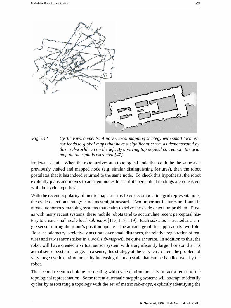
5 Mobile Robot Localization 227
irrelevant detail. When the robot arrives at a topological node that could be the same as apreviously visited and mapped node (e.g. similar distinguishing features), then the robotpostulates that it has indeed returned to the same node. To check this hypothesis, the robotexplicitly plans and moves to adjacent nodes to see if its perceptual readings are consistentwith the cycle hypothesis.
With the recent popularity of metric maps such as fixed decomposition grid representations,the cycle detection strategy is not as straightforward. Two important features are found inmost autonomous mapping systems that claim to solve the cycle detection problem. First,as with many recent systems, these mobile robots tend to accumulate recent perceptual his-tory to create small-scale local sub-maps [117, 118, 119]. Each sub-map is treated as a sin-gle sensor during the robot’s position update. The advantage of this approach is two-fold.Because odometry is relatively accurate over small distances, the relative registration of fea-tures and raw sensor strikes in a local sub-map will be quite accurate. In addition to this, therobot will have created a virtual sensor system with a significantly larger horizon than itsactual sensor system’s range. In a sense, this strategy at the very least defers the problem ofvery large cyclic environments by increasing the map scale that can be handled well by therobot.
The second recent technique for dealing with cycle environments is in fact a return to thetopological representation. Some recent automatic mapping systems will attempt to identifycycles by associating a topology with the set of metric sub-maps, explicitly identifying the
Fig 5.42 Cyclic Environments: A naive, local mapping strategy with small local er-ror leads to global maps that have a significant error, as demonstrated bythis real-world run on the left. By applying topological correction, the gridmap on the right is extracted [47].
R. Siegwart, EPFL, Illah Nourbakhsh, CMU

228 Autonomous Mobile Robots
loops first at the topological level. In the case of [118] for example, the topological levelloop is identified by a human who pushes a button at a known landmark position. In the caseof [119] the topological level loop is determined by performing correspondence tests be-tween sub-maps, postulating that two sub-maps represent the same place in the environmentwhen the correspondence is good.
One could certainly imagine other augmentations based on known topological methods. Forexample, the globally unique localization methods described in Section (5.7) could be usedto identify topological correctness. It is notable that the automatic mapping research of thepresent has, in many ways, returned to the basic topological correctness question that was atthe heart of some of the earliest automatic mapping research in mobile robotics more than adecade ago. Of course, unlike that early work, today’s automatic mapping results boast cor-rect cycle detection combined with high-fidelity geometric maps of the environment.
5.8.2.2 Dynamic environments
A second challenge extends not just to existing automonous mapping solutions but even tothe basic formulation of the stochastic map approach. All of these strategies tend to assumethat the environment is either unchanging or changes in ways that are virtually insignificant.Such assumptions are certainly valid with respect to some environments, such as for exam-ple the computer science department of a university at 3:00 past midnight. However, in agreat many cases this assumption is incorrect. In the case of wide-open spaces that are pop-ular gathering places for humans, there is rapid change in the freespace and a vast majorityof sensor strikes represent detection of the transient humans rather than fixed surfaces suchas the perimeter wall. Another class of dynamic environments are spaces such as factoryfloors and warehouses, where the objects being stored redefine the topology of the pathwayson a day-to-day basis as shipments are moved in and out.
In all such dynamic environments, an automatic mapping system should capture the salientobjects detected by its sensors and, furthermore, the robot should have the flexibility to mod-ify its map as the position of these salient objects changes. The subject of continuous map-ping, or mapping of dynamic environments is to some degree a direct outgrowth ofsuccessful strategies for automatic mapping of unfamiliar environments. For example, in
the case of stochastic mapping using the credibility factor mechanism, the credibility
equation can continue to provide feedback regarding the probability of existence of variousmapped features after the initial map creation process is ostensibly complete. Thus, a map-ping system can become a map-modifying system by simply continuing to operate. This ismost effective, of course, if the mapping system is real-time and incremental. If map con-struction requires off-line global optimization, then the desire to make small-grained, incre-mental adjustments to the map is more difficult to satisfy.
Earlier we stated that a mapping system should capture only the salient objects detected byits sensors. One common argument for handling the detection of, for instance, humans in
the environment is that mechanisms such as can take care of all features that did not de-
serve to be mapped in the first place. For example, in [117] the authors develop a systembased on a set of local occupany grids (called evidence grids) and a global occupancy grid.
ct
ct
5 Mobile Robot Localization 229
Each time the robot’s most recent local evidence grid is used to update a region of the globaloccupancy grid, extraneous occupied cells in the global occupancy grid are freed if the localoccupancy grid detected no objects (with high confidence) at those same positions.
The general solution to the problem of detecting salient features, however, begs a solutionto the perception problem in general. When a robot’s sensor system can reliably detect thedifference between a wall and a human, using for example a vision system, then the problemof mapping in dynamic environments will become significantly more straightforward.
We have discussed just two important considerations for automatic mapping. There is stilla great deal of research activity focusing on the general map building and localization prob-lem [9, 6, 47, 48, 49, 50, 75, 77]. However, there are few groups working on the generalproblem of probabilistic map building (i.e. stochastic maps) and, so far, a consistent and ab-solutely general solution has yet to be found. This field is certain to produce significant newresults in the next several years, and as the perceptual power of robots improves we expectthe payoff to be greatest here.
R. Siegwart, EPFL, Illah Nourbakhsh, CMU

230 Autonomous Mobile Robots
5 Mobile Robot Localization 159
5 Mobile Robot Localization
5.1 Introduction
Navigation is one of the most challenging competencies required of a mobile robot. Successin navigation requires success at the four building blocks of navigation (fig. 5.2): percep-tion- the robot must interpret its sensors to extract meaningful data; localization- the robotmust determine its position in the environment; cognition- the robot must decide how to actto achieve its goals; and motion control- the robot must modulate its motor outputs toachieve the desired trajectory.
Of these four components, localization has received the greatest research attention in thepast decade and, as a result, significant advances have been made on this front. In this chap-ter, we will explore the successful localization methodologies of recent years. First, Section5.2 describes how sensor and effector uncertainty is responsible for the difficulties of local-ization. Then, Section 5.3 describes two extreme approaches to dealing with the challengeof robot localization: avoiding localization altogether, and performing explicit map-basedlocalization. The remainder of the chapter discusses the question of representation, then pre-sents case studies of successful localization systems using a variety of representations andtechniques to achieve mobile robot localization competence.
Fig 5.1 Where am I?
?
R. Siegwart, EPFL, Illah Nourbakhsh, CMU
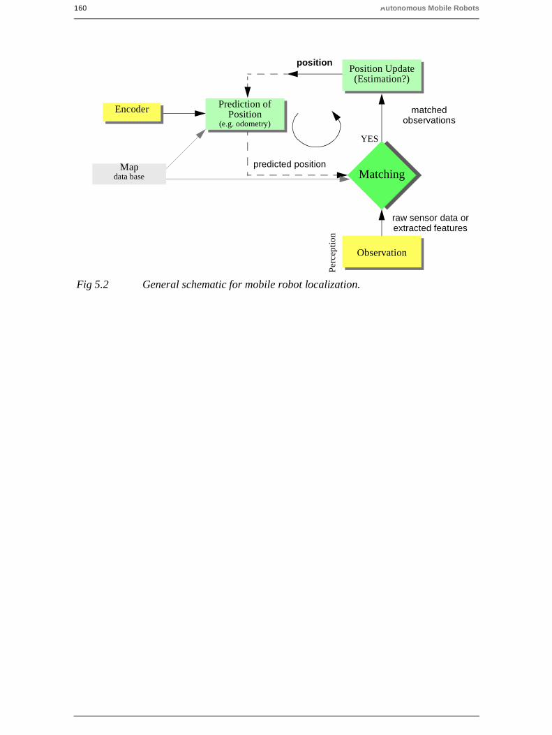
160 Autonomous Mobile Robots
Observation
Mapdata base
Prediction ofPosition
(e.g. odometry)
Fig 5.2 General schematic for mobile robot localization.
Per
cept
ion
Matching
Position Update(Estimation?)
raw sensor data orextracted features
predicted position
position
matchedobservations
YES
Encoder
5 Mobile Robot Localization 161
5.2 The Challenge of Localization: noise and aliasing
If one could attach an accurate GPS (Global Position System) sensor to a mobile robot, muchof the localization problem would be obviated. The GPS would inform the robot of its exactposition and orientation, indoors and outdoors, so that the answer to the question, "Wheream I?" would always be immediately available. Unfortunately, such a sensor is not currentlypractical. The existing GPS network provides accuracy to within several meters, which isunacceptable for localizing human-scale mobile robots as well as miniature mobile robotssuch as desk robots and the body-navigating nano-robots of the future. Furthermore, GPStechnologies cannot function indoors or in obstructed areas and are thus limited in theirworkspace.
But, looking beyond the limitations of GPS, localization implies more than knowing one’sabsolute position in the Earth’s reference frame. Consider a robot that is interacting with hu-mans. This robot may need to identify its absolute position, but its relative position with re-spect to target humans is equally important. Its localization task can include identifyinghumans using its sensor array, then computing its relative position to the humans. Further-more, during the Cognition step a robot will select a strategy for achieving its goals. If it in-tends to reach a particular location, then localization may not be enough. The robot mayneed to acquire or build an environmental model, a map, that aids it in planning a path to thegoal. Once again, localization means more than simply determining an absolute pose inspace; it means building a map, then identifying the robot’s position relative to that map.
Clearly, the robot’s sensors and effectors play an integral role in all the above forms of lo-calization. It is because of the inaccuracy and incompleteness of these sensors and effectorsthat localization poses difficult challenges. This section identifies important aspects of thissensor and effector suboptimality.
5.2.1 Sensor Noise
Sensors are the fundamental robot input for the process of perception, and therefore the de-gree to which sensors can discriminate world state is critical. Sensor noise induces a limi-tation on the consistency of sensor readings in the same environmental state and, therefore,on the number of useful bits available from each sensor reading. Often, the source of sensornoise problems is that some environmental features are not captured by the robot’s represen-tation and are thus overlooked.
For example, a vision system used for indoor navigation in an office building may use thecolor values detected by its color CCD camera. When the sun is hidden by clouds, the illu-mination of the building’s interior changes due to windows throughout the building. As aresult, hue values are not constant. The color CCD appears noisy from the robot’s perspec-tive as if subject to random error, and the hue values obtained from the CCD camera will beunusable, unless the robot is able to note the position of the Sun and clouds in its represen-tation.
Illumination dependency is only one example of the apparent noise in a vision-based sensorsystem. Picture jitter, signal gain, blooming and blurring are all additional sources of noise,potentially reducing the useful content of a color video image.
R. Siegwart, EPFL, Illah Nourbakhsh, CMU

162 Autonomous Mobile Robots
Consider the noise level (i.e. apparent random error) of ultrasonic range-measuring sensors(e.g. sonars) as we discussed in Section 4.1.2.3. When a sonar transducer emits sound to-wards a relatively smooth and angled surface, much of the signal will coherently reflectaway, failing to generate a return echo. Depending on the material characteristics, a smallamount of energy may return nonetheless. When this level is close to the gain threshold ofthe sonar sensor, then the sonar will, at times, succeed and, at other times, fail to detect theobject. From the robot’s perspective, a virtually unchanged environmental state will resultin two different possible sonar readings: one short, and one long.
The poor signal to noise ratio of a sonar sensor is further confounded by interference be-tween multiple sonar emitters. Often, research robots have between 12 to 48 sonars on a sin-gle platform. In acoustically reflective environments, multipath interference is possiblebetween the sonar emissions of one tranducer and the echo detection circuitry of anothertransducer. The result can be dramatically large errors (i.e. underestimation) in ranging val-ues due to a set of coincidental angles. Such errors occur rarely, less than 1% of the time,and are virtually random from the robot’s perspective.
In conclusion, sensor noise reduces the useful information content of sensor readings. Clear-ly, the solution is to take multiple readings into account, employing temporal fusion ormulti-sensor fusion to increase the overall information content of the robot’s inputs.
5.2.2 Sensor Aliasing
A second shortcoming of mobile robot sensors causes them to yield little information con-tent, further exacerbating the problem of perception and, thus, localization. The problem,known as sensor aliasing, is a phenomenon that humans rarely encounter. The human sen-sory system, particularly the visual system, tends to receive unique inputs in each unique lo-cal state. In other words, every different place looks different. The power of this uniquemapping is only apparent when one considers situations where this fails to hold. Considermoving through an unfamiliar building that is completely dark. When the visual system seesonly black, one’s localization system quickly degrades. Another useful example is that of ahuman-sized maze made from tall hedges. Such mazes have been created for centuries, andhumans find them extremely difficult to solve without landmarks or clues because, withoutvisual uniqueness, human localization competence degrades rapidly.
In robots, the non-uniqueness of sensors readings, or sensor aliasing, is the norm and not theexception. Consider a narrow-beam rangefinder such as ultrasonic or infrared rangefinders.This sensor provides range information in a single direction without any additional data re-garding material composition such as color, texture and hardness. Even for a robot with sev-eral such sensors in an array, there are a variety of environmental states that would triggerthe same sensor values across the array. Formally, there is a many-to-one mapping from en-vironmental states to the robot’s perceptual inputs. Thus, the robot’s percepts cannot distin-guish from among these many states. A classical problem with sonar-based robots involvesdistinguishing between humans and inanimate objects in an indoor setting. When facing anapparent obstacle in front of itself, should the robot say "Excuse me" because the obstaclemay be a moving human, or should the robot plan a path around the object because it maybe a cardboard box? With sonar alone, these states are aliased and differentiation is impos-
5 Mobile Robot Localization 163
sible.
The problem posed to navigation because of sensor aliasing is that, even with noise-free sen-sors, the amount of information is generally insufficient to identify the robot’s position froma single percept reading. Thus techniques must be employed by the robot programmer thatbase the robot’s localization on a series of readings and, thus, sufficient information to re-cover the robot’s position over time.
5.2.3 Effector Noise
The challenges of localization do not lie with sensor technologies alone. Just as robot sen-sors are noisy, limiting the information content of the signal, so robot effectors are alsonoisy. In particular, a single action taken by a mobile robot may have several different pos-sible results, even though from the robot’s point of view the initial state before the actionwas taken is well-known.
In short, mobile robot effectors introduce uncertainty about future state. Therefore the sim-ple act of moving tends to increase the uncertainty of a mobile robot. There are, of course,exceptions. Using cognition, the motion can be carefully planned so as to minimize this ef-fect, and indeed sometimes to actually result in more certainty. Furthermore, when the robotactions are taken in concert with careful interpretation of sensory feedback, it can compen-sate for the uncertainty introduced by noisy actions using the information provided by thesensors.
First, however, it is important to understand the precise nature of the effector noise that im-pacts mobile robots. It is important to note that, from the robot’s point of view, this error inmotion is viewed as error in odometry, or the robot’s inability to estimate its own positionover time using knowledge of its kinematics and dynamics. The true source of error gener-ally lies in an incomplete model of the environment. For instance, the robot does not modelthe fact that the floor may be sloped, the wheels may slip, and a human may push the robot.All of these un-modeled sources of error result in inaccuracy between the physical motionof the robot, the intended motion of the robot and the proprioceptive sensor estimates of mo-tion.
In odometry (wheel sensors only) and dead reckoning (also heading sensors) the position up-date is based on proprioceptive sensors. The movement of the robot, sensed with wheel en-coders and /or heading sensors is integrated to compute position. Because the sensormeasurement errors are integrated, the position error accumulates over time. Thus the posi-tion has to be updated from time to time by other localization mechanisms. Otherwise therobot is not able to maintain a meaningful position estimate in long run.
In the following we will concentrate on odometry based on the wheel sensor readings of adifferential drive robot only (see also [3, 40, 41]). Using additional heading sensors (e.g. gy-roscope) can help to reduce the cumulative errors, but the main problems remain the same.
There are many sources of odometric error, from environmental factors to resolution:
• Limited resolution during integration (time increments, measurement resolution,etc.)
• Misalignment of the wheels (deterministic)
R. Siegwart, EPFL, Illah Nourbakhsh, CMU
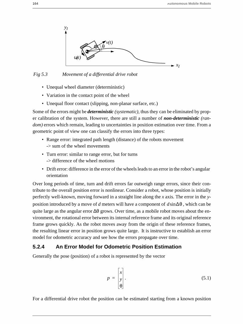
164 Autonomous Mobile Robots
• Unequal wheel diameter (deterministic)
• Variation in the contact point of the wheel
• Unequal floor contact (slipping, non-planar surface, etc.)
Some of the errors might be deterministic (systematic), thus they can be eliminated by prop-er calibration of the system. However, there are still a number of non-deterministic (ran-dom) errors which remain, leading to uncertainties in position estimation over time. From ageometric point of view one can classify the errors into three types:
• Range error: integrated path length (distance) of the robots movement-> sum of the wheel movements
• Turn error: similar to range error, but for turns-> difference of the wheel motions
• Drift error: difference in the error of the wheels leads to an error in the robot’s angularorientation
Over long periods of time, turn and drift errors far outweigh range errors, since their con-tribute to the overall position error is nonlinear. Consider a robot, whose position is initiallyperfectly well-known, moving forward in a straight line along the x axis. The error in the y-
position introduced by a move of d meters will have a component of , which can be
quite large as the angular error ∆θ grows. Over time, as a mobile robot moves about the en-vironment, the rotational error between its internal reference frame and its original referenceframe grows quickly. As the robot moves away from the origin of these reference frames,the resulting linear error in position grows quite large. It is instructive to establish an errormodel for odometric accuracy and see how the errors propagate over time.
5.2.4 An Error Model for Odometric Position Estimation
Generally the pose (position) of a robot is represented by the vector
. (5.1)
For a differential drive robot the position can be estimated starting from a known position
d ∆θsin
Fig 5.3 Movement of a differential drive robot
v(t)
ω(t)
θ
yI
xI
px
y
θ
=

5 Mobile Robot Localization 165
by integrating the movement (summing the incremental travel distances). For a discrete sys-
tem with a fixed sampling interval ∆t the incremental travel distances are:
(5.2)
(5.3)
(5.4)
(5.5)
where:
: Path traveled in the last sampling interval
: Traveled distances for right and left wheel respectively
: Distance between the two wheels of differential drive robot
Thus we get the updated position p’:
(5.6)
By using the relation for of equations (5.4) and (5.5) we further obtain the basic
equation for odometric position update (for differential drive robots):
(5.7)
As we discussed earlier, odometric position updates can give only a very rough estimate ofthe actual position. Due to integration errors of the uncertainties of p and the motion errors
during the incremental motion the position error based on odometry integration
grows with time.
In the next step we will establish an error model for the integrated position p’ to obtain the
covariance matrix of the odometric position estimate. To do so, we assume that at the
∆x ∆y ∆θ;;( )
∆x ∆s θ ∆θ 2⁄+( )cos=
∆y ∆s θ ∆θ 2⁄+( )sin=
∆θ∆sr ∆– sl
b-------------------=
∆s∆sr ∆sl+
2----------------------=
∆x ∆y ∆θ;;( )
∆sr ∆sl;
b
p'x'
y'
θ'p∆s θ ∆θ 2⁄+( )cos
∆s θ ∆θ 2⁄+( )sin
∆θ
+x
y
θ
∆s θ ∆θ 2⁄+( )cos
∆s θ ∆θ 2⁄+( )sin
∆θ
+= = =
∆s ∆θ;( )
p' f x y θ ∆sr ∆sl, , , ,( )x
y
θ
∆sr ∆sl+
2---------------------- θ
∆sr ∆– sl
2b-------------------+
cos
∆sr ∆sl+
2---------------------- θ
∆sr ∆– sl
2b-------------------+
sin
∆sr ∆– sl
b-------------------
+= =
∆sr ∆sl;( )
Σp'
R. Siegwart, EPFL, Illah Nourbakhsh, CMU

166 Autonomous Mobile Robots
starting point the initial covariance matrix is known. For the motion increment
we assume the following covariance matrix :
(5.8)
where and are the distances travelled by each wheel, and , are error constants
representing the non-deterministic parameters of the motor drive and the wheel-floor inter-action. As you can see in equation (5.8) we made the following assumption:
• The two errors of the individually driven wheels are independent1
• The errors are proportional to the absolute value of the traveled distances .
These assumptions, while not perfect, are suitable and will thus be used for the further de-velopment of the error model. The motion errors are due to unprecise movement because ofdeformation of wheel, slippage, unequal floor, errors in encoders, et cetera. The values for
the error constants and depend on the robot and the environment and should be exper-
imentally established by performing and analyzing representative movements.
If we assume that p and are uncorrelated and the derivation of f (equ. (5.7))
is reasonably approximated by the first order Taylor expansion (linearization) we conclude,using the error propagation law (see section 4.2.3):
(5.9)
The covariance matrix is, of course, always given by the of the previous step, and
can thus be calculated after specifying an initial value (e.g. 0).
Using equation (5.7) we can develop the two Jacobians and :
(5.10)
1. If there is more knowledge regarding the actual robot kinematics, the correlation terms of the covariance matrixcould also be used.
Σp
∆sr ∆sl;( ) Σ∆
Σ∆ covar ∆sr ∆sl,( )kr ∆sr 0
0 kl ∆sl
= =
∆sr ∆sl kr kl
∆sr ∆sl;( )
kr kl
∆rl ∆sr ∆sl;( )=
Σp' ∇ pf Σp ∇⋅pfT⋅ ∇ ∆rl
f Σ∆ ∇ ∆rlf⋅ T⋅+=
Σp Σp'
Fp ∇ pf= F∆rl∇ ∆rl
f=
Fp ∇ pf ∇ p fT( ) f∂
x∂----- f∂
y∂----- f∂θ∂
------1 0 ∆s θ ∆θ 2⁄+( )sin–
0 1 ∆s θ ∆θ 2⁄+( )cos
0 0 1
= = = =

5 Mobile Robot Localization 167
(5.11)
The details for arriving at equation (5.11) are:
(5.12)
(5.13)
and with
; (5.14)
; ; ; (5.15)
we obtain equation (5.11).
Figures 5.4 and 5.5 show typical examples of how the position errors grow with time. Theresults have been computed using the error model presented above.
Once the error model has been established, the error parameters must be specified. One cancompensate for deterministic errors properly calibrating the robot. However the error pa-rameters specifying the non-deterministic errors can only be quantified by statistical (repet-itive) measurements. A detailed discussion of odometric errors and a method for calibrationand quantification of deterministic and non-deterministic errors can be found in [4].
F∆rl
12--- θ ∆θ 2⁄+( ) ∆s
2b------ θ ∆θ 2⁄+( )sin–cos
12--- θ ∆θ 2⁄+( ) ∆s
2b------ θ ∆θ 2⁄+( )sin+cos
12--- θ ∆θ 2⁄+( ) ∆s
2b------ θ ∆θ 2⁄+( )cos+sin
12--- θ ∆θ 2⁄+( ) ∆s
2b------– θ ∆θ 2⁄+( )cossin
1b--- 1
b---–
=
F∆rl∇ ∆rl
f f∂∆sr∂
----------- f∂∆sl∂
---------- …= = =
…
∆s∂∆sr∂
------------ θ ∆θ 2⁄+( ) θ ∆θ 2⁄+( )sin–( ) ∆θ∂∆sr∂------------+cos
∆s∂∆sl∂
------------ θ ∆θ 2⁄+( ) θ ∆θ 2⁄+( )sin–( ) ∆θ∂∆sl∂------------+cos
∆s∂∆sr∂
------------ θ ∆θ 2⁄+( ) θ ∆θ 2⁄+( )cos( ) ∆θ∂∆sr∂------------+sin
∆s∂∆sl∂
------------ θ ∆θ 2⁄+( ) θ ∆θ 2⁄+( )cos( ) ∆θ∂∆sl∂------------+sin
∆θ∂∆sr∂
------------ ∆θ∂∆sl∂
------------
=
∆s∆sr ∆sl+
2----------------------= ∆θ
∆sr ∆– sl
b-------------------=
∆s∂∆sr∂
----------- 12---=
∆s∂∆sl∂
---------- 12---=
∆θ∂∆sr∂
----------- 1b---=
∆θ∂∆sl∂
---------- 1b---–=
R. Siegwart, EPFL, Illah Nourbakhsh, CMU
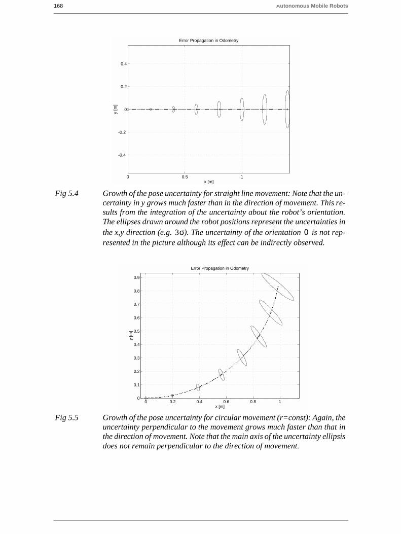
168 Autonomous Mobile Robots
Fig 5.4 Growth of the pose uncertainty for straight line movement: Note that the un-certainty in y grows much faster than in the direction of movement. This re-sults from the integration of the uncertainty about the robot’s orientation.The ellipses drawn around the robot positions represent the uncertainties inthe x,y direction (e.g. ). The uncertainty of the orientation is not rep-resented in the picture although its effect can be indirectly observed.
3σ θ
0 0.5 1
-0.4
-0.2
0
0.2
0.4
Error Propagation in Odometry
x [m]
y [m
]
Fig 5.5 Growth of the pose uncertainty for circular movement (r=const): Again, theuncertainty perpendicular to the movement grows much faster than that inthe direction of movement. Note that the main axis of the uncertainty ellipsisdoes not remain perpendicular to the direction of movement.
0 0.2 0.4 0.6 0.8 10
0.1
0.2
0.3
0.4
0.5
0.6
0.7
0.8
0.9
Error Propagation in Odometry
x [m]
y [m
]
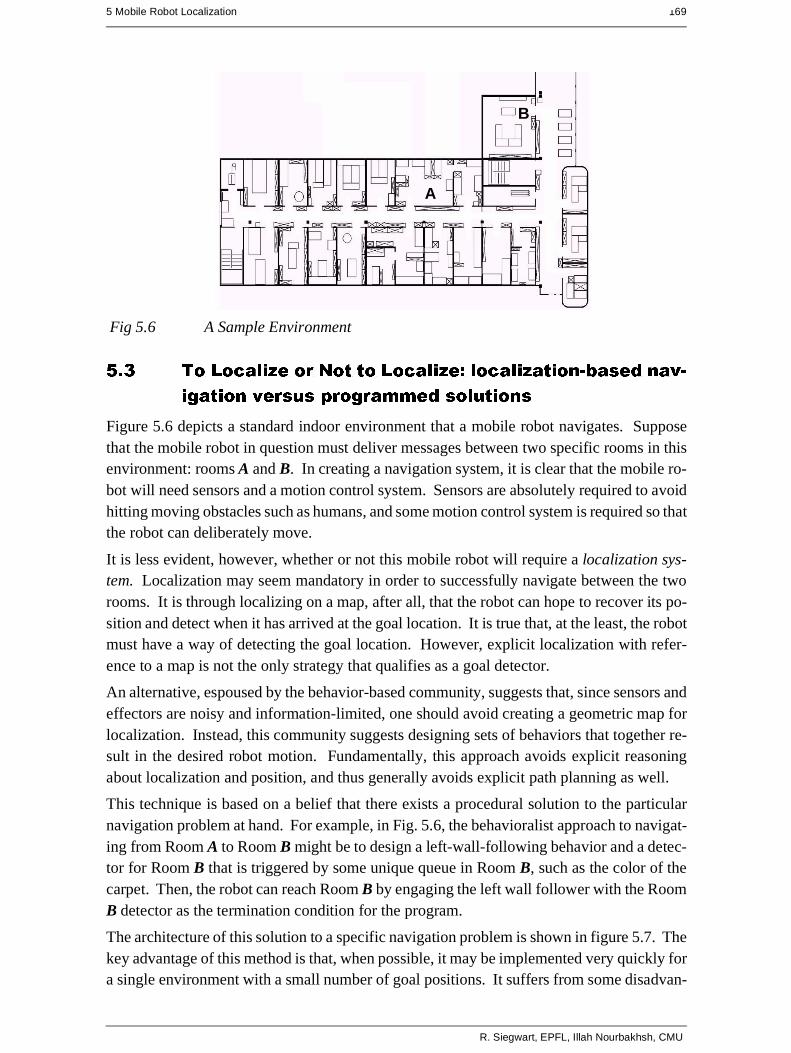
5 Mobile Robot Localization 169
5.3 To Localize or Not to Localize: localization-based nav-
igation versus programmed solutions
Figure 5.6 depicts a standard indoor environment that a mobile robot navigates. Supposethat the mobile robot in question must deliver messages between two specific rooms in thisenvironment: rooms A and B. In creating a navigation system, it is clear that the mobile ro-bot will need sensors and a motion control system. Sensors are absolutely required to avoidhitting moving obstacles such as humans, and some motion control system is required so thatthe robot can deliberately move.
It is less evident, however, whether or not this mobile robot will require a localization sys-tem. Localization may seem mandatory in order to successfully navigate between the tworooms. It is through localizing on a map, after all, that the robot can hope to recover its po-sition and detect when it has arrived at the goal location. It is true that, at the least, the robotmust have a way of detecting the goal location. However, explicit localization with refer-ence to a map is not the only strategy that qualifies as a goal detector.
An alternative, espoused by the behavior-based community, suggests that, since sensors andeffectors are noisy and information-limited, one should avoid creating a geometric map forlocalization. Instead, this community suggests designing sets of behaviors that together re-sult in the desired robot motion. Fundamentally, this approach avoids explicit reasoningabout localization and position, and thus generally avoids explicit path planning as well.
This technique is based on a belief that there exists a procedural solution to the particularnavigation problem at hand. For example, in Fig. 5.6, the behavioralist approach to navigat-ing from Room A to Room B might be to design a left-wall-following behavior and a detec-tor for Room B that is triggered by some unique queue in Room B, such as the color of thecarpet. Then, the robot can reach Room B by engaging the left wall follower with the RoomB detector as the termination condition for the program.
The architecture of this solution to a specific navigation problem is shown in figure 5.7. Thekey advantage of this method is that, when possible, it may be implemented very quickly fora single environment with a small number of goal positions. It suffers from some disadvan-
Fig 5.6 A Sample Environment
A
B
R. Siegwart, EPFL, Illah Nourbakhsh, CMU

170 Autonomous Mobile Robots
tages, however. First, the method does not directly scale to other environments or to largerenvironments. Often, the navigation code is location-specific, and the same degree of cod-ing and debugging is required to move the robot to a new environment.
Second, the underlying procedures, such as left-wall-follow, must be carefully designed toproduce the desired behavior. This task may be time-consuming and is heavily dependenton the specific robot hardware and environmental characteristics.
Third, a behavior-based system may have multiple active behaviors at any one time. Evenwhen individual behaviors are tuned to optimize performance, this fusion and rapid switch-ing between multiple behaviors can negate that fine-tuning. Often, the addition of each newincremental behavior forces the robot designer to re-tune all of the existing behaviors againto ensure that the new interactions with the freshly introduced behavior are all stable.
In contrast to the behavior-based approach, the map-based approach includes both localiza-tion and cognition modules (see Fig. 5.8). In map-based navigation, the robot explicitly at-tempts to localize by collecting sensor data, then updating some belief about its position withrespect to a map of the environment. The key advantages of the map-based approach fornavigation are as follows:
• The explicit, map-based concept of position makes the system’s belief about positiontransparently available to the human operators.
• The existence of the map itself represents a medium for communication between hu-man and robot: the human can simply give the robot a new map if the robot goes to
Fig 5.7 An Architecture for Behavior-based Navigation
sensors detect goal position
discover new area
avoid obstacles
follow right / left wall
communicate data
actuators
coordination / fusione.g. fusion via vector summation
Σ
Fig 5.8 An Architecture for Map-based (or model-based) Navigation
sensors
cognition / planning
localization / map-building
motion control
perception
actuators

5 Mobile Robot Localization 171
a new environment.
• The map, if created by the robot, can be used by humans as well, achieving two uses.
The map-based approach will require more up-front development effort to create a navigat-ing mobile robot. The hope is that the development effort results in an architecture that cansuccessfully map and navigate a variety of environments, thereby amortizing the up-frontdesign cost over time.
Of course the key risk of the map-based approach is that an internal representation, ratherthan the real world itself, is being constructed and trusted by the robot. If that model diverg-es from reality (i.e. if the map is wrong), then the robot’s behavior may be undesirable, evenif the raw sensor values of the robot are only transiently incorrect.
In the remainder of this chapter, we focus on a discussion of map-based approaches and, spe-cifically, the localization component of these techniques. These approaches are particularlyappropriate for study given their significant recent successes in enabling mobile robots tonavigate a variety of environments, from academic research buildings to factory floors andmuseums around the world.
R. Siegwart, EPFL, Illah Nourbakhsh, CMU

172 Autonomous Mobile Robots
5.4 Belief Representation
The fundamental issue that differentiates various map-based localization systems is the issueof representation. There are two specific concepts that the robot must represent, and eachhas its own unique possible solutions. The robot must have a representation (a model) ofthe environment, or a map. What aspects of the environment are contained in this map? Atwhat level of fidelity does the map represent the environment? These are the design ques-tions for map representation.
The robot must also have a representation of its belief regarding its position on the map.Does the robot identify a single unique position as its current position, or does it describe itsposition in terms of a set of possible positions? If multiple possible positions are expressedin a single belief, how are those multiple positions ranked, if at all? These are the designquestions for belief representation.
Decisions along these two design axes can result in varying levels of architectural complex-ity, computational complexity and overall localization accuracy. We begin by discussingbelief representation. The first major branch in a taxonomy of belief representation systemsdifferentiates between single hypothesis and multiple hypothesis belief systems. The formercovers solutions in which the robot postulates its unique position, whereas the latter enablesa mobile robot to describe the degree to which it is uncertain about its position. A samplingof different belief and map representations is shown in figure 5.9.
5.4.1 Single Hypothesis Belief
The single hypothesis belief representation is the most direct possible postulation of mobilerobot position. Given some environmental map, the robot’s belief about position is ex-pressed as a single unique point on the map. In Fig. 5.10, three examples of a single hypoth-esis belief are shown using three different map representations of the same actualenvironment (fig. 5.10a). In 5.10b, a single point is geometrically annotated as the robot’sposition in a continuous two-dimensional geometric map. In 5.10c, the map is a discrete,tessellated map, and the position is noted at the same level of fidelity as the map cell size.In 5.10d, the map is not geometrical at all but abstract and topological. In this case, the sin-gle hypothesis of position involves identifying a single node i in the topological graph as therobot’s position.
The principal advantage of the single hypothesis representation of position stems from thefact that, given a unique belief, there is no position ambiguity. The unambiguous nature ofthis representation facilitates decision-making at the robot’s cognitive level (e.g. path plan-ning). The robot can simply assume that its belief is correct, and can then select its futureactions based on its unique position.
Just as decision-making is facilitated by a single-position hypothesis, so updating the robot’sbelief regarding position is also facilitated, since the single position must be updated by def-inition to a new, single position. The challenge with this position update approach, whichultimately is the principal disadvantage of single-hypothesis representation, is that robotmotion often induces uncertainty due to effectory and sensory noise. Therefore, forcing theposition update process to always generate a single hypothesis of position is challenging

5 Mobile Robot Localization 173
and, often, impossible.
5.4.2 Multiple Hypothesis Belief
In the case of multiple hypothesis beliefs regarding position, the robot tracks not just a singlepossible position but a possibly infinite set of positions.
In one simple example originating in the work of Jean-Claude Latombe [5, 89], the robot’sposition is described in terms of a convex polygon positioned in a two-dimensional map ofthe environment. This multiple hypothesis representation communicates the set of possiblerobot positions geometrically, with no preference ordering over the positions. Each point in
Fig 5.9 Belief representation regarding the robot position (1 dimensional) in con-tinuous and discretized (tessellated) maps.a)Continuous map with multiple hypothesis belief, e.g. single Gaussian cen-tered at a single continuous valueb)Continuous map with multiple hypothesis belief, e.g. multiple Gaussianscentered at multiple continuous valuesc)Discretized (decomposed) grid map with probability values for all possi-ble robot position, e.g. Markov approachd)Discretized topological map with probability value for all possible nodes(topological robot positions), e.g. Markov approach
position x
prob
abili
tyP
position x
prob
abili
tyP
position x
prob
abili
tyP
a
b
c
node
prob
abili
tyP
d
A B C D E F G
of topological map
R. Siegwart, EPFL, Illah Nourbakhsh, CMU

174 Autonomous Mobile Robots
the map is simply either contained by the polygon and, therefore, in the robot’s belief set, oroutside the polygon and thereby excluded. Mathematically, the position polygon serves topartition the space of possible robot positions. Such a polygonal representation of the mul-tiple hypothesis belief can apply to a continuous, geometric map of the environment or, al-ternatively, to a tessellated, discrete approximation to the continuous environment.
It may be useful, however, to incorporate some ordering on the possible robot positions, cap-turing the fact that some robot positions are likelier than others. A strategy for representinga continuous multiple hypothesis belief state along with a preference ordering over possiblepositions is to model the belief as a mathematical distribution. For example, [42,47] notatethe robot’s position belief using an {X,Y} point in the two-dimensional environment as the
mean plus a standard deviation parameter , thereby defining a Gaussian distribution.
The intended interpretation is that the distribution at each position represents the probability
Fig 5.10 Three examples of single hypotheses of position using different map repre-sentation.a) real map with walls, doors and furnitureb) line-based map
-> around 100 lines with two parametersc) occupancy grid based map
-> around 3000 gird cells sizing 50x50 cmd) topological map using line features (Z/S-lines) and doors
-> around 50 features and 18 nodes
node
i
a)
c)
b)
d)
(x,y,θ)robot position
µ σ
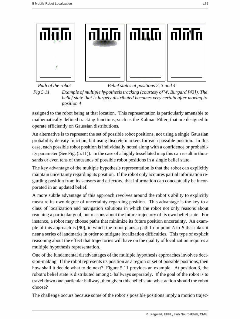
5 Mobile Robot Localization 175
assigned to the robot being at that location. This representation is particularly amenable tomathematically defined tracking functions, such as the Kalman Filter, that are designed tooperate efficiently on Gaussian distributions.
An alternative is to represent the set of possible robot positions, not using a single Gaussianprobability density function, but using discrete markers for each possible position. In thiscase, each possible robot position is individually noted along with a confidence or probabil-ity parameter (See Fig. (5.11)). In the case of a highly tessellated map this can result in thou-sands or even tens of thousands of possible robot positions in a single belief state.
The key advantage of the multiple hypothesis representation is that the robot can explicitlymaintain uncertainty regarding its position. If the robot only acquires partial information re-garding position from its sensors and effectors, that information can conceptually be incor-porated in an updated belief.
A more subtle advantage of this approach revolves around the robot’s ability to explicitlymeasure its own degree of uncertainty regarding position. This advantage is the key to aclass of localization and navigation solutions in which the robot not only reasons aboutreaching a particular goal, but reasons about the future trajectory of its own belief state. Forinstance, a robot may choose paths that minimize its future position uncertainty. An exam-ple of this approach is [90], in which the robot plans a path from point A to B that takes itnear a series of landmarks in order to mitigate localization difficulties. This type of explicitreasoning about the effect that trajectories will have on the quality of localization requires amultiple hypothesis representation.
One of the fundamental disadvantages of the multiple hypothesis approaches involves deci-sion-making. If the robot represents its position as a region or set of possible positions, thenhow shall it decide what to do next? Figure 5.11 provides an example. At position 3, therobot’s belief state is distributed among 5 hallways separately. If the goal of the robot is totravel down one particular hallway, then given this belief state what action should the robotchoose?
The challenge occurs because some of the robot’s possible positions imply a motion trajec-
Fig 5.11 Example of multiple hypothesis tracking (courtesy of W. Burgard [43]). Thebelief state that is largely distributed becomes very certain after moving toposition 4
Belief states at positions 2, 3 and 4Path of the robot
R. Siegwart, EPFL, Illah Nourbakhsh, CMU
176 Autonomous Mobile Robots
tory that is inconsistent with some of its other possible positions. One approach that we willsee in the case studies below is to assume, for decision-making purposes, that the robot isphysically at the most probable location in its belief state, then to choose a path based onthat current position. But this approach demands that each possible position have an asso-ciated probability.
In general, the right approach to such a decision-making problems would be to decide ontrajectories that eliminate the ambiguity explicitly. But this leads us to the second major dis-advantage of the multiple hypothesis approaches. In the most general case, they can be com-putationally very expensive. When one reasons in a three dimensional space of discretepossible positions, the number of possible belief states in the single hypothesis case is lim-ited to the number of possible positions in the 3D world. Consider this number to be N.When one moves to an arbitrary multiple hypothesis representation, then the number of pos-
sible belief states is the power set of N, which is far larger: . Thus explicit reasoning
about the possible trajectory of the belief state over time quickly becomes computationallyuntenable as the size of the environment grows.
There are, however, specific forms of multiple hypothesis representations that are somewhatmore constrained, thereby avoiding the computational explosion while allowing a limitedtype of multiple hypothesis belief. For example, if one assumes a Gaussian distribution ofprobability centered at a single position, then the problem of representation and tracking ofbelief becomes equivalent to Kalman Filtering, a straightforward mathematical process de-scribed below. Alternatively, a highly tessellated map representation combined with a limitof 10 possible positions in the belief state, results in a discrete update cycle that is, at worst,only 10x more computationally expensive than single hypothesis belief update.
In conclusion, the most critical benefit of the multiple hypothesis belief state is the ability tomaintain a sense of position while explicitly annotating the robot’s uncertainty about its ownposition. This powerful representation has enabled robots with limited sensory informationto navigate robustly in an array of environments, as we shall see in the case studies below.
2N

5 Mobile Robot Localization 177
5.5 Map Representation
The problem of representing the environment in which the robot moves is a dual of the prob-lem of representing the robot’s possible position or positions. Decisions made regarding theenvironmental representation can have impact on the choices available for robot positionrepresentation. Often the fidelity of the position representation is bounded by the fidelity ofthe map.
Three fundamental relationships must be understood when choosing a particular map repre-sentation:
• The precision of the map must appropriately match the precision with which the ro-bot needs to achieve its goals.
• The precision of the map and the type of features represented must match the preci-sion and data types returned by the robot’s sensors.
• The complexity of the map representation has direct impact on the computationalcomplexity of reasoning about mapping, localization and navigation.
In the following sections, we identify and discuss critical design choices in creating a maprepresentation. Each such choice has great impact on the relationships listed above and onthe resulting robot localization architecture. As we will see, the choice of possible map rep-resentations is broad. Selecting an appropriate representation requires understanding all ofthe trade-offs inherent in that choice as well as understanding the specific context in whicha particular mobile robot implementation must perform localization. In general, the environ-ment representation and model can be roughly classified as presented in chapter 4.3.
5.5.1 Continuous Representations
A continuous-valued map is one method for exact decomposition of the environment. Theposition of environmental features can be annoted precisely in continuous space. Mobile ro-bot implementations to date use continuous maps only in two dimensional representations,as further dimensionality can result in computational explosion.
A common approach is to combine the exactness of a continuous representation with thecompactness of the closed world assumption. This means that one assumes that the repre-sentation will specify all environmental objects in the map, and that any area in the map thatis devoid of objects has no objects in the corresponding portion of the environment. Thus,the total storage needed in the map is proportional to the density of objects in the environ-ment, and a sparse environment can be represented by a low-memory map.
One example of such a representation, shown in Figure 5.12, is a 2D representation in whichpolygons represent all obstacles in a continuos-valued coordinate space. This is similar tothe method used by Latombe [5, 113] and others to represent environments for mobile robotpath planning techniques.
In the case of [5, 113], most of the experiments are in fact simulations run exclusively withinthe computer’s memory. Therefore, no real effort would have been expended to attempt touse sets of polygons to describe a real-world environment, such as a park or office building.
R. Siegwart, EPFL, Illah Nourbakhsh, CMU
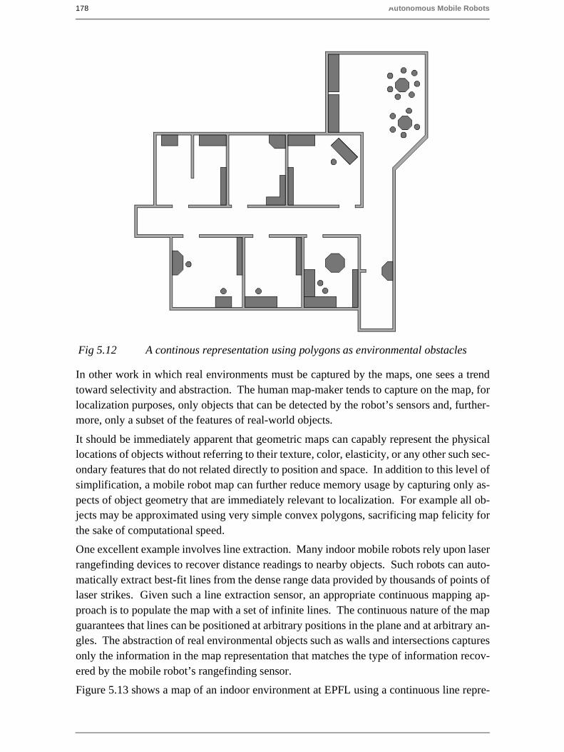
178 Autonomous Mobile Robots
In other work in which real environments must be captured by the maps, one sees a trendtoward selectivity and abstraction. The human map-maker tends to capture on the map, forlocalization purposes, only objects that can be detected by the robot’s sensors and, further-more, only a subset of the features of real-world objects.
It should be immediately apparent that geometric maps can capably represent the physicallocations of objects without referring to their texture, color, elasticity, or any other such sec-ondary features that do not related directly to position and space. In addition to this level ofsimplification, a mobile robot map can further reduce memory usage by capturing only as-pects of object geometry that are immediately relevant to localization. For example all ob-jects may be approximated using very simple convex polygons, sacrificing map felicity forthe sake of computational speed.
One excellent example involves line extraction. Many indoor mobile robots rely upon laserrangefinding devices to recover distance readings to nearby objects. Such robots can auto-matically extract best-fit lines from the dense range data provided by thousands of points oflaser strikes. Given such a line extraction sensor, an appropriate continuous mapping ap-proach is to populate the map with a set of infinite lines. The continuous nature of the mapguarantees that lines can be positioned at arbitrary positions in the plane and at arbitrary an-gles. The abstraction of real environmental objects such as walls and intersections capturesonly the information in the map representation that matches the type of information recov-ered by the mobile robot’s rangefinding sensor.
Figure 5.13 shows a map of an indoor environment at EPFL using a continuous line repre-
Fig 5.12 A continous representation using polygons as environmental obstacles
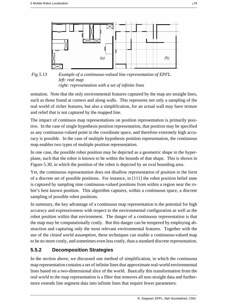
5 Mobile Robot Localization 179
sentation. Note that the only environmental features captured by the map are straight lines,such as those found at corners and along walls. This represents not only a sampling of thereal world of richer features, but also a simplification, for an actual wall may have textureand relief that is not captured by the mapped line.
The impact of continuos map representations on position representation is primarily posi-tive. In the case of single hypothesis position representation, that position may be specifiedas any continuous-valued point in the coordinate space, and therefore extremely high accu-racy is possible. In the case of multiple hypothesis position representation, the continuousmap enables two types of multiple position representation.
In one case, the possible robot position may be depicted as a geometric shape in the hyper-plane, such that the robot is known to be within the bounds of that shape. This is shown inFigure 5.30, in which the position of the robot is depicted by an oval bounding area.
Yet, the continuous representation does not disallow representation of position in the formof a discrete set of possible positions. For instance, in [111] the robot position belief stateis captured by sampling nine continuous-valued positions from within a region near the ro-bot’s best known position. This algorithm captures, within a continuous space, a discretesampling of possible robot positions.
In summary, the key advantage of a continuous map representation is the potential for highaccuracy and expressiveness with respect to the environmental configuration as well as therobot position within that environment. The danger of a continuous representation is thatthe map may be computationally costly. But this danger can be tempered by employing ab-straction and capturing only the most relevant environmental features. Together with theuse of the closed world assumption, these techniques can enable a continuous-valued mapto be no more costly, and sometimes even less costly, than a standard discrete representation.
5.5.2 Decomposition Strategies
In the section above, we discussed one method of simplification, in which the continuousmap representation contains a set of infinite lines that approximate real-world environmentallines based on a two-dimensional slice of the world. Basically this transformation from thereal world to the map representation is a filter that removes all non-straight data and further-more extends line segment data into infinite lines that require fewer parameters.
Fig 5.13 Example of a continuous-valued line representation of EPFL.left: real mapright: representation with a set of infinite lines
R. Siegwart, EPFL, Illah Nourbakhsh, CMU

180 Autonomous Mobile Robots
A more dramatic form of simplification is abstraction: a general decomposition and selec-tion of environmental features. In this section, we explore decomposition as applied in itsmore extreme forms to the question of map representation.
Why would one radically decompose the real environment during the design of a map rep-resentation? The immediate disadvantage of decomposition and abstraction is the loss offidelity between the map and the real world. Both qualitatively, in terms of overall structure,and quantitatively, in terms of geometric precision, a highly abstract map does not comparefavorably to a high-fidelity map.
Despite this disadvantage, decomposition and abstraction may be useful if the abstractioncan be planned carefully so as to capture the relevant, useful features of the world while dis-carding all other features. The advantage of this approach is that the map representation canpotentially be minimized. Furthermore, if the decomposition is hierarchical, such as in apyramid of recursive abstraction, then reasoning and planning with respect to the map rep-resentation may be computationally far superior to planning in a fully detailed world model.
A standard, lossless form of opportunistic decomposition is termed exact cell decomposi-tion. This method, introduced by [5], achieves decomposition by selecting boundaries be-tween discrete cells based on geometric criticality.
Figure 5.14 depicts an exact decomposition of a planar workspace populated by polygonalobstacles. The map representation tessellates the space into areas of free space. The repre-sentation can be extremely compact because each such area is actually stored as a singlenode, shown in the graph at the bottom of Figure 5.14.
The underlying assumption behind this decomposition is that the particular position of a ro-
Fig 5.14 Example of exact celldecomposition.

5 Mobile Robot Localization 181
bot within each area of free space does not matter. What matters is the robot’s ability totraverse from each area of free space to the adjacent areas. Therefore, as with other repre-sentations we will see, the resulting graph captures the adjacency of map locales. If indeedthe assumptions are valid and the robot does not care about its precise position within a sin-gle area, then this can be an effective representation that nonetheless captures the connec-tivity of the environment.
Such an exact decomposition is not always appropriate. Exact decomposition is a functionof the particular environment obstacles and free space. If this information is expensive tocollect or even unknown, then such an approach is not feasible.
An alternative is fixed decomposition, in which the world is tessellated, transforming thecontinuos real environment into a discrete approximation for the map. Such a transforma-tion is demonstrated in Figure 5.15, which depicts what happens to obstacle-filled and freeareas during this transformation. The key disadvantage of this approach stems from its in-exact nature. It is possible for narrow passageways to be lost during such a transformation,as shown in Figure 5.15. Formally this means that fixed decomposition is sound but notcomplete. Yet another approach is adaptive cell decomposition as presented in Figure 5.16.
The concept of fixed decomposition is extremely popular in mobile robotics; it is perhapsthe single most common map representation technique currently utilized. One very popular
Fig 5.15 Fixed decomposition of the same space. (narrow passage disappears)
R. Siegwart, EPFL, Illah Nourbakhsh, CMU
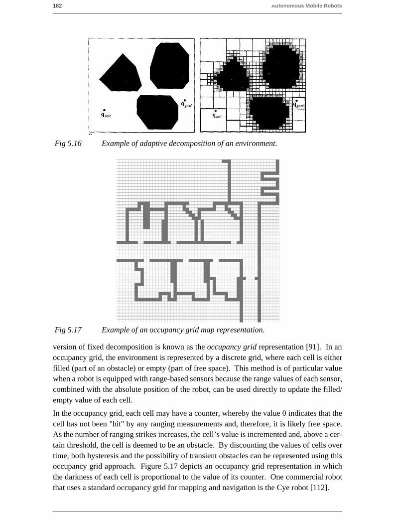
182 Autonomous Mobile Robots
version of fixed decomposition is known as the occupancy grid representation [91]. In anoccupancy grid, the environment is represented by a discrete grid, where each cell is eitherfilled (part of an obstacle) or empty (part of free space). This method is of particular valuewhen a robot is equipped with range-based sensors because the range values of each sensor,combined with the absolute position of the robot, can be used directly to update the filled/empty value of each cell.
In the occupancy grid, each cell may have a counter, whereby the value 0 indicates that thecell has not been "hit" by any ranging measurements and, therefore, it is likely free space.As the number of ranging strikes increases, the cell’s value is incremented and, above a cer-tain threshold, the cell is deemed to be an obstacle. By discounting the values of cells overtime, both hysteresis and the possibility of transient obstacles can be represented using thisoccupancy grid approach. Figure 5.17 depicts an occupancy grid representation in whichthe darkness of each cell is proportional to the value of its counter. One commercial robotthat uses a standard occupancy grid for mapping and navigation is the Cye robot [112].
Fig 5.16 Example of adaptive decomposition of an environment.
Fig 5.17 Example of an occupancy grid map representation.
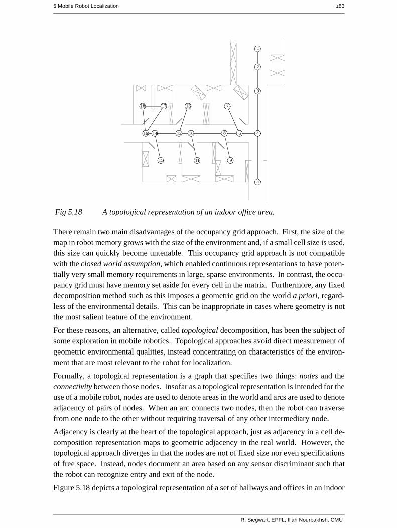
5 Mobile Robot Localization 183
There remain two main disadvantages of the occupancy grid approach. First, the size of themap in robot memory grows with the size of the environment and, if a small cell size is used,this size can quickly become untenable. This occupancy grid approach is not compatiblewith the closed world assumption, which enabled continuous representations to have poten-tially very small memory requirements in large, sparse environments. In contrast, the occu-pancy grid must have memory set aside for every cell in the matrix. Furthermore, any fixeddecomposition method such as this imposes a geometric grid on the world a priori, regard-less of the environmental details. This can be inappropriate in cases where geometry is notthe most salient feature of the environment.
For these reasons, an alternative, called topological decomposition, has been the subject ofsome exploration in mobile robotics. Topological approaches avoid direct measurement ofgeometric environmental qualities, instead concentrating on characteristics of the environ-ment that are most relevant to the robot for localization.
Formally, a topological representation is a graph that specifies two things: nodes and theconnectivity between those nodes. Insofar as a topological representation is intended for theuse of a mobile robot, nodes are used to denote areas in the world and arcs are used to denoteadjacency of pairs of nodes. When an arc connects two nodes, then the robot can traversefrom one node to the other without requiring traversal of any other intermediary node.
Adjacency is clearly at the heart of the topological approach, just as adjacency in a cell de-composition representation maps to geometric adjacency in the real world. However, thetopological approach diverges in that the nodes are not of fixed size nor even specificationsof free space. Instead, nodes document an area based on any sensor discriminant such thatthe robot can recognize entry and exit of the node.
Figure 5.18 depicts a topological representation of a set of hallways and offices in an indoor
Fig 5.18 A topological representation of an indoor office area.
1
2
3
4
5
6
7
8
9
10
11
12
13
14
15
16
18 17
R. Siegwart, EPFL, Illah Nourbakhsh, CMU

184 Autonomous Mobile Robots
environment. In this case, the robot is assumed to have an intersection detector, perhaps us-ing sonar and vision to find intersections between halls and between halls and rooms. Notethat nodes capture geometric space and arcs in this representation simply represent connec-tivity.
Another example of topological representation is the work of Dudek [49], in which the goalis to create a mobile robot that can capture the most interesting aspects of an area for humanconsumption. The nodes in Dudek’s representation are visually striking locales rather thanroute intersections.
In order to navigate using a topological map robustly, a robot must satisfy two constraints.First, it must have a means for detecting its current position in terms of the nodes of the to-pological graph. Second, it must have a means for traveling between nodes using robot mo-tion. The node sizes and particular dimensions must be optimized to match the sensorydiscrimination of the mobile robot hardware. This ability to "tune" the representation to therobot’s particular sensors can be an important advantage of the topological approach. How-ever, as the map representation drifts further away from true geometry, the expressivenessof the representation for accurately and precisely describing a robot position is lost. Thereinlies the compromise between the discrete cell-based map representations and the topologicalrepresentations. Interestingly, the continuous map representation has the potential to beboth compact like a topological representation and precise as with all direct geometric rep-resentations.
Yet, a chief motivation of the topological approach is that the environment may contain im-portant non-geometric features - features that have no ranging relevance but are useful forlocalization. In Chapter 4 we described such whole-image vision-based features.
In contrast to these whole-image feature extractors, often spatially localized landmarks areartificially placed in an environment to impose a particular visual-topological connectivityupon the environment. In effect, the artificial landmark can impose artificial structure. Ex-amples of working systems operating with this landmark-based strategy have also demon-strated success. Latombe’s landmark-based navigation research [89] has been implementedon real-world indoor mobile robots that employ paper landmarks attached to the ceiling asthe locally observable features. Chips the museum robot is another robot that uses man-made landmarks to obviate the localization problem. In this case, a bright pink square servesas a landmark with dimensions and color signature that would be hard to accidentally repro-duce in a museum environment [88]. One such museum landmark is shown in Figure (5.19).
In summary, range is clearly not the only measurable and useful environmental value for amobile robot. This is particularly true due to the advent of color vision as well as laserrangefinding, which provides reflectance information in addition to range information.Choosing a map representation for a particular mobile robot requires first understanding thesensors available on the mobile robot and second understanding the mobile robot’s function-al requirements (e.g. required goal precision and accuracy).
5.5.3 State of the Art: Current Challenges in Map Representation
The sections above describe major design decisions in regards to map representation choic-

5 Mobile Robot Localization 185
es. There are, however, fundamental real-world features that mobile robot map representa-tions do not yet represent well. These continue to be the subject of open research, andseveral such challenges are described below.
The real world is dynamic. As mobile robots come to inhabit the same spaces as humans,they will encounter moving people, cars, strollers and the transient obstacles placed andmoved by humans as they go about their activities. This is particularly true when one con-siders the home environment with which domestic robots will someday need to contend.
The map representations described above do not, in general, have explicit facilities for iden-tifying and distinguishing between permanent obstacles (e.g. walls, doorways, etc.) andtransient obstacles (e.g. humans, shipping packages, etc.). The current state of the art interms of mobile robot sensors is partly to blame for this shortcoming. Although vision re-search is rapidly advancing, robust sensors that discriminate between moving animals andstatic structures from a moving reference frame are not yet available. Furthermore, estimat-ing the motion vector of transient objects remains a research problem.
Usually, the assumption behind the above map representations is that all objects on the mapare effectively static. Partial success can be achieved by discounting mapped objects overtime. For example, occupancy grid techniques can be more robust to dynamic settings byintroducing temporal discounting, effectively treating transient obstacles as noise. The morechallenging process of map creation is particularly fragile to environment dynamics; mostmapping techniques generally require that the environment be free of moving objects duringthe mapping process. One exception to this limitation involves topological representations.Because precise geometry is not important, transient objects have little effect on the map-ping or localization process, subject to the critical constraint that the transient objects mustnot change the topological connectivity of the environment. Still, neither the occupancy gridrepresentation nor a topological approach is actively recognizing and representing transient
Fig 5.19 An artificial landmark used by Chips during autonomous docking.
R. Siegwart, EPFL, Illah Nourbakhsh, CMU

186 Autonomous Mobile Robots
objects as distinct from both sensor error and permanent map features.
As vision sensing provides more robust and more informative content regarding the tran-sience and motion details of objects in the world, mobile roboticists will in time propose rep-resentations that make use of that information. A classic example involves occlusion byhuman crowds. Museum tour guide robots generally suffer from an extreme amount of oc-clusion. If the robot’s sensing suite is located along the robot’s body, then the robot is ef-fectively blind when a group of human visitors completely surrounds the robot. This isbecause its map contains only environment features that are, at that point, fully hidden fromthe robot’s sensors by the wall of people. In the best case, the robot should recognize itsocclusion and make no effort to localize using these invalid sensor readings. In the worstcase, the robot will localize with the fully occluded data, and will update its location incor-rectly. A vision sensor that can discriminate the local conditions of the robot (e.g. we aresurrounded by people) can help eliminate this error mode.
A second open challenge in mobile robot localization involves the traversal of open spaces.Existing localization techniques generally depend on local measures such as range, therebydemanding environments that are somewhat densely filled with objects that the sensors candetect and measure. Wide open spaces such as parking lots, fields of grass and indoor atri-ums such as those found in convention centers pose a difficulty for such systems due to theirrelative sparseness. Indeed, when populated with humans, the challenge is exacerbated be-cause any mapped objects are almost certain to be occluded from view by the people.
Once again, more recent technologies provide some hope for overcoming these limitations.Both vision and state-of-the-art laser rangefinding devices offer outdoor performance withranges of up to a hundred meters and more. Of course, GPS performs even better. Suchlong-range sensing may be required for robots to localize using distant features.
This trend teases out a hidden assumption underlying most topological map representations.Usually, topological representations make assumptions regarding spatial locality: a nodecontains objects and features that are themselves within that node. The process of map cre-ation thus involves making nodes that are, in their own self-contained way, recognizable byvirtue of the objects contained within the node. Therefore, in an indoor environment, eachroom can be a separate node, and this is reasonable because each room will have a layoutand a set of belongings that are unique to that room.
However, consider the outdoor world of a wide-open park. Where should a single node endand the next node begin? The answer is unclear because objects that are far away from thecurrent node, or position, can yield information for the localization process. For example,the hump of a hill at the horizon, the position of a river in the valley and the trajectory of thesun all are non-local features that have great bearing on one’s ability to infer current posi-tion. The spatial locality assumption is violated and, instead, replaced by a visibility crite-rion: the node or cell may need a mechanism for representing objects that are measurableand visible from that cell. Once again, as sensors improve and, in this case, as outdoor lo-comotion mechanisms improve, there will be greater urgency to solve problems associatedwith localization in wide-open settings, with and without GPS-type global localization sen-sors.

5 Mobile Robot Localization 187
We end this section with one final open challenge that represents one of the fundamental ac-ademic research questions of robotics: sensor fusion. A variety of measurement types arepossible using off-the-shelf robot sensors, including heat, range, acoustic and light-based re-flectivity, color, texture, friction, etc. Sensor fusion is a research topic closely related to maprepresentation. Just as a map must embody an environment in sufficient detail for a robotto perform localization and reasoning, sensor fusion demands a representation of the worldthat is sufficiently general and expressive that a variety of sensor types can have their datacorrelated appropriately, strengthening the resulting percepts well beyond that of any indi-vidual sensor’s readings.
Perhaps the only general implementation of sensor fusion to date is that of neural networkclassifier. Using this technique, any number and any type of sensor values may be jointlycombined in a network that will use whatever means necessary to optimize its classificationaccuracy. For the mobile robot that must use a human-readable internal map representation,no equally general sensor fusion scheme has yet been born. It is reasonable to expect that,when the sensor fusion problem is solved, integration of a large number of disparate sensortypes may easily result in sufficient discriminatory power for robots to achieve real-worldnavigation, even in wide-open and dynamic circumstances such as a public square filledwith people.
R. Siegwart, EPFL, Illah Nourbakhsh, CMU
188 Autonomous Mobile Robots
5.6 Probabilistic Map-Based Localization
5.6.1 Introduction
As stated earlier, multiple hypothesis position representation is advantageous because therobot can explicitly track its own beliefs regarding its possible positions in the environment.Ideally, the robot’s belief state will change, over time, as is consistent with its motor outputsand perceptual inputs. One geometric approach to multiple hypothesis representation, men-tioned earlier, involves identifying the possible positions of the robot by specifying a poly-gon in the environmental representation [113]. This method does not provide any indicationof the relative chances between various possible robot positions.
Probabilistic techniques differ from this because they explicitly identify probabilities withthe possible robot positions, and for this reason these methods have been the focus of recentresearch. In the following sections we present two classes of probabilistic localization. Thefirst class, Markov localization, uses an explicitly specified probability distribution acrossall possible robots positions. The second method, Kalman filter localization, uses a Gauss-ian probability density representation of robot position and scan matching for localization.Unlike Markov localization, Kalman filter localization does not independently considereach possible pose in the robot’s configuration space. Interestingly, the Kalman filter local-ization process results from the Markov localization axioms if the robot’s position uncer-tainty is assumed to have a Gaussian form [28 page 43-44].
Before discussing each method in detail, we present the general robot localization problemand solution strategy. Consider a mobile robot moving in a known environment. As it startsto move, say from a precisely known location, it can keep track of its motion using odome-try. Due to odometry uncertainty, after some movement the robot will become very uncer-tain about its position (see section 5.2.4). To keep position uncertainty from growingunbounded, the robot must localize itself in relation to its environment map. To localize, therobot might use its on-board sensors (ultrasonic, range sensor, vision) to make observationsof its environment. The information provided by the robot’s odometry, plus the informationprovided by such exteroceptive observations can be combined to enable the robot to localizeas well as possible with respect to its map. The processes of updating based on propriocep-tive sensor values and exteroceptive sensor values are often separated logically, leading toa general two-step process for robot position update.
Action update represents the application of some action model Act to the mobile robot’s
proprioceptive encoder measurements and prior belief state to yield a new belief
state representing the robot’s belief about its current position. Note that throughout thischapter we will assume that the robot’s proprioceptive encoder measurements are used asthe best possible measure of its actions over time. If, for instance, a differential drive robothad motors without encoders connected to its wheels and employed open-loop control, theninstead of encoder measurements the robot’s highly uncertain estimates of wheel spin wouldneed to be incorporated. We ignore such cases and therefore have a simple formula:
. (5.16)
ot st 1–
s't Act ot st 1–,( )=

5 Mobile Robot Localization 189
Perception update represents the application of some perception model See to the mobile
robot’s exteroceptive sensor inputs and updated belief state to yield a refined belief
state representing the robot’s current position:
(5.17)
The perception model See and sometimes the action model Act are abstract functions of boththe map and the robot’s physical configuration (e.g. sensors and their positions, kinematics,etc.).
In general, the action update process contributes uncertainty to the robot’s belief about po-sition: encoders have error and therefore motion is somewhat nondeterministic. By contrast,perception update generally refines the belief state. Sensor measurements, when comparedto the robot’s environmental model, tend to provide clues regarding the robot’s possible po-sition.
In the case of Markov localization, the robot’s belief state is usually represented as separateprobability assignments for every possible robot pose in its map. The action update and per-ception update processes must update the probability of every cell in this case. Kalman filterlocalization represents the robot’s belief state using a singe, well-defined Gaussian proba-
bility density function, and thus retains just a and parameterization of the robot’s belief
about position with respect to the map. Updating the parameters of the Gaussian distributionis all that is required. This fundamental difference in the representation of belief state leadsto the following advantages and disadvantages of the two methods, as presented in [44]:
• Markov localization allows for localization starting from any unknown position andcan thus recover from ambiguous situations because the robot can track multiple,completely disparate possible positions. However, to update the probability of allpositions within the whole state space at any time requires a discrete representationof the space (grid). The required memory and computational power can thus limitprecision and map size.
• Kalman filter localization tracks the robot from an initially known position and is in-herently both precise and efficient. In particular, Kalman filter localization can beused in continuous world representations. However, if the uncertainty of the robotbecomes too large (e.g. due to a robot collision with an object) and thus not truly un-imodal, the Kalman filter can fail to capture the multitude of possible robot positionsand can become irrevocably lost.
In recent research projects improvements are achieved or proposed by either only updatingthe state space of interest within the Markov approach [43] or by combining both methodsto create a hybrid localization system [44]. In the next two subsections we will present eachapproach in detail.
5.6.2 Markov Localization (see also [42, 45, 71, 72])
Markov localization tracks the robot’s belief state using an arbitrary probability densityfunction to represent the robot’s position. In practice, all known Markov localization sys-
it s't
st See it s't,( )=
µ σ
R. Siegwart, EPFL, Illah Nourbakhsh, CMU
190 Autonomous Mobile Robots
tems implement this generic belief representation by first tessellating the robot configurationspace into a finite, discrete number of possible robot poses in the map. In actual applica-tions, the number of possible poses can range from several hundred positions to millions ofpositions.
Given such a generic conception of robot position, a powerful update mechanism is requiredthat can compute the belief state that results when new information (e.g. encoder values andsensor values) is incorporated into a prior belief state with arbitrary probability density. Thesolution is born out of probability theory, and so the next section describes the foundationsof probability theory that apply to this problem, notably Bayes formula. Then, two subse-quent subsections provide case studies, one robot implementing a simple feature-driven to-pological representation of the environment [45, 71, 72] and the other using a geometricgrid-based map[42, 43].
5.6.2.1 Introduction: applying probability theory to robot localization
Given a discrete representation of robot positions, in order to express a belief state we wishto assign to each possible robot position a probability that the robot is indeed at that position.From probability theory we use the term p(A) to denote the probability that A is true. Thisis also called the prior probability of A because it measures the probability that A is true in-
dependent of any additional knowledge we may have. For example we can use to
denote the prior probability that the robot r is at position l at time t.
In practice, we wish to compute the probability of each individual robot position given theencoder and sensor evidence the robot has collected. In probability theory, we use the termp(A|B) to denote the conditional probability of A given that we know B. For example, we
use to denote the probability that the robot is at position l given that the robot’s
sensor inputs i.
The question is, how can a term such as be simplified to its constituent parts so
that it can be computed? The answer lies in the product rule, which states:
(5.18)
Equation 5.18 is intuitively straightforward, as the probability of both A and B being true isbeing related to B being true and the other being conditionally true. But you should be ableto convince yourself that the alternate equation is equally correct:
(5.19)
Using Equations 5.18 and 5.19 together, we can derive Bayes formula for computing p(A|B):
(5.20)
We use Bayes rule to compute the robot’s new belief state as a function of its sensory inputs
p rt l=( )
p rt l it=( )
p rt l it=( )
p A B∧( ) p A B( )p B( )=
p A B∧( ) p B A( )p A( )=
p A B( )p B A( )p A( )
p B( )------------------------------=
5 Mobile Robot Localization 191
and its former belief state. But to do this properly, we must recall the basic goal of the Mark-ov localization approach: a discrete set of possible robot positions L are represented. The
belief state of the robot must assign a probability for each location l in L.
The See function described in Equation 5.17 expresses a mapping from a belief state andsensor input to a refined belief state. To do this, we must update the probability associatedwith each position l in L, and we can do this by directly applying Bayes formula to everysuch l. In denoting this, we will stop representing the temporal index t for simplicity andwill further use p(l) to mean p(r=l):
(5.21)
The value of p(i|l) is key to Equation 5.21, and this probability of a sensor input at each robotposition must be computed using some model. An obvious strategy would be to consult therobot’s map, identifying the probability of particular sensor readings with each possible mapposition, given knowledge about the robot’s sensor geometry and the mapped environment.The value of p(l) is easy to recover in this case. It is simply the probability p(r=l) associatedwith the belief state before the perceptual update process. Finally, note that the denominatorp(i) does not depend upon l; that is, as we apply Equation 5.21 to all positions l in L, thedenominator never varies. Because it is effectively constant, in practice this denominator isusually dropped and, at the end of the perception update step, all probabilities in the beliefstate are re-normalized to sum at 1.0.
Now consider the Act function of Equation 5.16. Act maps a former belief state and encodermeasurement (i.e. robot action) to a new belief state. In order to compute the probability ofposition l in the new belief state, one must integrate over all the possible ways in which therobot may have reached l according to the potential positions expressed in the former beliefstate. This is subtle but fundamentally important. The same location l can be reached frommultiple source locations with the same encoder measurement o because the encoder mea-surement is uncertain. Temporal indices are required in this update equation:
(5.22)
Thus, the total probability for a specific position l is built up from the individual contribu-
tions from every location in the former belief state given encoder measurement o.
Equations 5.21 and 5.22 form the basis of Markov localization, and they incorporate theMarkov assumption. Formally, this means that their output is a function only of the robot’sprevious state and its most recent actions (odometry) and perception. In a general, non-Markovian situation, the state of a system depends upon all of its history. After all, the valueof a robot’s sensors at time t do not really depend only on its position at time t. They dependto some degree on the trajectory of the robot over time; indeed on the entire history of therobot. For example, the robot could have experienced a serious collision recently that hasbiased the sensor’s behavior. By the same token, the position of the robot at time t does not
p rt l=( )
p l i( )p i l( )p l( )
p i( )------------------------=
p lt ot( ) p lt l't 1– ot,( )p l't 1–( ) l't 1–d∫=
l'
R. Siegwart, EPFL, Illah Nourbakhsh, CMU

192 Autonomous Mobile Robots
really depend only on its position at time t-1 and its odometric measurements. Due to itshistory of motion, one wheel may have worn more than the other, causing a left-turning biasover time that affects its current position.
So the Markov assumption is, of course, not a valid assumption. However the Markov as-sumption greatly simplifies tracking, reasoning and planning and so it is an approximationthat continues to be extremely popular in mobile robotics.
5.6.2.2 Case Study I: Markov Localization using a Topological Map
A straightforward application of Markov localization is possible when the robot’s environ-ment representation already provides an appropriate decomposition. This is the case whenthe environment representation is purely topological.
Consider a contest in which each robot is to receive a topological description of the environ-ment. The description would describe only the connectivity of hallways and rooms, with nomention of geometric distance. In addition, this supplied map would be imperfect, contain-ing several false arcs (e.g. a closed door). Such was the case for the 1994 AAAI NationalRobot Contest, at which each robot’s mission was to use the supplied map and its own sen-sors to navigate from a chosen starting position to a target room.
Dervish, the winner of this contest, employed probabilistic Markov localization and usedjust this multiple hypothesis belief state over a topological environmental representation.We now describe Dervish as an example of a robot with a topological representation and aprobabilistic localization algorithm.
Dervish, shown in Figure 5.20, includes a sonar arrangement custom-designed for the 1994AAAI National Robot Contest. The environment in this contest consisted of a rectilinearindoor office space filled with real office furniture as obstacles. Traditional sonars are ar-ranged radially around the robot in a ring. Robots with such sensor configurations are sub-ject to both tripping over short objects below the ring and to decapitation by tall objects(such as ledges, shelves and tables) that are above the ring.
Dervish’s answer to this challenge was to arrange one pair of sonars diagonally upward to
Fig 5.20 Dervish exploring its environment

5 Mobile Robot Localization 193
detect ledges and other overhangs. In addition, the diagonal sonar pair also proved to ablydetect tables, enabling the robot to avoid wandering underneath tall tables. The remainingsonars were clustered in sets of sonars, such that each individual transducer in the set wouldbe at a slightly varied angle to minimize specularity. Finally, two sonars near the robot’sbase were able to detect low obstacles such as paper cups on the floor.
We have already noted that the representation provided by the contest organizers was purelytopological, noting the connectivity of hallways and rooms in the office environment. Thus,it would be appropriate to design Dervish’s perceptual system to detect matching perceptualevents: the detection and passage of connections between hallways and offices.
This abstract perceptual system was implemented by viewing the trajectory of sonar strikesto the left and right sides of Dervish over time. Interestingly, this perceptual system woulduse time alone and no concept of encoder value in order to trigger perceptual events. Thus,for instance, when the robot detects a 7 to 17 cm indentation in the width of the hallway formore than one second continuously, a closed door sensory event is triggered. If the sonarstrikes jump well beyond 17 cm for more than one second, an open door sensory event trig-gers.
Sonars have a notoriously problematic error mode known as specular reflection: when thesonar unit strikes a flat surface at a shallow angle, the sound may reflect coherently awayfrom the transducer, resulting in a large overestimate of range. Dervish was able to filtersuch potential noise by tracking its approximate angle in the hallway and completely sup-pressing sensor events when its angle to the hallway parallel exceeded 9 degrees. Interest-ingly, this would result in a conservative perceptual system that would easily miss featuresbecause of this suppression mechanism, particularly when the hallway is crowded with ob-stacles that Dervish must negotiate. Once again, the conservative nature of the perceptualsystem, and in particular its tendency to issue false negatives, would point to a probabilisticsolution to the localization problem so that a complete trajectory of perceptual inputs couldbe considered.
Dervish’s environment representation was a classical topological map, identical in abstrac-tion and information to the map provided by the contest organizers. Figure 5.21 depicts ageometric representation of a typical office environment and the topological map for thesame office environment. One can place nodes at each intersection and in each room, re-sulting in the case of figure 5.21 with four nodes total.
Once again, though, it is crucial that one maximize the information content of the represen-tation based on the available percepts. This means reformulating the standard topologicalgraph shown in Figure 5.21 so that transitions into and out of intersections may both be used
Fig 5.21 A geometric office environment (left) and its topological analogue (right)
R1 R2
H1 H2
R. Siegwart, EPFL, Illah Nourbakhsh, CMU
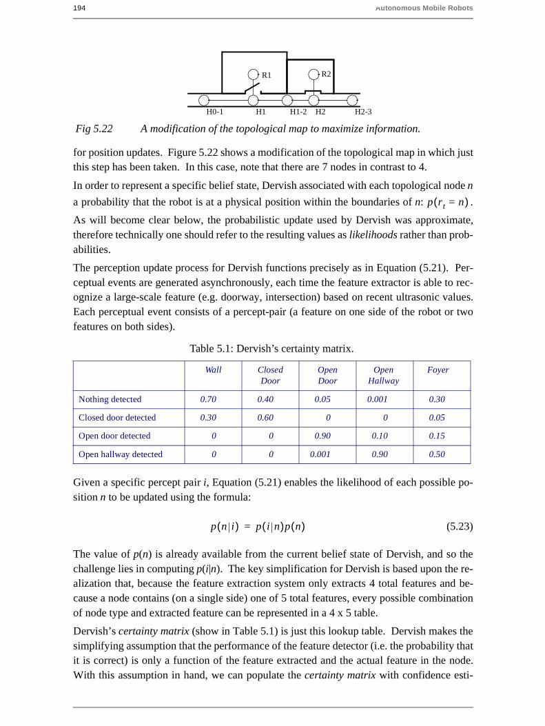
194 Autonomous Mobile Robots
for position updates. Figure 5.22 shows a modification of the topological map in which justthis step has been taken. In this case, note that there are 7 nodes in contrast to 4.
In order to represent a specific belief state, Dervish associated with each topological node n
a probability that the robot is at a physical position within the boundaries of n: .
As will become clear below, the probabilistic update used by Dervish was approximate,therefore technically one should refer to the resulting values as likelihoods rather than prob-abilities.
The perception update process for Dervish functions precisely as in Equation (5.21). Per-ceptual events are generated asynchronously, each time the feature extractor is able to rec-ognize a large-scale feature (e.g. doorway, intersection) based on recent ultrasonic values.Each perceptual event consists of a percept-pair (a feature on one side of the robot or twofeatures on both sides).
Given a specific percept pair i, Equation (5.21) enables the likelihood of each possible po-sition n to be updated using the formula:
(5.23)
The value of p(n) is already available from the current belief state of Dervish, and so thechallenge lies in computing p(i|n). The key simplification for Dervish is based upon the re-alization that, because the feature extraction system only extracts 4 total features and be-cause a node contains (on a single side) one of 5 total features, every possible combinationof node type and extracted feature can be represented in a 4 x 5 table.
Dervish’s certainty matrix (show in Table 5.1) is just this lookup table. Dervish makes thesimplifying assumption that the performance of the feature detector (i.e. the probability thatit is correct) is only a function of the feature extracted and the actual feature in the node.With this assumption in hand, we can populate the certainty matrix with confidence esti-
Table 5.1: Dervish’s certainty matrix.
Wall ClosedDoor
OpenDoor
OpenHallway
Foyer
Nothing detected 0.70 0.40 0.05 0.001 0.30
Closed door detected 0.30 0.60 0 0 0.05
Open door detected 0 0 0.90 0.10 0.15
Open hallway detected 0 0 0.001 0.90 0.50
Fig 5.22 A modification of the topological map to maximize information.
R1 R2
H1 H2H0-1 H1-2 H2-3
p rt n=( )
p n i( ) p i n( )p n( )=
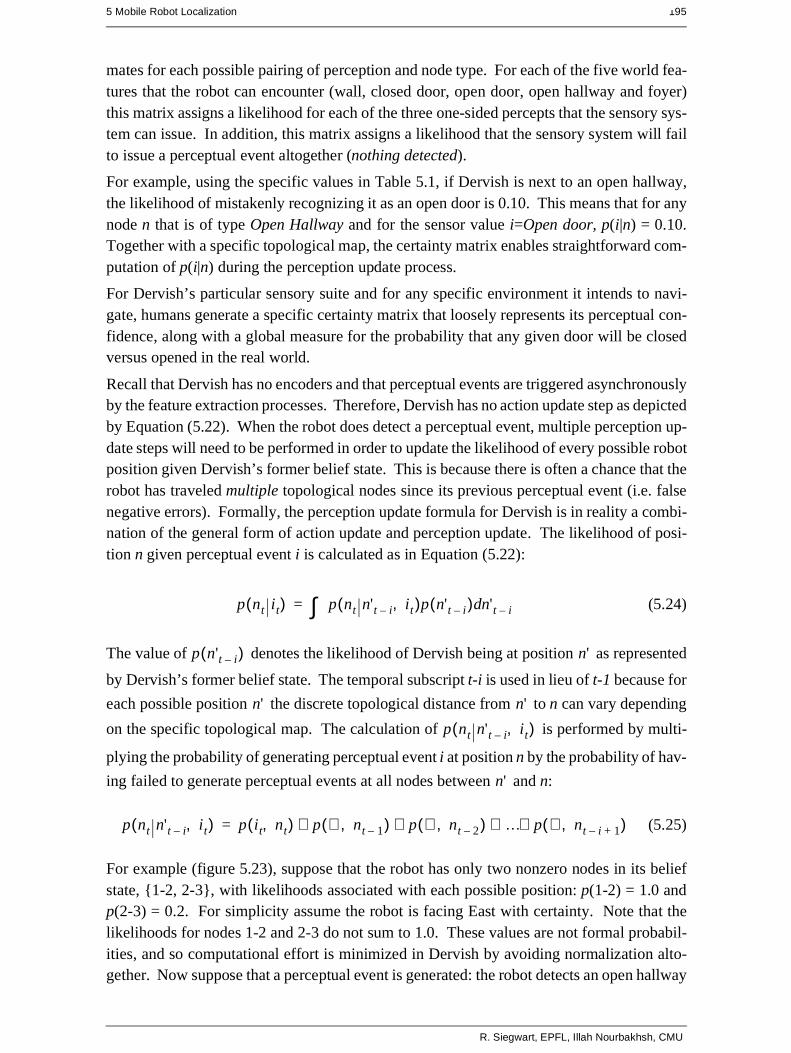
5 Mobile Robot Localization 195
mates for each possible pairing of perception and node type. For each of the five world fea-tures that the robot can encounter (wall, closed door, open door, open hallway and foyer)this matrix assigns a likelihood for each of the three one-sided percepts that the sensory sys-tem can issue. In addition, this matrix assigns a likelihood that the sensory system will failto issue a perceptual event altogether (nothing detected).
For example, using the specific values in Table 5.1, if Dervish is next to an open hallway,the likelihood of mistakenly recognizing it as an open door is 0.10. This means that for anynode n that is of type Open Hallway and for the sensor value i=Open door, p(i|n) = 0.10.Together with a specific topological map, the certainty matrix enables straightforward com-putation of p(i|n) during the perception update process.
For Dervish’s particular sensory suite and for any specific environment it intends to navi-gate, humans generate a specific certainty matrix that loosely represents its perceptual con-fidence, along with a global measure for the probability that any given door will be closedversus opened in the real world.
Recall that Dervish has no encoders and that perceptual events are triggered asynchronouslyby the feature extraction processes. Therefore, Dervish has no action update step as depictedby Equation (5.22). When the robot does detect a perceptual event, multiple perception up-date steps will need to be performed in order to update the likelihood of every possible robotposition given Dervish’s former belief state. This is because there is often a chance that therobot has traveled multiple topological nodes since its previous perceptual event (i.e. falsenegative errors). Formally, the perception update formula for Dervish is in reality a combi-nation of the general form of action update and perception update. The likelihood of posi-tion n given perceptual event i is calculated as in Equation (5.22):
(5.24)
The value of denotes the likelihood of Dervish being at position as represented
by Dervish’s former belief state. The temporal subscript t-i is used in lieu of t-1 because for
each possible position the discrete topological distance from to n can vary depending
on the specific topological map. The calculation of is performed by multi-
plying the probability of generating perceptual event i at position n by the probability of hav-
ing failed to generate perceptual events at all nodes between and n:
(5.25)
For example (figure 5.23), suppose that the robot has only two nonzero nodes in its beliefstate, {1-2, 2-3}, with likelihoods associated with each possible position: p(1-2) = 1.0 andp(2-3) = 0.2. For simplicity assume the robot is facing East with certainty. Note that thelikelihoods for nodes 1-2 and 2-3 do not sum to 1.0. These values are not formal probabil-ities, and so computational effort is minimized in Dervish by avoiding normalization alto-gether. Now suppose that a perceptual event is generated: the robot detects an open hallway
p nt it( ) p nt n't i– it,( )p n't i–( ) n't i–d∫=
p n't i–( ) n'
n' n'
p nt n't i– it,( )
n'
p nt n't i– it,( ) p it nt,( ) p ∅ nt 1–,( ) p ∅ nt 2–,( ) … p ∅ nt i– 1+,( )⋅ ⋅ ⋅ ⋅=
R. Siegwart, EPFL, Illah Nourbakhsh, CMU
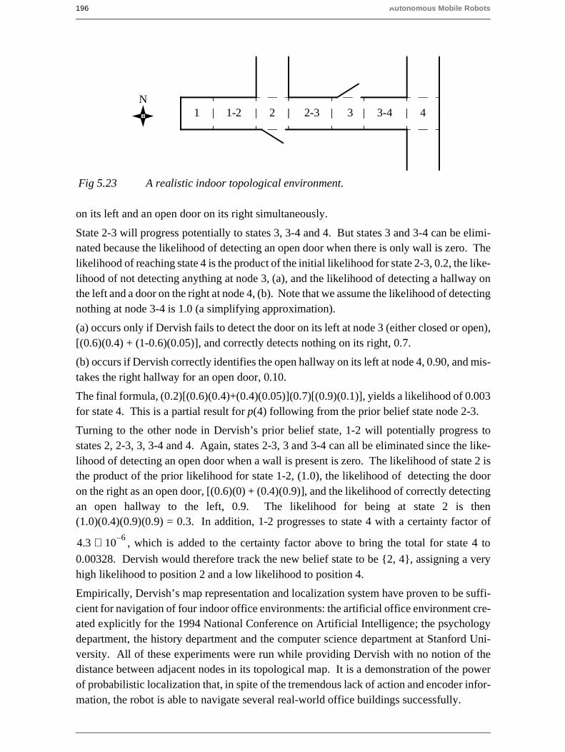
196 Autonomous Mobile Robots
on its left and an open door on its right simultaneously.
State 2-3 will progress potentially to states 3, 3-4 and 4. But states 3 and 3-4 can be elimi-nated because the likelihood of detecting an open door when there is only wall is zero. Thelikelihood of reaching state 4 is the product of the initial likelihood for state 2-3, 0.2, the like-lihood of not detecting anything at node 3, (a), and the likelihood of detecting a hallway onthe left and a door on the right at node 4, (b). Note that we assume the likelihood of detectingnothing at node 3-4 is 1.0 (a simplifying approximation).
(a) occurs only if Dervish fails to detect the door on its left at node 3 (either closed or open),[(0.6)(0.4) + (1-0.6)(0.05)], and correctly detects nothing on its right, 0.7.
(b) occurs if Dervish correctly identifies the open hallway on its left at node 4, 0.90, and mis-takes the right hallway for an open door, 0.10.
The final formula, (0.2)[(0.6)(0.4)+(0.4)(0.05)](0.7)[(0.9)(0.1)], yields a likelihood of 0.003for state 4. This is a partial result for p(4) following from the prior belief state node 2-3.
Turning to the other node in Dervish’s prior belief state, 1-2 will potentially progress tostates 2, 2-3, 3, 3-4 and 4. Again, states 2-3, 3 and 3-4 can all be eliminated since the like-lihood of detecting an open door when a wall is present is zero. The likelihood of state 2 isthe product of the prior likelihood for state 1-2, (1.0), the likelihood of detecting the dooron the right as an open door, [(0.6)(0) + (0.4)(0.9)], and the likelihood of correctly detectingan open hallway to the left, 0.9. The likelihood for being at state 2 is then(1.0)(0.4)(0.9)(0.9) = 0.3. In addition, 1-2 progresses to state 4 with a certainty factor of
, which is added to the certainty factor above to bring the total for state 4 to
0.00328. Dervish would therefore track the new belief state to be {2, 4}, assigning a veryhigh likelihood to position 2 and a low likelihood to position 4.
Empirically, Dervish’s map representation and localization system have proven to be suffi-cient for navigation of four indoor office environments: the artificial office environment cre-ated explicitly for the 1994 National Conference on Artificial Intelligence; the psychologydepartment, the history department and the computer science department at Stanford Uni-versity. All of these experiments were run while providing Dervish with no notion of thedistance between adjacent nodes in its topological map. It is a demonstration of the powerof probabilistic localization that, in spite of the tremendous lack of action and encoder infor-mation, the robot is able to navigate several real-world office buildings successfully.
Fig 5.23 A realistic indoor topological environment.
1 1-2 2 2-3 3 3-4 4N
4.3 106–⋅
5 Mobile Robot Localization 197
One open question remains with respect to Dervish’s localization system. Dervish was notjust a localizer but also a navigator. As with all multiple hypothesis systems, one must askthe question, how does the robot decide how to move, given that it has multiple possible ro-bot positions in its representation? The technique employed by Dervish is a most commontechnique in the mobile robotics field: plan the robot’s actions by assuming that the robot’sactual position is its most likely node in the belief state. Generally, the most likely positionis a good measure of the robot’s actual world position. However, this technique has short-comings when the highest and second highest most likely positions have similar values. Inthe case of Dervish, it nonetheless goes with the highest likelihood position at all times, saveat one critical juncture. The robot’s goal is to enter a target room and remain there. There-fore, from the point of view of its goal, it is critical that it finish navigating only when therobot has strong confidence in being at the correct final location. In this particular case, Der-vish’s execution module refuses to enter a room if the gap between the most likely positionand the second likeliest position is below a preset threshold. In such a case, Dervish willactively plan a path that causes it to move further down the hallway in an attempt to collectmore sensor data and thereby increase the relative likelihood of one position in the beliefstate.
Although computationally unattractive, one can go further, imagining a planning system forrobots such as Dervish for which one specifies a goal belief state rather than a goal position.The robot can then reason and plan in order to achieve a goal confidence level, thus explic-itly taking into account not only robot position but also the measured likelihood of each po-sition. An example of just such a procedure is the Sensory Uncertainty Field of Latombe[90], in which the robot must find a trajectory that reaches its goal while maximizing its lo-calization confidence enroute.
R. Siegwart, EPFL, Illah Nourbakhsh, CMU
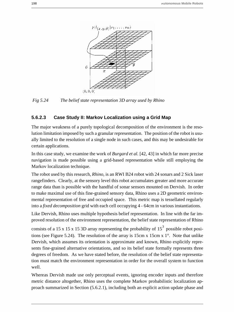
198 Autonomous Mobile Robots
5.6.2.3 Case Study II: Markov Localization using a Grid Map
The major weakness of a purely topological decomposition of the environment is the reso-lution limitation imposed by such a granular representation. The position of the robot is usu-ally limited to the resolution of a single node in such cases, and this may be undesirable forcertain applications.
In this case study, we examine the work of Burgard et al. [42, 43] in which far more precisenavigation is made possible using a grid-based representation while still employing theMarkov localization technique.
The robot used by this research, Rhino, is an RWI B24 robot with 24 sonars and 2 Sick laserrangefinders. Clearly, at the sensory level this robot accumulates greater and more accuraterange data than is possible with the handful of sonar sensors mounted on Dervish. In orderto make maximal use of this fine-grained sensory data, Rhino uses a 2D geometric environ-mental representation of free and occupied space. This metric map is tessellated regularlyinto a fixed decomposition grid with each cell occupying 4 - 64cm in various instantiations.
Like Dervish, Rhino uses multiple hypothesis belief representation. In line with the far im-proved resolution of the environment representation, the belief state representation of Rhino
consists of a 15 x 15 x 15 3D array representing the probability of possible robot posi-
tions (see Figure 5.24). The resolution of the array is 15cm x 15cm x 1°. Note that unlikeDervish, which assumes its orientation is approximate and known, Rhino explicitly repre-sents fine-grained alternative orientations, and so its belief state formally represents threedegrees of freedom. As we have stated before, the resolution of the belief state representa-tion must match the environment representation in order for the overall system to functionwell.
Whereas Dervish made use only perceptual events, ignoring encoder inputs and thereforemetric distance altogether, Rhino uses the complete Markov probabilistic localization ap-proach summarized in Section (5.6.2.1), including both an explicit action update phase and
153
Fig 5.24 The belief state representation 3D array used by Rhino

5 Mobile Robot Localization 199
a perception update phase at every cycle.
The discrete Markov chain version of action update is performed because of the tessellatedrepresentation of position. Given encoder measurements o at time t, each updated positionprobability in the belief state is expressed as a sum over previous possible positions and themotion model:
(5.26)
Note that Equation (5.26) is simply a discrete version of Equation (5.22). The specific mo-tion model used by Rhino represents the result of motion as a Gaussian that is bounded (i.e.the tails of the distribution are finite). Rhino’s kinematic configuration is a 3-wheel syn-chro-drive rather than a differential drive robot. Nevertheless, the error ellipses depicted inFigures (5.4) and (5.5) are similar to the Gaussian bounds that result from Rhino’s motionmodel.
The perception model follows Bayes formula precisely as in Equation (5.21). Given a rangeperception i the probability of the robot being at each location l is updated as follows:
(5.27)
Note that a denominator is used by Rhino, although the denominator is constant for varyingvalues of l. This denominator acts as a normalizer to ensure that the probability measures inthe belief state continue to sum to 1.
The critical challenge is, of course, the calculation of p(i|l). In the case of Dervish, the num-ber of possible values for i and l were so small that a simple table could suffice. However,with the fine-grained metric representation of Rhino, the number of possible sensor readingsand environmental geometric contexts is extremely large. Thus, Rhino computes p(i|l) di-rectly using a model of the robot’s sensor behavior, its position l and the local environmentalmetric map around l.
The sensor model must calculate the probability of a specific perceptual measurement giventhat its likelihood is justified by known errors of the sonar or laser rangefinder sensors.Three key assumptions are used to construct this sensor model:
1 If an object in the metric map is detected by a range sensor, the measurement errorcan be described with a distribution that has a mean at the correct reading.
2 There should always be a nonzero chance that a range sensor will read any measure-ment value, even if this measurement disagrees sharply with the environmental ge-ometry.
3 In contrast to the generic error described in #2, there is a specific failure mode inranging sensors whereby the signal is absorbed or coherently reflected, causing thesensor’s range measurement to be maximal. Therefore, there is a local peak in theprobability density distribution at the maximal reading of a range sensor.
P lt ot( ) P lt l't 1– ot,( ) p l't 1–( )⋅l'
∑=
p l i( )p i l( )p l( )
p i( )------------------------=
R. Siegwart, EPFL, Illah Nourbakhsh, CMU
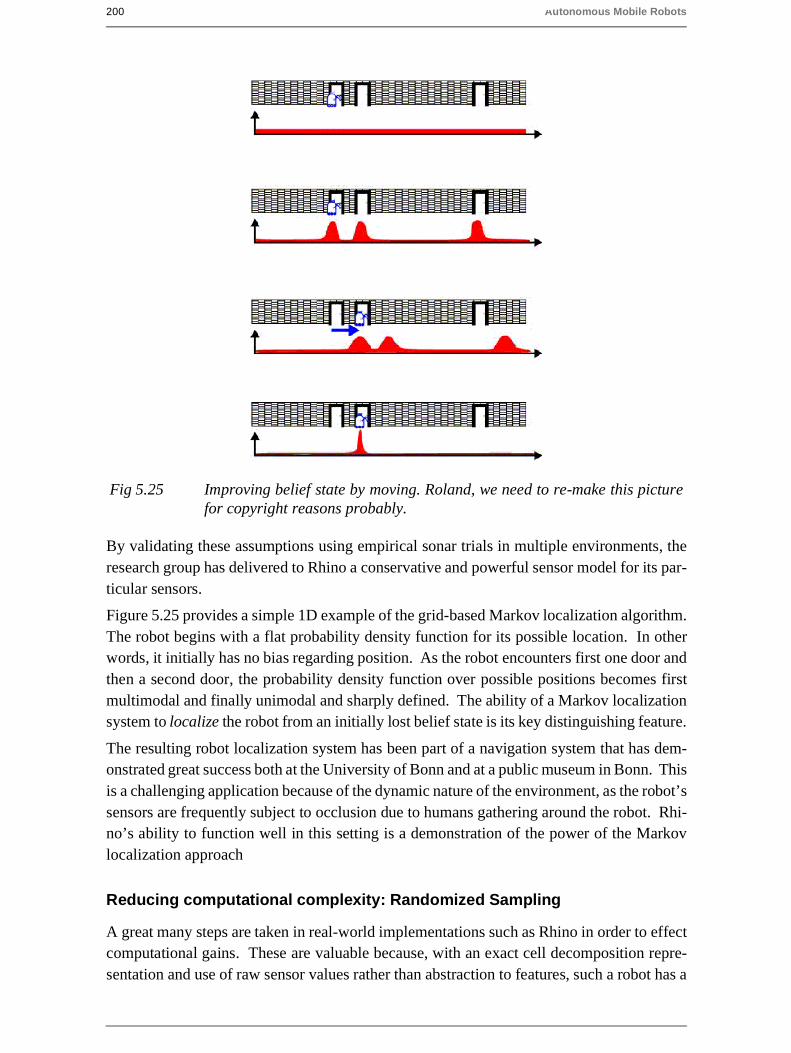
200 Autonomous Mobile Robots
By validating these assumptions using empirical sonar trials in multiple environments, theresearch group has delivered to Rhino a conservative and powerful sensor model for its par-ticular sensors.
Figure 5.25 provides a simple 1D example of the grid-based Markov localization algorithm.The robot begins with a flat probability density function for its possible location. In otherwords, it initially has no bias regarding position. As the robot encounters first one door andthen a second door, the probability density function over possible positions becomes firstmultimodal and finally unimodal and sharply defined. The ability of a Markov localizationsystem to localize the robot from an initially lost belief state is its key distinguishing feature.
The resulting robot localization system has been part of a navigation system that has dem-onstrated great success both at the University of Bonn and at a public museum in Bonn. Thisis a challenging application because of the dynamic nature of the environment, as the robot’ssensors are frequently subject to occlusion due to humans gathering around the robot. Rhi-no’s ability to function well in this setting is a demonstration of the power of the Markovlocalization approach
Reducing computational complexity: Randomized Sampling
A great many steps are taken in real-world implementations such as Rhino in order to effectcomputational gains. These are valuable because, with an exact cell decomposition repre-sentation and use of raw sensor values rather than abstraction to features, such a robot has a
Fig 5.25 Improving belief state by moving. Roland, we need to re-make this picturefor copyright reasons probably.

5 Mobile Robot Localization 201
massive computational effort associated with each perceptual update.
One class of techniques deserves mention because it can significantly reduce the computa-tional overhead of techniques that employ fixed-cell decomposition representations. Thebasic idea, which we call randomized sampling is known alternatively as Particle filter al-gorithms, Condensation algorithms and Monte Carlo algorithms [ROLAND, reference theThrun et al. paper on "Robust Monte Carlo" in my text file].
Irrespective of the specific technique, the basic algorithm is the same in all these cases. In-stead of representing every possibe robot position by representing the complete and correctbelief state, an approximate belief state is constructed by representing only a subset of thecomplete set of possible locations that should be considered.
For example, consider a robot with a complete belief state of 10,000 possible locations attime t. Instead of tracking and updating all 10,000 possible locations based on a new sensormeasurement, the robot can select only 10% of the stored locations and update only thoselocations. By weighting this sampling process with the probability values of the locations,one can bias the system to generate more samples at local peaks in the probability densityfunction. So, the resulting 1,000 locations will be concentrated primarily at the highestprobability locations. This biasing is desirable, but only to a point.
We also wish to ensure that some less likely locations are tracked, as otherwise, if the robotdoes indeed receive unlikely sensor measurements, it will fail to localize. This randomiza-tion of the sampling process can be performed by adding additional samples from a flat dis-tribution for example. Further enhancements of these randomized methods enable thenumber of statistical samples to be varied on-the-fly, based for instance on the ongoing lo-calization confidence of the system. This further reduces the number of samples requiredon average while guaranteeing that a large number of samples will be used when necessary[ROLAND, reference the Fox NIPS article on KLD-Sampling Adaptive Particle Filters]
These sampling techniques have resulted in robots that function indistinguishably as com-pared to their full belief state set ancestors, yet use computationally a fraction of the resourc-es. Of course, such sampling has a penalty: completeness. The probabilistically completenature of Markov localization is violated by these sampling approaches because the robot isfailing to update all the nonzero probability locations, and thus there is a danger that the ro-bot, due to an unlikely but correct sensor reading, could become truly lost. Of course, re-covery from a lost state is feasible just as with all Markov localization techniques.
R. Siegwart, EPFL, Illah Nourbakhsh, CMU
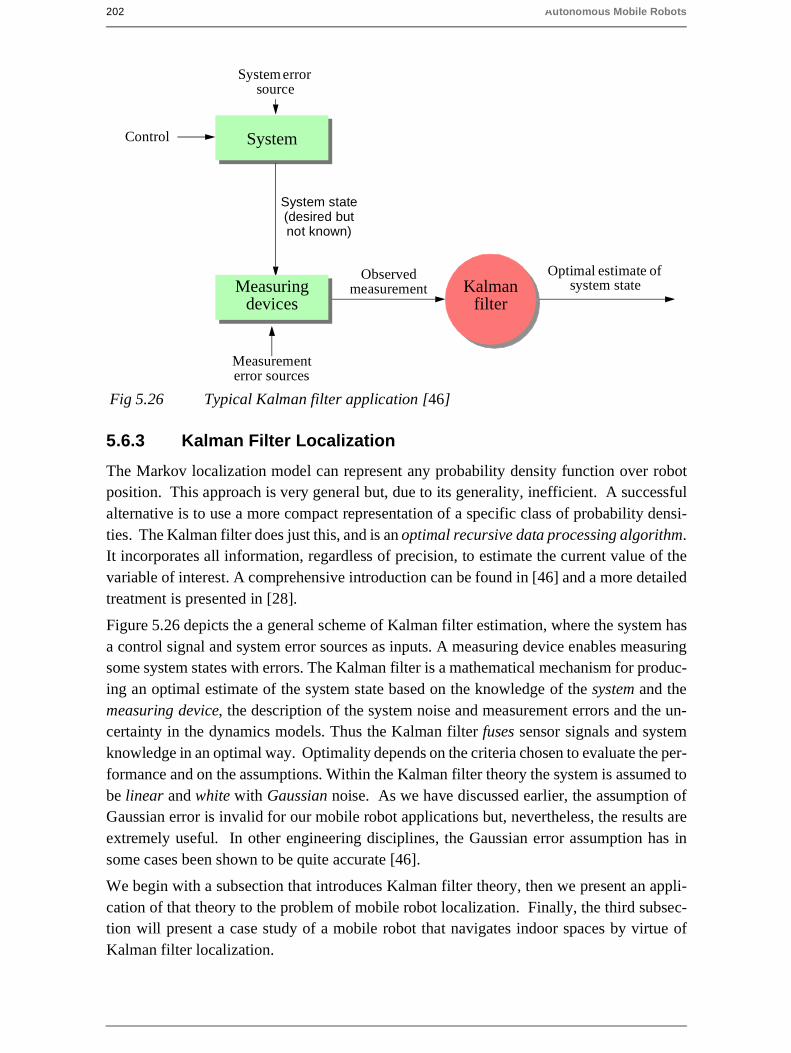
202 Autonomous Mobile Robots
5.6.3 Kalman Filter Localization
The Markov localization model can represent any probability density function over robotposition. This approach is very general but, due to its generality, inefficient. A successfulalternative is to use a more compact representation of a specific class of probability densi-ties. The Kalman filter does just this, and is an optimal recursive data processing algorithm.It incorporates all information, regardless of precision, to estimate the current value of thevariable of interest. A comprehensive introduction can be found in [46] and a more detailedtreatment is presented in [28].
Figure 5.26 depicts the a general scheme of Kalman filter estimation, where the system hasa control signal and system error sources as inputs. A measuring device enables measuringsome system states with errors. The Kalman filter is a mathematical mechanism for produc-ing an optimal estimate of the system state based on the knowledge of the system and themeasuring device, the description of the system noise and measurement errors and the un-certainty in the dynamics models. Thus the Kalman filter fuses sensor signals and systemknowledge in an optimal way. Optimality depends on the criteria chosen to evaluate the per-formance and on the assumptions. Within the Kalman filter theory the system is assumed tobe linear and white with Gaussian noise. As we have discussed earlier, the assumption ofGaussian error is invalid for our mobile robot applications but, nevertheless, the results areextremely useful. In other engineering disciplines, the Gaussian error assumption has insome cases been shown to be quite accurate [46].
We begin with a subsection that introduces Kalman filter theory, then we present an appli-cation of that theory to the problem of mobile robot localization. Finally, the third subsec-tion will present a case study of a mobile robot that navigates indoor spaces by virtue ofKalman filter localization.
System
Fig 5.26 Typical Kalman filter application [46]
System state(desired butnot known)
Control
Measuringdevices
System errorsource
Measurementerror sources
Observedmeasurement
Optimal estimate ofsystem stateKalman
filter
5 Mobile Robot Localization 203
5.6.3.1 Introduction to Kalman Filter Theory
The basic Kalman filter method allows multiple measurements to be incorporated optimallyinto a single estimate of state. In demonstrating this, first we make the simplifying assump-tion that the state does not change (e.g. the robot does not move) between the acquisition ofthe first and second measurement. After presenting this static case, we can introduce dy-namic prediction readily.
Static Estimation
Assume we have taken two measurements, one with an ultrasonic range sensor at time k andone with a more precise laser range sensor at time k+1. Based on each measurement we areable to estimate the robot’s position. Such an estimate derived from the first sensor mea-surements is q1 and the estimate of position based on the second measurement is q2. Since
we know that each measurement can be inaccurate, we wish to modulate these position es-timates based on the measurement error expected from each sensor. Suppose that we use
two variances and to predict the error associated with each measurement. We will,
of course, assume a unimodal error distribution throughout the remainder of the Kalman fil-ter approach, yielding the two robot position estimates:
with variance (5.28)
with variance . (5.29)
So we have two measurements available to estimate the robots position. The question is,
how do we fuse (combine) these data to get the best estimate for the robot position?
We are assuming that there was no robot motion between time k and time k+1, and thereforewe can directly apply the same weighted least square technique of Equation 4.61 in Section4.3.1.1. Thus we write:
(5.30)
with wi being the weight of measurement i. To find the minimum error we set the derivative
of S equal to zero.
(5.31)
σ12 σ2
2
q1 q1= σ12
q2 q2= σ22
q
S wi q qi–( )2
i 1=
n
∑=
S∂q∂
-----q∂∂
wi q qi–( )2
i 1=
n
∑ 2 wi q qi–( )i 1=
n
∑ 0= = =
R. Siegwart, EPFL, Illah Nourbakhsh, CMU
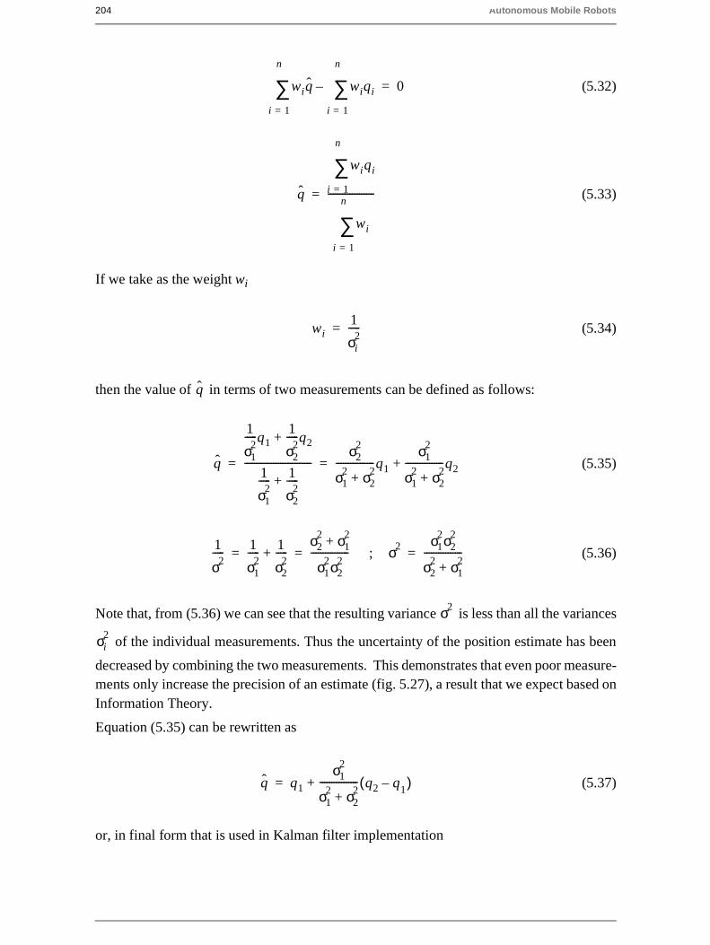
204 Autonomous Mobile Robots
(5.32)
(5.33)
If we take as the weight wi
(5.34)
then the value of in terms of two measurements can be defined as follows:
(5.35)
; (5.36)
Note that, from (5.36) we can see that the resulting variance is less than all the variances
of the individual measurements. Thus the uncertainty of the position estimate has been
decreased by combining the two measurements. This demonstrates that even poor measure-ments only increase the precision of an estimate (fig. 5.27), a result that we expect based onInformation Theory.
Equation (5.35) can be rewritten as
(5.37)
or, in final form that is used in Kalman filter implementation
wiq
i 1=
n
∑ wiqi
i 1=
n
∑– 0=
q
wiqi
i 1=
n
∑
wi
i 1=
n
∑-------------------=
wi1
σi2
-----=
q
q
1
σ12
-----q11
σ22
-----q2+
1
σ12
----- 1
σ22
-----+----------------------------
σ22
σ12 σ2
2+
----------------q1
σ12
σ12 σ2
2+
----------------q2+= =
1
σ2----- 1
σ12
----- 1
σ22
-----+σ2
2 σ12
+
σ12σ2
2----------------= = σ2
σ12σ2
2
σ22 σ1
2+
----------------=
σ2
σi2
q q1
σ12
σ12 σ2
2+
---------------- q2 q– 1( )+=
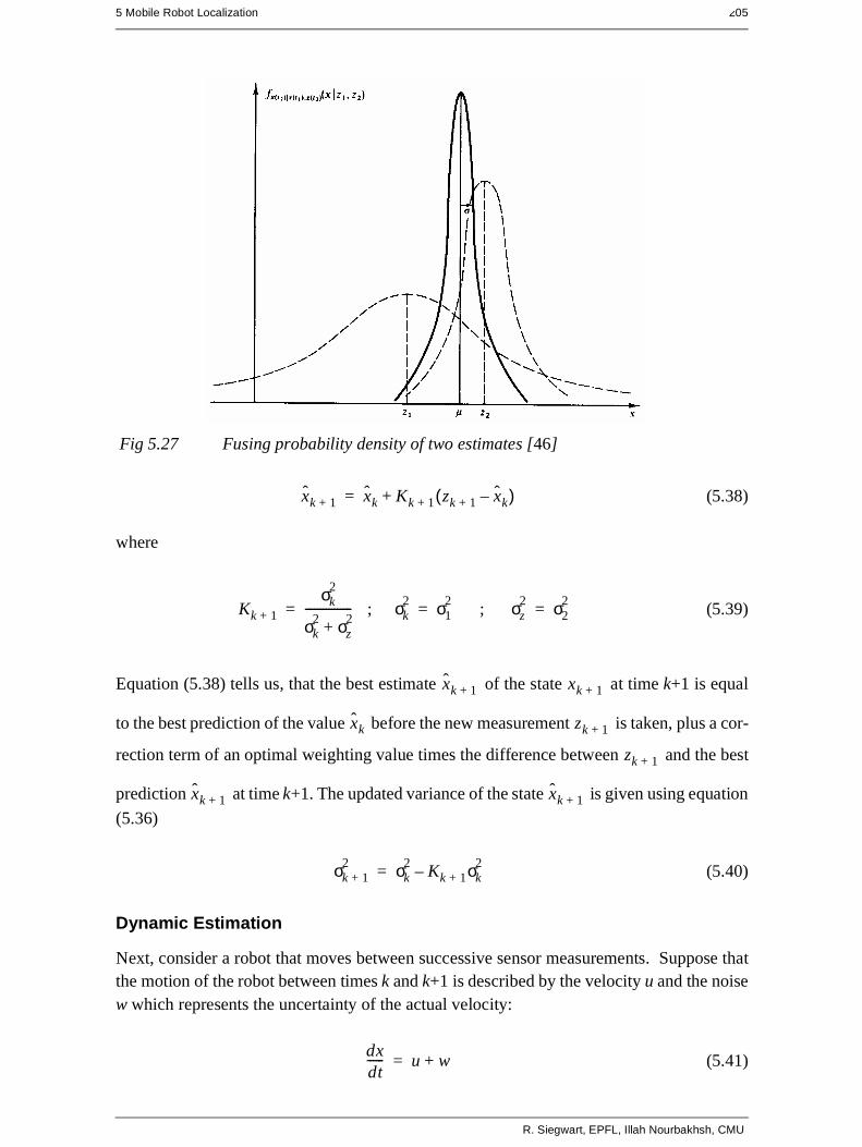
5 Mobile Robot Localization 205
(5.38)
where
; ; (5.39)
Equation (5.38) tells us, that the best estimate of the state at time k+1 is equal
to the best prediction of the value before the new measurement is taken, plus a cor-
rection term of an optimal weighting value times the difference between and the best
prediction at time k+1. The updated variance of the state is given using equation
(5.36)
(5.40)
Dynamic Estimation
Next, consider a robot that moves between successive sensor measurements. Suppose thatthe motion of the robot between times k and k+1 is described by the velocity u and the noisew which represents the uncertainty of the actual velocity:
(5.41)
Fig 5.27 Fusing probability density of two estimates [46]
xk 1+ xk Kk 1+ zk 1+ xk–( )+=
Kk 1+
σk2
σk2 σz
2+
----------------= σk2 σ1
2= σz
2 σ22
=
xk 1+ xk 1+
xk zk 1+
zk 1+
xk 1+ xk 1+
σk 1+2 σk
2Kk 1+ σk
2–=
dxdt------ u w+=
R. Siegwart, EPFL, Illah Nourbakhsh, CMU
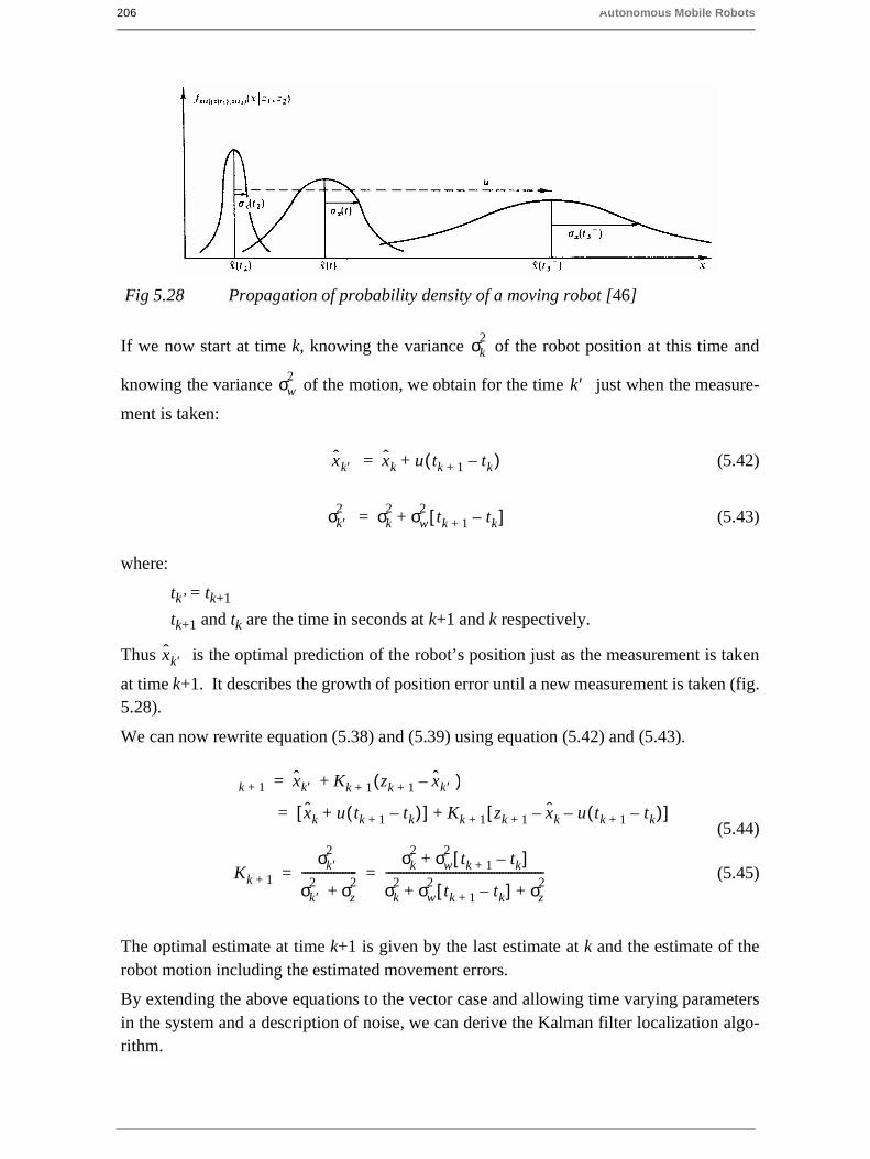
206 Autonomous Mobile Robots
If we now start at time k, knowing the variance of the robot position at this time and
knowing the variance of the motion, we obtain for the time just when the measure-
ment is taken:
(5.42)
(5.43)
where:
tk’ = tk+1
tk+1 and tk are the time in seconds at k+1 and k respectively.
Thus is the optimal prediction of the robot’s position just as the measurement is taken
at time k+1. It describes the growth of position error until a new measurement is taken (fig.5.28).
We can now rewrite equation (5.38) and (5.39) using equation (5.42) and (5.43).
(5.44)
(5.45)
The optimal estimate at time k+1 is given by the last estimate at k and the estimate of therobot motion including the estimated movement errors.
By extending the above equations to the vector case and allowing time varying parametersin the system and a description of noise, we can derive the Kalman filter localization algo-rithm.
σk2
σw2
k′
xk′ xk u tk 1+ tk–( )+=
σk′2 σk
2 σw2
tk 1+ tk–[ ]+=
xk ′
Fig 5.28 Propagation of probability density of a moving robot [46]
k 1+ xk′ Kk 1+ zk 1+ xk ′–( )+=
xk 1+ xk u tk 1+ tk–( )+[ ] Kk 1+ zk 1+ xk– u tk 1+ tk–( )–[ ]+=
Kk 1+
σk ′2
σk ′2 σz
2+
-------------------σk
2 σw2
tk 1+ tk–[ ]+
σk2 σw
2tk 1+ tk–[ ] σz
2+ +
------------------------------------------------------= =
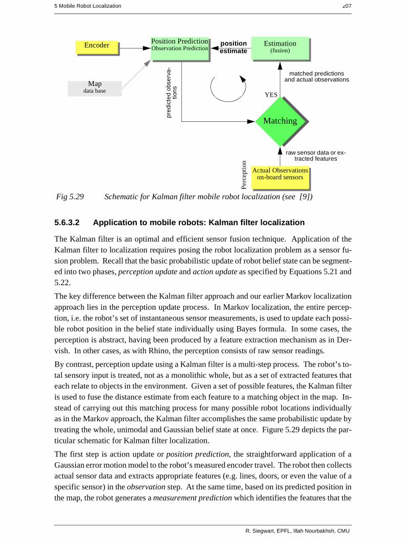
5 Mobile Robot Localization 207
5.6.3.2 Application to mobile robots: Kalman filter localization
The Kalman filter is an optimal and efficient sensor fusion technique. Application of theKalman filter to localization requires posing the robot localization problem as a sensor fu-sion problem. Recall that the basic probabilistic update of robot belief state can be segment-ed into two phases, perception update and action update as specified by Equations 5.21 and5.22.
The key difference between the Kalman filter approach and our earlier Markov localizationapproach lies in the perception update process. In Markov localization, the entire percep-tion, i.e. the robot’s set of instantaneous sensor measurements, is used to update each possi-ble robot position in the belief state individually using Bayes formula. In some cases, theperception is abstract, having been produced by a feature extraction mechanism as in Der-vish. In other cases, as with Rhino, the perception consists of raw sensor readings.
By contrast, perception update using a Kalman filter is a multi-step process. The robot’s to-tal sensory input is treated, not as a monolithic whole, but as a set of extracted features thateach relate to objects in the environment. Given a set of possible features, the Kalman filteris used to fuse the distance estimate from each feature to a matching object in the map. In-stead of carrying out this matching process for many possible robot locations individuallyas in the Markov approach, the Kalman filter accomplishes the same probabilistic update bytreating the whole, unimodal and Gaussian belief state at once. Figure 5.29 depicts the par-ticular schematic for Kalman filter localization.
The first step is action update or position prediction, the straightforward application of aGaussian error motion model to the robot’s measured encoder travel. The robot then collectsactual sensor data and extracts appropriate features (e.g. lines, doors, or even the value of aspecific sensor) in the observation step. At the same time, based on its predicted position inthe map, the robot generates a measurement prediction which identifies the features that the
Actual Observationson-board sensors
Mapdata base
Position PredictionObservation Prediction
Fig 5.29 Schematic for Kalman filter mobile robot localization (see [9])
Per
cept
ion
Matching
Estimation(fusion)
raw sensor data or ex-tracted features
pred
icte
dob
serv
a-tio
ns
positionestimate
matched predictionsand actual observations
YES
Encoder
R. Siegwart, EPFL, Illah Nourbakhsh, CMU

208 Autonomous Mobile Robots
robot expects to find and the positions of those features. In matching the robot identifies thebest pairings between the features actually extracted during observation and the expectedfeatures due to measurement prediction. Finally, the Kalman filter can fuse the informationprovided by all of these matches in order to update the robot belief state in estimation.
In the following sub-sections these five steps are described in greater detail. The presenta-tion is based on the work of Leonard and Durrant-Whyte [9 page 61-65].
1. Robot Position Prediction
The robot’s position at time step k+1 is predicted based on its old location (at time step k)
and its movement due to the control input :
(5.46)
For the differential drive robot, is derived in Equations (5.6) and (5.7) re-
spectively.
Knowing the plant and error model, we can also compute the variance associ-
ated with this prediction (see eq. (5.9) section 5.2.4):
(5.47)
This allows us to predict the robot’s position and its uncertainty after a movement specified
by the control input . Note that the belief state is assumed to be Gaussian, and so we
can characterize the believe state with just the two parameters and .
2. Observation
The second step it to obtain sensor measurements from the robot at time k+1. In
this presentation, we assume that the observation is the result of a feature extraction process
executed on the raw sensor data. Therefore, the observation consists of a set of single
observations extracted from various sensors. Formally each single observation can
represent an extracted features such as a line or door, or even a single, raw sensor value.
The parameters of the features are usually specified in the sensor frame and therefore in alocal reference frame of the robot. However, for matching we need to represent the obser-
vations and measurement predictions in the same frame . In our presentation we will
transform the measurement predictions from the global coordinate frame to the sensor frame
. This transformation is specified in the function discussed in the next paragraph.
u k( )
p k 1 k+( ) f p k k( ) u k( ),( )=
p k 1 k+( ) p'=
Σp k 1 k+( )
Σp k 1 k+( ) ∇ pf Σp k k( ) ∇ pfT ∇ uf Σu k( ) ∇ uf
T⋅⋅+⋅⋅=
u k( )p k 1 k+( ) Σp k 1 k+( )
Z k 1+( )
n0
zj k 1+( )
S{ }
S{ } hi

5 Mobile Robot Localization 209
3. Measurement Prediction
We use the predicted robot position and the map to generate multiple pre-
dicted feature observations . Each predicted feature has its position transformed into the
sensor frame:
(5.48)
We can define the measurement prediction as the set containing all predicted feature ob-
servations:
(5.49)
The predicted state estimate is used to compute the measurement Jacobian
for each prediction. As you will see in the example below, the function is mainly a coor-
dinate transformation between the world frame and the sensor frame.
4. Matching
At this point we have a set of actual, single observations, which are features in sensor space,and we also have a set of predicted features, also positioned in sensor space. The matchingstep has the purpose of identifying all of the single observations that match specific predict-ed features well enough to be used during the estimation process. In other words, we will,for a subset of the observations and a subset of the predicted features, find pairings that in-tuitively say "this observation is the robot’s measurement of this predicted feature based onthe map."
Formally, the goal of the matching procedure is to produce an assignment from observations
to the targets (stored in the map). For each measurement prediction for which
a corresponding observation is found we calculate the innovation . Innovation is
a measure of the difference between the predicted and observed measurements:
(5.50)
The innovation covariance can be found by applying the error propagation
law (section 4.2.3 equation (4.60)):
(5.51)
where represents the covariance (noise) of the measurement .
To determine the validity of the correspondence between measurement prediction and ob-servation, a validation gate has to be specified. A possible definition of the validation gateis the Mahalanobis distance:
p k 1 k+( ) M k( )
zt
ziˆ k 1+( ) hi zt p k 1+ k( ),( )=
nt
Z k 1+( ) ziˆ k 1+( ) 1 i nt≤ ≤( ){ }=
p k 1 k+( ) ∇ hi
hi
zj k 1+( ) zt
vij k 1+( )
vij k 1+( ) zj k 1+( ) zi k 1+( )–[ ]=vij k 1+( ) zj k 1+( ) hi zt p k 1+ k( ),( )–[ ]=
ΣIN ij, k 1+( )
ΣIN ij, k 1+( ) ∇ hi Σp k 1+ k( ) ∇ hiT ΣR i, k 1+( )+⋅⋅=
ΣR i, k 1+( ) zi k 1+( )
R. Siegwart, EPFL, Illah Nourbakhsh, CMU
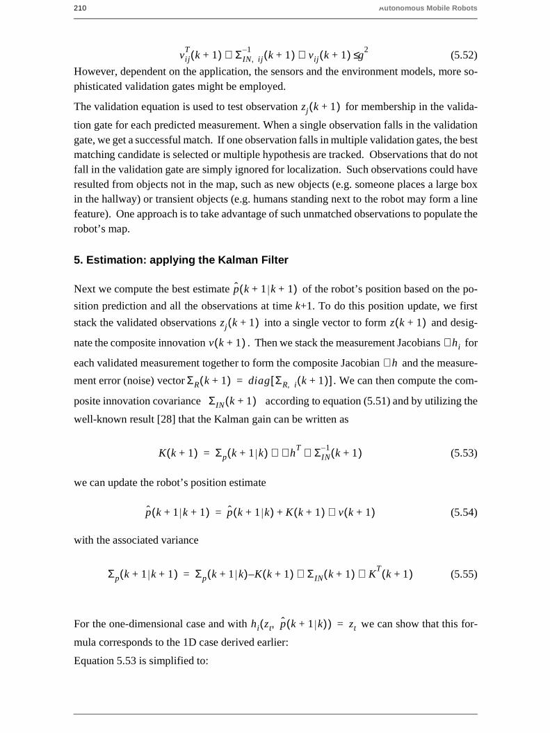
210 Autonomous Mobile Robots
(5.52)
However, dependent on the application, the sensors and the environment models, more so-phisticated validation gates might be employed.
The validation equation is used to test observation for membership in the valida-
tion gate for each predicted measurement. When a single observation falls in the validationgate, we get a successful match. If one observation falls in multiple validation gates, the bestmatching candidate is selected or multiple hypothesis are tracked. Observations that do notfall in the validation gate are simply ignored for localization. Such observations could haveresulted from objects not in the map, such as new objects (e.g. someone places a large boxin the hallway) or transient objects (e.g. humans standing next to the robot may form a linefeature). One approach is to take advantage of such unmatched observations to populate therobot’s map.
5. Estimation: applying the Kalman Filter
Next we compute the best estimate of the robot’s position based on the po-
sition prediction and all the observations at time k+1. To do this position update, we first
stack the validated observations into a single vector to form and desig-
nate the composite innovation . Then we stack the measurement Jacobians for
each validated measurement together to form the composite Jacobian and the measure-
ment error (noise) vector . We can then compute the com-
posite innovation covariance according to equation (5.51) and by utilizing the
well-known result [28] that the Kalman gain can be written as
(5.53)
we can update the robot’s position estimate
(5.54)
with the associated variance
(5.55)
For the one-dimensional case and with we can show that this for-
mula corresponds to the 1D case derived earlier:
Equation 5.53 is simplified to:
vijT
k 1+( ) ΣIN ij,1–
k 1+( ) vij k 1+( ) g2≤⋅⋅
zj k 1+( )
p k 1 k 1+ +( )
zj k 1+( ) z k 1+( )
v k 1+( ) hi∇
h∇ΣR k 1+( ) diag ΣR i, k 1+( )[ ]=
ΣIN k 1+( )
K k 1+( ) Σp k 1 k+( ) hT ΣIN
1–k 1+( )⋅∇⋅=
p k 1 k 1+ +( ) p k 1 k+( ) K k 1+( ) v k 1+( )⋅+=
Σp k 1 k 1+ +( ) Σp k 1 k+( ) K– k 1+( ) ΣIN k 1+( ) KT
k 1+( )⋅⋅=
hi zt p k 1+ k( ),( ) zt=

5 Mobile Robot Localization 211
(5.56)
corresponding to equation (5.45) and Equation 5.54 simplifies to:
(5.57)
corresponding to equation (5.44).
5.6.3.3 Case study: Kalman filter localization with line feature extraction
The Pygmalion robot at EPFL is a differential drive robot that uses a laser rangefinder as itsprimary sensor [39], [76]. In contrast to both Dervish and Rhino, the environmental repre-sentation of Pygmalion is continuous and abstract: the map consists of a set of infinite linesdescribing the environment. Pygmalion’s belief state is, of course, represented as a Gauss-ian distribution since this robot uses the Kalman filter localization algorithm. The value of
its mean position is represented to a high level of precision, enabling Pygmalion to local-
ize with very high precision when desired. Below, we present details for Pygmalion’s im-plementation of the five Kalman filter localization steps. For simplicity we assume that the
sensor frame is equal to the robot frame . If not specified all the vectors are rep-
resented in the world coordinate system .
1. Robot Position Prediction
At the time increment k the robot is at position and its best po-
sition estimate is . The control input drives the robot to the position
(fig. 5.30).
The robot position prediction at the time increment k+1 can be computed from the
previous estimate and the odometric integration of the movement. For the differen-
tial drive that Pygmalion has we can use the model (odometry) developed in section 5.2.4:
K k 1+( )σp
2k 1 k+( )
σIN2
k 1+( )---------------------------
σp2
k 1 k+( )
σp2
k 1+ k( ) σR2
k 1+( )+--------------------------------------------------------= =
k 1 k 1+ +( ) p k 1 k+( ) K k 1+( ) v k 1+( )⋅+=
k 1 k 1+ +( ) p k 1 k+( ) K k 1+( ) zj k 1+( ) hi zt p k 1+ k( ),( )–[ ]⋅+=
p k 1 k 1+ +( ) p k 1 k+( ) K k 1+( ) zj k 1+( ) zt–[ ]⋅+=
µ
S{ } R{ }W{ }
p k( ) x k( ) y k( ) θ k( )T
=
p k k( ) u k( ) p k 1+( )
p k 1+( )
p k k( )
R. Siegwart, EPFL, Illah Nourbakhsh, CMU

212 Autonomous Mobile Robots
(5.58)
with the updated covariance matrix
(5.59)
where
(5.60)
2. Observation
For line based localization, each single observation (i.e. a line feature) is extracted from the
raw laser rangefinder data and consists of the two line parameters , or , (fig.
4.36) respectively. For a rotating laser rangefinder, a representation in the polar coordinateframe is more appropriate and so we use this coordinate frame here:
(5.61)
x
y
Fig 5.30 Prediction of the robots position (magenta) based on its former position(blue) and the executed movement. The ellipses drawn around the robot po-sitions represent the uncertainties in the x,y direction (e.g. ). The uncer-
tainty of the orientation is not represented in the picture.
3σθ
t=k
t=k+1
p k( )x k( )y k( )θ k( )
=
p k 1+( )θ
W{ }
p k 1 k+( ) p k k( ) u k( )+ p k k( )
∆sr ∆sl+
2---------------------- θ
∆sr ∆– sl
2b-------------------+
cos
∆sr ∆sl+
2---------------------- θ
∆sr ∆– sl
2b-------------------+
sin
∆sr ∆– sl
b-------------------
+= =
k 1 k+( ) ∇ pf Σp k k( ) ∇ pfT ∇ uf Σu k( ) ∇ u⋅⋅+⋅⋅=
Σu cov ∆sr ∆sl,( )kr ∆sr 0
0 kl ∆sl
= =
β0 j, β1 j, αj rj
zj k 1+( )αj
rj
R
=
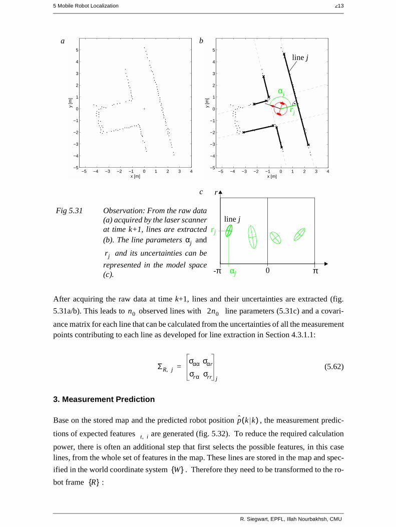
5 Mobile Robot Localization 213
After acquiring the raw data at time k+1, lines and their uncertainties are extracted (fig.
5.31a/b). This leads to observed lines with line parameters (5.31c) and a covari-
ance matrix for each line that can be calculated from the uncertainties of all the measurementpoints contributing to each line as developed for line extraction in Section 4.3.1.1:
(5.62)
3. Measurement Prediction
Base on the stored map and the predicted robot position , the measurement predic-
tions of expected features are generated (fig. 5.32). To reduce the required calculation
power, there is often an additional step that first selects the possible features, in this caselines, from the whole set of features in the map. These lines are stored in the map and spec-
ified in the world coordinate system . Therefore they need to be transformed to the ro-
bot frame :
Fig 5.31 Observation: From the raw data(a) acquired by the laser scannerat time k+1, lines are extracted(b). The line parameters and
and its uncertainties can be
represented in the model space(c).
αj
rj
−5 −4 −3 −2 −1 0 1 2 3 4−5
−4
−3
−2
−1
0
1
2
3
4
5
x [m]
y [m
]
−5 −4 −3 −2 −1 0 1 2 3 4−5
−4
−3
−2
−1
0
1
2
3
4
5
x [m]
y [m
]
αj
rj
line j
a b
αj
r
π-π
line j
0
rj
c
n0 2n0
ΣR j,σαα σαr
σrα σrr j
=
p k k( )
t i,
W{ }R{ }
R. Siegwart, EPFL, Illah Nourbakhsh, CMU

214 Autonomous Mobile Robots
(5.63)
According to figure (5.32), the transformation is given by
(5.64)
and its Jacobian by
(5.65)
The measurement prediction results in predicted lines represented in the robot coordinateframe (fig. 5.33). They are uncertain, because the prediction of robot position is uncertain.
4. Matching
For matching, we must find correspondence (or a pairing) between predicted and observedfeatures (fig. 5.34). In our case we take the Mahalanobis distance
(5.66)
x
y
Fig 5.32 Representation of the target position in the world coordinate frame
and robot coordinate frame .
W{ }R{ }
R{ }
p k 1+( )x k 1+( )y k 1+( )θ k 1+( ) )
=αR i
rR
i
θ k 1+( )
rW
i
W{ }αW
i
zt i,αt i,
rt i,
W
zR
t i,αt i,
rt i,
R
=→=
i k 1+( )αt i,
rt i,
R
= hi zt i, p k 1+ k( ),( )=
i k 1+( )αW
t i, θ k 1 k+( )W
–
rW
t i, x k 1 k+( )W αWt i,( )cos y k 1 k+( )W αW
t i,( )sin+( )–=
hi∇
hi∇
αt i,∂x∂
------------αt i,∂
y∂------------
αt i,∂
θ∂------------
rt i,∂x∂
-----------rt i,∂y∂
-----------rt i,∂
θ∂-----------
0 0 1–
αWt i,cos– αW
t i,sin– 0= =
ijT
k 1+( ) ΣIN ij,1–
k 1+( ) vij k 1+( ) g2≤⋅⋅
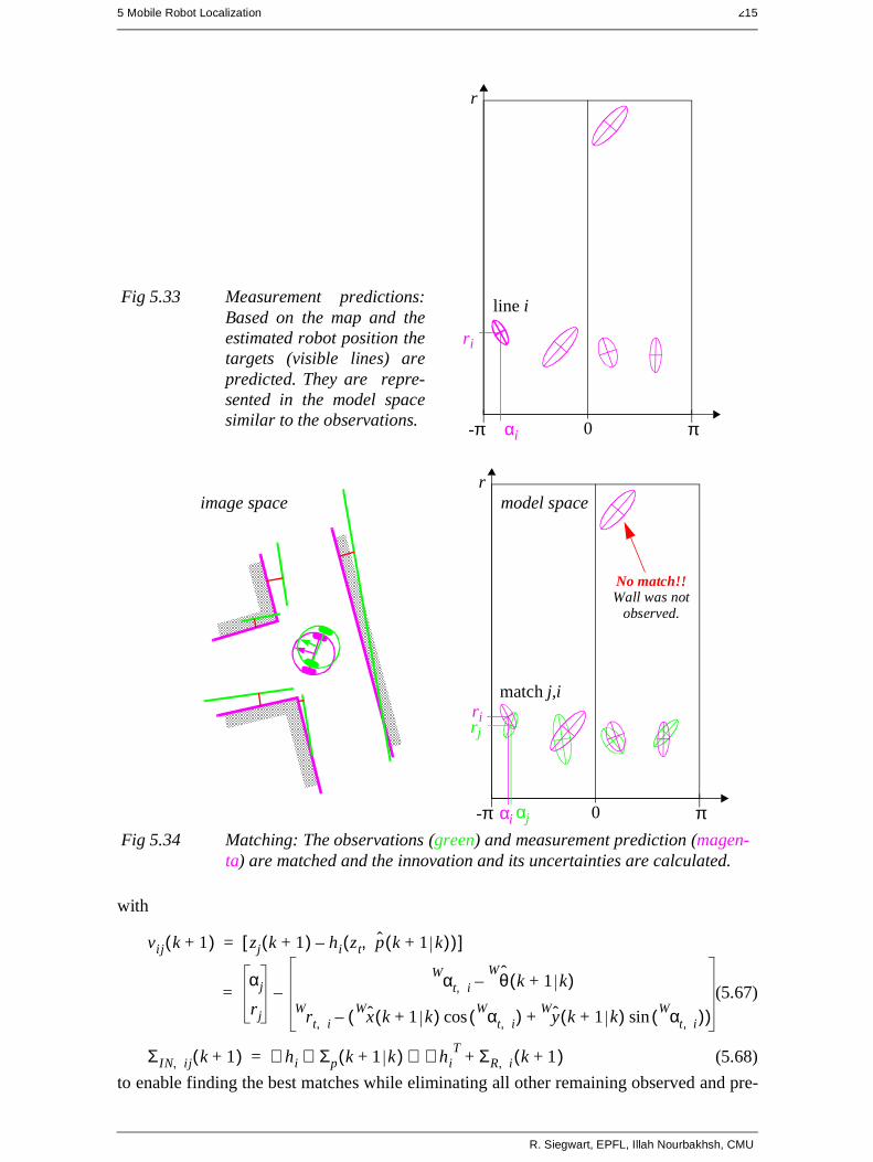
5 Mobile Robot Localization 215
with
(5.67)
(5.68)
to enable finding the best matches while eliminating all other remaining observed and pre-
Fig 5.33 Measurement predictions:Based on the map and theestimated robot position thetargets (visible lines) arepredicted. They are repre-sented in the model spacesimilar to the observations. αi
r
π-π
line i
0
ri
Fig 5.34 Matching: The observations (green) and measurement prediction (magen-ta) are matched and the innovation and its uncertainties are calculated.
αi
r
π-π
match j,i
0
ri
αj
rj
No match!!Wall was not
observed.
image space model space
vij k 1+( ) zj k 1+( ) hi zt p k 1+ k( ),( )–[ ]=
vij k 1–( )αj
rj
αWt i, θ k 1 k+( )
W–
rW
t i, x k 1 k+( )W αWt i,( )cos y k 1 k+( )W αW
t i,( )sin+( )––=
ΣIN ij, k 1+( ) ∇ hi Σp k 1+ k( ) ∇ hiT ΣR i, k 1+( )+⋅⋅=
R. Siegwart, EPFL, Illah Nourbakhsh, CMU
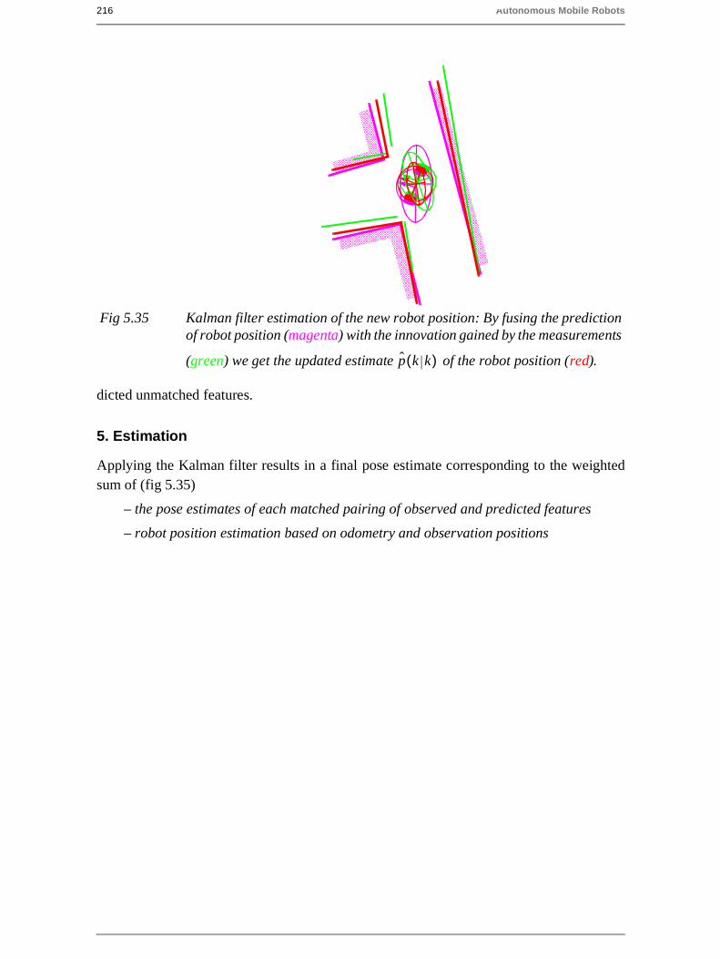
216 Autonomous Mobile Robots
dicted unmatched features.
5. Estimation
Applying the Kalman filter results in a final pose estimate corresponding to the weightedsum of (fig 5.35)
– the pose estimates of each matched pairing of observed and predicted features
– robot position estimation based on odometry and observation positions
Fig 5.35 Kalman filter estimation of the new robot position: By fusing the predictionof robot position (magenta) with the innovation gained by the measurements
(green) we get the updated estimate of the robot position (red).p k k( )
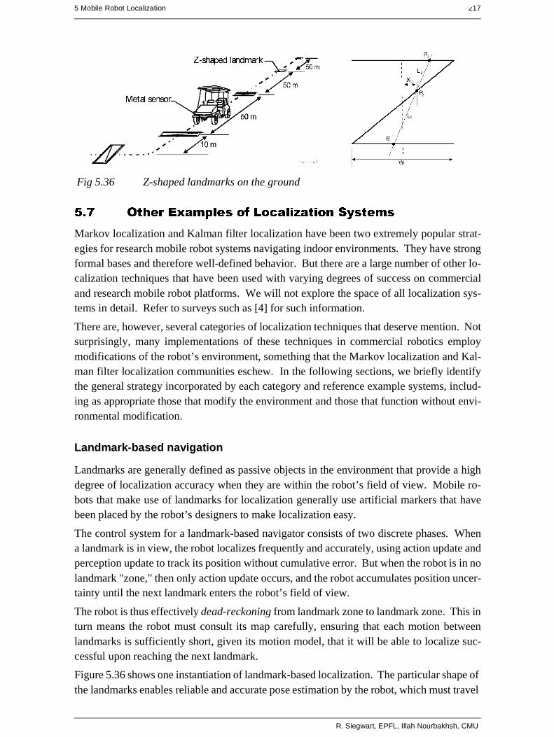
5 Mobile Robot Localization 217
5.7 Other Examples of Localization Systems
Markov localization and Kalman filter localization have been two extremely popular strat-egies for research mobile robot systems navigating indoor environments. They have strongformal bases and therefore well-defined behavior. But there are a large number of other lo-calization techniques that have been used with varying degrees of success on commercialand research mobile robot platforms. We will not explore the space of all localization sys-tems in detail. Refer to surveys such as [4] for such information.
There are, however, several categories of localization techniques that deserve mention. Notsurprisingly, many implementations of these techniques in commercial robotics employmodifications of the robot’s environment, something that the Markov localization and Kal-man filter localization communities eschew. In the following sections, we briefly identifythe general strategy incorporated by each category and reference example systems, includ-ing as appropriate those that modify the environment and those that function without envi-ronmental modification.
Landmark-based navigation
Landmarks are generally defined as passive objects in the environment that provide a highdegree of localization accuracy when they are within the robot’s field of view. Mobile ro-bots that make use of landmarks for localization generally use artificial markers that havebeen placed by the robot’s designers to make localization easy.
The control system for a landmark-based navigator consists of two discrete phases. Whena landmark is in view, the robot localizes frequently and accurately, using action update andperception update to track its position without cumulative error. But when the robot is in nolandmark "zone," then only action update occurs, and the robot accumulates position uncer-tainty until the next landmark enters the robot’s field of view.
The robot is thus effectively dead-reckoning from landmark zone to landmark zone. This inturn means the robot must consult its map carefully, ensuring that each motion betweenlandmarks is sufficiently short, given its motion model, that it will be able to localize suc-cessful upon reaching the next landmark.
Figure 5.36 shows one instantiation of landmark-based localization. The particular shape ofthe landmarks enables reliable and accurate pose estimation by the robot, which must travel
Fig 5.36 Z-shaped landmarks on the ground
R. Siegwart, EPFL, Illah Nourbakhsh, CMU
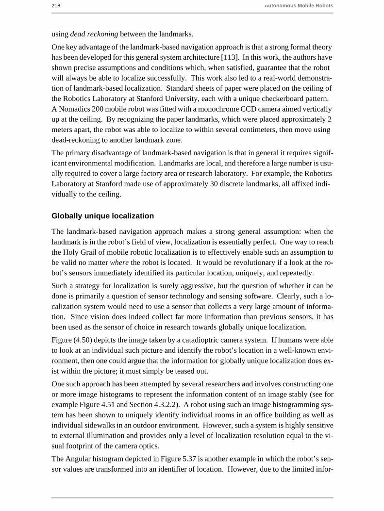
218 Autonomous Mobile Robots
using dead reckoning between the landmarks.
One key advantage of the landmark-based navigation approach is that a strong formal theoryhas been developed for this general system architecture [113]. In this work, the authors haveshown precise assumptions and conditions which, when satisfied, guarantee that the robotwill always be able to localize successfully. This work also led to a real-world demonstra-tion of landmark-based localization. Standard sheets of paper were placed on the ceiling ofthe Robotics Laboratory at Stanford University, each with a unique checkerboard pattern.A Nomadics 200 mobile robot was fitted with a monochrome CCD camera aimed verticallyup at the ceiling. By recognizing the paper landmarks, which were placed approximately 2meters apart, the robot was able to localize to within several centimeters, then move usingdead-reckoning to another landmark zone.
The primary disadvantage of landmark-based navigation is that in general it requires signif-icant environmental modification. Landmarks are local, and therefore a large number is usu-ally required to cover a large factory area or research laboratory. For example, the RoboticsLaboratory at Stanford made use of approximately 30 discrete landmarks, all affixed indi-vidually to the ceiling.
Globally unique localization
The landmark-based navigation approach makes a strong general assumption: when thelandmark is in the robot’s field of view, localization is essentially perfect. One way to reachthe Holy Grail of mobile robotic localization is to effectively enable such an assumption tobe valid no matter where the robot is located. It would be revolutionary if a look at the ro-bot’s sensors immediately identified its particular location, uniquely, and repeatedly.
Such a strategy for localization is surely aggressive, but the question of whether it can bedone is primarily a question of sensor technology and sensing software. Clearly, such a lo-calization system would need to use a sensor that collects a very large amount of informa-tion. Since vision does indeed collect far more information than previous sensors, it hasbeen used as the sensor of choice in research towards globally unique localization.
Figure (4.50) depicts the image taken by a catadioptric camera system. If humans were ableto look at an individual such picture and identify the robot’s location in a well-known envi-ronment, then one could argue that the information for globally unique localization does ex-ist within the picture; it must simply be teased out.
One such approach has been attempted by several researchers and involves constructing oneor more image histograms to represent the information content of an image stably (see forexample Figure 4.51 and Section 4.3.2.2). A robot using such an image histogramming sys-tem has been shown to uniquely identify individual rooms in an office building as well asindividual sidewalks in an outdoor environment. However, such a system is highly sensitiveto external illumination and provides only a level of localization resolution equal to the vi-sual footprint of the camera optics.
The Angular histogram depicted in Figure 5.37 is another example in which the robot’s sen-sor values are transformed into an identifier of location. However, due to the limited infor-
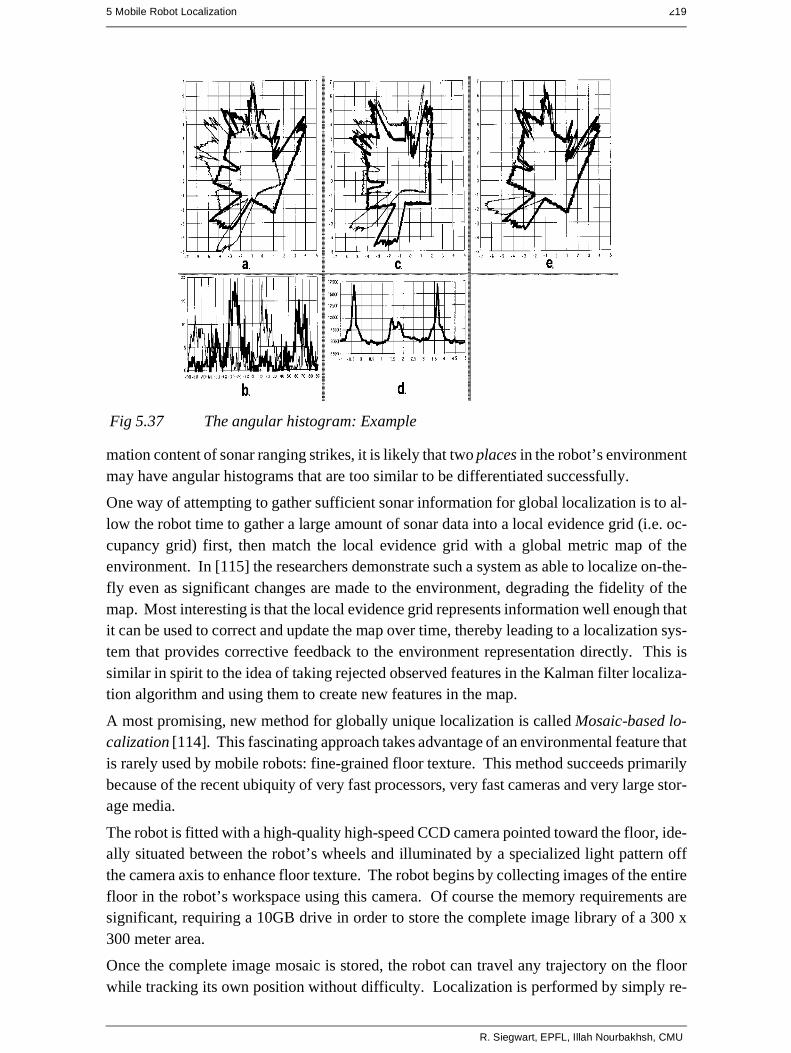
5 Mobile Robot Localization 219
mation content of sonar ranging strikes, it is likely that two places in the robot’s environmentmay have angular histograms that are too similar to be differentiated successfully.
One way of attempting to gather sufficient sonar information for global localization is to al-low the robot time to gather a large amount of sonar data into a local evidence grid (i.e. oc-cupancy grid) first, then match the local evidence grid with a global metric map of theenvironment. In [115] the researchers demonstrate such a system as able to localize on-the-fly even as significant changes are made to the environment, degrading the fidelity of themap. Most interesting is that the local evidence grid represents information well enough thatit can be used to correct and update the map over time, thereby leading to a localization sys-tem that provides corrective feedback to the environment representation directly. This issimilar in spirit to the idea of taking rejected observed features in the Kalman filter localiza-tion algorithm and using them to create new features in the map.
A most promising, new method for globally unique localization is called Mosaic-based lo-calization [114]. This fascinating approach takes advantage of an environmental feature thatis rarely used by mobile robots: fine-grained floor texture. This method succeeds primarilybecause of the recent ubiquity of very fast processors, very fast cameras and very large stor-age media.
The robot is fitted with a high-quality high-speed CCD camera pointed toward the floor, ide-ally situated between the robot’s wheels and illuminated by a specialized light pattern offthe camera axis to enhance floor texture. The robot begins by collecting images of the entirefloor in the robot’s workspace using this camera. Of course the memory requirements aresignificant, requiring a 10GB drive in order to store the complete image library of a 300 x300 meter area.
Once the complete image mosaic is stored, the robot can travel any trajectory on the floorwhile tracking its own position without difficulty. Localization is performed by simply re-
Fig 5.37 The angular histogram: Example
R. Siegwart, EPFL, Illah Nourbakhsh, CMU
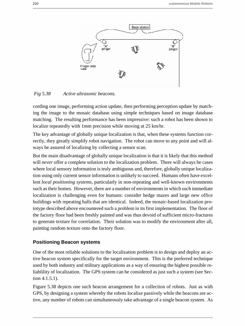
220 Autonomous Mobile Robots
cording one image, performing action update, then performing perception update by match-ing the image to the mosaic database using simple techniques based on image databasematching. The resulting performance has been impressive: such a robot has been shown tolocalize repeatedly with 1mm precision while moving at 25 km/hr.
The key advantage of globally unique localization is that, when these systems function cor-rectly, they greatly simplify robot navigation. The robot can move to any point and will al-ways be assured of localizing by collecting a sensor scan.
But the main disadvantage of globally unique localization is that it is likely that this methodwill never offer a complete solution to the localization problem. There will always be caseswhere local sensory information is truly ambiguous and, therefore, globally unique localiza-tion using only current sensor information is unlikely to succeed. Humans often have excel-lent local positioning systems, particularly in non-repeating and well-known environmentssuch as their homes. However, there are a number of environments in which such immediatelocalization is challenging even for humans: consider hedge mazes and large new officebuildings with repeating halls that are identical. Indeed, the mosaic-based localization pro-totype described above encountered such a problem in its first implementation. The floor ofthe factory floor had been freshly painted and was thus devoid of sufficient micro-fracturesto generate texture for correlation. Their solution was to modify the environment after all,painting random texture onto the factory floor.
Positioning Beacon systems
One of the most reliable solutions to the localization problem is to design and deploy an ac-tive beacon system specifically for the target environment. This is the preferred techniqueused by both industry and military applications as a way of ensuring the highest possible re-liablility of localization. The GPS system can be considered as just such a system (see Sec-tion 4.1.5.1).
Figure 5.38 depicts one such beacon arrangement for a collection of robots. Just as withGPS, by designing a system whereby the robots localize passively while the beacons are ac-tive, any number of robots can simultaneously take advantage of a single beacon system. As
Fig 5.38 Active ultrasonic beacons.
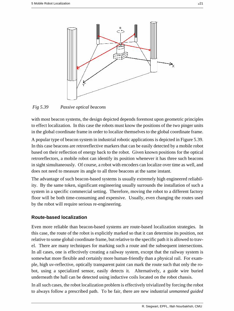
5 Mobile Robot Localization 221
with most beacon systems, the design depicted depends foremost upon geometric principlesto effect localization. In this case the robots must know the positions of the two pinger unitsin the global coordinate frame in order to localize themselves to the global coordinate frame.
A popular type of beacon system in industrial robotic applications is depicted in Figure 5.39.In this case beacons are retroreflective markers that can be easily detected by a mobile robotbased on their reflection of energy back to the robot. Given known positions for the opticalretroreflectors, a mobile robot can identify its position whenever it has three such beaconsin sight simultaneously. Of course, a robot with encoders can localize over time as well, anddoes not need to measure its angle to all three beacons at the same instant.
The advantage of such beacon-based systems is usually extremely high engineered reliabil-ity. By the same token, significant engineering usually surrounds the installation of such asystem in a specific commercial setting. Therefore, moving the robot to a different factoryfloor will be both time-consuming and expensive. Usually, even changing the routes usedby the robot will require serious re-engineering.
Route-based localization
Even more reliable than beacon-based systems are route-based localization strategies. Inthis case, the route of the robot is explicitly marked so that it can determine its position, notrelative to some global coordinate frame, but relative to the specific path it is allowed to trav-el. There are many techniques for marking such a route and the subsequent intersections.In all cases, one is effectively creating a railway system, except that the railway system issomewhat more flexible and certainly more human-friendly than a physical rail. For exam-ple, high uv-reflective, optically transparent paint can mark the route such that only the ro-bot, using a specialized sensor, easily detects it. Alternatively, a guide wire buriedunderneath the hall can be detected using inductive coils located on the robot chassis.
In all such cases, the robot localization problem is effectively trivialized by forcing the robotto always follow a prescribed path. To be fair, there are new industrial unmanned guided
Fig 5.39 Passive optical beacons
R. Siegwart, EPFL, Illah Nourbakhsh, CMU

222 Autonomous Mobile Robots
vehicles that do deviate briefly from their route in order to avoid obstacles. Nevertheless,the cost of this extreme reliability is obvious: the robot is much more inflexible give suchlocalization means, and therefore any change to the robot’s behavior requires significant en-gineering and time.
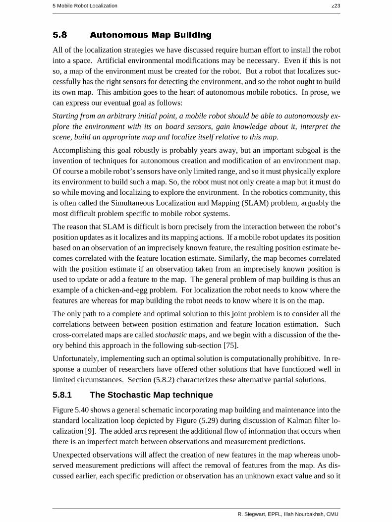
5 Mobile Robot Localization 223
5.8 Autonomous Map Building
All of the localization strategies we have discussed require human effort to install the robotinto a space. Artificial environmental modifications may be necessary. Even if this is notso, a map of the environment must be created for the robot. But a robot that localizes suc-cessfully has the right sensors for detecting the environment, and so the robot ought to buildits own map. This ambition goes to the heart of autonomous mobile robotics. In prose, wecan express our eventual goal as follows:
Starting from an arbitrary initial point, a mobile robot should be able to autonomously ex-plore the environment with its on board sensors, gain knowledge about it, interpret thescene, build an appropriate map and localize itself relative to this map.
Accomplishing this goal robustly is probably years away, but an important subgoal is theinvention of techniques for autonomous creation and modification of an environment map.Of course a mobile robot’s sensors have only limited range, and so it must physically exploreits environment to build such a map. So, the robot must not only create a map but it must doso while moving and localizing to explore the environment. In the robotics community, thisis often called the Simultaneous Localization and Mapping (SLAM) problem, arguably themost difficult problem specific to mobile robot systems.
The reason that SLAM is difficult is born precisely from the interaction between the robot’sposition updates as it localizes and its mapping actions. If a mobile robot updates its positionbased on an observation of an imprecisely known feature, the resulting position estimate be-comes correlated with the feature location estimate. Similarly, the map becomes correlatedwith the position estimate if an observation taken from an imprecisely known position isused to update or add a feature to the map. The general problem of map building is thus anexample of a chicken-and-egg problem. For localization the robot needs to know where thefeatures are whereas for map building the robot needs to know where it is on the map.
The only path to a complete and optimal solution to this joint problem is to consider all thecorrelations between between position estimation and feature location estimation. Suchcross-correlated maps are called stochastic maps, and we begin with a discussion of the the-ory behind this approach in the following sub-section [75].
Unfortunately, implementing such an optimal solution is computationally prohibitive. In re-sponse a number of researchers have offered other solutions that have functioned well inlimited circumstances. Section (5.8.2) characterizes these alternative partial solutions.
5.8.1 The Stochastic Map technique
Figure 5.40 shows a general schematic incorporating map building and maintenance into thestandard localization loop depicted by Figure (5.29) during discussion of Kalman filter lo-calization [9]. The added arcs represent the additional flow of information that occurs whenthere is an imperfect match between observations and measurement predictions.
Unexpected observations will affect the creation of new features in the map whereas unob-served measurement predictions will affect the removal of features from the map. As dis-cussed earlier, each specific prediction or observation has an unknown exact value and so it
R. Siegwart, EPFL, Illah Nourbakhsh, CMU
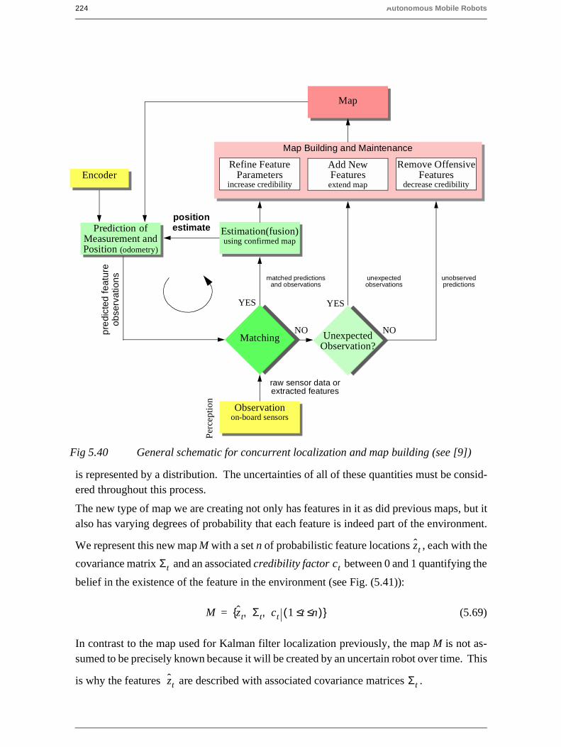
224 Autonomous Mobile Robots
is represented by a distribution. The uncertainties of all of these quantities must be consid-ered throughout this process.
The new type of map we are creating not only has features in it as did previous maps, but italso has varying degrees of probability that each feature is indeed part of the environment.
We represent this new map M with a set n of probabilistic feature locations , each with the
covariance matrix and an associated credibility factor between 0 and 1 quantifying the
belief in the existence of the feature in the environment (see Fig. (5.41)):
(5.69)
In contrast to the map used for Kalman filter localization previously, the map M is not as-sumed to be precisely known because it will be created by an uncertain robot over time. This
is why the features are described with associated covariance matrices .
Observationon-board sensors
Prediction ofMeasurement andPosition (odometry)
Fig 5.40 General schematic for concurrent localization and map building (see [9])
Per
cept
ion
Matching
Estimation(fusion)using confirmed map
raw sensor data orextracted features
pre
dict
edfe
atur
eob
serv
atio
ns
positionestimate
matched predictionsand observations
YES
Encoder
Map
Refine FeatureParameters
increase credibility
Add NewFeatures
extend map
Remove OffensiveFeatures
decrease credibility
Map Building and Maintenance
UnexpectedObservation?
YES
unexpectedobservations
NO NO
unobservedpredictions
zt
Σt ct
M zt Σt ct 1 t n≤ ≤( ), ,{ }=
zt Σt
5 Mobile Robot Localization 225
Just as with Kalman filter localization, the matching step yields has three outcomes in regardto measurement predictions and observations: matched prediction and observations, unex-pected observations and unobserved predictions. Localization, or the position update of therobot, proceeds as before. However, the map is also updated now, using all three outcomesand complete propagation of all the correllated uncertainties (see [9] for more details).
An interesting variable is the credibility factor , which governs the likelihood that the
mapped feature is indeed in the environment. How should the robot’s failure to match ob-served features to a particular map feature reduce that map feature’s credibility? And also,how should the robot’s success at matching a mapped feature increase the chance that themapped feature is "correct?" In [9] the following function is proposed for calculating cred-ibility:
(5.70)
where a and b define the learning and forgetting rate and ns and nu are the number of
matched and unobserved predictions up to time k, respectively. The update of the covari-
ance matrix can be done similarly to the position update seen in previous section. In map-
building the feature positions and the robot’s position are strongly correlated. This forcesus to use a stochastic map, in which all cross-correlations must be updated in each cycle [73,74, 75].
The stochastic map consists of a stacked system state vector:
(5.71)
and a system state covariance matrix:
Cαr
σα2 σαr
σαr σr2
=
x1
y1
x0
y0
Fig 5.41 Uncertainties in the map.
Extracted line
Map feature
Updatedfeature
α
r
rW{ } αW{ }
rS{ } αS{ }
ct
ct k( ) 1 e
ns
a----
nu
b-----–
–
–=
Σt
X xr k( ) x1 k( ) x2 k( ) …xn k( )T
=
R. Siegwart, EPFL, Illah Nourbakhsh, CMU
226 Autonomous Mobile Robots
(5.72)
where the index r stands for the robot and the index i = 1 to n for the features in the map.
In contrast to localization based on an a priori accurate map, in the case of a stochastic mapthe cross-correlations must be maintained and updated as the robot is performing automaticmap-building. During each localization cycle, the cross-correlations robot-to-feature andfeature-to-robot are also updated. In short, this optimal approach requires every value in themap to depend on every other value, and therein lies the reason that such a complete solutionto the automatic mapping problem is beyond the reach of even today’s computational re-sources.
5.8.2 Other Mapping techniques
The mobile robotics research community has spent significant research effort on the prob-lem of automatic mapping, and has demonstrating working systems in many environmentswithout having solved the complete stochastic map problem described earlier. This field ofmobile robotics research is extremely large, and this text will not present a comprehensivesurvey of the field. Instead, we present below two key considerations associated with auto-matic mapping, together with brief discussions of the approaches taken by several automaticmapping solutions to overcome these challenges.
5.8.2.1 Cyclic environments
Possibly the single hardest challenge for automatic mapping to be conquered is to correctlymap cyclic environments. The problem is simple: given an environment that has one ormore loops or cycles (e.g. four hallways that intersect to form a rectangle), create a globallyconsistent map for the whole environment.
This problem is hard because of the fundamental behavior of automatic mapping systems:the maps they create are not perfect. And, given any local imperfection, accumulating suchimperfections over time can lead to arbitrarily large global errors between a map, at the mac-ro level, and the real world, as shown in Figure (5.42). Such global error is usually irrelevantfor mobile robot localization and navigation. After all, a warped map will still serve the ro-bot perfectly well so long as the local error is bounded. However, an extremely large loopstill eventually returns to the same spot, and the robot must be able to note this fact in itsmap. Therefore, global error does indeed matter in the case of cycles.
In some of the earliest work attempting to solve the cyclic environment problem, [116] useda purely topological representation of the environment, reasoning that the topological repre-sentation only captures the most abstract, most important features and avoids a great deal of
Σ
Crr Cr1 Cr2 …Crn
C1r C11 … …C1n
C2r … … …C2n
… … … … …Cnr Cn1 Cn2 …Cnn
=

5 Mobile Robot Localization 227
irrelevant detail. When the robot arrives at a topological node that could be the same as apreviously visited and mapped node (e.g. similar distinguishing features), then the robotpostulates that it has indeed returned to the same node. To check this hypothesis, the robotexplicitly plans and moves to adjacent nodes to see if its perceptual readings are consistentwith the cycle hypothesis.
With the recent popularity of metric maps such as fixed decomposition grid representations,the cycle detection strategy is not as straightforward. Two important features are found inmost autonomous mapping systems that claim to solve the cycle detection problem. First,as with many recent systems, these mobile robots tend to accumulate recent perceptual his-tory to create small-scale local sub-maps [117, 118, 119]. Each sub-map is treated as a sin-gle sensor during the robot’s position update. The advantage of this approach is two-fold.Because odometry is relatively accurate over small distances, the relative registration of fea-tures and raw sensor strikes in a local sub-map will be quite accurate. In addition to this, therobot will have created a virtual sensor system with a significantly larger horizon than itsactual sensor system’s range. In a sense, this strategy at the very least defers the problem ofvery large cyclic environments by increasing the map scale that can be handled well by therobot.
The second recent technique for dealing with cycle environments is in fact a return to thetopological representation. Some recent automatic mapping systems will attempt to identifycycles by associating a topology with the set of metric sub-maps, explicitly identifying the
Fig 5.42 Cyclic Environments: A naive, local mapping strategy with small local er-ror leads to global maps that have a significant error, as demonstrated bythis real-world run on the left. By applying topological correction, the gridmap on the right is extracted [47].
R. Siegwart, EPFL, Illah Nourbakhsh, CMU
228 Autonomous Mobile Robots
loops first at the topological level. In the case of [118] for example, the topological levelloop is identified by a human who pushes a button at a known landmark position. In the caseof [119] the topological level loop is determined by performing correspondence tests be-tween sub-maps, postulating that two sub-maps represent the same place in the environmentwhen the correspondence is good.
One could certainly imagine other augmentations based on known topological methods. Forexample, the globally unique localization methods described in Section (5.7) could be usedto identify topological correctness. It is notable that the automatic mapping research of thepresent has, in many ways, returned to the basic topological correctness question that was atthe heart of some of the earliest automatic mapping research in mobile robotics more than adecade ago. Of course, unlike that early work, today’s automatic mapping results boast cor-rect cycle detection combined with high-fidelity geometric maps of the environment.
5.8.2.2 Dynamic environments
A second challenge extends not just to existing automonous mapping solutions but even tothe basic formulation of the stochastic map approach. All of these strategies tend to assumethat the environment is either unchanging or changes in ways that are virtually insignificant.Such assumptions are certainly valid with respect to some environments, such as for exam-ple the computer science department of a university at 3:00 past midnight. However, in agreat many cases this assumption is incorrect. In the case of wide-open spaces that are pop-ular gathering places for humans, there is rapid change in the freespace and a vast majorityof sensor strikes represent detection of the transient humans rather than fixed surfaces suchas the perimeter wall. Another class of dynamic environments are spaces such as factoryfloors and warehouses, where the objects being stored redefine the topology of the pathwayson a day-to-day basis as shipments are moved in and out.
In all such dynamic environments, an automatic mapping system should capture the salientobjects detected by its sensors and, furthermore, the robot should have the flexibility to mod-ify its map as the position of these salient objects changes. The subject of continuous map-ping, or mapping of dynamic environments is to some degree a direct outgrowth ofsuccessful strategies for automatic mapping of unfamiliar environments. For example, in
the case of stochastic mapping using the credibility factor mechanism, the credibility
equation can continue to provide feedback regarding the probability of existence of variousmapped features after the initial map creation process is ostensibly complete. Thus, a map-ping system can become a map-modifying system by simply continuing to operate. This ismost effective, of course, if the mapping system is real-time and incremental. If map con-struction requires off-line global optimization, then the desire to make small-grained, incre-mental adjustments to the map is more difficult to satisfy.
Earlier we stated that a mapping system should capture only the salient objects detected byits sensors. One common argument for handling the detection of, for instance, humans in
the environment is that mechanisms such as can take care of all features that did not de-
serve to be mapped in the first place. For example, in [117] the authors develop a systembased on a set of local occupany grids (called evidence grids) and a global occupancy grid.
ct
ct

5 Mobile Robot Localization 229
Each time the robot’s most recent local evidence grid is used to update a region of the globaloccupancy grid, extraneous occupied cells in the global occupancy grid are freed if the localoccupancy grid detected no objects (with high confidence) at those same positions.
The general solution to the problem of detecting salient features, however, begs a solutionto the perception problem in general. When a robot’s sensor system can reliably detect thedifference between a wall and a human, using for example a vision system, then the problemof mapping in dynamic environments will become significantly more straightforward.
We have discussed just two important considerations for automatic mapping. There is stilla great deal of research activity focusing on the general map building and localization prob-lem [9, 6, 47, 48, 49, 50, 75, 77]. However, there are few groups working on the generalproblem of probabilistic map building (i.e. stochastic maps) and, so far, a consistent and ab-solutely general solution has yet to be found. This field is certain to produce significant newresults in the next several years, and as the perceptual power of robots improves we expectthe payoff to be greatest here.
R. Siegwart, EPFL, Illah Nourbakhsh, CMU

230 Autonomous Mobile Robots