1

Perception

Maneesh Agrawala

CS 294-10: Visualization Fall 2013

Multidimensional Visualization

2

Position Length Area Volume Value Texture Color Orientation Shape ~8 dimensions?

Visual Encoding Variables

Example: Coffee Sales Sales figures for a fictional coffee chain:

Sales Q-Ratio Profit Q-Ratio Marketing Q-Ratio Product Type N {Coffee, Espresso, Herbal Tea, Tea} Market N {Central, East, South, West}

3

Encode “Sales” (Q) and “Profit” (Q) using Position

Encode “Product Type” (N) using Hue

4

Encode “Market” (N)

using Shape

Encode “Marketing” (Q) using Size

5

Trellis Plots

A trellis plot subdivides space to enable comparison across multiple plots

Typically nominal or ordinal variables are used as dimensions for subdivision

Scatterplot Matrix (SPLOM)

Scatter plots enabling pair-wise comparison of each data dimension

6

Small Multiples [from Wills 95]

select high salaries

avg career HRs vs avg career hits (batting ability)

avg assists vs avg putouts (fielding ability)

how long in majors

distribution of positions played

7

Principal Component Analysis

1. Mean-center the data

2. Find ⊥ basis vectors that maximize the data variance

3. Plot the data using the top vectors

8

Chernoff Faces (1973) Insight: We have evolved a sophisticated ability to interpret facial expression

Idea: Map data variables to facial features Question: Do we process facial features in an uncorrelated way? (i.e., are they separable?)

This is just one example of nD “glyphs”

Parallel Coordinates

9

Parallel Coordinates [Inselberg]

The Multidimensional Detective The Dataset: Production data for 473 batches of a VLSI chip 16 process parameters:

X1: The yield: % of produced chips that are useful X2: The quality of the produced chips (speed)

X3 … X12: 10 types of defects (zero defects shown at top) X13 … X16: 4 physical parameters

The Objective: Raise the yield (X1) and maintain high quality (X2) A. Inselberg, Multidimensional Detective, Proceedings of IEEE Symposium on

Information Visualization (InfoVis '97), 1997

10

Parallel Coordinates

Inselberg’s Principles 1.  Do not let the picture scare you

2.  Understand your objectives –  Use them to obtain visual cues

3.  Carefully scrutinize the picture

4.  Test your assumptions, especially the “I am really sure of’s”

5.  You can’t be unlucky all the time!

11

Each line represents a tuple (e.g., VLSI batch) Filtered below for high values of X1 and X2

Look for batches with nearly zero defects Most of these have low yields à defects OK

12

Notice that X6 behaves differently. Allow 2 defects, including X6 à best batches

Radar Plot / Star Graph

“Parallel” dimensions in polar coordinate space Best if same units apply to each axis

13

Tableau / Polaris

Tableau Research at Stanford: “Polaris” by Stolte, Tang & Hanrahan

14

Tableau

Data Display

Data Model

Encodings

Tableau demo The dataset:   Federal Elections Commission Receipts   Every Congressional Candidate from 1996 to 2002   4 Election Cycles   9216 Candidacies

15

Data Set Schema   Year (Qi)   Candidate Code (N)   Candidate Name (N)   Incumbent / Challenger / Open-Seat (N)   Party Code (N) [1=Dem,2=Rep,3=Other]   Party Name (N)   Total Receipts (Qr)   State (N)   District (N)

  This is a subset of the larger data set available from the FEC, but should be sufficient for the demo

Hypotheses? What might we learn from this data?

16

Hypotheses? What might we learn from this data?

  Has spending increased over time?   Do democrats or republicans spend more money?   Candidates from which state spend the most money?

Tableau Demo

Polaris/Tableau Approach Insight: simultaneously specify both database

queries and visualization

Choose data, then visualization, not vice versa

Use smart defaults for visual encodings

Recently: automate visualization design

(ShowMe – Like APT)

17

Specifying Table Configurations Operands are names of database fields Each operand interpreted as a set {…} Quantitative and Ordinal fields treated differently

Three operators: concatenation (+) cross product (x) nest (/)

Table Algebra: Operands Ordinal fields: interpret domain as a set that partitions

table into rows and columns Quarter = {(Qtr1),(Qtr2),(Qtr3),(Qtr4)} à

Quantitative fields: treat domain as single element set and encode spatially as axes

Profit = {(Profit[-410,650])} à

18

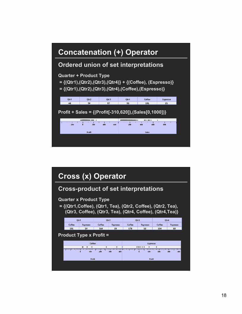
Concatenation (+) Operator Ordered union of set interpretations

Quarter + Product Type = {(Qtr1),(Qtr2),(Qtr3),(Qtr4)} + {(Coffee), (Espresso)} = {(Qtr1),(Qtr2),(Qtr3),(Qtr4),(Coffee),(Espresso)}

Profit + Sales = {(Profit[-310,620]),(Sales[0,1000])}

Cross (x) Operator Cross-product of set interpretations

Quarter x Product Type = {(Qtr1,Coffee), (Qtr1, Tea), (Qtr2, Coffee), (Qtr2, Tea),

(Qtr3, Coffee), (Qtr3, Tea), (Qtr4, Coffee), (Qtr4,Tea)}

Product Type x Profit =

19

Nest (/) Operator Cross-product filtered by existing records

Quarter x Month creates twelve entries for each quarter. i.e., (Qtr1, December)

Quarter / Month creates three entries per quarter based on tuples in database (not semantics)

Polaris/Tableau Table Algebra The operators (+, x, /) and operands (O, Q) provide

an algebra for tabular visualization.

Algebraic statements are then mapped to: Visualizations - trellis plot partitions, visual encodings Queries - selection, projection, group-by aggregation

In Tableau, users make statements via drag-and-drop Note that this specifies operands NOT operators! Operators are inferred by data type (O, Q)

20

Ordinal - Ordinal

Quantitative - Quantitative

21

Ordinal - Quantitative

Querying the Database

22

Summary Visualizing Multiple Dimensions

  Start by visualizing individual dimensions   Avoid “over-encoding”   Use space and small multiples intelligently   Use interaction to generate relevant views

There is rarely a single visualization that answers all questions. Instead, the ability to generate appropriate visualizations quickly is key.

Announcements

23

Assignment 2: Exploratory Data Analysis Use Tableau to formulate & answer questions First steps

  Step 1: Pick a domain   Step 2: Pose questions   Step 3: Find data   Iterate

Create visualizations   Interact with data   Question will evolve   Tableau

Make wiki notebook

  Keep record of all steps you took to answer the questions

Due before class on Sep 30, 2013

Perception

24

Mackinlay’s ranking of encodings QUANTITATIVE ORDINAL NOMINAL

Position Position Position Length Density (Val) Color Hue Angle Color Sat Texture Slope Color Hue Connection Area (Size) Texture Containment Volume Connection Density (Val) Density (Val) Containment Color Sat Color Sat Length Shape Color Hue Angle Length Texture Slope Angle Connection Area (Size) Slope Containment Volume Area Shape Shape Volume

Topics Signal Detection Magnitude Estimation Pre-Attentive Visual Processing Using Multiple Visual Encodings Gestalt Grouping Change Blindness

25

Detection

Detecting brightness

Which is brighter?

26

Detecting brightness

Which is brighter?

(128, 128, 128) (133, 133, 133)

Just noticeable difference JND (Weber’s Law)   Ratios more important than magnitude

  Most continuous variations in stimuli are perceived in discrete steps

27

Information in color and value Value is perceived as ordered

∴ Encode ordinal variables (O)

∴ Encode continuous variables (Q) [not as well]

Hue is normally perceived as unordered

∴ Encode nominal variables (N) using color

Steps in font size Sizes standardized in 16th century

a a a a a a a a a a a a a a a a 6 7 8 9 10 11 12 14 16 18 21 24 36 48 60 72

28

Estimating Magnitude

Compare areas of circles

29

Compare lengths of bars