Perceptual Audio Rendering of Complex Virtual Environments

Nicolas Tsingos, Emmanuel Gallo and George DrettakisREVES/INRIA Sophia-Antipolis∗

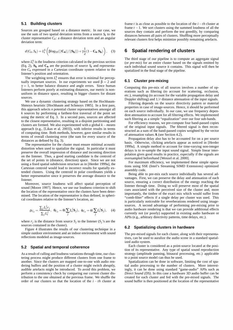
Figure 1: Left, an overview of a test virtual environment, containing 174 sound sources. All vehicles are moving. Mid-left, the magenta dotsindicate the locations of the sound sources while the red sphere represents the listener. Notice that the train and the river are extended sourcesmodeled by collections of point sources. Mid-right, ray-paths from the sources to the listener. Paths in red correspond to the perceptuallymasked sound sources. Right, the blue boxes are clusters of sound sources with the representatives of each cluster in grey. Combination ofauditory culling and spatial clustering allows us to render such complex audio-visual scenes in real-time.

Abstract

We propose a real-time 3D audio rendering pipeline for complexvirtual scenes containing hundreds of moving sound sources. Theapproach, based on auditory culling and spatial level-of-detail, canhandle more than ten times the number of sources commonly avail-able on consumer 3D audio hardware, with minimal decrease inaudio quality. The method performs well for both indoor andoutdoor environments. It leverages the limited capabilities of au-dio hardware for many applications, including interactive architec-tural acoustics simulations and automatic 3D voice management forvideo games.

Our approach dynamically eliminates inaudible sources andgroups the remaining audible sources into a budget number of clus-ters. Each cluster is represented by one impostor sound source, po-sitioned using perceptual criteria. Spatial audio processing is thenperformed only on the impostor sound sources rather than on everyoriginal source thus greatly reducing the computational cost.

A pilot validation study shows that degradation in audio quality,as well as localization impairment, are limited and do not seem tovary significantly with the cluster budget. We conclude that ourreal-time perceptual audio rendering pipeline can generate spatial-ized audio for complex auditory environments without introducingdisturbing changes in the resulting perceived soundfield.

Keywords: Virtual Environments, Spatialized Sound, SpatialHearing Models, Perceptual Rendering, Audio Hardware.

∗contact Nicolas.Tsingos@sophia.inria.fr or visithttp://www-sop.inria.fr/reves/

1 Introduction

Including spatialized audio is a key aspect in producing realistic vir-tual environments. Recent studies have shown that the combinationof auditory and visual cues enhances the sense of immersion (e.g.,[Larsson et al. 2002]). Unfortunately, high-quality spatialized au-dio rendering based on pre-recorded audio samples requires heavysignal processing, even for a small number of sound sources. Suchprocessing typically includes rendering of source directivity pat-terns [Savioja et al. 1999], 3D positional audio [Begault 1994] andartificial reverberation [Gardner 1997; Savioja et al. 1999].

Despite advances in commodity audio hardware (e.g., [Sound-Blaster 2004]), only a small number of processing channels (16 to64) are usually available, corresponding to the number of sourcesthat can be simultaneously rendered.

Although point-sources can be used to simulate direct and low-order indirect contributions interactively using geometric tech-niques [Funkhouser et al. 1999], a large number of secondary“images-sources” are required if further indirect contributions are tobe added [Borish 1984]. In addition, many real-world sources suchas a train (see Figure 1) are extended sound sources; one solutionallowing their improved, if not correct, representation is to simulatethem with a collection of point sources, as proposed in [Sensaura2001]. This further increases the number of sources to render. Thisalso applies to more specific effects, such as rendering of aerody-namic sounds [Dobashi et al. 2003], that also require processingcollections of point sources.

For all the reasons presented above, current state-of-the-art solu-tions [Tsingos et al. 2001; Fouad et al. 2000; Wenzel et al. 2000;Savioja et al. 1999], still cannot provide high-quality audio render-ings for complex virtual environments which respect the manda-tory real-time constraints, since the number of sources required isnot supported by hardware, and software processing would be over-whelming.

To address this shortcoming, we propose novel algorithms per-mitting high-quality spatial audio rendering for complex virtual en-vironments, such as that shown in Figure 1. Our work is based onthe observation that audio rendering operations (see Figure 2) areusually performed for every sound source while there is significantpsycho-acoustic evidence that this might not be necessary due tolimits in our auditory perception and localization accuracy [Moore1997; Blauert 1983].

Similar to the occlusion culling and level of detail algorithmswidely used in computer graphics [Funkhouser and Sequin 1993],we introduce a dynamic sorting and culling algorithm and a spatialclustering technique for 3D sound sources that allows for 1) sig-nificantly reducing the number of sources to render, 2) amortizingcostly spatial audio processing over groups of sources and 3) lever-aging current commodity audio hardware for complex auditory sim-ulations. Contrary to prior work in audio rendering, we exploit apriori knowledge of the spectral characteristics of the input soundsignals to optimize rendering. From this information, we interac-tively estimate the perceptual saliency of each sound source presentin the environment. This saliency metric drives both our culling andclustering algorithms.

We have implemented a system combining these approaches.The results of our tests show that our solution can render highlydynamic audio-visual virtual environments comprising hundreds ofpoint-sound sources. It adapts well to a variety of applications in-cluding simulation of extended sound sources and indoor acousticssimulation using image-sources to model sound reflections.

We also present the results of a pilot user study providing a firstvalidation of our choices. In particular, it shows that our algorithmshave little impact on the perceived audio quality and spatial audiolocalization cues when compared to reference renderings.

Audio scenedescription

Positions of sources and listener

Reverberation

resamplingsource directivityequalizationocclusion filtering

Mix Sound output

+

Waveform audio data

Traditional pipeline

Audio hardware (APU)

pre-mixing positional audio

Figure 2: A traditional hardware-accelerated audio renderingpipeline. Pre-mixing can usually be implemented with few oper-ations while positional audio and reverberation rendering requireheavier processing.

2 Related Work

Our approach builds upon prior work in the fields of perceptualaudio coding and audio rendering. The following sections give ashort overview of the background most relevant to our problem.

Perceptual audio coding and sound masking

When a large number of sources are present in the environment, itis very unlikely that all will be audible due to masking occurring inthe human auditory system [Moore 1997].

This masking mechanism has been successfully exploited in per-ceptual audio coding (PAC), such as the well known MPEG I Layer3 (mp3) standard [Painter and Spanias 1997; Brandenburg 1999].Note that contrary to PAC, our primary goal is to detect maskingoccurring between several sounds in a dense sound mixture ratherthan “intra-sound” masking. Since our scenes are highly dynamic,masking thresholds have to be continuously updated. This requiresan efficient evaluation of the necessary information.

Interactive masking evaluation has also already been used forefficient modal synthesis [Lagrange and Marchand 2001; van denDoel et al. 2002; van den Doel et al. 2004] but, to our knowledge, nosolution to date has been proposed to dynamically evaluate maskingfor mixtures of general digitally recorded sounds. Such techniquescould nevertheless complement our approach for real-time synthe-sized sounds effects.

In the context of spatialized audio, binaural masking (i.e., takinginto account the signals reaching both ears) is of primary impor-tance. Although mp3 allows for joint-stereo coding, very few PACapproaches aim at encoding spatial audio and include the necessarybinaural masking evaluation. This is quite a complex task sincebinaural masking thresholds are not entirely based on the spatial lo-cation of the sources but also depend on the relative phase of thesignals at each ear [Moore 1997]. Finally, in the context of roomacoustics simulation, several perceptual studies aimed at evaluatingmasking thresholds of individual reflections were conducted usingsimple image-sources simulations [Begault et al. 2001]. Unfortu-nately, no general purpose thresholds were derived from this work.

Spatial audio rendering

Few solutions to date have been proposed which reduce the over-all cost of an audio rendering pipeline. Most of them specifi-cally target the filtering operations involved in spatial audio ren-dering. Martens and Chen et al. [1987; 1995] proposed the useof principal component analysis of Head Related Transfer Func-tions (HRTFs) to speed up the signal processing operations. Oneapproach, however, optimizes HRTF filtering by avoiding the pro-cessing of psycho-acoustically insignificant spectral components ofthe input signal [Filipanits 1994].

Fouad et al. [1997] propose a level-of-detail rendering approachfor spatialized audio where the sound samples are progressivelygenerated based on a perceptual metric in order to respect a bud-get computing time. When the budget processing time is reached,missing samples are interpolated from the calculated ones. Sincefull processing still has to be performed on a per source basis, theapproach might result in significant degradation for large numbersof sources. Despite these advances, high-quality rendering of com-plex auditory scenes still requires dedicated multi-processor sys-tems or distributed audio servers [Chen et al. 2002; Fouad et al.2000].

An alternative to software rendering is to use additional re-sources such as high-end DSP systems (Tucker Davis, Lake DSP,etc.) or commodity audio hardware (e.g., Sound Blaster [Sound-Blaster 2004]). The former are usually high audio fidelity systemsbut are not widely available and usually support ad-hoc APIs. Thelatter provide hardware support for game-oriented APIs (e.g., Di-rect Sound 3D [Direct Sound 3D 2004], and its extensions such asEAX [EAX 2004]). Contrary to high-end systems, they are widelyavailable, inexpensive and tend to become de facto standards. Bothclasses of systems provide specialized 3D audio processing for avariety of listening setups and additional effects such as reverber-ation processing. In both cases, however, only a small number ofsources (typically 16 to 64) can be rendered using hardware chan-nels. Automatic adaptation to resources is available in Direct Soundbut is based on distance-culling (far-away sources are simply notrendered) which can lead to discontinuities in the generated audiosignal. Moreover, this solution would fail when many sources areclose to the listener.

A solution to the problem of rendering many sources usinglimited software or hardware resources has been presented byHerder [1999a; 1999b] and is based on a clustering strategy. Sim-ilar approaches have also been proposed in computer graphics foroff-line rendering of scenes with many lights [Paquette et al. 1998].In Herder [1999a; 1999b], a potentially large number of point-sound sources can be down-sampled to a limited number of rep-resentatives which are then used as actual sources for rendering. Intheory, such a framework is general and can accommodate primarysound sources and image-sources. Herder’s clustering scheme isbased on fixed clusters, corresponding to a non-uniform spatial sub-division, which cannot be easily adapted to fit a pre-defined budget.Hence, the algorithm cannot be used as is for resource manage-ment purposes. Second, the choice of the cluster representative (the

Audio scenedescription

Positions of sources and listener

Sound outputcluster pre-mixing

resamplingsource directivityequalizationocclusion filtering

CPU APU

positional audio

Reverberation

Mix

+

PerceptualCulling

ClusteringWaveformaudio data

Perceptual rendering pipeline

InstantaneousPower spectrum &

Tonality index

cluster representative

Perceptual importance

Figure 3: Our novel approach combining a perceptual culling/clustering strategy to reduce the number of sources and amortize costly opera-tions over groups of sound sources.

Cartesian centroid of all sources in the cluster) is not optimal in thepsycho-acoustical sense since it does not account for the character-istics of the input audio signals.

3 Overview of our contributions

We propose a novel spatial audio rendering pipeline for sampledsound signals. Our approach can be decomposed into four steps(see Figure 3) repeated for each audio processing frame throughtime (typically every 20 to 30 milliseconds):

• First, we evaluate the perceptual saliency of all sources in thescene. After sorting all sources based on their binaural loud-ness, we cull perceptually inaudible sources by progressivelyinserting sources into the mix until their combination masksall remaining ones. This stage requires the pre-computationof some spectral information for each input sound signal.

• We then group the remaining sound sources into a predefinedbudget number of clusters. We use a dynamic clustering algo-rithm based on the Hochbaum-Shmoys heuristic [Hochbaumand Schmoys 1985], taking into account the loudness of eachsource. A representative point source is constructed for eachnon-empty cluster.

• Then, an equivalent source signal is generated for each clusterin order to feed the available audio hardware channels. Thisphase involves a number of operations on the original audiodata (filtering, re-sampling, mixing, etc.) which are differentfor each source.

• Finally, the pre-mixed signals for each cluster together withtheir representative point location can be used to feed audiorendering hardware through standard APIs (e.g., Direct Sound3D), or can be rendered in software.

Sections 4 to 7 detail each of these steps. We have also conducted apilot perceptual study with 20 listeners showing that our approachhas very limited impact on audio quality and localization abilities.The results of this study are discussed in Section 8.

4 Perceptual saliency of sound sources

The first step of our algorithm aims at evaluating the perceptualsaliency of every source. Saliency should reflect the perceptual im-portance of each source relative to the global soundscape.

Perception of multiple simultaneous sources is a complex prob-lem which is actively studied in the community of auditory sceneanalysis (ASA) [Bregman 1990; Ellis 1992] where perceptual orga-nization of the auditory world follows the principles of Gestalt psy-chology. However, computational ASA usually attempts to solvethe inverse and more complex problem of segregating a complexsound mixture into discrete, perceptually relevant auditory events.This requires heavy processing in order to segment pitch, timbreand loudness patterns out of the original mixture and remains ap-plicable only to very limited cases.

In our case, we chose the binaural loudness as a possible saliencymetric. Due to sound masking occurring in our hearing process,some of the sounds in the environment might not be audible. Oursaliency estimation accounts for this phenomenon by dynamicallyevaluating masked sound sources.

4.1 Pre-processing the audio data

In this paper, we focus on applications where the input audio sam-ples are known in advance (i.e., do not come from a real-time inputand are not synthesized in real-time). Based on this assumption, wecan pre-compute spectral features of our input signals throughouttheir duration and dynamically access them at runtime.

Specifically, for each input signal, we generate instantaneousshort-time power spectrum distribution (PSD) and tonality indexfor a number of frequency sub-bands. Such features are widelyused in perceptual audio coding [Painter and Spanias 1997].

The PSD measures the energy present in each frequency band,while the tonality index is an indication of the signal noisiness: lowindices indicate a noisier component. This index will be used forinteractive estimation of masking thresholds.

Our input sound signals were sampled at 44100 Hz. In order toretain efficiency, we use four frequency bands f corresponding to0-500 Hz, 500-2000 Hz, 2000-8000 Hz and 8000-22050 Hz. Al-though this is far less than the 25 critical bands used in audio cod-ing, we found it worked well in practice for our application whilelimiting computational overhead.

We derive our spectral cues from a short time fast Fourier trans-form (FFT) [Steiglitz 1996]. We used 1024 sample long Hanning-windowed frames with 50% overlap. We store for each band f itsinstantaneous power spectrum distribution (i.e., the integral of thesquare of the modulus of the Fourier transform), PSDt( f ), for eachframe t.

From the PSD, we estimate a log-scale spectral flatness measureof the signal as:

SFMt( f ) = 10 log10

(µg(PSDt( f ))µa(PSDt( f ))

),

where µg and µa are respectively the geometric and arithmetic meanof the PSD over all FFT bins contained in band f . We then estimatethe tonality index, Tt( f ), as:

Tt ( f ) = min(SFMt ( f )

−60,1).

Note that, as a result, Tt( f ) ∈ [0,1].This information is quite compact (8 floating-point values per

frame, i.e., 1.4 kbyte per second of input audio data at CD quality)and does not result in significant memory overhead.

This pre-processing can be done off-line or when the applicationis started but can also be performed in real-time for a small numberof input signals since our unoptimized implementation runs aboutsix times faster than real-time.

4.2 Binaural loudness estimation

At any given time-frame t of our audio rendering simulation, eachsource Sk is characterized by : 1) its distance to the listener r, 2) thecorresponding propagation delay δ = r/c, where c is the speed ofsound, and 3) a frequency-dependent attenuation A which consistsin a scalar factor for each frequency band. A is derived from theoctave band attenuation values of the various filters used to alter thesource signal, such as occlusion, scattering and directivity filters.For additional information on these filters see [Pierce 1984; ANSI1978; Tsingos and Gascuel 1997; Savioja et al. 1999]. For instance,in the case of a direct, unoccluded contribution from the source tothe receiver, A will simply be the attenuation in each frequencyband due to atmospheric scattering effects. If the sound is furtherreflected or occluded, A will be obtained as the product of all scalarattenuation factors along the propagation path.

Our saliency estimation first computes the perceptual loudnessat time t, of each sound source k, using an estimate of the soundpressure level in each frequency band. This estimate pressure levelis computed at each ear as:

Pkt ( f ) = Spat(Sk)×

√PSDk

t−δ( f )×Akt ( f )/r, (1)

where Spat(Sk) returns a direction and frequency dependent atten-uation due to the spatial rendering (e.g., HRTF processing). In ourcase, we estimated this function using measurements of the outputlevel of band-passed noise stimuli rendered with Direct Sound 3Don our audio board.

As a result, Equation 1 must be evaluated twice since theSpat(Sk) values will be different for the left and right ear.

The loudness values at both ears Lleftkt and Lrightkt , are then

obtained from the sound pressure levels at each ear using the modelof [Moore et al. 1997]. Loudness, expressed in phons, is a measureof the subjective intensity of a sound referenced to a 1kHz tone1.Based on Moore’s model, we pre-compute a loudness table for eachof our four frequency sub-bands assuming the original signal is awhite noise. We use these tables to directly obtain a loudness valueper frequency band given the value of Pk

t ( f ) at both ears.Going back to linear scale, a scalar binaural loudness criterion

Lkt is computed as:

Lkt = ||10Lleftk

t /20||2 + ||10Lrightkt /20||2. (2)

Finally, we normalize this estimate and average it over a numberof audio frames to obtain smoothly varying values (we typicallyaverage over 0.1-0.3 sec. i.e., 4-12 frames).

1by definition phons are equal to the sound pressure level, expressed indecibels, of a 1kHz sine wave.

4.3 Binaural masking and perceptual culling

We evaluate masking in a conservative manner by first sorting thesources by decreasing order according to their normalized loudnessLk

t and progressively inserting them into the current mix until theymask the remaining ones.

We start by computing the total power level of our scene

PTOT = ∑k

Pkt ( f ).

At each frame, we maintain the sum of the power of all sourcesto be added to the mix, PtoGo, which is initially equal to PTOT.

We then progressively add sources to the mix, maintaining thecurrent tonality Tmix, masking threshold Mmix, as well as the cur-rent power Pmix of the mix. We assume that sound power addsup which is a crude approximation but works reasonably well withreal-world signals, which are typically noisy and uncorrelated.

To perform the perceptual culling, we apply the following algo-rithm, where ATH is the absolute threshold of hearing (correspond-ing to 2 phons) [Moore 1997]:

Mmix = −200Pmix = 0T = 0PtoGo = PTOT

while (dB(PtoGo) > dB(Pmix) − Mmix) and (PtoGo > ATH) doadd source Sk to the mixPtoGo − = Pk

Pmix + = Pk

T + = Pk ∗Tk

Tmix = T/Pmix

Mmix = (14.5+Bark(fmax))∗Tmix +5.5∗ (1−Tmix)k++

end

Similar to prior audio coding work [Painter and Spanias 1997],we estimate the masking threshold, Mmix( f ) as:

Mmix( f ) = (14.5+Bark(fmax))∗Tmix( f )+ 5.5∗ (1−Tmix( f )) (dB),

where Bark(fmax) is the value of the maximum frequency in eachfrequency-band f expressed in Bark scale. The Bark scale is a map-ping of the frequencies in Hertz to Bark numbers, corresponding tothe 25 critical bands of hearing [Zwicker and Fastl 1999]. In ourcase we have for our four bands: Bark(500) = 5,Bark(2000) =18,Bark(8000) = 24,Bark(22050) = 25.

The masking threshold represents the limit below which a mas-kee is going to be masked by the considered signal.

To better account for binaural masking phenomena, we evaluatemasking for left and right ears and assume the culling process isover when the remaining power at both ears is below the maskingthreshold of the current mix.

Since we always maintain an overall estimate for the power ofthe entire scene, our culling algorithm behaves well even in the caseof a scene composed of many low-power sources. This is the casefor instance with image-sources resulting from sound reflections. Anaive algorithm might have culled all sources while their combina-tion is actually audible.

5 Dynamic clustering of sound sources

Sources that have not been culled by the previous stage are thengrouped by our dynamic clustering algorithm. Each cluster will actas a new point source representing all the sources it contains (i.e.,a point source with a complex impulse response). Our goal is toensure minimal perceptible error between these auditory impostorsand the original auditory scene.

5.1 Building clusters

Sources are grouped based on a distance metric. In our case, weuse the sum of two spatial deviation terms from a source Sk to thecluster representative Cn: a distance deviation term and an angulardeviation term:

d(Cn,Sk) = Lkt

(βlog10(||Cn||/||Sk||)+ γ

12(1−Cn.Sk)

), (3)

where Lkt is the loudness criterion calculated in the previous section

(Eq. 2), Sk and Cn are the positions of source Sk and representa-tive Cn expressed in a Cartesian coordinate system relative to thelistener’s position and orientation.

The weighting term Lkt ensures that error is minimal for percep-

tually important sources. In our experiments we used β = 2 andγ = 1, to better balance distance and angle errors. Since humanlisteners perform poorly at estimating distances, our metric is non-uniform in distance space, resulting in bigger clusters for distantsources.

We use a dynamic clustering strategy based on the Hochbaum-Shmoys heuristic [Hochbaum and Schmoys 1985]. In a first pass,this approach selects n potential cluster representatives amongst allk sources by performing a farthest-first traversal of the point setusing the metric of Eq. 3. In a second pass, sources are affectedto the closest representative, resulting in a disjoint partitioning andclusters are formed. We also experimented with a global k−meansapproach (e.g., [Likas et al. 2003]), with inferior results in termsof computing time. Both methods, however, gave similar results interms of overall clustering error (the sum for every source of thedistances as defined by Eq. 3).

The representative for the cluster must ensure minimal acousticdistortion when used to spatialize the signal. In particular it mustpreserve the overall impression of distance and incoming directionon the listener. Thus, a good starting candidate is the centroid ofthe set of points in (distance, direction) space. Since we are notusing a fixed spatial subdivision structure as in [Herder 1999a], theCartesian centroid would lead to incorrect results for spatially ex-tended clusters. Using the centroid in polar coordinates yields abetter representative since it preserves the average distance to thelistener.

Moreover, source loudness will affect spatial perception ofsound [Moore 1997]. Hence, we use our loudness criterion to shiftthe location of the representative once the clusters have been deter-mined. The location of the representative is thus defined, in spheri-cal coordinates relative to the listener’s location, as:

ρCn =∑ j L j

t r j

∑ j L jt

, θCn = θ(∑j

L jt S j), φCn = φ(∑

jL j

t S j), (4)

where r j is the distance from source Sj to the listener (S j’s are thesources contained in the cluster).

Figure 4 illustrates the results of our clustering technique in asimple outdoor environment and an indoor environment with soundreflections modeled as image-sources.

5.2 Spatial and temporal coherence

As a result of culling and loudness variations through time, our clus-tering process might produce different clusters from one frame toanother. Since the clusters are mapped one-to-one with audio ren-dering buffers and the position of a cluster might switch abruptly,audible artefacts might be introduced. To avoid this problem, weperform a consistency check by comparing our current cluster dis-tribution to the one obtained at the previous frame. We shuffle theorder of our clusters so that the location of the i− th cluster at

frame t is as close as possible to the location of the i− th cluster atframe t −1. We sort clusters using the summed loudness of all thesources they contain and perform the test greedily, by comparingdistances between all pairs of clusters. Shuffling more perceptuallyrelevant clusters first helps minimize possibly remaining artefacts.

6 Spatial rendering of clusters

The third stage of our pipeline is to compute an aggregate signal(or pre-mix) for an entire cluster based on the signals emitted byeach individual sound source it contains. This signal will then bespatialized in the final stage of the pipeline.

6.1 Cluster pre-mixing

Computing this pre-mix of all sources involves a number of op-erations such as filtering (to account for scattering, occlusion,etc.), resampling (to account for the variable propagation delay andDoppler shifting) and 1/r distance attenuation of the input signals.

Filtering depends on the source directivity pattern or materialproperties in case of image-sources. Hence, it should be performedon each source individually. In our case, we use frequency depen-dent attenuation to account for all filtering effects. We implementedsuch filtering as a simple “equalization” over our four sub-bands.

For efficiency reasons, we pre-compute four band-passed copiesof the original input signals. The filtered signal is then recon-structed as a sum of the band-passed copies weighted by the vectorof attenuation values A (see Section 4.2).

Propagation delay also has to be accounted for on a per sourcebasis. Otherwise, clicking artefacts appear as noticed in [Herder1999a]. A simple method to account for time-varying non-integerdelays is to re-sample the input sound signal. Simple linear inter-polation gives good results in practice, especially if the signals areoversampled beforehand [Wenzel et al. 2000].

For maximum efficiency, we implemented these simple opera-tions using SSE (Intel’s Streaming SIMD Extensions) optimizedassembly code.

Being able to pre-mix each source individually has several ad-vantages. First, we can preserve the delay and attenuation of eachsource, ensuring a correct distribution of the energy reaching thelistener through time. Doing so will preserve most of the spatialcues associated with the perceived size of the cluster and, moreimportantly, the timbre of the exact mix which would suffer from“comb-filter” effects if a single delay per cluster was used. Thisis particularly noticeable for reverberations rendered using image-sources. A second advantage of performing pre-mixing prior toaudio hardware rendering is that we can provide additional effectscurrently not (or poorly) supported in existing audio hardware orAPIs (e.g., arbitrary directivity patterns, time delays, etc.).

6.2 Spatializing clusters in hardware

The pre-mixed signals for each cluster, along with their representa-tives, can be used to auralize the audio scene in a standard spatial-ized audio system.

Each cluster is considered as a point-source located at the posi-tion of its representative. Any type of spatial sound reproductionstrategy (amplitude panning, binaural processing, etc.) applicableto a point source model can thus be used.

Spatialization can be done in software, limiting the cost of spa-tial audio processing to the number of clusters. More interest-ingly, it can be done using standard “game-audio” APIs such asDirect Sound (DS). In this case a hardware 3D audio buffer can becreated for each cluster and fed with the pre-mixed signals. Thesound buffer is then positioned at the location of the representative

Figure 4: Top row: note how the four clusters (in blue) adapt to the listener’s location (shown in red). Bottom row: a clustering example withimage-sources in a simple building environment (seen in top view). The audible image-sources, shown in green in the right-hand side image,correspond to the set of reflection paths (shown in white) in the left-hand side image.

(e.g., using DS SetPosition command). We synchronize all posi-tional commands at the beginning of each audio frame using DSnotification mechanism. We also use a simple cross-fading schemeby computing a few extra samples at each frame and blending themwith the first samples of the next prior to the spatialization. Thiseliminates artefacts resulting from sources moving in or out of clus-ters. In our current implementation, we use a 100-sample overlapat 44.1kHz (i.e., 2ms or about a tenth of our audio frame).

Since audio hardware usually performs sampling-rate conver-sion, it is also possible to assign a different rate to each clusterdepending on its importance. We define the importance of a clusteras the sum of the loudness values of all the sources it contains. Wesort the clusters by decreasing importance prior to rendering, andmap them to a set of hardware buffers whose sampling rate is de-creasing, hence requiring less data to be rendered for an equivalenttime-step. This is similar in spirit to the approach of [Fouad et al.1997] but does not require extra software processing and better in-tegrates with current hardware rendering pipelines.

Finally, we can also benefit from additional processing offeredby current consumer audio hardware, such as artificial reverberationprocessing, as demonstrated in the video (see the trainstation androom acoustics sequences).

7 Applications and performance tests

We evaluated our algorithms on two prototype applications: 1) ren-dering of one exterior (Highway) and one interior (Trainstation)scene with numerous point sound sources and 2) rendering of aninterior scene (Busy office) including modeling of sound reflections.

All tests were conducted on a Pentium 4 3GHz PC with a nVidiaGeForce FX5800 ultra graphics accelerator and a CreativeLabs Au-digy2 platinum Ex audio board. Audio was rendered using 1200-sample long audio frames at 44.1kHz.

Our first two examples feature extended sound sources resultingin many point sources to render. In our case, extended sources arecollections of several point sources playing potentially different sig-nals (e.g., the helicopter has 4 sound sources for rotors, jet exhaustand engine, the river is modeled with 40 point sources, etc.). Eachsound source can have its own location, orientation and directiv-ity function (e.g., the directivity of the jet exhaust of the helicopterand voice of the pedestrians in the train station are modeled usingfrequency dependent cosine lobes).

The train station example contains 60 people, with a soundsource for their footsteps and one for their voices, two trains, with asource at each wheel, and a number of other sources (pigeons, etc.).A total of 195 sound sources are included. The highway scene con-tains 100 vehicles and environmental sound effects resulting in 174

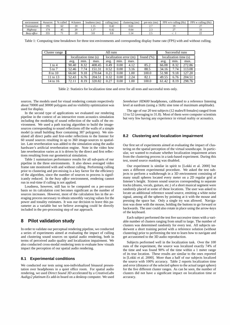
environment #sources % culled #clusters loudness (ms) culling (ms) clustering (ms) pre-mix (ms) FPS w/o culling (Hz) FPS w culling (Hz)Trainstation 195 62 20 1.15 0.42 0.61 2.7 19 27

Highway 174 45 20 1.17 0.42 0.64 2.3 27 33Busy office 355 71 20 3.8 0.8 1.14 2.5 < 1 22

Table 1: Computing time breakdown for three test environments and corresponding display frame rate (FPS) with and without culling.

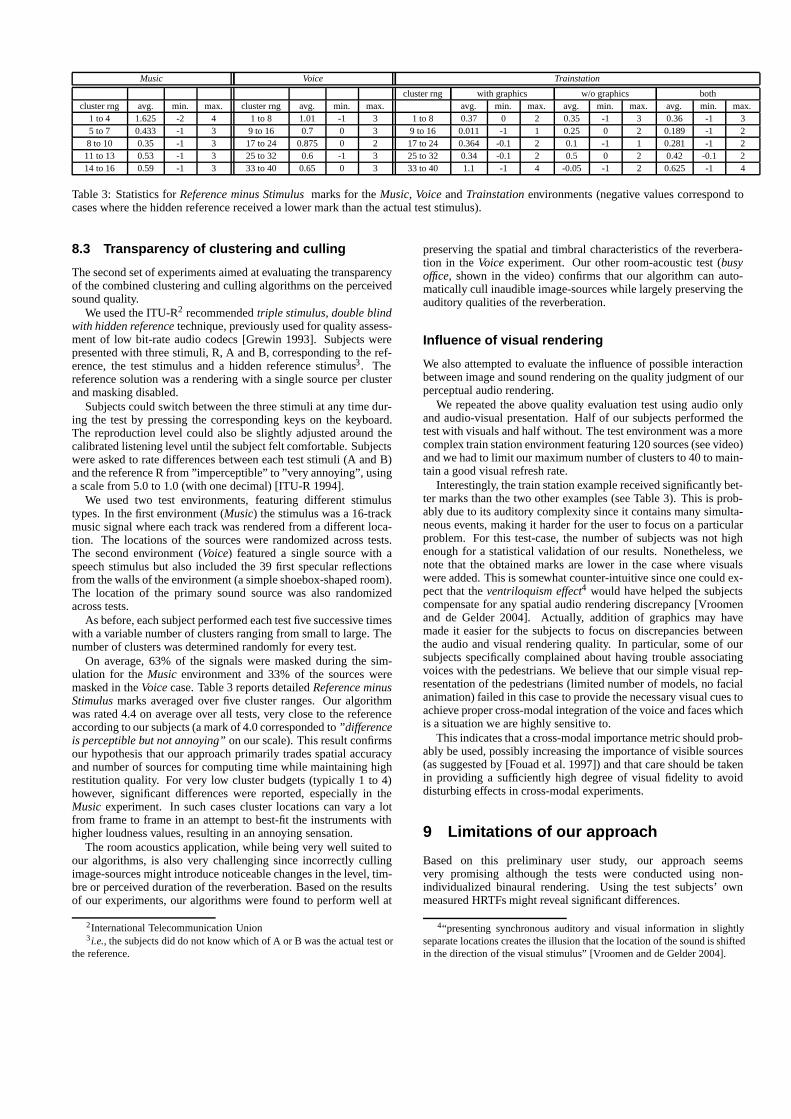
Cluster range All runs Successful runslocalization time (s) localization error (m) found (%) localization time (s)

avg. min. max. avg. min. max. avg. min. max.1 to 4 90.40 8.32 408.45 0.49 0.00 4.12 85.2 66.08 8.32 272.865 to 7 52.46 7.74 151.31 0.52 0.00 3.16 88.5 34.16 7.74 113.088 to 10 66.60 9.18 270.64 0.21 0.00 1.00 100.0 51.98 9.18 127.20

11 to 13 52.43 6.76 204.51 0.32 0.00 2.24 82.1 49.55 6.76 204.5114 to 16 72.11 8.19 320.82 0.27 0.00 1.00 100.0 61.42 8.19 298.76

Table 2: Statistics for localization time and error for all tests and successful tests only.

sources. The models used for visual rendering contain respectivelyabout 70000 and 30000 polygons and no visibility optimization wasused for display.

In the second type of applications we evaluated our renderingpipeline in the context of an interactive room acoustics simulationincluding the modeling of sound reflection of the walls of the en-vironment. We used a path tracing algorithm to build the image-sources corresponding to sound reflections off the walls of a simplemodel (a small building floor containing 387 polygons). We sim-ulated all direct paths and first-order reflections to the listener for60 sound sources resulting in up to 360 image-sources to spatial-ize. Late reverberation was added to the simulation using the audiohardware’s artificial reverberation engine. Note in the video howlate reverberation varies as it is driven by the direct and first reflec-tions resulting from our geometrical simulation.

Table 1 summarizes performance results for all sub-parts of ourpipeline in the three environments. It also shows averaged videoframe rate monitored with and without culling. Performing cullingprior to clustering and pre-mixing is a key factor for the efficiencyof the algorithm, since the number of sources to process is signif-icantly reduced. In the busy office environment, rendering cannotrun in real-time if culling is not applied.

Loudness, however, still has to be computed on a per-sourcebasis so its calculation cost becomes significant as the number ofsources increases. However, most of the calculation lies in the av-eraging process necessary to obtain smoothly varying values for thepower and tonality estimates. It was our decision to leave this pa-rameter as a variable but we believe averaging could be directlyincluded in the pre-processing step of our approach.

8 Pilot validation study

In order to validate our perceptual rendering pipeline, we conducteda series of experiments aimed at evaluating the impact of cullingand clustering sound sources on spatial audio rendering, both interms of perceived audio quality and localization impairment. Wealso conducted cross-modal rendering tests to evaluate how visualsimpact the perception of our spatial audio rendering.

8.1 Experimental conditions

We conducted our tests using non-individualized binaural presen-tation over headphones in a quiet office room. For spatial audiorendering, we used Direct Sound 3D accelerated by a CreativeLabsAudigy2 platinum Ex add-in board on a desktop computer. We used

Sennheiser HD600 headphones, calibrated to a reference listeninglevel at eardrum (using a 1kHz sine tone of maximum amplitude).

The age of our 20 test subjects (12 males/8 females) ranged from13 to 52 (averaging to 31.8). Most of them were computer scientistsbut very few having any experience in virtual reality or acoustics.

8.2 Clustering and localization impairment

Our first set of experiments aimed at evaluating the impact of clus-tering on the spatial perception of the virtual soundscape. In partic-ular, we wanted to evaluate whether localization impairment arisesfrom the clustering process in a task-based experiment. During thistest, sound source masking was disabled.

Our experiment is similar in spirit to [Lokki et al. 2000] butuses a different experimental procedure. We asked the test sub-jects to perform a walkthrough in a 3D environment consisting ofmany small spheres located every meter on a 2D regular grid atlistener’s height. Sixteen sound sources corresponding to separatetracks (drums, vocals, guitars, etc.) of a short musical segment wererandomly placed at some of these locations. The user was asked tolocate an additional reference sound source, emitting a white noisesignal, among all the spheres by pointing at it with the mouse andpressing the space bar. Only a single try was allowed. Naviga-tion was done with the mouse, holding the buttons to go forward orbackwards. The user could also rotate in place using the arrow-keysof the keyboard.

Each subject performed the test five successive times with a vari-able number of clusters ranging from small to large. The number ofclusters was determined randomly for every test. All subjects un-derwent a short training period with a reference solution (withoutclustering) prior to performing the test to learn how to navigate andget accustomed to the 3D audio reproduction.

Subjects performed well in the localization task. Over the 100runs of the experiment, the source was localized exactly 74% ofthe time and was found 90% of the time within a 1 meter rangeof its true location. These results are similar to the ones reportedin [Lokki et al. 2000]. More than a half of our subjects localizedthe source with 100% accuracy. Table 2 reports localization timeand error (distance of the selected sphere to the actual target sphere)for the five different cluster ranges. As can be seen, the number ofclusters did not have a significant impact on localization time oraccuracy.

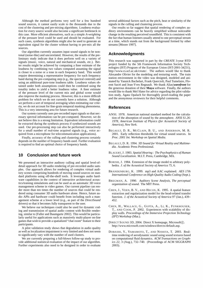
Music Voice Trainstation

cluster rng with graphics w/o graphics bothcluster rng avg. min. max. cluster rng avg. min. max. avg. min. max. avg. min. max. avg. min. max.

1 to 4 1.625 -2 4 1 to 8 1.01 -1 3 1 to 8 0.37 0 2 0.35 -1 3 0.36 -1 35 to 7 0.433 -1 3 9 to 16 0.7 0 3 9 to 16 0.011 -1 1 0.25 0 2 0.189 -1 28 to 10 0.35 -1 3 17 to 24 0.875 0 2 17 to 24 0.364 -0.1 2 0.1 -1 1 0.281 -1 2

11 to 13 0.53 -1 3 25 to 32 0.6 -1 3 25 to 32 0.34 -0.1 2 0.5 0 2 0.42 -0.1 214 to 16 0.59 -1 3 33 to 40 0.65 0 3 33 to 40 1.1 -1 4 -0.05 -1 2 0.625 -1 4

Table 3: Statistics for Reference minus Stimulus marks for the Music, Voice and Trainstation environments (negative values correspond tocases where the hidden reference received a lower mark than the actual test stimulus).

8.3 Transparency of clustering and culling

The second set of experiments aimed at evaluating the transparencyof the combined clustering and culling algorithms on the perceivedsound quality.

We used the ITU-R2 recommended triple stimulus, double blindwith hidden reference technique, previously used for quality assess-ment of low bit-rate audio codecs [Grewin 1993]. Subjects werepresented with three stimuli, R, A and B, corresponding to the ref-erence, the test stimulus and a hidden reference stimulus3. Thereference solution was a rendering with a single source per clusterand masking disabled.

Subjects could switch between the three stimuli at any time dur-ing the test by pressing the corresponding keys on the keyboard.The reproduction level could also be slightly adjusted around thecalibrated listening level until the subject felt comfortable. Subjectswere asked to rate differences between each test stimuli (A and B)and the reference R from ”imperceptible” to ”very annoying”, usinga scale from 5.0 to 1.0 (with one decimal) [ITU-R 1994].

We used two test environments, featuring different stimulustypes. In the first environment (Music) the stimulus was a 16-trackmusic signal where each track was rendered from a different loca-tion. The locations of the sources were randomized across tests.The second environment (Voice) featured a single source with aspeech stimulus but also included the 39 first specular reflectionsfrom the walls of the environment (a simple shoebox-shaped room).The location of the primary sound source was also randomizedacross tests.

As before, each subject performed each test five successive timeswith a variable number of clusters ranging from small to large. Thenumber of clusters was determined randomly for every test.

On average, 63% of the signals were masked during the sim-ulation for the Music environment and 33% of the sources weremasked in the Voice case. Table 3 reports detailed Reference minusStimulus marks averaged over five cluster ranges. Our algorithmwas rated 4.4 on average over all tests, very close to the referenceaccording to our subjects (a mark of 4.0 corresponded to ”differenceis perceptible but not annoying” on our scale). This result confirmsour hypothesis that our approach primarily trades spatial accuracyand number of sources for computing time while maintaining highrestitution quality. For very low cluster budgets (typically 1 to 4)however, significant differences were reported, especially in theMusic experiment. In such cases cluster locations can vary a lotfrom frame to frame in an attempt to best-fit the instruments withhigher loudness values, resulting in an annoying sensation.

The room acoustics application, while being very well suited toour algorithms, is also very challenging since incorrectly cullingimage-sources might introduce noticeable changes in the level, tim-bre or perceived duration of the reverberation. Based on the resultsof our experiments, our algorithms were found to perform well at

2International Telecommunication Union3i.e., the subjects did do not know which of A or B was the actual test or

the reference.

preserving the spatial and timbral characteristics of the reverbera-tion in the Voice experiment. Our other room-acoustic test (busyoffice, shown in the video) confirms that our algorithm can auto-matically cull inaudible image-sources while largely preserving theauditory qualities of the reverberation.

Influence of visual rendering

We also attempted to evaluate the influence of possible interactionbetween image and sound rendering on the quality judgment of ourperceptual audio rendering.

We repeated the above quality evaluation test using audio onlyand audio-visual presentation. Half of our subjects performed thetest with visuals and half without. The test environment was a morecomplex train station environment featuring 120 sources (see video)and we had to limit our maximum number of clusters to 40 to main-tain a good visual refresh rate.

Interestingly, the train station example received significantly bet-ter marks than the two other examples (see Table 3). This is prob-ably due to its auditory complexity since it contains many simulta-neous events, making it harder for the user to focus on a particularproblem. For this test-case, the number of subjects was not highenough for a statistical validation of our results. Nonetheless, wenote that the obtained marks are lower in the case where visualswere added. This is somewhat counter-intuitive since one could ex-pect that the ventriloquism effect4 would have helped the subjectscompensate for any spatial audio rendering discrepancy [Vroomenand de Gelder 2004]. Actually, addition of graphics may havemade it easier for the subjects to focus on discrepancies betweenthe audio and visual rendering quality. In particular, some of oursubjects specifically complained about having trouble associatingvoices with the pedestrians. We believe that our simple visual rep-resentation of the pedestrians (limited number of models, no facialanimation) failed in this case to provide the necessary visual cues toachieve proper cross-modal integration of the voice and faces whichis a situation we are highly sensitive to.

This indicates that a cross-modal importance metric should prob-ably be used, possibly increasing the importance of visible sources(as suggested by [Fouad et al. 1997]) and that care should be takenin providing a sufficiently high degree of visual fidelity to avoiddisturbing effects in cross-modal experiments.

9 Limitations of our approach

Based on this preliminary user study, our approach seemsvery promising although the tests were conducted using non-individualized binaural rendering. Using the test subjects’ ownmeasured HRTFs might reveal significant differences.

4“presenting synchronous auditory and visual information in slightlyseparate locations creates the illusion that the location of the sound is shiftedin the direction of the visual stimulus” [Vroomen and de Gelder 2004].

Although the method performs very well for a few hundredsound sources, it cannot easily scale to the thousands due to thecost of the clustering and pre-mixing algorithms. Loudness evalua-tion for every source would also become a significant bottleneck inthis case. More efficient alternatives, such as a simple A-weightingof the pressure level could be used and should be evaluated. Forsuch cases, synthesis algorithms might also be used to generate anequivalent signal for the cluster without having to pre-mix all thesources.

Our algorithm currently assumes input sound signals to be non-tonal (noise-like) and uncorrelated. However, the results of the pre-liminary study indicate that it does perform well on a variety ofsignals (music, voice, natural and mechanical sounds, etc.). Bet-ter results might be achieved by computing a finer estimate of theloudness by combining two values computed assuming the signalis closer to a noise or a tone in each frequency band. This wouldrequire determining a representative frequency for each frequencyband during the pre-computing step (e.g., the spectral centroid) andusing an additional pure-tone loudness table. Loudness values ob-tained under both assumptions could then be combined using thetonality index to yield a better loudness value. A finer estimateof the pressure level of the current mix and global scene wouldalso improve the masking process. However, this is a more difficultproblem for which we do not currently have a solution. Althoughwe perform a sort of temporal averaging when estimating our crite-ria, we do not account for fine-grain temporal masking phenomena.This is a very interesting area for future research.

Our system currently uses pre-recorded input signals so that nec-essary spectral information can be pre-computed. However, we donot believe this is a strong limitation. Equivalent information couldbe extracted during the synthesis process if synthesized sounds areused. Our pre-processing step can also be performed interactivelyfor a small number of real-time acquired signals (e.g., voice ac-quired from a microphone for telecommunication applications).

Finally, accuracy of the culling and clustering process certainlydepends on the number of frequency bands used. Further evaluationis required to find an optimal choice of frequency bands.

10 Conclusion and future work

We presented an interactive auditory culling and spatial level-of-detail approach for 3D audio rendering of pre-recorded audio sam-ples. Our approach allows for rendering of complex virtual audi-tory scenes comprising hundreds of moving sound sources on stan-dard platforms using off-the-shelf tools. It leverages audio hard-ware capabilities in the context of interactive architectural acous-tics/training simulations and can be used as an automatic 3D voicemanagement scheme in video games. Our current pipeline can ren-der more than ten times the number of sources that could be ren-dered using consumer 3D audio hardware alone. Hence, future au-dio APIs and hardware could benefit from including such a man-agement scheme at a lower level (e.g., as part of the DirectSounddrivers) so that it becomes fully transparent to the user.

We believe our techniques could also be used for dynamic cod-ing and transmission of spatial audio content with flexible render-ing, similar to [Faller and Baumgarte 2002]. This would be particu-larly useful for applications such as massively multi-player on-linegames that wish to provide a spatialized “chat room“ feature to theirparticipants.

A pilot validation study shows that degradation in audio qualityas well as localization impairment is very limited and does not seemto significantly vary with the number of used clusters.

We are currently preparing a full-blown follow-up study to pro-vide additional statistical evaluation of the impact of our algorithm.Further experiments also need to be designed in order to evaluate

several additional factors such as the pitch, beat or similarity of thesignals in the culling and clustering process.

Our results so far suggest that spatial rendering of complex au-ditory environments can be heavily simplified without noticeablechange in the resulting perceived soundfield. This is consistent withthe fact that human listeners usually attend to one perceptual streamat a time, which stands out from the background formed by otherstreams [Moore 1997].

Acknowledgments

This research was supported in part by the CREATE 3-year RTDproject funded by the 5th Framework Information Society Tech-nologies (IST) Program of the European Union (IST-2001-34231),http://www.cs.ucl.ac.uk/create/. The authors would like to thankAlexandre Olivier for the modeling and texturing work. The trainstation environment in the video was designed, modeled and ani-mated by Yannick Bachelart, Frank Quercioli, Paul Tumelaire, Flo-rent Sacre and Jean-Yves Regnault. We thank Alias|wavefront forthe generous donation of their Maya software. Finally, the authorswould like to thank Mel Slater for advice regarding the pilot valida-tion study, Agata Opalach for thoroughly proof-reading the paperand the anonymous reviewers for their helpful comments.

References

ANSI. 1978. American national standard method for the calcula-tion of the absorption of sound by the atmosphere. ANSI S1.26-1978, American Institute of Physics (for Acoustical Society ofAmerica), New York.

BEGAULT, D. R., MCCLAIN, B. U., AND ANDERSON, M. R.2001. Early reflection thresholds for virtual sound sources. InProc. 2001 Int. Workshop on Spatial Media.

BEGAULT, D. R. 1994. 3D Sound for Virtual Reality and Multime-dia. Academic Press Professional.

BLAUERT, J. 1983. Spatial Hearing : The Psychophysics of HumanSound Localization. M.I.T. Press, Cambridge, MA.

BORISH, J. 1984. Extension of the image model to arbitrary poly-hedra. J. of the Acoustical Society of America 75, 6.

BRANDENBURG, K. 1999. mp3 and AAC explained. AES 17thInternational Conference on High-Quality Audio Coding (Sept.).

BREGMAN, A. 1990. Auditory Scene Analysis, The perceptualorganization of sound. The MIT Press.

CHEN, J., VEEN, B. V., AND HECOX, K. 1995. A spatial featureextraction and regularization model for the head-related transferfunction. J. of the Acoustical Society of America 97 (Jan.), 439–452.

CHEN, H., WALLACE, G., GUPTA, A., LI, K., FUNKHOUSER,T., AND COOK, P. 2002. Experiences with scalability of dis-play walls. Proceedings of the Immersive Projection Technology(IPT) Workshop (Mar.).

DIRECT SOUND 3D, 2004. Direct X homepage, Microsoft c©.http://www.microsoft.com/windows/directx/default.asp.

DOBASHI, Y., YAMAMOTO, T., AND NISHITA, T. 2003. Real-time rendering of aerodynamic sound using sound textures basedon computational fluid dynamics. ACM Transactions on Graph-ics 22, 3 (Aug.), 732–740. (Proceedings of ACM SIGGRAPH2003).

EAX, 2004. Environmental audio extensions 4.0, Creative c©.http://www.soundblaster.com/eaudio.

ELLIS, D. 1992. A perceptual representation of audio. Master’sthesis, Massachusets Institute of Technology.

FALLER, C., AND BAUMGARTE, F. 2002. Binaural cue codingapplied to audio compression with flexible rendering. In Proc.113th AES Convention.

FILIPANITS, F. 1994. Design and implementation of an aural-ization system with a spectrum-based temporal processing opti-mization. Master thesis, Univ. of Miami.

FOUAD, H., HAHN, J., AND BALLAS, J. 1997. Perceptually basedscheduling algorithms for real-time synthesis of complex sonicenvironments. proceedings of the 1997 International Conferenceon Auditory Display (ICAD’97), Xerox Palo Alto Research Cen-ter, Palo Alto, USA.

FOUAD, H., BALLAS, J., AND BROCK, D. 2000. An extensibletoolkit for creating virtual sonic environments. Proceedings ofIntl. Conf. on Auditory Display (Atlanta, USA, May 2000).

FUNKHOUSER, T., AND SEQUIN, C. 1993. Adaptive display al-gorithms for interactive frame rates during visualization of com-plex virtual environments. Computer Graphics (SIGGRAPH ‘93proceedings), Los Angeles, CA (August), 247–254.

FUNKHOUSER, T., MIN, P., AND CARLBOM, I. 1999. Real-timeacoustic modeling for distributed virtual environments. ACMComputer Graphics, SIGGRAPH’99 Proceedings (Aug.), 365–374.

GARDNER, W. 1997. Reverberation algorithms. In Applications ofDigital Signal Processing to Audio and Acoustics, M. Kahrs andK. Brandenburg, Eds. Kluwer Academic Publishers, 85–131.

GREWIN, C. 1993. Methods for quality assessment of low bit-rateaudio codecs. proceedings of the 12th AES conference, 97–107.

HERDER, J. 1999. Optimization of sound spatialization resourcemanagement through clustering. The Journal of Three Dimen-sional Images, 3D-Forum Society 13, 3 (Sept.), 59–65.

HERDER, J. 1999. Visualization of a clustering algorithm of soundsources based on localization errors. The Journal of Three Di-mensional Images, 3D-Forum Society 13, 3 (Sept.), 66–70.

HOCHBAUM, D. S., AND SCHMOYS, D. B. 1985. A best possibleheuristic for the k-center problem. Mathematics of OperationsResearch 10, 2 (May), 180–184.

ITU-R. 1994. Methods for subjective assessment of small impair-ments in audio systems including multichannel sound systems,ITU-R BS 1116.

LAGRANGE, M., AND MARCHAND, S. 2001. Real-time addi-tive synthesis of sound by taking advantage of psychoacoustics.In Proceedings of the COST G-6 Conference on Digital AudioEffects (DAFX-01), Limerick, Ireland, December 6-8.

LARSSON, P., VASTFJALL, D., AND KLEINER, M. 2002. Betterpresence and performance in virtual environments by improvedbinaural sound rendering. proceedings of the AES 22nd Intl.Conf. on virtual, synthetic and entertainment audio, Espoo, Fin-land (June), 31–38.

LIKAS, A., VLASSIS, N., AND VERBEEK, J. 2003. The globalk-means clustering algorithm. Pattern Recognition 36, 2, 451–461.

LOKKI, T., GROHN, M., SAVIOJA, L., AND TAKALA, T. 2000.A case study of auditory navigation in virtual acoustic en-vironments. Proceedings of Intl. Conf. on Auditory Display(ICAD2000).

MARTENS, W. 1987. Principal components analysis and resynthe-sis of spectral cues to perceived direction. In Proc. Int. ComputerMusic Conf. (ICMC’87), 274–281.

MOORE, B. C. J., GLASBERG, B., AND BAER, T. 1997. A modelfor the prediction of thresholds, loudness and partial loudness. J.of the Audio Engineering Society 45, 4, 224–240. Software avail-able at http://hearing.psychol.cam.ac.uk/Demos/demos.html.

MOORE, B. C. 1997. An introduction to the psychology of hearing.Academic Press, 4th edition.

PAINTER, E. M., AND SPANIAS, A. S. 1997. A review of algo-rithms for perceptual coding of digital audio signals. DSP-97.

PAQUETTE, E., POULIN, P., AND DRETTAKIS, G. 1998. A lighthierarchy for fast rendering of scenes with many lights. Proceed-ings of EUROGRAPHICS’98.

PIERCE, A. 1984. Acoustics. An introduction to its physical princi-ples and applications. 3rd edition, American Institute of Physics.

SAVIOJA, L., HUOPANIEMI, J., LOKKI, T., AND VAANANEN, R.1999. Creating interactive virtual acoustic environments. J. ofthe Audio Engineering Society 47, 9 (Sept.), 675–705.

SENSAURA, 2001. ZoomFX, MacroFX, Sensaura c©.http://www.sensaura.co.uk.

SOUNDBLASTER, 2004. Creative Labs Soundblaster c©.http://www.soundblaster.com.

STEIGLITZ, K. 1996. A DSP Primer with applications to digitalaudio and computer music. Addison Wesley.

TSINGOS, N., AND GASCUEL, J.-D. 1997. Soundtracks for com-puter animation: sound rendering in dynamic environments withocclusions. Proceedings of Graphics Interface’97 (May), 9–16.

TSINGOS, N., FUNKHOUSER, T., NGAN, A., AND CARLBOM,I. 2001. Modeling acoustics in virtual environments using theuniform theory of diffraction. ACM Computer Graphics, SIG-GRAPH’01 Proceedings (Aug.), 545–552.

VAN DEN DOEL, K., PAI, D. K., ADAM, T., KORTCHMAR, L.,AND PICHORA-FULLER, K. 2002. Measurements of perceptualquality of contact sound models. In Proceedings of the Inter-national Conference on Auditory Display (ICAD 2002), Kyoto,Japan, 345–349.

VAN DEN DOEL, K., KNOTT, D., AND PAI, D. K. 2004. In-teractive simulation of complex audio-visual scenes. Presence:Teleoperators and Virtual Environments 13, 1.

VROOMEN, J., AND DE GELDER, B. 2004. Perceptual effectsof cross-modal stimulation: Ventriloquism and the freezing phe-nomenon. In Handbook of multisensory processes, G. Calvert,C. Spence, and B. E. Stein, Eds. M.I.T. Press.

WENZEL, E., MILLER, J., AND ABEL, J. 2000. A software-based system for interactive spatial sound synthesis. Proceedingof ICAD 2000, Atlanta, USA (April).

ZWICKER, E., AND FASTL, H. 1999. Psychoacoustics: Facts andModels. Springer. Second Upadated Edition.