performance adaptation of gas turbines for power generation

Performance Adaptation of Gas Turbines for

Power Generation Applications

Elias Tsoutsanis

Submitted for the degree of PhD

Department of Power and Propulsion

Cran�eld University

Cran�eld, UK

2010

1

Cran�eld University

School of Engineering

PhD

2010

Elias Tsoutsanis

Performance Adaptation of Gas Turbines for

Power Generation Applications

Academic Supervisor: Dr Yi-Guang Li

Academic Advisor: Professor Pericles Pilidis

Industrial Advisor: Mr. Michael Newby

June 29, 2010

© Cran�eld University

All rights reserved. No part of this publication may be reproduced

without the written permission of the copyright holder.

2

Abstract

One of the greatest challenges that the world is facing is that of providing everyone

access to safe and clean energy supplies. Since the liberalization of the electricity

market in the UK during the 1990s many combined cycle gas turbine (CCGT) power

plants have been developed as these plants are more energy e�cient and friendlier to

the environment. The core component in a combined cycle plant is the gas turbine.

In this project the MEA's Pulrose Power Station CCGT plant is under investigation.

This plant consists of two aeroderivative LM2500+ gas turbines of General Electric for

producing a total of 84MW power in a combined cycle con�guration.

Accurate gas turbine performance simulation and adaptation leads to robust diag-

nostic analysis which saves time and money in a sector where even a percent change

in thermal e�ciency is translated to thousands of pounds. For satisfying the needs

of such a competitive environment various software capabilities have been developed

for performance and �nancial analysis of a power plant. The software that Cran�eld's

University has built for performance simulation and diagnostics is PYTHIA. This has

a graphical user interface (GUI) and performs thermodynamic calculations through the

Turbomatch code, which has an international reputation and experience of 30 years.

The limitations that, exclusive manufacturer's property, compressor maps have im-

posed at o�-design performance prediction of a gas turbine have been overcome by the

development of a novel o�-design performance adaptation method. The new approach

is capable of adapting the performance of an engine model to that of a service engine

at part load conditions. This method has been developed in visual basic and integrated

into PYTHIA's environment. The proposed adaptation method initially generates a

series of compressor maps, which in turn provide the performance of the engine model

at o�-design conditions. Thence from a family of possible solutions the best set of

compressor map coe�cients is determined through a genetic algorithm optimiser. The

genetic algorithm optimisation is based on a maximum �tness criterion between the

3

engine model simulated measurements and the target measurements of the adaptation,

which are available from the service engine.

Through a series of case studies the developed adaptation's quality and accuracy

have been validated and tested. The proposed method in conjuction with a novel

compressor map generation approach, which is integrated in the adaptation process, is

able to match very accurately the performance of a gas turbine at part load conditions.

Apart from adaptation of the engine model to a single operating point set of service

engine target data the method is able to match multiple o�-design operating points

simultaneously. The developed method's limitations, which are due to the interaction

between PYTHIA'S code and Turbomatch code, a�ect the range of operating conditions

that the adaptation can capture in a single simulation.

The new adaptation approach is a fast and accurate method for matching a gas

turbine's performance at o�-design conditions and has the prospects, after a series of

proposed modi�cations, to extend its application span to that of an engine's operating

envelope. The establishment of a robust o�-design performance adaptation method is

a fundamental contribution to knowledge in the gas turbine energy sector.

4

Acknowledgements

I would like to take this opportunity to thank and express my sincere gratitude to

Professor Pericles Pilidis for giving me the opportunity to do a research degree in a

project where I feel very fortunate to be a part of, and for his expert guidance and

support.

I am deeply indebted to my supervisor Dr. Yi-Guang Li for his constant support,

invaluable advice and constructive suggestions that greatly has enriched my knowledge

with his exceptional insights in gas turbine performance and diagnostics. His guidance

has helped me construct a robust theoretical background and he has given much time

and devotion for this project.

I also would like to thank my industrial supervisor Mr. Mike Newby for his support

and for regularly devoting much of his invaluable time in the project.

In the initial period of the project I had the pleasure to collaborate with Mr. Marco

Mucino and his challenging suggestions and motivating discussions are greatly appre-

ciated.

I would like to thank my colleagues Nikolaos Asproulis, Antony Milonas, Christos

Vamvakoulas and Dimitris Mantzalis that have been and still are an excellent compan-

ion and very good friends. I am deeply thankful to my o�ce mate doctoral researcher

Emad Hamid for all the constructive discussions and his kindness. I would also like to

acknowledge my departmental colleagues Pavlos Zachos, Dimitrios Fou�ias and Kon-

stantinos Kyprianidis with who we harmoniously shared the same corridor of the 183

building.

Thanks also to Angelos Varelis of hellenic air force for all the suggestions and discus-

sions we had through the duration of my PhD. I also have to acknowledge Panagiotis

Stathopoulos of hellenic air force and his family for their excellent companion and

friendship.

A big �thank you� goes to my parents Dimitrios and Aggeliki for their continuing

5

support and to my brother Panagiotis, who has also completed his PhD in Cran�eld

University, for his conststructive comments and suggestions. Last but not least I would

like to express my appreciation to my girlfriend Kelly for her patience and understanding

during my study.

The �nancial support provided by Manx Electricity Authority (MEA), the Engi-

neering and Physical Sciences Engineering Council (EPSRC), and Cran�eld University

is greatly acknowledged.

6

To my parents Dimitrios and Aggeliki who instill in me the drive and

determination to follow my dreams and pursue my goals.

7

Contents

1 Introduction 14

1.1 Aims and Objectives . . . . . . . . . . . . . . . . . . . . . . . . . . . . 15

1.2 Thesis Contribution . . . . . . . . . . . . . . . . . . . . . . . . . . . . . 16

1.3 Thesis Overview . . . . . . . . . . . . . . . . . . . . . . . . . . . . . . . 18

2 Combined Cycle Gas Turbines 20

2.1 Introduction . . . . . . . . . . . . . . . . . . . . . . . . . . . . . . . . . 20

2.2 MEA Power Station . . . . . . . . . . . . . . . . . . . . . . . . . . . . 21

2.3 GE LM2500+ Gas Turbine . . . . . . . . . . . . . . . . . . . . . . . . . 24

2.4 Plant's Simulation . . . . . . . . . . . . . . . . . . . . . . . . . . . . . 37

2.5 Plant's Maintenance . . . . . . . . . . . . . . . . . . . . . . . . . . . . 39

2.6 Plant's Trading Model . . . . . . . . . . . . . . . . . . . . . . . . . . . 45

2.7 Industry-University Collaboration . . . . . . . . . . . . . . . . . . . . . 48

3 Design Point Performance Adaptation 51

3.1 Introduction . . . . . . . . . . . . . . . . . . . . . . . . . . . . . . . . . 51

3.2 Methodology . . . . . . . . . . . . . . . . . . . . . . . . . . . . . . . . 52

3.3 Application . . . . . . . . . . . . . . . . . . . . . . . . . . . . . . . . . 56

4 Compressor Performance Map Generating Method 62

4.1 Introduction . . . . . . . . . . . . . . . . . . . . . . . . . . . . . . . . . 62

4.2 Methodology . . . . . . . . . . . . . . . . . . . . . . . . . . . . . . . . 65

4.2.1 Speedlines . . . . . . . . . . . . . . . . . . . . . . . . . . . . . . 65

4.2.2 E�ciency . . . . . . . . . . . . . . . . . . . . . . . . . . . . . . 71

4.3 Sensitivity analysis . . . . . . . . . . . . . . . . . . . . . . . . . . . . . 75

4.4 Demonstration . . . . . . . . . . . . . . . . . . . . . . . . . . . . . . . 81

8

5 O�-Design Performance Adaptation 85

5.1 Introduction . . . . . . . . . . . . . . . . . . . . . . . . . . . . . . . . . 85

5.1.1 Genetic Algorithms . . . . . . . . . . . . . . . . . . . . . . . . . 90

5.2 Methodology . . . . . . . . . . . . . . . . . . . . . . . . . . . . . . . . 91

5.3 Application . . . . . . . . . . . . . . . . . . . . . . . . . . . . . . . . . 96

5.4 Discussion of Results . . . . . . . . . . . . . . . . . . . . . . . . . . . . 114

6 Gas Turbine Diagnostics 122

6.1 Introduction . . . . . . . . . . . . . . . . . . . . . . . . . . . . . . . . . 122

6.1.1 Gas Turbine Diagnostic Schemes . . . . . . . . . . . . . . . . . 124

6.2 Gas Path Analysis Methodology . . . . . . . . . . . . . . . . . . . . . . 127

6.3 Application . . . . . . . . . . . . . . . . . . . . . . . . . . . . . . . . . 132

7 Conclusions and Future Recommendations 137

Bibliography 140

9

List of Figures

2.1 CCGT . . . . . . . . . . . . . . . . . . . . . . . . . . . . . . . . . . . . 22

2.2 Isle of Man Generation . . . . . . . . . . . . . . . . . . . . . . . . . . . 23

2.3 GE LM2500+ HSPT . . . . . . . . . . . . . . . . . . . . . . . . . . . . 24

2.4 Inlet . . . . . . . . . . . . . . . . . . . . . . . . . . . . . . . . . . . . . 25

2.5 Engine's Numbering system . . . . . . . . . . . . . . . . . . . . . . . . 26

2.6 LM2500+ compressor . . . . . . . . . . . . . . . . . . . . . . . . . . . . 28

2.7 LM2500+ Combustor . . . . . . . . . . . . . . . . . . . . . . . . . . . . 31

2.8 High Pressure Turbine . . . . . . . . . . . . . . . . . . . . . . . . . . . 33

2.9 High Speed Power Turbine . . . . . . . . . . . . . . . . . . . . . . . . . 35

2.10 PYTHIA's software platform graphical user interface . . . . . . . . . . 38

2.11 Compressor capacity factor for both engines [14] . . . . . . . . . . . . . 40

2.12 Normalized and corrected compressor performance parameters [14] . . . 41

2.13 Temperature spread of gas turbine [14] . . . . . . . . . . . . . . . . . . 42

2.14 Exhaust temperature pro�le of gas turbine [14] . . . . . . . . . . . . . . 43

2.15 MEA's Condition Monitoring Tool . . . . . . . . . . . . . . . . . . . . 44

2.16 eCCGT Trading Model program . . . . . . . . . . . . . . . . . . . . . 47

3.1 Linear |performance adaptation . . . . . . . . . . . . . . . . . . . . . . 53

3.2 Non-Linear performance adaptation . . . . . . . . . . . . . . . . . . . . 54

3.3 LM2500+ PYTHIA Model . . . . . . . . . . . . . . . . . . . . . . . . . 56

3.4 Design Point Adaptation Setting Window . . . . . . . . . . . . . . . . 60

3.5 Design Point Adaptation Result Window . . . . . . . . . . . . . . . . 61

4.1 Compressor Performance Map [30] . . . . . . . . . . . . . . . . . . . . . 63

4.2 lm2500 compressor map . . . . . . . . . . . . . . . . . . . . . . . . . . 65

4.3 Speedline curve at 63% rotational speed . . . . . . . . . . . . . . . . . 67

4.4 Speedline compressor performance map . . . . . . . . . . . . . . . . . . 68

10

4.5 Elliptical coe�cient a for LPC, HPC and LM2500 vs shaft speed . . . . 70

4.6 Elliptical coe�cient b for LPC, HPC and LM2500 vs shaft speed . . . 71

4.7 Typical compressor e�ciency map . . . . . . . . . . . . . . . . . . . . 72

4.8 E�ciency curve at 63% rotational speed . . . . . . . . . . . . . . . . . 73

4.9 Elliptical coe�cient a for LPC, HPC and LM2500 vs shaft speed . . . . 75

4.10 Sensitivity Analysis of Compressor Map Coe�cients . . . . . . . . . . . 76

4.11 E�ect of W1 coe�cient to the compressor map . . . . . . . . . . . . . . 78

4.12 E�ect of W2 coe�cient to the compressor map . . . . . . . . . . . . . . 79

4.13 E�ect of PR1 coe�cient to the compressor map . . . . . . . . . . . . . 80

4.14 E�ect of ETAb1 and ETAb2 coe�cients to the compressor map . . . . 80

4.15 Generated Compressor Performance Maps . . . . . . . . . . . . . . . . 83

5.1 O�-Design Scaling of Compressor Map . . . . . . . . . . . . . . . . . . 93

5.2 Multiple Operating Points O�-Design Scaling of Compressor Map . . . 94

5.3 Procedure of O�-Design Adaptation . . . . . . . . . . . . . . . . . . . 95

5.4 Prediction of Test Case 1 and 2 Measurable parameters after adaptation

vs �Real� data . . . . . . . . . . . . . . . . . . . . . . . . . . . . . . . . 98

5.5 Prediction error for Test Case 1 and 2 adapted measurements vs. �real�

data . . . . . . . . . . . . . . . . . . . . . . . . . . . . . . . . . . . . . 99


vs �Real� data . . . . . . . . . . . . . . . . . . . . . . . . . . . . . . . . 102

5.7 Prediction error for Test Case 3 and 4 adapted measurements vs. �real�

data . . . . . . . . . . . . . . . . . . . . . . . . . . . . . . . . . . . . . 103


vs MEA data . . . . . . . . . . . . . . . . . . . . . . . . . . . . . . . . 107

5.9 Prediction error for Test Case 5 and 6 adapted measurements vs. MEA

data . . . . . . . . . . . . . . . . . . . . . . . . . . . . . . . . . . . . . 108

5.10 Prediction of Test Case 7, 8 and 9 Measurable parameters after adapta-

tion vs MEA Data . . . . . . . . . . . . . . . . . . . . . . . . . . . . . 113

5.11 GA Fitness for Adaptation Test Cases . . . . . . . . . . . . . . . . . . 115

5.12 Minimum Objective Function for Adaptation Test Cases . . . . . . . . 116

5.13 Computation Time for Adaptation Test Cases . . . . . . . . . . . . . . 116

5.14 O�-Design adaptation setting and Results window . . . . . . . . . . . . 117

5.15 Compressor Performance maps before and after adaptation . . . . . . . 119

11

6.1 LM2500+ Nozzle Guide Vane degradation after 25,000hrs . . . . . . . 124

6.2 GPA diagnostic process chart . . . . . . . . . . . . . . . . . . . . . . . 131

6.3 Engine parameter deviation with and without corrections . . . . . . . . 134

6.4 Componenet Fault Cases GPA Index . . . . . . . . . . . . . . . . . . . 135

7.1 O�-Design adaptation Scaling of compressor map [39] . . . . . . . . . . 146

7.2 O�-Design Adaptation's Flow chart [39] . . . . . . . . . . . . . . . . . 148

12

List of Tables

3.2 MEA Data . . . . . . . . . . . . . . . . . . . . . . . . . . . . . . . . . . 58

3.4 Design Point Adaptation Results . . . . . . . . . . . . . . . . . . . . . 59

5.2 O�-Design Adaptation Test Cases . . . . . . . . . . . . . . . . . . . . . 88

5.4 Measurable Performance Parameters . . . . . . . . . . . . . . . . . . . 96

5.6 Test Cases 1 & 2: O�-Design Adaptation Results for �Real� data with

Developed Adaptation Method and Earlier Adaptation by Lo Gatto . . 97

5.8 Test Cases 3 & 4: O�-Design Adaptation Results for �Real� data with

Developed Adaptation Method and Earlier adaptation by Lo Gatto . . 100

5.10 Test Cases 5 & 6: O�-Design Adaptation Results for MEA data with

Developed Adaptation Method and Earlier adaptation by Lo Gatto . . 105

5.12 Test Cases 7 : O�-Design Adaptation Results for MEA data with Devel-

oped Adaptation Method . . . . . . . . . . . . . . . . . . . . . . . . . 110

5.14 Test Cases 8: O�-Design Adaptation Results for MEA data with Devel-


5.16 Test Cases 9: O�-Design Adaptation Results for MEA data with Devel-


5.18 Multiple Point O�-Design Adaptation Simulation Properties . . . . . . 114

6.2 Component Degradation Table . . . . . . . . . . . . . . . . . . . . . . . 123

6.4 Selected Instrumentation set for Diagnostic Analysis . . . . . . . . . . . 132

6.5 Measurement conditions . . . . . . . . . . . . . . . . . . . . . . . . . . 133

6.6 Fault Cases . . . . . . . . . . . . . . . . . . . . . . . . . . . . . . . . . 134

6.7 Componenet Degradation Results . . . . . . . . . . . . . . . . . . . . . 135

13

Chapter 1

Introduction

One of the greatest challenges facing humanity during the twenty-�rst century is that

of giving everyone on the planet access to safe, clean and sustainable energy supplies.

Energy demand is increasing and major improvements for higher energy e�ciency are

explored. A industrial revolution in the UK took place during the 1990s after the

liberalization of electricity generation market. During this period more energy e�cient

plants as the CCGTs have been built. A combined cycle is characteristic of a power

producing plant that employs more than one thermodynamic cycle. Combining two

or more "cycles" such as the Brayton and Rankine cycle results in improved overall

e�ciency.

The CCGT plants have a higher thermal e�ciency than old-fashioned coal plants

and in business terms are more pro�table. At the same time their emissions are far

lower than conventional coal/lignite plants therefore they are environmentally friendlier.

These plants evolved when natural gas was present, as this is the more e�cient way to

produce energy from this type of fossil fuel. The combined cycle plant works around

a gas turbine which is its core component. The MEA's power station in the Isle of

Man is such a combined cycle plant which produces 84MW of power and is using the

LM2500+ aero-derivative gas turbines of General Electric.

The major advantages of the gas turbine is its size and power to weight ratio. Even

with the latest heavy duty industrial machines capable of producing 600MW of power

in a combined cycle, the gas turbine's size remains a strong feature compared to the

old diesel engines and coal/lignite plants. There is margin for further improving the

performance and thermal e�ciency of such machines till they reach the theoretical

maximum as de�ned in Carnot cycle. As boards of directors and business corporations

14

will always pursue more e�cient �money machines� the large gas turbine manufacturers

will be addressed with the task of developing new gas turbines that in the future might

reach the aforementioned limit in an advanced CCGT con�guration.

Better performance is always required from the gas turbines. This a�ects operational

and maintenance costs which play a signi�cant role in the competitive energy market.

Minimizing these costs and ensuring that the plant is always running e�ciently is a key

ingredient for a pro�table energy plant. Under this scope various software capabilities

have been developed for performance and �nancial analysis of a CCGT plant. The soft-

ware that Cran�eld's University has built for performance simulation and diagnostics

is PYTHIA. This has a graphical user interface (GUI) and performs thermodynamic

calculations through the Turbomatch code, which has an international reputation and

experience.

The industrial gas turbines are packed with instrumentation systems for measuring

almost everything. However, there are various thermodynamic parameters that can not

be physically measured and these are mass �ow rates and turbine entry temperature

(TET) which is very high even for the latest of instrumentation sets. These parameters

are the ones that can verify the actual performance of a gas turbines. There are various

ways of estimating these, but the simulation software that combines both performance

simulation and actual assessment of engine health is the PYTHIA software which has

been integrated with performance adaptation and gas path analysis diagnostics. Perfor-

mance adaptation simulates the engine's capabilities and control logic which self-adjusts

its operation and therefore its performance by any change in operating and ambient

conditions.

The cooperating body and one of the major �nancial sponsors of this project is the

Manx Electricity Authority's (MEA) Pulrose power station in the Isle of Man. This

CCGT plant produces 84MW of power and is using the LM2500+ aero-derivative gas

turbines of General Electric.

1.1 Aims and Objectives

The aim of this research project is the development of a new version of PYTHIA software

based on the development of gas turbine performance adaptation and GPA diagnostics

that is going to be integrated to the MEA environment for easier decision making.

The project objectives are summarized here:

15

1. Using PYTHIA's software as a starting point build a LM2500+ engine model

that will have the capacity to capture accurately the performance of the MEA

gas turbines .

2. Development an o�-design adaptation method that will enable the engine model

to match the MEA's service engine performance at part load conditions.

3. Development of a gas turbine performance platform for MEA for their two existing

LM2500+ gas turbine engines implemented with fully adapted engine performance

model. The platform should provide a graphical user interface, be �exible enough

to implement varying operating conditions in performance and diagnostics analy-

sis and user friendly so that important performance parameters can be displayed

conveniently.

1.2 Thesis Contribution

The work conducted in this thesis has made signi�cant contributions to the �eld of gas

turbine performance and diagnostics for power generation applications. In particular

� A more accurate engine model of GE LM2500+, that is the prime mover of MEA's

combined cycle power plant, has been developed in Cran�eld's University perfor-

mance simulation and diagnostics software programme called PYTHIA.

� The engine model is enabled by the design point and o�-design performance adap-

tation to readapt its performance to the performance of the service engines of

MEA during the whole span of its operation.

� A novel method for generating a compressor performance map, which is a useful

performance and diagnostic tool for the whole engine, has been developed and is

capable of producing compressor maps tailored to the engine speci�cations that

an engine under investigation implies.

� An o�-design performance adaptation has been developed which employs the

compressor generating method and genetic algorithms optimisation technique for

matching the engine's model performance to the service engine of MEA at o�-

design conditions, which has enhanced the applicability of PYTHIA's simulation

and diagnostics software tool.

16

� Apart from single point adaptation the developed o�-design adaptation is able to

handle multiple operating points adaptation from a series of service engine data.

� The gas turbine diagnostics option of PYTHIA has therefore much more accurate

prediction of the engine's health at design and o�-design conditions.

� Results from this thesis have been presented in a number of international confer-

ences including the 5th International Condition Monitoritng and Machine Failure

Prevention Technology Conference, July 2008, Edinburgh, and the Gas Turbine

Conference of the Institution of Diesel and Gas Turbine Engineers, November 09,

Milton Keynes, along other key meetings and events.

A list of the papers published and the ones that are currently under preparation are

enlisted here.

1. �Gas Turbine O�-Design Performance Adaptation by Compressor Map Generation

and Genetic Algorithms Part I & II�, E.Tsoutsanis Y.G.Li P.Pilidis and M.Newby,

under preparation for journal article publication.

2. `Applied GPA diagnostics for gas turbines used in combined cycle power plants',

E.Tsoutsanis Y.G.Li M.Newby and P.Pilidis, 5th GAS TURBINE CONFER-

ENCE IDGTE, 10-11 November, 2009

3. `Industry � University Collaboration: A case study between Manx Electricity

Authority and Cran�eld University', E.Tsoutsanis M.Newby Y.G.Li and P.Pilidis,

Annual Board Meeting of the Institution of Diesel and Gas Turbine Engineers,

19th March, 2009

4. `Gas path analysis applied to an aeroderivative gas turbine used for power gener-

ation', E.Tsoutsanis Y.G.Li P.Pilidis and M.Newby, 5th International Condition

Monitoring and Machine Failure Prevention Technology, Proceedings, 15th July,

2008

5. `GPA diagnostics: an application to an industrial gas turbine', E.Tsoutsanis

Y.G.Li P.Pilidis and M.Newby, Cran�eld Multi-Strand Conference, Proceedings,

6th May, 2008,

17

1.3 Thesis Overview

This thesis is organised as follows.

Chapter 2 presents a detailed description of the combined cycle gas turbine power

plant. From the factors that drove the CCGT evolution in the early 90's up to a

description of Manx Electricity Authority Power plant at the Isle of Man are presented.

The aeroderivative gas turbine of GE the LM2500+, which is the prime mover of the

combined cycle con�guration, is analysed in terms of the function, operation and the

thermodynamics that each gas turbine component has. Finally key topics such as

gas turbine performance simulation, operation and maintenance, of the MEA's power

plant along with a brief description of the MEA-Cran�eld University's collaboration

objectives and goals during this period are presented.

Chapter 3 presents the design point performance adaptation that has been employed

in order to continuously adapt the engine model to service engine and therefore be

able to model very accurate the design point of the gas turbine. A description of

the methodology which is based on the Gas Path Analysis, similar to the GPA for

diagnostics, takes place before a simple test case application. The purpose of the test

case was to compare the performance deterioration of both gas turbines during a six

month operation period. The practical considerations of measurement corrections and

natural gas �ow recalculation enabled the design point adaptation to provide a fast and

accurate tool for assessing the performance of a gas turbine.

Chapter 4 takes over from the limitations of design point adaptation, which mo-

tivated the development of a novel compressor generation method with the ability to

improve performance adaptation at o�-design conditions. The methodology used for

this analytical process of expressing a compressor map mathematically is also presented.

The coe�cients that provide the gas turbine user with a useful guide for the shape that

a compressor map has, based on the engine's design speci�cations, are outlined. A

sensitivity analysis for the map's coe�cients also takes place. A demonstration of the

compressor generation software tool along with the algorithm and the associated steps

of calculations are presented.

Chapter 5 presents the o�-design point performance adaptation by initially outlining

the associated steps for a successful adaptation process. As long as these have been

satis�ed the methodology for this adaptation procedure at o�-design conditions becomes

an optimisation problem that genetic algorithms can handle. The relationship between

compressor map generation and the genetic algorithms has the capacity to predict

18

the performance of a gas turbine at o�-design conditions quite accurately. Several

multiple operating point test cases have been used for validating and testing the o�-

design performance adaptation against simulated and service engine data respectively.

Chapter 6 presents the gas turbine performance based diagnostics. From a general

description of the types of degradation, that an engine su�ers during its lifespan, up to

practical consideration that are a-priori required for accurate assessment of an engine's

health condition, Gas Path Analysis is the method used for this process and described in

detail. The application of this powerful diagnostic tool aims to predict the degradation

that the engine's components have experienced, in terms of performance, over a period

of three months. The �ndings of this analysis indicated that there was signi�cant

compressor fouling and negligible turbine erosion.

Chapter 7 presents the conclusions drawn from this research project and possible fu-

ture research directions in the context of gas turbine performance o�-design adaptation

and diagnostics.

19

Chapter 2

Combined Cycle Gas Turbines

2.1 Introduction

Since the early days of electricity production, power plant e�ciency has been improving

steadily. The e�ciency of a power plant is the percentage of the energy content of the

fuel input that is converted into electricity output over a given time period [1].

The most advanced form of fossil-fuel led power plant now available is the CCGT.

combined cycle power plants are more than 50% e�cient compared with the older steam

turbine power plant that is still in widespread use, where the e�ciency is only about

30%, and thus two thirds of the energy content of the input fuel is wasted in the form

of heat, usually dumped in the atmosphere via cooling towers.

CCGTs are more climate friendly than older, coal �red steam turbine plant, not

only because they are more e�cient but also because they burn natural gas, which

on combustion emits 40% less CO2, than coal per unit of energy generated [2, 3, 4].

Overall taking into account both the higher e�ciency and natural's gas lower CO2

emissions, when compared with traditional coal �red plant CCGT-based power plants

release about half as much CO2 per unit of electricity produced. Most of the reductions

that occurred in Britain's CO2 emissions during the 1990s were due to the so-called

'dash for gas' as a substitute for coal power generation.

After fuels have been converted to electricity, whether in combined cycle or steam

turbine only plant, further losses occur in the wires of transmission and distribution

systems that convey the electricity to customers. In UK these amounts to 8%. Overall

this means that even when a modern engine, high e�ciency CCGT is the electricity gen-

erator, less than half the energy in its input fuel emerges as electricity at the customers'

20

sockets. In the case of older power stations the �gure is around one-quarter.

Clearly, there is room for further improvements in the supply-side of electricity

systems, by further increasing the e�ciency of generating plant and by ensuring the

whatever waste heat remains is piped to where it can be used.

2.2 MEA Power Station

The concept of CCGT is based on the law of conservation of energy which states that

energy can not be created or destroyed, it can only be changed from one form to

another, such as when heat energy is converted to electrical energy. The power station

utilizes advanced �Combined Cycle Gas Turbine technology, based on aeroderivative

gas turbines. Air is drawn into the turbine compressor and compressed to 22barg. The

air is then passed to the combustion chamber where it mixes with natural gas or oil

fuel and the mixture is ignited. The resulting hot combustion gas rotates �rstly the

high pressure turbine that drives the compressor and then the low pressure turbine that

drives an electrical generator.

The now cooler exhaust gases then pass to the Once Through Steam Generator

(OTSG). The energy in the exhaust gas from the gas turbine is not wasted, but heats

up water inside the steam generator tubes and converts it into superheated steam. The

steam is then piped to the Steam Turbo Generator Set (ST8), which produces further

electrical power.

The spent team falls through a Condenser where cooling water cools the steam

back into water. This condensate is extracted from the condenser and pumped to the

feed-pumps, which raise the pressure su�ciently to the feedwater to be returned to the

steam generator and once more be turned into steam.

The cooling water is circulated through air cooled heat exchangers which dissipate

the energy from the condensed steam to the atmosphere. The closed circuit cooling

system does away with the vapor plume of the earlier wet cooling towers, requires less

water from the river and discharges nothing to the river.

Each gas turbine can produce 32 MW and the steam turbine 23MW giving a gross

output of 87MW. The station consumes 3MW of power for its own needs and hence

the station net output is 84MW.

21

(a) OTSG (b) Steam Generator

Figure 2.1: CCGT

The total power output is 84MW capable of satisfying the island's demand and even

exporting electricity back to the mainland UK through the cable under Irish sea.

The MEA is a statutory body charged with providing the people of the Isle of Man

with a safe, reliable and economic electricity supply. The authority has responsibility

for the generation, transmission and distribution of electricity and for the billing and

collection of revenue from these activities.

The MEA is directed by a statutory board of Tynwald. The chief executive is

responsible for the day to day functions of the authority who is supported by 4 Directors,

who are responsible for generation, network Services, corporate services and �nance.

The authority constructed an 88MW combined cycle gas turbine power station at

Pulrose in 2003 together with a natural gas pipeline from Glen Mooar to Pulrose power

station. This provides a diversity of fuel and a supply of natural gas to the island.

Power stations are situated at Pulrose, Peel, Ramsey and Sulby as seen here. Pulrose

including the CCGT has a capacity of nearly 135MW. Peel a capacity of nearly 40MW,

a diesel generating station at Ramsey with a capacity of 3.6MW, and a small hydro

station at Sulby with a capacity of 1.0MW.

22

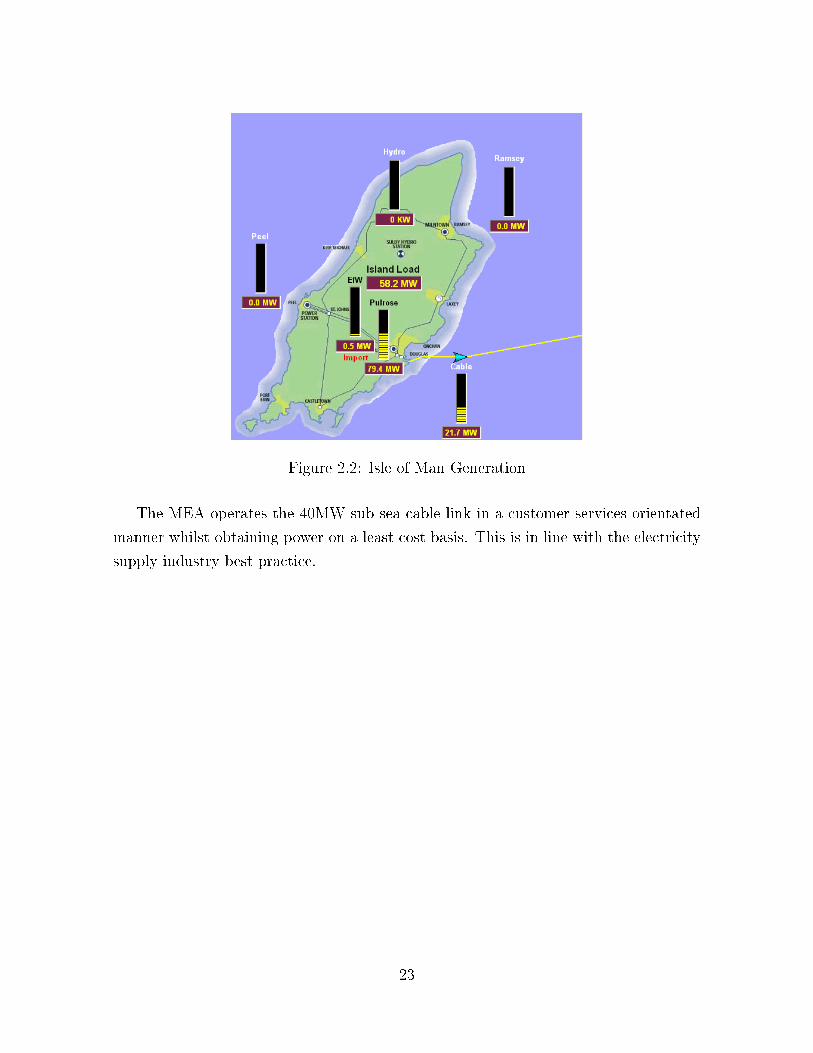
Figure 2.2: Isle of Man Generation

The MEA operates the 40MW sub sea cable link in a customer services orientated

manner whilst obtaining power on a least cost basis. This is in line with the electricity

supply industry best practice.

23

2.3 GE LM2500+ Gas Turbine

The LM2500+ is an aeroderivative gas turbine of General Electric. It is a descendant

of the CF6 family of GE aero engines modi�ed for Land and Marine applications as

LM notation stands for. While aircraft engines have multiple operating points such as

take-o�, cruise, etc, where performance is crucial, the LM2500+ is required to operate

at close to its peak e�ciency near its high-speed design point [5, 6]. The high cycle

pressure ratio achieved in the CF6-6 core results in gas generator with a high thermal

e�ciency of 39% [7].

In this case two engines are used for power generation in a CCGT power plant in

the Isle of Man. Each engine is coupled to a power turbine which delivers the power

output and therefore being the main contributor in the total power generated in the

CCGT plant.

Figure 2.3: GE LM2500+ HSPT

There are many possible con�gurations of this engine concerning the type of combus-

tor and power turbine. There are both advantages and disadvantages for each possible

con�guration and the �nal decision is up to the customer's needs and requirements.

The speci�c engines are con�gured with a single annular combustor (SAC) and with a

two stage high speed power turbine (HSPT). The main gas generator operates in the

range of 9,000rpm whereas the power turbine is coupled to this with a gearbox down to

6,100rpm at a frequency of 50Hz. It is essential at this stage to analyze each component

of the engines individually as follows.

24

Intake

Function

The primary purpose of the inlet is to bring the air required at the engine of the

compressor with minimum total pressure loss. The inlet interchanges the organized

kinetic and thermal energies of the gas in an essentially adiabatic process. The inlet

design is a very challenging aerodynamic task for designers as its property is to attract

the air by providing a minimum loss in pressure.

(a) Inlet (b) Inlet cutaway

Figure 2.4: Inlet

This temporarily satis�es the air�ow which always follows the easiest in terms of

pressure drop path (i.e. from high pressure to lower pressure) to be later compressed

and satisfy the thermodynamic cycle with a series of instant processes. Ambient air is

cleared by the air �ltration system and then guided to each engine at the enclosure. It

is then fed to the intake of the engine where the thermodynamic process begins.

Operation

The inlet guide vane (IGV) design was important because it has to deliver the required

swirl distribution to the zero stage blade at the design condition and it has to be able

to operate adequately at part speed when the airfoil is closed by as much as 60deg [7].

Thermodynamic Analysis

The numbering system used for this simple analysis can be seen here.

25

Figure 2.5: Engine's Numbering system

Following the path of the air from far upstream the air is brought to the intake. In

the thermodynamic cycle calculations the stagnation conditions are the ones required

(T0x, P0x). The total stagnation temperature at intake T01 can be calculated by:

� Obtaining the ambient static temperature Ta from the following equation:

Ma =Va√γaRaTa

(2.1)

� Assuming that Ta is equal to the static temperature at intake T1 and

� Applying the relation between static and stagnation temperatures T1, T01:

T01T1

= 1 +γ − 1

2M2

a (2.2)

The air velocity is decreased as the air is carried to the compressor inlet through the

inlet di�user and ducting system. The steady �ow energy equation (SFEE) is modi�ed

by the following assumptions:

SFEE :

q − ws = cpa(T02 − T01) (2.3)

� The process is adiabatic: q = 0

� No work done by the di�user on the �uid: ws = 0

� So equation SFEE is reduced to T02 = T01

26

That shows that the stagnation temperature at the di�user inlet T01 and that of the

compressor inlet T02 are equal. Therefore, the stagnation pressure at compressor inlet

P02 can be calculated by the temperature pressure isentropic relation.

T′02

T1=(P02

P1

) γa−1γa

(2.4)

where T′02 is the isentropic temperature at compressor inlet. State is 02

′is de�ned as

the state that would be reached by isentropic compression to the actual outlet stagnation

pressure. Since the system has losses T′02 is reduced to the stagnation temperature at

the compressor inlet T02. For the inlet di�user, an isentropic e�ciency ηd may be de�ned

as the ratio of the ideal to the actual enthalpy change during process or

ηd =h′02 − h1h02 − h1

≈ T′02 − T1T02 − T1

(2.5)

From this equation T′02 is obtained in order to use it in previous equation to �nd

P02.

27

Compressor

Function

The function of the compressor is to convert mechanical work into enthalpy as near

isentropically as possible or in other words to increase the pressure of the incoming air

so that the combustion process and power extraction process after the combustion can

be carried out more e�ciently [8]. By increasing the pressure of the air, the volume of

the air is reduced, which means that the combustion of the fuel/air mixture will occur

in a smaller volume. The compressor of this engine is a 17 stage highly sophisticated

design as seen from the �gure below.

(a) Compressor drawing

(b) Compressor cutaway

Figure 2.6: LM2500+ compressor

28

Operational

The aero performance has been obtained by measuring the inlet total pressure and

temperature by rakes mounted between strats in the forward frame. The discharge

total pressures and temperatures are measured by rakes mounted behind the OGV in

the discharge di�user [7].

The compressor has two interstage bleeds �ows for cooling purposes and these are:

1. Stage 9 bleed air for cooling the low pressure turbine and uses up to 1.5% of the

air mass �ow rate

2. Stage 13 bleed air for anti-icing, cooling the high pressure turbine and uses up to

3.3% of the air mass �ow rate

To ensure stall-free operation at part speed, the inlet guide vanes and the �rst six stators

are variable in the LM2500+. The LM2500+ uses two torque shaft assemblies located

180deg apart to actuate the compressor variable stator vanes. This con�guration has

the capability to schedule each stage with stator angle schedule that are nonlinear to

each other.

The compressor operating line was set with minimum of 12% stall margin [7]. Stall

margin is de�ned at constant corrected �ow and is:

∣∣∣∣Pstall − Po.l

Po.l

∣∣∣∣constantflow

(2.6)

A 4-deg open stator stall margin requirement was conservatively set for the LM2500+

to account for variable stator vanes (VSV) control/rigging variation and deterioration

in the �eld [7]. The schedule was checked for satisfactory aeromechanical behavior of

all blade and vane rows at all combinations of �ows and corrected speeds over a wide

range of stator angles far exceeding the control tolerance band, and over the full range

of customer bleed capabilities.


The air is compressed in the dynamic compressor so the pressure and temperature both

increase. Since the pressure increases at the compressor the SFEE is again modi�ed by

the following assumptions:

SFEE : q − ws = cpa(T03 − T02) (2.7)

29


� So equation SFEE is reduced to −ws = cpa(T03 − T02) or wc = cpa(T03 − T02)

where ws is the speci�c work done on the gas by the compressor and wc is the speci�c

work done by the compressor on the gas. The total power output from the compressor

is:

Wc = macpa(T03 − T02) (2.8)

.

The isentropic temperature at the compressor outlet T′03 can be calculated by the

isentropic temperature-pressure relation:

T′03

T02=(P03

P02

) γa−1γa

(2.9)

Again losses must be taken into consideration. a useful de�nition of an isentropic

e�ciency of the compressor ηc is the ratio of the work required in an isentropic process

to that required in the actual process, for the same stagnation pressure ratio and inlet

state:

ηc =h′03 − h02h03 − h02

≈ T′03 − T02T03 − T02

(2.10)

Also the compressor pressure ratio is de�ned as the ratio of stagnation pressure of

compressor outlet to the stagnation pressure of the compressor inlet:

Rc =P03

P02

(2.11)

combining the above two equations it is found

T′

03 = T02 (Rc)γa−1γa (2.12)

and for the isentropic e�ciency of the compressor and the compressor pressure ratio

this is

ηc =T02

(R

γa−1γa

c − 1)

T03 − T02(2.13)

30

Combustor

Function

The combustor is designed to burn a mixture of fuel and air and to deliver the resulting

gases to the turbine at a uniform temperature. The thermal energy of the fuel/air

mixture �owing through an air breathing engine is increased by the combustion process

[9, 10]. Both gas turbine engines GT6 and GT7 have a single annular combustor (SAC)

which can be seen from the �gure below. The annular combustor results in a smoother

operating line compared with the dry low emissions (DLE) combustor where the ad-

ditional air required for the combustion's processes is subtracted from the compressor

and several steps characterize its operating line.

(a) SAC drawing (b) SAC cutaway

Figure 2.7: LM2500+ Combustor

The GT6 engine and the GT7 are equipped with the G84 SAC combustor which has

dense vertical microcrack (DVM) for better Life cycle fatigue and reduction of thermal

gradient between liner and dome among a variety of advantages.


The fuel is mixed with air which supplies the oxygen for the combustion process. The

e�ciency of the burner is usually almost 100%. The equation governing the energy

balance across the burner is:

F · LHV = ma · cpp · (T04 − T03) (2.14)

31

where F is the fuel mass �ow rate.

the pressure drop across the burner ∆Pb which is taken into account is de�ned as :

∆Pb =P04 − P03

P04

(2.15)

The total power released by the combustor is:

Wb = (ma) · cpp(T04 − T03) (2.16)

32

Turbine

Function

The function of a turbine is exactly the opposite of that of a compressor. The objective

in a turbine is to convert enthalpy into mechanical work as isentropically as possible.

The turbine extracts kinetic energy from the expanding gases which �ow from the

combustion chamber [8]. The kinetic energy is converted to shaft horsepower to drive

the compressor and the accessories.

(a) Cutaway (b) HPTurbine

Figure 2.8: High Pressure Turbine

The speci�c engine has a two stage high pressure turbine (HPT) with nozzle guide

33

vanes (NGV). Whereas compressor e�ciency represents the advances in aerodynamic

design the turbine's e�ciency illustrates the advances in used material.


Since the pressure decreases at the turbine the SFEE is again modi�ed by the following

assumption:

SFEE : q − ws = cpp(T05 − T04) (2.17)


� So equation SFEE is reduced to −ws = cpp(T05 − T04) or wt = cpp(T05 − T04)

where ws is the speci�c work done on the gas by the turbine and wt is the speci�c work

done by the turbine on the gas. The total power output from the turbine is:

Wt = (ma +mf )cpp(T05 − T04) (2.18)



T′05

T04=(P05

P04

) γp−1

γp

(2.19)

Losses must be taken into consideration. The isentropic e�ciency of the turbine,

which is the ratio of actual turbine work to that which would be obtained during an

isentropic expansion to the same exhaust stagnation pressure is de�ned as:

ηt =h04 − h05h04 − h

′05

≈ T04 − T05T04 − T

′05

(2.20)

Also the turbine pressure ratio is de�ned as the ratio of stagnation pressure of

turbine inlet to the stagnation pressure of the turbine outlet:

Rt =P04

P05

(2.21)


T′

05 = T04 (Rt)γp−1

γp (2.22)

34

and for the isentropic e�ciency of the turbine and the turbine pressure ratio this is

ηt =T04 − T05

T04

(1−

(1Rt

) γp−1

γp

) (2.23)

Power Turbine

Function

The combined cycle power plant of MEA uses a freepower turbine of Nuovo Pignone

coupled to each of the gas turbines. In this arrangement the high pressure turbine

drives the compressor and the combination acts as a gas generator for the low pressure

power turbine. Several successful jet engines have been converted to shaft power use

by substituting a free power turbine for the propelling nozzle. The gas generator is

matched to the power turbine by the fact that the mass �ow leaving the gas generator

must equal that at entry to the power turbine, coupled with the fact that the pressure

ratio available to the power turbine is �xed by the compressor and the gas generator

turbine pressure ratio.

(a) Gas generator and Power turbine (b) Power turbine

Figure 2.9: High Speed Power Turbine

Each gas generator is coupled to a two stage HSPT which rotates at 6100rpm and

produces 30MW of power.

35


Since the pressure decreases at the turbine the SFEE is again modi�ed by the following

assumption:

SFEE : q − ws = cpp(T06 − T05) (2.24)


� So equation SFEE is reduced to −ws = cpp(T06 − T05) or wPT = cpp(T06 − T05)

where ws is the speci�c work done on the gas by the power turbine and wt is the speci�c

work done by the turbine on the gas. The total power output from the compressor is:

WPT = (ma +mf )cpp(T06 − T05) (2.25)



T′06

T05=(P06

P05

) γp−1

γp

(2.26)

Losses must be taken into consideration. The isentropic e�ciency of the power

turbine, which is the ratio of actual turbine work to that which would be obtained

during an isentropic expansion to the same exhaust stagnation pressure is de�ned as:

ηPT =h05 − h06h05 − h

′06

≈ T05 − T06T05 − T

′06

(2.27)

Also the power turbine pressure ratio is de�ned as the ratio of stagnation pressure

of power turbine inlet to the stagnation pressure of the power turbine outlet:

RPT =P05

P06

(2.28)


T′

06 = T05 (RPT )γp−1

γp (2.29)

and for the isentropic e�ciency of the turbine and the turbine pressure ratio this is

36

ηPT =T05 − T06

T05

(1−

(1

RPT

) γp−1

γp

) (2.30)

The useful work of this cycle is:

UW = (ma +mf )cpp (T05 − T06) (2.31)

The thermal e�ciency of this thermodynamic cycle is:

ηth =UW

HI× 100% (2.32)

2.4 Plant's Simulation

The gas turbine performance a�ects operational and maintenance costs which play a

signi�cant role in the competitive energy market. Minimizing these costs and ensuring

the plant always running e�ciently is a key ingredient for a pro�table energy plant.

Under this scope various software capabilities have been developed for performance

and �nancial analysis of a CCGT plant. Some of the most acclaimed existing programs

are enlisted here:

1. EcoSim Pro is an object-oriented simulation tool designed through FEA and CFD

performance component analysis.

2. Gas Turb commercial software which is built on Borland Delphi

3. GSP which is built by NLR on Borland Deplhi and makes full use of object

oriented features

4. ONYX is Java based and distributed through CORBA at Toledo University

5. NPSS developed by NASA which has open and extensible architecture, interface

at C++ like language, geometry computing at fortran and deploying simulation

at a computing layer

6. TURBOMATCH Object Oriented program developed in Fortran

7. PYTHIA diagnostic program based on TURBOMATCH source code for diagnos-

tics.

37

8. Other in house customised programs developed by gas turbine manufacturers.

Object orientation provides an e�cient means to implement functionality common to

the di�erent modelling elements in a simulation environment [11]. The inheritance prin-

ciple of object orientation enables the introduction of additional gas turbine component

model capabilities in a single �ancestor� component model class. The basic element is

the object: a reusable, self contained entity that consists of both data and methods to

manipulate data. An object can be assessed (by other objects) only through its external

interface. Consequently, its internal (private) data and methods are hidden (encapsu-

lated) from the other objects. Simulation of gas turbine's thermodynamic performance

is governed by the fundamental laws enlisted here.

1. Mass Conservation

2. Conservation of Momentum

3. Conservation of Energy

PYTHIA software, which has an interface built in Microsoft's Visual Basic 6.0 and

uses the fortran developed turbomatch performance code for calculations, has been

extensively used for performance simulations and diagnostics. PYTHIA's software pro-

gramme, which has a graphical user interface is seen in �gure 2.10, is a user friendly tool

that has been used from postgraduate students, researchers and industrial partners.

Figure 2.10: PYTHIA's software platform graphical user interface

38

At the start of the project the project team developed an initial model of the

LM2500+ engine, based upon the published literature about the engine. The initial

model was quite simple, utilising a single compressor element, no air bleeds and no

variable geometry capability. The model operated only with liquid fuel and had no fa-

cility for water injection. This model could thus only produce generally representative

simulated data, near to the design point of the engine when run on liquid fuel.

During this period service engine data were collated that allowed the performance

models to be progressively re�ned. This so called re�nement has been facilitated by the

application of performance adaptation [6]; a method which enables the engine model

to adapt its performance to the service engine data measurements. In addition to the

performance adaptation itself the developed engine model includes variable geometry

compressors, bleed cooling �ows, multi-fuel capability and water injection through the

combustion chamber. The engine performance models are regularly updated with the

data of MEA for accurate performance prediction and diagnostic analysis.

The software developed by gas turbine manufacturers provide useful tools to the gas

turbine users, however the expenses of such services are considerable high. Cran�eld's

diagnostics software PYTHIA with the use of turbomatch simulation code has the

capacity to facilitate the diagnostic analysis and aid the gas turbine user towards the

successful maintenance strategy of the power plant. There is still ongoing research and

development that will establish PYTHIA as a robust commercial attractive software

for performance simulation and real time diagnostics tool.

2.5 Plant's Maintenance

As a result of rising energy costs, users of individual gas turbines are seeking ways of

reducing operating costs [12]. It is essential to develop maintenance schedules based on

the characteristics of the engine and is operating environment and/or cycle in order to

balance the maintenance costs with lost revenue and extra fuel costs [4, 13]. The gas

turbine's hot gas path parts have a relative short lifespan of 4 to 8 years depending

on overall condition. In addition these parts are used under hard conditions-high �ow

rates, hot gases and frequent changes that occur during startup and shutdown. Oftenly

su�er degradation damage such as cracking, creeping and corrosion. Such damage is

tolerated in these hot gas path parts unlike steam turbine.

Currently software systems are responsible for real time online diagnostic analy-

39

sis. The MEA power station condition monitoring systems enables them to have a

continuous assessment of the power plant's performance and prompts the gas turbine

user to take action when it is required. The MEA's maintenance division schedule in-

cludes compressor washing and replacement of inlet �lters among other corrective based

maintenance actions.

Compressor Washing

One method to reduce the maintenance costs by decreasing the degradation rate and

improving the e�ciency of the powerplant is to wash the compressor both online and

o�-line. In online wash, distilled water is injected into the compressor while the gas

turbine is running such that water droplets impact the blades at high speeds to loosen

and partially remove deposits. However complete performance recovery can be achieved

by o�-line wash where distilled water (sometimes mixed with a special detergent) is

sprayed into the gas turbine while being isolated by the started at the crank speed [14].

As indicated by gas turbine manufacturer's point of view which also operates a

power station [14], in order assess the e�ectiveness of online washes with distilled water

only in a Frame 7 GE engine, trends on the capacity factor for both engines shown here

indicate several facts.

Figure 2.11: Compressor capacity factor for both engines [14]

40

� for both units engine degradation progresses at a rate of roughly one percent a

month.

� after about 2months engine degradation stabilized at the level of two percent

� there was two discernible bene�ts associated with using detergent in on-line

washes as opposed to using distilled water online

� there was a constant one percent di�erence between units A and B although both

engines were identical

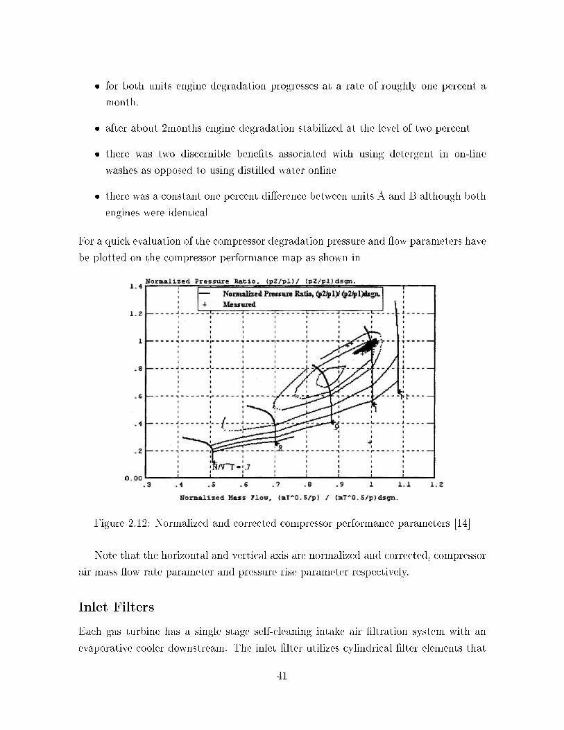
For a quick evaluation of the compressor degradation pressure and �ow parameters have

be plotted on the compressor performance map as shown in

Figure 2.12: Normalized and corrected compressor performance parameters [14]

Note that the horizontal and vertical axis are normalized and corrected, compressor

air mass �ow rate parameter and pressure rise parameter respectively.

Inlet Filters

Each gas turbine has a single stage self-cleaning intake air �ltration system with an

evaporative cooler downstream. The inlet �lter utilizes cylindrical �lter elements that

41

are sequentially cleaned by reverse �ow pulses of compressed air. A performance degra-

dation of roughly 25KW per month due to inlet �lter clogging has been presented by

Gulen [14]. Balancing the e�ects of both performance changes with the cost of �lter re-

placement, a �lter replacement date of 3 years from the last replacement date has been

predicted. However samples of �lter units revealed that they were deteriorated to the

point of performing below minimum �lter speci�cations. This demonstrates that the

pressure drop by itself is not a su�cient criterion to determine inlet �lter performance

degradation which prompts the gas turbine power plants to follow an economic based

maintenance.

Hot End Components

An important diagnostic parameter that is calculated by the monitoring software is

the ratio of the maximum exhaust thermocouple reading to the average of all exhaust

temperature thermocouple known as the temperature spread. The plot of the di�erence

between the two thermocouples i.e. the spread, shows a clear upward trend in the next

�gures [14].

(a) Exhaust temperature pro�le for engine's turbine

Figure 2.13: Temperature spread of gas turbine [14]

42

(a) Exhaust temperature spread

Figure 2.14: Exhaust temperature pro�le of gas turbine [14]

An important performance degradation source can be the combustor problems.

Most gas turbine controllers are able to detect and discard bad thermocouple read-

ings to generate a relative control signal. However, if the individual deviations (due

to possible combustor problems) are not excessive, the resulting bias of a few degrees

can still result in signi�cant loss of output. This identifying and continuously trend-

ing exhaust thermocouple spread can pinpoint problems resulting from presently mild

deviations that can lead to potentially serious engine problems or result in lost revenue.

A combustor inspection is required when this spread reaches a value of 70deg as

suggested by GE [14]. An important performance degradation source can be the com-

bustor problems. Most gas turbine controllers such as GE's Speedtronic Mark IV are

able to detect and discard bad thermocouple readings to generate a relative control

signal. However, if the individual deviations (due to possible combustor problems) are

not excessive, the resulting bias of a few degrees can still result in signi�cant loss of

output. This identifying and continuously trending exhaust thermocouple spread can

pinpoint problems resulting from presently mild deviations that can lead to potentially

serious engine problems or result in lost revenue.

43

Condition Monitoring

The performance based Gas Path Analysis has been applied to the PYTHIA's developed

engine model, for assessing the health of each gas turbine at regular time intervals and

improving the plant's availability. An application of this approach for an operation

period of three months along with the �ndings of the degraded components, measured

by the GPA Index, has been produced [15, 16] . This diagnostic analysis o�ers a

great potential to improve plant economics. The condition monitoring process has been

enhanced by reviewing the instrumentation systems, use redundant set of measurements

located in the gas path of the gas turbine and apply the appropriate corrections for

reducing repeated uncertainties like measurement noise and varying ambient conditions.

Therefore the current condition monitoring system provides a clear view of the gas

turbine performance. Real time trends of the fundamental performance parameters

monitored are available to the gas turbine user as seen in �gure 2.15.

Figure 2.15: MEA's Condition Monitoring Tool

44

CCGT Performance Modeling

The combined cycle performance analysis, which is monitored by MEA, includes the

performance simulation of the two gas turbines, two OTSG and the Steam turbine. The

CCGT performance simulation program was created from the integration of existing

and new individual performance simulation codes of the main components of a CCGT

power station using the Visual Basic for Applications (VBA) in Excel [2]. In the case of

the steam cycle, an initial model for a double pressure OTSG was produced by Mucino

[2]. A novel approach using theoretical thermohydraulic models for heat exchangers and

empiric correlations delivered positive results. Steamomatch, another code developed

at the university, was used for the combined cycle performance simulation [2]. Exten-

sive research is still being carried out for further improving the CCGT performance

simulation program by developing a series of novel simulation techniques. This enables

the project team to acknowledge the complexity involved with optimising the operation

of the CCGT by taking into consideration the limitations that each component implies

through this con�guration.

2.6 Plant's Trading Model

Since the electricity market liberalization in UK, powerplant companies want to be

energy e�cient and pro�table. In such a complex and competitive energy market it is

fundamental to ensure that production of electricity is pro�table most of the plant's

operation time. An important measure which utilizes companies determine their bottom

line (pro�t) is the spark spread. The spark spread is the theoretical net income of a

gas-�red power plant from selling a unit of electricity, having bought the fuel required

to produce this unit of electricity. All other costs (operation and maintenance, capital

and other �nancial costs) must be covered from the spark spread. If the spark spread is

small on a particular day, electricity production might be delayed until a more pro�table

spread arises.

Speci�cally the amount of fuel required to generate a unit of electricity is linked

to the plant's thermal e�ciency. The heat rate, the inverse quantity of the thermal

e�ciency, hence is de�ned as the ratio between the heat input and the power output.

The �nancial industry de�nes the spark spread [17] using the operating heat rate (HR)

of the plant in MMBtu/MWh, the electricity price in ¿/MWh (Pe) and gas price in

45

¿/MMBtu (Pg) in basic expression as follows:

π = max(Pe −HR · Pg, 0) (2.33)

Practitioners in the power industry replace the heat rate with the thermal e�ciency

ηth which is a more accessible parameter calculated during the operation of the plant.

In addition, two more coe�cients representing di�erent operating marginal costs are

introduced [18]. Ce represents the costs incurred by the company in maintenance, T&D

and electricity trading to and from the network. On the other hand, Cg, correspond to

the cost related to the transport and trade of gas

π = max

([Pe − Ce]−

[Pg + Cg

ηth

], 0

)(2.34)

For the MEA, a negative spark spread would send an economic signal to import power

along the interconnector (and back-o� or resell gas) while a positive spread would

indicate that it would be pro�table to generate from the CCGT and export the surplus

to the UK through the interconnector. The following is a list of these costs, followed

by the actual expression used:

1. Actual electricity (export) price in ¿/MWh (E)

2. Cable losses and charges in ¿/MWh (C)

3. Actual gas price in p/th (G)

4. Transco's incremental variable costs between NBP and Mo�at in p/th (S)

5. Gas Interconnector (IC2) commodity charge in p/th (I)

6. CCGT variable maintenance costs in ¿/MWh (M)

7. Thermal e�ciency (T)

8. Gas price �swing� premium in p/th (P)

π = max

([E − C −M ]−

[(G+ S + I + P ) · 0.3412

ηth

], 0

)(2.35)

Computational method

46

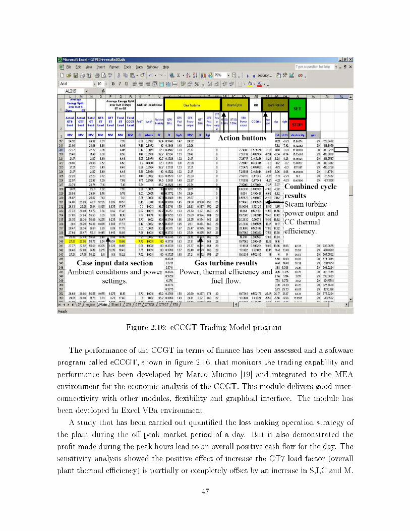
Figure 2.16: eCCGT Trading Model program

The performance of the CCGT in terms of �nance has been assessed and a software

program called eCCGT, shown in �gure 2.16, that monitors the trading capability and

performance has been developed by Marco Mucino [19] and integrated to the MEA

environment for the economic analysis of the CCGT. This module delivers good inter-

connectivity with other modules, �exibility and graphical interface. The module has

been developed in Excel VBa environment.

A study that has been carried out quanti�ed the loss making operation strategy of

the plant during the o� peak market period of a day. But it also demonstrated the

pro�t made during the peak hours lead to an overall positive cash �ow for the day. The

sensitivity analysis showed the positive e�ect of increase the GT7 load factor (overall

plant thermal e�ciency) is partially or completely o�set by an increase in S,I,C and M.

47

Whereas, the GT7 load factor has a secondary order of magnitude when the electricity

or gas prices are modi�ed [19].

A number of operations optimisation strategies, which are based on the technical

performance simulation of the plant under these speci�c conditions, have been proposed

in order to increase the pro�tability of the plant. The developed techno-economic

software eCCGT is positively a�ecting the way an operator manages a power generation

asset through the implementation of virtually proven optimisation and risk management

strategies.

2.7 Industry-University Collaboration

Detailed understanding and monitoring of power plant performance, prime mover health

condition and associated costs have a deep impact in the decision making process con-

cerning the plant's operational and maintenance strategy. In this context, research

collaboration between Manx Electricity Authority (MEA) and Cran�eld University has

been carried out since 2001 and a series of technologies and software have been and are

still being developed at Cran�eld University and some of them have been integrated into

MEA Combined Cycle Gas Turbine Power Plant in Pulrose, Isle of Man. During this

constructive and successful collaboration period, the University has been fortunate to

acknowledge the industrial needs and make signi�cant academic contributions through

ongoing research projects jointly supported by both MEA and EPSRC. On the other

hand, MEA has valued the complexity of asset management concerning the gas turbine

and the combined cycle, therefore enhancing its trading and operational capabilities

through the application of developed performance, diagnostic, trading and economic

analysis software.

The Manx Electricity Authority (MEA) is an Island based electricity generation

utility. The company undertook a massive expansion in its operations during the pe-

riod between 1999 and 2004 in response to the Isle of Man Department of Trade and

Industry's strategic objectives for the island economy at that time. As part of this

technology upgrade programme the MEA took the decision to invest in a high technol-

ogy state of the art Combined Cycle Gas Turbine (CCGT) power station in Pulrose,

Isle of Man and trade the excess output from this power station in the UK wholesale

electricity and gas markets. The design of the plant started in 2001 just after the Inter-

connector cable began its operations. Since then and as part of this process the MEA

48

has closely collaborated with the department of Power and Propulsion of Cran�eld Uni-

versity, which has established an international reputation for its advanced postgraduate

education, extensive research activity and applied continuing professional development.

A series of software programmes, which have been developed in the university, for per-

formance simulation of gas turbines, heat exchangers and steam turbines have been

integrated to MEA power station. Diagnostics tools based on the Gas Path Analysis

(GPA) method have also been used for the gas turbines. These along with the economic

and trading analysis software tools have enriched MEA's understanding and knowledge

for successful asset management of their power plant with signi�cant bene�ts for both

parties.

The objectives of this collaboration have been classi�ed in two categories: techni-

cal contribution and personnel training. The technical contribution has been achieved

through the development of new technology and new analytical tools through ongoing

academic research activities at Cran�eld University [20]. The personnel training have

been established through part-time MSc programme attended by the personnel of MEA

and PhD programme attended by PhD researchers at Cran�eld . Invited lectures at

Cran�eld provided by MEA senior managers also enhance educational programme at

Cran�eld University. The aim of this process was to enhance MEA's technical under-

standing and facilitate its decision making capability concerning the CCGT's perfor-

mance, maintenance and operations through the appropriate software tools. Some of

the technical development has already been implemented in MEA and more capabilities

are being developed at Cran�eld University and will be transferred to MEA to meet

further industrial needs.

The project team considered fundamental for this collaboration to deliver the ap-

propriate academic training to the MEA personnel through a number of seminars held

in the authority's headquarters and career development short courses attended by a

number of MEA's technical personnel. This has been essential for enhancing MEA's

knowledge and understanding for the complexity involved in operational and mainte-

nance as part of asset management skills. On the other hand the academic team, during

this period, has organised the platform for successful research activities by assigning

research projects directly related to MEA to doctoral researchers and postgraduate stu-

dents as part of their research degrees and taught postgraduate courses o�ered by the

University.

The joint research activities between Cran�eld University and MEA have resulted

in academic contributions and publications in research communities. Four conference

49

papers on gas turbine performance adaptation [21], gas turbine performance diagnostics

[22, 15, 16, 23] and gas turbine combined cycle performance [24] have been published

where one of them [21] was recommended by the conference for publication in Journal

of Engineering for Gas Turbines and Power. The academic contributions from the joint

research have been well recognized both nationally and internationally

The accomplishment of the objectives of this collaboration from the current re-

search include the development of a gas turbine software platform with fully adapted

engine models and with capability of the o� design performance adaptation. The o�

design performance adaptation enables the engine model to adapt its performance to

the service engines actual performance at part load conditions. The condition monitor-

ing system will be updated with real time on line performance and diagnostic analysis

tools provided by PYTHIA's latest version. New computer software to simulate the

performance of steam cycle at di�erent operating conditions and is adapted to real

cycle performance is under development. These software tools along with the CCGT

performance simulation system can be used in conjunction with the control systems

monitoring process at MEA for successfully managing the operations and maintenance

of MEA's CCGT power plant.

The collaboration between Manx Electricity Authority and Cran�eld University has

being constructive and successful in all the associated levels. Intense research activities

in di�erent technical and economic areas relevant to the operation and maintenance of

MEA CCGT power plant and technical training have been accomplished and are still

being carried out. Improvement in the analysis capability and understanding in gas

turbine performance, condition monitoring diagnostics, steam cycle performance and

economic trading are fundamental aspects of the collaboration's objectives. The deep

impact that quality measurement data provided by MEA have towards the validation of

the research techniques developed through the academic research has been recognized

and the e�ort made by MEA to improve the measurement quality is greatly appreciated.

MEA's personnel are able to use the developed analytical software to make an informed

judgement based on the information from both power plant measurement systems and

the analytical results from the software. The result is that assets are better managed;

the plant availability increases and maintenance and life cycle costs are signi�cantly

reduced.

50

Chapter 3

Design Point Performance Adaptation

3.1 Introduction

Accurate simulation and understanding of gas turbine performance is fundamental for

gas turbine users. A performance simulation should always start from the design point

of the engine that is modeled. When some of the engine component parameters for an

existing engine are not available, they must be estimated in order that the performance

analysis can be carried out. However, the initially simulated design point performance

of the engine using estimated engine component parameters may give a result that

is di�erent from the actual measured performance. This di�erence may be reduced

with better estimation of these unknown component parameters. However, this can be-

come a di�cult task for performance engineers, let alone those without enough engine

performance knowledge and experience, when the number of design point component

parameters and the number of measurable/target performance parameters become large

[25, 23, 26]. The gas turbine design point performance adaptation approach that has

been developed by Li [27] is used for adapting the engine model of the GE LM2500+ gas

turbine. In the approach, the initially unknown component parameters may be com-

pressor pressure ratios and e�ciencies, turbine entry temperature, turbine e�ciencies,

air mass �ow rate, cooling �ows, by-pass ratio, etc. The engine target (measurable)

performance parameters are shaft power and thermal e�ciency for industrial engines,

gas path pressures and temperatures, etc.

The adaptation procedure suggests values of performance parameters (e�ciencies,

mass �ows, TET) that would satisfy the target measurements (temperatures and pres-

sures at various locations). The success of this analysis depends on the thermodynamic

51

relationships between the performance parameters and the measurements.

3.2 Methodology

Design point performance adaptation is an inverse mathematical problem. The infor-

mation of the dependent parameters in a system is used to estimate the quantity of

the independent variables of the model as described by Li [27]. The matrix inverse

mathematical model used in the GPA approach used by Escher and Singh [28]in their

diagnostics method is an e�ective solver to model-based inverse problems and can be

applied to engine design point performance adaptation. The thermodynamic relation-

ship between gas turbine to-be-adapted component parameters and target performance

parameters of a gas turbine can be expressed with the following equation

~z = h(~x) (3.1)

where ~z ∈ <M is the target performance parameter vector andM is the number of target

performance parameters, and ~x ∈ <N is the to-be- adapted component parameter vector

and N is the number of to-be-adapted component parameters and h( ) is a vector valued

function.

At an initially given design point which is denoted with subscript �0� equation x

can be expanded in a Taylor series as:

~z = z0 +∂h(~x, ~y)

∂x· (~x− ~x0) +HOT (3.2)

HOT represent higher order terms which can be neglected. This assumption lin-

earises the relationship between the deviation of the design point to-be-adapted com-

ponent parameters and the deviation of their corresponding design point target perfor-

mance parameters of a gas turbine and can be expressed as:

∆~z = H ·∆~x (3.3)

For any expected deviation of ∆~z from its initial point, the deviation of to-be-adapted

component parameters from its initial point can be predicted by inverting the in�uence

coe�cient matrix (ICM) H to a adaptation coe�cient matrix (ACM) H−1 leading to

equation xx when N = M

∆~x = H−1 ·∆~z (3.4)

52

Figure 3.1: Linear |performance adaptation

The idea of linear adaptation is shown here where the linear prediction of ∆~x will be

a good estimate of the engine to-be-adapted component parameters from their initial

values when the shift is small and the thermodynamic behavior of the engine around

the initial design point is linear.

It is very likely that when the nonlinearity of the relationship between the to-

be-adapted component parameters and the target performance parameters is signi�-

cant, the predicted deviation of to-be-adapted components will not the same accuracy.

The nonlinearity of of the thermodynamic behavior is taken into account by using

the Newton-Raphson iterative method, Escher and Singh [28],where linear prediction

process is applied iteratively until a converged solution is obtained as seen here.

In many cases, the number of to-be-adapted component parameters N and the

number of target performance parameters N may not be equal. If N > M equation x

is under-determined and this leads to an in�nite number of least-squares solutions. A

pseudoinverse matrix is de�ned as:

H# = HT · (HHT )−1 (3.5)

53

Figure 3.2: Non-Linear performance adaptation

The solution resulting from this, which is the best in a least square sense, is:

~x = H# · ~z (3.6)

If N < M equation x is over-determined and there are redundant equations. A


H# = (HTH)−1 ·H−T (3.7)

The resulting resulting, which is also the best in a least square sense, is:

~x = H# · ~z (3.8)

The convergence of this iterative adaptation calculation process is declared when

the performance is very close to the real target performance. The root mean square

(RMS) of the di�erence between predicted and target performance is smaller than

54

σwhen convergence criterion is satis�ed.

RMS =

√∑(zi,predicted − zi,measured)2

M< σ (3.9)

where σ is a very small number (σ=0.001 is usually chosen). The adaptation error εi

for the ith performance parameter is:

εi =zi,predicted − zi,measured

zi,measured

· 100% (3.10)

For the design point adaptation procedure to be successful the compressor map has to

be scaled with the following scaling factors. The de�nition of the design point scaling

factors is shown here

SFN,DP =NDP

NDP0

= 1 (3.11)

SFPR,DP =PRDP − 1

PRDP0 − 1(3.12)

SFWAC,DP =WACDP

WACDP0

(3.13)

SFETA,DP =ETADP

ETADP0

(3.14)

where WAC is the corrected mass �ow rate, PR is the pressure ratio, ETA is the

isentropic e�ciency and N is the non-dimensional shaft rotational speed. The scaling

factors need to be applied to the whole default compressor characteristic map with the

next four equations in order to make it representative of the behavior of the compressor

of interest.

N = NDP0 (3.15)

PRDP = SFPR,DP ∗ (PRDP0 − 1) + 1 (3.16)

WACDP = SFWAC,DP ∗WACDP0 (3.17)

ETADP = SFETA,DP ∗ ETADP0 (3.18)

The scaled map compared with the old default compressor map can be seen here

Every single point is scaled by the scaling factors in order to match the new set design

point. This adaptation procedure provides excellent results for target measurements

close to the design point of the engine but cannot deliver solutions of the same accuracy

55

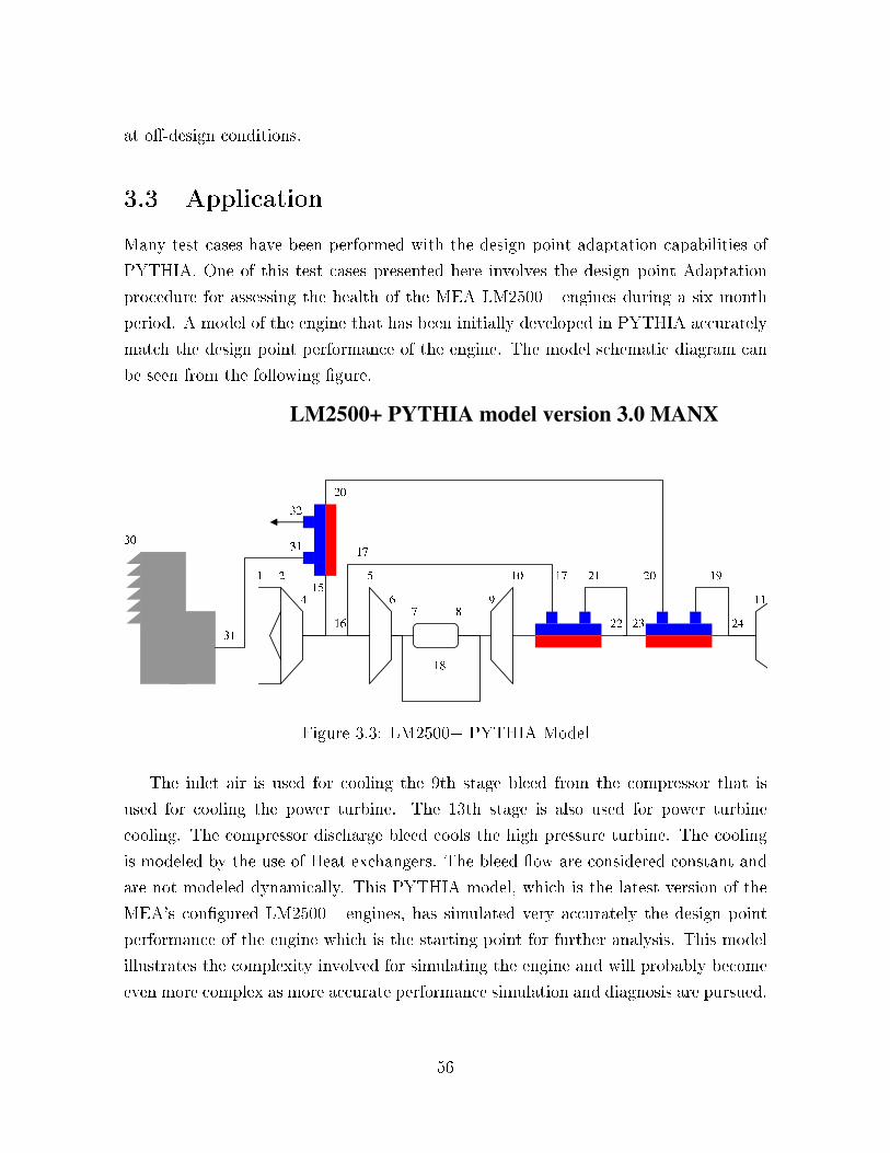
at o�-design conditions.

3.3 Application

Many test cases have been performed with the design point adaptation capabilities of

PYTHIA. One of this test cases presented here involves the design point Adaptation

procedure for assessing the health of the MEA LM2500+ engines during a six month

period. A model of the engine that has been initially developed in PYTHIA accurately

match the design point performance of the engine. The model schematic diagram can

be seen from the following �gure.

Figure 3.3: LM2500+ PYTHIA Model

The inlet air is used for cooling the 9th stage bleed from the compressor that is

used for cooling the power turbine. The 13th stage is also used for power turbine

cooling. The compressor discharge bleed cools the high pressure turbine. The cooling

is modeled by the use of Heat exchangers. The bleed �ow are considered constant and

are not modeled dynamically. This PYTHIA model, which is the latest version of the

MEA's con�gured LM2500+ engines, has simulated very accurately the design point

performance of the engine which is the starting point for further analysis. This model

illustrates the complexity involved for simulating the engine and will probably become

even more complex as more accurate performance simulation and diagnosis are pursued.

56

Engine Operating History

The GT6 engine has operated for a total amount of 19678 hours, which is 25% more

than the GT7. This simply indicates that the GT6 engine will theoretically have greater

degradation. However this is not always true since the operating hours that a gas

turbine has maintenance wise is a function of actual operating hours, number of start-

ups, trips, load dumps and peak operating hours. Considering only the fact that GT7

has experienced more start-ups than the GT6 contributes signi�cantly to the EOH

which might be equal to the GT6.

Maintenance Action

The fuel nozzles at the GT6 have been replaced back in April. This action is going to

a�ect the performance analysis as this will lead at higher combustion e�ciency.

Data analysis

Two similar power setting points have been selected for this analysis. The one from

18th of January at 06:50am and the other at the 18th of June at 11:26am for GT6.

A similar set of points has been selected for the GT7 as well. The data are tabulated

below.

57

Parameter GT6@Jan(Jun) GT7@Jan(Jun) Units

Power 28.1(28.1) 28.1(28.1) MW

Operating hours 16645(19678) 12776(15188) Hrs

Ambient Temperature 286.65(288.55) 280.65(288.45) K

Ambient Pressure 0.9716(1.0048) 0.9967(1.0048) Bar

Ambient Humidity 99.8(95.1) 88.9(95.1) %

NGG 9751(9778) 9649.5(9775) rpm

VSV Position �(9.4233) �(9.52) %

Comp. Bleed Pres. 0.9(9.2) 9.4(0.8) Bar

Comp. Bleed Temp. 420.45(423.95) 425.35(429.45) K

Comp. Discharge Pres. 21.3(21.5) 22(21.8) Bar

Comp. Discharge Temp. 757.05(758.85) 743.45(758.85) K

Turbine Exit Pressure 4.3(4.4) 4.4(4.4) Bar

Turbine Exit Temperature 1118.15(1109.15) 1085.15(1097.15) K

Exh. Temp. out of HSPT 792.75(800.35) 770.25(787.65) K

Spread 86(37) 53(51) K

Mass Flow Calculated 75(�) 78.5(�) kg/s

Fuel Flow 7571.2(7525) 7552.8(7451.8) Sm3/Hr

Thermal E�ciency 36.67(36.94) 36.71(37.21) %

Table 3.2: MEA Data

The correct thermal e�ciencies should be higher than the data that were initially

received as there is an additional calculation involved for determining the actual fuel

�ow. This is summarized below by taking into account the density of natural gas,

since the measurement of gas fuel �ow is speci�c to its properties as indicated by the

units. Natural gas density varies from 0.7kg/m3 to 0.9kg/m3 and an average value is

assumed. The natural gas supplier provides the value of this property, which has a

signi�cant impact in the e�ciency of the GT.

F =GasF low ∗Density

3600Secs=

7571.2Sm3/s ∗ 0.8kg/m3

3600= 1.6722kg/s (3.19)

The temperature spread is dramatically reduced as the fuel nozzles have been re-

placed. A published paper on real time maintenance by GE engineers described that

the company suggests relevant maintenance action when the spread exceeds the 70deg

limit. The time to reach this limit from 50deg takes about 5 to 6 months. The exhaust

temperatures of both engines have increased. This is a very important parameter that

58

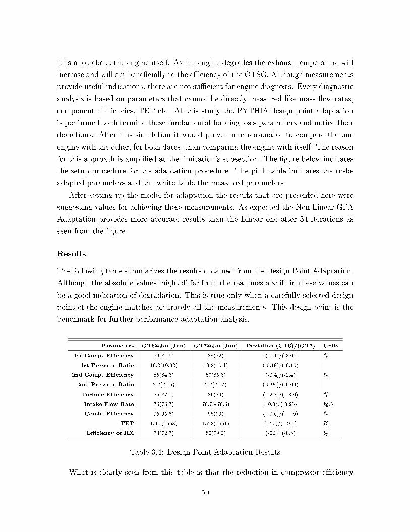
tells a lot about the engine itself. As the engine degrades the exhaust temperature will

increase and will act bene�cially to the e�ciency of the OTSG. Although measurements

provide useful indications, there are not su�cient for engine diagnosis. Every diagnostic

analysis is based on parameters that cannot be directly measured like mass �ow rates,

component e�ciencies, TET etc. At this study the PYTHIA design point adaptation

is performed to determine these fundamental for diagnosis parameters and notice their

deviations. After this simulation it would prove more reasonable to compare the one

engine with the other, for both dates, than comparing the engine with itself. The reason

for this approach is ampli�ed at the limitation's subsection. The �gure below indicates

the setup procedure for the adaptation procedure. The pink table indicates the to-be

adapted parameters and the white table the measured parameters.

After setting up the model for adaptation the results that are presented here were

suggesting values for achieving these measurements. As expected the Non Linear GPA

Adaptation provides more accurate results than the Linear one after 34 iterations as

seen from the �gure.

Results

The following table summarizes the results obtained from the Design Point Adaptation.

Although the absolute values might di�er from the real ones a shift in these values can

be a good indication of degradation. This is true only when a carefully selected design

point of the engine matches accurately all the measurements. This design point is the

benchmark for further performance adaptation analysis.

Parameters GT6@Jan(Jun) GT7@Jan(Jun) Deviation (GT6)/(GT7) Units

1st Comp. E�ciency 86(84.9) 85(82) (-1.1)/(-3.0) %

1st Pressure Ratio 10.2(10.02) 10.2(10.1) (-0.18)/(-0.10)

2nd Comp. E�ciency 85(84.6) 87(85.6) (-0.4)/(-1.4) %

2nd Pressure Ratio 2.2(2.16) 2.2(2.17) (-0.04)/(-0.03)

Turbine E�ciency 85(87.7) 86(89) (+2.7)/(+3.0) %

Intake Flow Rate 76(75.7) 78.75(78.5) (-0.3)/(-0.25) kg/s

Comb. E�ciency 95(95.6) 98(99) (+0.6)/(+1.0) %

TET 1560(1558) 1552(1561) (-2.0)/(+9.0) K

E�ciency of HX 73(72.7) 80(79.2) (-0.3)/(-0.8) %

Table 3.4: Design Point Adaptation Results

What is clearly seen from this table is that the reduction in compressor e�ciency

59

is higher in GT7 than in GT6. This might result from the di�erence in the amount of

compressor washes that each engine has experienced. The second useful conclusion is

that the combustion e�ciency has increased in GT6 because of the fuel nozzle change.

The counteracting e�ect of combustion degradation is hidden in this incremental in-

crease. The turbine e�ciency has increased as well as a consequence of the increase in

combustion e�ciency. The Power turbine e�ciencies were not involved in this analysis

as they didn't deviate because a well de�ned thermodynamically relationship with a

measurement could not be established. The performance adaptation results presented

here may be used only for a general evaluation of the engine and by no means are

eligible to provide accurate engine diagnosis which in turn might suggest the appro-

priate maintenance strategy. The setting window and results window of the o�-design

adaptation can be seen from the following �gures.

Figure 3.4: Design Point Adaptation Setting Window

60

Figure 3.5: Design Point Adaptation Result Window

In this adaptation procedure the user has no control over the other simulated mea-

surements that are not engaged for this analysis. The procedure assumes that the

engine is operating at constant speed and de�nes a new point that will match the pre-

determined engine measurements. Although this method is working accurately, and

provides very useful and meaningful conclusions, it can not be used for diagnostic anal-

ysis since speed and operating conditions change. The diagnostic analysis should be

based on accurate o�-design performance prediction which has been enhanced by the

o�-design adaptation and the compressor map generation method that are described in

the following chapters.

61

Chapter 4

Compressor Performance Map

Generating Method

4.1 Introduction

Prediction of gas turbine performance is strongly dependent on detailed understanding

of engine component behavior. For a given rotational shaft speed, there is a charac-

teristic line that describes the �ow versus pressure ratio relationship for any axial or

centrifugal compressor. This line has an upper limit that is referred to as surge point

and a lower limit that is commonly called as the choke or stonewall point. The perfor-

mance map usually also includes line of constant adiabatic e�ciency which are referred

to as e�ciency contours as seen from the �gure 4.1.

When �ow, rotational speed and compressor discharge pressure are expressed in

non dimensional terms e�ects of any changes in the compressor air inlet condition and

physical properties are eliminated. Further more, such normalized performance maps

of a variety of compressors are found to be nearly identical.

Compressor maps are based on various engine tests [29]. Shape of map helps to

determine the values of measurable parameters at o�-design operating condition. When

a speci�c target of o�-design performance is pursued then the maps must be shifted to

match the target. In order to describe the o�-design performance of gas turbine power-

plant accurately, good prediction of characteristic curves of gas turbine power-plant

components is essential. A generalized compressor map developed by Saravanamutto

and Mac Isaac [17] has been used by Zhu and Saravanamuto [18]. Kurzke [19] introduced

auxiliary coordinates (beta lines), having no physical meaning, which are superimposed

62

on the characteristic curves.

Figure 4.1: Compressor Performance Map [30]

Performance modeling of gas turbines must be established based on thermodynamic

relationships between major components in gas path and its component maps. The

compressor performance map is also a very useful diagnostic tool that lends itself to

engine performance monitoring with the most readily available measurements. When

the engine customer purchases the engine, most engine makers provide a performance

deck which can calculate only the engine performance output with input data but

cannot see the context of the program. One can construct a compressor map, from

the operational data. However this would require a reliable set of historic distributed

control system (DCS) data that is usually not the case. In generating component maps,

several methods exist and are brie�y described in this section.

A scaling method has been proposed by Kong [31] under the condition that each

engine performance must follow its own component performance. This scaling method

is applicable only if it may use similar maps to the actual engine maps which implies

63

scaling factor close to 1.0 hence similar performance behavior between original compo-

nent and scaled component. This agrees with the measured performance if the analysis

is performed near the design operating point of the engine. Another method called sys-

tem identi�cation method proposed by Kong [32] builds a math model between scaling

factors at some given conditions (input) and Pressure Ratio, Mass Flow and E�ciency

(output) with polynomial equations up to 3rd order and �nally analyzing the engine

performance with the identi�ed maps.

A di�erent approach to input output relationship for the engine/component perfor-

mance with the use of neural networks has been developed by Yu[33] through a trilinear

back propagation network. Again this method relies heavily on the quantity of engine

data from the engine manufacturer, which is not always a realistic case scenario, and

has a low precision. A combined hybrid approach developed by Kong[34] takes ad-

vantage of genetic algorithms to determine the coe�cients of the polynomial equations

of the system identi�cation method. This method provides higher accuracy than the

traditional scaling method at operating points far away from the design point of the

engine. Other approaches include fuzzy expert systems along with engine deck data for

compressor performance map estimation [35, 36]

These methods and approaches to compressor map generation techniques and their

e�ect to o�-design adaptation have limited applicability due to their case speci�c nature

which is obvious from both the consideration of engine deck data used for constructing

the performance map and by the high order polynomials which add complexity and

decrease signi�cantly the computation time.

Therefore the novel compressor performance method developed not only provides a

useful performance, adaptation and diagnostic tool but also tackles the aforementioned

issues by being generic, simpler and e�cient in terms of computation.

The aim of this method is to analyse the shape of a default compressor map math-

ematically so that this shape could then be controlled by an optimiser and therefore

match the o� design operating points of a gas turbine. The original LM2500 compressor

performance map published in [30] is taken as the default map for this analysis. This

map has been digitised from the article published by Klapproth and it can be seen in

�gure 4.1.

Each compressor map comprises of the lines of constant speed and the e�ciency

contours. The LM2500 gas turbine engine is very similar to the the LM2500+ with

their only di�erence been the zero stage at the latest version which enables the engine

to have a 23% increase in mass �ow rate. In this method the speedlines are analysed

64

�rst mathematically and then a similar analysis will follow for the e�ciency contours.

4.2 Methodology

4.2.1 Speedlines

Mathematical Analysis

The compressor map is �rst analysed by expressing the lines of constant speed in the

Pressure Ratio- Mass Flow plane as a function of the compressor's rotational speed

which is the most reliable measurement from a gas turbine instrumentation set.

Figure 4.2: lm2500 compressor map

Each speedline can be expressed by a mathematical equation. Amongst a variety of

di�erent mathematical approaches that have been explored the equation that accurately

captures the shape of each speedline is that of an ellipsis.

65

An ellipsis is described by the equation

(x− xca

)2

+(y − ycb

)2

= 1 (4.1)

where (xc, yc) are the coordinates of the center of the ellipsis. Assuming the center

at (0, 0) then equation 4.13is simpli�ed to the following form

(x

a

)2

+(y

b

)2

= 1 (4.2)

(W

a

)2

+(PR

b

)2

= 1 (4.3)

In order to de�ne an ellipsis accurately it is essential to �nd the constants a and b,

which determine where the ellipsis is going to meet the x and y axis when PR=0 and

W=0 respectively. Since this is the case, an extrapolation took place to �nd out where

each curve meet the x axis. As these points have been determined then the equation

4.13 was solved for coe�cients a and b.

66

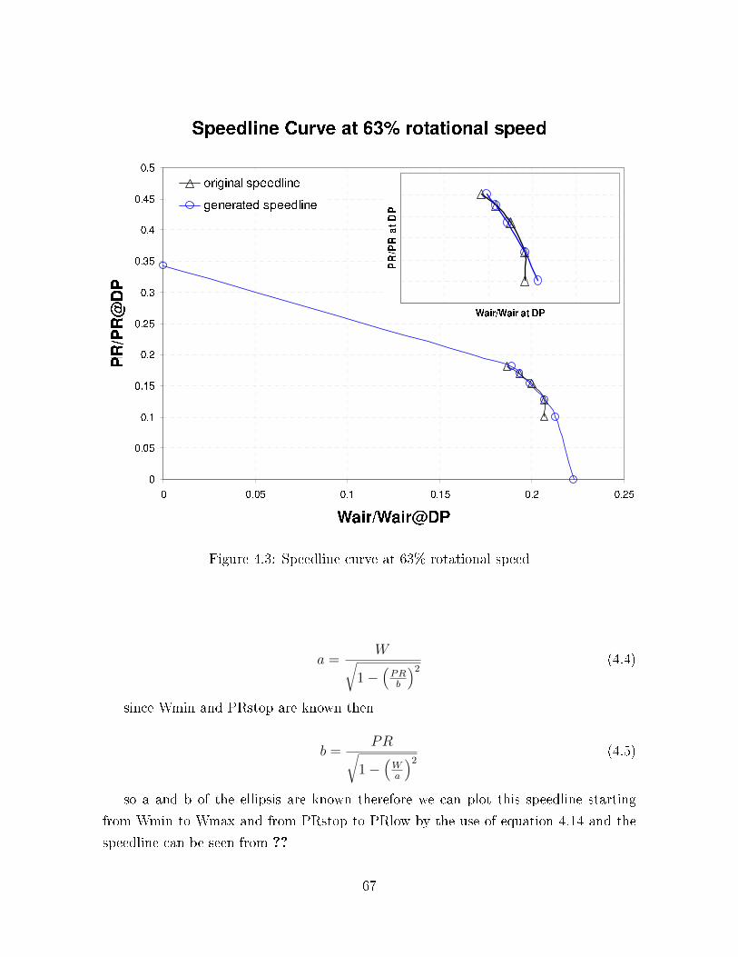
Figure 4.3: Speedline curve at 63% rotational speed

a =W√

1−(PRb

)2 (4.4)

since Wmin and PRstop are known then

b =PR√

1−(Wa

)2 (4.5)

so a and b of the ellipsis are known therefore we can plot this speedline starting

from Wmin to Wmax and from PRstop to PRlow by the use of equation 4.14 and the

speedline can be seen from ??

67

This process is performed for every speedline and the result can be seen in the

following �gure

Figure 4.4: Speedline compressor performance map

Control Analysis

The objective of this analysis is to see which are the parameters that control the shape

and the size of each speedline. Its important at this point to emphasize the fact that

each speedline has the following variables a,b,Wmin and PRstop . Those parameters

are the ones that are going to be analysed in order to initialise optimization's procedure.

Each of these parameter should be expressed as a function of speed since speed is

the most reliable measurement from a family of measurements of a gas turbine

a, b,Wmin, PRstop = f(N)

taking each parameter individually it is concluded that each constant can be ex-

pressed by an equations as seen here

68

The coe�cient a of the ellipsis is an exponential function of speed and coe�cients

a1,a2

a = a1 ∗Na2 (4.6)

The coe�cient b of the ellipsis is an exponential function of speed and coe�cients

b1,b2 and PRdp, where PRdp is the design point pressure ratio.

b = PRdp ∗ (b1 ∗N b2) (4.7)

The coe�cient PRstop determines where each speedline should stop to be plotted

and this can be seen from the following �gure. Generally the boundaries of a compressor

map can be expressed by a simple linear equation where PRstop is a function of a and

PRdp as expressed here

PRstop = ((PRdp ∗ 1.2)− 1) ∗ a+ 1 (4.8)

The mass �ow rate corresponding to the point where the compressor map stops to

be plotted ie.PRstop can be expressed based on the ellipsis equation.

amin =√a2 ∗ (1− (PRstop/b)2) (4.9)

Each speedline will consist of �ve points since PYTHIA's default compressor maps

have �ve points per speedline curve therefore astep is expressed in terms of coe�cients

amin and a.

astep = (amin − a)/4 (4.10)

Now mass �ow can be determined by the following equation as a function of amin

and astep

W = amin + j ∗ astep (4.11)

Since mass �ow W is calculated for each speedline then Pressure Ratio PR can be

determined by the elliptic coe�cients a,b and mass �ow rate W.

PR =√b2 ∗ (1− (W/a)2) (4.12)

69

Totally there are 4 coe�cients that enable the process to determine as accurately

as possible the speedlines from 50% up to 115% of compressor shaft speed. These

coe�cients are going to be determined by the genetic algorithm optimiser in order to

match the operating points targeted. A graph showing the 2 parameters of this ellipsis

expressed with respect to the constant speed is seen from �gures 4.5 and 4.6.

Figure 4.5: Elliptical coe�cient a for LPC, HPC and LM2500 vs shaft speed

70

Figure 4.6: Elliptical coe�cient b for LPC, HPC and LM2500 vs shaft speed

4.2.2 E�ciency

Mathematical Analysis

The e�ciency contours are describing the regions of constant isentropic compressor e�-

ciency. As seen from �gure 4.8 the contours can be described by the cutaway of a three

dimensional ellipsoid shape in the PR-W plane. However there is no analytical solution

for determining the points of intersection between an ellipsoid and an ellipsis therefore

this approach is limited by its complex mathematical nature which in turn makes the

objective of determining the e�ciency wrt compressor shaft speed not feasible. After

an extensive review of mathematical methods for expressing the e�ciency contours an-

alytically as a function of pressure ratio, mass �ow and speed the most straight forward

and generic approach was to extrapolate the intersection points between the speedlines

and the e�ciency contours and plot them against mass �ow rate as seen from �gure

4.7.

71

Figure 4.7: Typical compressor e�ciency map

It can be assumed that each e�ciency line belongs to an elliptic curve with the

following equation

(x− xca

)2

+(y − ycb

)2

= 1 (4.13)

where (xc, yc) are the coordinates of the center of the ellipsis. Assuming the center

at (xc, 0) then equation 4.13is simpli�ed to the following form

(W − xc

a

)2

+(ETA

b

)2

= 1 (4.14)

In order to de�ne this ellipsis accurately it is essential to �nd the parameters a and

b, which determine where the ellipsis is going to meet the x and y axis when ETA=0

and W=0 respectively. The ellipsis that describes the e�ciency lines has the x axis

center at the middle of the speedline's mass �ow rate range and the y axis center at

y=0 as seen from the next �gure. As the mass �ow rate range, for which e�ciency has

to be determined, is known from the speedline generation procedure the only unknown

parameter that has to be de�ned is the the coe�cient b of the e�ciency.

72

Figure 4.8: E�ciency curve at 63% rotational speed

Elliptical coe�cient a is the middle point of the speedline curve and given by the

following equation where Wmax is the

a = (Winitial −Wfinal) (4.15)

Since a and xc are known then the isentropic e�ciency ETA can be determined by

the following equation

b =ETA√

1−(Wa

)2 (4.16)

Control Analysis

The objective of this analysis is to see which are the parameters that control the shape

and the size of each e�ciency line. Each e�ciency line is dependent upon the elliptical

coe�cients a and b . Those parameters are the ones that are going to be analysed in

order to initialise optimisation procedure.

73

Each of these parameter should be expressed as a function of speed since speed is

the most reliable measurement from a family of measurements of a gas turbine

a, b = f(N)

taking each parameter individually it is concluded that each constant can be ex-

pressed by an equations as seen here

The coe�cient a of the ellipsis is determined by the 4.15

The coe�cient b of the ellipsis is a polynomial function of speed and coe�cients

ETAb1,ETAb2 and ETAb3

b = ETAb1 ∗ (N2) + ETAb2 ∗ (N1) + ETAb3 (4.17)

Each e�ciency line will consist of �ve points since PYTHIA's default compressor

maps have �ve points per e�ciency curve therefore astep is expressed in terms of coef-

�cients amin and a.

astep = (amin − a)/4 (4.18)

Since mass �ow W is determined from the earlier speedline procedure then com-

pressor isentropic e�ciency ETA can be calculated by the following equation.

ETA = b ∗√

1−(W

a

)2

(4.19)

There are three coe�cients that enable the process to determine as accurately as

possible the compressor e�ciency from 50% up to 115% of compressor shaft speed.

These coe�cients are going to be determined by the genetic algorithm optimiser in order

to match the operating points targeted. A graph showing the e�ciency distribution

against the compressor shaft speed N is seen from the next �gure.

74

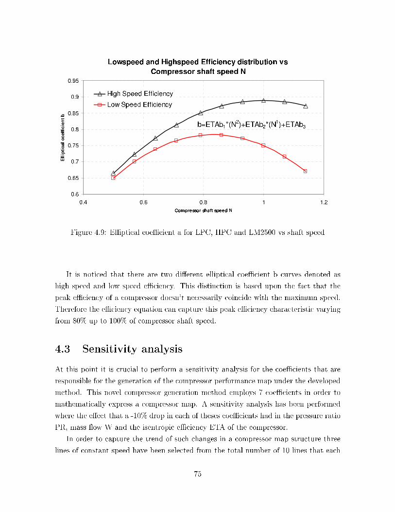
Figure 4.9: Elliptical coe�cient a for LPC, HPC and LM2500 vs shaft speed

It is noticed that there are two di�erent elliptical coe�cient b curves denoted as

high speed and low speed e�ciency. This distinction is based upon the fact that the

peak e�ciency of a compressor doesn't necessarily coincide with the maximum speed.

Therefore the e�ciency equation can capture this peak e�ciency characteristic varying

from 80% up to 100% of compressor shaft speed.

4.3 Sensitivity analysis

At this point it is crucial to perform a sensitivity analysis for the coe�cients that are

responsible for the generation of the compressor performance map under the developed

method. This novel compressor generation method employs 7 coe�cients in order to

mathematically express a compressor map. A sensitivity analysis has been performed

where the e�ect that a -10% drop in each of theses coe�cients had in the pressure ratio

PR, mass �ow W and the isentropic e�ciency ETA of the compressor.

In order to capture the trend of such changes in a compressor map structure three

lines of constant speed have been selected from the total number of 10 lines that each

75

map has. The �rst line at the lowest speed where its parameters like PR,W and ETA

are denoted with number 1, the second line being located at the middle of the compres-

sor map noted as 2 and the �nal line at the maximum speed as 3. Thus by selecting

this representative sample of the compressor map, the e�ect that each coe�cient modi-

�cation implies to the engine performance parameters as PR,W and E�ciency for these

lines is shown in �gure 4.10

Figure 4.10: Sensitivity Analysis of Compressor Map Coe�cients

It is noticed that for the �rst line of constant speed of the compressor map the

coe�cient that has the highest e�ect is the coe�cient W2 followed by W1. These two

factors are included in the equation 5.7

a = a1 ∗Na2 (4.20)

which after the appropriate substitution is

W = W1 ∗NW2 (4.21)

76

The power coe�cient of this equation W2 a�ects the low speed region of the com-

pressor map, which starts from 0.5, more than the high speed region of the map, where

constant speed is nearly 1 and the NW2 part of the equation is close to unity. The

coe�cients W1 and W2 of equation 4.21 are only a�ecting the pressure ratio and the

mass �ow of the compressor map as the value of isentropic e�ciency is determined by

the coe�cients ETAb1,ETAb2 and ETAb3 which are independent of W1 and W2. For

a -10% drop of W1 the pressure ratio and mass �ow rate decrease by -7.5% and -10%

respectively. On the other hand by a -10% drop in W2 the pressure ratio and mass

�ow rate increase by 16% and 20% respectively and the reason for this increase is that

the value of constant speed is less than 1. For the line of the compressor map which

is at a constant speed value higher than 1, the same drop would produce a decrease of

pressure ratio and mass �ow rate PR3 and W3 respectively.

The isentropic e�ciency of the compressor map's low speed region more sensitive

to the coe�cient ETAb2. As the e�ciency lines are expressed as an elliptical equation

the b constant of the ellipsis, which lies in the y axis, is determined by the quadratic

equation 5.6

b = ETAb1 ∗ (N2) + ETAb2 ∗ (N1) + ETAb3 (4.22)

It is concluded that the e�ect of changing the ETAb2 while keeping everything else

the same shifts the curve along the x-axis, and moves it up and down. Speci�cally a

-10% drop in ETAb2 results in a -14% decrease in isentropic e�ciency.

For the second region of the compressor mapW1 andW2 are the coe�cients a�ecting

the pressure and mass �ow rate and ETAb1 and ETAb2 the e�ciency of the compressor.

A -10% drop in W1 decreases PR2 and W2 by -8% and -10% respectively. The e�ect

of W2 drop in this region is smaller that the �rst region for the compressor map as the

value of constant speed in close to unity and its e�ect is a small increase of 2% for both

the pressure ratio PR2 and mass �ow W2. The e�ciency drops by 20% and 10% when

decreasing the coe�cients ETAb2 and ETAb1 respectively.

At the �nal region of high speed of the compressor map the decrease of W1 by -10%

results in a -10% drop in pressure ratio PR3 and mass �ow rate W3. Coe�cient W2

has a smaller e�ect in PR3 and W3 than W1 which is translated in -4% drop for both

PR3 and W3. Finally the e�ciency of this compressor map's region is decreased by

-14% and -26% when dropping by -10% the coe�cients W1 and W2 respectively.

Summarising the most sensitive coe�cients are enlisted here

77

1. For the low speed region

� W2 for PR1 and W1

� ETAb2 for ETA1

2. For the middle speed region


� ETAb1 and ETAb2 for ETA2

3. For the high speed region


� ETAb1 and ETAb2 for ETA3

The e�ect that these coe�cients have in the shape of the compressor map can be seen

analytically from the following �gures. The initial compressor map and the one where

each coe�cient has been decreased, by the same amount as in the sensitivity analysis,

are seen in the same graph in order to extract general trends and patterns that the

map's shape follows for each coe�cient.

Starting by the e�ect that a -10% drop in W1 has in the compressor map it can be

seen from �gure 4.11, where the modi�ed map is in dotted lines, that the compressor

map in the PR vs W plane shifts to the left.

Figure 4.11: E�ect of W1 coe�cient to the compressor map

This is a result of the decrease in mass �ow rate W1 and PR1 that this drop in W1

implies. On the e�ciency map the value of the isentropic e�ciency remains the same,

78

as there is no change in the y-axis coordinates, however the pressure ratio decreases

which in turn displaces the curves along the x axis to the left.

The drop of -10% in W2 a�ects the compressor map as seen in �gure 4.12, where

the map in the PR vs W plane is �shrinked� and compressed in lower boundaries than

the initial map.

Figure 4.12: E�ect of W2 coe�cient to the compressor map

This is due to decrease in mass �ow rate W3 and pressure ratio PR3 for the high

speed region and increase in the low speed region of PR1 and W1. On the e�ciency

map the same e�ect is noticed, again with the isentropic e�ciency values remaining

uninterrupted.

Although the change in PR1 had a very small e�ect in the sensitivity analysis that

has been earlier performed it is important to emphasize that this coe�cient is crucial

for the transition of the compressor map shape from high pressure to low pressure and

vice versa. The maps of high pressure compressors have almost vertical lines at the

high and middle speed regions where for the low pressure the curvature of the lines is

signi�cantly higher. The margin for the PR1 coe�cient is is quite wide for compressor

generation purposes so that a gas turbine user can customise the compressor map, but

for optimisation purposes this margin will be narrowed based on the nature of the

compressor under investigation ie. low, intermediate and high pressure. For this case

where a high speed compressor is represented and in order to have a Representative

modi�ed compressor map the coe�cients PR1 has been decreased by 70% and the e�ect

of this change is seen in �gure 4.13.

79

Figure 4.13: E�ect of PR1 coe�cient to the compressor map

As seen from the �gure above the lines of constant speed in the PR vs W plane

compressor map are not vertical as the initial map but present a curvature that charac-

terises the low and intermediate pressure compressors. If the gas turbine user wishes to

construct a compressor map that will satisfy a low pressure compressor criteria he has

to decrease signi�cantly the value of PR1 for a realistic representation of the compressor

map.

The e�ect that a -10% drop in ETAb1 and ETAb2 have in the compressor map is

seen in �gure4.14. The drop in ETAb1 decreases in turn the isentropic e�ciency as

noticed from the shift of the compressor map along the y-axis . The high speed lines

present a higher decrease that the middle and low speed lines as described earlier in

this section. The pressure and mass �ow rate are not a�ected by the change of ETAb1

coe�cient.

Figure 4.14: E�ect of ETAb1 and ETAb2 coe�cients to the compressor map

Finally the e�ect of the drop of -10% in ETAb2 coe�cient has a similar to ETAb1,

80

e�ect to the compressor map. However the percentage of resulted decrease in the isen-

tropic e�ciency of the compressor is higher here which proves the increased sensitivity

of this coe�cient ETAb2 compared to ETAb1.

The analysis performed justi�es the fact that the compressor performance map re-

lies on the coe�cients that can mathematically describe its shape. In addition it is also

a matter of the appropriate selection of the range, in which each coe�cient lies, for

satisfying the design point criteria of the gas turbine and the nature of the compressor.

This analysis is a useful tool that can guide the gas turbine user to construct a com-

pressor performance map through a program that has been developed and integrated

in PYTHIA's simulation and diagnostics software.

4.4 Demonstration

The program has been developed in visual basic that generates a compressor map based

on the discussed method. The compressor map comprises of 10 speedline and e�ciency

curves. The output of this �le is stored in a text �le ready to be read by both PYTHIA

and Turbomatch. The procedure for generating a compressor performance map can be

seen from the next algorithm.

81

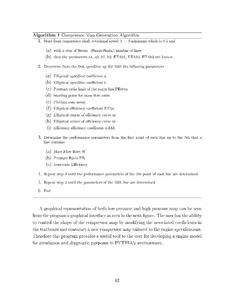
Algorithm 1 Compressor Map Generation Algorithm1. Start from compressor shaft rotational speed N = Nminimum which is 0.5 and

(a) with a step of Nstep=(Nmax-Nmin)/number of lines

(b) then the parameters a1, a2, b1, b2, ETAb1, ETAb2, ETAb3 are known

2. Determine from the �rst speedline up the 10th the following parameters

(a) Elliptical speedline coe�cient a

(b) Elliptical speedline coe�cient b

(c) Pressure ratio limit of the surge line PRstop

(d) Starting point for mass �ow amin

(e) Plotting step astep

(f) Elliptical e�ciency coe�cient ETAa

(g) Elliptical center of e�ciency curve xc

(h) Elliptical center of e�ciency curve yc

(i) E�ciency e�ciency coe�cient ETAb

3. Determine the performance parameters from the �rst point of each line up to the 5th that aline contains

(a) Mass Flow Rate W

(b) Pressure Ratio PR

(c) Isentropic E�ciency

4. Repeat step 3 until the performance paremeters of the 5th point of each line are determined

5. Repeat step 2 until the parameters of the 10th line are determined

6. End

A graphical representation of both low pressure and high pressure map can be seen

from the program's graphical interface as seen in the next �gure. The user has the ability

to control the shape of the compressor map by modifying the associated coe�cients in

the textboxes and construct a new compressor map tailored to the engine speci�cations.

Therefore this program provides a useful tool to the user for developing a engine model

for simulation and diagnostic purposes in PYTHIA's environment.

82

(a) LP Compressor Map PR vs W (b) HP Compressor Map PR vs W

(c) LP Compressor Map ETA vs PR (d) HP Compressor Map ETA vs PR

(e) LP Compressor Map ETA vs W (f) HP Compressor Map ETA vs W

Figure 4.15: Generated Compressor Performance Maps

As seen from �gure 4.15the distribution of speedlines in the PRvs W plane compres-

sor map is exponential which means that as the compressor shaft speed increases the

83

gap between the speedlines increases as well. This e�ect can be mimimised by simply

changing the type of mathematical equation which distributes the coe�cient a of the

ellipsis 4.5. Thus the generated compressor map will be able to capture that e�ect

through a quadratic equation instead of an exponential.

The disadvantage of this process will be the addition of two extra coe�cients that

quadratic equation has to the genetic algorithm optimisation that is employed in the

developed o�-design adaptation. This will result in a further computation time penalty

that can be avoided as the objective is to generate a compressor map that can be

fully controlled mathematically and not to exhaust the accuracy limits by making a

compressor map very case-speci�c. However for future modi�cations of the developed

map generation method this could be explored as the program is modular and enables

further development.

The crucial role that the compressor map has in the adaptation of an engine model to

a service engine at o�-design conditions and the use of genetic algorithms optimisation

technique for achieving the former fundamental objective, follows in the next section.

84

Chapter 5

O�-Design Performance Adaptation

5.1 Introduction

Since e�ective gas turbine performance diagnostics is strongly dependent on accurate

engine performance models near a chosen nominal diagnostic operating condition, such

as design operating condition or full power condition, any noticeable performance pre-

diction errors comparable to performance deviation due to engine degradation may lead

to misleading diagnostic results. To produce an accurate engine model, the following

conditions have to be satis�ed.

� As described in design point adaptation chapter it is of paramount importance

to adapt the engine model to the service engine in order to match the engines

target measurements, by selecting a set of component performance parameters to

be adapted.

� Construction of a compressor map that will meet the engine model speci�cations

and at the same time capture as accurate as possible the compressor map for the

speci�c engine. Although compressor maps are exclusive property of manufactur-

ers and not available to gas turbine users it is well known that all the engines' com-

pressor maps share some common characteristics and patterns with each other,

that have been considered in the compressor generation method. Therefore a con-

struction of an initial map from the design point characteristics of a gas turbine is

quite a straight forward procedure from the compressor generation method that

has been developed. The parameters a�ecting the shape of the performance map

are at the user's disposal to modify for the aforementioned scope.

85

� Adaptation of the engine model to satisfy engine o�-design performance by creat-

ing new engine component maps, as these maps play important role in o�-design

performance predictions. Through the use of genetic algorithms optimise the

coe�cients that mathematically express a compressor map, as in compressor gen-

eration method, in order to minimise the error between the simulated and target

measurements..

Engine o�-design performance represented by measurable parameters, such as gas path

pressures, temperatures, shaft rotational speeds, fuel �ow rate, thrust, etc., heavily

depend on the characteristics of the compressors [37]. Therefore, the shape of the

compressor characteristic maps plays an important role in determining the values of

engine measurable parameters at engine o�-design operating conditions. Thus, if a set

of selected measurable o�-design performance parameters is imposed as a target, the

compressor characteristic maps can be modi�ed in an �inverse� mode to match the

target. Such an approach is called o�-design performance adaptation.

Most gas turbine analytical models proposed in the literature are simply design

models. Some others, however, are able to predict o�-design behavior by means of

zero-dimensional models [38, 8, 1, 17, 18], one-dimensional or more sophisticated mod-

els of the components [26]. The models are referred to as zero-dimensional if only the

thermodynamic transformations across the component are considered without simulat-

ing the internal �ow �eld.

Various methods have been developed for adapting an engine model to a service

engine at part load conditions [39, 40, 8, 14, 25, 12]. The majority of the methods

are using the deck data to construct a compressor map and then through thermody-

namics performance simulation codes match a series of target measurements at part

load conditions. This process has being improved over the years by the inclusion of

optimisation techniques like neural networks and genetic algorithms [41, 42, 43, 38].

The limitation of these methods is the fact that they are very case speci�c. This is

supported by the fact that compressor performance maps are exclusive property of the

engine manufacturer and not always available for determining the performance of an

engine at o�-design conditions. In addition variable geometry compressor scheduling is

not always known and the e�ect that the variable inlet guide vanes have in the shape of

a compressor map shape can not be predicted accurately at a zero dimensional models.

The developed o�-design adaptation method is a novel method that combines a novel

compressor map generation technique with the optimisation capabilities of a genetic

86

algorithm. It is a generic method which covers all the types of compressors from low

pressure and high pressure and has the capacity to adapt the engine model to a series

of o�-design operating points.

To improve the accuracy of gas turbine performance prediction in the vicinity of

engine design point, the compressor map coe�cients that have been established in the

compressor generation method are employed and an adaptive searching approach for

a best set of the coe�cients using a Genetic Algorithm is described. The proposed

adaptation approach is then applied to a model aero gas turbine engine to test the

e�ectiveness of the approach with several case studies. Analysis of the adaptation

results and discussion of the advantages and disadvantages of the method are provided

accordingly.

The compressor map coe�cients de�ned in compressor map generation method are

the ones that will be optimised for the o�-design adaptation. These factors are tuned

through the adaptation process by the genetic algorithm in order to �t the predicted

o�-design performance to the observed o�-design performance. In order to build the

Objective Function (OF) as determined in equation and perform the o�-design adap-

tation process, a set of observed o�-design performance measurements must be chosen

as a target. This set of measurements will be matched with an iterative optimization

procedure by repeatedly adapting the set of compressor map's coe�cients until the

Objective Function reaches its minimum.

Several case studies have been carried out in order to validate the developed adap-

tation method and test its accuracy and limitations. In addition a comparison has been

made between the newly developed o�-design adaptation method with an earlier adap-

tation approach developed by Lo Gatto and Li[39], in order to emphasize the advantages

and disadvantages of the new adaptation method in terms of accuracy, computation

time and future capabilities.

From a series of service engine data the test cases that have been carried out for

this purpose are presented here.

87

Case No Power Output (MW) Target Data Op. Points Method Used Map No1 30.0-29.0 Simulation 2 New Adaptation 3

2 30.0-29.0 Simulation 2 Older GA Method 4

3 30.0-28.0 Simulation 4 New Adaptation 3

4 30.0-28.0 Simulation 4 Older GA Method 4

5 30.0-28.0 MEA 4 New Adaptation 3

6 30.0-28.0 MEA 4 Older GA Method 4




Table 5.2: O�-Design Adaptation Test Cases

The range of the gas turbine's power output, which is the handle of the engine, starts

from 30 MW up to 28 for the �rst six test cases and reaches a minimum of 17.0 MW

for the last two test cases. The number of operating points that the adaptation process

handles extends from two points up to 4 The last two test cases are have in total 12

operating points but these are not completed in one adaptation process but its a sum

of three di�erent adaptations each one having 4 points. The reason for this arti�cial

technique of extending the range of adaptation is that many gas turbines, which have

variable stator vanes for improving their part load performance, have di�erent shape of

compressor maps from high power setting to lower power setting, as this is the case for

test cases 7 and 8.

The source of target data is through simulation for the �rst group of test cases and

Manx Electricity authority service engine data for the second group.

The compressor map used for Lo Gatto adaptation method is a default compressor

map provided by PYTHIA labeled �4� . The compressor map used for the new developed

adaptation is labeled number �3� as this is a customised compressor map that is created

by the developed compressor generation method and altered by the gas turbine to satisfy

the initial design point conditions of any gas turbine engine. 5.2

Accuracy, computation time and limitations of the adaptation is a�ected by the

number of o�-design operating points that the process has to satisfy. A single point

adaptation process is more accurate and signi�cantly faster than a multiple point pro-

cess. In real case scenarios a gas turbine user would prefer to have a series of o�-design

operating points adapted and therefore have a spherical overview of the gas turbine's

performance for the maximum range of operation envelope, that a software programme

88

like PYTHIA can handle. The multiple point adaptation implies a single compressor

map that would satisfy the total number of operating points. Therefore the test cases

presented here are multiple point test cases in order to exhaust the capabilities and

limitations of the adaptation process.

The �rst group of cases studies refers to the �rst four cases, where the observed

o� design performance at di�erent o�-design conditions are simulated with Cran�eld

performance simulation software PYTHIA, by choosing a default compressor map from

PYTHIA as `real' map. The o� design simulation provides simulated measurements that

have been considered as real for validating the o�-design adaptation. At the o�-design

performance adaptation the compressor map generation technique has been employed

in order to construct a initial map that will by modi�ed by the genetic algorithm

optimiser. The Genetic Algorithm is used to tune the coe�cients of the compressor

map to �t the predicted o�-design performance to the �real� o�-design performance.

The user can modify the range of compressor map's coe�cients when setting up the

o�-design adaptation therefore specify the searching space of the optimiser. A similar

process is involved for employing the older adaptation method developed by Lo Gatto

and Li[39]with the di�erences that the compressor map shape is altered only through

the GA optimisation process, the user can not customise a compressor map before the

adaptation , and the shape of the compressor map isn't fully controlled mathematically

as the new developed method. A detailed comparison between the two method will be

ampli�ed in the discussion section of this chapter.

In the second group of case studies, the observed o� design performance at di�erent

o�-design conditions are data provided by MEA. This set of data are obtained at steady

state conditions, selected from a series of available data at similar ambient conditions

and �nally have been corrected before the adaptation process. At the o�-design per-

formance adaptation the compressor map generation technique has been employed as

previously described in the �rst group of case studies. In addition the same target data

have been used for the adaptation method by Lo Gatto.

The sets of compressor coe�cients that ensure a better match for both case studies

are provided during the iterations. Once the Objective Function reaches its minimum,

the best set of compressor map coe�cients is obtained and can be used to produce more

accurate o�-design performance predictions.

89

5.1.1 Genetic Algorithms

A Genetic Algorithm (GA) that follows the idea of Darwin's natural evolution is one

of the optimization searching techniques that have a wide range of applications[44, 45,

46, 47, 48]. The genetic algorithms (GAs) is an adaptive heuristic search algorithm

based on the evolutionary needs of natural selection and genetics. Genetic algorithms

are model based methods which the use a searching and optimization technique [27].

The GAs have the following three operations

1. Selection: chooses the strings for next generation based on the �survival of the

�ttest� criterion

2. Crossover: allows info exchange between strings by swapping parts of the param-

eter vector in order to get �tter strings

3. Mutation: introduces new or prematurely lost info in the form of random changes

applied to random chosen vector components

A real coded GA is used to ensure accurate representation of individuals, the map's

coe�cients, within a GA population. GA is chosen in the o�-design adaptation process

to obtain the best set of compressor map's coe�cients although it is generally known

to be computationally more expensive than conventional optimization methods.

The quality of each set of coe�cients within the GA population is assessed by

its Objective Function (OF) . Thus, a value of OF approaching 0 indicates a good

set of coe�cients while a high value of OF represents a poor set. Along with the three

conventional GA operators mentioned above, an elitism operation is used in this process

[27]. With this operation, the worse strings in GA population of any generation are

replaced with better strings generated by the three conventional GA operations and

a �tter GA population is produced in the next generation. With this process it is

always ensured that the average �tness of the whole population will improve from one

generation to the next. The numbers of crossovers and mutations in each generation

of the GA search is determined by the probabilities assigned to these operators. The

probability of crossover is set at 35% whereas the probability of mutation is set at

30%. The accuracy of the results and the speed of the search depend on the number

of maximum GA generations used and the size of the population. The higher number

of maximum generations with larger size of population the more bene�cial to a more

accurate solution with the drawback of higher computational costs.

90

5.2 Methodology

The characteristics of a compressor can be represented by 4 characteristic variables:

the corrected mass �ow rate (WAC), the pressure ratio (PR), the isentropic e�ciency

(ETA) and the non-dimensional shaft rotational speed (N) relative to its design-point

value. These 4 variables are linked together in two characteristic maps: the PR-WAC

map and the ETA-PR map such that the operating point of the compressor can be

uniquely determined once any 2 out of the 4 variables are speci�ed. More details of

the compressor characteristic maps can be found in the compressor generation chapter.

In engine o�-design performance adaptation analysis, the dependent measurable per-

formance parameter vector (~P ) is a function of the ambient and operating condition

vector (~u) and the independent component characteristics vector.

~P = f( ~X, ~u) (5.1)

O�-design performance adaptation is directly linked to the modi�cation of the com-

pressor characteristics that is part of ~X . When a set of observed measurable o�-design

performance vector ~PM is imposed as a target of the adaptation, the di�erence be-

tween the predicted measurements (~P ) and the observed measurements ( ~PM ) can be

evaluated by means of an Objective Function (OF) de�ned as follows

OF =l∑

j=1

k∑i=1

ai,j

∣∣∣∣∣Pi,j − PMi,j

PMi,j

∣∣∣∣∣ ∗ 100 (5.2)

where PMi,,jare the values of the observed measurements and Pi,j are the corre-

sponding predicted measurements. ai,j are the weighting factors taking into account

the uncertainty of the individual measurements. The uncertainty analysis of the mea-

surements goes beyond the scope of this study and the weighting factors are set for

simplicity, where the number k is the total number of measurable parameters and l the

number of o�-design operating points of the adaptation process.

Based on Equations 5.1 and 5.2, the Objective Function OF can be expressed as a

function of the ~X and the ~u vectors:

OF = F ( ~X, ~u) (5.3)

Thus, for a given o�-design operating condition, the Objective Function (OF) is

used to assess the accuracy of o� design performance prediction; i.e. small value of the

91

Objective Function indicates accurate o�-design prediction and vice versa. To achieve

a good adapted o�-design engine performance model or obtain a minimum Objective

Function, an optimization technique may be used in the o�-design adaptation process.

The o�-design point adaptation uses the design point scaled compressor maps and

rescales them with compressor map coe�cients to match the required performance

target by keeping the same design point [25]. The compressor map coe�cients are

extracted from these equations:

a = a1 ∗Na2 (5.4)

b = PRdp ∗ (b1 ∗N b2) (5.5)

ETAb = ETAb1 ∗ (N2) + ETAb2 ∗ (N1) + ETAb3 (5.6)

The following seven coe�cients W1,W2, PR1, PR2, ETAb1, ETAb2, ETAb3 deter-

mine the shape of the compressor map and are the ones from which genetic algorithm

selects the best set in ordet to perform the o�-design adaptation.

So the compressor map parameters of the adapted map pressure ratio, mass �ow

rate and e�ciency are:

Wfinal = W1final ∗NW2final (5.7)

PRfinal = PRdp ∗ (PR1final ∗NPR2final) (5.8)

ETAfinal = ETAbfinal ∗√

1−(Wfinal

ETAa

)2

(5.9)

where the coe�cients of the performance map have been selected by the genetic

algorithm. Then the compressor map is scaled by the design point scaling factors in

order to match the design point performance of the engine under investigation. These

scaling factors are listed here

SFN,DP =NDP

NMap

(5.10)

92

SFPR,DP =PRDP

PRMap

(5.11)

SFWAC,DP =WACDP

WACMap

(5.12)

SFETA,DP =ETADP

ETAMap

(5.13)

The compressor map scaling that is performed in this o�-design adaptation process

is shown in �gure 5.1.

Figure 5.1: O�-Design Scaling of Compressor Map

The initial compressor map is in dotted lines and the adapted map in solid lines.

The initial design point remains the same for both the initial map and the adapted

map. The initially predicted o�-design point lies in the default compressor map but

doen't match the target measurements of the adpatation. Therefore by generating

new compressor maps the speedlines are repositioned, through the modi�cations of the

aforementioned map's coe�cients, in order to match the target measuremenets. The

�nal o�-design operating point that satis�es these conditions is located in the adapted

map.

The same process is followed for multiple o�-design adaptation where a single

93

adapted compressor map has to satisfy accurately all the target data that each o�-

design operating point has. As seen in �gure 5.2 the scaling takes into account two

o�-design operating points that their target measurments have to matched. Through

compressor generation and the genetic algorithm optimiser the best set of coe�cients

is determined so as to generate a single compressor performance map for the aforemen-

tioned scope.

Figure 5.2: Multiple Operating Points O�-Design Scaling of Compressor Map

As noticed from �gure 5.2 the distance of the second o�-design operating point

between the inital compressor map and the adapted map is greater than that of the

�rst operating point. This is done intentionally in order to emphasize the fact that as

the adaptation moves further away from the design point of the engine the accuracy of

the prediction also drops.

Although this method incorporates genetic algorithms for adapting the performance

of an engine at o� design conditions, this optimisation procedure has various limita-

tions. The accuracy of this adaptation method depends on the accuracy of the initial

engine model, the quality of the compressor map used and on the distance, in terms of

performance, that the pursued o�-design point has with the nominal operating point.

The optimisation procedure for this adapatation mathod can be seen in �gure 5.3.

94

Figure 5.3: Procedure of O�-Design Adaptation

The objective function is the di�erence between the target measurments imposed by

the service engine o�-design performance and the o�-design performance of the engine

model developed. In order to minimise this objective function the genetic algorithm

optimiser is employed. The genetic algorithm initially generates a, speci�ed by the user,

number of possible solutions by varying the values of the compressor map's coe�cients

over a speci�ed range. It then calls Turbomatch code to get the o�-design performance

results of the initial population of compressor maps. The �tness of each set of coe�cients

is then determined. From a series of possible solutions the ones that present the best

�tness are selected for the next generation that is going to occur though crossover

and mutation. Finally this process of evaluation of each individual solution is repeated

through all the processsess of the GA until the limitsa of population size and generations

have been reached. Then the best set of compressor map coe�cients that through

turbomatch simulation present the lowest objective function, therefore the maximum

�tness is provided to the gas turbine user.

95

5.3 Application

To demonstrate the e�ectiveness of the o�-design performance adaptation, di�erent

cases have been tested by adapting di�erent sets of maps of the developed engine

model's compressor brick. Since an engine model, that simulates accurately the service

engine under investigation, has been developed a set of to be adapted parameters has

been selected in order to match the target measurements of the engine at o�-design

conditions. The list of the selected measurable parameters for the o� design performance

adaptation is given in table5.4. The nominal operating point for this con�guration is

at 30 MW with the power output set as the handle of the engine.

No Symbol Performance Parameter Units

1 P3 Compressor Discharge Pressure atm

2 T3 Compressor Discharge Temperature K

3 P6 High Pressure Turbine Pressure atm

4 T6 High Pressure Turbine Temperature K

5 T8 High speed Power Turbine Temperature K

6 � Fuel Flow kg/s

Table 5.4: Measurable Performance Parameters

Test Cases 1 & 2

In the �rst test case the method has been validated by using as reference the simulations

of turbomatch at o� design conditions from 30 MW down to 29 MW with a step of

0.5 MW, with a default compressor map available from turbomatch labeled compressor

map 4. Then the simulated results have been compared with the ones produced by the

developed o�-design adaptation method, which incorporates compressor generation ie.

a di�erent compressor map denoted map 3. The results of the new developed method

indicate a very close match between the �real� and adapted measurements as seen from

table 5.6.

96

Power No Parameter �Real� Earlier DevelopedOutput (MW) Adaptation Adaptation

30 1 P3 22.1 22.1 22.1

2 T3 753.65 753.65 753.65

3 P6 4.529 4.529 4.529

4 T6 1119.15 1119.15 1119.15

5 T8 789.55 789.55 789.55

6 � 1.752 1.752 1.752

29.5 1 P3 21.860 21.873 21.868

2 T3 750.66 752.463 750.9695

3 P6 4.488 4.4855 4.4885

4 T6 1114.49 1116.44 1114.515

5 T8 787.30 788.871 787.325

6 � 1.7273 1.72865 1.727301

29 1 P3 21.62 21.655 21.636

2 T3 747.65 749.2665 748.225

3 P6 4.448 4.4465 4.4485

4 T6 1109.77 1110.567 1109.785

5 T8 785.03 785.675 785.075

6 � 1.7025 1.70275 1.70254

Table 5.6: Test Cases 1 & 2: O�-Design Adaptation Results for �Real� data withDeveloped Adaptation Method and Earlier Adaptation by Lo Gatto

In the second test case again the simulations results from turbomatch o�-design

simulation, for the same power range and with compressor map 4, have been used as

targets for the earlier adaptation method developed by Lo Gatto. In contrary to the

�rst test case the engine model engaged the compressor map 4 in the adaptation process.

The comparison between the two adaptation methods, that have the same targets and

the same engine models, provides a good insight in the e�ect that the compressor map

generation method has in the o�-design adaptation.

The accuracy of the new developed adaptation is higher than the older method as

seen from �gure 5.4 where each targeted measurement is plotted against the power

output of the engine for the whole range of simulation.

97

(a) P3 (b) T3

(c) P6 (d) T6

(e) T8 (f) Ff

Figure 5.4: Prediction of Test Case 1 and 2 Measurable parameters after adaptation vs�Real� data

As seen from the �gure above the adaptation process by Lo Gatto presents a sig-

ni�cant �uctuation, especially at the temperature measurements, at the �rst o�-design

98

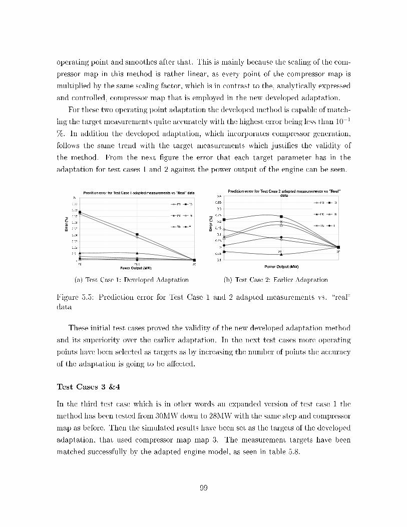
operating point and smoothes after that. This is mainly because the scaling of the com-

pressor map in this method is rather linear, as every point of the compressor map is

multiplied by the same scaling factor, which is in contrast to the, analytically expressed

and controlled, compressor map that is employed in the new developed adaptation.

For these two operating point adaptation the developed method is capable of match-

ing the target measurements quite accurately with the highest error being less than 10−1

%. In addition the developed adaptation, which incorporates compressor generation,

follows the same trend with the target measurements which justi�es the validity of

the method. From the next �gure the error that each target parameter has in the

adaptation for test cases 1 and 2 against the power output of the engine can be seen.

(a) Test Case 1: Developed Adaptation (b) Test Case 2: Earlier Adaptation

Figure 5.5: Prediction error for Test Case 1 and 2 adapted measurements vs. �real�data

These initial test cases proved the validity of the new developed adaptation method

and its superiority over the earlier adaptation. In the next test cases more operating

points have been selected as targets as by increasing the number of points the accuracy

of the adaptation is going to be a�ected.

Test Cases 3 &4

In the third test case which is in other words an expanded version of test case 1 the

method has been tested from 30MW down to 28MW with the same step and compressor

map as before. Then the simulated results have been set as the targets of the developed

adaptation, that used compressor map map 3. The measurement targets have been

matched successfully by the adapted engine model, as seen in table 5.8.

99

Power No Parameter �Real� Earlier DevelopedOutput (MW) Adaptation Adaptation

30 1 P3 22.1 22.1 22.1

2 T3 753.65 753.65 753.65

3 P6 4.529 4.529 4.529

4 T6 1119.15 1119.15 1119.15

5 T8 789.55 789.55 789.55

6 � 1.752 1.752 1.752

29.5 1 P3 21.860 21.886 21.876

2 T3 750.66 754.266 751.279

3 P6 4.488 4.483 4.489

4 T6 1114.49 1118.39 1114.54

5 T8 787.30 790.442 787.35

6 � 1.7273 1.73 1.727302

29 1 P3 21.62 21.68 21.652

2 T3 747.65 750.883 748.8

3 P6 4.448 4.445 4.449

4 T6 1109.77 1111.363 1109.8

5 T8 785.03 786.32 785.12

6 � 1.7025 1.703 1.70258

28.5 1 P3 21.379 21.452 21.4277

2 T3 744.62 747.71 746.466

3 P6 4.407 4.406 4.408

4 T6 1104.97 1105.68 1105.16

5 T8 782.71 783.3 782.87

6 � 1.6777 1.678 1.6778

28.0 1 P3 21.138 21.209 21.202

2 T3 741.55 744.667 744.023

3 P6 4.366 4.3651 4.367

4 T6 1100.1 1100.94 1100.36

5 T8 780.35 781.051 780.56

6 � 1.6528 1.6535 1.653

Table 5.8: Test Cases 3 & 4: O�-Design Adaptation Results for �Real� data withDeveloped Adaptation Method and Earlier adaptation by Lo Gatto

The fourth test case again is similar to test case 2 with the only di�erence being

100

the addition of two extra operating points and everything else being kept the same as

before. This earlier adaptation process presents is tabulated in the table 5.8 and the

comparison remarks remain the same for this test case as well.

The measurements are plotted against power as before and it can be noticed from

�gure 5.6 that the developed adaptation follows a the similar linear trend with the o�-

design simulated measurements. As the power drops, ie moving further away from the

design point of the engine model the adaptation error increases. The earlier adaptation

method although it presents the same �uctuation in temperatures it eases out in the

�nal operating points.

101

(a) P3 (b) T3

(c) P6 (d) T6

(e) T8 (f) Ff

Figure 5.6: Prediction of Test Case 3 and 4 Measurable parameters after adaptation vs�Real� data

Taking into consideration the linear compressor map scaling of the earlier method it

isn't capable of satisfying accurately all the operating points targeted. This behavior is

102

also due to the fact that the method has prioritised the matching of the last operating

point of a multi point adaptation rather than an average distribution of qualitative

adaptation.

For these four point test cases the developed method has a maximum adaptation

error almost 5 times bigger than the test case 1, but it is still in the region of less than

1% as seen in �gure 5.7.


Figure 5.7: Prediction error for Test Case 3 and 4 adapted measurements vs. �real�data

It is also noticed that the pressure and the temperature at the exit of the compressor

present the highest error compared to the other measurements and this is due to the fact

that lines of high rotational speed of the compressor map are almost vertical. Therefore

the pressure of the compressor exit that will be extracted from the compressor map is

dependent upon the number of points that each line is able to contain.

In the compressor map generation process each speedline has 5 points that are evenly

distributed along the speedline. It is obvious that this a�ects the prediction of the

pressure and temperature parameters of the compressor exit, however it isn't a�ecting

the adaptation process as the accuracy achieved is of high order. Although a higher

number of points per speedline can resolve this issue, it will result in an undesirable

computation time penalty.

The key characteristic of the new developed method, apart from the compressor

generation, is its ability to handle multiple point adaptation successfully. The �rst four

test case have tested and validated the new developed adaptation, and will be further

tested in the following test cases where service engine data available from MEA will be

matched.

103

Test Cases 5 & 6

In the �fth test case, the observed o� design performance at di�erent o�-design condi-

tions are data provided by MEA again from 30 MW down to 28 MW with a step of 0.5

MW. This set of data are obtained at steady state conditions, averaged at each power

setting and corrected to the exact same ambient conditions for adaptation purposes.

At the o�-design performance adaptation the compressor map generation technique

has been employed as previously. The results show that there is a similar trend in the

variation of the target measurements and the error between the actual MEA and the

adaptation results are of the magnitude of 10−2. The results for both set of data are

tabulated in table 5.10. The maximum errors are observed as expected in the lowest

power setting of the engine which is at 28MW.

104

Power No Parameter MEA Earlier DevelopedOutput (MW) Adaptation Adaptation

30 1 P3 22.1 22.1 22.1

2 T3 753.65 753.65 753.65

3 P6 4.529 4.529 4.529

4 T6 1119.15 1119.15 1119.15

5 T8 789.55 789.55 789.55

6 � 1.752 1.752 1.752

29.5 1 P3 21.9 22.01 21.91

2 T3 749.95 756.55 749.88

3 P6 4.49 4.502 4.495

4 T6 1111.15 1119.48 1111.31

5 T8 785.65 791.92 785.33

6 � 1.728 1.737 1.725

29 1 P3 21.71 21.81 21.72

2 T3 746.55 751.27 746.46

3 P6 4.441 4.446 4.45

4 T6 1104.15 1107.94 1104.45

5 T8 781.75 784.59 781.17

6 � 1.704 1.707 1.699

28.5 1 P3 21.51 21.64 21.52

2 T3 744.45 749.54 744.35

3 P6 4.400 4.410 4.416

4 T6 1099.15 1102.82 1099.75

5 T8 780.45 783.14 779.60

6 � 1.680 1.684 1.674

28.0 1 P3 21.317 21.44 21.34

2 T3 742.95 747.93 742.75

3 P6 4.342 4.351 4.3664

4 T6 1095.15 1098.72 1095.91

5 T8 778.65 781.29 777.37

6 � 1.672 1.679 1.665

Table 5.10: Test Cases 5 & 6: O�-Design Adaptation Results for MEA data withDeveloped Adaptation Method and Earlier adaptation by Lo Gatto

The predicted o�-design measurable parameters which are the target measurements

105

of this adaptation process are plotted against the service engine data in �gure 5.8. The

service engine data follow a di�erent trend than the �rst test case where the �real� data

where actually o�-design simulation results. The reason for this variation of target

parameters against the power output setting of the service engine has to do with the

data collection process from the MEA. It is fundamental at this point to explain the

logic under which the power station operates. Since MEA has a 2 gas generators, 2

steam generators and one steam turbine con�guration the operation of the power plant

is driven by the island's demand for electricity and when applicable by the importing

demand that UK mainland has from the island. Therefore MEA operates the power

station by having 2 gas turbines running at part load conditions early in the day and

reaching the nominal load at peak demand hours which are in the afternoon. At the

end of the day one engine is shut down since demand has dropped, which leaves only

the one engine operating at part load conditions before the next day comes and this is

repeated.

It becomes clear that the data collected from the control systems have to undergo

some preprocessing and corrections should be applied as steady state conditions data

for such a wide operation regime and duration are extremely rare. The data used for

this test case have been collected from single day of operation at the same operat-

ing conditions and very similar ambient conditions, in order to minimise uncertainties

through corrections. As long as a good sample of data for each power setting has been

averaged it was then corrected back to the original nominal point ambient conditions

and then a single operating point was assigned to each power setting. The PYTHIA

software has a parameter correction utility at the at the main window. However the

o�-design adaptation has the capacity to include di�erent ambient conditions at each

operating point apart from the handle of the engine model which is compulsory for this

process.

The sixth test case employs the older adaptation method by using a default compres-

sor map of PYTHIA as in test cases 2 and 4. The results indicate the same �uctuations

as discussed before and as seen through �gure 5.8 .

106

(a) P3 (b) T3

(c) P6 (d) T6

(e) T8 (f) Ff

Figure 5.8: Prediction of Test Case 5 and 6 Measurable parameters after adaptation vsMEA data

The error of the new developed adaptation is kept at the same levels as before with

the highest error observed at the compressor exit temperature and pressure as seen in

107

�gure 5.9. The older adaptation method has a maximum error of 1% which in terms

of temperatures is translated in 8 to 9 deg. K. Although 1% error is quite normal,

in terms of performance prediction of a gas turbine which is very sensitive on the gas

path measurements this error is signi�cant which in turn a�ects the accuracy of any

diagnostic analysis.


Figure 5.9: Prediction error for Test Case 5 and 6 adapted measurements vs. MEAdata

Test Cases 7, 8 & 9

In this group of test cases the part load performance of the service engine from 29 MW

to 17 MW has been adapted. During the operation of the gas turbine a performance

test has been carried over. At the shutdown of one gas turbine of MEA, which normally

takes 10 min, this process has been expanded for 3 hours and a useful set of data have

been collected. The gas turbine would reduce the power output in several steps and

would operate at each power setting for at least 15minutes in order for the engine to

stabilise its operation. This process has been repeated for several power levels before

reaching a minimum which in this case is 17MW. The bunch of data collected requires

further preprocessing before being set as targets for the adaptation process.

The adaptation process is not able to handle the whole range of this o�-design

operating points in one go. The reason for this is that the adaptation cannot handle

operating points that are at least 7% higher or lower than the operating point of the gas

turbine at which the engine model has been initially adapted through design point adap-

tation. This happens because the design point adaptation makes the model extremely

accurate and tight in terms of �exibility in order to satisfy all the target measurements.

108

The result of this limits the o�-design adaptation to reach much lower or higher than

design point conditions power levels, speed levels or turbine entry temperature levels

depending on what is the handle of the engine.

Turbomatch, which is the core code of performance simulation of PYTHIA, doesn't

converge at such cases as a single compressor map cannot capture the operation of a

gas turbine for such a range. This is mainly due to the fact that component character-

istics especially the ones of the compressor change signi�cantly for a variable geometry

compressor. Although the assumption that a �xed compressor geometry map allows

for successful performance adaptation close to design point conditions or in other word

close the point at which the engine model has been initially adapted this is not the case

for adaptation of the engine model at operating points far away from this benchmark.

The o�-design simulation has the capacity to run at the lowest power levels as its an

iterative procedure which takes into account the operating conditions of the earlier step

from the one it simulates. For example when simulating the o�-design performance of

an engine from 30 MW to 20 MW the simulation code will start at 30MW which is

the design point and with a, predetermined by the user, step will then run the 29 MW

case if the step is 1MW. Having completed the �rst step it will then start from 29 MW

in order to reach the 28MW setting. This is not the case for the o�-design adaptation

where the starting point will always be the design point and therefore the program is

not capable of handling large gaps in terms of performance.

Therefore in this test case the adaptation of the engine model occurs in three dif-

ferent steps. In order to have as less steps as possible the design point adaptation was

performed at the middle operating point of each power output setting. In other words

in the 29 -25 MW power output range the engine model has been adapted at 26.79 MW

in order to allow for the +/- 7% allowance limit that o�-design adaptation can perform

in one simulation. The same applies to the other two test cases 8 and 9.

The results of test cases 7, 8 and 9 can be seen from tables 5.12, 5.14 and 5.16

respectively.

109

Power No Parameter MEA Developed ErrorOutput (MW) Adaptation (%)

29.15 1 P3 22.31 22.41 0.4122 T3 770.81 770.71 -0.0133 P6 4.491 4.499 0.1684 T6 1116.02 1115.09 -0.0835 T8 800.11 805.90 0.7236 � 1.733 1.755 1.259

28.05 1 P3 21.85 21.91 0.2402 T3 765.01 764.99 -0.0023 P6 4.401 4.405 0.0904 T6 1103.07 1102.61 -0.0435 T8 795.62 798.70 0.3866 � 1.684 1.695 0.679

26.79 1 P3 21.33 21.33 02 T3 758.36 758.36 03 P6 4.297 4.297 04 T6 1088.24 1088.24 05 T8 790.48 790.48 06 � 1.627 1.627 0

26.03 1 P3 21.01 20.96 -0.2652 T3 754.35 754.40 0.0063 P6 4.234 4.23 -0.1174 T6 1079.29 1080.26 0.0895 T8 787.37 786.15 -0.1566 � 1.593 1.587 -0.386

25.08 1 P3 20.61 20.49 -0.6252 T3 749.33 749.37 0.0043 P6 4.156 4.145 -0.2854 T6 1068.11 1070.03 0.1795 T8 783.50 780.62 -0.3676 � 1.550 1.536 -0.890

Table 5.12: Test Cases 7 : O�-Design Adaptation Results for MEA data with DevelopedAdaptation Method

110


23.98 1 P3 20.15 20.36 0.9942 T3 743.53 744.26 0.0973 P6 4.066 4.090 0.5784 T6 1055.16 1054.96 -0.0195 T8 779.01 784.22 0.6686 � 1.500698 1.522 1.419

23.10 1 P3 19.79 19.90 0.5462 T3 738.89 739.30 0.0553 P6 3.994 4.009 0.3724 T6 1044.81 1044.69 -0.0115 T8 775.41 778.19 0.3586 � 1.461 1.472 0.800

22.05 1 P3 19.35 19.35 02 T3 733.35 733.35 03 P6 3.907 3.907 04 T6 1032.45 1032.45 05 T8 771.13 771.13 06 � 1.413 1.413 0

20.05 1 P3 18.51 18.22 -1.6032 T3 722.79 721.96 -0.1153 P6 3.743 3.707 -0.9724 T6 1008.90 1010.93 0.2005 T8 762.97 759.58 -0.4436 � 1.323 1.303 -1.492

Table 5.14: Test Cases 8: O�-Design Adaptation Results for MEA data with DevelopedAdaptation Method

111


19.04 1 P3 18.09 18.18 0.5192 T3 717.46 717.84 0.0523 P6 3.660 3.673 0.3534 T6 997.01 996.91 -0.0105 T8 758.84 761.42 0.3406 � 1.277 1.287 0.760

18.03 1 P3 17.67 0.045 02 T3 712.13 -0.009 03 P6 3.577 0.111 04 T6 985.13 0.014 05 T8 754.72 -0.040 06 � 1.232 -0.173 0

17.01 1 P3 17.24 17.20 -0.2512 T3 706.75 706.79 0.0053 P6 3.493 3.489 -0.1114 T6 973.12 973.94 0.0845 T8 750.56 749.44 -0.1486 � 1.186 1.181 -0.366

Table 5.16: Test Cases 9: O�-Design Adaptation Results for MEA data with DevelopedAdaptation Method

What can be easily noticed from the previous tables is that the error is highest at

the boundaries of each power range since the engine model has been adapted initially at

the middle operating point of each test case. This could be avoided by always adapting

the operating point of each test case at its maximum power output. However this would

reduce the margin of adaptation, therefore this approach would require extra test cases

to be simulated in order to cover the same range of operation. The maximum average

error is noticed in fuel �ow which is 0.89% followed by the one in pressure at the exit

of the compressor which is 0.6 %. The general trend that the adapted measurements

follow in relation to the target parameters can be seen in �gure 5.10.

112

(a) P3 (b) T3

(c) P6 (d) T6

(e) T8 (f) Ff

Figure 5.10: Prediction of Test Case 7, 8 and 9 Measurable parameters after adaptationvs MEA Data

As expected the error of each parameter changes sign before and after the operat-

ing point, that the engine model has been initially adapted through the design point

113

Test Case Operating No of Size of GA Minimum Computation

Points Gens Population Fitness OF Time (s)

1 2 1 20 0.81 0.23 24

2 2 1 20 0.65 0.52 20

3 4 1 10 0.54 0.84 60

4 4 1 10 0.36 1.81 30

5 4 1 20 0.79 0.26 100

6 4 1 20 0.55 0.82 60

7 5 2 20 0.71 0.27 140

8 4 2 20 0.78 0.25 120

9 3 2 20 0.80 0.24 110

Table 5.18: Multiple Point O�-Design Adaptation Simulation Properties

adaptation capability of PYTHIA. These test cases have given rise to the limitations

that the developed adaptation has. The strong features of the developed adaptation

and its limitations are discussed in the next section of the chapter.

5.4 Discussion of Results

A group of key parameters that have to be taken into consideration for all the test cases

is the computation time in relation to the genetic algorithm properties and the number

of operating points adapted.Typically for a single point adaptation with 5 generations

and 50 being the population size the process takes almost a minute. The multiple

point adaptation takes considerably longer to converge with the time being almost 6

minutes for 5 generations each one having a population size of 50. The maximum �tness

achieved for the multiple point adaptation test cases, that have been presented, is in

the range of 70 to 80% with the minimum objective function lying between 0.2 and 0.4.

The table 5.18 summarises the simulation properties for all the test cases.

The developed adaptation takes slightly longer than the older adaptation method to

converge as seen in Test case 1 and 2 respectively. However its accuracy is superior to

the earlier method as seen from the �tness of the genetic algorithm which is 16% more

accurate. The minimum objective function is at also improved in comparison with the

earlier method.

In test cases 3 and 4 the size of population is a limiting factor for the accuracy of the

adaptation and this is justi�ed by the �tness values and minimum objective function,

114

which for the earlier adaptation method is unacceptable as it is greater than 1.0. The

time for the developed adaptation to converge is double that of the older adaptation

method and this occurs due to the compressor generation method that is integrated

into the adaptation process. Although the compressor map generation itself is quite

fast in terms as it is an analytical process it is called multiple times from the genetic

algorithm subroutine which requires extra time, especially the intermediate steps of

reading and writing the text�le of the map, before the program converges .

In test cases 5 and 6 where the population size has been increased so did the accuracy

and the computation time of the adaptation. The �tness of the developed adaptation

reaches a level of 0.79 which is very accurate for a multiple point adaptation and

supported by the minimum objective function which is kept as low as possible with a

value of 0.26. The extra time required for this test case cannot be overweighted by the

earlier adaptation method in test case 6 as it is not accurate enough.

In test cases 7, 8 and 9 the number of generations have been increased and this

increased the computation time which exceeds the 2 minutes for test cases 7 which has 5

points. Even in these multiple point cases the accuracy of the developed method remains

its strong feature. A collection of bar charts which summarises the aforementioned

characteristics of the developed o�-design adaptation method can be seen in �gures

5.11, 5.12 and 5.13.

Figure 5.11: GA Fitness for Adaptation Test Cases

115

Figure 5.12: Minimum Objective Function for Adaptation Test Cases

Figure 5.13: Computation Time for Adaptation Test Cases

The setting window of PYTHIA's o�-design adaptation along with the adaptation

result can be seen from �gure 5.14.

116

(a) Adaptation Setting

(b) Adaptation Result

Figure 5.14: O�-Design adaptation setting and Results window

The user has to set the operating conditions of the gas turbine, in the left pink framed

window, which is the power output for this engine con�guration and then select the

target measurements from the right window as seen in �gure 5.14a. The result window

provides the user with the coe�cients of this adaptation process, which are then used

117

for representing the adapted compressor map, the properties of the genetic algorithm

optimiser along with the simulated measurements results and their corresponding errors

as in �gure 5.14b.

Since the adaptation has converged the programme provides the user with a com-

parison graph of the compressor map before and after the adaptation process, in black

and red colour respectively, in order to aid the user determine the direction at which

the compressor map has been shifted to match the o�-design operating point as seen

in �gure 5.15.

118

(a) Compressor Pressure Map before and after Adaptation

(b) Compressor E�ciency map before and after adaptation

Figure 5.15: Compressor Performance maps before and after adaptation

The range of the o�-design operation that the adaptation process is able to cover is

heavily dependent upon the engine model capabilities that Turbomatch simulation code

allows PYTHIA o�-design adaptation to handle. The o�-design adaptation that has

been developed in visual basic and integrated in PYTHIA software has strong features

as its accuracy and its ability to generate a compressor map that captures the engine

performance for the operating points targeted. The programme is robust, modular that

119

allows for further development of both the map generation code and the adaptation code

and user friendly that enables the user to have a complete overview of the o�-design

adaptation.

However the major limitation of the developed adaptation has to do with the margin

that this process is capable of converging successfully. When constructing an engine

model and adapting it through design point adaptation the result of this process is

very case speci�c engine model that meets the target measurements. The side-e�ects of

this process are re�ected in the o�-design adaptation where the o�-design adaptation

isn't allowed to run at o�-design points far away from the point that has been initially

adapted. This isn't a responsibility of Turbomatch as its simulation code is able to

cover a wide range of o�-design operation. The disadvantage is that all the features of

PYTHIA program, which is built in visual basic, are calling the turbomatch code and

extract, required for each case, information without having the ability to modify the

Turbomatch core code and have full control of it. This has limited the adaptation as

its logic is di�erent than the o�-design simulation. The earlier o�-design adaptation

developed by Lo Gatto justi�ed this di�erence as shown in the prediction error �gures

of the previous section.

The new developed o�-design adaptation method narrows this gap between the

o�-design simulation as the behavior of the developed adaptation resembles the sim-

ulation's one as seen from �gures 5.5, 5.7, 5.9. The reason for this lies solely in the

compressor map generation method which facilitates the o�-design adaptation. This

is accomplished by the analytical nature by which the compressor map is expressed in

�rst place and the wide margin for which a user can modify its shape.

The computation time of adaptation depends on the number of operating points,

generations, and the population size of the genetic algorithms. The developed o�-design

adaptation is taking longer than the older adaptation method as its operation includes

extra subroutines that add to the total time for convergence. However the improved

accuracy is of major importance at this point and advantageous to the new developed

o�-design adaptation method. Another advantage of this method is its unique feature of

the compressor map generation that has the potential for a wide range of applications.

The limitations that the adaptation process has doesn't take full advantage of the novel

map generation method that is integrated in it.

The initial adaptation of the engine model, although it is called design point as it

refers to the line speed of 1.0 in the compressor map, is actually an arti�cial design point

that satis�es the target parameters. In test cases 7,8 and 9 where for a wide range of

120

operation three di�erent adaptations have been performed, three di�erent compressor

maps satisfy the targeted operating points. Each compressor map is signi�cantly di�er-

ent from each other but something that allows future exploration and is rec commended

is the combination of these 3 maps. This will produce a single adapted compressor map

that would allow the adaptation to occur in a single simulation.

Another suggestion for this limitation would be the transfer of features from the

design point adaptation to the the o�-design adaptation developed. In other words the

o�-design adaptation should always refer to the previous operating point in a multi-

point adaptation rather than the initial design point. The engine model developed

has a single compressor brick in the o�-design adaptation. However there are gas

turbine con�gurations that have bleed cooling �ows from the compressor that cannot

be modeled as accurately with a single compressor brick in the engine model. The

capability of o�-design adaptation to accommodate more than one compressor brick

would improve the �exibility of the model. The software code is modular enough

that allows further development. A developer's guide has been prepared for assisting

the aforementioned scope. A user's guide has been also written which will assist the

MEA's personnel and any prospective students that will use the developed features of

the PYTHIA.

121

Chapter 6

Gas Turbine Diagnostics

6.1 Introduction

The degradation that an engine experiences during its lifespan operation is classi�ed into

two categories. The �rst one being called �recoverable� referring to compressor fouling,

inlet clogging etc and the other one �non-recoverable� is associated with the engine's

hot end components and parts. Some of the most common degradation occurring in a

gas turbine are the following:

1. Compressor fouling

2. Blade tip clearance increase due to wearing erosion

3. Labyrinth seal damage

4. Foreign and Domestic Object Damage (FOD,DOD)

5. Hot end component damage

6. Corrosion

The e�ect that each type of degradation has in the performance of the gas turbine

components is oftenly expressed in terms of mass �ow capacity and isentropic e�ciency

as summarised in table 6.2

122

Degradation Fault Represented by RangeCompressor Fouling ↓ Γc 0.0 �(-5.0%)

↓ ηc 0.0 �(-2.5%)

Compressor Erosion ↓ Γc 0.0 �(-5.0%)↓ ηc 0.0 �(-2.5%)

Turbine Fouling ↓ Γt 0.0 �(-5.0%)↓ ηt 0.0 �(-2.5%)

Turbine Erosion ↑ Γt 0.0 �(+5.0%)↓ ηt 0.0 �(-2.5%)

FOD ↓ ηc 0.0 �(-5.0%)↓ ηt 0.0 �(-5.0%)

Table 6.2: Component Degradation Table

The performance degradation attributed to the compressor fouling is mainly due to

deposits formed on the compressor blades by particles carried in by the air that are

not large enough (typically a few microns diameter) to be blocked by the inlet �lter

[49]. These deposits result in a reduction of compressor mass �ow rate, compressor

e�ciency and pressure ratio which in turn causes a drop in gas turbine's power output

while increasing its heat rate. This type of degradation is by far the dominant mode.

This degradation can be recovered by regular online and o�-line compressor washing.

Although online washing is not as e�ective as the o�-line washing it is quite common

for peak load con�gurations or single shaft power plants where operation cannot be

interrupted. In combined cycle power plants that have more than one gas turbine

and therefore the �exibility to shut down a gas turbine like MEA and leave only one

engine operating at the end of the day, o�-line washing is preferred. The net �nancial

impact however, is almost always negative unless the fuel purchase price is extremely

high and/or power sale price is too low. Some types of degradation of the LM2500+

engine's hot end components are shown in the �gure below.

The performance degradation associated with hot gas path components is in�uenced

by myriad factors such as fuel quantity, number of starts, amount of water/steam

injection etc. Typically for a base load machine this type of degradation can be 0.2-0.3

percent of the nominal (when new and clean) rating after a months operation[14]. The

123

only remedy for non recoverable degradation is an engine overhaul. The degradation

that hot end components like the nozzle guide vanes, of one GE LM2500+ gas turbine,

have experienced in the MEA's power station after 25,000hrs before the engine was

overhauled can be seen in �gure 6.1.

(a) 1st stage NGV Erosion (b) 2nd stage NGV Erosion

Figure 6.1: LM2500+ Nozzle Guide Vane degradation after 25,000hrs

The diagnostic process is modular and begins with gas turbine data, and applies

data validity analysis to convert the data to more usable information. It then extracts

the knowledge of performance and mechanical trends from the information through

thermodynamic analysis. Then it compares the extracted knowledge to several knowl-

edge bases, and completes a diagnosis or prognosis of the gas turbine's health [50].

Finally it alerts the operator to any important �ndings, and constructs a hierarchy of

potential actions to correct any problems if uncovered. Whatever its speci�c contents

and execution may be, any diagnostic system must rely on discernible changes taking

place in observable parameters in order to detect physical faults [51].

6.1.1 Gas Turbine Diagnostic Schemes

Urban [52] triggered the evolution of gas path diagnostics in the form that is widely

known nowadays, as the nonlinearity of the thermodynamic model has been considered.

The objective function established represents the di�erence of the real and predicted

measurements. Various optimization techniques have been developed to deal with the

minimization problem. This objective function has been minimised by conventional

algorithm which stopped at local minimum [27, 53, 54] . Then Zedda and Singh solved

124

this problem by using the sum of absolute values, minimized through genetic algorithms

[55]. Genetic algorithm optimizer by using information from individual point to assess

engine state have been also used [56]. Escher and Singh [7]considered Jacobian matrix

updates where the solver is nonlinear consisting of successive applications of a linear

one. Mathioudakis et al [50] constructed a composite objective function consisting of

sum of squares and absolute values. A statistical approach has been also explored

[38, 57]where the objective function is a combination and quadratic and a modulus

function.

One of the main reasons for the development of many di�erent methods is the fact

that gas path measurements are di�cult and costly to perform and are thus very limited

in number, in contrast to the large number of parameters needed to be known for engine

health assessment [50]. Methods associated with the diagnosis of gas turbine health are

brie�y described in this subsection.

Kalman Filters

One of the most published methods involve the use of Kalman �lters as the primary

vehicle for fault isolation process. Kalman �lter methods were introduced as a fault

isolation and assessment technique for relative engine performance diagnostics in the

late 1970s and early 1980s. The general approach taken for engine fault diagnosis

typically involves the use of a linearized model approximation evaluated at a selected

engine operating point as proposed by Volponi [58, 43]. This provides a matrix relation-

ship between changes in engine component performance (independent parameters) and

the attendant changes in typically measured engine parameters such as spool speeds,

internal temperatures and pressures, fuel �ow, etc. (dependent parameters).

Neural Networks

Neural networks represent a powerful pattern recognition technique and have been

applied for fault detection of complex systems such as aerospace vehicle, nuclear power

plants and chemical process facilities among others [27, 59]. A key advantage of neural

networks over other methods is their ability to recognize relationships between patterns

despite the presence of noise contamination and/or partial information. More than

85% of published applications have used the feed forward back propagation network

(FFBPN) [50]. A three layer feed-forward network has been used by Volponi [58]. The

feedforward network is trained using supervised learning, which involves presenting

125

input output pairs to the ANN and then using the back propagation (BP) algorithm

to learn the relationships between the inputs and outputs. The input data has been

normalized and the data data used for training was not used for testing the neural

network.

The neural network proposed by Depold [59] acts as templates to eliminate bad data

much the same as analysis would with their rules of thumb. These templates identify

spurious input errors . The �rst two ANN templates identify errors that result in all

output parameters being either high out of statistical limits or low out of statistical

limits. The remaining four ANN templates detect single parameter limit exceedences

that are not physically possible. In the former study when �ve key jet engine parameters

(EPR,EGT,Wf,N2, N1) are considered, six basic templates can be de�ned which

corrects approximately 9% of typical data. The neural networks disadvantage is the

time required for their training but since this training is completed the computation is

very fast and they can also deal with measurement noise and bias.

Bayesian Belief Networks

Bayesian belief networks (BBN) have been described by Romessis [60] . BBN repre-

sents the relation among variables of aerothermodynamic nature of an engine, compo-

nent faults can be detected anytime measurements of gas path variables are available.

Measurement noise, bias and changing operating condition a�ect the accuracy of the

BBN since the thermodynamic relations are altered and the operating points shifted .

Lee and Mavris [61] maintained the generality and the accuracy together, by multiple

Bayesian models tailored to various fault situations where the have been implemented

in one hierarchical mode

Gas Path Analysis

Gas path analysis (GPA) is a powerful diagnostic technique that has been extensively

used to predict the health of a gas turbine, by using the variety of measurements lo-

cated in the engine's gas path. This technique enables the gas turbine user to construct

a reliable and robust maintenance strategy. Therefore the highly considerable main-

tenance and operational costs of gas turbines are reduced. Comprehensive reviews of

gas path diagnostics techniques have been provided by Li [50] and Singh [37]. The gas

path analysis initiated as a linear approach introduced by Urban [52] and followed by

Stamatis et al [26] approach which considered the non-linearity e�ects of the problem.

126

However the limitations addressed by the repeatable uncertainties of the gas turbine

system, motivated the development of various conventional and arti�cial optimisation

techniques like neural networks [56], genetic algorithms [56], hybrid systems [60] and

fuzzy expert systems [62]. Since the GPA is a model-based performance diagnostic

technique thence the accuracy of the diagnostic analysis is dependent on extremely ac-

curate performance simulation. The development of techniques to adapt a performance

engine model to the measurements of a particular gas turbine engine is highly pursued.

A design point performance adaptation method has been developed by Li [21]. The

gas turbine's o�-design performance adaptation is a more complex method which in-

corporates the development and the mathematical scaling of engine component maps as

described in the previous chapter. Accuracy of such a prediction is highly dependent on

the quantity of available engine design data and the quality of component characteristic

maps. Many researchers have explored this topic for its catalytic role in the diagnosis

since it increases the accuracy of engine performance model.

There are so many repeatable uncertainties involved during the operating life of

a gas turbine like changes in ambient and operating conditions, noisy measurements

and faulty instrumentation, all of which contribute to the added complexity of the di-

agnosis. Many performance software, that can handle a series of the aforementioned

uncertainties, have been developed for academic and commercial use based on a fam-

ily of diagnostic techniques [12]. The performance simulation and diagnostics software

PYTHIA, that has been developed in Cran�eld University and updated with a series of

capabilities like the developed compressor generation method and the o�-design adap-

tation, is the one used for this study. In this test case a gas path analysis method will

be employed, through the use of PYTHIA software, in order to determine the actual

degradation of an aeroderivative gas turbine. This application procedure commences

with the development of an engine performance model, continues with the performance

adaptation for matching the real engine measurements, pre-processes ambient and op-

erating condition correction and concludes with the prediction of the engine component

degradation using the concept of GPA index.

6.2 Gas Path Analysis Methodology

The basis of engine health monitoring schemes is to measure fundamental parameters

such as speed, pressure, temperature, fuel �ow and vibration levels and from these

127

measurements deduce the health of the plant by observing changes in the relationships

between them [50]. Some monitoring may be carried out by observation of directly

measured parameters but a deeper insight can be obtained by the use of gas path

analysis which can determine critical performance parameter, such as air�ow, turbine

inlet temperature, and component e�ciencies.

The estimation of health parameters is considered successful when the quantities

measured on the engine are reproduced in the best possible way by, an engine perfor-

mance model incorporating the health parameter [37]. To make the GPA successful the

following criteria must be satis�ed:

1. Performance adaptation improves the accuracy of the simulation

2. Selection of instrumentation set for better visibility analysis of engine health

3. Measurements data preprocessing to reduce the in�uence of measurement noise

and deviated ambient and operating conditions

4. Sensor failure detection and engine component fault diagnosis

A linear and non-linear GPA approach developed at Cran�eld [37] is an e�ective tool

for inverse mathematical problems such a gas turbine performance adaptation and

performance diagnostics. The idea of the method, which is similar as the design point

adaptation process, is as follows. The thermodynamic relationship among performance

parameters, component parameters and ambient, operating condition parameters can

be represented with equation 6.1.

~z = h(~x, ~y) (6.1)

where ~z ∈ <M is the measurable performance parameter vector and M is the number

of performance parameters, and ~x ∈ <N is the health parameter vector and N is the

number of component parameters and h( ) is a vector valued function.

At an initially given design point which is denoted with subscript �0� equation x

can be expanded in a Taylor series as:

~z = z0 +∂h(~x, ~y)

∂x

∣∣∣∣∣0

· (~x− ~x0) +∂h(~x, ~y)

∂y

∣∣∣∣∣0

· (~y − ~y0) +HOT (6.2)

128

HOT represent higher order terms which can be neglected. represents higher order

terms of the expansion and can be neglected. Therefore, a linearised relationship gas

turbine performance model can be expressed with equation 6.3.

∆~z = H ·∆~x+H′ ·∆~y (6.3)

When there is no deviation from standard ambient condition and nominal operating

condition, ∆~y = 0 . So

∆~z = H ·∆~x (6.4)

For any expected deviation of ∆~z from its initial point, the deviation of to-be-

adapted component parameters from its initial point can be predicted by inverting the

in�uence coe�cient matrix (ICM) H to a fault coe�cient matrix (FCM) H−1 leading

to the following equation when N = M

∆~x = H−1 ·∆~z (6.5)

The non-linearity of the engine behavior is taken into account by using an iterative

Newton-Raphson process where linear GPA is applied iteratively until a converged

solution is obtained. The number of component parameters, M , may not be equal.

If N > M Equation (4) is under-determined. Typically such a situation leads to an

in�nite number of least-squares solutions. A pseudo inverse is de�ned as

H# = HT · (HHT )−1 (6.6)

The solution resulting from this, which is the best in a least square sense, is:

~x = H# · ~z (6.7)

If N < M equation x is over-determined and there are redundant equations. A


H# = (HTH)−1 ·H−T (6.8)

129

The resulting solution, which is also the best in a least square sense, is:

~x = H# · ~z (6.9)

The convergence of this iterative adaptation calculation process is declared when

the performance is very close to the measured performance. The root mean square

(RMS) of the di�erence between predicted and real performance is smaller than σwhen

convergence criterion is satis�ed.

RMS =

√∑(zi,predicted − zi,measured)2

M< σ (6.10)

where σ is a very small number (σ=0.001 is usually chosen). The prediction error γi for

each measurable performance parameter is described by the relative di�erence between

the predicted and measured engine performance parameter and expressed with equation

6.11

γi =zi,predicted − zi,measured

zi,measured

· 100% (6.11)

(1) Where γi is the prediction error for the performance parameter. This diagnostic

method is simple and fast in prediction although it has certain requirements that must

be met such as

� The in�uence coe�cient matrix (ICM) is an accurate mathematical description

of gas turbine performance around a speci�c operating point.

� Measurement bias and noise free sensors

� Un-correlated (independent) measurements being sensitive to engine degradation.

A disadvantage of the GPA is its dependency on the apriori information of degraded

components. To e�ectively isolate the deteriorated components GPA index is intro-

duced. The GPA index is a measure of the diagnostic accuracy and is de�ned as:

λ =1

1 + ε(6.12)

where λ is the GPA index and εis the di�erence between measured and predicted

deviations of engine gas path measurements expressed with the following.

ε =∑

wi

∣∣∣∣∣∆zi −∆zm,j

z0,i − z0,j

∣∣∣∣∣ · 100% (6.13)

130

where wi are the weighting factors taking into account the relative importance of

the measurements. To apply the GPA index e�ectively to gas turbine component fault

diagnosis, the maximum number of simultaneously degraded engine components and

the component fault cases (CFC) should be assumed. The diagnostic approach that

covers all the pre-assumed engine fault cases is shown in �gure 6.2 where the highest

values of GPA indices indicate the most likely engine degradation test cases.

Figure 6.2: GPA diagnostic process chart

In a situation where more than one CFC cases are likely, weighted degradation is

suggested and calculated as follows

xi =Sf∑j=1

xi,j · λj/Sf∑j=1

λj

√√√√√√n∑

i=1

error2i

n(6.14)

where xi is a weighted health parameter, xi,j the ith health parameter predicted

in CFC case j, λj the GPA index in CFC case jand Sfthe total number of the most

likely faults. Summarising this diagnostic system which is based on GPA has been

implemented into Cran�eld gas turbine performance analysis software PYTHIA [22]

developed from TURBOMATCH, the validity of which has been tested over many

years.

131

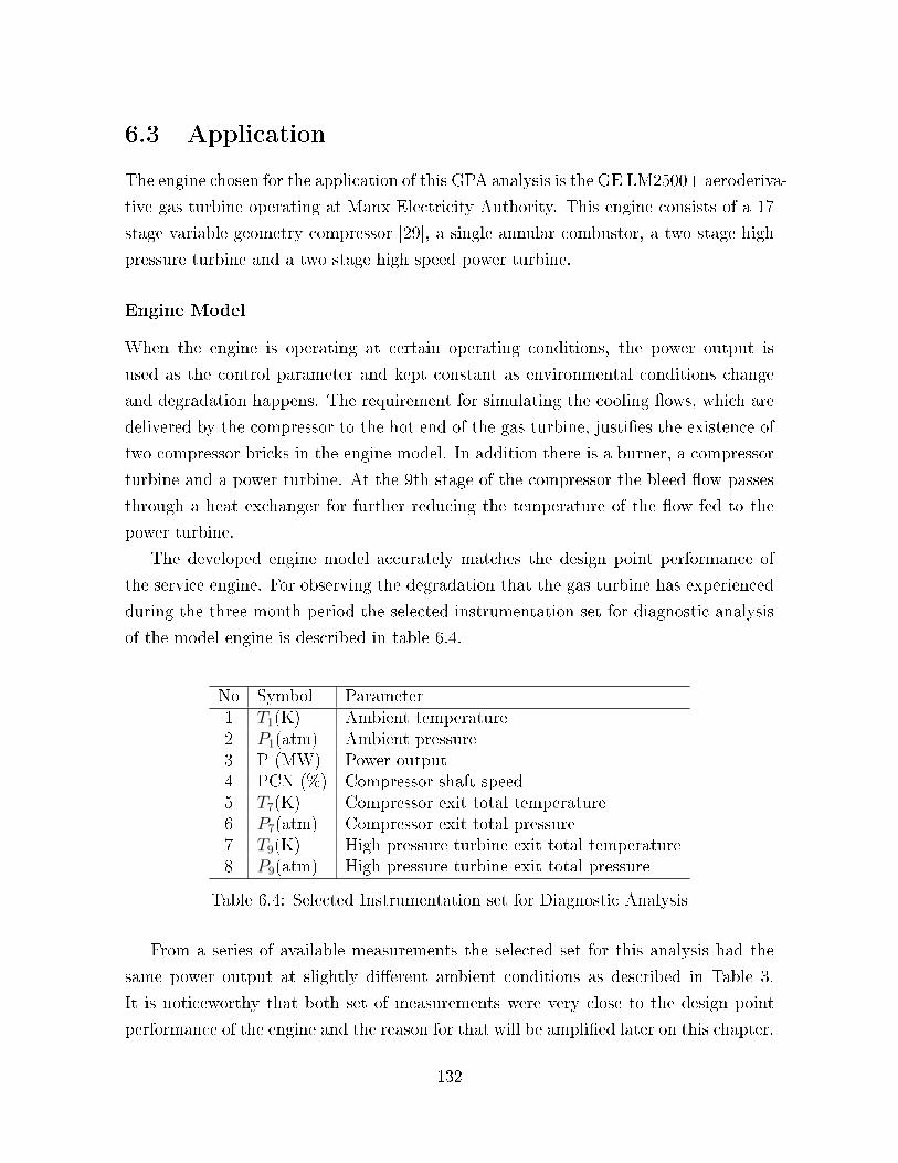
6.3 Application

The engine chosen for the application of this GPA analysis is the GE LM2500+ aeroderiva-

tive gas turbine operating at Manx Electricity Authority. This engine consists of a 17

stage variable geometry compressor [29], a single annular combustor, a two stage high

pressure turbine and a two stage high speed power turbine.

Engine Model

When the engine is operating at certain operating conditions, the power output is

used as the control parameter and kept constant as environmental conditions change

and degradation happens. The requirement for simulating the cooling �ows, which are

delivered by the compressor to the hot end of the gas turbine, justi�es the existence of

two compressor bricks in the engine model. In addition there is a burner, a compressor

turbine and a power turbine. At the 9th stage of the compressor the bleed �ow passes

through a heat exchanger for further reducing the temperature of the �ow fed to the

power turbine.

The developed engine model accurately matches the design point performance of

the service engine. For observing the degradation that the gas turbine has experienced

during the three month period the selected instrumentation set for diagnostic analysis

of the model engine is described in table 6.4.

No Symbol Parameter1 T1(K) Ambient temperature2 P1(atm) Ambient pressure3 P (MW) Power output4 PCN (%) Compressor shaft speed5 T7(K) Compressor exit total temperature6 P7(atm) Compressor exit total pressure7 T9(K) High pressure turbine exit total temperature8 P9(atm) High pressure turbine exit total pressure

Table 6.4: Selected Instrumentation set for Diagnostic Analysis

From a series of available measurements the selected set for this analysis had the

same power output at slightly di�erent ambient conditions as described in Table 3.

It is noticeworthy that both set of measurements were very close to the design point

performance of the engine and the reason for that will be ampli�ed later on this chapter.

132

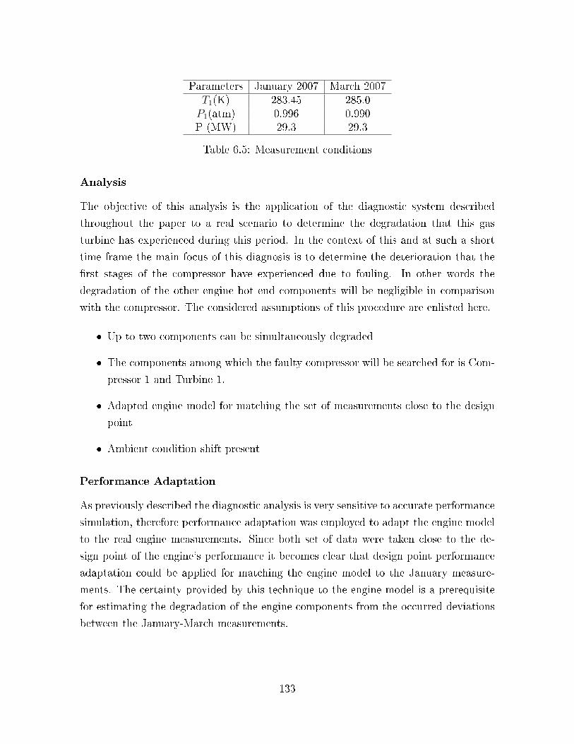
Parameters January 2007 March 2007T1(K) 283.45 285.0P1(atm) 0.996 0.990P (MW) 29.3 29.3

Table 6.5: Measurement conditions

Analysis

The objective of this analysis is the application of the diagnostic system described

throughout the paper to a real scenario to determine the degradation that this gas

turbine has experienced during this period. In the context of this and at such a short

time frame the main focus of this diagnosis is to determine the deterioration that the

�rst stages of the compressor have experienced due to fouling. In other words the

degradation of the other engine hot end components will be negligible in comparison

with the compressor. The considered assumptions of this procedure are enlisted here.

� Up to two components can be simultaneously degraded

� The components among which the faulty compressor will be searched for is Com-

pressor 1 and Turbine 1.

� Adapted engine model for matching the set of measurements close to the design

point

� Ambient condition shift present

Performance Adaptation

As previously described the diagnostic analysis is very sensitive to accurate performance

simulation, therefore performance adaptation was employed to adapt the engine model

to the real engine measurements. Since both set of data were taken close to the de-

sign point of the engine's performance it becomes clear that design point performance

adaptation could be applied for matching the engine model to the January measure-

ments. The certainty provided by this technique to the engine model is a prerequisite

for estimating the degradation of the engine components from the occurred deviations

between the January-March measurements.

133

Initial Correction of Measurements

All the available measurements of March were corrected to the same ambient condi-

tions of the earlier January measurements. As the operating conditions were at the

same power output the apparent deviation was due to degradation and mainly due to

compressor fouling as the engine hasn't experienced any sort of maintenance action

during that period. A comparison between the deviation of the engine performance

parameters with and without correction is presented in �gure 6.3.

Figure 6.3: Engine parameter deviation with and without corrections

Engine Component Fault Detection

To identify which engine component is responsible for the observed deviation the GPA

Index is used. Assuming that the maximum number of simultaneously degraded com-

ponents can be up to two the component fault cases are listed in table 6.6.

Component Fault Case Pre-de�ned faulty components1 Compressor 12 Turbine 13 Compressor 1 + Turbine 1

Table 6.6: Fault Cases

134

The Component Fault Cases with their corresponding GPA index is represented in

�gure 6.4.

Figure 6.4: Componenet Fault Cases GPA Index

It is evident from Figure 5 that CFC 1 and CFC3 present the highest GPA index

therefore there is a deterioration of the compressor and a very small deterioration of the

compressor turbine. In order to determine the actual degradation of each component

and since two of the CFC are likely responsible for the apparent parameter deviation,

the weighted solution is applied. This provides the diagnostic results tabulated in table

6.7.

Component e�ciency Mass �ow capacityEngine Component ∆η (%) ∆Γ (%)

Compressor 1 -0.79 -0.67Turbine 1 -0.09 0.02

Table 6.7: Componenet Degradation Results

As expected the �rst stages of the compressor had a drop of 0.79% in isentropic e�-

ciency and a 0.67% reduction in mass �ow capacity. The degradation of the compressor

turbine is negligible compared to that of the compressor's. The compressor fouling has

an immediate e�ect on the performance of the gas turbine which results in lost power.

The engine's control reaction to the above degradation was to add more fuel and run

135

at slightly higher rotational speed to satisfy the power output, which is the control

parameter of this gas turbine con�guration.

Gas path analysis is a powerful diagnostic technique and its dependencies on accu-

rate performance simulation and a-priori information about degraded components are

compensated by performance adaptation and GPA index respectively. GPA's advantage

is that has a fast solution that represents intrinsic relationship between engine perfor-

mance and aerothermodynamic parameters [27]. GPA and derivatives are powerful

but have the disadvantages of requiring a priori info of degraded components, mea-

surement noise and bias free sensors [63]. From the development of an engine model

and its adaptation to real engine measurements, which is considered fundamental for

such kind of analysis, to the consideration of practical issues of measurement correction

and instrumentation selection this GPA method has the capacity to predict component

degradation at a reliable level. The analysis showed that during a continuous operation

of three months and close to the date of the engine's major overhaul the �rst stages of

the compressor have deteriorated due to fouling. The application of this technique to

this real case scenario facilitates gas turbine users with the operation and maintenance

decision making of the power plant.

136

Chapter 7

Conclusions and Future

Recommendations

This thesis has focused in the development of a performance o�-design adaptation

method software programme that can be integrated to a power station's environment

as a virtual gas turbine performance and diagnostics tool. The main results can be

summarised as follows:

1. A new engine model has been developed in PYTHIA for simulating the perfor-

mance of the MEA's gas turbines at both design and o�-design conditions.

2. The crucial part of progressively re�ning the engine model, based on the collated

service engine data, is accomplished through the design point adaptation method

and an application test case has been presented.

3. A novel compressor map generating method has been developed and integrated

in PYTHIA software. The compressor map is generated based on a family of

coe�cients than capture the shape of such a map, therefore enabling the gas

turbine user to modify these coe�cients and determine a performance map that

will meet the design point criteria of a gas turbine.

4. The compressor map generation is extensively being employed by the o�-design

adaptation method developed.

5. An adaptation method for matching the engine model's performance to that of

the service engine of MEA at o�-design conditions has been developed. This

adaptation process regenerates compressor maps with the appropriate coe�cients

137

and then minimises the di�erence between the predicted and actual measurements

through the genetic algorithms optimiser. The accuracy of this developed method

has been validated and tested. The results of the test cases proved that the

developed adaptation is an e�ective and accurate method for single and multiple

operating point prediction of a gas turbine's performance at o�-design conditions.

6. Convergence time of the adaptation method depends on the genetic algorithms

characteristics and the number of o�-design operating points that are to be mod-

eled. For a typical single point adaptation this is a matter of seconds where for

multiple adaptation this takes a couple of minutes.

7. Gas turbine performance based diagnostics by using the Gas Path Analysis have

been used extensively throughout this research for predicting the health of the

gas turbines at MEA. An application test case showed that this GPA method can

be used for a fast and accurate assessment of a gas turbine's health condition.

Performance adaptation and GPA index must be employed in this process for

ensuring the accuracy of the diagnosis.

8. All these software capabilities, that have been developed, are integrated in the

latest version of PYTHIA that will be delivered to MEA. The software programme

will be a virtual gas turbine tool that will have the capacity to load a series

of measurements, taken from the control systems, and perform the appropriate

actions like measurement corrections,noise reductions, performance adaptation

and diagnostics analysis so that trends of the gas turbine's performance over a

wide range of operation will aid the power plant's maintenance strategy.

Interesting future research directions worth considering in the context of performance

adaptation are:

1. Updating the compressor map generation with more set of equations, that can

describe the shape of the compressor map, so that the user can select from a series

of equations types, the corresponding level of accuracy and predicted computation

time, the one that best matches his criteria.

2. The o�-design adaptation currently can employ the compressor map generation

for a single compressor brick in the engine model con�guration. This feature

prompts the further development of the programme so that the adaptation will

138

be able accommodate more that one compressor bricks with their corresponding

compressor performance maps be handled by the generating method.

3. A very key element that a�ects the �exibility of the o�-design adaptation is the

extent by which PYTHIA makes full use of turbomatch code. Currently this

method has the ability to model up to a speci�c range lower and upper the

point, at which the design point adaptation has been performed. Arti�cially the

adaptation can reach the lowest power level and o�-design conditions but this will

be performed by a series of simulations and not by a single simulation. Therefore

the software should employ extra features from turbomatch code, that are only

available at o�-design simulations in order to increase the range by which o�-

design adaptation can be performed.

139

Bibliography

[1] R. K. Agrawal, B. D. MacIsaac, and H. I. H. Saravanamuttoo. Analysis procedure

for the validation of on-site performance measurements of gas turbines. American

Society of Mechanical Engineers (Paper), (78 -GT-152), 1978.

[2] M. Mucino. EngD Thesis:CCGT performance simulation and diagnostis for oper-

ations optimisation and risk management. University of Cran�eld, 2007.

[3] S. C. Gullen, P. R. Gri�n, and S. Paolucci. Real-time on-line performance di-

agnostics of heavy-duty industrial gas turbines. Journal of Engineering for Gas

Turbines and Power, 124(4):910�921, 2002.

[4] L. Vieria, C. Matt, V. Guedes, M. Cruz, and F. Castelloes. Maximization of the

pro�t of a complex combined-cycle cogeneration plant using a professional process

simulator. J. Eng. Gas Turbines Power, Issue 4, paper, Volume 132, 2010.

[5] C. E. Neilson, D. G. Shafer, and E. Carpentieri. Lm2500 gas turbine fuel nozzle

design and combustion test evaluation and emission results with simulated gasi-

�ed wood product fuels. Journal of Engineering for Gas Turbines and Power,

121(4):600�606, 1999.

[6] L. Smith. Axial compressor aerodesign evolution at general electric. Journal of

Turbomachinery, 124, 2002.

[7] P. Escher and R. Singh. An object oriented diagnostics computer program suitable

for industrial gas turbines. International Congress of Combustion Engines, 21st,

Switzerland, 1995.

[8] A. Alexiou and K. Mathioudakis. Development of gas turbine performance models

using a generic simulation tool. Proceedings of the ASME Turbo Expo, 1:185�194,

2005.

140

[9] K. Mathioudakis. Gas turbine test parameters corrections including operation with

water injection. Journal of Engineering for Gas Turbines and Power, 126(2):334�

341, 2004.

[10] A. J. Meacock and A. J. White. The e�ect of water injection on multispool gas

turbine behavior. Journal of Engineering for Gas Turbines and Power, 128(1):97�

102, 2006.

[11] Philip P. Walsh and Paul Fletcher. Gas turbine performance [Book]. Oxford,

United Kingdom/Fair�eld, NJ: Blackwell Science, Ltd./ASME Press, 1998. 130

ref.

[12] NATO Technical Report. Performance prediction and simulation of gas turbine

engine operation for aircraft, marine, vehicular and power generation. Final report

of the RTO applied vehicle technology, 2007.

[13] S. Gulen and R. Smith. A simple mathematical approach to data reconciliation in

a single-shaft combined cycle system. J. Eng. Gas Turbines Power, Issue 2, paper,

131, 2009.

[14] P. Pilidis. Digital simulation of gas turbine performance. PhD Thesis, University

of Glasgow, 1983.

[15] E. Tsoutsanis, Y. G. Li, P. Pilidis, and M. Newby. Gas path analysis applied to

an aeroderivative gas turbine used for power generation. International Confer-

ence on Condition Monitoring and Machine Failure Prevention Technologies, 5th,

Edinburgh, Proceedings, 2008.

[16] E. Tsoutsanis, Y. G. Li, P. Pilidis, and M. Newby. Gpa diagnostics: An application

to an industrial gas tubine. Cran�eld Multi-Strand Conference, 1st, Cran�eld, 2008.

[17] H. I. H. Saravanamuttoo and B. D. MacIsaac. Thermodynamic model for pipeline

gas-turbine diagnostics. Journal of Engineering for Gas Turbines and Power, pages

875�884, 1983.

[18] P. Zhy and H. I. H. Saravanamuttoo. Simulation of an advanced twin-spool indus-

trial gas turbine. Journal of Engineering for Gas Turbines and Power, 1992.

[19] J. Kurzke. How to get component maps of an aircraft gas-turbine's performance

calculations. ASME paper,96-GT-164, 1996.

141

[20] E. Tsoutsanis, Y. G. Li, P. Pilidis, and M. Newby. Industry university collabora-

tion: A case study between the manx electricity authority and cran�eld university.

Annual Board Meeting of the Institution of Diesel and Gas Turbine Engineers,

2009.

[21] Y. G. Li, P. Pilidis, and M. A. Newby. An adaptation approach for gas turbine

design-point performance simulation. Journal of Engineering for Gas Turbines and

Power, 128(4):789�795, 2006.

[22] Y. Li M. Mucino. An advanced gas turbine gas path diagnostic system using

gpa-index. In Proceeding of COMADEM, 2005.

[23] Y. Li. Gas turbine performance and health status estimation using adaptive gas

path analysis. J. Eng. Gas Turbines Power, Issue 4, paper, 132, 2010.

[24] M. Mucino, J. Ojile, Y. G. Li, and M. Newby. Advanced performance modelling of

a single and double pressure once through steam generator. GT2007-27505, ASME

Turbo Expo 2007, Montreal, Canada, 2007.

[25] W. P. J. Visser, O. Kogenhop, and M. Oostveen. A generic approach for gas

turbine adaptive modeling. Journal of Engineering for Gas Turbines and Power,

128(1):13�19, 2006.

[26] A. Stamatis, K. Mathioudakis, and K. Papailiou. Adaptive simulation of gas tur-

bine performance. J. Eng. Gas Turbines Power, Issue 2, paper, 112, 1990.

[27] H. S. Tan. Fourier neural networks and generalized single hidden layer networks

in aircraft engine fault diagnostics. Journal of Engineering for Gas Turbines and

Power, 128(4):773�782, 2006.

[28] E. Tsoutsanis. PhD First Year Review:Performance adaptation and virtual gas

turbines for power generation applications. University of Cran�eld, 2007.

[29] A. R. Wadia, D. P. Wolf, and F. G. Haaser. Aerodynamic design and testing of an

axial �ow compressor with pressure ratio of 23.3:1 for the lm2500+ gas turbine.

Journal of Turbomachinery, 124(3):331�340, 2002.

[30] J. Klapproth, M. Miller, and D. Parker. Aerodynamic development and perfor-

mance of the cf6-6/lm2500 compressor. International Symposium on Air Breathing

Engines, 4th, Orlando, pages 243�249, 1979.

142

[31] C. Kong, J. Ki, and M. Kang. A new scaling method for component maps of gas

turbine using system identi�cation. Journal of Engineering for Gas Turbines and

Power, 125(4):979�985, 2003.

[32] C. Kong, J. Ki, and M. Kang. A new scaling method for component maps of gas

turbine using system identi�cation. ASME Turbo Expo 2002: Power for Land,

Sea, and Air (GT2002), Amsterdam, The Netherlands, 2002.

[33] Y. Yu, L. Chen, F. Sun, and C. Wu. Neural-network based analysis and prediction

of a compressor's characteristic performance map. Applied Energy, 84(1):48�55,

2007.

[34] C. Kong, S. Kho, and J. Ki. Component map generation of a gas turbine using

genetic algorithms. Journal of Engineering for Gas Turbines and Power, 128(1):92�

96, 2006.

[35] C. Kong, J. Ki, and M. Kang. Fuzzy approaches for searching optimal compo-

nent matching point in gas turbine performance simulation. J. Eng. Gas Turbines

Power, Issue 6, paper, 2004.

[36] C. Kong, J. Ki, and C. Lee. Components map generation of gas turbine engine

using genetic algorithms and engine performance deck data. Proceedings of the

ASME Turbo Expo, 4:377�383, 2006.

[37] Y. G. Li and R. Singh. An advanced gas turbine gas path diagnostic system-pythia.

International Symposium of Air Breathing Engines, paper, 2005.

[38] R. Sekhnton, H. Bassily, and J. Wagner. A comparison of two trending strategies

for gas turbine performance prediction. J. Eng. Gas Turbines Power, Issue 4,

paper, 130, 2008.

[39] E. Lo Gatto, Y. G. Li, and P. Pilidis. Gas turbine o�-design performance adapta-

tion using a genetic algorithm. Proceedings of the ASME Turbo Expo, 2:551�560,

2006.

[40] W. L. Macmillan. Development of a module type computer program for the cal-

culation of gas turbine o� design performance. PhD Thesis,Cran�eld University,

1974.

143

[41] J. Ki, C. Kong, S. Kho, J. Kim, I. Ahn, and D. Lee. Development of on-line

performance diagnostics program of a helicopter propulsion system. ASME Turbo

Expo 2009: Power for Land, Sea, and Air, Florida, USA, 2009.

[42] J. Kim, T. Kim, and J. Sohn. Comparative analysis of o�-design performance

characteristics of single and two-shaft industrial gas turbines. J. Eng. Gas Turbines

Power,, 2003.

[43] D. Simon and S. Garg. Optimal tuner selection for kalman �lter-based aircraft

engine performance estimation. J. Eng. Gas Turbines Power, Issue 3, paper, 132,

2010.

[44] L. Ter�oth and J. Gasteiger. Neural networks and genetic algorithms in drug

design. Drug Discovery Today, 6(SUPPL.2):S102�S108, 2001.

[45] D.E. Goldberg. Genetic Algorithms in Search, Optimization and Machine learing.

Addison-Wesley, New York, 1989.

[46] C.R. Reeves and J.E. Rowe. Genetic Algorithms: Principles and perspectives.

Kluwer, New York, 2002.

[47] M. Mitchell. An Introductions to Genetic Algorithms. MIT Press, Boston, 1999.

[48] R.L. Haupt and S.E. Haupt. Practical Genetic Algorithms. Wiley, New Jersey,

2004.

[49] S. Kurz, K. Brun, and M. Wollie. Degradation e�ects on industrial gas turbines.

J. Eng. Gas Turbines Power, Issue 6, paper, 131, 2009.

[50] Y. G. Li. Performance-analysis-based gas turbine diagnostics: A review. Proceed-

ings of the Institution of Mechanical Engineers, Part A: Journal of Power and

Energy, 216(5):363�377, 2002.

[51] K. Mathioudakis and T. Tsalavoutas. Uncertainty reduction in gas turbine perfor-

mance diagnostics by accounting for humidity e�ects. Journal of Engineering for

Gas Turbines and Power, 124(4):801�808, 2002.

[52] L. A. Urban. Parameter selection for multiple fault diagnostics of gas turbine

engines. J Eng Power Trans ASME, 97 Ser A(2):225�230, 1975.

144

[53] K. Mathioudakis and Ph Kamboukos. Assessment of the e�ectiveness of gas

path diagnostic schemes. Journal of Engineering for Gas Turbines and Power,

128(1):57�63, 2006.

[54] Ph Kamboukos and K. Mathioudakis. Comparison of linear and nonlinear gas

turbine performance diagnostics. Journal of Engineering for Gas Turbines and

Power, 127(1):49�56, 2005.

[55] M. Zedda and R. Singh. Gas turbine engine and sensor fault diagnosis using

optimisation techniques. Journal of Propulsion and Power, pages 1019�1025, 2002.

[56] S. Sampath and R. Singh. An integrated fault diagnostics model using genetic

algorithm and neural networks. Journal of Engineering for Gas Turbines and

Power, 128(1):49�56, 2006.

[57] I. Loboda, S. Yepifanov, and Y. Feldshteyn. Diagnostic analysis of maintenance

data of a gas turbine for driving an electric generator. ASME Turbo Expo 2009:

Power for Land, Sea, and Air, Orlando, Florida, USA, 2009.

[58] A. J. Volponi, H. DePold, R. Ganguli, and C. Daguang. The use of kalman �lter and

neural network methodologies in gas turbine performance diagnostics: A compar-

ative study. Journal of Engineering for Gas Turbines and Power, 125(4):917�924,

2003.

[59] H. R. DePold and F. D. Gass. The application of expert systems and neural

networks to gas turbine prognostics and diagnostics. Journal of Engineering for

Gas Turbines and Power, 121(4):607�612, 1999.

[60] C. Romessis and K. Mathioudakis. Bayesian network approach for gas path fault

diagnosis. Journal of Engineering for Gas Turbines and Power, 128(1):64�72, 2006.

[61] Y. Lee, D. Mavris, V. Volovoi, M. Yuan, and T. Fisher. A fault diagnosis method

for industrial gas turbines using bayesian data analysis. J. Eng. Gas Turbines

Power, paper, 132, 2010.

[62] S. O. T. Ogaji, L. Marinai, S. Sampath, and R. Singh. Gas turbine fault diagnos-

tics:a fuzzy logic approcah. Applied energy, pages 81�89, 2005.

[63] H. I. H. Saravanamuttoo, G. F. C. Rogers, and H. Cohen. Gas turbine theory.

Prentice Hall, 2001.

145

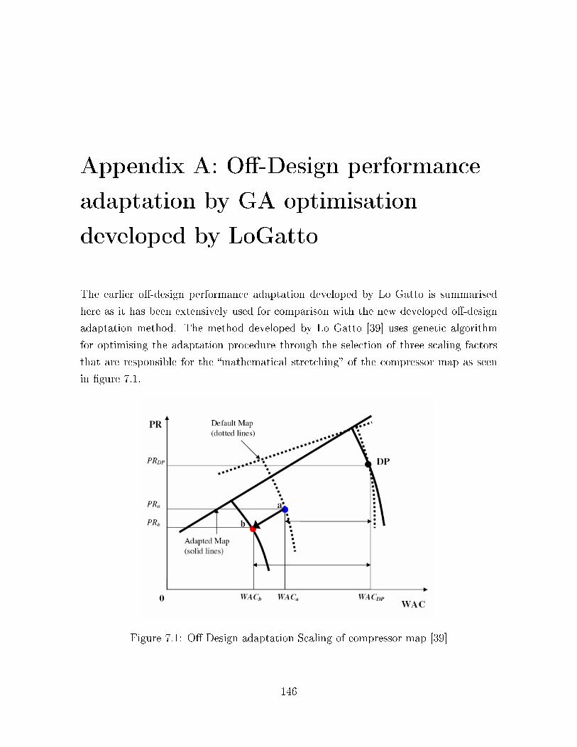
Appendix A: O�-Design performance

adaptation by GA optimisation

developed by LoGatto

The earlier o�-design performance adaptation developed by Lo Gatto is summarised

here as it has been extensively used for comparison with the new developed o�-design

adaptation method. The method developed by Lo Gatto [39] uses genetic algorithm

for optimising the adaptation procedure through the selection of three scaling factors

that are responsible for the �mathematical stretching� of the compressor map as seen

in �gure 7.1.

Figure 7.1: O�-Design adaptation Scaling of compressor map [39]

146

The design point for the default map and the adapted map is the same. The

o�-design operating point before adaptation labeled �a� and the operating point after

adaptation has been performed �b� corresponds to the adapted map and the point at

which all the target measurements have been matched.

The three o�-design scaling factors employed in this process are listed here:

SFPR,OD =PRb − PRDP

PRa − PRDP

(7.1)

SFWAC,OD =WACb −WACDP

WACa −WACDP

(7.2)

SFETA,OD =ETAb − ETADP

ETAa − ETADP

(7.3)

Therefore it can be said that each o�-design point at the adapted map is a function

of the distance between the initial point at the default map and the design point as

follows:

WACb = WACDP + (WACa −WACDP ) ∗ SFWAC,OD (7.4)

PRb = PRDP + (PRa − PRDP ) ∗ SFPR,OD (7.5)

ETAb = ETADP + (ETAa − ETADP ) ∗ SFETA,OD (7.6)

The optimisation procedure follows the same principles with the new developed

method, apart from the map generation method. The optimisation procedure is illus-

trated in �gure 7.2.

147

Figure 7.2: O�-Design Adaptation's Flow chart [39]

A series of test cases proved that this adaptation method developed by Lo Gatto is

a fast and accurate procedure for single point adaptation. In multiple point adaptation

test cases this approach lacks in terms of accuracy and this is mainly due to the nature

of the map scaling that is performed. This limitation has been overcome by the new

developed o�-design adaptation that incorporates a novel compressor map generation

method.

148

performance adaptation of gas turbines for power generation

Documents