performance and energy efficiency ... - electrical & computermilenka/docs/armend.thesis.pdf ·...

PERFORMANCE AND ENERGY EFFICIENCY OF COMMON COMPRES-

SION/DECOMPRESSION UTILITIES: AN EXPERIMENTAL STUDY IN MOBILE

AND WORKSTATION COMPUTER PLATFORMS

by

ARMEN A. DZHAGARYAN

A THESIS

Submitted in partial fulfillment of the requirements

for the degree of Master of Science in Engineering

in

The Department of Electrical & Computer Engineering

to

The School of Graduate Studies

of

The University of Alabama in Huntsville

HUNTSVILLE, ALABAMA

2013

ii

In presenting this thesis in partial fulfillment of the requirements for a master’s de-

gree from The University of Alabama in Huntsville, I agree that the Library of this

University shall make it freely available for inspection. I further agree that permis-

sion for extensive copying for scholarly purposes may be granted by my advisor or, in

his/her absence, by the Chair of the Department or the Dean of the School of Gradu-

ate Studies. It is also understood that due recognition shall be given to me and to

The University of Alabama in Huntsville in any scholarly use which may be made of

any material in this thesis.

(student signature) (date)

iii

THESIS APPROVAL FORM

Submitted by Armen A. Dzhagaryan in partial fulfillment of the requirements for

the degree of Master of Science in Engineering in Computer Engineering and ac-

cepted on behalf of the Faculty of the School of Graduate Studies by the thesis com-

mittee.

We, the undersigned members of the Graduate Faculty of The University of Ala-

bama in Huntsville, certify that we have advised and/or supervised the candidate on

the work described in this thesis. We further certify that we have reviewed the the-

sis manuscript and approve it in partial fulfillment of the requirements for the de-

gree of Master of Science in Engineering in Computer Engineering.

Committee Chair

(Date)

Department Chair

College Dean

Graduate Dean

iv

ABSTRACT

The School of Graduate Studies

The University of Alabama in Huntsville

Degree Master of Science in Engineering College/Dept. Engineering/Electrical &

Computer Engineering

Name of Candidate Armen A. Dzhagaryan

Title Performance and Energy Efficiency of Compression/Decompression

Utilities: An Experimental Study in Mobile and Workstation Computer Platforms

Lossless compression and decompression are routinely used in mobile and

workstation computer systems to reduce the costs of communicating and storing da-

ta. This research presents the results of a measurement-based experimental evalua-

tion of common compression and decompression utilities running on several plat-

forms of varying hardware complexity representing current mobile and workstation

systems. The evaluation involves characterization of the compression and decom-

pression utilities in a multi-dimensional space encompassing the compression ratio,

compression and decompression throughput, and energy efficiency. Different use

scenarios and conditioning typical for modern mobile and workstation computing

platforms are considered. The study observes a wide variety of energy costs associat-

ed with data compression and decompression and provides practical guidelines for

selecting the most energy efficient configurations for each system and use scenario

considered.

Abstract Approval: Committee Chair

Department Chair

Graduate Dean

v

ACKNOWLEDGMENTS

The work presented in this research would not be possible without the assis-

tance of a number of people who need to be acknowledged. Foremost, I would like to

thank my advisor, Dr. Aleksandar Milenkovic, for his initial experimental setup and

for his continuous counsel and support throughout the entire time. Second, I would

like to thank Mladen Milosevic who designed mPowerProfile. I relied on mPowerPro-

file in this research to acquire power traces from mobile platforms. Its features and

elegance saved me a lot of hours and made my journey more enjoyable.

Most importantly I would like to thank my family, my mother Irina and aunt

Svetlana, for their unconditional love and support. I am grateful for their encour-

agement and motivation in pursuing my academic goals.

vi

TABLE OF CONTENTS

Page

LIST OF FIGURES ...................................................................................................... xi

LIST OF TABLES ........................................................................................................ xv

CHAPTER

1 INTRODUCTION ...................................................................................................... 1

1.1 Background and Motivation ........................................................................... 1

1.2 Data Compression ........................................................................................... 3

1.3 What has been done? ...................................................................................... 4

1.4 Contributions .................................................................................................. 7

1.5 Thesis Outline ................................................................................................. 7

2 BACKGROUND ......................................................................................................... 9

2.1 Lossless Compression Utilities ....................................................................... 9

2.1.1 gzip ...................................................................................................11

2.1.2 lzop ...................................................................................................11

2.1.3 bzip2 .................................................................................................12

2.1.4 xz ......................................................................................................12

2.1.5 pigz ...................................................................................................13

2.1.6 pbzip2 ...............................................................................................13

2.2 Evaluated Computer Platforms .....................................................................13

vii

2.2.1 Pandaboard ......................................................................................13

2.2.2 Raspberry Pi ....................................................................................15

2.2.3 Workstation platform ......................................................................17

2.3 Operating Systems .........................................................................................18

2.3.1 Mobile Systems ................................................................................18

2.3.2 Workstation and Server Systems ....................................................19

2.4 Power Measurement and Profiling ................................................................20

2.4.1 Mobile Systems ................................................................................20

2.4.2 Desktop, Workstation and Server Systems .....................................21

3 RELATED WORK .....................................................................................................23

3.1 Mobile Systems ..............................................................................................23

3.2 Workstations and Servers .............................................................................25

4 EXPERIMENTAL SETUP ........................................................................................27

4.1 Experimental Goals .......................................................................................27

4.2 Metrics ...........................................................................................................27

4.2.1 Compression Ratio ...........................................................................28

4.2.2 Performance .....................................................................................28

4.2.3 Energy efficiency ..............................................................................29

4.3 Datasets .........................................................................................................30

4.4 Measurement setup .......................................................................................31

4.4.1 Measurement Setup for Mobile Platforms ......................................32

viii

4.4.1.1 Energy Calculation Example .............................................35

4.4.2 Workstation......................................................................................38

4.5 Experiments ...................................................................................................39

4.5.1 Frequency Scaling ............................................................................43

4.5.2 Idle Currents ....................................................................................44

4.5.3 Commands .......................................................................................45

5 PANDABOARD RESULTS .......................................................................................47

5.1 Compression Ratio .........................................................................................47

5.2 Compression and Decompression Throughputs ............................................48

5.2.1 Local .................................................................................................48

5.2.2 Wired ................................................................................................50

5.2.3 Wireless ............................................................................................53

5.3 Energy Efficiency ...........................................................................................55

5.3.1 Local .................................................................................................55

5.3.2 Wired ................................................................................................59

5.3.3 Wireless ............................................................................................62

5.4 Frequency scaling ..........................................................................................65

5.4.1 Local .................................................................................................66

5.4.1.1 Compression and Decompression Throughputs ................66

5.4.1.2 Energy Efficiency ...............................................................69

5.4.2 Wired ................................................................................................73

ix



5.4.3 Wireless ............................................................................................80



5.5 Conclusions ....................................................................................................86

6 RASPBERRY PI RESULTS ......................................................................................91

6.1 Compression ratio ..........................................................................................91

6.2 Compression and Decompression Throughputs ............................................91

6.2.1 Local .................................................................................................91

6.2.2 Wired ................................................................................................93

6.3 Energy Efficiency ...........................................................................................95

6.3.1 Local .................................................................................................95

6.3.2 Wired ................................................................................................99

6.4 Conclusions .................................................................................................. 102

7 WORKSTATION RESULTS ................................................................................... 106

7.1 Compression ratio ........................................................................................ 106

7.2 Compression and Decompression Throughputs .......................................... 107

7.2.1 Local ............................................................................................... 107

7.2.2 Wired .............................................................................................. 109

7.3 Energy Efficiency ......................................................................................... 111

x

7.3.1 Local ............................................................................................... 111

7.3.2 Wired .............................................................................................. 115

7.4 Frequency scaling ........................................................................................ 119

7.4.1 Local ............................................................................................... 120

7.4.1.1 Compression and Decompression Throughputs .............. 120

7.4.1.2 Energy Efficiency ............................................................. 124

7.4.2 Wired .............................................................................................. 126

7.4.2.1 Compression and Decompression Throughputs .............. 126

7.4.2.2 Energy Efficiency ............................................................. 130

7.5 Conclusions .................................................................................................. 132

8 CONCLUSIONS...................................................................................................... 136

REFERENCES .......................................................................................................... 139

xi

LIST OF FIGURES

Figure Page

2.1 Pandaboard ...........................................................................................................14

2.2 Raspberry Pi ..........................................................................................................16

4.1 Measurement Setup for Pandaboard and Raspberry Pi ......................................33

4.2 mPowerProfile software ........................................................................................34

4.3 Sample File Example ............................................................................................36

4.4 Current drawn by Pandaboard during execution on gzip utility .........................37

4.5 likwid-powermeter gzip -1 example ......................................................................39

4.6 write_null in Linux kernel source code for /dev/null ............................................40

4.7 Experimental data flow .........................................................................................42

4.8 cpufreq-info output ................................................................................................43

4.9 Commands for the Local experiment ....................................................................45

4.10 Commands for the Wired and Wireless experiments .........................................46

5.1 Pandaboard and Raspberry Pi: Compression Ration (totalInput.tar) .................48

5.2 Pandaboard: Local Compression/Decompression Throughput ............................49

5.3 Pandaboard: Wired Compression/Decompression Throughput ...........................52

5.4 Pandaboard: Wireless Compression/Decompression Throughput .......................54

5.5 Pandaboard: Local Energy Efficiency for Compression .......................................57

5.6 Pandaboard: Local Energy Efficiency for Decompression ....................................58

5.7 Pandaboard: Wired Energy Efficiency for Compression ......................................60

5.8 Pandaboard: Wired Energy Efficiency for Decompression...................................61

5.9 Pandaboard: Wireless Energy Efficiency for Compression ..................................63

5.10 Pandaboard: Wireless Energy Efficiency for Decompression ............................65

xii

5.11 Pandaboard: Local Compression Throughput under Different Frequencies

(MB/sec) ........................................................................................................................67

5.12 Pandaboard: Local Decompression Throughput under Different Frequencies

(MB/sec) ........................................................................................................................67

5.13 Pandaboard: Local Throughput Ratios and Frequency Ratios ..........................69

5.14 Pandaboard: Local Energy Efficiency for Compression under Different

Frequencies ..................................................................................................................70

5.15 Pandaboard: Local Energy Efficiency for Decompression under Different

Frequencies ..................................................................................................................72

5.16 Pandaboard: Wired Compression Throughput under Different Frequencies ....73

5.17 Pandaboard: Wired Decompression Throughput under Different Frequencies 74

5.18 Pandaboard: Wired Throughput Ratios and Frequency ratios ..........................75

5.19 Pandaboard: Wired Energy Efficiency for Compression under Different

Frequencies ..................................................................................................................77

5.20 Pandaboard: Wired Energy Efficiency for Decompression under Different

Frequencies ..................................................................................................................79

5.21 Pandaboard: Wireless Compression Throughput under Different Frequencies 80

5.22 Pandaboard: Wireless Decompression Throughput under Different Frequencies

......................................................................................................................................81

5.23 Pandaboard: Wireless Throughput Ratios and Frequency Ratios .....................82

5.24 Pandaboard: Wireless Energy Efficiency for Compression under Different

Frequencies ..................................................................................................................84

5.25 Pandaboard: Wireless Energy Efficiency for Decompression under Different

Frequencies ..................................................................................................................86

6.1 Raspberry Pi: Local Compression/Decompression Throughput ...........................92

xiii

6.2 Raspberry Pi: Wired Compression/Decompression Throughput ..........................93

6.3 Raspberry Pi: Local Energy Efficiency for Compression ......................................97

6.4 Raspberry Pi: Local Energy Efficiency for Decompression ..................................98

6.5 Raspberry Pi: Wired Energy Efficiency for Compression .................................. 100

6.6 Raspberry Pi: Wired Energy Efficiency for Decompression ............................... 102

7.1 Workstation: Compression Ratio ........................................................................ 107

7.2 Workstation: Local Compression/Decompression Throughput (MB/sec)

(enwik9.xml) ............................................................................................................... 108

7.3 Workstation: Wired Compression/Decompression Throughput (enwik9.xml) .. 110

7.4 Workstation: Local Energy Efficiency for Compression (enwik9.xml) .............. 113

7.5 Workstation: Local Energy Efficiency for Decompression (enwik9.xml) ........... 115

7.6 Workstation: Wired Energy Efficiency for Compression (enwik9.xml) ............. 117

7.7 Workstation: Wired Energy Efficiency for Decompression (MB/Joule)

(enwik9.xml) ............................................................................................................... 119

7.8 Workstation: Local Compression Throughput under Different Frequencies

(MB/sec) (enwik9.xml) ............................................................................................... 121

7.9 Workstation: Local Decompression Throughput under Different Frequencies

(MB/sec) (enwik9.xml) ............................................................................................... 121

7.10 Workstation: Local Compression Throughput Ratios vs. Frequency Ratios

(enwik9.xml) ............................................................................................................... 123

7.11 Workstation: Local Decompression Throughput Ratios vs. Frequency Ratios

(enwik9.xml) ............................................................................................................... 124

7.12 Workstation: Local Energy Efficiency for Compression under Different

Frequencies (MB/Joule) (enwik9.xml) ....................................................................... 125

xiv

7.13 Workstation: Local Energy Efficiency for Decompression under Different


7.14 Workstation: Wired Compression Throughput under Different Frequencies

(MB/sec) (enwik9.xml) ............................................................................................... 127

7.15 Workstation: Wired Decompression Throughput under Different Frequencies

(MB/sec) (enwik9.xml) ............................................................................................... 128

7.16 Workstation: Wired Compression Throughput Ratios vs. Frequencies Ratios

(enwik9.xml) ............................................................................................................... 129

7.17 Workstation: Wired Decompression Throughput Ratios vs. Frequency Ratios

(enwik9.xml) ............................................................................................................... 130

7.18 Workstation: Wired Energy Efficiency for Compression under Different


7.19 Workstation: Wired Energy Efficiency for Decompression under Different


xv

LIST OF TABLES

Table Page

2.1 Lossless Compression Utilities ..............................................................................10

4.1 Dataset – totalInput.tar .........................................................................................31

4.2 Datasets Summary .................................................................................................31

4.3 Idle Currents for Pandaboard and Raspberry Pi ..................................................44

5.1 Throughputs on Pandaboard @ 1.01GHz .............................................................87

5.2 Energy Efficiency on Pandaboard @ 1.01GHz ......................................................88

5.3 Performance Gains of Parallel Utilities on Pandaboard @ 1.01GHz ....................89

6.1 Throughputs on Raspberry Pi @ 700MHz .......................................................... 103

6.2 Energy Efficiency on Raspberry Pi @ 700MHz ................................................... 104

6.3 Performance Gain of Parallel Utilities on Raspberry Pi @ 700MHz .................. 105

7.1 Throughputs on Workstation @ 3.40GHz ........................................................... 133

7.2 Energy Efficiency on Workstation @ 3.40GHz ................................................... 134

7.3 Performance Gains of Parallel Utilities on Workstation @ 3.40GHz.................. 134

1

CHAPTER 1

INTRODUCTION

An exponential growth of the Internet traffic and emergence of mobile com-

puting platforms with limited storage and energy resources make data compression

and decompression crucial as they can reduce communication latencies and make

effective use of the available storage. A number of compression utilities have been

developed and routinely used in many areas of computing. In this thesis we focus on

lossless compression and decompression, critical for all non-audio or non-video based

digital content. Whereas common lossless compression and decompression utilities

are well-understood as far as their performance and compression ratios are consid-

ered, little is known about their energy efficiency. The goal of this thesis is explore

energy-efficiency of common utilities in typical use scenarios of mobile and desktop

computing. The rest of the Introduction section gives background and motivation,

discusses data compression, describes work done in the thesis, lists contributions of

this thesis, and gives the outline of the rest of the thesis.

1.1 Background and Motivation

The total number of computing devices has been increasing substantially in

recent years, mainly due to unprecedented proliferation of mobile computing devices.

Mobile devices such as smartphones, tablet computers, and e-readers have steadily

been gaining market share, dethroning laptop and desktop computers as dominant

personal computing platforms. According to an estimate for 2011 [1], vendors

2

shipped 487.7 million smartphones (up 63% from the year before) and 67 million tab-

lets (up 274%), whereas the number of notebooks and desktop computers shipped

was 209.6 million (up 7.5%) and 112.4 million (up 2.3%), respectively. A more recent

estimates report a record 700 million smartphones shipped (up 43% from the year

before) in 2012 [2], and 383 million of personal and desktop computers (notebooks

and desktop computers combined) was estimated to be sold [3]. It is forecasting that

the number of smartphones and tablets shipped in 2015 will reach 1.4 billion and

326 million, respectively [1], whereas the number of personal computers shipped in

2015 will reach 490.6 million [3].

The amount of data traffic initiated from mobile devices has been growing

rapidly as well. A report from Cisco states that the global data traffic for mobile de-

vices alone grew 2.3-fold in 2011, reaching 597 petabytes per month, which is over 8

times greater than the total Internet traffic in 2000 [4].

Energy efficiency is becoming an important design requirement for mobile

and workstation platforms alike. For mobile devices, it is driven by several key fac-

tors, including (i) limited energy capacity of batteries, (ii) cost considerations favor-

ing less expensive packaging, and (iii) user convenience favoring lightweight designs

with small form factors that operate for long periods without battery recharges. For

workstations and servers, it is driven specifically by the desire to reduce the operat-

ing costs of data centers. However, the greener outlook on energy consumption is al-

so taken often by device manufacturers of desktop, laptop, and ultrabook computers.

With current trends, where data traffic is increasing and large consumption

of digital information is observed on mobile devices with limited storage and energy

resources, minimizing storage capacity requirements and energy costs of data com-

munication is of great interest for both mobile devices and workstations in data cen-

3

ters that make consumption of data available. Data compression utilities are thus

critical in achieving energy-efficient data communication, reducing communication

latencies and making effective use of available storage.

1.2 Data Compression

The general goal of data compression is to reduce the number of bits needed

to represent information. Data can be compressed losslessly or lossily. Lossless com-

pression means that the original data can be reproduced exactly by the decompres-

sor. In contrast, lossy compression, which often results in much higher compression

ratios, can only approximate the original data. This is typically acceptable if the da-

ta are meant for human consumption such as audio and video. However, program

code input, medical data, email and other text do not tolerate lossy compression.

This thesis focuses on lossless compression only for this research.

Lossless compression is achieved by replacing frequent bit or byte strings

with shorter sequences and infrequent bit or byte strings with longer sequences,

which tends to reduce the overall data size. For example, in Huffman compression,

bit strings are assigned unique, variable-length code words whose length is inversely

proportional to the frequency of the corresponding bit strings. Huffman coding [5], or

the slower but more sophisticated arithmetic coding [6], is often preceded by a trans-

formation stage whose purpose it is to model (or predict) the data. If the model is

good, i.e., accurate, then the difference sequence between the predicted and the ac-

tual data primarily consists of small values that cluster around zero, which are easy

to encode effectively. Various models are in use, including dictionaries of expected or

recently encountered “words,” sliding windows that assume that recently seen data

patterns will repeat, which are used in the Lempel-Ziv approach [7], as well as re-

4

versibly sorting data to bring similar values close together, which is the approach

taken by the Burrows and Wheeler transform [8]. The data compression algorithms

used in practice combine different models and coders, thereby favoring different

types of inputs and representing different tradeoffs between speed and compression

ratio. Moreover, they typically allow the user to select the dictionary, window, or

block size through a command-line argument.

The choice of algorithm, compression level, and the quality of the implemen-

tation also affect the energy consumption. This aspect is not critical on desktop PCs

and workstations, but it can be a decisive factor in battery-powered handheld devic-

es. In fact, it is reasonable to assume that achieving a higher compression ratio re-

quires more computation and therefore energy, but better compression reduces the

number of bytes, thus saving energy when transmitting the data. Hence, it is benefi-

cial to take a close look at the energy-efficiency of lossless compression algorithms

across systems of varies hardware complexity, such as state-of-the-art mobile and

workstation platforms that communicates over the network. In particular, answers

to whether compression is useful for reducing energy consumption, which common

compression algorithms should be used, what configurations result in the best ener-

gy efficiency, and whether parallel execution can save energy are needed.

1.3 What has been done?

In this thesis, a comparative study of the most recent versions of several pop-

ular compression utilities, including gzip, lzop, bzip2, xz, pigz (a parallel implemen-

tation of gzip) and pbzip2 (a parallel implementation of bzip2) are performed on sev-

eral contemporary computing platforms. Platforms include Pandaboard, a state-of-

the-art mobile development platform, Raspberry Pi, a low-end mobile computer plat-

5

form, and a Dell Precision T1600 workstation. For each utility, the effectiveness of

all supported compression levels is analyzed to provide a complete picture. Common

performance metrics such as compression ratio and compression and decompression

throughputs are examined. Energy-efficiency metrics are introduced and the energy

consumed by compression and decompression tasks is studied using our experi-

mental setup for energy measurements. To study effects of frequency scaling on

Pandaboard and the workstation platform, the experiments are repeated for each

frequency step. Pandaboard supports four frequency steps, 300MHz, 600MHz,

800MHz and 1.01GHz. The workstation platform supports ten frequency steps for

each core from 1.60GHz to 3.40GHz.

The compression utilities evaluated in three typical use scenarios. The Local

experiment involves compression and decompression tasks performed locally on sys-

tem under test (Pandaboard/Raspberry Pi/Workstation). The Wired and Wireless

experiments involve compression tasks that stream data to and from a remote server

over a secure communication channel. The Wired experiment uses an Ethernet net-

work interface, and the Wireless experiment uses a wireless LAN interface. Com-

pression utilities for Raspberry Pi and Workstation are evaluated only for the Local

and Wired experiment for reasons of not having native wireless adapter. Only Pan-

daboard, with single-chip platform WiLink™ 6.0 provides wireless LAN natively [9].

The main findings of research are as follows.

The effectiveness of compression utilities varies widely across different

utilities and compression levels, often spanning two orders of magnitude.

For local compression and compression with upload over the wired net-

work, the fastest utility, lzop with compression levels -1 to -6, performs

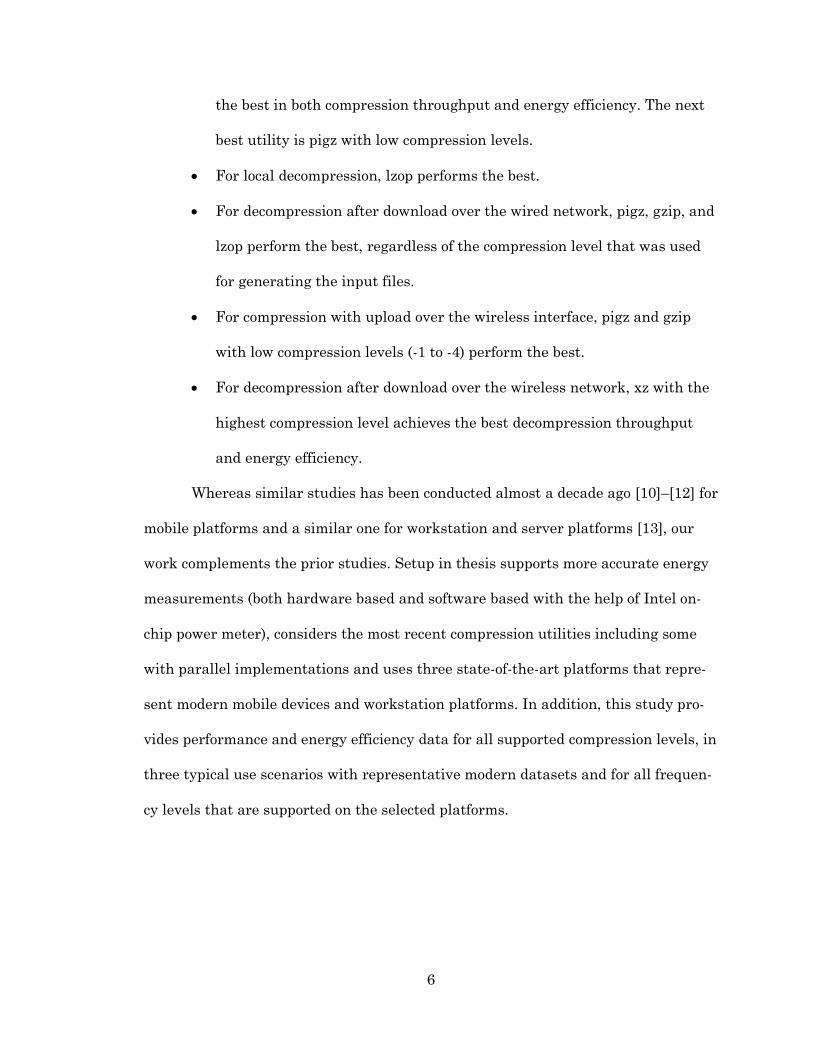
6

the best in both compression throughput and energy efficiency. The next

best utility is pigz with low compression levels.

For local decompression, lzop performs the best.

For decompression after download over the wired network, pigz, gzip, and

lzop perform the best, regardless of the compression level that was used

for generating the input files.

For compression with upload over the wireless interface, pigz and gzip

with low compression levels (-1 to -4) perform the best.

For decompression after download over the wireless network, xz with the

highest compression level achieves the best decompression throughput

and energy efficiency.

Whereas similar studies has been conducted almost a decade ago [10]–[12] for

mobile platforms and a similar one for workstation and server platforms [13], our

work complements the prior studies. Setup in thesis supports more accurate energy

measurements (both hardware based and software based with the help of Intel on-

chip power meter), considers the most recent compression utilities including some

with parallel implementations and uses three state-of-the-art platforms that repre-

sent modern mobile devices and workstation platforms. In addition, this study pro-

vides performance and energy efficiency data for all supported compression levels, in

three typical use scenarios with representative modern datasets and for all frequen-

cy levels that are supported on the selected platforms.

7

1.4 Contributions

This thesis makes the following contributions to the field of measurement-

based power profiling and to the field of compression and decompression on mobile

and workstation platforms:

Providing an accurate performance and energy efficiency evaluation of

modern compression and decompression utilities on three platforms that

represent three distinct types of today’s computer hardware: mobile de-

vices, low-end devices, and workstations and servers.

Evaluating the effects of frequency scaling on performance and energy-

efficiency across all compression levels.

Creating experimental environment for measurement-based energy profil-

ing of the program running on mobile computing platforms.

Creating experimental methods for energy profiling of programs running

on a workstation and server computers.

1.5 Thesis Outline

The rest of thesis is organized as follows. Chapter 2 gives background on this

research, including compression algorithms and utilities, mobile platforms, and

power profiling. Chapter 3 presents related work by highlighting relevant studies

performed in similar conditions. Chapter 4 specifies the experimental goals, metrics,

datasets, measurement setup, and experiments conducted. Chapters 5, 6 and 7 dis-

cuss the results for each selected computing device, Pandaboard, Raspberry Pi, and

the workstation, respectively. Chapter 8 summarizes the thesis, draws conclusions

for all three platforms together, and gives suggestions for future work in the area of

this study.

9

CHAPTER 2

BACKGROUND

This chapter covers background on several aspects of this research. Section

2.1 gives details on selected lossless compression utilities and their algorithms to

provide understanding on how selected lossless compression utilities work at the

basic level. Section 2.2 discusses each of the three computer platforms selected for

evaluation, highlighting both hardware and software specifications of each. Section

2.3 discuses operating systems selection on both mobile and workstation computers.

Section 2.4 discusses related work in power profiling.

2.1 Lossless Compression Utilities

The use of lossless compression can be found in various software distributions

systems of Linux distributions, and Apple and Android app stores. For example, two

most popular software package formats used in number of different Linux distribu-

tions are .deb (used in Debian based distributions) and .rpm (used in Red Hat based

distributions). Those two packages contain application data that is retrieved from

software repositories, and their content can be optional compressed with gzip, bzip2,

lzma and xz. For app stores used in iOS and Android devices, .ipa and .apk file ex-

tensions are used for distribution of applications. Both file extensions are based on

zip file format with various other extensions, such as encryption, and system specific

(iOS or Android) structure built on top.

10

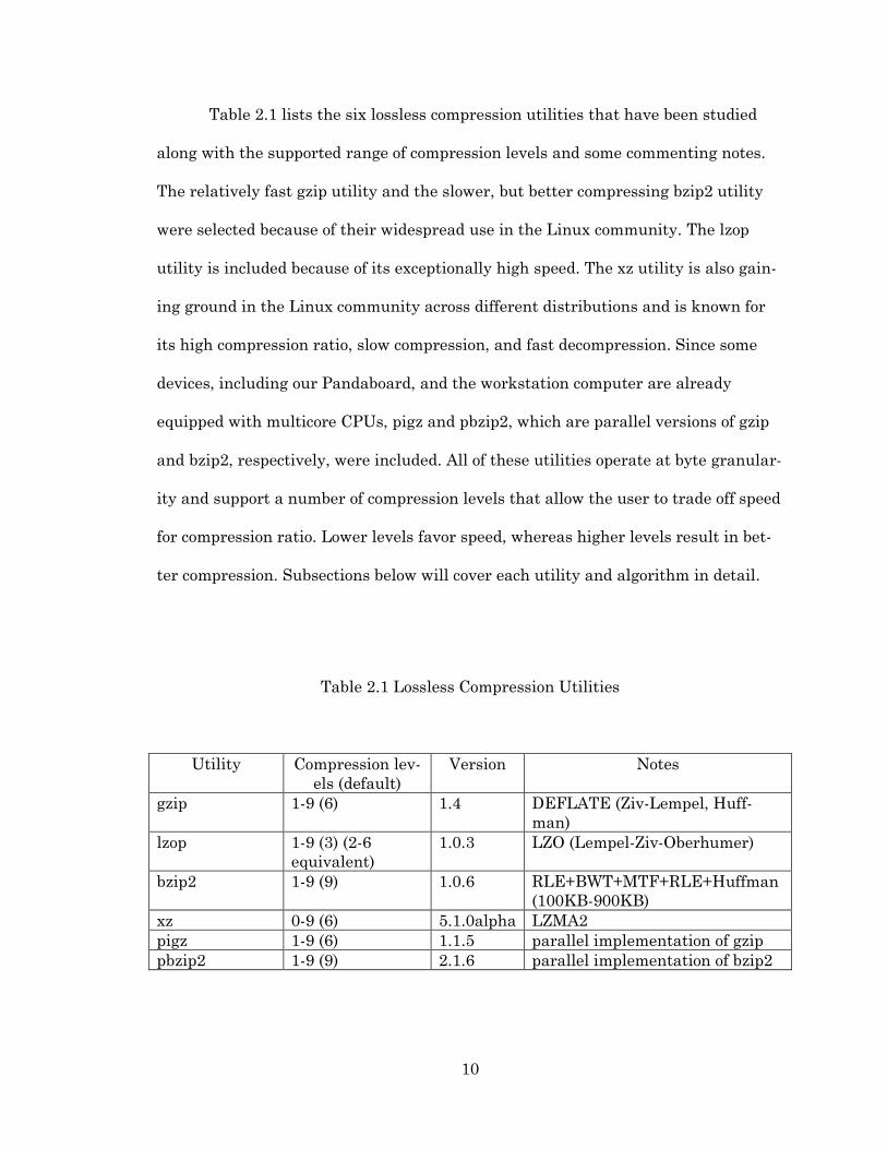
Table 2.1 lists the six lossless compression utilities that have been studied

along with the supported range of compression levels and some commenting notes.

The relatively fast gzip utility and the slower, but better compressing bzip2 utility

were selected because of their widespread use in the Linux community. The lzop

utility is included because of its exceptionally high speed. The xz utility is also gain-

ing ground in the Linux community across different distributions and is known for

its high compression ratio, slow compression, and fast decompression. Since some

devices, including our Pandaboard, and the workstation computer are already

equipped with multicore CPUs, pigz and pbzip2, which are parallel versions of gzip

and bzip2, respectively, were included. All of these utilities operate at byte granular-

ity and support a number of compression levels that allow the user to trade off speed

for compression ratio. Lower levels favor speed, whereas higher levels result in bet-

ter compression. Subsections below will cover each utility and algorithm in detail.

Table 2.1 Lossless Compression Utilities

Utility Compression lev-

els (default)

Version Notes

gzip 1-9 (6) 1.4 DEFLATE (Ziv-Lempel, Huff-

man)

lzop 1-9 (3) (2-6

equivalent)

1.0.3 LZO (Lempel-Ziv-Oberhumer)

bzip2 1-9 (9) 1.0.6 RLE+BWT+MTF+RLE+Huffman

(100KB-900KB)

xz 0-9 (6) 5.1.0alpha LZMA2

pigz 1-9 (6) 1.1.5 parallel implementation of gzip

pbzip2 1-9 (9) 2.1.6 parallel implementation of bzip2

11

2.1.1 gzip

gzip [14] implements the deflate algorithm, which is a variant of the LZ77 al-

gorithm [7]. It looks for repeating strings, i.e., sequences of bytes, within a 32 kB

sliding window. The length of the string is limited to 256 bytes. gzip uses two Huff-

man trees, one to compress the distances in the sliding window and another to com-

press the lengths of the strings as well as the individual bytes that were not part of

any matched sequence. The algorithm finds duplicated strings using a chained hash

table that is indexed with 3-byte strings. The selected compression level determines

the maximum length of the hash chains, and whether lazy evaluation should be

used. The evaluated version of gzip is 1.4.

2.1.2 lzop

lzop [15] uses LZO block-based compression algorithm that favors speed over

compression ratio and requires little memory to operate. It splits each block of data

into sequences of matches (a sliding dictionary) and non-matching literals, which it

then compresses. LZO requires no memory for decompression and requires only

64kB for compression. The speed for lzop is IO-bound and not CPU-bound. LZO al-

gorithm provides support for a wide range of systems both legacy and new.

The lzop utility stores original file name, ownership, mode and time stamp of

files during compression, allowing files to be restored in their original form when

decompressed. Compression levels are divided into three groups. The first group in-

cludes compression levels -2, -3, -4, -5 and -6 and offers fast compression. The second

group includes compression level -1 and it can be sometimes faster than the first

group. The last group that includes compression levels -7, -8, and -9 provide the best

compression ratio but with slower execution. Several standard switches are used to

12

turn on different options: -f forces compression or decompression, -c redirects output

to a specified location, -d indicates decompression, and –k keeps the original file. No

native parallel version of lzop currently exists, however process-level parallelism can

be used when using GNU Parallel tool with lzop. The evaluated version of lzop is

1.0.3.

2.1.3 bzip2

bzip2 [16] implements a variant of the block-sorting algorithm described by

Burrows and Wheeler (BWT) [8]. bzip2 applies a reversible transformation to a block

of inputs, uses sorting to group bytes with similar contexts together, and then com-

presses them with a Huffman coder. The selected compression level adjusts the

block size between 100 kB (with compression level -1) and 900 kB (with compression

level -9). The evaluated version of bzip2 is 1.0.6.

2.1.4 xz

xz [17] is based on the Lempel-Ziv-Markov chain compression algorithm

(LZMA) developed for 7-Zip [18]. It uses a large dictionary to achieve good compres-

sion ratios and employs a variant of LZ77 with special support for repeated match

distances. The output is encoded with a range encoder, which uses a probability

model for each bit (rather than whole bytes) to avoid mixing unrelated bits, i.e., to

boost the compression ratio. The evaluated version of xz is v5.1.0alpha. For Panda-

board and Raspberry Pi, xz was evaluated only with compression levels -0 through -6

as the memory requirement for levels -7 to -9 exceeds the available memory on those

platforms. For the workstation platform, this problem does not exist, and all com-

pression levels of xz are evaluated.

13

2.1.5 pigz

pigz [19] is a parallel version of gzip for shared memory machines which is

based on pthreads. It breaks the input up into 128 kB chunks and concurrently com-

presses multiple chunks. The compressed data are outputted in their original order.

Decompression operates mostly sequentially, however separate threads are created

for reading and writing [19]. The evaluated version of pigz is v1.1.5.

2.1.6 pbzip2

pbzip2 [20] is a multithreaded version of bzip2 that is based on pthreads. It

works by compressing multiple blocks of data simultaneously. The resulting blocks

are then concatenated to form the final compressed file, which is compatible with

bzip2. Decompression is also parallelized. The evaluated version of pbzip2 is 2.1.6.

2.2 Evaluated Computer Platforms

For this research, three platforms with varying hardware complexity are se-

lected so that the gained results and insights can have a wide application across

many current mobile and workstation platforms. Pandaboard and Raspberry Pi are

selected to represent typical mobile devices, and the workstation computer is select-

ed to represent workstations and servers based on the state-of-the-art processors

such as Sandy Bridge or Ivy Bridge [21].

2.2.1 Pandaboard

Pandaboard (Figure 2.1) is designed by Texas Instruments to support soft-

ware development for smartphones and other mobile devices [22]. It features a Tex-

as Instruments system-on-a-chip (SoC) OMAP4430 [23] with 1 GB of low-power

DDR2 SDRAM. The OMAP4430 SoC includes a dual-core ARM Cortex-A9 MPCore

processor, a 3D graphics accelerator, an image signal processor, and a rich set of

14

standard peripherals (timers, communication interfaces, and a memory controller).

A number of commercial mobile devices, such as Amazon Kindle Fire, BlackBerry

Playbook, Motorola Droid RAZR, Samsung Galaxy Tab and Galaxy S II, are based

on this chipset. Pandaboard also features an onboard 10/100 Ethernet port, a wire-

less interface (802.11 and Bluetooth), DVI and HDMI video interfaces, an audio in-

terface, and two USB ports.

Figure 2.1 Pandaboard

The platform can run various mobile open-source operating systems based on

the Linux kernel, including Ubuntu, Android, and MeeGo/Tizen. For experiments,

Ubuntu distribution provided by Linaro, a non-profit organization that works on

consolidating and optimizing open-source code for the ARM architecture [24], is se-

OMAP4430 (1 GHz dual-core ARM Cortex A9 + 3D graphics accelerator)1 GB DDR2

WLAN/Bluetooth

HDMI/DVI outputUSB10/100 Ethernet

Serial/RS232

SD/MMC card slot

PowerinputAudio

15

lected. Linaro provides both Android and Ubuntu for Pandaboard platform; however,

the Ubuntu build is much more stable and provides more flexibility and control. One

goal for performing highly representative measurements of compression or decom-

pression on the selected platform was to have the ability to turn off any unrelated

tasks in the system. With Linux, it was possible to kill all potentially results affect-

ing tasks. This includes shutting down graphical desktop enlivenment, disabling

network daemons when they are not in use (e.g, in experiments that do not involve

network communication). Ubuntu and Linux are also gaining ground in the mobile

systems. Canonical, a company that leads the development of Ubuntu announced

their plans to enter the mobile market by demonstrating Ubuntu for phones, a

standalone operating system for mobile devices. They plan to offer a full access to

desktop operating system on smartphones, when they are docked with monitor and

I/O devices. In addition, the Android, the most popular platform on smartphones re-

lies on the Linux kernel.

2.2.2 Raspberry Pi

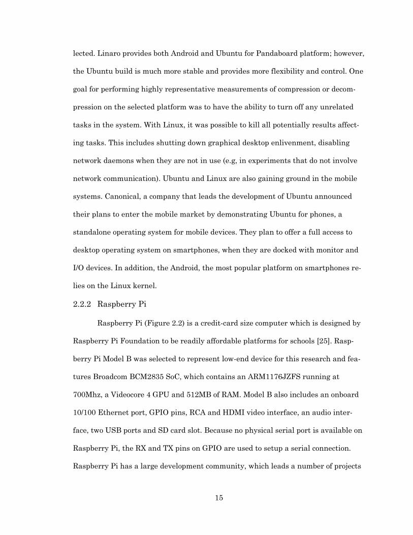
Raspberry Pi (Figure 2.2) is a credit-card size computer which is designed by

Raspberry Pi Foundation to be readily affordable platforms for schools [25]. Rasp-

berry Pi Model B was selected to represent low-end device for this research and fea-

tures Broadcom BCM2835 SoC, which contains an ARM1176JZFS running at

700Mhz, a Videocore 4 GPU and 512MB of RAM. Model B also includes an onboard

10/100 Ethernet port, GPIO pins, RCA and HDMI video interface, an audio inter-

face, two USB ports and SD card slot. Because no physical serial port is available on

Raspberry Pi, the RX and TX pins on GPIO are used to setup a serial connection.

Raspberry Pi has a large development community, which leads a number of projects

16

ranging from entertainment centers to dedicated computers for photography, home

automation, medical and robotic fields. Raspberry Pi Foundation has sold close to a

million devices [25] in less than a year since it has been introduced.

Figure 2.2 Raspberry Pi

Raspberry Pi supports several Linux distributions, including Debian [26],

Arch [27] and several distributions built around XBMC (Xbox Media Center) such as

Raspbmc and OpenELEC [28], [29]. Additionally, there are projects to provide sup-

port for Android operating system [30]. In this research, a Debian for Raspberry Pi

is used.

RCA Video out Audio out

USB 2.0

Ethernet

GPIO Headers

Broadcom BCM2835 ARM11 (700 MHz)

SD card slot(back side)

HDMI

MicroUSB

17

2.2.3 Workstation platform

For the workstation platform, a Dell Precision T1600 workstation is used. It

features a quad-core Intel Xeon CPU E31270 processor based on Sandy Bridge ar-

chitecture. Each processor core supports 2-way multithreading; thus the total num-

ber of logical processor cores is eight. The processor chip supports ten frequency

steps ranging from 1.60GHz to 3.40GHz. It features a three-level cache system, with

256KB L1 data cache, 1 MB L2 cache, and 8 MB L3 cache. The system memory is

8GB DIMM DDR3 synchronous at 1333MHz (0.8ns). The secondary storage includes

an ATA hard disk with capacity of 1 TB. The workstation includes a gigabit network

interface, a USB controller, audio and video interfaces, including NVIDIA Quadro

GF106GL PCI Express graphics card.

The selected workstation allows the use of likwid lightweight performance

tools to perform power measurement, specifically likwid-powermeter which will be

discussed in details in Chapter 4. The Intel Xeon E31270 processor includes -- an on-

chip resource for estimating energy and power of running tasks using events record-

ed in performance monitoring registers and their proprietary model that captures

physical characteristics of the processor. The likwid tool interfaces the power meter

and outputs power measurements in joules and watts. Intel researchers demon-

strated that this on-chip resource gives estimates for the energy and power that are

within several percentages of those acquired by the actual power measurements

[21].

The workstation supports any operating system built to support i386 or

x86_64 architecture. For this research, Ubuntu 12.04 was used to be consistent with

experimental methods on other systems under test (Pandaboard and Raspberry Pi).

18

2.3 Operating Systems

This section gives a brief overview of operating systems for mobile and work-

station platforms, and describes reasons for selecting Linux as the primary operat-

ing system for performing experiments across all selected systems in this research.

2.3.1 Mobile Systems

On mobile systems, two most popular operating systems are iOS from Apple,

and Android from Google. Android and iOS capture 92% of the global smartphone

shipments in Q4 of 2012 as reported by Strategy Analytics [31]. Similar market

share is observed for both operating systems on tablets. The smaller market share is

taken by Microsoft with their Windows Mobile and Windows 8 on smartphones and

tablets. In addition to these three, there are other mobile operating systems that are

either in development or command a much smaller market share. One example is

Tizen [32], funded and developed by Linux Foundation, Samsung and Intel (a previ-

ous project MeeGo [33]). WebOS was converted by HP from a failed mobile attempt

to an open source mobile project [34]. Firefox also recently started to develop a

HTML5 based operating system with their Firefox OS [35]. Finally, Canonical, the

group behind Ubuntu operating system, the most popular Linux distribution on

desktops have introduced their mobile OS for mobile phones at Consumer Electron-

ics Show (CES) of 2013 [36]. It is important to note that Ubuntu, in comparison with

the majority of other mobile operating system, including iOS and Android, is offering

the same operating system to be used across both mobile and computer devices, and

proposing an idea of using powerful smartphone devices as full-desktop systems once

they are docked to a special docking station connected to a monitor, keyboard, mouse

and other I/O [37].

19

The majority of above mentioned operating system, excluding iOS and Win-

dows Mobile or Windows 8, share a common feature of utilizing Linux kernel at their

core. This indicates that anything that can work well on a basic level on Linux dis-

tribution (for example compression or decompression) will work well on the majority

of mobile operating systems, including Android. This was one of the reasons why a

Linux distribution (with the majority of unrelated tasks turned off) is selected to

perform all measurement tests. This provided clean and reliable measurements and

results that can be applied not only to Ubuntu, but easily to Android, Tizen, Firefox

OS and other Linux based mobile operating systems. Another reason for using

Linux, instead of Android, was better integration on development platforms and

higher flexibility on controlling (turning off) running tasks.

2.3.2 Workstation and Server Systems

Linux is used on desktop, workstations and server systems across house-

holds, businesses and data centers. Linux is increasingly used in datacenters and

server farms with w3tech reports that Linux is used in 32.8% of webservers [38].

Major companies such as Lenovo, Dell, IBM and HP are offering certified hardware

[39] for various Linux distributions. New Linux-powered consumer products such as

TV media centers [40] and gaming consoles [41] [42] are emerging. Those reasons

were behind the choice of selecting Ubuntu Linux distribution as operating system

for all performance and power measurement tests in this research. Similarly to mo-

bile systems, Linux was also selected due to its higher flexibility and controllability.

20

2.4 Power Measurement and Profiling

This section discusses previous studies in the field of power measurement

and profiling. Subsection 2.4.1 and Subsection 2.4.2 cover information for mobile and

workstation systems, respectively.

2.4.1 Mobile Systems

There are a number of different studies that explore and seek for new ways of

manage or reduce power consumption on mobile devices. This is motivated by lim-

ited battery operating time and consumers’ demand for longer single charge mobile

use. The proposed solutions on managing mobile power consumption include

schemes with cloud offloading [43] [44], run-time power modeling [45] [46] [47], and

energy estimation [48], [49].

Carroll and Heiser try to understand which component in today’s typical mo-

bile device are the biggest energy consumer by performing direct energy measure-

ment [48]. They measured the energy consumed by individual components including

CPU, RAM memory, flash storage, network and GPS. They evaluate different usage

scenarios and applications such as audio playback, video playback, text messaging,

phone calls, emailing and web browsing. The paper concluded that the majority of

power consumption can be attributed to network communication and display. Their

experimental setup, similar to the setup used in this thesis, consisted of using DAQ

from National Instruments and a sense resistors inserted at the power supply rails

to measure voltage drops across resistor, which is used for calculation of power and

energy.

Bircher and John estimate system power consumption using processor per-

formance events [49]. The complete list of performance events included cycles, halted

21

cycles, fetched micro-operations, L3 Cache misses, TLB misses, DMA accesses, pro-

cessor memory bus transactions, un-cacheable accesses and interrupts. Analysis of

performance events offline using software tools provided models and formulas for

accurate power estimation for CPU, memory, disk and I/O. Accuracy of their method

was demonstrated by synchronous comparison of estimations with direct hardware

measurements. Downside to their study is the hardware dependent models and for-

mulas, requiring adjustments and re-calibrations to provide proper power estimation

for new systems.

2.4.2 Desktop, Workstation and Server Systems

Hardware modifications to support direct energy measurements are not al-

ways possible or desirable in mobile systems. This statement holds true for work-

station and server computer systems, with some cases where hardware modifica-

tions can be almost impossible to perform. This subsection discusses the Intel’s

Sandy Bridge Power Control Unit (PCU) and how this on-chip power measurement

infrastructure can be used to provide accurate power estimation without invasive

hardware modifications.

Intel’s Sandy Bridge allows for easier and more manageable ways for per-

forming energy measurement and monitoring without doing invasive modifications

to the hardware. Intel’s PCU does not perform real energy measurements, but in-

stead collects statistic on temperature and hardware events and then calculates

power using proprietary models. Intel demonstrates remarkably low error of power

estimation performed by the PCU when compared to direct hardware measurements

on one such processor [21]. Subsections, in the experimental setup, will describe the

software package, LIKWID [50], [51], [52], used to interface the PCU.

23

CHAPTER 3

RELATED WORK

This chapter covers the related work in the area of evaluation of lossless

compression and decompression utilities on mobile (Sections 3.1) and workstation,

and server systems (Section 3.2).

3.1 Mobile Systems

The most closely related work for wireless mobile devices in this research is a

study by Barr and Asanović [10], [11], where evaluation of compression and decom-

pression utilities is conducted with motivation of reducing wireless transmission en-

ergy cost.

Their excellent publications include details that are beyond the scope of this

work, such as the frequency with which different types of instructions are executed,

the branch prediction accuracy, and the performance of the memory hierarchy. Their

experimental setup has several advantages. For example, their Skiff platform, which

mimics an iPAQ mobile device, enabled them to separately measure the energy

drawn by the CPU, the memory subsystem, peripherals, and the wireless interface.

However, the test environment in this research is superior in other aspects. Some of

them are simply a result of almost a decade of advances in technology. For instance,

their now obsolete processor had a single core, a clock frequency of 233 MHz, and 32

MB of DRAM. The Skiff platform was further limited to 4 MB of nonvolatile flash

memory. Thus, the root file system had to be mounted externally via an Ethernet

port using NFS. In comparison, OMAP4430 has two cores, runs at 1.01 GHz and has

1 GB of DDR2 SDRAM. The OMAP SoC is one of the leading platforms for current

24

mobile devices and features an integrated communication interface and supports

higher transmission speeds. Another advantage of our test bed is the use of DAQ

which support sampling frequency up to 200kHz, which is about 5000 times higher

than theirs, presumably yielding more accurate measurements. Even when 20kHz

sample frequency is used, our hardware takes a sample every 50,000 and 35,000

CPU clock periods for Pandaboard and Raspberry Pi respectively, whereas theirs

sampled once per five million clocks. In this research, variation of CPU frequency is

also evaluated, providing insight into which frequency level can be more every effi-

cient. There are also substantial software differences between Barr and Asanović’s

study and this research. Where-as several of their compression utilities are prede-

cessors of the utilities evaluated in this thesis, they only tested a selected compres-

sion levels (while all compression levels are evaluated in this thesis), and inclusion

of newer utilities such as xz as well as the parallel implementations pigz and pbzip2

is done. Furthermore, their input data was limited to 1 MB of text and 1 MB of web

data. Data covered in this thesis is composed of a wider range of relevant data types

with files size larger by an order of magnitude. Because of their hardware’s low

sampling rate, they were forced to run the same compression or decompression in an

infinite loop to obtain sufficiently many samples. In this thesis however, individual

test are run, that is, in a manner that is more representative of actual usage.

Study, by Xu et al., focuses only on decompression on mobile systems [12].

Their motivation to evaluation decompression tasks only laid in their assumption

that performing compression on a mobile device is too costly in energy consumption.

Their work compared gzip, bzip2 and compress. Similar to Barr and Asanović, they

have used a similar iPAQ 3650 system to represent mobile device for their tests and

their file server was Dell Dimension 4100 with 1GHz P-III processor. They establish

25

a wireless connection between iPAQ and file server using WaveLAN PCMCIA card

which follows IEEE 802.11b standard. Their nominal peak rate was set 11Mb/s and

their effective data rate of WaveLAN card was measured at 5Mb/s. For a portion of

their work, they change nominal bit rate from 11Mb/s to 2Mb/s, however the rest of

the work is done using 11Mb/s rate. To perform power measurement for their setup,

authors use HP 3458a low-impedance digital multi-meter with sampling of several

hundred samples per second. In comparison with work by Barr and Anasovic, Xu et

al. have selected much wider array of test files used in their evaluation. Files varied

heavily by individual file size and file type. Some of the selected file types, however,

were already pre-compressed due to being either lossy or not suited for lossless com-

pression (gif, jpg, mp3, m2v). The relevance to have such files under test is question-

able as they produce compression ratios close to one. Otherwise, this study has many

similarities with work of Barr and Asanović. Many observations on differences be-

tween Barr and Asanovic and work in this thesis can also be easily applied to paper

by Xu et al. Differences include usage of all compression levels, substantially higher

sampling frequency, due to a decade of advances in technology, new and parallel

compression utilities, evaluation of frequency scaling and several software differ-

ences.

3.2 Workstations and Servers

Lossless file compression was considered for evaluation on the server and

workstation computers by Kothiyal et al. [13]. In their work, they compare energy

and performance results of some compression and decompression utilities for two

platforms. A rack mountable sever Dell PowerEdge SC1425 with 2 dual-core Intel

Xeon CPU @ 2.8GHz and a workstation system with Intel Pentium CPU @ 1.7GHz

26

were selected to represent a faster server dedicated system and slower common

desktop system respectively. The main motivator of the study laid in power and cool-

ing cost of data centers and server. Compression utilities gzip, lzop, bzip2 and com-

press, with selective compression levels were chosen for evaluation. However, even

that evaluation included multicore system, no parallel compression utilities were

selected for study. The Input set for compression tried to address the effect of com-

pression ratio on performance and energy consumption by having four files, each

with increasing compression complexity (each with lower compression ratio). For

evaluation, only local compression with raw file transfer was considered, similarly to

how network file transfer was used during network tests in this thesis. To better

evaluate the activity in server class computers, authors came up with the read-write

ratio model for their experiments. Using that model, they tested performance of

compression utilities based on an increasing number of reads by having varied read-

write ratio for each evaluation. The final report on energy consumption indicated

that from all four compression utilities, under both systems, lzop -1 and -3 per-

formed better than the rest, outperforming each raw file transfer for all read-write

ratios and providing energy saving on all test stages. Final conclusion of the study

was that energy-efficiency of any compression algorithm depends on how fast it exe-

cutes.

27

CHAPTER 4

EXPERIMENTAL SETUP

Chapter 4 describes the experimental setup including goals, metrics, da-

tasets, measurement setup, and types of experiments. Section 4.1 states experi-

mental goals of this research. Section 4.2 covers metrics used for evaluation of com-

pression ratio, performance, and energy efficiency. Section 4.3 covers two datasets

that are selected. Section 4.4 describes measurement setup, breaking it down into

separate discussions on Pandaboard/Raspberry Pi platforms and the workstation

platform. Chapter is concluded by Section 4.5 with discussion on types of experi-

ments selected for evaluation of compression and decompression utilities.

4.1 Experimental Goals

The experimental goals of this measurement-based research are to evaluate

performance and energy efficiency of common compression and decompression utili-

ties and to gain insights on selecting an optimal utility with minimal communication

cost on mobile and workstation platforms. Experiments are performed in isolated

and controlled environment to allow wide applicability of insights on other systems.

4.2 Metrics

Providing clear and easily applicable insights require well developed metrics

for working with raw performance and energy data extracted from compression and

decompression task. Metrics on evaluating compression ratio (Section 4.2.1), perfor-

mance (Section 4.2.2), and energy efficiency (Section 4.2.3) are presented and dis-

cussed.

28

4.2.1 Compression Ratio

Compression ratio is used to evaluate the compression effectiveness of an in-

dividual utility on all levels of compression. The compression ratio CR is calculated

as the size of the uncompressed input file (US) divided by the size of the compressed

file (CS), CR=US/CS. Compression ratios, for each platform, are reported in Chap-

ters 6, 7 and 8 that covers results for Pandaboard, Raspberry Pi and the work-

station.

4.2.2 Performance

Performance of a compression or decompression task is inversely proportional

to the time needed to complete the task. It depends on compression/decompression

algorithms, file size, and redundancy found in the input files.

To evaluate the performance of individual compression utilities and their

compression levels, the time to compress the raw input file (T.C) and the time to de-

compress (T.D) a compressed file generated by that utility with the selected com-

pression level are measured using the Linux time utility that reports the elapsed

time for a running task. Each compression or decompression task is repeated three

times, and the average time is calculated. Instead of reporting the execution times

directly, the compression and decompression throughput are reported, expressed in

megabytes per second. They are calculated as the size of the uncompressed input file

divided by the time to perform compression or decompression task (Equation (1)).

Alternatively, the throughputs can be calculated as the number of bytes eliminated

by compression, |US-CS|, divided by the time to perform compression or decom-

pression task (Equation (2)).

29

DT

USThroughputionDecompress

CT

USThroughputnCompressio

.

.

(1)

DT

CSUSAltThroughputionDecompress

CT

CSUSAltThroughputnCompressio

.

.

(2)

The throughput from Equation (1) captures the efficiency of data transfers

from a user point of view – users produce and consume raw data and care more

about the time it takes to transfer data than about what approach is used internally

to make the transfer fast. In addition, this metric is suitable for evaluating net-

worked data transfers by comparing compressed and uncompressed transfers.

Whereas the alternative throughput metric captures the compression strength of the

individual utilities directly, it is not suitable for the evaluation of networked trans-

fers.

4.2.3 Energy efficiency

For each compression task with a selected compression level, the energy

overhead for compression (ET.C(0)) using the method described in Equation (3) is

calculated. In addition, the total energy as a function of the idle current (ET.C(Iidle),

Iidle={0.25, 0.5, 0.75} A) is derived. Similarly, for each decompression task the total

energy as a function of the idle current ((ET.D(Iidle)) is calculated. For each combina-

tion of a compression utility and a compression level, three measurements are con-

ducted and the average energies are calculated. Instead of reporting the energy di-

rectly in joules, the energy efficiency calculated as the size of the uncompressed in-

put file divided by the total energy to perform a compression or decompression task

30

is used. The energy efficiency calculations (measured in megabytes per joule) are

given in Equation (3). Alternative energy efficiency metric can be calculated as the

number of bytes eliminated by compression divided by the total energy (|US-

CS|/ET.C or |US-CS|/ET.D) (Equation (4)).

)(.

)(.

idle

idle

IDET

USionDecompressforEfficiencyEnergy

ICET

USnCompressioforEfficiencyEnergy

(3)

)(.

||

)(.

||

idle

idle

IDET

CSUSionDecompressforEfficiencyEnergy

ICET

CSUSnCompressioforEfficiencyEnergy

(4)

4.3 Datasets

To perform effective evaluation of compression algorithms, proper datasets

had to be compiled for each system under test. For this research, a total of two da-

tasets are used. The first dataset, compiled specifically for mobile platforms, in-

cludes a set of diverse input files representative of mobile computing. The second

dataset, selected specifically for the workstation platform, includes a 1GB image of

Wikipedia.

The mobile input dataset file includes text, an executable, an image, a file

with comma-separated values from a wearable health monitor, and source code. Ta-

ble 4.1 describes the input files, including their types, size in bytes, and a short de-

scription. The files are merged into a single archive file (totalInput.tar) that is used

as an input for the compression utilities.

31

Table 4.1 Dataset – totalInput.tar

i Name Type Raw size

[bytes]

Notes

1 book text(txt) 15,711,660 Project Gutenberg Works of Mark Twain

2 libso exec. (so) 12,452,484 An open source web content engine libweb-

kit library

3 globe image (bmp) 16,777,270 An image of Earth from space

4 health table (csv) 9,988,982 ~2 hours of health and physical activity da-

ta collected on a portable health monitor

5 perl code (tar) 11,233,280 Perl 5.8.5 source code

Specifically for the workstation platform, the second dataset is a dump of the

English Wikipedia, “enwik9.xml” [53], composed of UTF-8 encoded XML which pri-

mary consist of English text from 243,426 article titles. A similar dataset, “en-

wik8.xml”, is also known for being used in Hutter Prize for compression [54], [55].

Table 4.2 summarizes the two datasets used for this research, including their types,

size in bytes, and a short description.

Table 4.2 Datasets Summary

i Name Type Raw size

[bytes]

Notes

1 totalInput.rar Archive

(tar)

66,478,080 Archived dataset from files in Ta-

ble 4.1

2 enwik9.xml web image

(xml)

1,000,000,000 An image of Wikipedia consisting

of English text

4.4 Measurement setup

Power and energy measurements for the mobile platforms rely on hardware

instrumentation – a shunt resistor placed on the power supply rail is continually

32

sampled by a data acquisition system (DAQ). Power and energy measurements for

the workstation platform rely on a software tool that interfaces the processor’s on-

chip power-measurement infrastructure, thus eliminating the need for hardware

modifications [56]. The following subsections describe the measurement setup for

the mobile platforms and the workstation platform.

4.4.1 Measurement Setup for Mobile Platforms

Figure 4.1 illustrates the setup for measuring energy consumed during a

program execution on Pandaboard and Raspberry Pi. The only differences are that

Pandaboard is supplied by a power brick with voltage and current outputs of 5V and

3.6A, whereas Raspberry Pi is supplied by a USB power adapter with voltage and

current outputs of 5V and 2.0A. Both systems under test are connected to the power

supply (VSUPPLY = 5 V) via a low-resistance shunt resistor (R = 0.1). The voltage

over the shunt resistor (VSHUNT = R*I) is sampled using a data acquisition (DAQ)

system connected to a development workstation. The current I drawn by a platform

can be calculated from the voltage drop over the shunt resistor as I = VSHUNT/R.

33

Workstation

serial link

Mobile Platform(Linux)

VSUPPLY

Shuntresistor (0.1)

DAQ(FS)

usb

Voltagesamples

I [A]

1) Issue commands over serial link2) Collect voltage samples3) Store voltage samples

mPowerProfile

Figure 4.1 Measurement Setup for Pandaboard and Raspberry Pi

The development workstation (Dell Optiplex 745 with Windows XP) runs a

custom mPowerProfile program that controls both system under test (via a serial

link terminal) and the DAQ (via a USB port). mPowerProfile starts collecting volt-

age samples and, after a predefined head delay, a Linux command is issued to Pan-

daboard or Raspberry Pi. It collects samples during application execution as well as

for a predefined tail delay after the application has completed. mPowerProfile pro-

vides utilities for configuring the head and tail delays, the scaling factor for samples,

and the sampling frequency as shown in Figure 4.2. mPowerProfile allows for meas-

urements on several channels at the same time.

34

Figure 4.2 mPowerProfile software

The accuracy of the energy estimation increases with the increasing sampling

frequency. The DAQ that used for this research is NI DAQPad-6015. It provides

support for 16-inputs, with each having maximum sampling frequency of 200,000

samples per second (200 kS/s). DAQ also provides an API that mPowerProfile is us-

ing to control when and for how long to issue commands when performing measure-

ments. Using the highest possible sampling frequency for DAQ on Pandaboard and

Raspberry Pi, means that voltage can be sampled every 5,000 and 3,500 CPU clock

cycles respectively.

When evaluating different sampling frequencies in the range of 10 kS/s to

200 kS/s, the result showed that the energy calculated using 20 kS/s is within 1% of

35

the energy calculated using 200 kS/s for both systems. Thus, for all experiments a

sampling frequency of 20 kS/s is used. Using lower sampling frequency reduces the

sizes of individual sample files substantially and allows for quicker processing of re-

sults without large sacrifice of accuracy.

4.4.1.1 Energy Calculation Example

This subsection will demonstrate our methodology of performing energy

measurement on Pandaboard or Raspberry Pi using mPowerProfile and Matlab

(which is replaced later with Perl script to expedite the process).

mPowerProfile controls issuing commands to be run on the system under test

and sampling voltage from the shunt resistor over the DAQ. Once mPowerProfile is

properly configured, commands to be run on the platform are entered into Input

Script window. By pressing “Start Script” mPowerProfile starts capturing samples

from the shunt resistor into a specified file. After the predefined head delay, the

command is sent to the platform through the serial COM port. Once the execution is

done, mPowerProfile continues taking samples for the tail delay period. The collect-

ed samples are logged in the specified file as shown in Figure 4.3. Line 1 in the file

contains configuration data of mPowerProfile and includes information such as

Sampling Rate, Buffer size, Scaling factor, Start, Stop Delay and Date. Line 2 tells

how many samples are recorded in the file. The remaining lines from Line 3 to the

end of the file contain scaled voltage readings from the shunt resistor.

36

1. Sampling Rate = 20000, Buffer size = 1000, Scalling factor =

10000, Start Delay = 4000, Stop Delay = 4000, Date = 11/21/2011

5:30:19 PM

2. 1085000

3. 942.9931640625

4. 918.5791015625

5. 946.044921875

6. 952.1484375

7. 958.251953125

8. 942.9931640625

9. 961.3037109375

Figure 4.3 Sample File Example

Next step is to use Matlab, or Perl script to derive current and to calculate

the energy. Figure 4.4 shows Matlab generated plots of the measured current drawn

by Pandaboard during compression of the totalInput.tar input file using gzip -1. The

head and tail delays are set in this example to 4 second each, and compression takes

about 7 seconds. Figure 4.4(a) shows the current drawn by Pandaboard during this

period as it is used in the energy calculations (raw samples from DAQ). Figure 4.4(b)

shows the filtered signal, provided here only to enable easier visual inspection by a

human of the changes in the current drawn during program execution.

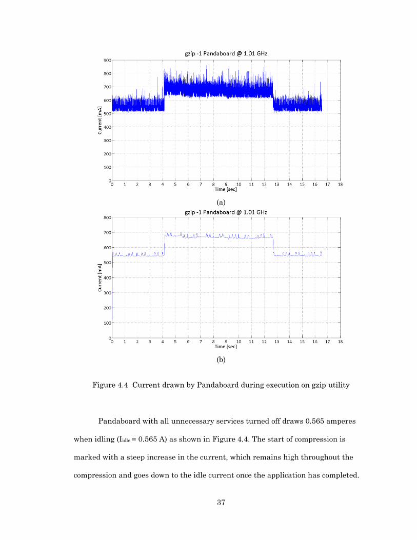
37

(a)

(b)

Figure 4.4 Current drawn by Pandaboard during execution on gzip utility

Pandaboard with all unnecessary services turned off draws 0.565 amperes

when idling (Iidle = 0.565 A) as shown in Figure 4.4. The start of compression is

marked with a steep increase in the current, which remains high throughout the

compression and goes down to the idle current once the application has completed.

38

The number of samples during the execution of a compression utility is n = T.C*SF,

where T.C is the compression time for a given file and SF is the sampling frequency.

The total energy consumed (ET.C) is calculated as follows:

tVICETn

j

jPLATFORMj 1

,. (5)

where t=1/SF, and VPLATFORM,J = VSUPPLY – IJ*R. Note that the calculation

can be simplified by assuming VPLATFORM to be constant because the voltage drop

over the shunt resistor is negligible. In addition to ET.C, the energy overhead of the

compression task, ET.C(0), is calculated alone which excludes the energy needed to

run the platform when idle. This energy overhead is calculated as:

CTVICETCET idlePLARTFORMidle ..)0(. , (6)

where VPLATFORM,idle = VSUPPLY – Iidle*R. Similarly, the total energy and the

overhead energy for decompression tasks are calculated using the decompression

time T.D instead of the compression time T.C. Once the energy overheads ET.C(0)

and ET.D(0), are determined, total energies ET.C(Iidle) and ET.D(Iidle) as a function of

the idle current using Equation (6) can be found and thus decoupling our findings

from the system under test.

4.4.2 Workstation

A typical example of running likwid-powermeter on the workstation is shown

in Figure 4.5. The first line creates a script file cmd.sh that performs a local com-

pression task using gzip with -1. To get energy estimates, the likwid-powertool is

run with the script file as a parameter. The likwid-powertool reports the conditions

and the energy estimates (from line 03 to line 12). It shows the current clock fre-

quency, the processor core id (CoreID 0) on which the task is run, the execution time,

39

and the energy consumed in Joules for the entire task (306.596 Joules) and the av-

erage power consumption (21.6 Watts).

01.~$ echo "gzip -fc -1 /dev/shm/input/enwik9.xml > /dev/null" >

cmd.sh

02.~$ likwid-powermeter ./cmd.sh

03.-------------------------------------------------------------

04.CPU name: Intel Core SandyBridge processor

05.CPU clock: 3.39 GHz

06.-------------------------------------------------------------

07.Measure on CoreId 0

08../cmd.sh

09.Runtime: 14.1936 s

10.Domain: PKG

11.Energy consumed: 306.596 Joules

12.Power consumed: 21.6011 Watts

Figure 4.5 likwid-powermeter gzip -1 example

To conduct a systematic and an autonomous way of running tasks, a bash

script is created which rewrite cmd.sh file, executes likwid-powermeter and parses

output of likwid-powermeter for energy and time for each compression and decom-

pression task repeatedly. The output of bash script produces two formatted text files,

one with energy values and another with time of execution values for compression or

decompression tasks.

4.5 Experiments

To evaluate compression and decompression tasks, three typical usage sce-

narios are considered as shown in Figure 4.7. This subsection describes the Local,

Wired and Wireless experiments performed on selected systems under test, followed

40

by description of frequency scaling (Section 4.5.1) and idle currents (Section 4.5.2)

and commands (Section 4.5.3).

The first experiment (Local) involves measuring the time and energy of com-

pression and decompression tasks performed locally on the system under test. To

eliminate latencies and energy overheads caused by reading and writing files from

the file system on the SD memory card (for Pandaboard and Raspberry Pi) or the

ATA disk (the workstation), the input files for the compression and decompression

tasks are read from the tmpfs, a temporary Linux file system stored in main

memory. The output of compression and decompression tasks is re-directed into the

Linux null device (/dev/null) – a special “file” that discards all data written to it by

calling write_null function that only increments the count with each incoming bit

(Figure 4.6).

static ssize_t write_null(struct file *file, const char __user

*buf, size_t count, loff_t *ppos)

{

return count;

}

Figure 4.6 write_null in Linux kernel source code for /dev/null

The second and third experiments (Wired and Wireless) involve measuring

the time and energy of compression and decompression tasks performed on the sys-

tem under test while communicating with a remote server. For the compression

tasks, the raw input file (UF) is read from the local tmpfs, compressed on the plat-

form, and streamed to the remote server over a secure channel. The output files are

41

redirected to the null device of the remote server. For the decompression tasks, the

compressed files (CF) are retrieved from the temporary file system of the remote

server through a secure channel and decompressed on system under test. The output

files are redirected to the null device of system under test. The communication be-

tween input, compression/decompression, and output operations is carried out

through Linux pipes. The execution times include file transfer latencies as well as

compression and decompression times. Similarly, the energies are measured for

completing the entire tasks. These two scenarios correspond to typical file-transfer

tasks on selected platforms: compressing and uploading files to a remote server, and

downloading files from a remote server and decompressing them. In addition to the

transfers that involve compression and decompression operations, the time and en-

ergy needed to upload and download the raw input file over a secure communication

channel were evaluated.

42

Figure 4.7 Experimental data flow

In the Wired experiment, system under test is connected to a local router us-

ing its Ethernet port. The remote server is also connected to the local router where

no other nodes participate in any communication. In the Wireless experiment, sys-

tem under test (Pandaboard) uses its wireless LAN interface (802.11n) to connect to

the local router and through it to the remote server. The remote server for Panda-

board and Raspberry Pi evaluation was the same computer used for evaluation of

the workstation system in this thesis, while remote server for the workstation eval-

uation was a similar workstation running Fedora distribution. The local router is a

Linksys E900 Wireless N-300 with four 10/100 Ethernet ports.

Additionally, whereas Secure Shell (SSH) adds the extra task of data encryp-

tion/decryption, it reflects current practice and better represents realistic upload and

download settings. Doing additional experiments to quantify the impact of the crypto

operations in SSH on the transfer times and the energy consumed revealed that

/dev/null

/dev/null/tmpfsUF

Compression

Decompression

CF

Pandaboard

ssh (wireless, wired)


RemoteServer

UF/tmpfs

CF

/dev/null

/dev/null/tmpfsUF

Compression

Decompression

CF

PandaboardUF

/tmpfsCF

ssh (wireless, wired) /dev/null

/tmpfsUF


UF

43

their impact is not significant when compared to the netcat and wget utilities that

do not use secure communication.

4.5.1 Frequency Scaling

To scale frequency in the mobile platforms or the workstation platform,

cpufreq-utils from linux-tools is used in this thesis. This package provides two utili-

ties, cpufreq-info and cpufreq-set. The cpufreq-info provides detailed information on

the current state of the processor as shown in Figure 4.8. The cpufreq-set allows

changing of the governor, or a policy rule for changing frequencies, maximum, min-

imum and current frequency steps.

cpufrequtils 007: cpufreq-info (C) Dominik Brodowski 2004-2009

Report errors and bugs to [email protected], please.

analyzing CPU 0:

driver: acpi-cpufreq

CPUs which run at the same hardware frequency: 0 1 2 3 4 5 6

7

CPUs which need to have their frequency coordinated by soft-

ware: 0

maximum transition latency: 10.0 us.

hardware limits: 1.60 GHz - 3.40 GHz

available frequency steps: 3.40 GHz, 3.40 GHz, 3.20 GHz, 3.00

GHz, 2.80 GHz, 2.60 GHz, 2.40 GHz, 2.20 GHz, 2.00 GHz, 1.80

GHz, 1.60 GHz

available cpufreq governors: conservative, ondemand, us-

erspace, powersave, performance

current policy: frequency should be within 1.60 GHz and 3.40

GHz.

The governor "ondemand" may decide which

speed to use

within this range.

current CPU frequency is 1.60 GHz.

cpufreq stats: 3.40 GHz:0.09%, 3.40 GHz:0.00%, 3.20

GHz:0.00%, 3.00 GHz:0.00%, 2.80 GHz:0.00%, 2.60 GHz:0.00%, 2.40

GHz:0.00%, 2.20 GHz:0.00%, 2.00 GHz:0.00%, 1.80 GHz:0.05%, 1.60

GHz:99.85% (18646)

Figure 4.8 cpufreq-info output

44

4.5.2 Idle Currents

The isolated tests are ensured by disabling any unnecessary tasks or process-

es prior to conducting any experimental runs on both mobile platforms. This in-

cludes disconnecting unused hardware (leaving only serial and power cable connect-

ed), turning off GUI interface (leaving only terminal interface), and turning off net-

work managers when no network is used.

For the Local experiment, Pandaboard has idle current of 0.51, 0.52, 0.54 and

0.55 mA for frequencies set to 300MHz, 600MHz, 900MHz and 1.01GHz respective-

ly. For the Wired experiment, Pandaboard has idle current of 0.56, 0.57, 0.59 and

0.62mA for frequencies set to 300MHz, 600MHz, 900MHz and 1.01GHz respectively.

For the Wireless experiment, Pandaboard has ide current of 0.52, 0.53, 0.54, 0.56mA

for frequencies set to 300MHz, 600MHz, 900MHz and 1.01GHz respectively. For

Raspberry Pi, idle currents for the Local and Wired tests are 0.36 and 0.42mA re-

spectively for 700MHz frequency. Table 4.3 summaries all idle currents presented in

this section.

Table 4.3 Idle Currents for Pandaboard and Raspberry Pi

Freq. Local (mA) Wired (mA) Wireless (mA) Notes

300MHz 0.51 0.56 0.52 Pandaboard 300MHz



1.01GHz 0.55 0.62 0.56 Pandaboard 1.01GHz

700MHz 0.36 0.42 - Raspberry Pi 700MHz

45

4.5.3 Commands

To perform the evaluation of compression and decompression tasks on three

experiments, several commands had to be generated. To perform time measurement

of each running task, a time utility in Linux was using together with the compres-

sion or decompression command. To perform network communication, a SSH is used

together with Linux pipes.

For the Local experiment, commands are shown in Figure 4.9 using an ex-

ample with totalInput.tar dataset. Options –f and –c and -1 represent the force of

compression or decompression, redirection of output and the selected compression

level. For decompression, option for selecting compression levels is not necessary.

Files p1_ctime_tar.txt and p2_ctime_tar.txt keep the output of the time command for

each execution.

Compression:

(time gzip –fc1 /dev/shm/input/totalInput.tar > /dev/null) 2>>

/dev/shm/p1_ctime_tar.txt

Decompression:

(time gunzip –fc /dev/shm/gzip.cfd/totalInput.1.tar.gz >

/dev/null) 2>> /dev/shm/p1_ctime_tar.txt

Figure 4.9 Commands for the Local experiment

For the Wired and Wireless experiment, commands are shown in Figure 4.10.

In addition to what was done for the Local commands, SSH and cat utilities are used

together with Linux pipes to complete network transfers. Additionally, commands

for raw transfer had to be generated for upload and download, to generate evalua-

46

tion data for the network transfer which is compared to compression and decompres-

sion tasks.

Compression: (time gzip -fc1 /dev/shm/input/totalInput.tar | ssh ar-

mend@xeon-server "cat > /dev/null")

2>>/run/shm/p2_ctime_tar.txt

Decompression (time ssh armend@xeon-server "cat

/dev/shm/gzip.cfd/totalInput.1.tar.gz" |gunzip -fc > /dev/null)

2>>/run/shm/p2_dtime_tar.txt

Upload (time cat /run/shm/input/totalInput.tar | ssh armend@xeon-

server "cat

> /dev/null") 2>>/run/shm/p2_UC_ctime_tar.txt

Download (time ssh armend@xeon-server "cat

/dev/shm/input/totalInput.tar" | cat > /dev/null)

2>>/run/shm/p2_UC_dtime_tar.tx

Figure 4.10 Commands for the Wired and Wireless experiments

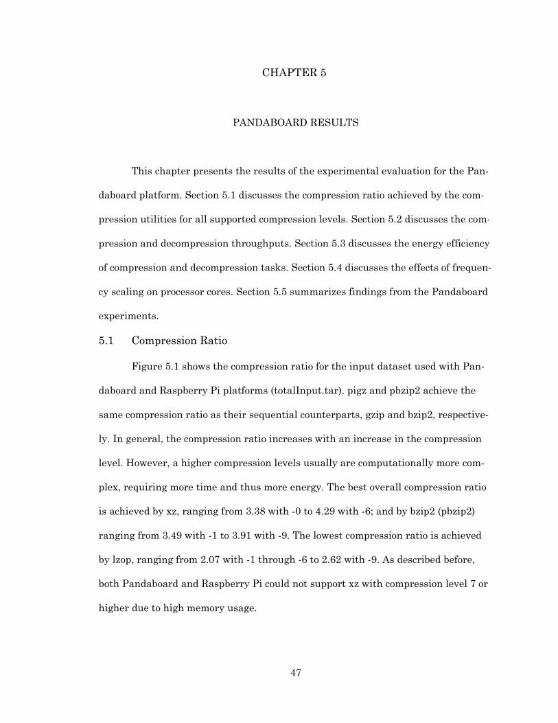
47

CHAPTER 5

PANDABOARD RESULTS

This chapter presents the results of the experimental evaluation for the Pan-

daboard platform. Section 5.1 discusses the compression ratio achieved by the com-

pression utilities for all supported compression levels. Section 5.2 discusses the com-

pression and decompression throughputs. Section 5.3 discusses the energy efficiency

of compression and decompression tasks. Section 5.4 discusses the effects of frequen-

cy scaling on processor cores. Section 5.5 summarizes findings from the Pandaboard

experiments.

5.1 Compression Ratio

Figure 5.1 shows the compression ratio for the input dataset used with Pan-

daboard and Raspberry Pi platforms (totalInput.tar). pigz and pbzip2 achieve the

same compression ratio as their sequential counterparts, gzip and bzip2, respective-

ly. In general, the compression ratio increases with an increase in the compression

level. However, a higher compression levels usually are computationally more com-

plex, requiring more time and thus more energy. The best overall compression ratio

is achieved by xz, ranging from 3.38 with -0 to 4.29 with -6; and by bzip2 (pbzip2)

ranging from 3.49 with -1 to 3.91 with -9. The lowest compression ratio is achieved

by lzop, ranging from 2.07 with -1 through -6 to 2.62 with -9. As described before,

both Pandaboard and Raspberry Pi could not support xz with compression level 7 or

higher due to high memory usage.

48

Figure 5.1 Pandaboard and Raspberry Pi: Compression Ration (totalInput.tar)

5.2 Compression and Decompression Throughputs

5.2.1 Local

Figure 5.2 shows the overall compression and decompression throughputs for

the Local experiment expressed in MB/sec. The compression throughput varies wide-

ly across different compression utilities as well as across different compression levels

of a single compression utility. For all compression utilities, the higher compression

levels result in lower throughputs. By far the highest compression throughput of ~25

MB/sec is achieved by lzop -1 to -6. However, throughput of lzop drops dramatically

to 1.37, 0.7, and 0.6 MB/sec for the highest compression levels (-7, -8 and -9 respec-

tively). The second highest compression throughput from 13.2 to 2 MB/sec is

achieved by pigz. It fully utilizes two processor cores to achieve close to double the

compression throughput relative to gzip (from 7.4 to 1 MB/sec). In contrast, xz and

bzip2 achieve significantly lower compression throughputs (e.g., from 1.6 to 1.1

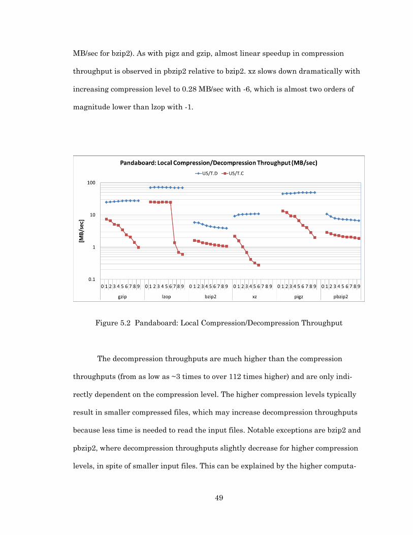
49

MB/sec for bzip2). As with pigz and gzip, almost linear speedup in compression

throughput is observed in pbzip2 relative to bzip2. xz slows down dramatically with

increasing compression level to 0.28 MB/sec with -6, which is almost two orders of

magnitude lower than lzop with -1.

Figure 5.2 Pandaboard: Local Compression/Decompression Throughput

The decompression throughputs are much higher than the compression

throughputs (from as low as ~3 times to over 112 times higher) and are only indi-

rectly dependent on the compression level. The higher compression levels typically

result in smaller compressed files, which may increase decompression throughputs

because less time is needed to read the input files. Notable exceptions are bzip2 and

pbzip2, where decompression throughputs slightly decrease for higher compression

levels, in spite of smaller input files. This can be explained by the higher computa-

50

tional complexity of bzip2’s decompression when input files are generated using

higher compression levels. The highest decompression throughput of 71.9 MB/sec is

achieved by lzop, followed by pigz (45.3 to 49.6 MB/sec) and gzip (24.7 to 27.5

MB/sec). xz achieves ~10 MB/sec, whereas pbzip2 ranges from 10.7 to 6.6 MB/sec

and bzip2 from 5.8 to 3.8 MB/sec (both having lower decompression throughputs for

higher compression levels). It should be noted that pigz and pbzip2 offer improve-

ments in decompression throughputs over their sequential counterparts. Although

decompression itself in pigz is not parallelized (it is single threaded), three other

threads are created for reading, writing, and checking calculations that speed up de-

compression [19]. pbzip2’s implementation includes parallelized decompression, thus

fully benefiting from the dual-core processor in the OMAP4430 in Pandaboard.

5.2.2 Wired

Figure 5.3 shows the compression and decompression throughputs in the

Wired experiment. The dashed lines represent the measured effective network

throughput when the uncompressed input file is uploaded to the remote server

(US/T.UUP = 5.95 MB/sec) and downloaded from the remote server (US/T.UDW =

8.84 MB/sec).

The compression throughput is limited by the effective network throughput

and therefore it is always below the CR*(US/T.UUP). For example, lzop -1 (through -

6) plateaus at 11 MB/sec, which is below 2.07*5.95 = 12.3 MB/sec (the compression

ratio for lzop -1 is 2.07). The effective compression throughput in this case is thus

significantly below the 25 MB/sec measured in the Local experiment. However, for

lzop with -7, -8, and -9, where the original compression throughput is lower than the

upload network throughput (5.95 MB/sec), the compression throughputs remain un-

51

changed relative to those measured in the Local experiment. Similar observations

can be made about the other compression utilities. For gzip and pigz with -1, the

compression throughputs are 6 and 8.3 MB/sec, respectively, well below the maxi-

mum achievable 15.8 MB/sec (2.65*5.95, where 2.65 is the compression ratio for gzip

and pigz with -1). pigz with low compression levels offers only slightly higher com-

pression throughput relative to gzip, but it almost doubles the throughput with high

compression levels (e.g., 1.84 MB/sec vs. 0.95 MB/sec with -9). In contrast, pbzip2

consistently offers a higher compression throughput relative to bzip2 because they

both have a compression throughput that is below the effective network upload

throughput. When compared to the throughput for uploading the uncompressed da-

taset, only lzop with -1 to -6, gzip with -1, and pigz with -1 to -4 provide an increased

effective network throughput, whereas the other combinations do not appear to be

beneficial (i.e., it takes more time to compress and upload an input file than to just

upload the raw input file).

52

Figure 5.3 Pandaboard: Wired Compression/Decompression Throughput

The decompression throughputs are also limited by the effective network

throughput, resulting in lower effective decompression throughputs, which are below

CR*(US/T.UDW). For example, lzop with -9 achieves a decompression throughput of

~20.8 MB/sec, which is very close to the maximum achievable (2.62*8.84 = 23.2

MB/sec) but far below the 70 MB/sec measured in the Local experiment. gzip with -9

achieves ~22.6 MB/sec and pigz with -9 achieves ~23.5 MB/sec. They outperform lzop

because they provide higher compression ratios – their achievable maximum decom-

pression throughput is below 2.99*8.84 = 26.4 MB/sec. These three utilities effective-

ly increase the available network throughput (their throughputs are above the

US/T.UDW line) and decrease the download time relative to the time needed to

download uncompressed files from the remote server. pbzip2 and bzip2 suffer from

minor decreases in their effective decompression throughput relative to the Local

experiment (due to the network latency) because their original decompression

53

throughput falls below the available network throughput for downloads (8.84

MB/sec). xz is on the boundary with its effective throughput ranging from 8.6 to 9.9

MB/sec (down from 9.1 to 10.8 MB/sec in the Local experiment).

5.2.3 Wireless

Figure 5.4 shows the compression and decompression throughputs for the

Wireless experiment. The dashed lines represent the measured effective upload and

download throughput when transferring the uncompressed file wirelessly, where

US/T.UUP = 1.64 MB/sec (13.12 Mbits/sec) and US/T.UDW = 1.52 MB/sec (12.16

Mbits/sec), respectively. Similar to the prior experiments, the effective compression

throughput is limited by the network upload throughput and is always below

CR*(US/T.UUP). In the Wireless experiment, compression effectively increases the

upload throughput for gzip with -1 to -7, lzop with -1 to -6, xz with -0, pigz with -1 to

-9, and pbzip2 with -1 to -9, whereas bzip2 falls below 1.52 MB/sec. The lower effec-

tive network throughputs enable more compression configurations to be beneficial.

Compression with lower compression levels is still preferred to higher levels. The

highest compression throughput of ~5.1 MB/sec is achieved by pigz with -1. It out-

performs gzip -1 (4.1 MB/sec) and lzop -1 (3.2 MB/sec).

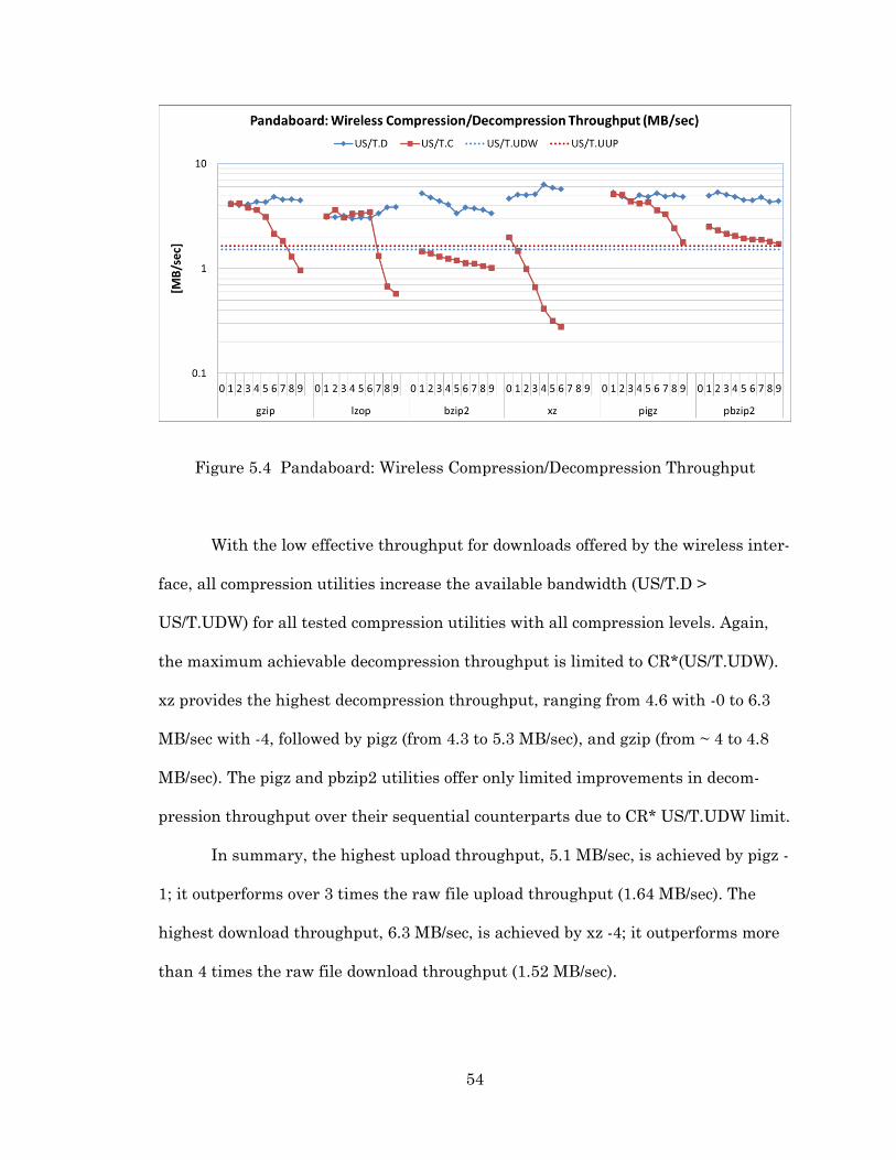
54

Figure 5.4 Pandaboard: Wireless Compression/Decompression Throughput

With the low effective throughput for downloads offered by the wireless inter-

face, all compression utilities increase the available bandwidth (US/T.D >

US/T.UDW) for all tested compression utilities with all compression levels. Again,

the maximum achievable decompression throughput is limited to CR*(US/T.UDW).

xz provides the highest decompression throughput, ranging from 4.6 with -0 to 6.3

MB/sec with -4, followed by pigz (from 4.3 to 5.3 MB/sec), and gzip (from ~ 4 to 4.8

MB/sec). The pigz and pbzip2 utilities offer only limited improvements in decom-

pression throughput over their sequential counterparts due to CR* US/T.UDW limit.

In summary, the highest upload throughput, 5.1 MB/sec, is achieved by pigz -

1; it outperforms over 3 times the raw file upload throughput (1.64 MB/sec). The

highest download throughput, 6.3 MB/sec, is achieved by xz -4; it outperforms more

than 4 times the raw file download throughput (1.52 MB/sec).

55

5.3 Energy Efficiency

5.3.1 Local

Figure 5.5 and Figure 5.6 show the energy efficiency for the compression and

decompression tasks for the Local experiment reported in MB/J (US/ET.C and

US/ET.D) and in MB/J (|US-CS|/ET.C and |US-CS|/ET.D) as a function of the

idle current Iidle (Iidle ={0, 0.25, 0.5, 0.75} A). In contrast to MB/J metric, MB/J is a

function of the amount of data removed by compression |US-CS|. Thus, this metric

captures the strength of the compression utilities and compression level. To under-

stand this better, |US-CS|/ET.C and |US-CS|/ET.D can be rewritten as (1-

1/CR)*US/ET.C and (1-1/CR)*US/ET.D. The variable (1-1/CR) increases with in-

crease in compression, thus all data points across both datasets for compression and

decompression should be scaled by individual amount that depends on compression

ratio. Knowing the lowest and the highest compression ratio in totalInput.tar da-

taset from Section 5.1, (1-1/CR) ranges from 0.52 to 0.76.

The energy efficiency of the compression tasks varies widely for different

utilities and for different compression levels within each utility (often by more than

an order of magnitude), as shown in Figure 5.5. The most energy efficient compres-

sion utility by far is lzop with compression levels -1 to -6 regardless of the idle cur-

rent; it achieves ~54 MB/J (MB/joule) for Iidle = 0 A, ~14.5 MB/J for Iidle = 0.25 A, and

8.5 MB/J for Iidle = 0.5 A. Distant second and third are gzip and pigz with -1 achiev-

ing ~14 MB/J and ~11 MB/J for Iidle = 0. Following the trends in compression

throughputs, higher compression levels for gzip, pigz, and lzop result in a dramatic

decrease in energy efficiency (e.g., down to 1.5 MB/J for lzop with -9). pigz and

pbizp2 are more energy efficient than their sequential counterparts when Iidle ≠ 0 A

56

because they reduce the compression time. However, if we consider only the energy

efficiency when Iidle = 0 A (US/ET.C(0)), the parallel implementations are slightly

less energy efficient. pbzip2 and bzip2 exhibit low energy efficiencies as does xz,

which is the least attractive choice with high compression levels. The alternative en-

ergy efficiency expressed in MB/J follows similar trends as the regular energy effi-

ciency.

57

(a)

(b)

Figure 5.5 Pandaboard: Local Energy Efficiency for Compression

The energy efficiency of the decompression tasks varies widely for different

utilities as shown in Figure 5.6. The energy efficiency is relatively stable for individ-

ual utilities – it increases slightly for higher compression levels for all utilities ex-

cept bzip2 and pbizp2. Thus, US/ET.D(0) is ~136 MB/J for lzop, ~50 MB/J for gzip,

58

~55 for pigz, and just below ~10 MB/J for bzip2/pbzip2. lzop emerges as the most en-

ergy-efficient choice in spite of its lower compression ratio. These observation hold

for the alternative definition of energy efficiency defined as (US-CS)/ET.D.

(a)

(b)

Figure 5.6 Pandaboard: Local Energy Efficiency for Decompression

59

5.3.2 Wired

Figure 5.7 and Figure 5.8 show the energy efficiency for compression and de-

compression tasks for the Wired experiment reported in MB/J and in MB/J as a

function of the idle current. In addition, Figure 5.7(a) and Figure 5.8(a) show the en-

ergy efficiency for uncompressed upload (US/ET.UUP) and uncompressed download

(US/ET.UDW) as a function of the idle current. This way, one can easily identify

cases when compression and decompression transfers offer higher energy efficiency

than raw uploads (US/ET.C(Iidle) > US/UUP(Iidle)) and raw downloads (US/ET.D(Iidle)

> US/ET.UDW(Iidle)). With MB/J metric, on other hand, energy efficiency for raw

network transfer cannot be reported.

The energy efficiency for compression is reported in Figure 5.7. When Iidle = 0,

gzip, pigz, and lzop with -1 to -7 and xz with -1 to -2 provide higher energy efficiency

than the raw network upload. However, only lzop with -1 to -6, gzip -1 to -4, and pigz

-1 to -5 provide higher energy efficiency for all considered idle currents. The most

energy efficient utility is again lzop with -1 to -6 achieving ~12.5 MB/J when Iidle = 0,

~5MB/J when Iidle = 0.25 A, and ~3.25 MB/J when Iidle = 0.5 A. bzip2, pbizp2, and xz

exhibit rather low energy efficiency for compression. These observations hold when

the alternative energy efficiency metric is considered.

60

(a)

(b)

Figure 5.7 Pandaboard: Wired Energy Efficiency for Compression

The energy efficiency of the decompression tasks using gzip, lzop, and pigz

exceeds the energy efficiency of the uncompressed download for all considered idle

currents, whereas xz is only slightly beneficial, and bzip2 and pbzip2 are less energy

efficient (Figure 5.8). The energy efficiency slightly increases for higher compression

61

levels (except for bzip2/pbzip2), achieving ~23.7 MB/J for lzop, ~ 21 MB/J for pigz,

and ~19 MB/J for gzip when Iidle = 0 A. pigz emerges as the most energy-efficient

utility, slightly outperforming gzip and lzop when Iidle = {0.25, 0.5, 0.75} A.

(a)

(b)

Figure 5.8 Pandaboard: Wired Energy Efficiency for Decompression

62

5.3.3 Wireless

Figure 5.9 and Figure 5.10 show the energy efficiency for the compression

and decompression tasks for the Wireless experiment reported in MB/J and in

MB/J as a function of the idle current. Similar to the previous experiment, the

graphs also display the energy efficiency for uncompressed upload (US/ET.UUP) and

uncompressed download (US/ET.UDW) as a function of the idle current.

The energy efficiency for compression is reported in Figure 5.9. The relatively

low network throughput for upload results in all utilities having higher energy effi-

ciency than the raw upload when Iidle = 0 A (i.e., US/ET.C(0) > US/ET.UUP(0)) for all

utilities except xz -5 and -6. pigz -1 is the most energy efficient with 2.5 MB/J, fol-

lowed closely by gzip -1 and lzop -1. pigz -1 remains the most energy-efficient com-

pression utility when Iidle = {0.25, 0.5, 0.75} A. For the MB/J metric, the distribution

of energy efficiency is the same for all utilities except lzop. lzop is lowered by a small

degree in comparison with pigz and gzip.

63

(a)

(b)

Figure 5.9 Pandaboard: Wireless Energy Efficiency for Compression

All decompression alternatives offer a total energy efficiency that exceeds the

total energy efficiency of uncompressed download from the remote server,

US/ET.UDW(0), which is 1.16 MB/J (Figure 5.10). Downloading files that were com-

pressed with higher compression levels increase the energy efficiency except for

64

bzip2 and pbzip2. The total energy efficiency when Iidle = 0 A, US/ET.D(0), is ~3.6 -

4.3 MB/J for gzip, 2.9 - 3.7 MB/J for lzop, 4 - 4.8 MB/J for pigz, 2.9 - 3.1 MB/J for

pbzip2, and 3.6 - 4.6 MB/J for xz. pigz and xz emerge as the most energy-efficient

utilities when Iidle = {0.25, 0.5, 0.75} A. xz benefits from providing a superior com-

pression ratio in conditions when communication energy dominates the overall ener-

gy costs.

65

(a)

(b)

Figure 5.10 Pandaboard: Wireless Energy Efficiency for Decompression

5.4 Frequency scaling

The frequency scaling for the Pandaboard platform covers frequency steps of

300MHz, 600MHz, 800MHz and 1.01GHz (with highest frequency used to describe

the results from Section 5.2 and Section 5.3). To evaluate the effects of frequency

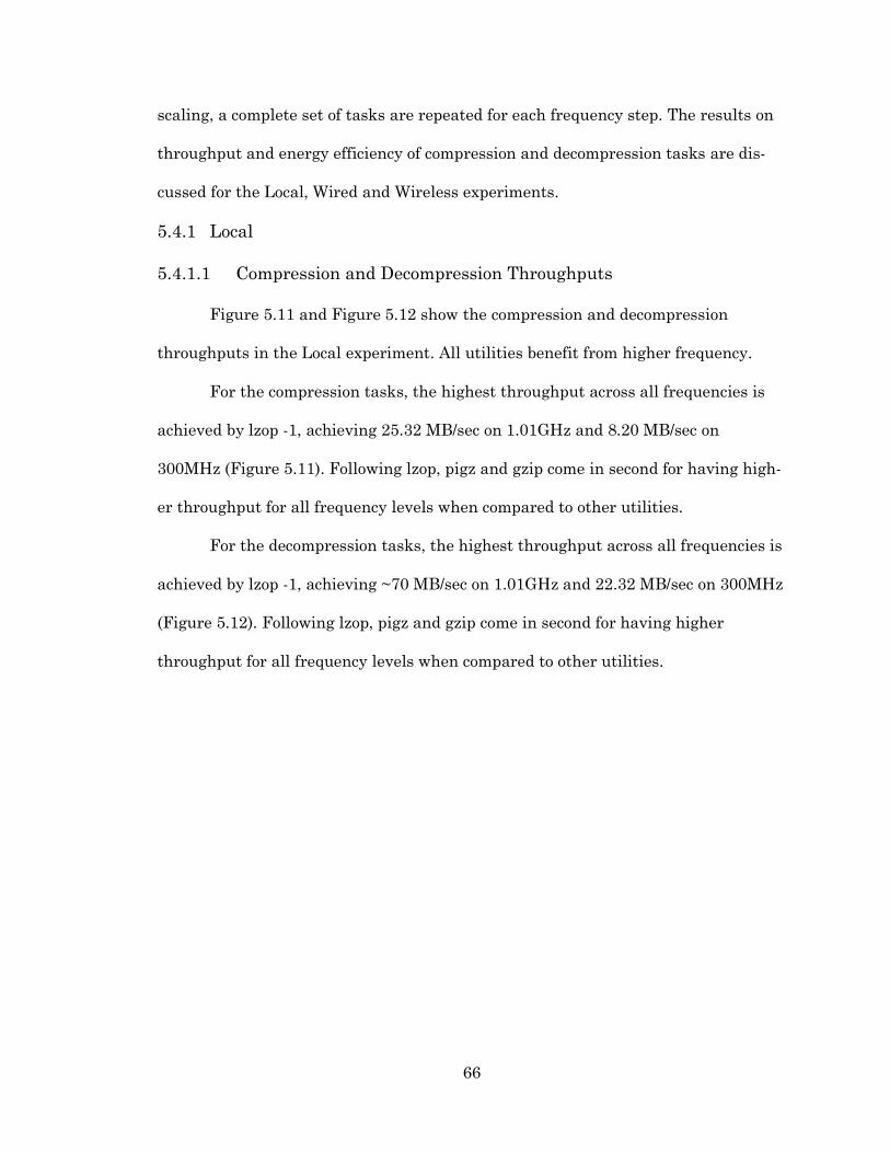
66

scaling, a complete set of tasks are repeated for each frequency step. The results on

throughput and energy efficiency of compression and decompression tasks are dis-

cussed for the Local, Wired and Wireless experiments.

5.4.1 Local

5.4.1.1 Compression and Decompression Throughputs

Figure 5.11 and Figure 5.12 show the compression and decompression

throughputs in the Local experiment. All utilities benefit from higher frequency.

For the compression tasks, the highest throughput across all frequencies is

achieved by lzop -1, achieving 25.32 MB/sec on 1.01GHz and 8.20 MB/sec on

300MHz (Figure 5.11). Following lzop, pigz and gzip come in second for having high-

er throughput for all frequency levels when compared to other utilities.

For the decompression tasks, the highest throughput across all frequencies is

achieved by lzop -1, achieving ~70 MB/sec on 1.01GHz and 22.32 MB/sec on 300MHz

(Figure 5.12). Following lzop, pigz and gzip come in second for having higher

throughput for all frequency levels when compared to other utilities.

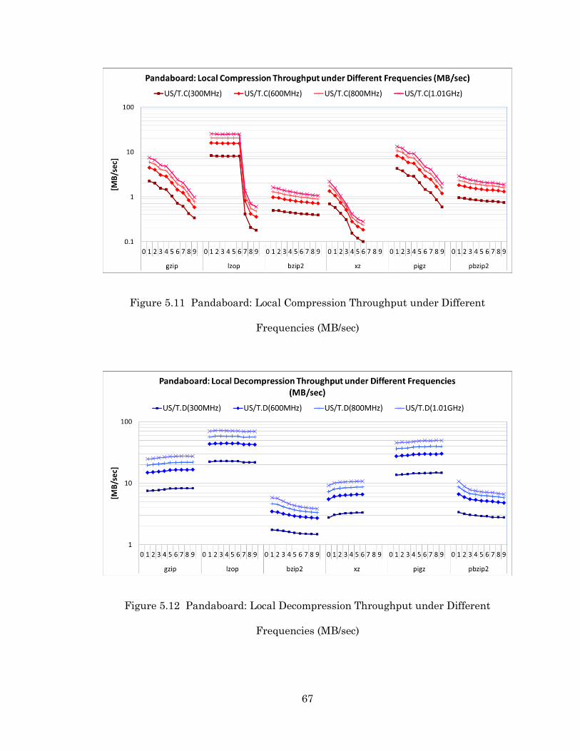
67

Figure 5.11 Pandaboard: Local Compression Throughput under Different

Frequencies (MB/sec)

Figure 5.12 Pandaboard: Local Decompression Throughput under Different

Frequencies (MB/sec)

68

Figure 5.13 shows comparison between throughput ratios and frequency rati-

os for the compression and decompression tasks in the Local experiment. The

throughput ratio is derived by dividing the throughput achieved for highest frequen-

cy (1.01 GHz) by the throughput achieved for other frequencies (300MHz, 600MHz

or 800MHz). This ratio is compared to the frequency ratio derived by dividing the

highest frequency by the corresponding frequency (300MHz, 600MHz or 800MHz).

The utilities such as gzip, lzop and pigz have almost identical throughput ratios as

their corresponding frequency ratios, indicating linear relationship between fre-

quency scaling and throughput change. Similar observation can be made for xz dur-

ing decompression. The higher compression levels of bzip2 and pbzip2 have lower

throughput ratios when compared with their frequencies ratios, indicating non-

linear throughput change with frequency scaling on higher compression levels. The

same observation can be made for higher compression levels of xz during compres-

sion.

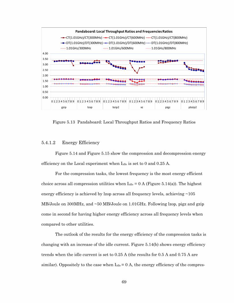
69

Figure 5.13 Pandaboard: Local Throughput Ratios and Frequency Ratios

5.4.1.2 Energy Efficiency

Figure 5.14 and Figure 5.15 show the compression and decompression energy

efficiency on the Local experiment when Iidle is set to 0 and 0.25 A.

For the compression tasks, the lowest frequency is the most energy efficient

choice across all compression utilities when Iidle = 0 A (Figure 5.14(a)). The highest

energy efficiency is achieved by lzop across all frequency levels, achieving ~105

MB/Joule on 300MHz, and ~50 MB/Joule on 1.01GHz. Following lzop, pigz and gzip

come in second for having higher energy efficiency across all frequency levels when

compared to other utilities.

The outlook of the results for the energy efficiency of the compression tasks is

changing with an increase of the idle current. Figure 5.14(b) shows energy efficiency

trends when the idle current is set to 0.25 A (the results for 0.5 A and 0.75 A are

similar). Oppositely to the case when Iidle = 0 A, the energy efficiency of the compres-

70

sion utilities increase for higher frequencies, achieving the best energy efficiency at

the highest frequency of 1.01 GHz.

(a)

(b)

Figure 5.14 Pandaboard: Local Energy Efficiency for Compression under Different

Frequencies

71

For the decompression tasks, the lowest frequency is most energy efficient

choice across all decompression utilities when Iidle = 0 A (Figure 5.15(a)). The highest

energy efficiency is achieved by lzop across all frequency levels, achieving ~260

MB/Joule on 300MHz, and ~137 MB/Joule on 1.01GHz. Following lzop, pigz and gzip

come in second for having higher energy efficiency across all the frequency levels

when compared to other utilities.

The outlook of the results for energy efficiency of the decompression tasks is

changing with an increase of the idle current. Figure 5.15(b) shows energy efficiency

trends for the decompression tasks when the idle current is set to 0.25 A. Oppositely

to the case when Iidle = 0 A, the energy efficiency of the decompression utilities in-

crease for the higher frequencies, achieving the best energy efficiency at the highest

frequency of 1.01 GHz.

72

(a)

(b)

Figure 5.15 Pandaboard: Local Energy Efficiency for Decompression under Different

Frequencies

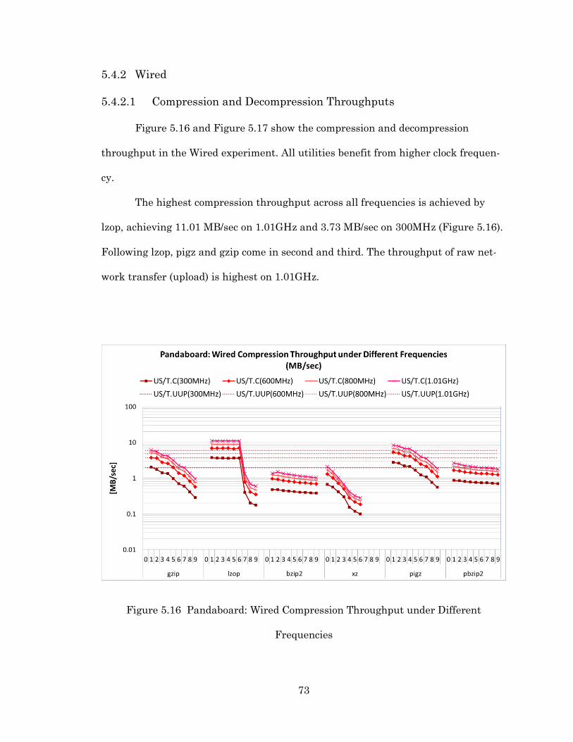
73

5.4.2 Wired



throughput in the Wired experiment. All utilities benefit from higher clock frequen-

cy.

The highest compression throughput across all frequencies is achieved by

lzop, achieving 11.01 MB/sec on 1.01GHz and 3.73 MB/sec on 300MHz (Figure 5.16).

Following lzop, pigz and gzip come in second and third. The throughput of raw net-

work transfer (upload) is highest on 1.01GHz.

Figure 5.16 Pandaboard: Wired Compression Throughput under Different

Frequencies

74

The highest decompression throughput across all frequencies is achieved by

pigz -9, achieving ~23.4 MB/sec on 1.01GHz and 8.04 MB/sec on 300MHz (Figure

5.17). Following pigz, gzip and lzop come in second and third for having higher

throughput for all frequency levels when compared to other utilities (gzip -9 with

22.59 MB/sec at 1.01GHz and ~7 MB/sec on 300MHz and lzop -9 with 20.88 MB/sec

on 1.01GHz and ~7 MB/sec at 300MHz). The throughput of raw network transfer

(download) is highest on 1.01GHz.

Figure 5.17 Pandaboard: Wired Decompression Throughput under Different

Frequencies

Figure 5.18 shows a comparison between throughput ratios and frequency ra-

tios for compression and decompression on the Wired experiment. The throughput

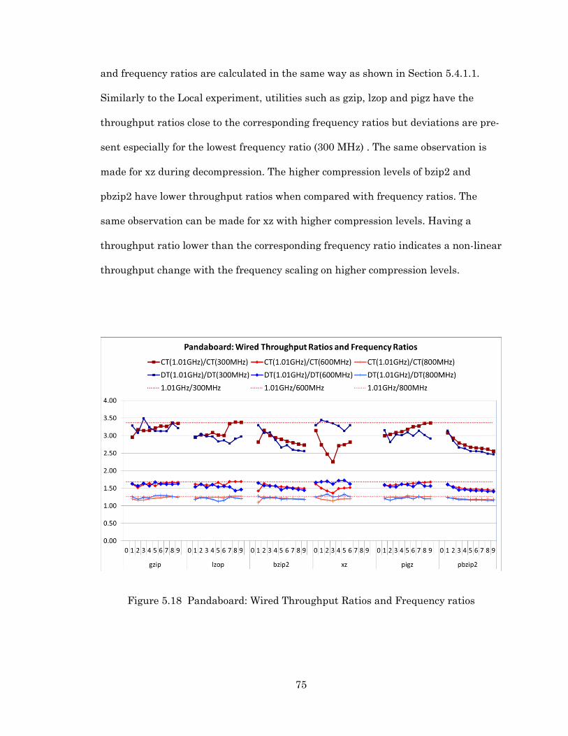
75

and frequency ratios are calculated in the same way as shown in Section 5.4.1.1.

Similarly to the Local experiment, utilities such as gzip, lzop and pigz have the

throughput ratios close to the corresponding frequency ratios but deviations are pre-

sent especially for the lowest frequency ratio (300 MHz) . The same observation is

made for xz during decompression. The higher compression levels of bzip2 and

pbzip2 have lower throughput ratios when compared with frequency ratios. The

same observation can be made for xz with higher compression levels. Having a

throughput ratio lower than the corresponding frequency ratio indicates a non-linear

throughput change with the frequency scaling on higher compression levels.

Figure 5.18 Pandaboard: Wired Throughput Ratios and Frequency ratios

76



efficiency on the Wired experiment when Iidle is set to 0 and 0.25 A, respectively.

The lowest frequency is the most energy efficient choice across all compres-

sion tasks when Iidle = 0 A (Figure 5.19(a)). The highest energy efficiency is achieved

by lzop across all frequency levels, achieving ~45 MB/Joule on 300MHz, and ~12.3

MB/Joule on 1.01GHz. Following lzop, pigz and gzip come in second and third for

having higher energy efficiency for all frequency levels when compared to other utili-

ties. The energy efficiency of the raw network upload, on other hand, is highest on

1.01GHz.

The results for energy efficiency of compression tasks change with an in-

crease of the idle current. Figure 5.19(b) shows the energy efficiency when the idle

current is set to 0.25 A. The energy efficiency of the compression tasks increase with

an increase in the clock frequency, achieving the best energy efficiency at the high-

est frequency of 1.01 GHz. The energy efficiency of raw file download follows the

same trend.

77

(a)

(b)

Figure 5.19 Pandaboard: Wired Energy Efficiency for Compression under Different

Frequencies

The lowest frequency is the most energy efficient choice across all decompres-

sion utilities when Iidle = 0 A (Figure 5.20(a)). The highest energy efficiency is

achieved by lzop across all frequency levels, achieving from ~60 to 90 MB/Joule on

78

300MHz, and ~23.6 MB/Joule on 1.01GHz. Following lzop, pigz and gzip come in

second and third for having higher energy efficiency across all frequency levels when

compared to the other utilities. The energy efficiency of the raw file download is

highest for the 300MHz clock frequency.

The energy efficiency of the decompression tasks is changing with an increase

of the idle current. Figure 5.20(b) shows energy efficiency trends for decompression

when the idle current is set to 0.25 A. The energy efficiency of the decompression

utilities increases for higher clock frequencies, achieving the best energy efficiency

at the highest frequency of 1.01 GHz. The energy efficiency of the raw file download

peaks at the highest clock frequency.

79

(a)

(b)

Figure 5.20 Pandaboard: Wired Energy Efficiency for Decompression under

Different Frequencies

80

5.4.3 Wireless



throughput in the Wireless experiment. All utilities benefit from higher clock fre-

quency.

The highest compression throughput across higher frequencies (800MHz and

1.01GHz) is achieved by pigz -1, achieving 5.1 MB/sec on 1.01 GHz (Figure 5.21).

The highest compression throughput across lower frequencies (300MHz and

600MHz) is achieved by lzop -1 to 6, achieving 2.8 MB/sec on 300MHz. The through-

put of raw network transfer (upload) is highest on 1.01GHz.

Figure 5.21 Pandaboard: Wireless Compression Throughput under Different

Frequencies

81

The highest decompression throughput across higher frequencies is achieved

by xz, achieving 6.49 MB/sec on 1.01GHz (Figure 5.22). The highest decompression

throughput on the lowest frequency is achieved by pigz, gzip and lzop. The through-

put of raw network transfer (download) is highest on 300MHz.

Figure 5.22 Pandaboard: Wireless Decompression Throughput under Different

Frequencies

Figure 5.23 shows a comparison between throughput ratios and frequency ra-

tios for compression and decompression on the Wireless experiment. Derivation of

throughput and frequency ratios follows same example made before in Section

5.4.1.1. The distribution of ratios, however, differs on the Wireless experiment from

82

those demonstrated for the Local and Wired experiments in Section 5.4.1 and Sec-

tion 5.4.2. Now, only some compression utilities and only certain compression levels

achieve throughput ratio that is equal to or very close to the corresponding frequen-

cy ratio. This is now only true for compression utilities such as gzip -5 to -9, lzop -7

to -9, pigz -6 to -9, bzip2 -1 and pbzip2 -1. For compression, greatest benefit from

downward frequency scaling can be seen in lzop -1 to -6 for 1.01 GHz to 300 MHz

case, with T.C(1.01GHz)/T.C(300MHz) being ~1.2 while 1.01GHz/600MHz ratio is

3.37. For decompression, the downward frequency scaling is beneficial to almost all

utilities, with throughput ratios of all utilities, except of bzip2, being much lower

than the corresponding frequency ratio.

Figure 5.23 Pandaboard: Wireless Throughput Ratios and Frequency Ratios

83



efficiency on the Wireless experiment when Iidle is set to 0 and 0.25 A.

The lowest frequency is the most energy efficient choice across selected com-

pression utilities when Iidle = 0 A (Figure 5.24(a)). The utilities that benefit from low-

est frequency are pbzip2, bzip2 and xz. The utilities that benefit from higher fre-

quencies are pigz, gzip and lzop (with small differences between frequencies

600MHz, 800MHz and 1.01GHz). The highest energy efficiency is achieved by lower

levels of pigz, lzop -1 to -6, and lower levels of gzip across all frequency levels. The

energy efficiency of raw network energy efficiency (upload) does not change with fre-

quency scaling.

The results for energy efficiency of compression tasks change with an in-

crease of the idle current. Figure 5.24(b) shows energy the efficiency when the idle

current is set to 0.25 A. The energy efficiency of the compression tasks increase with

an increase in the clock frequency, achieving the best energy efficiency at the high-

est frequency of 1.01 GHz. The energy efficiency of raw network transfer (download)

does not change with frequency scaling.

84

(a)

(b)

Figure 5.24 Pandaboard: Wireless Energy Efficiency for Compression under


The lowest frequency is most energy efficient choice only for selected decom-

pression utilities when Iidle = 0 A (Figure 5.25(a)). The highest energy efficiency is

achieved by lzop across all frequency levels, achieving 7.34 MB/Joule on 300MHz,

85

and 4.55 MB/Joule on 1.01GHz. Following lzop, pigz and gzip come in second and

third for having higher energy efficiency across all frequency levels when compared

to other utilities. The energy efficiency of raw network energy efficiency (upload)

does not change with frequency scaling.

The energy efficiency of the decompression tasks is changing with an increase

of the idle current. Figure 5.25(b) shows energy efficiency trends for decompression

when the idle current is set to 0.25 A. Similarly to the case when Iidle = 0 A, the low-

est frequency is most energy efficient choice only for selected decompression utilities,

such as pigz, gzip and lzop. However, the difference between the energy efficiency at

the highest and the lowest frequency is much smaller. For this reason, the best

overall energy efficiency is achieved by xz at higher frequencies (600 MHz, 800 MHz,

1.01 GHz). The energy efficiency of raw file download does not change with frequen-

cy scaling.

86

(a)

(b)

Figure 5.25 Pandaboard: Wireless Energy Efficiency for Decompression under


5.5 Conclusions

The experimental results for the Pandaboard platform show that compression

is best at the lowest compression levels, and decompression is best at the highest

87

compression level (for exception of bzip2 and pbzip2) for both the throughput and

energy efficiency.

Table 5.1 summarizes the throughput results. lzop performs the best for com-

pression and decompression in the Local experiment and for compression in the

Wired experiment. The best throughput for decompression in the Wired experiment

is achieved by pigz, followed by gzip and then lzop (pigz outperforms lzop by 3.67%).

For the Wireless experiment, pigz with -1 performs the best for compression and xz

with -4 performs the best for decompression.

Table 5.1 Throughputs on Pandaboard @ 1.01GHz

Experiment Compression Raw

(UUP)

Decompression Raw

(UDW)

Best Utility

Th.C [MB/s]

Th.UUP [MB/s]

Best Utility

Th.D [MB/s]

Th.UWD [MB/s]

LOCAL lzop -1 to -6 25 lzop -1 to -9 70

WIRED lzop -1 to -6 11 5.95 pigz -6 to -9 23.5 8.84

WIRELESS pigz -1 5.1 1.64 xz -4 6.28 1.52

Table 5.2 shows the energy efficiency. lzop is the most energy-efficient for

both the Local and Wired experiment for compression and decompression. pigz, gzip

and xz outperform lzop in the Wireless experiment. For compression, pigz has the

best energy efficiency, followed by gzip and lzop. For decompression, when Iidle is 0 A,

pigz has the best energy efficiency, followed by xz, gzip, and lzop. However, when Iidle

is 0.25, 0.5 or 0.75, xz overtakes pigz in the energy efficiency. The results show that

compressed network transfers are more energy efficient that raw network transfers.

In the Wired experiment, the most energy efficient compressed upload with pigz -1

88

achieves 12.4 MB/J, which ~7.8 times more energy efficient than 1.59 MB/J achieved

with the uncompressed upload (assuming Iidle = 0 A). The most energy-efficient de-

compressed download using lzop with -9 achieves 23.5 MB/J, which is ~2.5 times

better than the uncompressed download that achieves 9.43 MB/J. In the Wireless

experiment, the most energy-efficient upload using pigz with -1 achieves 2.5 MB/J,

compared to 0.39 MB/J achieved by the uncompressed upload (> 6 times improve-

ment). Similarly, the decompressed download offers almost 4 times higher energy

efficiency than the uncompressed download.

Table 5.2 Energy Efficiency on Pandaboard @ 1.01GHz


(UUP)

Decompression Raw

(UDW)

LOCAL

Best Utility

EE.C [MB/J]

EE.UUP [MB/J]

Best Utility

EE.D [MB/J

]

EE.UDW [MB/J]

Iidle = 0 A lzop -1 to -6 55 lzop -6 to -9 137

Iidle = 0.25 A lzop -1 to -6 14.5 lzop -6 to -9 40


WIRED

Iidle = 0 A lzop -1 to -6 12.4 1.59 lzop -7 to -9 23.5 9.43

Iidle = 0.25 A lzop -1 to -6 5.1 1.19 pigz -6 to -9 10 4.04

Iidle = 0.5 A lzop -1 to -6 3.2 0.95 pigz -6 to -9 6.5 2.57

WIRELESS

Iidle = 0 A pigz -1 2.5 0.39 pigz -4 to -7 4.6 1.16

Iidle = 0.25 A pigz -1 1.5 0.30 xz -4 to -6 2.4 0.59

Iidle = 0.5 A pigz -1 1.1 0.25 xz -4 to -6 1.6 0.40

Use of parallel compression utilities such as pigz and pbzip2 offers gains in

the throughput and the energy efficiency for the compression and decompression

89

tasks. Table 5.3 summarizes the throughput and the energy efficiency gains of pigz

and pbzip2 when compared to the sequential counterparts for all experimental cases.

Table 5.3 Performance Gains of Parallel Utilities on Pandaboard @ 1.01GHz

Iidle (A) Throughput Gain (compression/decompression)

Local Wired Wireless

pigz ~80% 38.19%/3.67% 24.0%/9.7%

pbzip2 ~80% 77.98%/53.20% 71.2%/2.8%

Energy Efficiency Gain (compression/decompression)

Local Wired Wireless

pigz 0.00 0%/9.9% 0%/0% 0%/11.24%

0.25 32.86%/52.2% 13.91%/9.9% 10.5%/6.95%

0.50 48.38%/62.78% 22.06%/9.20% 15.36%/5.94%

0.75 56.64%/67.65% 25.56%/8.6% 17.33%/5.05%

pbzip2 0.00 0%/0% 0%/0% 0%/0%

0.25 27.5%/34.49% 37.5%/28.7% 27.1%/~0%

0.50 43.5%/50.99% 58.13%/37.4% 40.0%/~1%

0.75 54.05%/58.82% 64.51%/41.26% 44.0%/~1%

The frequency scaling analysis indicates that the compression and decom-

pression throughputs suffer from lower frequency, which can be explained easily by

the general observation that the execution time of each utility goes up with lowering

of frequency. The energy efficiency when the idle current is 0 A increases when the

clock frequency goes down for all utilities in the Local and the Wired experiment and

only for the selected utilities in the Wireless (pigz, gzip and lzop). When the idle cur-

rent is set to a value greater than zero (such as 0.25 A or greater), lowering the clock

frequency is not beneficial for all the utilities in the Local and Wired for both the

compression and decompression tasks. In the Wireless experiment, lowering the

90

clock frequency is only beneficial to selected set of utilities in the decompression

tasks (pigz, gzip and lzop), and to none in the compression tasks.

91

CHAPTER 6

RASPBERRY PI RESULTS

This chapter presents the results of the experimental evaluation for the

Raspberry Pi platform. Section 0 discusses the compression ratio achieved by the

compression utilities for supported compression levels. Section 6.2 discusses the

compression and decompression throughputs. Section 6.3 discusses energy efficiency

of compression and decompression tasks. Section 6.4 summarizes findings from the

Raspberry Pi experiments.

6.1 Compression ratio

The compression ratios for the Raspberry Pi platform are the same as the ra-

tios on the Pandaboard platform reported in Figure 5.1 for reasons of using the same

versions of compression and decompression utilities and the same dataset (to-

talInput.tar) to perform all compression and decompression tasks.


6.2.1 Local

Figure 6.1 shows the overall compression and decompression throughputs for

the Local experiment expressed in MB/sec. For all compression utilities, the higher

compression levels result in lower throughputs. By far the highest compression

throughput of ~9.5 MB/sec is achieved by lzop -1 to -6. The second highest compres-

sion throughput from 2.754 to 0.366 MB/sec is achieved by pigz. pigz outperforms

gzip (10-16% improvement) in spite of the Raspberry Pi featuring a single core pro-

cessor because the pigz implementation overlap core compression operations with

92

input/output operations. In contrast to pigz, pbzip2 does not achieve any speedup in

compression when compared to bzip2. The xz and bzip2 utilities achieve significantly

lower compression throughputs (e.g., from 0.738 to 0.114 MB/sec for xz and from

0.555 to 0.412 for bzip2).

Figure 6.1 Raspberry Pi: Local Compression/Decompression Throughput

The decompression throughputs are much higher than the compression

throughputs and are only indirectly dependent on the compression level. The higher

compression levels typically result in smaller compressed files, which may increase

decompression throughputs because less time is needed to read the input files. Simi-

lar to the experimental results on the Pandaboard platform, notable exceptions are

bzip2 and pbzip2, where decompression throughputs slightly decrease for higher

compression levels, in spite of smaller input files. The highest decompression

93

throughput of 26.5 MB/sec is achieved by lzop, followed by pigz (18.5 to 20.2 MB/sec)

and gzip (10.4 to 11.9 MB/sec). xz achieves 4.0 to 4.7 MB/sec, whereas pbzip2 and

bzip2 range from 1.9 to 1.6 MB/sec (both having lower decompression throughputs

for higher compression levels). It should be noted that pigz offers improvements in

decompression throughputs over its sequential counterpart.

6.2.2 Wired


Wired experiment. The dashed lines represent the measured effective network

throughput when the uncompressed input files are uploaded to the remote server

(US/T.UUP = 3.60 MB/sec) and downloaded from the remote server (US/T.UDW =

4.97 MB/sec).

Figure 6.2 Raspberry Pi: Wired Compression/Decompression Throughput

94

The compression throughput is limited by the effective network throughput

and therefore it is always below the CR*(US/T.UUP). For example, lzop -1 (through -

6) plateaus at 4 MB/sec, which is below 2.07*3.60 = 7.5 MB/sec (the compression ra-

tio for lzop -1 is 2.07). The effective compression throughput in this case is thus sig-

nificantly below the 9.5 MB/sec measured in the Local experiment. However, for lzop

with -7, -8, and -9, where the original compression throughput is lower than the up-

load network throughput (3.60 MB/sec), the compression throughputs remain un-

changed relative to those measured in the Local experiment. Similar observations

can be made about the other compression utilities. For gzip and pigz with -1, the

compression throughputs are 1.87 and 2.06 MB/sec, respectively, well below the

maximum achievable 9.54 MB/sec (2.65*3.60, where 2.65 is the compression ratio for

gzip and pigz with -1). Even with Raspberry Pi being a single-core system, pigz with

low compression levels offers higher compression throughput relative to gzip (~10%

on level -1). On higher compression levels, pigz and gzip achieve similar through-

puts. Similarly to the Local experiment, pbzip2 does not offer higher compression

throughput relative to bzip2 (both achieving from ~0.53 to ~0.41 MB/sec). When

compared to the throughput for uploading the uncompressed dataset, only lzop with

-1 to -6 provide an increased effective network throughput, whereas the other com-

binations do not appear to be beneficial.

The decompression throughputs are also limited by the effective network

throughput, resulting in lower effective decompression throughputs, which are below

CR*(US/T.UDW). For example, lzop with -9 achieves a decompression throughput of

~8.45 MB/sec, which is 65% of the maximum achievable (2.62*4.97 = 13.02 MB/sec)

and 32% of the 26.19 MB/sec measured in the Local experiment. gzip with -9

achieves ~6.12 MB/sec and pigz with -9 achieves ~8.16 MB/sec. Just like in the Local

95

experiment, pigz outperforms gzip on almost all compression levels by ~35%. gzip

and pigz do not outperform lzop, however pigz is within 3% from lzop on highest lev-

els. The three utilities (gzip, lzop and pigz) effectively increase the available network

throughput (their throughputs are above the US/T.UDW line) and decrease the

download time relative to the time needed to download uncompressed files from the

remote server. pbzip2 and bzip2 (from 1.54 to 1.40 MB/sec) and xz (from 2.84 to 3.60

MB/sec) fall far below the available network throughput for downloads (4.97

MB/sec).


6.3.1 Local

Figure 6.3 and Figure 6.4 show the energy efficiency for the compression and

decompression tasks for the Local experiment reported in MB/J (US/ET.C and

US/ET.D) and in MB/J (|US-CS|/ET.C and |US-CS|/ET.D) as a function of the

idle current Iidle (Iidle={0, 0.25, 0.5, 0.75} A).

The energy efficiency for the compression tasks varies widely for different

utilities and for different compression levels within each utility, as shown in Figure

6.3. The most energy efficient compression utility by far is lzop with compression

levels -1 to -6 regardless of the idle current; it achieves ~44.9 MB/J (MB/joule) for

Iidle=0 A, ~6.5 MB/J for Iidle=0.25 A, and 3.5 MB/J for Iidle=0.5 A. Distant second and

third are gzip and pigz with -1 achieving ~11.6 MB/J and ~11.2 MB/J for Iidle=0. Fol-

lowing the trends in compression throughputs, higher compression levels for gzip,

pigz, and lzop result in a dramatic decrease in energy efficiency (e.g., down to 0.97

MB/J for lzop with -9). pigz is more energy efficient than its sequential counterpart

when Iidle ≠ 0 (by ~14%) because they reduce the compression time. However, if we

96

consider only the energy efficiency when Iidle = 0 A (US/ET.C(0)), the parallel imple-

mentation is slightly less energy efficient. pbzip2, bzip2 and xz exhibit low energy

efficiencies making them least attractive choice for compression. The alternative en-

ergy efficiency expressed in MB/J follows similar trends as the regular energy effi-

ciency.

97

(a)

(b)

Figure 6.3 Raspberry Pi: Local Energy Efficiency for Compression

The energy efficiency of the decompression tasks varies widely for different

utilities as shown in Figure 6.4. The energy efficiency is relatively stable for individ-

ual utilities – it increases slightly for higher compression levels for all utilities ex-

cept bzip2 and pbizp2. Thus, US/ET.D(0) is ~90.5 MB/J for lzop, ~55.4 MB/J for gzip,

98

~86.5 for pigz, and just below ~8 MB/J for bzip2/pbzip2. lzop emerges as the most

energy-efficient choice in spite of its lower compression ratio. These observation hold

for the alternative definition of energy efficiency defined as (US-CS)/ET.D.

(a)

(b)

Figure 6.4 Raspberry Pi: Local Energy Efficiency for Decompression

99

6.3.2 Wired


compression tasks for the Wired experiment reported in MB/J and in MB/J as a

function of the idle current. In addition, Figure 6.5(a) and Figure 6.6(a) show the en-

ergy efficiency for the uncompressed upload (US/ET.UUP) and uncompressed down-

load (US/ET.UDW) as a function of the idle current. This way, one can easily identi-

fy cases when compression and decompression transfers offer higher energy efficien-

cy than raw uploads (US/ET.C(Iidle) > US/UUP(Iidle)) and raw downloads

(US/ET.D(Iidle) > US/ET.UDW(Iidle)). With MB/J metric, on other hand, energy effi-

ciency for raw network transfer cannot be reported.

The energy efficiency for compression is reported in Figure 6.5. When Iidle=0,

gzip, pigz, and lzop with -1 to -6 and xz with -1 to -2 provide higher energy efficiency

than the raw network upload. However, only lzop with -1 to -6 provides higher ener-

gy efficiency for all considered idle currents. The most energy efficiency utility is

lzop with -1 to -6 achieving ~15.7 MB/J when Iidle = 0, ~ 2.7MB/J when Iidle = 0.25 A,

and ~ 1.52 MB/J when Iidle= 0.5 A. bzip2, pbizp2, and xz exhibit rather low energy

efficiency for compression. These observations hold when the alternative energy effi-

ciency metric is considered.

100

(a)

(b)

Figure 6.5 Raspberry Pi: Wired Energy Efficiency for Compression

The energy efficiency of decompression tasks using gzip, lzop, and pigz ex-

ceeds the energy efficiency of the uncompressed download for all considered idle cur-

rents, whereas bzip2, pbzip2, and xz are less energy efficient (Figure 6.6). The ener-

gy efficiency increases for higher compression levels (except for bzip2/pbzip2),

101

achieving ~29.6 MB/J for lzop, ~ 30.6 MB/J for pigz, and ~23.3 MB/J for gzip when

Iidle = 0 A. Similarly to how it was noted before, on single-core Raspberry Pi, pigz

outperforms its sequential counterpart (by ~33%). Both pigz and lzop emerge as the

most energy-efficient utilities, outperforming gzip when Iidle = {0.25, 0.5, 0.75} A.

102

(a)

(b)

Figure 6.6 Raspberry Pi: Wired Energy Efficiency for Decompression

6.4 Conclusions

The experimental results for the Raspberry Pi platform show that the com-

pression tasks should utilize the lowest compression levels, and that the decompres-

103

sion tasks should utilize the highest compression level (for exception of bzip2 and

pbzip2) for both the throughput and energy efficiency.

Table 6.1 summarizes the throughput results. lzop performs the best for com-

pression and decompression in the Local experiment and for compression in the

Wired experiment. The best throughput for decompression in the Wired experiment

is achieved by pigz, followed by lzop and gzip (pigz outperforms lzop by 3.9%). How-

ever, lzop is the only utility that effectively increases the network throughput for

uploads in the Wired experiment.

Table 6.1 Throughputs on Raspberry Pi @ 700MHz


(UUP)

Decompression Raw

(UDW)

Best Utility

Th.C [MB/s]

Th.UUP [MB/s]

Best Utility

Th.D [MB/s]

Th.UDW [MB/s]

LOCAL lzop -1 to -6 9.5 lzop -1 to -9 26.4

WIRED lzop -1 to -6 4 3.6 pigz -8 to -9 8.45 4.97

Table 6.2 shows the energy efficiency. lzop is the most energy-efficient for

both the Local and Wired experiment for compression and decompression (when Iidle

≠ 0 A), while pigz is the most energy-efficient for the Wired experiment for decom-

pression when Iidle = 0 A. In the Wired experiment, the most energy efficient com-

pressed upload with lzop -1 achieves 15.7 MB/J, which ~10.26 times more energy-

efficient than 1.53 MB/J achieved with the uncompressed upload (assuming Iidle = 0

A). The most energy-efficient decompressed download using pigz with -9 achieves

104

30.5 MB/J, which is ~2.25 times better than the uncompressed download that

achieves 13.55 MB/J.

Table 6.2 Energy Efficiency on Raspberry Pi @ 700MHz


(UUP)

Decompression Raw

(UDW)

LOCAL

Best Utility

EE.C [MB/J]

EE.UUP [MB/J]

Best Utility

EE.D [MB/J]

EE.UDW [MB/J]

Iidle = 0 A lzop -1 to -6 45 lzop -6 to -9 90


Iidle = 0.5 A lzop -1 to -6 3.5 lzop -1 to -9 9.5

WIRED

Iidle = 0 A lzop -1 to -6 15.7 1.53 pigz -6 to -9 30.5 13.55

Iidle = 0.25 A lzop -1 to -6 2.7 1.00 lzop -7 to -9 5.5 3.07

Iidle = 0.5 A lzop -1 to -6 1.5 0.74 lzop -7 to -9 3 1.73

Use of parallel compression utility such as pigz, even on a single core system,

offers gains in the throughput and the energy efficiency for the compression and de-

compression tasks. Table 6.3 summarizes the throughput and the energy efficiency

gains of pigz and pbzip2 when compared to the sequential counterparts for all exper-

imental cases.

105

Table 6.3 Performance Gain of Parallel Utilities on Raspberry Pi @ 700MHz


Local Wired

pigz 16.4%/69.5% 10.16%/33.5%

pbzip2 0%/0% 0%/0%


Local Wired

pigz 0.00 0%/53% 1.340%/31.52%

0.25 13.25%/67.34% 7.936%/33.08%

0.50 14.7%/68.03% 10.29%/33.48%

0.75 15.0%/68.66% 8.51%/33.5%

pbzip2 0.00 0%/0% 0%/0%

0.25 0%/0% 0%/0%

0.50 0%/0% 0%/0%

0.75 0%/0% 0%/0%

106

CHAPTER 7

WORKSTATION RESULTS

This chapter presents the results of the experimental evaluation for the

workstation platform. Section 0 describes the compression ratio achieved by the

compression utilities for all compression levels. Section 7.2 discusses the compres-

sion and decompression throughputs. Section 7.3 discusses energy efficiency of com-

pression and decompression tasks. Section 7.4 discusses the effects of frequency scal-

ing on processor cores. Section 7.5 summarizes findings from the workstation exper-

iments.

7.1 Compression ratio

Figure 7.1 shows the compression ratio for the input dataset used on the

workstation platform (totalInput.tar and enwik9.xml). It can be observed that com-

pression values for totalInput.tar are identical to those for Pandaboard and Rasp-

berry Pi shown in Figure 5.1 for the reason of using the same versions of compres-

sion and decompression utilities. The compression ratios between two dataset are

almost identical for exception of xz -9 which reaches compression ratio of 4.68 for

enwik9.xml dataset and 4.31 for totalInput.tar dataset. This exception can be ex-

plained by substantially larger size of enwik9.xml, which allows xz at highest levels

to work with full compression potential. Because of insignificant differences in com-

pression ratios between two datasets, enwik9.xml is used for the rest of this chapter

for presenting the results.

107

Figure 7.1 Workstation: Compression Ratio


7.2.1 Local

Figure 7.2 shows the overall compression and decompression throughput for

the Local experiment on the workstation platform using enwik9.xml dataset. As

seen in Chapters 5 and 6, the compression throughput in the Local experiment var-

ies widely across different compression utilities as well as across different compres-

sion levels of a single compression utility. The higher compression levels result in

slightly higher decompression throughputs, whereas lower compression levels result

in higher compression throughputs.

108

Figure 7.2 Workstation: Local Compression/Decompression Throughput (MB/sec)

(enwik9.xml)

For compression, the highest throughput of 321.82 MB/sec is achieved by pigz

-1 and followed by pigz -2 with 295.5 MB/sec. The higher compression levels of pigz

drop to 160.5, 123.3, 112.2, 102.5 and 101.7 MB/sec. The third highest compression

throughput of ~280 MB/sec (after pigz -1, -2) is achieved by lzop -1 to -6. However,

the compression throughput for lzop drops dramatically for the highest compression

levels (to 12.62, 8.62, and 8.61 MB/sec for -7, -8 and -9 respectively). Additionally,

both pigz and pbzip2 outperform their sequential counterparts by a factor of ~5.35

for all compression levels. The pbzip2 utility has compression throughput ranging

from 61.19 to 47.5 MB/sec, and the gzip utility has compression throughput ranging

from 60.23 to 19.02 MB/sec. xz and bzip2 achieve significantly lower compression

throughputs (e.g., from 14.66 to 1.13 MB/sec for xz and from 11.39 to 10.74 for

109

bzip2). xz slows down dramatically with increasing compression level to smallest

compression throughput of 1.13 MB/sec with -9.

The decompression throughputs are much closer to the compression through-

puts on the workstation platform than on Pandaboard or Raspberry Pi. As noted be-

fore, higher compression levels usually result in an increase of the decompression

throughput due to typically smaller compressed files that require less time for input

operations. bzip2 and pbzip2 are exceptions, since increased computational complex-

ity of decompression outweighs the benefits of increased compression ratios. The

highest decompression throughput of 358.97 MB/sec is achieved by lzop, followed by

pigz (245.16 to 258.92 MB/sec) and gzip (119.11 to 135.02 MB/sec). The pigz and

pbzip2 utilities offer improvements in decompression throughputs over their sequen-

tial counterparts.

7.2.2 Wired


Wired experiment on the workstation platform for enwik9.xml dataset. The dashed

lines represent the measured effective network throughput when the uncompressed

input files are uploaded to the remote server US/T.UUP (10.71 MB/sec) and down-

loaded from the remote server US/T.UDW (10.72 MB/sec) over the wired Ethernet

interface.

110

Figure 7.3 Workstation: Wired Compression/Decompression Throughput (en-

wik9.xml)

Similarly to results for the Wired experiment on Pandaboard and Raspberry

Pi, the compression throughput is limited by the effective network throughput.

Therefore, the compression throughput is always below the CR*(US/T.UUP). For ex-

ample, in enwik9.xml, the compression throughput of gzip -1 to -4 goes up to ~30 to

33 MB/sec, which is very close to CR*10.71 MB/sec for each compression level (28.27

to 31.70 MB/sec). lzop -1 to -6 levels off at 21.84 MB/sec, which is slightly below

2.07*10.71 = 22.17 MB/sec (the compression ratio for lzop -1 is 2.07). The effective

compression throughput is significantly lower for lzop (by a factor of ~13), pigz (by a

factor of ~9) and gzip (by a factor of 2) in the Wired experiment than in the Local ex-

periment.

The highest compression throughput of 43.72 and 37.07 MB/sec is achieved

by pbzip2 -9 for enwik9.xml and totalInput.tar datasets respectively. Second highest

111

compression throughput is achieved by pigz (29.58 to 34.63 MB/sec). Third largest

compression throughput is taken by gzip on the lower compression levels. In compar-

ison with results from Pandaboard and Raspberry Pi, lzop comes in fourth for both

dataset cases. The least effective compressions in throughput are bzip2 and xz.

The same limit of the effective network throughput is imposed on the decom-

pression tasks. Thus, the decompression throughput should be below

CR*(US/T.UDW) for all utilities, which can be observed across all decompression

utilities. Additionally, the effective decompression throughput is significantly lower

for lzop (by a factor of ~14), pigz (by a factor of ~10) and gzip (by a factor of ~5.4) in

the Wired experiment than in the Local experiment. The highest decompression

throughput of 51.93 MB/sec is achieved by xz -9. The second highest decompression

throughput is achieved by pbzip2 (37.80 to 43.72 MB/sec). The third largest com-

pression throughput is taken by pigz and gzip with decompression throughput of

~29.5 to ~34.5 MB/sec.


7.3.1 Local


compression tasks in the Local experiment reported in MB/J (US/EO.C and

US/EO.D) and MB/J (|US-CS|/EO.C and |US-CS|/EO.D). Because of differences

in the experimental setup on the workstation, no idle current was used to report en-

ergy efficiency; instead the energy overhead reported by the likwid-powermeter tool

is used to derive energy efficiency, which is equivalent to ET.C(0) and ET.D(0) met-

rics from Chapters 5 and 6.

112

The energy efficiency of compression tasks varies widely for different utilities

and different compression levels as shown in Figure 7.4. The most energy efficient

compression utility by far is lzop -1 to -6 with the energy efficiency of 16.8 MB/J. Af-

ter lzop, pigz and gzip are following closely with the energy efficiencies ranging from

5.54 to 1.85 MB/J for pigz and from 3.51 to 1.13 MB/J for gzip. The pigz and pbzip2

have higher energy efficiency than their sequential counterparts. The least energy-

efficient choices from six are pbzip2, bzip2 and xz.

113

(a)

(b)

Figure 7.4 Workstation: Local Energy Efficiency for Compression (enwik9.xml)

The energy efficiencies of the decompression tasks vary widely for different

utilities (Figure 7.5). The energy efficiency increases for higher compression levels

for all utilities except bzip2 and pbizp2. The lzop utility, despite lower compression

ratio, has the highest energy efficiency of 21.5 MB/J. Following lzop, pigz and gzip

114

come second and third having energy efficiency of 9.8 and 8.14 MB/J. Similarly to

the compression results, the parallel utilities have better energy efficiency than

their sequential counterparts on almost all compression levels. The least energy-

efficient choices from six utilities are bzip2, pbzip2 and xz.

115

(a)

(b)

Figure 7.5 Workstation: Local Energy Efficiency for Decompression (enwik9.xml)

7.3.2 Wired


compression tasks for the Wired experiment reported in MB/J (US/EO.C and

US/EO.D) and MB/J (|US-CS|/EO.C and |US-CS|/EO.D). Figure 7.6(a) and Fig-

116

ure 7.7(a) show the energy efficiency of the compression and decompression utilities,

respectively, as well as the energy efficiency of the uncompressed upload

(US/EO.UUP) and the uncompressed download (US/EO.UDW) transfer with a

dashed line.

The results for compression tasks show that only a subset of utilities effec-

tively improves energy efficiency over the uncompressed upload transfers (Figure

7.6): gzip with -1 to -5, pigz with -1 to -5, and lzop with -1 to -6. The most energy effi-

cient utility is lzop with -1 to -6 with ~2.32MB/J, gzip -1 follows with ~1.9 MB/J. For

parallel compression utilities, pigz does not offer any energy efficiency benefit when

compared to gzip, but pbzip2 is almost twice more energy efficient than bzip2. None-

theless, bzip2, pbzip2 and xz exhibit low energy efficiency for all compression levels

and effectively increase energy use over the uncompressed file upload.

117

(a)

(b)

Figure 7.6 Workstation: Wired Energy Efficiency for Compression (enwik9.xml)

The energy efficiency of the decompression tasks exceeds the energy efficien-

cy of the raw download for all utilities (Figure 7.7). The highest energy efficiency for

decompression is achieved by lzop (2.86 MB/J). The second place is taken by xz with

the highest compression levels (2.69 MB/J). The pigz and gzip utilities come in third

118

with decompression efficiency ranging from 2.17 to 2.51 MB/J for pigz and from 2.30

to 2.65 MB/J for gzip. Just as in compression, pigz does not have any benefit in ener-

gy efficiency over its sequential counterpart. The least energy efficient are pbzip2

and bzip2, but parallel utility outperforms its sequential counterpart by 20% on low

compression levels (with 1.69 to 1.45 MB/J for pbzip2 and 1.40 to 1.39 MB/J for

bzip2). Similarly to compression, MB/J metric does not change relative distribution

of the decompression results.

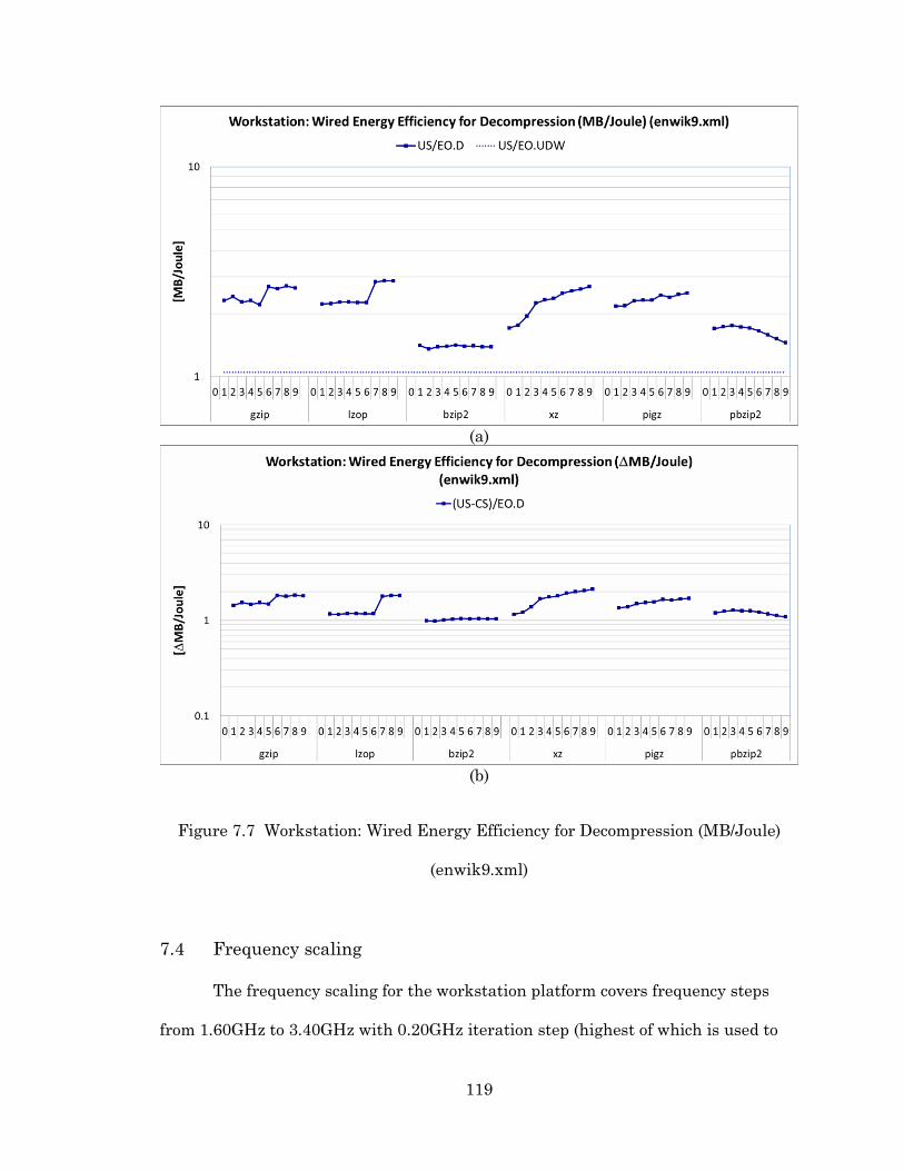
119

(a)

(b)

Figure 7.7 Workstation: Wired Energy Efficiency for Decompression (MB/Joule)

(enwik9.xml)

7.4 Frequency scaling

The frequency scaling for the workstation platform covers frequency steps

from 1.60GHz to 3.40GHz with 0.20GHz iteration step (highest of which is used to

120

describe and report results for Section 7.2 and Section 7.3). Similarly to Pandaboard,

a complete set of all tasks is repeated from those sections above for each frequency

step. Section 7.4.1 and Section 7.4.2 describe the effect of frequency scaling based on

throughput and energy efficiency metrics for the Local and Wired experiments.

7.4.1 Local


Figure 7.8 and Figure 7.9 show the compression and decompression through-

put on the Local experiment. The results confirm expectations that a higher clock

frequency means a higher compression and decompression throughput.

The highest compression throughput across all frequencies is achieved by

pigz -1, achieving 321.82 MB/sec on 3.40GHz and 151.37 MB/sec on 1.60GHz (Figure

7.8). Following pigz, lzop and pbzip2 come in second and third.

The highest decompression throughput across all frequencies is achieved by

lzop -7 to -9, achieving ~350 MB/sec on 3.40GHz and ~168 MB/sec on 1.60GHz

(Figure 7.9). Following lzop, pigz and pbzip2 come in second and third.

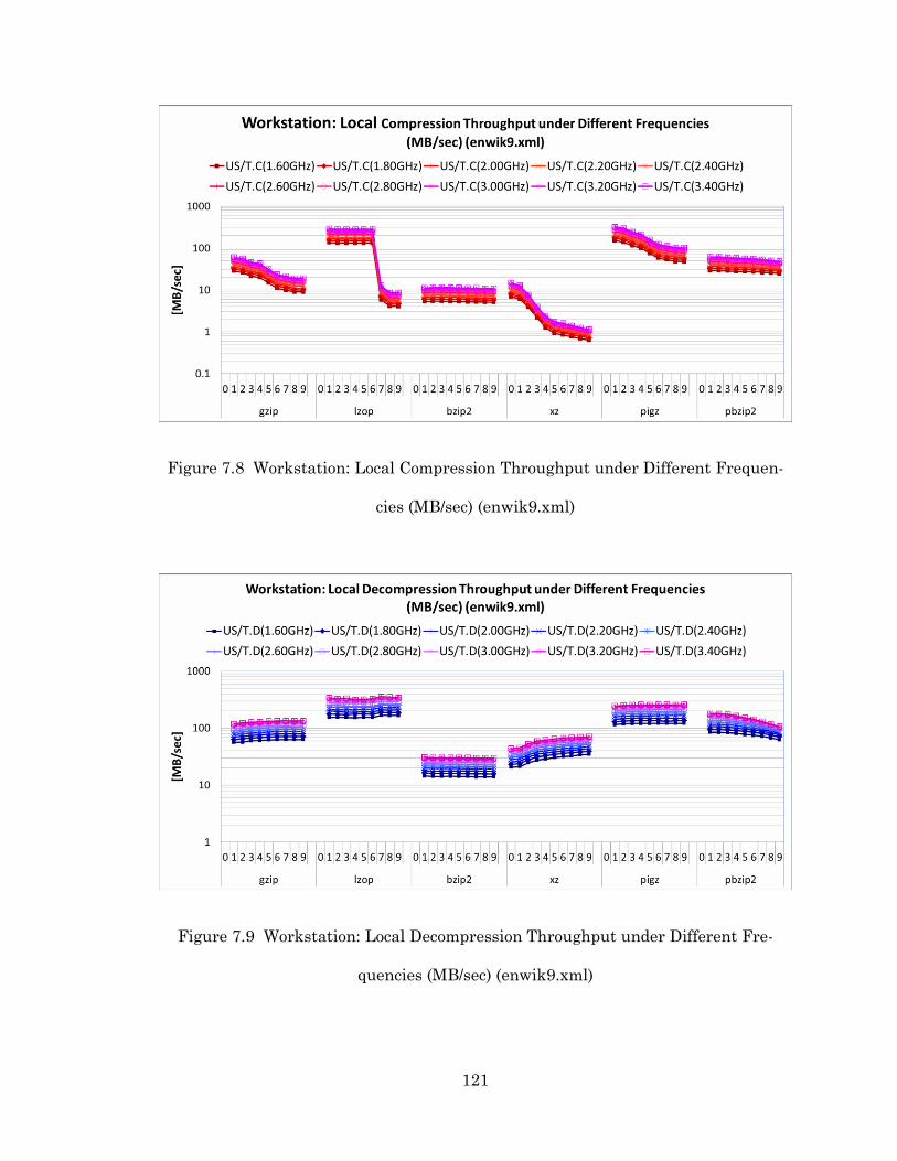
121

Figure 7.8 Workstation: Local Compression Throughput under Different Frequen-

cies (MB/sec) (enwik9.xml)

Figure 7.9 Workstation: Local Decompression Throughput under Different Fre-

quencies (MB/sec) (enwik9.xml)

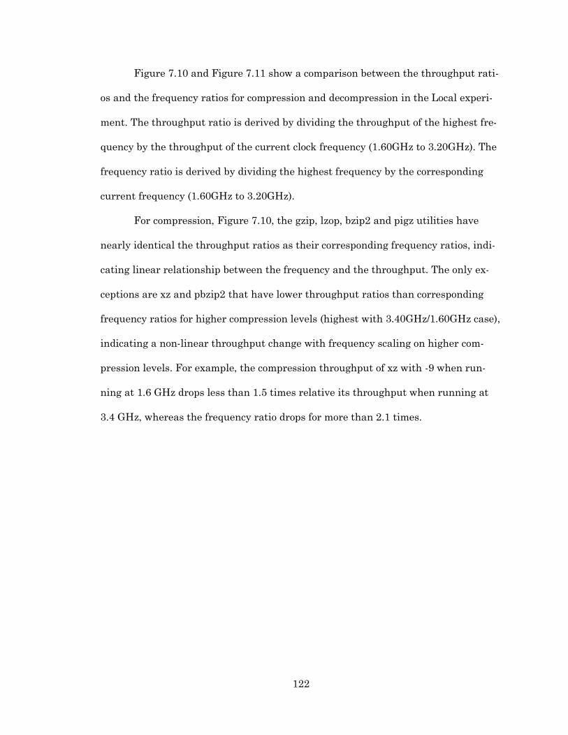
122

Figure 7.10 and Figure 7.11 show a comparison between the throughput rati-

os and the frequency ratios for compression and decompression in the Local experi-

ment. The throughput ratio is derived by dividing the throughput of the highest fre-

quency by the throughput of the current clock frequency (1.60GHz to 3.20GHz). The

frequency ratio is derived by dividing the highest frequency by the corresponding

current frequency (1.60GHz to 3.20GHz).

For compression, Figure 7.10, the gzip, lzop, bzip2 and pigz utilities have

nearly identical the throughput ratios as their corresponding frequency ratios, indi-

cating linear relationship between the frequency and the throughput. The only ex-

ceptions are xz and pbzip2 that have lower throughput ratios than corresponding

frequency ratios for higher compression levels (highest with 3.40GHz/1.60GHz case),

indicating a non-linear throughput change with frequency scaling on higher com-

pression levels. For example, the compression throughput of xz with -9 when run-

ning at 1.6 GHz drops less than 1.5 times relative its throughput when running at

3.4 GHz, whereas the frequency ratio drops for more than 2.1 times.

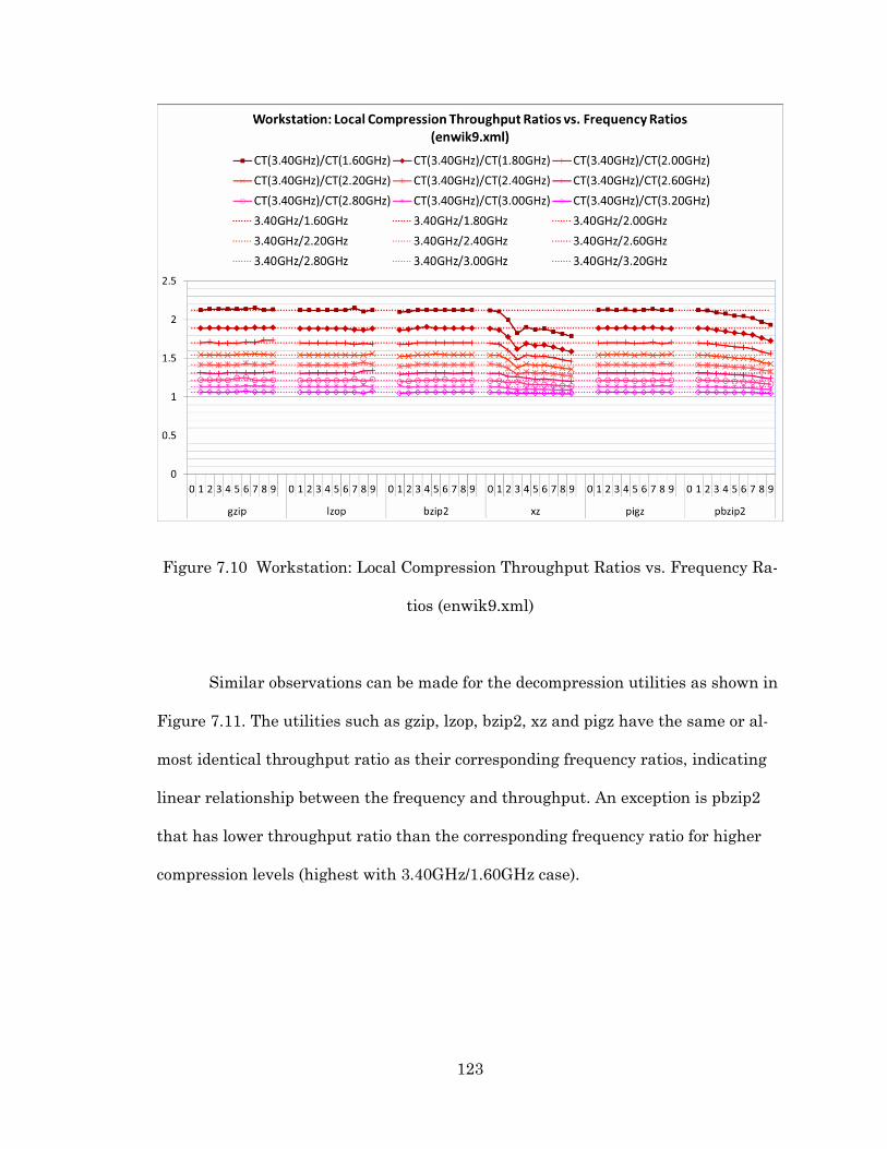
123

Figure 7.10 Workstation: Local Compression Throughput Ratios vs. Frequency Ra-

tios (enwik9.xml)

Similar observations can be made for the decompression utilities as shown in

Figure 7.11. The utilities such as gzip, lzop, bzip2, xz and pigz have the same or al-

most identical throughput ratio as their corresponding frequency ratios, indicating

linear relationship between the frequency and throughput. An exception is pbzip2

that has lower throughput ratio than the corresponding frequency ratio for higher

compression levels (highest with 3.40GHz/1.60GHz case).

124

Figure 7.11 Workstation: Local Decompression Throughput Ratios vs. Frequency

Ratios (enwik9.xml)



efficiency on the Local experiment.

The results shown in Figure 7.12 indicate that frequency scaling does not

provide significant changes in the energy efficiency of compression tasks for the ma-

jority of utilities. The highest energy efficiency is achieved by lzop -1 across all fre-

quencies, achieving ~17 MB/Joule.

125

Figure 7.12 Workstation: Local Energy Efficiency for Compression under Different

Frequencies (MB/Joule) (enwik9.xml)

The results shown in Figure 7.13 indicate that frequency scaling does not

provide significant change in the energy efficiency of decompression tasks for the

majority of utilities except for pigz and pbzip2. However, the highest energy efficien-

cy is achieved by lzop -1 across all frequencies, achieving ~20 MB/Joule.

126

Figure 7.13 Workstation: Local Energy Efficiency for Decompression under

Different Frequencies (MB/Joule) (enwik9.xml)

7.4.2 Wired



throughput in the Wired experiment while varying the processor clock frequency.

The highest compression throughput is achieved by pbzip2 with -9, 43.73

MB/sec at the highest clock frequency of 3.40GHz (Figure 7.14). The highest

throughput when processor is running at the lowest frequency of 1.6 GHz is

achieved by gzip -1, 27.70 MB/sec. The compression utilities that do not see a sub-

stantial change in the compression throughput with a change in frequency are lzop -

1 to -6 and pigz. The throughput of raw file upload benefits insignificantly with an

increase in the processor clock frequency.

127

Figure 7.14 Workstation: Wired Compression Throughput under Different

Frequencies (MB/sec) (enwik9.xml)

Figure 7.15 shows the decompression throughput while varying the processor

clock frequency. The results indicate that the majority of decompression utilities

(gzip, lzop, pigz, and pbzip2) do not see a substantial change in the throughput with

a change in the processor clock frequency. Notable exceptions are xz and bzip2 that

benefit from higher clock frequencies due to their high computational complexity.

The throughput of the uncompressed file transfer benefits insignificantly from an

increase in the clock frequency. The maximum decompression throughput is

achieved by xz -9, 51.93 MB/sec at 3.40GHz. The highest throughput at the lowest

frequency is achieved by pbzip2 -9, ~42 MB/sec at 1.60GHz.

128

Figure 7.15 Workstation: Wired Decompression Throughput under Different

Frequencies (MB/sec) (enwik9.xml)

Figure 7.16 and Figure 7.17 show the correlation between the throughput ra-

tios and the frequency ratios for the compression and decompression tasks in the

Wired experiment.

Unlike in the Local experiment, in the Wired experiment the throughput ra-

tio versus the frequency ratio distribution changes widely as illustrated in Figure

7.16. Now only bzip2 and to a certain extent xz exhibit scalable behavior – the

throughput ratios correspond to the frequency ratios. For the remaining utilities on-

ly highest compression levels show scalability. This can be explained as follows. The

compression throughput even with a low processor clock frequency is higher than

the achievable network throughput. This way, even if the processor is running at a

129

lower clock frequency, the network bandwidth is still going to be a limiting factor

rather than the computational time. bzip2 and xz with high computational complexi-

ty have the compression throughput that is below the achievable network through-

put, so they benefit from higher processor clock frequencies.

Figure 7.16 Workstation: Wired Compression Throughput Ratios vs. Frequencies

Ratios (enwik9.xml)

Similar observations can be made for the decompression tasks as shown in

Figure 7.17. For the majority of decompression tasks, the decompression throughput

is far greater than the network throughput during uncompressed file downloads, re-

gardless of the processor clock frequency. Consequently, by lowering the processor

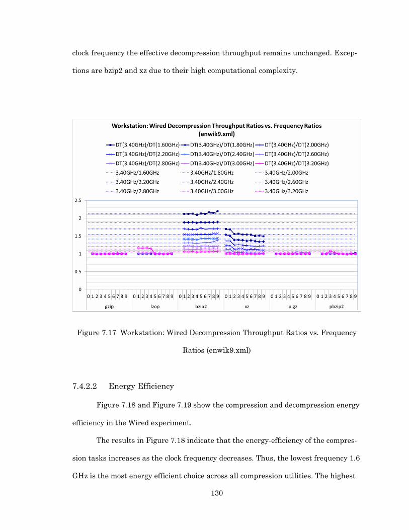
130

clock frequency the effective decompression throughput remains unchanged. Excep-

tions are bzip2 and xz due to their high computational complexity.

Figure 7.17 Workstation: Wired Decompression Throughput Ratios vs. Frequency

Ratios (enwik9.xml)



efficiency in the Wired experiment.

The results in Figure 7.18 indicate that the energy-efficiency of the compres-

sion tasks increases as the clock frequency decreases. Thus, the lowest frequency 1.6

GHz is the most energy efficient choice across all compression utilities. The highest

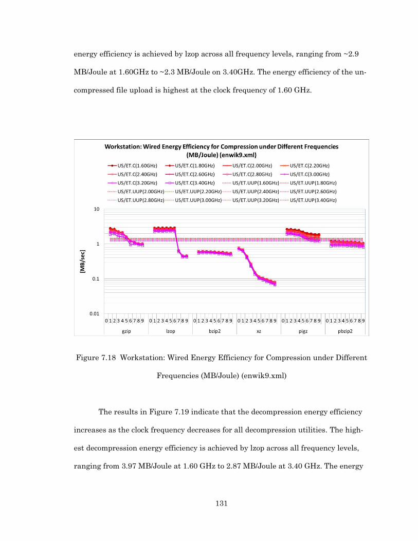
131

energy efficiency is achieved by lzop across all frequency levels, ranging from ~2.9

MB/Joule at 1.60GHz to ~2.3 MB/Joule on 3.40GHz. The energy efficiency of the un-

compressed file upload is highest at the clock frequency of 1.60 GHz.

Figure 7.18 Workstation: Wired Energy Efficiency for Compression under Different

Frequencies (MB/Joule) (enwik9.xml)

The results in Figure 7.19 indicate that the decompression energy efficiency

increases as the clock frequency decreases for all decompression utilities. The high-

est decompression energy efficiency is achieved by lzop across all frequency levels,

ranging from 3.97 MB/Joule at 1.60 GHz to 2.87 MB/Joule at 3.40 GHz. The energy

132

efficiency of the uncompressed file download also peaks for the lowest processor

clock frequency.

Figure 7.19 Workstation: Wired Energy Efficiency for Decompression under

Different Frequencies (MB/Joule) (enwik9.xml)

7.5 Conclusions

The experimental results for the workstation platform show that compression

tasks should utilize the lowest compression level to maximize throughput and ener-

gy efficiency, whereas decompression tasks should utilize the highest levels. A nota-

ble exceptions are bzip2 and pbzip2 where the computational complexity outweighs

the benefits of increased compression ratios.

133

Table 7.1 summarizes the compression and decompression throughput re-

sults. pigz and lzop perform the best for compression and decompression in the Local

experiment respectively. The best throughputs in the Wired experiment are

achieved by pbzip2 and xz for compression and decompression respectively.

Table 7.1 Throughputs on Workstation @ 3.40GHz


(UUP)

Decompression Raw

(UDW)

Best Utility

Th.C [MB/s]

Th.UUP [MB/s]

Best Utility

Th.D [MB/s]

Th.UDW [MB/s]

LOCAL pigz -1 321.82 lzop -7 358.97

WIRED pbzip2 -9 43.73 10.71 xz -9 51.93 10.72

Table 7.2 summarizes the compression and decompression energy efficiency.

The results indicate that compressed transfers could reduce the energy consumed

relative to the uncompressed transfers. lzop is the most energy-efficient for both the

Local and Wired experiment for compression and decompression. In the Wired ex-

periment, the most energy efficient compressed upload with lzop -1 achieves 2.3

MB/J, which ~1.84 times more energy-efficient than 1.25 MB/J achieved with the

uncompressed upload. The most energy-efficient decompressed download using lzop

with -9 achieves 2.86 MB/J, which is ~2.72 times better than the uncompressed

download that achieves 1.05 MB/J.

134

Table 7.2 Energy Efficiency on Workstation @ 3.40GHz


(UUP)

Decompression Raw

(UDW)

LOCAL

Best Utili-ty

EE.C [MB/J]

EE.UUP [MB/J]

Best Utility

EE.D [MB/J]

EE.UDW [MB/J]

Iidle = 0 A lzop -1 to -6 8.6 lzop -7 to -9 13.4

WIRED

Iidle = 0 A lzop -1 to -6 2.3 1.25 lzop -7 to -9 2.86 1.05

The use of parallel compression utilities such as pigz and pbzip2 offers gains

in the throughput and the energy efficiency for the compression and decompression

tasks relative to their sequential counterparts. Table 7.3 summarizes the through-

put and the energy efficiency gains of pigz and pbzip2 when compared to the sequen-

tial counterparts for all experimental cases.

Table 7.3 Performance Gains of Parallel Utilities on Workstation @ 3.40GHz


Local Wired

pigz ~80% 38.19%/3.67%

pbzip2 ~80% 77.98%/53.20%


Local Wired

pigz 0.00 0%/9.9% 0%/0%

0.25 32.86%/52.2% 13.91%/9.9%

0.50 48.38%/62.78% 22.06%/9.20%

0.75 56.64%/67.65% 25.56%/8.6%

pbzip2 0.00 0%/0% 0%/0%

0.25 27.5%/34.49% 37.5%/28.7%

0.50 43.5%/50.99% 58.13%/37.4%

0.75 54.05%/58.82% 64.51%/41.26%

135

The frequency scaling analysis indicates that the compression and decom-

pression throughputs suffer from lower frequency, which can be explained easily by

the general observation that the execution time of each utility goes up with lowering

of frequency. The energy efficiency increases when the clock frequency goes down for

the selected utilities in the Local (factor of ~1.1 for pigz and pbzip2) and the Wired

experiment (by factor of ~1.4 for all except pbzip2).

136

CHAPTER 8

CONCLUSIONS

This thesis describes an experimental evaluation of recent implementations

of common compression utilities on three selected platforms, Pandaboard, a state-of-

the-art mobile development platform, Raspberry Pi, a low-end mobile computer plat-

form, and a workstation computer platform. The evaluation includes measurements

of compression and decompression times and the total and overhead energies con-

sumed by compression and decompression tasks. Metrics, such as compression ratio,

compression/decompression throughput, and compression/decompression energy effi-

ciency, are reported for all compression levels and platforms. Based on the results of

this thesis, practical guidelines for selecting the most energy-efficient utilities are

provided depending on the usage scenario. Across all systems and experiments, a

single utility that always performs above network transfer for both throughput and

energy efficiency is lzop. The lzop utility outperforms network transfer even on

Raspberry Pi were all other compression utilities fail. Additionally, lzop outperforms

network transfer for both throughput and energy efficiency when considering all Iidle

currents for both Pandaboard and Raspberry Pi. Even that utilities such as pigz,

gzip or xz outperform lzop, specifically for decompression on the slowest network

throughput (on the Wireless experiment), they often fail to outperform network

transfer in either throughput or energy efficiency in selected cases. Thus, if there is

a need for one uniform utility that can perform well for both throughput and energy

efficiency across different platforms and different network speeds, lzop provides this

137

by demonstrating that it can work well and never fail any of the experiments con-

ducted across all evaluation hardware platforms of diverse hardware complexity and

performance. Additional observations, from all experiments conducted in this thesis,

indicate that it is always better to use the lowest compression level for compression

tasks and the highest compression level for decompression tasks. Performing de-

compression is also always more energy efficient for both mobile platforms and the

workstation platform. When comparing performance of three evaluation platforms,

Pandaboard provides higher energy efficiency over Raspberry Pi and the work-

station for the Local, Wired and Wireless experiments.

Several general observations are made across three systems:

The lzop utility is the only utility which outperforms network transfer

across all systems and all experiments for both throughput and energy ef-

ficiency.

The utilities such as xz, pigz and gzip, while exceeding lzop on selected

network experiments (the decompression in particular), often fail to out-

perform network throughput for compression or energy efficiency (either

in another experiment or on another platform).

For throughput and energy efficiency, it is always best to select the lowest

compression level for compression and the highest compression level for

decompression.

The gain of using parallel utilities instead of sequential counterparts in

networked experiments is limited by the compression ratio and the net-

work upload and download throughputs, i.e., CR*T.UUP and CR*T.UDW.

Scaling frequency down always reduces throughput.

138

Scaling frequency down, when Iidle of 0 A, always produces higher energy

efficiency.

Scaling frequency down, when Iidle of 0.25 A or greater, always produces

lower energy efficiency.

The findings can be used to direct energy optimizations of data transfers in

mobile and workstation applications by encouraging development of data transfer

frameworks that are conscientious of the mobile device’s energy status. For example,

a server could easily store multiple copies of the same file, compressed with different

utilities and compression levels, to allow the mobile device to choose, based on its

capabilities, currently available network bandwidth, energy status, and user prefer-

ences, which version of a file to download. Compression utility, such as lzop, can be

integrated as a basic compression and decompression choice for software reposito-

ries, so that devices downloading files can automatically download the compressed

file and decompress them on their systems. However, if proper condition such as

slow network speed, is met, mobile device can instead download file compressed us-

ing the xz utility. Additionally, mobile devices, could decide which frequency level to

use during download or upload of files.

139

REFERENCES

[1] “Smart phones overtake client PCs in 2011 | Canalys.” [Online]. Available:

http://www.canalys.com/newsroom/smart-phones-overtake-client-pcs-2011. [Ac-

cessed: 01-Jun-2012].

[2] “Global Smartphone Shipments Hit a Record 700 Million Units in 2012.”

[Online]. Available:

http://www.strategyanalytics.com/default.aspx?mod=reportabstractviewer&a0=

8142. [Accessed: 28-Jan-2013].

[3] “PC Volume to Grow Almost 5% in 2012, But Will Expand Further in 2013 and

Beyond, According to IDC - prUS23549112.” [Online]. Available:

http://www.idc.com/getdoc.jsp?containerId=prUS23549112#.UQbvHme0cil. [Ac-

cessed: 28-Jan-2013].

[4] “Cisco Visual Networking Index: Global Mobile Data Traffic Forecast Update,

2011–2016 [Visual Networking Index (VNI)] - Cisco Systems.” [Online]. Avail-

able:

http://www.cisco.com/en/US/solutions/collateral/ns341/ns525/ns537/ns705/ns827

/white_paper_c11-520862.html. [Accessed: 01-Jun-2012].

[5] D. Huffman, “A Method for the Construction of Minimum-Redundancy Codes,”

Proceedings of the IRE, vol. 40, no. 9, pp. 1098–1101, Sep. 1952.

[6] J. Rissanen and G. G. Langdon, “Arithmetic Coding,” IBM Journal of Research

and Development, vol. 23, no. 2, pp. 149–162, Mar. 1979.

[7] J. Ziv and A. Lempel, “A universal algorithm for sequential data compression,”

IEEE Transaction on Information Theory, vol. 23, no. 3, pp. 337–343, 1977.

140

[8] M. Burrows and D. J. Wheeler, “A Block-sorting Lossless Data Compression

Algorithm,” Digital SRC, 1994.

[9] “Mobile Wireless LAN - WiLinkTM 6.0 Solutions.” [Online]. Available:

http://www.ti.com/general/docs/wtbu/wtbuproductcontent.tsp?templateId=6123

&navigationId=12762&contentId=29993&INTC=SensorTag&HQS=sensortag-

pr-lp5. [Accessed: 08-Feb-2013].

[10] K. Barr and K. Asanović, “Energy aware lossless data compression,” in Pro-

ceedings of the 1st International Conference on Mobile Systems, Applications

and Services (MobiSys’03), 2003, pp. 231–244.

[11] K. C. Barr and K. Asanović, “Energy-aware lossless data compression,” ACM

Transactions on Computer Systems, vol. 24, no. 3, pp. 250–291, Aug. 2006.

[12] R. Xu, Z. Li, C. Wang, and P. Ni, “Impact of data compression on energy con-

sumption of wireless-networked handheld devices,” in Distributed Computing

Systems, 2003. Proceedings. 23rd International Conference on, 2003, pp. 302 –

311.

[13] R. Kothiyal, V. Tarasov, P. Sehgal, and E. Zadok, “Energy and performance

evaluation of lossless file data compression on server systems,” in Proceedings

of SYSTOR 2009: The Israeli Experimental Systems Conference, New York, NY,

USA, 2009, pp. 4:1–4:12.

[14] “The gzip home page.” [Online]. Available: http://www.gzip.org/. [Accessed: 25-

May-2012].

[15] M. Oberhumer, “lzop file compressor (oberhumer.com OpenSource).” [Online].

Available: http://www.lzop.org/. [Accessed: 25-May-2012].

141

[16] “bzip2 : Home.” [Online]. Available: http://www.bzip.org/. [Accessed: 25-May-

2012].

[17] “XZ Utils.” [Online]. Available: http://tukaani.org/xz/. [Accessed: 25-May-2012].

[18] I. Pavlov, “7-Zip.” [Online]. Available: http://www.7-zip.org/. [Accessed: 25-

May-2012].

[19] “pigz - Parallel gzip.” [Online]. Available: http://zlib.net/pigz/. [Accessed: 25-

May-2012].

[20] J. Gilchrist, “Parallel BZIP2 (PBZIP2).” [Online]. Available:

http://compression.ca/pbzip2/. [Accessed: 25-May-2012].

[21] E. Rotem, A. Naveh, A. Ananthakrishnan, E. Weissmann, and D. Rajwan,

“Power-Management Architecture of the Intel Microarchitecture Code-Named

Sandy Bridge,” IEEE Micro, vol. 32, no. 2, pp. 20–27, Mar. 2012.

[22] “Pandaboard.” [Online]. Available: http://pandaboard.org/. [Accessed: 28-May-

2012].

[23] “OMAPTM 4 Platform - OMAP4430/OMAP4460.” [Online]. Available:

http://www.ti.com/omap4430. [Accessed: 02-Jun-2012].

[24] “Linaro: open source software for ARM SoCs.” [Online]. Available:

http://www.linaro.org/. [Accessed: 28-May-2012].

[25] “Raspberry Pi | An ARM GNU/Linux box for $25. Take a byte!” [Online]. Avail-

able: http://www.raspberrypi.org/. [Accessed: 17-Jan-2013].

[26] “FrontPage - Raspbian.” [Online]. Available: http://www.raspbian.org/. [Ac-


[27] “Arch Linux ARM | Arch Linux ARM.” [Online]. Available:

http://archlinuxarm.org/. [Accessed: 17-Jan-2013].

142

[28] “Raspbmc.” [Online]. Available: http://www.raspbmc.com/. [Accessed: 17-Jan-

2013].

[29] “OpenELEC - The living room PC for everyone.” [Online]. Available:

http://openelec.tv/. [Accessed: 17-Jan-2013].

[30] “Android | Raspberry Pi.” [Online]. Available:

http://www.raspberrypi.org/archives/tag/android. [Accessed: 17-Jan-2013].

[31] “Android and Apple iOS Capture a Record 92 Percent Share of Global

Smartphone Shipments in Q4 2012.” [Online]. Available:

http://www.strategyanalytics.com/default.aspx?mod=reportabstractviewer&a0=

8155. [Accessed: 28-Jan-2013].

[32] “Tizen | An open source, standards-based software platform for multiple device

categories.” [Online]. Available: https://www.tizen.org/. [Accessed: 17-Jan-2013].

[33] “MeeGo.” [Online]. Available: https://meego.com/. [Accessed: 17-Jan-2013].

[34] “Open webOS.” [Online]. Available: http://www.openwebosproject.org/. [Ac-


[35] “Mozilla — Firefox OS — mozilla.org.” [Online]. Available:

http://www.mozilla.org/en-US/firefoxos/. [Accessed: 17-Jan-2013].

[36] “Ubuntu for phones | Ubuntu.” [Online]. Available:

http://www.ubuntu.com/devices/phone. [Accessed: 17-Jan-2013].

[37] “Ubuntu for Android | Devices | Ubuntu.” [Online]. Available:

http://www.ubuntu.com/devices/android. [Accessed: 17-Jan-2013].

[38] “Usage Statistics and Market Share of Operating Systems for Websites, Janu-

ary 2013.” [Online]. Available:

http://w3techs.com/technologies/overview/operating_system/all/. [Accessed: 17-

Jan-2013].

143

[39] “Certified hardware | Ubuntu.” [Online]. Available:

http://www.ubuntu.com/certification/. [Accessed: 17-Jan-2013].

[40] “Ubuntu TV | Devices | Ubuntu.” [Online]. Available:

http://www.ubuntu.com/devices/tv. [Accessed: 17-Jan-2013].

[41] “STEAMWORKS - The Big Picture.” [Online]. Available:

http://www.steampowered.com/steamworks/thebigpicture.php. [Accessed: 17-

Jan-2013].

[42] “Linux | Valve.” [Online]. Available: http://blogs.valvesoftware.com/linux/. [Ac-


[43] “IEEE Xplore - Cloud Computing for Mobile Users: Can Offloading Computa-

tion Save Energy?” [Online]. Available:

http://ieeexplore.ieee.org/xpls/abs_all.jsp?arnumber=5445167. [Accessed: 02-

Nov-2012].

[44] N. K. Nithi and A. J. de Lind van Wijngaarden, “Smart power management for

mobile handsets,” Bell Lab. Tech. J., vol. 15, no. 4, pp. 149–168, Mar. 2011.

[45] A. Pathak, Y. C. Hu, and M. Zhang, “Where is the energy spent inside my app?:

fine grained energy accounting on smartphones with Eprof,” in Proceedings of

the 7th ACM european conference on Computer Systems, New York, NY, USA,

2012, pp. 29–42.

[46] A. Pathak, Y. C. Hu, M. Zhang, P. Bahl, and Y.-M. Wang, “Fine-grained power

modeling for smartphones using system call tracing,” in Proceedings of the sixth

conference on Computer systems, New York, NY, USA, 2011, pp. 153–168.

[47] T. Li and L. K. John, “Run-time modeling and estimation of operating system

power consumption,” SIGMETRICS Perform. Eval. Rev., vol. 31, no. 1, pp. 160–

171, Jun. 2003.

144

[48] A. Carroll and G. Heiser, “An analysis of power consumption in a smartphone,”

in Proceedings of the 2010 USENIX conference on USENIX annual technical

conference, Berkeley, CA, USA, 2010, pp. 21–21.

[49] W. L. Bircher and L. K. John, “Complete System Power Estimation Using Pro-

cessor Performance Events,” IEEE Transactions on Computers, vol. 61, no. 4,

pp. 563 –577, Apr. 2012.

[50] H. David, E. Gorbatov, U. R. Hanebutte, R. Khanna, and C. Le, “RAPL:

Memory power estimation and capping,” in 2010 ACM/IEEE International

Symposium on Low-Power Electronics and Design (ISLPED), 2010, pp. 189 –

194.

[51] J. Treibig, G. Hager, and G. Wellein, “LIKWID: A Lightweight Performance-

Oriented Tool Suite for x86 Multicore Environments,” in 2010 39th Interna-

tional Conference on Parallel Processing Workshops (ICPPW), 2010, pp. 207 –

216.

[52] G. H. Jan Treibig, “LIKWID: Lightweight Performance Tools,” 2011.

[53] “Large Text Compression Benchmark.” [Online]. Available:

http://cs.fit.edu/~mmahoney/compression/text.html. [Accessed: 17-Jan-2013].

[54] “50’000€ Prize for Compressing Human Knowledge.” [Online]. Available:

http://prize.hutter1.net/. [Accessed: 17-Jan-2013].

[55] “Human Knowledge Compression Contest: Detailed Rules for Participation.”

[Online]. Available: http://prize.hutter1.net/hrules.htm. [Accessed: 17-Jan-

2013].

[56] “LikwidPowermeter - likwid - likwid-powermeter: Tool for accessing RAPL

counters and query Turbo mode steps on Intel processor - Lightweight perfor-

mance tools - Google Project Hosting.” [Online]. Available:

145

http://code.google.com/p/likwid/wiki/LikwidPowermeter. [Accessed: 17-Jan-

2013].

performance and energy efficiency ... - electrical & computermilenka/docs/armend.thesis.pdf ·...

Documents